Extended isochron rays in prestack depth (map) migration
A.A. Duchkov∗ and M.V. de Hoop∗
∗Purdue University,
150 N.University st.,
West Lafayette, IN, 47907
e-mail: [email protected]
(December 15, 2008)
Extended isochron rays
Running head: Extended isochron rays
ABSTRACT
Many processes in seismic data analysis and imaging can be identified with solution op-
erators of evolution equations. These include data downward continuation and velocity
continuation, where continuation relates to the evolution parameter in such equations. In
this paper, we address the question whether isochrons defined by imaging operators can be
identified with wavefronts of solutions to an evolution equation. To this end, we consider
the double-square-root equation and the space on which its solutions are defined. We refer
to this space as the “prestack imaging volume”, which has coordinates (sub)surface mid-
point, offset, (two-way) time and depth. By manipulating the double-square-root operator,
we obtain an evolution equation in two-way time describing prestack depth map migration
generating extended (pre-stack) images. The propagation of singularities by its solutions is
described by extended isochron rays, the corresponding wavefronts of which are extended
isochrons. Conventional isochrons are obtained in such a construction by restriction to
1

zero subsurface offset. The evolution equation implies a Hamiltonian that generates the
extended isochron rays in phase space.
2
INTRODUCTION
Many processes in seismic data analysis and imaging can be identified with solution op-
erators (propagators) of evolution equations. These include data downward continuation
(Clayton (1978); Claerbout (1985); Biondi (2006a)) and velocity continuation (Fomel (1994);
Goldin (1994); Hubral et al. (1996); Adler (2002)), where continuation relates to the evolu-
tion parameter in such equations. (For a comprehensive theory and framework, see Duchkov
et al. (2008); Duchkov and De Hoop (2008).) In this paper, we address the question whether
isochrons derived from imaging operators can be identified with wavefronts of solutions to
an evolution equation.
The role of continuation in imaging, viewed as a mapping of data to an image, is not
so obvious. Zero-offset (ZO) depth migration, based on the exploding reflector concept,
has been formulated in terms of wave propagation using half-velocities (Lowenthal et al.
(1976)) assuming the absence of caustics, while ZO time migration has been formulated in
terms of velocity continuation (Fomel, 1994). The geometry of prestack depth migration
can be understood in terms of isochrons describing how a surface data sample (viewed as a
point source) smears in the subsurface while contributing to an image. Iversen (2004, 2005)
studied how these isochrons can be connected via so-called isochron rays. Here, through
the introduction of extended isochron rays, we derive a Hamiltonian generating these rays
and an associated evolution equation describing prestack depth migration.
It is interesting to note that Iversen (2004) proposed different “rays” connecting isochrons,
namely, with what he calls source, receiver and combined parametrizations. We show that
it is only the combined parametrization that leads to rays generated by a Hamiltonian.
Even when the Hamiltonian is not known one can still determine whether a set of curves
3

can be generated by one, namely, by checking an integrability condition. This was done,
in the constant background velocity case, for the different parametrizations in Duchkov
et al. (2008). Isochron rays were revisited by Silva and Sava (2008) with the purpose to
implement a map migration procedure generating common-offset gathers in heterogeneous
background velocity models. However, their choice of “rays” does not admit a Hamilto-
nian (and associated phase and group velocities) to be constructed. Our Hamiltonian for
extended isochron rays implies a method based on a single system of ray tracing equations
for prestack depth map migration generating an extended image.
Our derivations and constructions make use of a 2n-dimensional “prestack imaging vol-
ume” with coordinates (sub)surface midpoint, offset, (two-way) time and depth (for 3-D
seismics, n = 3). This volume appears naturally in the downward-continuation approach
to imaging, but is also fundamental in our general geometrical analysis. We consider the
double square-root (DSR) equation, an evolution equation in depth. We rewrite the DSR
equation in the form of an evolution equation in two-way time. The fronts associated with
the solutions to this equation are extended isochrones. Prestack depth (map) migration
is then formulated as an initial value problem with the data generating a source in the
evolution equation. We can view this fomulation as an extension of the exploding reflec-
tor concept from ZO to prestack data using a single evolution equation. An alternative
extension, using two wave operators, was proposed by Biondi (2006b).
DATA CONTINUATION IN DEPTH: SUMMARY
In this section, we summarize data continuation in depth and formulate modelling and
imaging, subject to the single scattering approximation, in terms of solving Cauchy initial
value problems in depth. The basic operator appearing in these processes is the so-called
4

double-square-root (DSR) operator, PDSR = PDSR(z,xs,xr,Ds,Dr, Dt) (Belonosova and
Alekseev (1967); Clayton (1978); Claerbout (1985)). Here, Dt corresponds in the Fourier
domain with multiplication by frequency, ω, Dr corresponds in the Fourier domain with
multiplication by wavevector, kr, and Ds corresponds in the Fourier domain with multipli-
cation by wavevector, ks.
The DSR operator can be viewed as a pseudodifferential operator. Its principal symbol,
denoted here by a subscript 1, determines the associated propagation of singularities and
ray geometry, that is, the kinematics. To guarantee dynamically correct propagation, one
also needs the so-called subprincipal part of the symbol (De Hoop (1996); ?); ?); Stolk
and De Hoop (2005)). We suppress this contribution in the presentation here, the focus
being on the geometry. The principal symbol of the DSR operator is given by the standard
expression,
PDSR1 (z,xs,xr,ks,kr, ω) = ω
√1
c(z,xs)2− ‖ks‖2
ω2+ ω
√1
c(z,xr)2− ‖kr‖2
ω2, (1)
while considering ω > 0; z ∈ [0, Z] denotes depth, where Z denotes the maximum depth
considered.
Modelling: Upward continuation
Seismic reflection data can be modelled – in the Born approximation – with an inhomoge-
neous DSR equation (Stolk and De Hoop (2005), suppressing the (de)composition operators
in the flux normalization):
(−)[∂z − iPDSR(z,xs,xr,Ds,Dr, Dt)]u = δ(t)E(z,xs,xr), u|z=Z = 0, (2)
where
E(z,xs,xr) = δ(xr − xs)12(c−3δc)
(z, 1
2(xr + xs)); (3)
5
δc(z,x) is the function containing the rapid velocity variations representative of the scat-
terers, superimposed on a smooth background model described by the function c(z,x).
Equation (2) is solved in the direction of decreasing z (upward, and forward in time).
The data are then modelled by the solution of (2) restricted to z = 0: u(z = 0,xs,xr, t).
The corresponding solution operator is schematically illustrated in Fig. 1 (b). In general,
we denote the propagator associated with the left-hand side of (2), from depth z to depth
z, by H(z,z). Throughout, we assume that the DSR condition holds: For all source-receiver
combinations present in the acquisition geometry the source rays (each connecting a scat-
tering or image point to a source) and receiver rays (each connecting a scattering or image
point to a receiver) become nowhere horizontal, see Fig. 1 (a). We note that the DSR con-
dition can be generalized to hold with respect to a curvilinear coordinate system defining a
“pseudodepth” Stolk et al. (2008).
DSR rays
The propagation of singularities by solutions of (2) is governed by the Hamiltonian,
HDSR(z,xs,xr, kz,ks,kr, ω) = −(kz − PDSR1 (z,xs,xr,ks,kr, ω)), (4)
cf. (1). We denote the DSR rays by
X = (xs(z, .),xr(z, .), t(z, .)), K = (ks(z, .),kr(z, .), ω(z, .)), (5)
which solve the Hamilton system
d(xs,xr, t)dz
=∂HDSR
∂(ks,kr, ω),
d(ks,kr, ω)dz
= − ∂HDSR
∂(xs,xr, t).
Here, depth is the evolution parameter. Slowness vectors are obtained from the wavevectors
through k/ω. In Fig. 2 (a) we show the typical representation of the geometry as a couple
6
of rays in two copies of physical space, viz. one with coordinates (z,xs) and one with
coordinates (z,xr). In Fig. 2 (b) we show a DSR ray as a single curve defined by (5) in
the extended volume with coordinates (xs,xr, z, t), which we will refer to as the “prestack
imaging volume”.
A DSR ray considered as a curve in the “prestack imaging volume” (see Fig. 2 (b))
satisfies the DSR condition if it does not turn in the z or in the t direction. Thus t(z, .) in
(5) is a monotonous function in z. This in turn implies that each DSR ray intersects planes
z = const and t = const at most once. Thus any of these planes can be chosen to pose an
initial value problem for data continuation, and either z or t can be used as an evolution
parameter.
Imaging: Downward continuation
Imaging reflection data, d = d(xs,xr, t), can be formulated as solving the initial value
problem,
[∂z − iPDSR(z,xs,xr,Ds,Dr, Dt)]u = 0, u(0,xs,xr, t) = d(xs,xr, t), (6)
now to be solved in the direction of increasing z (downward, and backward in time). The
image at (z,x) is obtained upon subjecting the solution of (6) to the imaging conditions:
u(z,x,x, t = 0). We have that u(z, ., ., .) = H∗(0,z)d, where ∗ denotes taking the adjoint.
Through the above formulation, imaging is described to act in the “prestack imaging
volume” as a composition of a continuation operator (in depth) and restriction operators
(imaging conditions).
7
DATA CONTINUATION IN TWO-WAY TRAVELTIME
Here, we discuss an alternative form of data continuation, namely in two-way traveltime
rather than depth. To begin with, let, for given (z,xs,xr,ks,kr), Θ denote the mapping
ω → kz = PDSR1 (z,xs,xr,ks,kr, ω)
(cf. (4)). Under the DSR condition there exists an inverse mapping,
Θ−1 : kz → ω = Θ−1(z,xs,xr, kz,ks,kr),
that solves the equation (Stolk and De Hoop, 2005, Lemma 4.1):
kz = PDSR1 (z,xs,xr,ks,kr,Θ−1(z,xs,xr, kz,ks,kr)). (7)
The inverse mapping also defines the principal symbol, P TWT1 , of a pseudodifferential op-
erator:
P TWT1 (xs,xr, z,ks,kr, kz) = Θ−1(z,xs,xr, kz,ks,kr)
=crcs
|c2−|
kz
√c2+ + k−2
z (‖kr‖2 − ‖ks‖2) c2− − 2
√c2sc
2r + k−2
z (‖kr‖2c2r − ‖ks‖2c2
s) c2−, (8)
where cr = c(z,xr), cs = c(z,xs), c2− = c(z,xs)2 − c(z,xr)2 and c2
+ = c(z,xs)2 + c(z,xr)2.
We note that formula (8) admits the limit c2− → 0 to be taken.
Remark. It appears often useful to transform coordinates from subsurface lateral source
and receiver coordinates to subsurface midpoint and offset coordinates,
xr = x + h, xs = x− h, ks = 12(kx − kh), kr = 1
2(kx + kh). (9)
This coordinate transform can be applied to the symbol of the DSR operator (Shubin, 2001,
Thm. 4.2); we get
PDSR1 (z,x,h,kx,kh, ω) = PDSR
1 (z,xs(x,h),xr(x,h),ks(kx,kh),kr(kx,kh), ω). (10)
8
Then
P TWT1 (z,x,h, kz,kx,kh)
=crcs
|c2−|
kz
√√√√c2+ +
〈kx,kh〉k2
z
c2− −
√4c2
sc2r −
(‖kx‖2 + ‖kh‖2)k2
z
(c2−)2 + 2
〈kx,kh〉k2
z
c2+c2
−, (11)
where, now, cs = c(z,x− h) and cr = c(z,x + h).
Modelling: Forward continuation
We now consider the initial value problem,
[∂t − iP TWT1 (xs,xr, z,Ds,Dr, Dz)]u = 0, u(z,xs,xr, 0) = E(z,xs,xr) (12)
(cf. (3)) to be solved in the direction of increasing two-way time t (thus decreasing z). We
note that the solution at z = 0 (to leading asymptotic order) models the reflection data, that
is, u(0,xs,xr, t) = u(0,xs,xr, t). Equation (12) generalizes the notion of exploding reflector
modelling zero-offset reflection data to exploding extended reflector modelling pre-stack
reflection data.
DSR rays revisited
The propagation of singularities by solutions of (12) is governed by the Hamiltonian,
HTWT (z,xs,xr, ω, kz,ks,kr) = ω − P TWT1 (z,xs,xr, kz,ks,kr)). (13)
Now, we denote the DSR rays by
X = (z(t, .),xs(t, .),xr(t, .)), K = (kz(t, .),ks(t, .),kr(t, .)), (14)
which solve the Hamilton system
d(z,xs,xr)dt
=∂HTWT
∂(kz,ks,kr),
d(kz,ks,kr)dt
= − ∂HTWT
∂(z,xs,xr).
9
Here, two-way time is the evolution parameter.
Remark (c(z) models). In the case of a vertically inhomogeneous velocity model, we have
c(z,xr) = c(z,xs) = c(z). We could use the expressions above, but it is more straightforward
to rederive the Hamiltonian directly from (4) and (1), in xs, xr coordinates, that is,
HTWT (z,xs,xr, ω, kz,ks,kr)
= ±(
ω − kzc(z)2
√k−4
z (‖ks‖2 − ‖kr‖2)2 + 2k−2z (‖kr‖2 + ‖ks‖2) + 1
). (15)
Transforming the Hamiltonian from subsurface lateral source and receiver coordinates to
subsurface midpoint and offset coordinates, yields
HTWT (z,x,h, ω, kz,kx,kh) = ω − kzc(z)2
√k−4
z 〈kx,kh〉2 + k−2z (‖kx‖2 + ‖kh‖2) + 1. (16)
We note that for constant background velocity, c(z) = v say, equation (15) reduces to
(Sava, 2003, (3)); equation (16) reduces to the Fourier domain counterpart of (Fomel, 2003,
(A-10)).
Imaging: Backward continuation
Imaging reflection data, d = d(xs,xr, t), can be formulated as solving the initial value
problem,
(−)[∂t − iP TWT1 (xs,xr, z,Ds,Dr, Dz)]u = δ(z)d(xs,xr, t), u|t=T = 0, (17)
to be solved in the direction of decreasing two-way time t (thus increasing z). The extended
image at (z,xs,xr) is obtained upon subjecting the solution to the imaging condition:
u(z,xs,xr, t = 0). We have that u(., ., ., 0) =∫ T0 H∗
(t′,0)d(., ., t′) dt′ if H(t,t) is the propagator,
10
from time t to time t, associated with the left-hand side of (12). Continuation in two-way
time is schematically illustrated in Fig. 3.
Remark (exploding reflectors). We use the Hamiltonians for data continuation in
two-way traveltime and depth to revisit the exploding reflector model used in the early
development of seismic imaging. For a vertically inhomogeneous velocity model, c(z), the
Hamiltonian HTWT in (16) does not depend on h, and thus the phase variable kh remains
constant in the course of downward continuation (dkhdt = −∂HTWT
∂h = 0). For zero source-
receiver offset (ZO) surface data, kh = 0 (this follows immediately from the symmetry of
common midpoint gathers) and it remains zero for all t. Then equation (16) reduces to
the Hamiltonian for zero-offset data modelling in the “exploding reflector” approach by
Lowenthal et al. (1976); Claerbout (1985); Cheng and Coen (1984):
ω − kzc(z)2
√1 + ‖kx‖2k−2
z = HZO(x, z, ω,kx, kz), (18)
where we recognize the “half-velocity” 12c(z) typical for the “exploding reflector” model.
We note that we describe, here, the “exploding reflector” model by a first-order evolution
equation instead of a second -order wave equation.
EXTENDED ISOCHRON RAYS
Isochrons form the “impulse response” of an imaging operator, that is, they are the fronts
in extended image space with coordinates, here, (z,x,h), that originate from a particular
data sample.
We first consider the ray-geometrical impulse response associated with equation (17),
which may be constructed by shooting a fan of rays originating at a “point source”. Us-
ing the Hamiltonian in (16), we generate the backward flow (equivalent to (14) but time
11
reversed)
X(t) = (z(t, .),x(t, .),h(t, .)), K(t) = (kz(t, .),kx(t, .),kh(t, .)), (19)
supplemented with the “initial” conditions:
(z(t0, .),x(t0, .),h(t0, .)) = X0 = (0,x0,h0),
(kz(t0, .),kx(t0, .),kh(t0, .)) = K0 = (kz0, kx0, kh0).
While letting K0 vary in all possible directions, we connect the endpoints, X(t = 0),
to form an extended isochron corresponding with two-way time t0, see Fig. 4 (a) where
(z0, x0, h0) = (0, 0, .5) (two-dimensional seismics) and t0 = 1, 3, 5. By increasing t0 we trace
extended isochron rays, see the thin black lines in Fig. 4 (b). Essentially, we have obtained
a Hamilton flow description of map migration.
We note that HTWT is anisotropic even though the underlying wave equation has been
taken in an isotropic medium. The isochron ray tangent vectors define the group velocity
being normal to the slowness surface defined by HTWT = 0.
Restriction: Conventional isochron rays
Conventional isochrons are defined in image space with coordinates (z,x). Functions defined
on the image space are obtained from functions defined on the “prestack imaging volume” by
restricting h to zero. This is the way how isochrons are obtained from extended isochrons.
The restriction is illustrated in Fig. 4 (b): The fat grey curves are conventional isochrons
(t0 = 1, 3, 5) while the fat black line is a conventional isochron ray. We note that extended
isochrons exist for every (positive) t0, while they will not intersect the h = 0 plane for t0
less then the direct-wave traveltime from source to receiver. Indeed, conventional isochrons
12

do not exist for t0 < 1 in the model example shown in Fig. 4 (b). We note that this fact
causes some complications with initializing conventional isochron rays, see Iversen (2004).
Extended isochron rays are solutions to Hamilton equations as described in (19). We
now establish the connection between extended isochron rays and conventional isochron
rays (in image space) for common (source-receiver) offset migration as defined in Iversen
(2004). For simplicity, we will discuss the case of two-dimenional seismics when x and
h are one-dimensional. As was mentioned earlier, the direction of an extended isochron
ray is determined by the wavevector K0 = (kz0, kx0, kh0). The components of this vector
are subject to the constraint that HTWT = 0. We then fix kx0, which constraint can be
imposed under the “common offset” restriction. With these two constraints, we have only
one degree of freedom left for the three components of K0. The resulting one-parameter
family of extended isochron rays, for a constant velocity case, is shown in Fig. 4 (b) by
thin lines. This family of rays intersects the image space at h = 0 along a smooth curve,
illustrated in Fig. 4 (b) by a fat line. This smooth curve is a conventional isochron ray.
It is not at all immediate, however, that the curve obtained by connecting the intersec-
tion points of extended isochron rays form a ray again. First, we need to to check whether
this curve can be parameterized by two-way time, t0 (the natural evolution parameter for
isochron rays). Second, we need to check that varying kx0 provides us with an integrable
family of curves. We have carried out these checks for the constant velocity case (Duchkov
et al. (2008)) shown in Fig. 4 (b). Indeed, in this case the fat line constructed as described
above coincides with a conventional isochron ray in the “combined parametrization” as in-
troduced by Iversen (2004). On the other hand, we argue that the “rays” as proposed in
Silva and Sava (2008) are not related to solutions to any Hamilton system and hence should
not be called rays.
13
Extended isochron rays in the presence of caustics
We consider a velocity model with a low-velocity lens imbedded in homogeneous medium:
c(x, z) = 1− .4 e−9(x2+(1−z)2). (20)
This model generates caustics in the propagating wavefield but still satisfies the DSR condi-
tion: The low velocity lens is not strong enough to produce turning rays for comparatively
short offsets. Conventional (common-offset) isochrons were constructed for this medium
in (Stolk, 2002, Fig. 5, bottom). Isochron shown in that figure corresponds to initial pa-
rameters (t0, x0, h0, z0) = (4.73, 0, .2, 0) and has a rather complicated form. The extended
isochron surface for these initial data is shown in Fig. 5 (a) and a few extended isochron
rays are shown by thin lines in Fig. 5 (b).
Besides the fact that extended isochrons have now complicated forms, the way we con-
struct conventional isochrons and isochron rays remains the same. A conventional isochron
is an intersection of the extended isochron surface in Fig. 5 (a) with an image plane corre-
sponding to h = 0. This intersection is shown as grey curve in Fig. 5 (b). A better view of
this curve is shown in Fig. 6 labelled as t0 = 4.72. Another two conventional isochrons are
shown with grey curves as well for t0 = 2 and t0 = 3.8. One can see that for small two-way
times conventional isochron is a connected curve (t0 = 2). Then a second piece appear
around t0 = 3.8 and for two-way time t0 = 4.72 one can see 9 smooth branches making up
two piece-wise disjoint figures.
For obtaining a conventional isochron ray (Iversen, 2004, combined parametrization)
we shoot a one-parameter family of extended isochron rays corresponding to a fixed kx0 as
shown in Fig. 5 (b) by thin black lines, for kx0 = .2. The thick black line corresponds to a
14
conventional isochron ray: it is an intersection of a fan of extended isochron rays with h = 0
plane. A more complicated case of a conventional isochron ray, corresponding to kx0 = .02,
is shown in Fig. 6. We observe that it consists of two disjoint branches (thick black lines)
that can appear when extended isochron rays intersect the plane h = 0 more than once.
Second branch of the conventional isochron ray appears around t0 = 3.8 when conventional
isocnron splits onto two pieces.
CONCLUSION
We have introduced the notion of extended isochron rays. These rays are defined in a
“prestack imaging volume” with coordinates (sub)surface midpoint, offset, (two-way) time
and depth, and are generated by a Hamiltonian. Our construction of this Hamiltonian
depends on the DSR condition, which can be generally formulated in terms of curvilinear
(sub)surface coordinates (Stolk et al. (2008)). Extended isochrons appear as wavefronts
associated with solutions to an evolution equation. We establish how conventional isochrons
are obtained from extended isochrons through a restriction to zero subsurface offset.
The initialization of extended isochron rays appears as natural as the initialization of rays
in geometrical acoustics, unlike the initialization of conventional isochron rays as described
in (Iversen, 2004, 2005). In these papers, also, no Hamiltonian was obtained. Indeed, we
argue that, through data continuation in (pseudo)depth or two-way time, the “prestack
imaging volume” appears natural in the (geometrical) analysis of imaging operators.
The results presented in this paper imply a formulation of prestack map depth migration
via the extended image in terms of a Hamiltonian flow. Such a formulation is amenable to
a “curvelet” decomposition of the corresponding imaging operator (Douma and De Hoop
15
(2007); de Hoop et al. (2008)).
ACKNOWLEDGMENTS
The authors would like to thank the members, BP, ConocoPhillips, ExxonMobil, Statoil-
Hydro, and Total, of the Geo-Mathematical Imaging Group for financial support.
16
REFERENCES
Adler, F., 2002, Kirchhoff image propagation: Geophysics, 67, 126–134.
Belonosova, A. and A. Alekseev, 1967, About one formulation of the inverse kinematic
problem of seismics for a two-dimensional continuously heterogeneous medium: Some
methods and algorithms for interpretation of geophysical data (in Russian), 137–154,
Nauka.
Biondi, B., 2006a, 3D seismic imaging, volume 14: Investigations in Geophysics Series,
SEG.
——–, 2006b, Prestack exploding-reflectors modeling for migration velocity analysis: Ex-
panded Abstracts, SEG, 25 (1), 3056.
Cheng, G. and S. Coen, 1984, The relationship between Born inversion and migration of
common-midpoint stacked data: Geophysics, 49, 2117–2131.
Claerbout, J., 1985, Imaging the earth’s interior: Blackwell Scientific Publishing.
Clayton, R., 1978, Common midpoint migration: Technical Report, Stanford University,
SEP-14.
De Hoop, M., 1996, Generalization of the Bremmer coupling series: J. Math. Phys., 37,
3246–3282.
de Hoop, M., H. Smith, G. Uhlmann, and R. van der Hilst, 2008, Seismic imaging with
the generalized radon transform: A curvelet transform perspective: Inverse Problems, in
print.
Douma, H. and M. De Hoop, 2007, Leading-order seismic imaging using curvelets: Geo-
physics, 72, S231–S248.
Duchkov, A. and M. De Hoop, 2008, Velocity continuation in the downward continuation
approach to seismic imaging: J. Geoph. Int., in print.
17
Duchkov, A., M. De Hoop, and A. Sa Barreto, 2008, Evolution-equation approach to seismic
image, and data, continuation: Wave Motion, 45, 952–969.
Fomel, S., 1994, Method of velocity continuation in the problem of seismic time migration:
Russian Geology and Geophysics, 35, No. 5, 100–111.
——–, 2003, Velocity continuation and the anatomy of residual prestack time migration:
Geophysics, 68, 1650–1661.
Goldin, S., 1994, Superposition and continuation of operators used in seismic imaging:
Russian Geology and Geophysics, No. 9, 131–145.
Hubral, P., M. Tygel, and J. Schleicher, 1996, Seismic image waves: Geophys. J. Int., 125,
431–442.
Iversen, E., 2004, The isochron ray in seismic modeling and imaging: Geophysics, 69,
1053–1070.
——–, 2005, Tangent vectors of isochron rays and velocity rays expressed in global cartesian
coordinates: Stud. Geophys. Geod., 49, 525–540.
Lowenthal, D., L. Lu, R. Roberson, and J. Sherwood, 1976, The wave equation applied to
migration: Geophysical Prospecting, 24, 380–399.
Sava, P., 2003, Prestack residual migration in the frequency domain: Geophysics, 68, 634–
640.
Shubin, M. A., 2001, Pseudodifferential operators and spectral theory: Springer.
Silva, E. and P. Sava, 2008, Modeling and imaging with isochron rays: Technical Report,
Colorado School of Mines, CWP-602, 193–204.
Stolk, C., 2002, Microlocal analysis of the scattering angle transform: Communications in
Partial Differential Equations, 27 (9-10), 1879–1900.
Stolk, C. and M. De Hoop, 2005, Modeling of seismic data in the downward continuation
18

approach: SIAM J. Appl. Math., 65, 1388–1406.
Stolk, C., M. De Hoop, and W. Symes, 2008, Kinematics of shot-geophone migration:
Geophysics, submitted.
19

LIST OF FIGURES
1 Upward/downward data continuation. (a) Upward/downward data continuation as
solutions to initial value problems (2), (6) with the homogeneous DSR equation; (b) DSR
modelling operator that solves initial problem (2) with the inhomogeneous DSR equation.
2 Geometry of the DSR operator for up/downward data continuation. (a) DSR ray
viewed as a pair of conventional rays; (b) DSR ray viewed as solution to the DSR Hamilton
equations (cf. (5)) with X defining position on a ray and K defining its orientation.
3 Forward/backward two-way time continuation for modelling and imaging. (a) Mod-
elling as a solution of initial problem (12); (b) imaging as a solution of initial problem (17).
4 Notion of (extended) isochrons. (a) Extended isochrons for two-way traveltimes
t0 = 1, 3, 5; (b) Conventional isochrons (thick grey lines) and isochron rays (thick black
lines) in the image space obtained from extended isochrons and rays by restricting h to
zero.
5 Extended isochrons and rays in case of caustics. (a) Extended isochron for two-way
traveltime t0 = 4.72; (b) Conventional isochron (thick grey line) and isochron ray (thick
black line) in the image space corresponding to slice h = 0; corresponding extended isochron
rays are shown by thin black lines.
6 Conventional (common-offset) isochrons and an isochron ray in the presence of
caustics. Grey lines - conventional isocrons as intersection of extended isochron surfaces
with h = 0 plane. They correspond to two-way time t0 = 2, 3.8 and 4.7 seconds (from top
to bottom); note that the lowest one is identical to the one in (Stolk (2002),Fig. 5, bottom).
Thick black lines - conventional isochron ray as intersection of a fan of extended isochron
rays (for fixed kx0 = .02) with h = 0 plane.
20
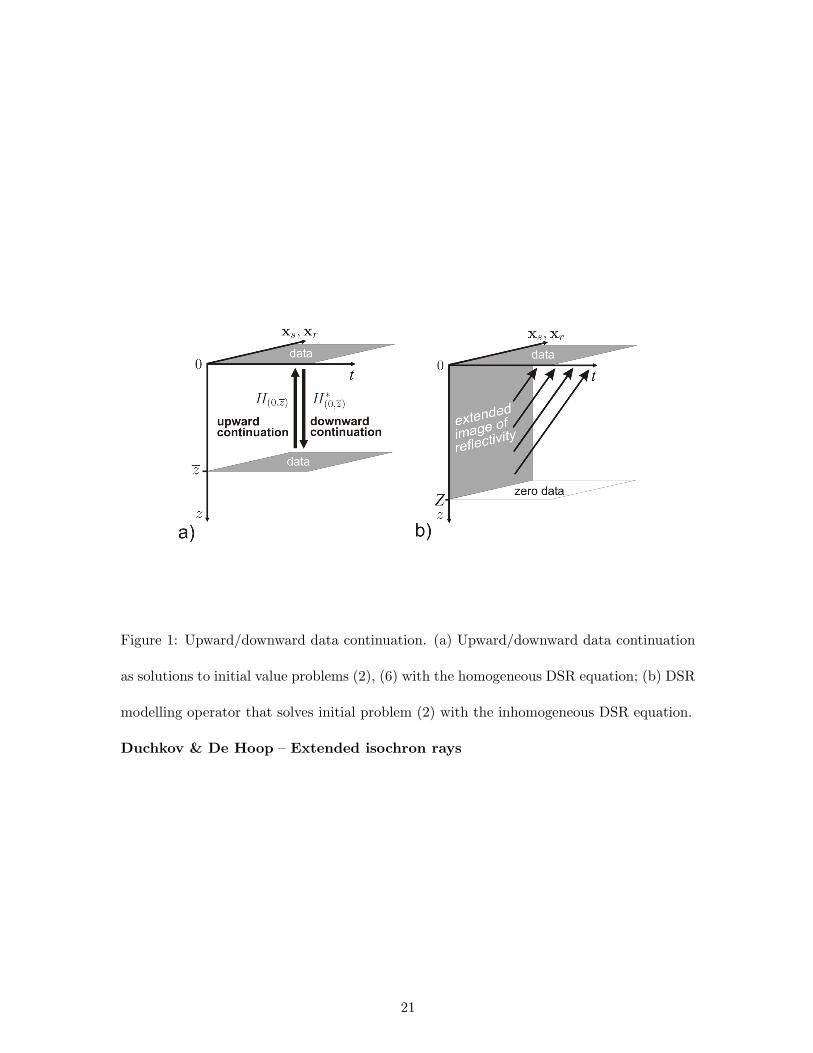
Figure 1: Upward/downward data continuation. (a) Upward/downward data continuation
as solutions to initial value problems (2), (6) with the homogeneous DSR equation; (b) DSR
modelling operator that solves initial problem (2) with the inhomogeneous DSR equation.
Duchkov & De Hoop – Extended isochron rays
21
Figure 2: Geometry of the DSR operator for up/downward data continuation. (a) DSR ray
viewed as a pair of conventional rays; (b) DSR ray viewed as solution to the DSR Hamilton
equations (cf. (5)) with X defining position on a ray and K defining its orientation.
Duchkov & De Hoop – Extended isochron rays
22
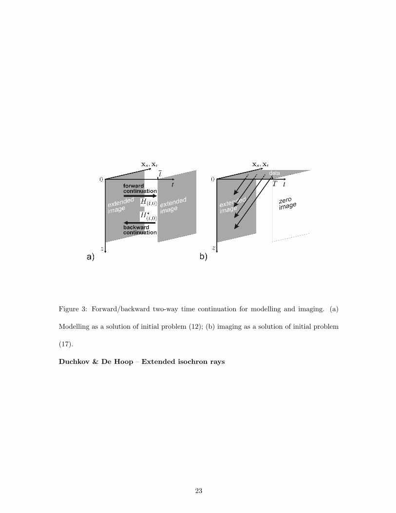
Figure 3: Forward/backward two-way time continuation for modelling and imaging. (a)
Modelling as a solution of initial problem (12); (b) imaging as a solution of initial problem
(17).
Duchkov & De Hoop – Extended isochron rays
23
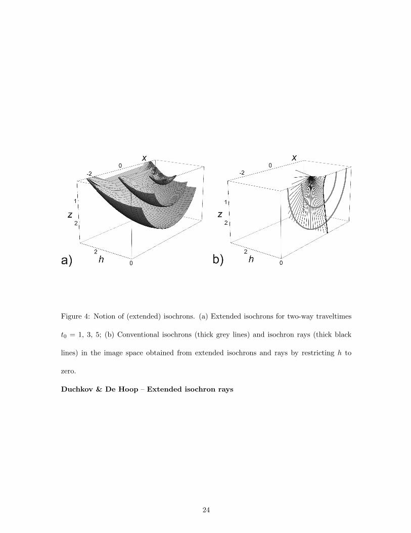
Figure 4: Notion of (extended) isochrons. (a) Extended isochrons for two-way traveltimes
t0 = 1, 3, 5; (b) Conventional isochrons (thick grey lines) and isochron rays (thick black
lines) in the image space obtained from extended isochrons and rays by restricting h to
zero.
Duchkov & De Hoop – Extended isochron rays
24

Figure 5: Extended isochrons and rays in case of caustics. (a) Extended isochron for two-
way traveltime t0 = 4.72; (b) Conventional isochron (thick grey line) and isochron ray (thick
black line) in the image space corresponding to slice h = 0; corresponding extended isochron
rays are shown by thin black lines.
Duchkov & De Hoop – Extended isochron rays
25
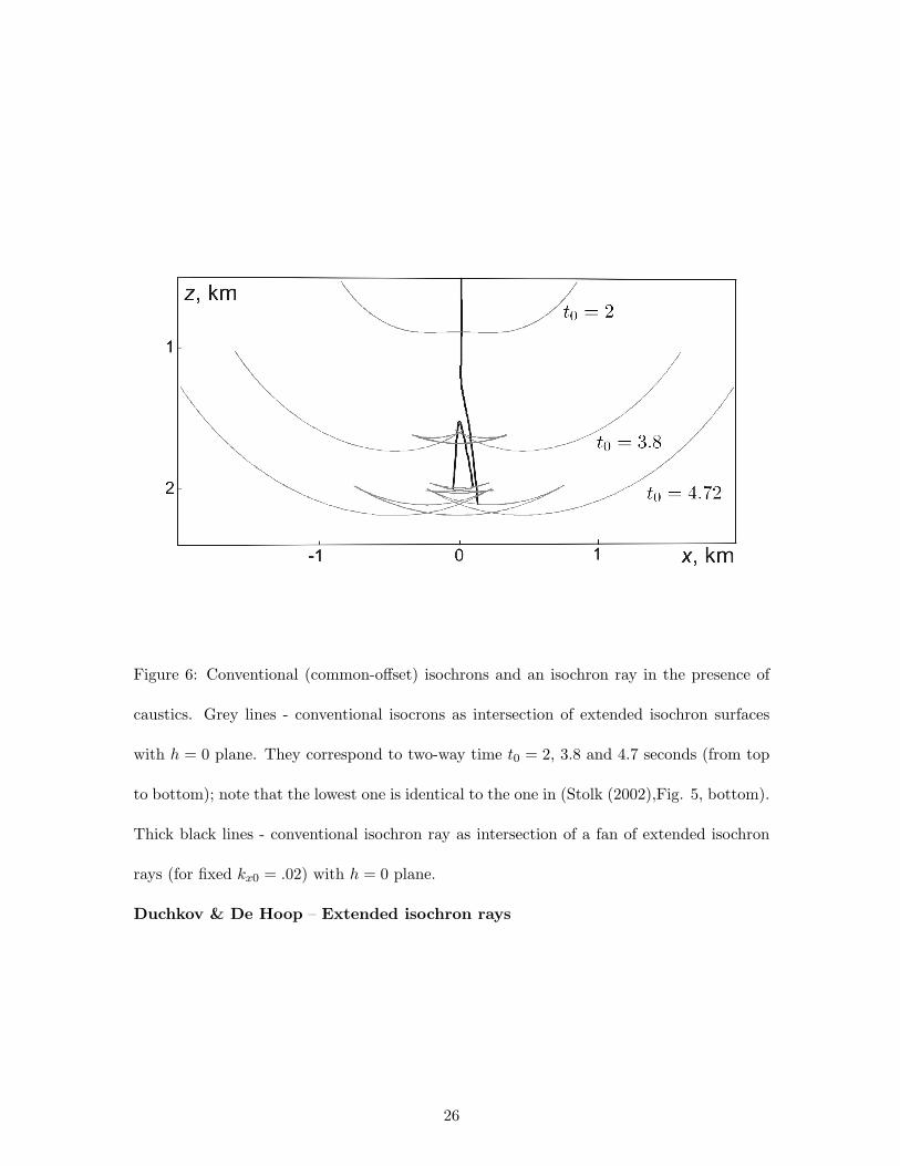
Figure 6: Conventional (common-offset) isochrons and an isochron ray in the presence of
caustics. Grey lines - conventional isocrons as intersection of extended isochron surfaces
with h = 0 plane. They correspond to two-way time t0 = 2, 3.8 and 4.7 seconds (from top
to bottom); note that the lowest one is identical to the one in (Stolk (2002),Fig. 5, bottom).
Thick black lines - conventional isochron ray as intersection of a fan of extended isochron
rays (for fixed kx0 = .02) with h = 0 plane.
Duchkov & De Hoop – Extended isochron rays
26


