Estimation of spectra
• Fourier Transform• Periodogram• Spectral leakage & resolution & bias• Tapered Periodogram• Welch‘s method• Confidence Intervals
Further reading on spectral analysis:Bendat & Piersol: Random data, Wiley 2000Percival & Walden: Spectral analysis for physical applications, Cambridge 1993
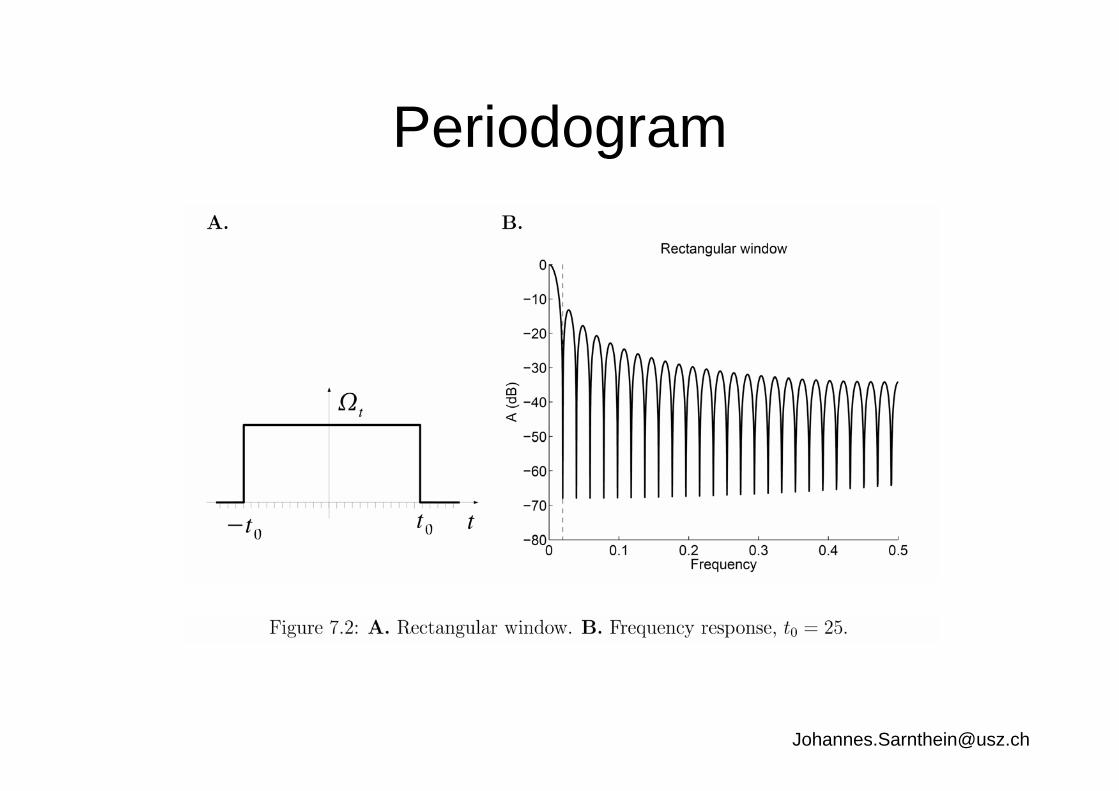
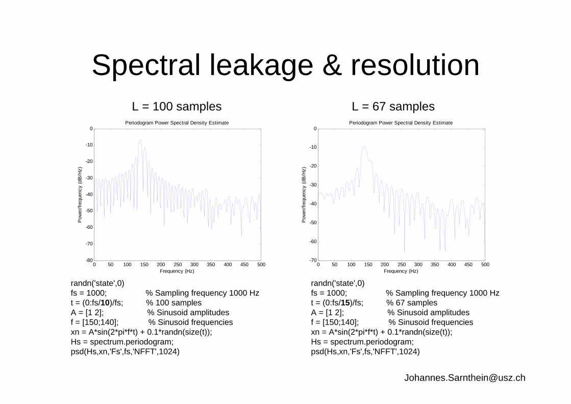
Spectral leakage & resolution
randn('state',0)fs = 1000; % Sampling frequency 1000 Hzt = (0:fs/10)/fs; % 100 samplesA = [1 2]; % Sinusoid amplitudesf = [150;140]; % Sinusoid frequenciesxn = A*sin(2*pi*f*t) + 0.1*randn(size(t));Hs = spectrum.periodogram;psd(Hs,xn,'Fs',fs,'NFFT',1024)
randn('state',0)fs = 1000; % Sampling frequency 1000 Hzt = (0:fs/15)/fs; % 67 samplesA = [1 2]; % Sinusoid amplitudesf = [150;140]; % Sinusoid frequenciesxn = A*sin(2*pi*f*t) + 0.1*randn(size(t));Hs = spectrum.periodogram;psd(Hs,xn,'Fs',fs,'NFFT',1024)
L = 100 samples L = 67 samples
0 50 100 150 200 250 300 350 400 450 500-70
-60
-50
-40
-30
-20
-10
0
Frequency (Hz)
Pow
er/fr
eque
ncy
(dB
/Hz)
Periodogram Power Spectral Density Estimate
0 50 100 150 200 250 300 350 400 450 500-80
-70
-60
-50
-40
-30
-20
-10
0
Frequency (Hz)
Pow
er/fr
eque
ncy
(dB
/Hz)
Periodogram Power Spectral Density Estimate
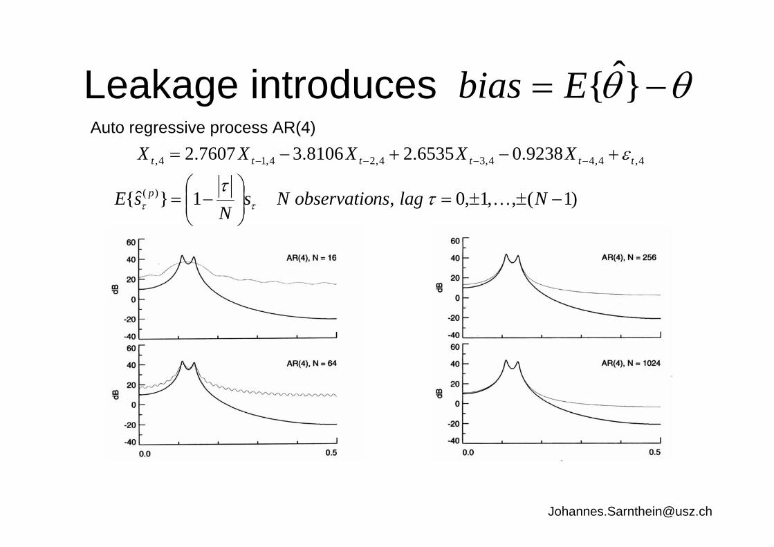
Leakage introducesAuto regressive process AR(4)
θθ −= }ˆ{Ebias
4,4,44,34,24,14, 9238.06535.28106.37607.2 tttttt XXXXX ε+−+−= −−−−
)1(,,1,0,1}ˆ{ )( −±±=⎟⎟⎠
⎞⎜⎜⎝
⎛−= NlagnsobservatioNs
NsE p Kτ
τττ
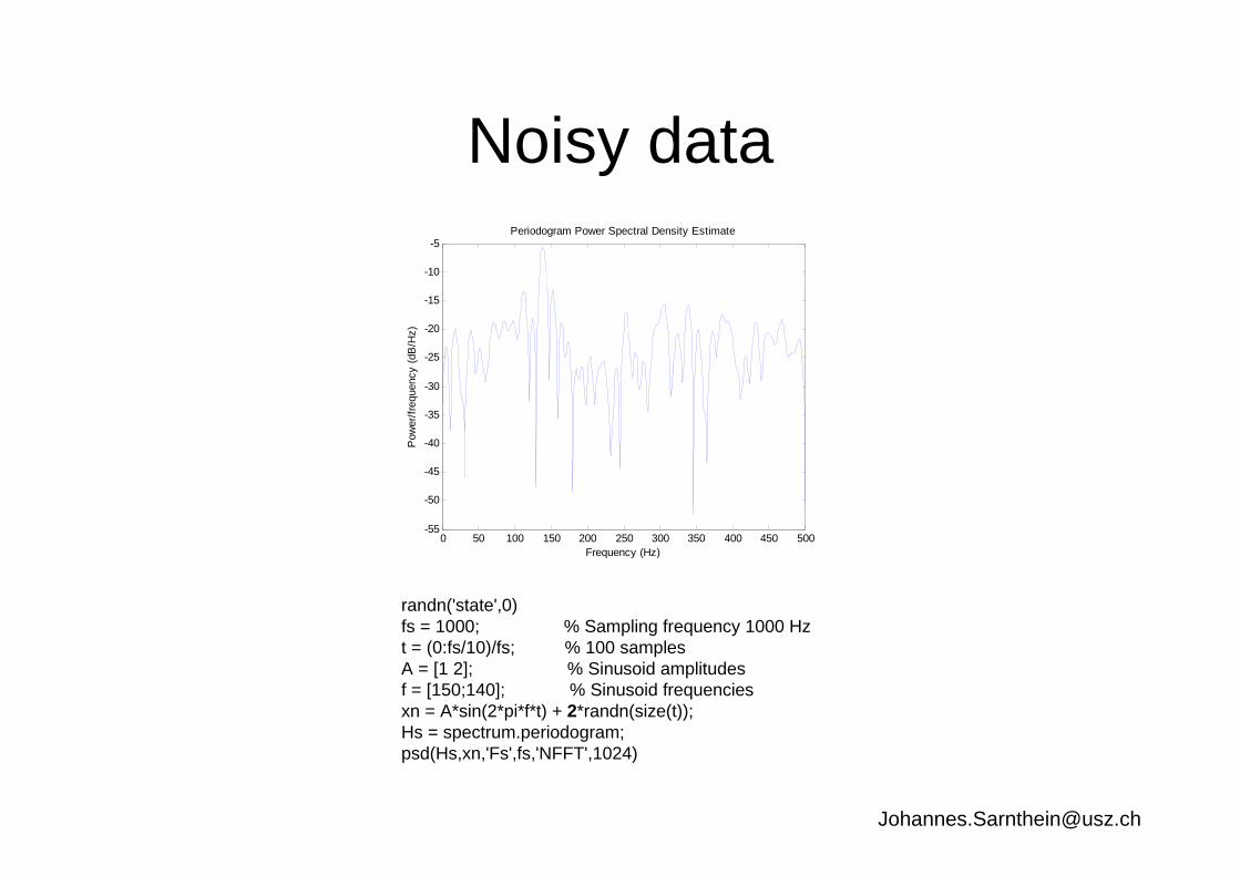
Noisy data
randn('state',0)fs = 1000; % Sampling frequency 1000 Hzt = (0:fs/10)/fs; % 100 samplesA = [1 2]; % Sinusoid amplitudesf = [150;140]; % Sinusoid frequenciesxn = A*sin(2*pi*f*t) + 2*randn(size(t));Hs = spectrum.periodogram;psd(Hs,xn,'Fs',fs,'NFFT',1024)
0 50 100 150 200 250 300 350 400 450 500-55
-50
-45
-40
-35
-30
-25
-20
-15
-10
-5
Frequency (Hz)
Pow
er/fr
eque
ncy
(dB
/Hz)
Periodogram Power Spectral Density Estimate
Tapered Periodogram I
10 20 30 40 500
0.2
0.4
0.6
0.8
1
Samples
Ampl
itude
Time domain
0 0.2 0.4 0.6 0.8-150
-100
-50
0
50
Normalized Frequency (×π rad/sample)
Mag
nitu
de (d
B)
Frequency domain
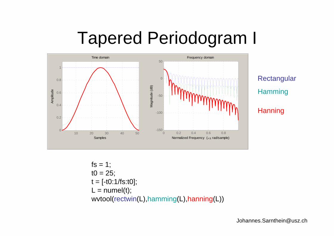
Rectangular
Hamming
Hanning
fs = 1;t0 = 25;t = [-t0:1/fs:t0];L = numel(t);wvtool(rectwin(L),hamming(L),hanning(L))
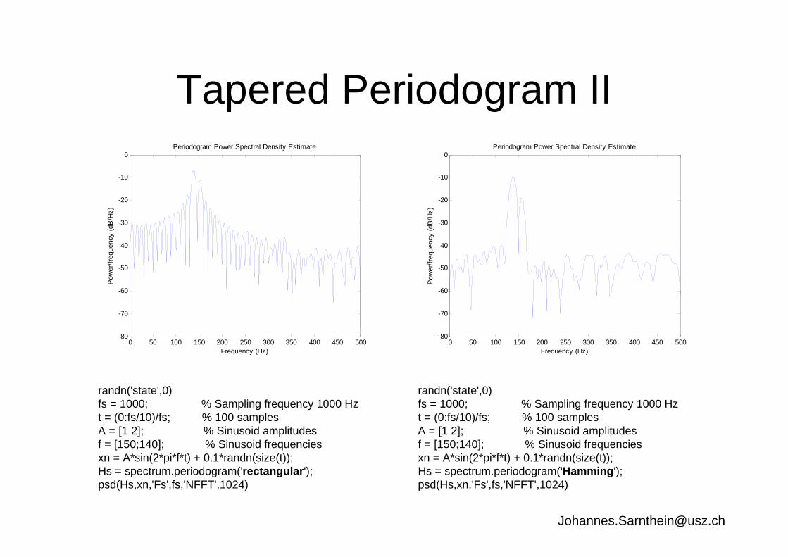
Tapered Periodogram II
randn('state',0)fs = 1000; % Sampling frequency 1000 Hzt = (0:fs/10)/fs; % 100 samplesA = [1 2]; % Sinusoid amplitudesf = [150;140]; % Sinusoid frequenciesxn = A*sin(2*pi*f*t) + 0.1*randn(size(t));Hs = spectrum.periodogram('rectangular');psd(Hs,xn,'Fs',fs,'NFFT',1024)
randn('state',0)fs = 1000; % Sampling frequency 1000 Hzt = (0:fs/10)/fs; % 100 samplesA = [1 2]; % Sinusoid amplitudesf = [150;140]; % Sinusoid frequenciesxn = A*sin(2*pi*f*t) + 0.1*randn(size(t));Hs = spectrum.periodogram('Hamming');psd(Hs,xn,'Fs',fs,'NFFT',1024)
0 50 100 150 200 250 300 350 400 450 500-80
-70
-60
-50
-40
-30
-20
-10
0
Frequency (Hz)
Pow
er/fr
eque
ncy
(dB
/Hz)
Periodogram Power Spectral Density Estimate
0 50 100 150 200 250 300 350 400 450 500-80
-70
-60
-50
-40
-30
-20
-10
0
Frequency (Hz)
Pow
er/fr
eque
ncy
(dB
/Hz)
Periodogram Power Spectral Density Estimate
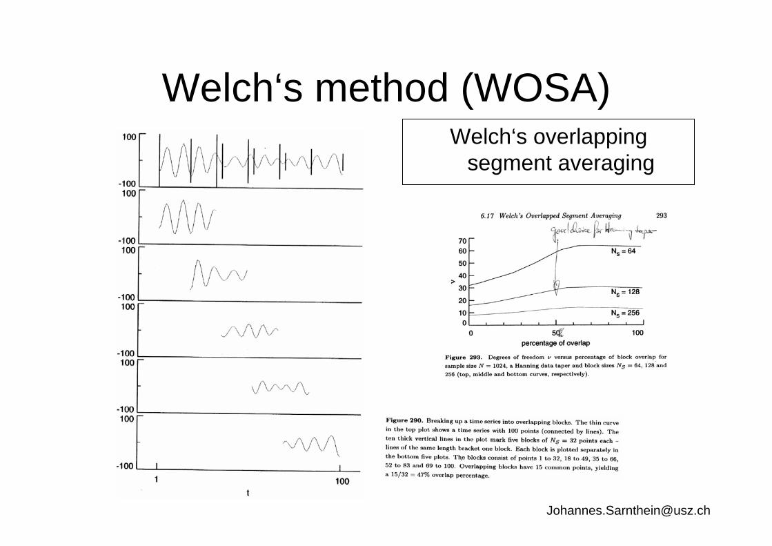
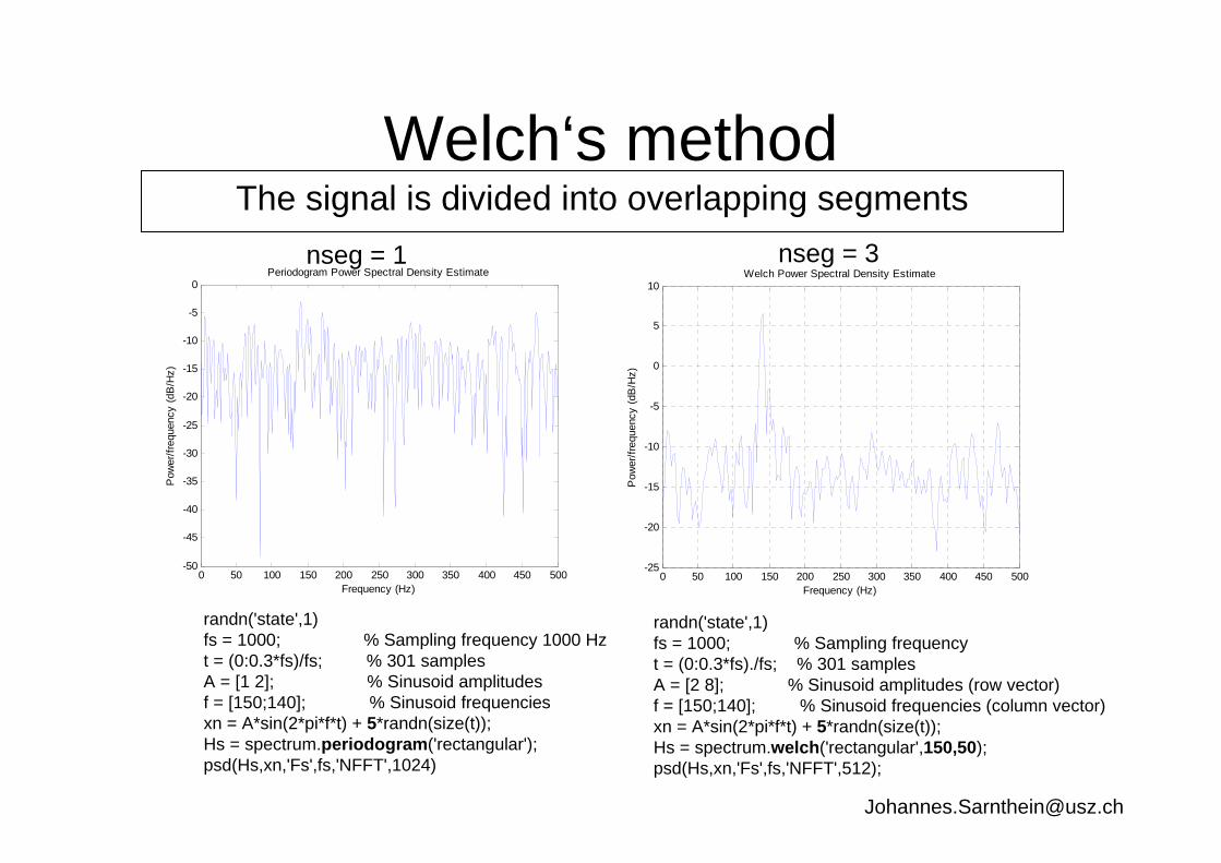
Welch‘s methodThe signal is divided into overlapping segments
randn('state',1)fs = 1000; % Sampling frequency 1000 Hzt = (0:0.3*fs)/fs; % 301 samplesA = [1 2]; % Sinusoid amplitudesf = [150;140]; % Sinusoid frequenciesxn = A*sin(2*pi*f*t) + 5*randn(size(t));Hs = spectrum.periodogram('rectangular');psd(Hs,xn,'Fs',fs,'NFFT',1024)
randn('state',1)fs = 1000; % Sampling frequencyt = (0:0.3*fs)./fs; % 301 samplesA = [2 8]; % Sinusoid amplitudes (row vector)f = [150;140]; % Sinusoid frequencies (column vector)xn = A*sin(2*pi*f*t) + 5*randn(size(t));Hs = spectrum.welch('rectangular',150,50);psd(Hs,xn,'Fs',fs,'NFFT',512);
nseg = 1 nseg = 3
0 50 100 150 200 250 300 350 400 450 500-25
-20
-15
-10
-5
0
5
10
Frequency (Hz)
Pow
er/fr
eque
ncy
(dB
/Hz)
Welch Power Spectral Density Estimate
0 50 100 150 200 250 300 350 400 450 500-50
-45
-40
-35
-30
-25
-20
-15
-10
-5
0
Frequency (Hz)
Pow
er/fr
eque
ncy
(dB
/Hz)
Periodogram Power Spectral Density Estimate

Chi2 Confidence interval
{ }( ){ }
nsegPP
PPE
afP
xx
xx
xx
xx
xx
/1,21
1ˆ
211
ˆvar
ˆ2
)(ˆ
2
2
≈−
≤≤+
=
=
εεε
υ
χυ

34.00209249354920432534
46.0035514998383138543432
37.2043119238544651424
meanBootstrap samples
384142924665313425
2045535515434969
51544298744454493281
Original sample
Bootstrap Confidence intervalhttp:\\people.revoledu.com\kardi\tutorial\bootstrap\


