Estimating and forecasting volatility withlarge scale models: theoretical appraisal of

professionals’ practice

Paolo Zaffaroni ∗

Imperial College London

This draft: 27th April 2006

∗Address correspondence to:Tanaka Business School, Imperial College London, South Kensington Campus, SW7 2AZLondon, tel. + 44 207 594 9186, email p.zaffaroni@imperial.ac.uk

Abstract

This paper examines the way in which GARCH models are esti-mated and used for forecasting by practitioners. Although it permitssizable computational gains and provide a simple way to impose posi-tive semi-definitiveness of multivariate version of the model, we showthat this approach delivers non-consistent parameter’ estimates. Thenovel theoretical result is corroborated by a set of Montecarlo exer-cises. Various empirical applications suggest that this could cause, ingeneral, unreliable forecasts of conditional volatilities and correlations.

Keywords: GARCH, RiskmetricsTM , estimation, forecasting, multivariate volatilitymodels.

2

1 Introduction

Accurate forecasting of volatility and correlations of financial asset returnsis essential for optimal asset allocation, managing portfolio risk, derivativepricing and dynamic hedging. Volatility and correlations are not directlyobservable but can only be estimated using historical data on asset returns.Financial institutions typically face the problem of estimating time-varyingconditional volatilities and correlations for a large number of assets. More-over, fast and computationally efficient methods are required. Therefore,parametric models of changing volatility are those most commonly used,rather than semi- and non-parametric methods. In particular, the autore-gressive conditional heteroskedasticity (ARCH) model of Engle (1982), andthe generalized ARCH (GARCH) of Bollerslev (1986), represent the mostrelevant paradigms. GARCH models are easy to estimate and fit financialdata remarkably well (see Andersen and Bollerslev (1998)). In fact, GARCHmodels do account for several of the empirical regularities of asset returns(see Bollerslev, Engle, and Nelson (1994)), in particular dynamic conditionalheteroskedasticity.

The popularity of GARCH models among practitioners in part stemsfrom their close analogies with linear time series models such as autore-gressive integrated moving average models (ARIMA), as well as with other,a-theoretical, models such as the exponentially weighted moving average(EWMA) model. Precisely by exploiting such analogies has permitted afeasible and computationally fast method for evaluating the conditional time-varying covariance matrix for a large number of assets, of the order of thehundreds. This method, which can be viewed as a highly restricted multivari-ate GARCH, has been popularized under the name of RiskMetrics TM ap-proach (see J.P.Morgan/Reuters (1996)). In this paper we shall call this thecommon approach, acknowledging that it has been the dominant paradigmused by most financial analysts in the last years (see J.P.Morgan/Reuters(1996) and Litterman and Winkelmann (1998)).

Given the widespread evidence of practitioners using the common ap-proach, this paper examines its theoretical underpinnings and effective per-formance. Surprisingly, very little theoretical research has been carried outon this topic. A notable exception is Cheng, Fan, and Spokoiny (2003) whonest the common approach within a wide class of filtering problems. Theyshow that, under mild conditions, the filtering performance of the commonapproach does not depend on whether one uses (observed) square returns

1

rather than the (unobserved) volatility process. This paper focuses insteadon the estimation part of the filtering. Its main contribution is to show howthe estimation method, embedded within the common approach, deliversnon consistent estimates of the model parameters. A Montecarlo exercise de-scribes the finite-sample properties of the estimator, indicating that its poorperformance does not only arise asymptotically. Consequently, misleadingforecasts are likely to occur. More importantly, conditional cross-covariancesand correlations are poorly estimated, possibly leading to unexpected riskexposure when the estimated conditional covariance matrix is used to cal-culate dynamic hedge-ratios, Value-at-Risk performance and mean-varianceefficient portfolios.

The common approach is frequently carried out without preliminaryestimation, with parameters fixed a priori. When a change in the dynamicpattern of the data is likely to occur, calibrated parameters values mustchange accordingly. New estimates are needed in such circumstances andthis is troublesome for the common approach. The impossibility to estimateparameters’ model all depends on the particular, albeit attractively simple,specification that characterizes the common approach.

Adopting the common approach contrasts with the use of correctly spec-ified GARCH models which we will be referring to as the correct approach.Practical applications of the correct approach for large scale problems (in-volving a large number of assets) is limited by the large number of parametersinvolved. As a consequence, the several proposed versions of multivariateGARCH models entail strong forms of parametric simplification, in orderto achieve computational feasibility. Recent advances include the orthogo-nal GARCH model of Alexander (2001), the dynamic conditional correlation(DCC) model of Engle (2002), which generalizes the constant conditional cor-relation model of Bollerslev (1990), the regime-switching DCC of Pelletier(2002) and the averaged conditional correlations of Audrino and Barone-Adesi (2004). Bauwens, Laurent, and Rombouts (2003) provides a completesurvey of this literature.

This paper proceeds as follows. Section 2 presents both the univariatecommon and correct approach. In particular, Section 2.1 describes the wayin which univariate GARCH models are routinely specified and estimated bypractitioners. Section 2.2 recalls the correct specification of GARCH modelsand related estimation issue. Section 2.3 looks at the small-sample propertiesof the estimation nested within the common approach by means of a setof Montecarlo exercises. A comparison of the predictive ability of the two

2

approaches is described in Section 2.4, based on the Olsen’s data set of thespot Mark/Dollar foreign exchange rate. Multivariate models are examinedin Section 3, which also proposes two further empirical illustrations basedon the Olsen’s data set and on the Standard & Poor’s 500 industry indexes.Concluding remarks are in Section 4. Section 5 contains a mathematicalappendix.

2 Univariate case

2.1 Common approach

Let Pt be the speculative price of a generic asset at date t and define thecontinuously compounded one-period rate of return as rt = ln(Pt/Pt−1). Tofocus on the volatility dynamics, assume for the sake of simplicity that thert are martingale differences:

E(rt | Ft−1) = 0, (1)

where Ft defines the sigma-algebra induced by the rs, s ≤ t. The simplestestimator of the conditional variance E(r2

t | Ft−1) = σ2t is the weighted rolling

estimator, with window of length n:

σ2t =

n∑s=1

ws(n)r2t−s (2)

where the weights ws(n) satisfy

ws(n) ≥ 0, limn→∞

n∑s=1

ws(n) = 1,

(see J.P.Morgan/Reuters (1996, Table 5.1) and Litterman and Winkelmann(1998, eq.(1)) among others). σ2

t is a function of n but we will not makethis explicit for simplicity’s sake. Important particular cases of (2) are theequally weighted estimator, for ws(n) = 1/n, and the exponentially weightedestimator, for

ws(n) = (1− λ0) λs−10 , (3)

3

for constant 0 < λ0 < 1, known as the decay factor. The weights (3) yieldthe popular EWMA estimator

σ2t = (1− λ0)

n∑s=1

λs−10 r2

t−s. (4)

The practical appeal of the EWMA estimator (4) lies in the fact that, bysuitably choosing λ0, the estimate will be more sensitive to newer observa-tions than to older observations (cf. J.P.Morgan/Reuters (1996, p.80) andLitterman and Winkelmann (1998, p.15)). Computationally, EWMA is notmore burdensome than simple averages, thanks to the recursion

σ2t = λ0 σ2

t−1 + (1− λ0)r2t−1,

where the initial condition σ2t−n implies another term λn

0 σ2t−n on the right

hand side of (4). For practical implementation,

σ2t =

(1− λ0)

(1− λn0 )

n∑s=1

λs−10 r2

t−s. (5)

is used, rather than (4), ensuring that∑n

s=1 ws(n) = 1 for any finite n. (5)implies the recursion

σ2t = λ0 σ2

t−1 +(1− λ0)

(1− λn0 )

r2t−1 −

(1− λ0)

(1− λn0 )

λn−10 r2

t−n−1.

Typically, the initialization of such recursion is based on the sample varianceof a pre-sample of data. Alternatively, assuming to observe a sample r1, ..., rT

of data and for a given n, one can evaluate (5) for t ≤ n with an expandingwindow (replacing n with t− 1), and returning to (5) when t > n.

When the weights ws(n) vary suitably with n, the rolling estimator, thougha-theoretical, can be justified as a non-parametric estimator of the conditionalvariance. This rules out the possibility that σ2

t nests the EWMA (4) which,however, is closely related to parametric time series models, such as GARCH.The weights of the (rolling) EWMA (23) vary with n but without convergingtowards zero as n grows to infinity, again ruling out the non-parametricinterpretation.

The rt are said to obey the GARCH(1, 1) model when satisfying

rt = ztσt, (6)

σ2t = ω0 + α0r

2t−1 + β0σ

2t−1 a.s. (7)

4

where a.s. stands for almost surely. The zt represent an independent andidentically distributed (i.i.d.) sequence with mean zero and unit variance.Equation (6) then satisfies (1). The coefficients ω0, α0 and β0 must be non-negative for σ2

t to be well defined (cf. Bollerslev (1986)). When

α0 + β0 = 1, (8)

one obtains the integrated GARCH(1, 1) (henceforth IGARCH(1, 1)), by re-placing (7) with

σ2t = ω0 + α0r

2t−1 + (1− α0)σ

2t−1 a.s. (9)

Recursive substitution (n times) in (9) yields

σ2t = ω0

(1− (1− α0)

n−1

α0

)+ (1− α0)

nσ2t−n + α0

n∑s=1

(1− α0)s−1r2

t−s. (10)

Imposingω0 = 0 (11)

IGARCH(1, 1) (10) and EWMA (4) coincide.GARCH have, moreover, a close connection with ARMA (cf. Bollerslev

(1986)). In fact, setting

νt = r2t − σ2

t = (z2t − 1)σ2

t ,

GARCH(1, 1) has an ARMA(1, 1) representation

r2t = ω0 + (α0 + β0)r

2t−1 + νt − β0νt−1.

Note that the νt are martingale differences (not necessarily with finite vari-ance). Under (8) one gets an ARIMA(0, 1, 1)

r2t = ω0 + r2

t−1 + νt − (1− α0)νt−1. (12)

Therefore, the squares r2t display a unit root with non-negative drift. It is

well known that for standard, linear, unit root models, with positive drift,the series diverges a.s. to infinity. This suggested to focus on IGARCH(1, 1)models satisfying (11) (cf. J.P.Morgan/Reuters (1996, eq. (5.37)) and Lit-terman and Winkelmann (1998, eq. (4))).

5

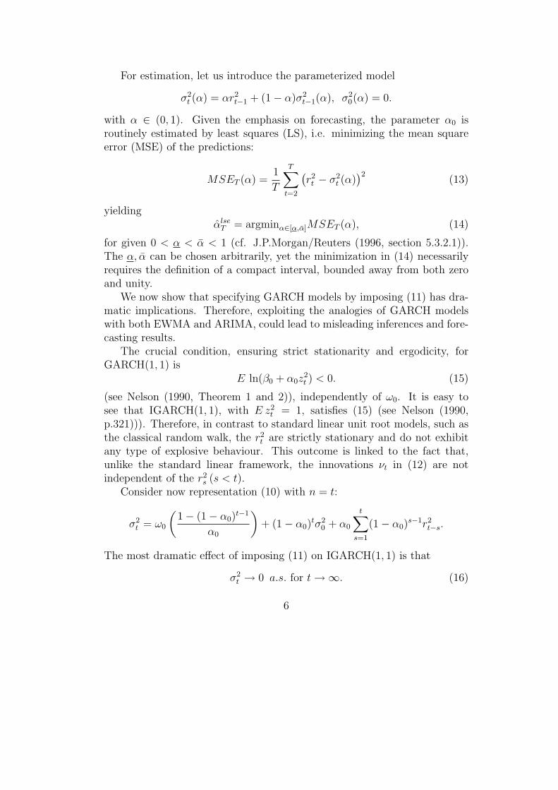
For estimation, let us introduce the parameterized model

σ2t (α) = αr2

t−1 + (1− α)σ2t−1(α), σ2

0(α) = 0.

with α ∈ (0, 1). Given the emphasis on forecasting, the parameter α0 isroutinely estimated by least squares (LS), i.e. minimizing the mean squareerror (MSE) of the predictions:

MSET (α) =1

T

T∑t=2

(r2t − σ2

t (α))2

(13)

yieldingαlse

T = argminα∈[α,α]MSET (α), (14)

for given 0 < α < α < 1 (cf. J.P.Morgan/Reuters (1996, section 5.3.2.1)).The α, α can be chosen arbitrarily, yet the minimization in (14) necessarilyrequires the definition of a compact interval, bounded away from both zeroand unity.

We now show that specifying GARCH models by imposing (11) has dra-matic implications. Therefore, exploiting the analogies of GARCH modelswith both EWMA and ARIMA, could lead to misleading inferences and fore-casting results.

The crucial condition, ensuring strict stationarity and ergodicity, forGARCH(1, 1) is

E ln(β0 + α0z2t ) < 0. (15)

(see Nelson (1990, Theorem 1 and 2)), independently of ω0. It is easy tosee that IGARCH(1, 1), with E z2

t = 1, satisfies (15) (see Nelson (1990,p.321))). Therefore, in contrast to standard linear unit root models, such asthe classical random walk, the r2

t are strictly stationary and do not exhibitany type of explosive behaviour. This outcome is linked to the fact that,unlike the standard linear framework, the innovations νt in (12) are notindependent of the r2

s (s < t).Consider now representation (10) with n = t:

σ2t = ω0

(1− (1− α0)

t−1

α0

)+ (1− α0)

tσ20 + α0

t∑s=1

(1− α0)s−1r2

t−s.

The most dramatic effect of imposing (11) on IGARCH(1, 1) is that

σ2t → 0 a.s. for t →∞. (16)

6

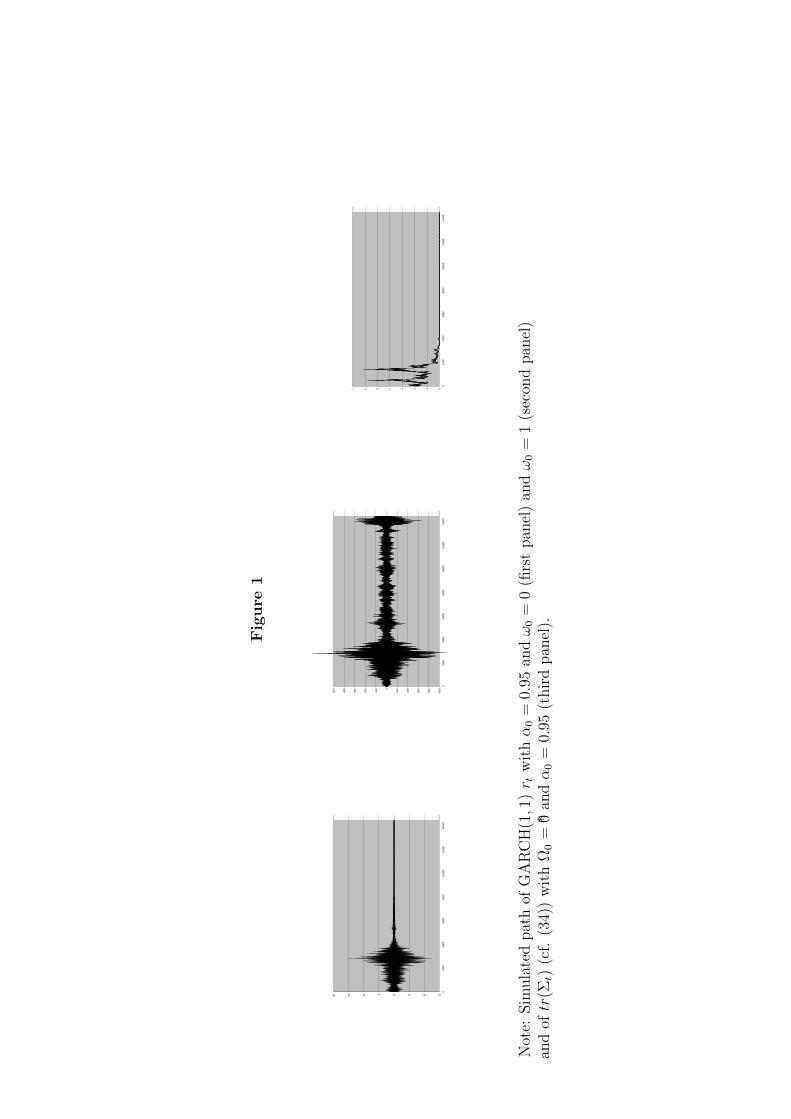
when (11) holds (see Nelson (1990, Theorem 1)). The impact of this resultcan be viewed by means of a simulation, displayed in Figure 1 (left panel),based on setting α = 0.95. It turns out that the smaller α is, the sooner theconditional variance will converge towards zero. Note that once σ2

t = 0 forsome t, then σ2

s = 0, and thus rs+1 = 0 for any s ≥ t, as from (9)

σ2t = σ2

t−1

(α0z

2t−1 + (1− α0)

),

so zero represents an absorption state for the process.This asymptotic degenerateness might, nevertheless, not be important

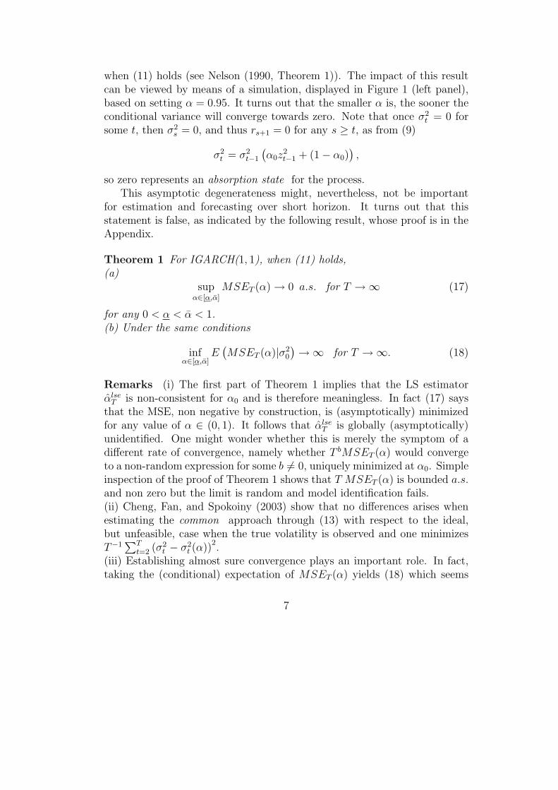
for estimation and forecasting over short horizon. It turns out that thisstatement is false, as indicated by the following result, whose proof is in theAppendix.

Theorem 1 For IGARCH(1, 1), when (11) holds,(a)

supα∈[α,α]

MSET (α) → 0 a.s. for T →∞ (17)

for any 0 < α < α < 1.(b) Under the same conditions

infα∈[α,α]

E(MSET (α)|σ2

0

) →∞ for T →∞. (18)

Remarks (i) The first part of Theorem 1 implies that the LS estimatorαlse

T is non-consistent for α0 and is therefore meaningless. In fact (17) saysthat the MSE, non negative by construction, is (asymptotically) minimizedfor any value of α ∈ (0, 1). It follows that αlse

T is globally (asymptotically)unidentified. One might wonder whether this is merely the symptom of adifferent rate of convergence, namely whether T bMSET (α) would convergeto a non-random expression for some b 6= 0, uniquely minimized at α0. Simpleinspection of the proof of Theorem 1 shows that T MSET (α) is bounded a.s.and non zero but the limit is random and model identification fails.(ii) Cheng, Fan, and Spokoiny (2003) show that no differences arises whenestimating the common approach through (13) with respect to the ideal,but unfeasible, case when the true volatility is observed and one minimizesT−1

∑Tt=2 (σ2

t − σ2t (α))

2.

(iii) Establishing almost sure convergence plays an important role. In fact,taking the (conditional) expectation of MSET (α) yields (18) which seems

7

to contradict Theorem 1. This (apparent) contradiction is a by-product ofthe non stationarity of IGARCH. Basically, the asymptotic behaviour of theaverage of moments does not reflect the asymptotic behaviour of the averageof the underlying random variables. Recall that for IGARCH(1, 1) condition(15) holds.

2.2 Correct approach

Under (15) IGARCH(1, 1) are strictly stationary and ergodic. This impliesthat, despite the ARIMA(0, 1, 1) representation, there is no harm in imposing

ω0 > 0. (19)

Indeed, Nelson (1990, Theorem 2) has shown that under (15) and (19)

σ2t − uσ

2t → 0 a.s. for t →∞,

setting

uσ2t =

ω0

α0

+ α0

∞∑s=1

(1− α0)s−1r2

t−s.

uσ2t defines the unconditional process, in contrast to σ2

t which defines theconditional process as it depends on the initial condition σ2

t−n. Moreover, ithas been shown that the uσ

2t are strictly stationary and ergodic, with a well-

defined non degenerate probability measure on [ω0/α0,∞). Figure 1 (middlepanel), based on setting α = 0.95, provides a typical sample path for theprocess. Now the model conditional variance is always bounded away fromzero and the process is never degenerate. IGARCH(1, 1) are, however, notcovariance stationary. In fact, under (8) the rt have infinite variance althoughthe sample path will not be explosive, thanks to the strict stationarity andergodicity. For this reason, the IGARCH(1, 1) parameters ω0 and α0 cannotbe estimated by LS. However, the model is well specified and can be estimatedin various ways, the most common of which is by pseudo maximum likelihood(PML). The PML estimator (PMLE) is characterized by standard asymptoticstatistical properties (see Lee and Hansen (1994) and Lumsdaine (1996)), andit is given by

(ωpmleT , αpmle

T ) = argminω,α∈[α,α]×[ω,ω] LT (ω, α)

8

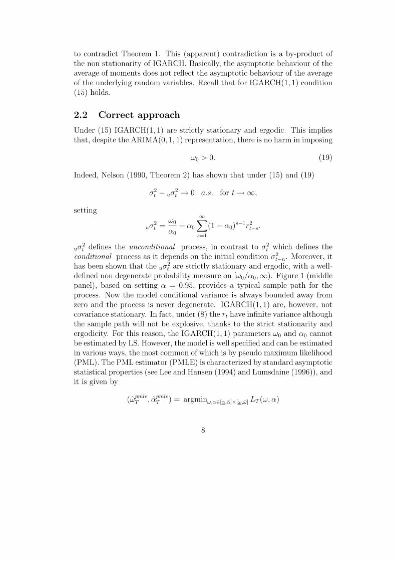
for constants 0 < α < α < 1 and 0 < ω < ω < ∞, setting

LT (ω, α) =1

T

T∑t=1

ln σ2t (ω, α) +

1

T

T∑t=1

r2t

σ2t (ω, α)

(20)

with the parameterized conditional variance

σ2t (ω, α) = ω + αr2

t−1 + (1− α)σ2t−1(ω, α).

2.3 Small-sample performance

Table 1 reports a Montecarlo exercise in order to evaluate the performance ofthe LS estimator αlse

T and of the PMLE αpmleT used, respectively, to estimate

the common and the correct approach. One can also compare the com-mon and the correct approaches using the same estimator, in particular thePMLE. However, we feel that it is more relevant to compare the two modelsusing the corresponding estimation procedure most frequently used by prac-titioners. Moreover, the asymptotic degeneratedness (16) would make theimplementation of the PMLE problematic for the common approach.

Concerning the former, we simulated IGARCH(1, 1) imposing (11), withα0 = 0.05, 0.75 and 0.95. We consider samples of length 15, 000 and es-timate the model considering the first 1, 000 observations, the first 5, 000observations and, lastly, all 15, 000 observations. The MSE is minimized bynumerical methods with a MatLab code, starting from an arbitrary valueequal to 0.5. Such choice should be completely irrelevant for a well speci-fied model. The non-consistency of αlse

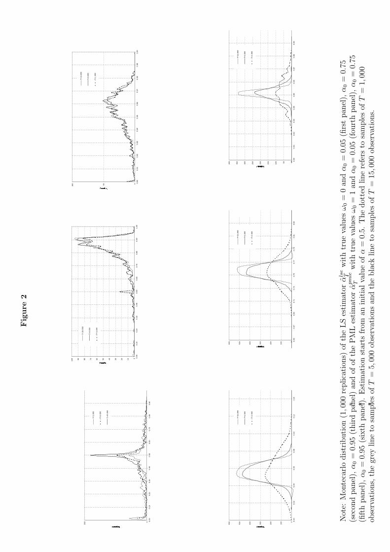
T clearly emerges when comparing theMontecarlo variances (column three) for different sample sizes, which do notvary with T . On the other hand, when looking at the Montecarlo means(column two), it seems that the LS estimator is reliable for large values ofα0. (For case α0 = 0.05 also the mean indicates the non consistency). Thesenumerical results can be better evaluated by looking at the Montecarlo fre-quency distributions of the LS estimator, reported in Figure 2 (top threepanels). It clearly appears that the LS estimator is both non-consistent andnon-centered (biased) with respect to the true value. Interestingly, note howthe behaviour of the LS estimator for case α0 = 0.95 (top right panel) isheavily influenced by the initial, very persistent, observations. As a result,the estimate is close to the true value although in reality this is independentof its asymptotic statistical properties. It is thus possible that a mis-specified

9

model achieves a good forecasting performance. This possibility is investi-gated in section 2.4.

Columns seven to twelve of Table 1 report the small-sample properties ofthe PMLE, based on samples of size T = 1, 000, 5, 000 and 15, 000. Again theoptimization started from the same arbitrary value of 0.5 for α. The estimatesare all centered around the true value and their variance decreases as thesample size increases, at rate 1/T . The average of (20) across replications,evaluated at the PMLE (column twelve of Table 1), does not significantlychange with T . The empirical distribution of the estimates are reported inFigure 2 (bottom three panels).

2.4 Comparing forecasting performances (univariate)

Our theoretical result indicates the inherent difficulties for estimation of thecommon approach. We now present a simple empirical application aimedat providing some evidence on the forecasting implications of the theoreticalresult.

We compare the predictive capability of IGARCH(1, 1) models describedin section 2.1 and 2.2, that is with and without condition (11). Hereafter,we denote the former as model 2 and the latter as model 1. We consider theDiebold and Mariano (1995) test of predictive accuracy

DMS(L) =1√AS

S∑s=1

(L(σ2

s ,(1)σ2

s|s−p)− L(σ2s ,

(2)σ2s|s−p)

)(21)

where S defines the number of p-step ahead forecasts employed and L(a, b)defines a generic loss function. (1)σ2

s|s−p and (2)σ2s|s−p express the two, compet-

ing, p-step ahead forecasts of the true conditional volatility σ2s . The normal-

izing quantity AS is a consistent estimate of the variance of the numerator of(21), robust to autocorrelation of unknown form (see Diebold and Mariano(1995, section 1.1) for details), such that under suitable regularity conditionsDMS(L) converges in distribution to a standard normal (for S →∞ ), underthe null hypothesis of equal forecasting performance

E(L(σ2

s ,(1)σ2

s|s−p)− L(σ2s ,

(2)σ2s|s−p)

)= 0.

We employ the well-known data set of Olsen & Ass., frequently used to com-pare predictive performance of volatility models since Andersen and Boller-slev (1998). In particular, the data consist of daily and intra-daily returns

10

for the Mark/Dollar spot exchange rate (henceforth Mark/Dollar returns),from July 1, 1974, through September 30, 1992 - 4, 573 observations - fordaily data, and from October 1, 1992, through September 30, 1993 - 74, 880observations - for intra-daily data (five-minute returns). We then obtain 260observations of the so-called realized volatility, obtained by summing squaredintra-daily returns (288 intra-daily observations per day), as indicated by An-dersen and Bollerslev (1998). In this exercise we assume that the realizedvolatility expresses true (daily) volatility, denoted by σ2

t , with a negligibleerror.

The results are reported in Table 2. The data in levels (returns) havebeen preliminary filtered with an AR(1) model. The two volatility modelsare then estimated, first, using 4, 573 daily observations, then 4, 573 + 1observations, and so on up to 4, 573 + 259 observations. West (1996) notedthat the asymptotic distribution of DMS(L) might depend on the samplevariability of parameter estimates. However he established that no effectarises when the length of the estimation sample dominates the length of theevaluation sample. Since in our case the former (4, 573) is nearly twenty timesthe latter (260), we proceed ignoring the effect of parameter uncertainty. Theaverages of the 260 different point estimates of α0 for both models (estimatesof ω0 for model 1 are not reported for the sake of simplicity) are reportedin column two and column three for model 2 and model 1 respectively. Forboth models estimation starts from an initial value α = 0.95.

We consider two different types of loss function, the square-rooted ab-solute difference L(a, b) =| a − b | 12 and the loss function implicit in theGaussian log likelihood L(a, b) = ln(b) + a/b (see Bollerslev, Engle, and Nel-son (1994, section 7)), whose results are reported in columns 4−7 and 8−11respectively. Four different forecasting horizons are considered: at 1 day, 1week, 1 month and 6 months ahead. The forecasting function for model 1(correctly specified IGARCH(1, 1), without imposing (11)), is

(1)σ2t+p|t = E((1)σ2

t+p|Ft) = pω0 + α0r2t + (1− α0)σ

2t .

For model 2 (degenerate IGARCH(1, 1), imposing (11)) the forecast functionis constant and equal to

(2)σ2t+p|t = E((2)σ2

t+p|Ft) = α0r2t + (1− α0)σ

2t ,

for any p ≥ 1. Obviously the preceding expressions are in practice evalu-ated at the estimated, rather than true, parameter values. The choice made

11

for the loss functions reflects the estimation methods employed for model 1and model 2 respectively. The square-rooted absolute difference loss func-tion should potentially favor model 2 whereas the Gaussian likelihood lossfunction should favor model 1. Comparing the results for the two loss func-tions should avoid biases when assessing the forecasting performance of thecompeting models.

There are two main findings. First, the forecasting performance of model2 is significantly worse than that of model 1 in most cases, or at most notsignificantly different from it, for short and medium-run horizons (1 day, 1week and 1 month). By contrast, for longer horizon (6 months), model 2outperforms model 1 for the square-root loss function and it is not signifi-cantly different from model 2 for the Gaussian loss function. This outcome isnot completely surprising. In fact, the asymptotic degenerateness of model 2implies a well-behaved forecasting function for all horizons, whereas for (thecorrectly specified) model 1 the forecasting function diverges to infinity, asthe forecast horizon grows to infinity.

Second, the forecasting performance of model 2 is extremely dependenton the initial value for σ2

0(α) chosen when estimating the model. The firstfour rows of Table 2 refer to different values for σ2

0(α), all arbitrarily chosen,except for row four for which σ2

0(α) has been estimated jointly with α. Nev-ertheless, even for this last case, the poor forecasting performance of model2 emerges (except for the long horizon). In fact, different initial conditionsimply extremely different point estimates for α, as indicated in the secondcolumn reporting the average of the αlse

T , and thus different forecasts. Theperformance of the two models is comparable when setting σ2

0(α) = 0.1 inthe estimation of model 2, yielding an average of the αlse

T equal to 0.881,not surprisingly close to the average of the αpmle

T of 0.851. Clearly, findingex-ante a good value for σ2

0(α), to estimate model 2, is not an attainabletask in general. This should not, and in fact is not, an issue for the correctapproach, with the effect of initial conditions being asymptotically negligi-ble. The last three rows report the result obtained setting σ2

0(α) equal tothe sample variance of the data, and setting α = 0.94. This is the valuesuggested by J.P.Morgan/Reuters (1996, p.100) and, presumably, close by toany other values used by practitioners. The last two rows consider the rollingEWMA (eq.(5)) with n = 15, 30 whereas row five considers the expandingwindow n = t − 1. For these case as well, no significative difference arisesbetween the two competing models for all but the 6 months horizon.

12

3 Multivariate case

Typical situations faced by practitioners, such as optimal asset allocationsand portfolio risk diversification, involve many assets. For instance, J.P.Morgan/Reuters(1996, p.97) considers the problem of estimating the conditional covariancematrix of 480 time series. In such circumstances, as discussed in Section 1,use of correctly specified (unrestricted) multivariate GARCH models is nota possibility and some form of restrictions are required in order to achievecomputational feasibility. The common approach, instead, is always appli-cable in such situations, which motivates its widespread use for real timeapplications. Note that implementation and estimation of the multivariatecommon approach heavily relies on the results derived for univariate case,fully described in Section 2.1.

3.1 Common approach

Assuming that (1) holds for each asset and that there are m assets, the rollingestimator for the conditional covariance between the returns of asset i andasset j is

σij,t =n∑

s=1

ws(n)ri,t−srj,t−s, i, j = 1, ..., m, (22)

where ri,t = ln(Pi,t/Pi,t−1) and Pi,t denotes the speculative price of asset i(see J.P.Morgan/Reuters (1996, Table 5.4) and Litterman and Winkelmann(1998, eq. (2))). Likewise, the EWMA is

σij,t = (1− λ0)n∑

s=1

λs−10 ri,t−srj,t−s, (23)

whose recursive form is

σij,t = λ0σij,t−1 + (1− λ0)ri,t−1rj,t−1, σij,t−n = 0. (24)

Note that the parameter λ0 does not vary with i, j and, indeed, this choiceguarantees that the m×m matrix Σt = [σij,t] (1 ≤ i, j ≤ m), solution of

Σt = λ0Σt−1 + (1− λ0)rt−1r′t−1, Σ0 = 0,

13

is positive semi-definite, setting rt = (r1,t, ..., rm,t)′ (cf. J.P.Morgan/Reuters

(1996, p. 97)). Practical implementation of (23) is often based on

σij,t =(1− λ0)

(1− λn0 )

n∑s=1

λs−10 ri,t−srj,t−s, (25)

with the recursion (in matrix notation)

Σt = λ0Σt−1 +(1− λ0)

(1− λn0 )

rt−1r′t−1 −

(1− λ0)

(1− λn0 )

λn−10 rt−n−1r

′t−n−1, (26)

with the same initialization issues of the univariate case as discussed aftereq. (5).

First we establish the analogy of EWMA (23) with multivariate GARCH(1, 1).The latter, in its most general specification, is

rt = Σ12t zt, (27)

vech(Σt) = Ω0 + A0vech(Σt−1) + B0vech(rt−1r′t−1), (28)

where vech(.) denotes the column stacking operator of the lower portion ofa symmetric matrix, zt = (z1,t, ..., zm,t)

′ is an m-valued i.i.d. sequence withEzt = 0 and Eztz

′t = Im where Im is the identity matrix of dimension m×m,

Ω0 is an m(m + 1)/2× 1 vector and A0, B0 are m(m + 1)/2×m(m + 1)/2matrices of coefficients (see Bollerslev, Engle, and Wooldridge (1988, eq. 4)).An appealing feature of (28) is that it produces time-varying conditionalcorrelations, given by (at the one-step-ahead horizon)

ρij,t =E(ri,trj,t | Ft−1)√

E(r2i,t | Ft−1)E(r2

j,t | Ft−1)=

σij,t

σi,tσj,t

, (29)

assuming that (1) holds.Imposing diagonality and constancy of the diagonal terms of A0, B0

yieldsA0 = α0Im(m+1)/2, B0 = β0Im(m+1)/2.

Further imposing (8), one obtains the multivariate IGARCH(1, 1):

σij,t = ωij,0 + α0ri,t−1rj,t−1 + (1− α0)σij,t−1, i, j = 1, ...,m. (30)

14

Despite the ri,t are not covariance stationary, the conditional correlations ρij,t

are well defined. Finally, imposing

ωij,0 = 0, i, j = 1, ...,m, (31)

andσij,t−n = 0, i, j = 1, ..., m, (32)

the EWMA (24) and the multivariate IGARCH(1, 1) (30) coincide. In matrixnotation, the latter is

rt = Σ12t zt, (33)

Σt = α0rt−1r′t−1 + (1− α0)Σt−1. (34)

Substituting (33) into (34) yields

Σt = Σ12t−1At−1Σ

12t−1, (35)

setting At = (α0Im + (1− α0)ztz′t). From (35) it follows that when Σt = 0

then Σs = 0 and rs = 0 for any s > t, in analogy with the univariate case,suggesting that

tr(Σt) → 0 a.s. for t →∞, (36)

where tr(·) is the trace operator. The right panel of Figure 1 reports theresults of a simulation exercise showing that (36) really does occur.

As for the univariate case, the asymptotic degenerateness of the processcauses numerous problems. First, note that when (31) is imposed, the condi-tional correlations (29) are no longer well-defined. For estimation purposes,one can generalize the procedure of section 2.1, and estimate α0 by minimiz-ing the multivariate MSE

αlseT = argminα∈[α,α]

1

T

T∑t=2

‖ rtr′t −Σt(α) ‖2

settingΣt(α) = (1− α)Σt−1(α) + αrt−1r

′t−1, Σ0(α) = 0,

where ‖ · ‖ indicates the Euclidean norm.However, rather than using the LS estimator αlse

T , practitioners adopt atwo-stage approach. First, they estimate univariate EWMA for each asset

15

by minimizing the univariate MSE (cf. (13)), yielding αlse,(i)T (i = 1, ..., m).

They then estimate α0 by a weighted average of the former, yielding

αT =m∑

i=1

φ(i)T α

lse,(i)T ,

with weights that penalize assets whose estimated coefficients have a largeMSE:

φ(i)T =

(θ(i)T )−1

∑mj=1(θ

(j)T )−1

, i = 1, ..., m,

setting

θ(i)T =

√MSET (α

(i)T )√

MSET (α(1)T ) + ... +

√MSET (α

(m)T )

, i = 1, ...,m,

(see J.P.Morgan/Reuters (1996, section 5.3.2.2)).As for the univariate case, it turns out that (31) implies that neither

αlseT nor the frequently used αT is consistent for α0. Concerning the latter,

Theorem 1 applies directly since αT is a weighted average of m estimates ofα0, each of which being non-consistent, and whose weights φi

T converge toa random limit as T → ∞. An additional drawback of αT is that it is, byconstruction, completely independent of the information stemming from theconditional cross-correlations characterizing the data.

3.2 Comparing forecasting performances (multivariate)

This section compares the predictive performance of the common approachversus the correct approach in a multivariate setting. We illustrate a bivari-ate (m = 2) and a medium-scale multivariate (m = 22) exercise. Given ouremphasis on the theoretical result, we mirror section 2.4 and adopt a statisti-cal approach rather than a decision-theoretic approach to forecast evaluation,such as in Pesaran and Zaffaroni (2004).

Regarding the bivariate specification, we employ the Mark/Dollar spotexchange rate series described in section 2.4 as well as the time series ofthe Yen/Dollar spot exchange rate. (The data are described in Andersenand Bollerslev (1998).) Considering only the observations which share thesame trading periods yields 4, 573 daily observations - from July 1, 1974,

16

through September 30, 1992 - and 74, 304 intra-daily (five-minute returns)observations - from October 1, 1992, through September 30, 1993. Table 3describes the results. The return data have been first filtered with an AR(1)model. For this bivariate exercise we consider the loss functions

L1(A,B) =| a11 − b11 | 12 + | a22 − b22 | 12 + | a12 − b12 | 12 ,L2(A,B) =| a12/

√a11a22 − b12/

√b11b22 |,

for any pair of 2× 2 symmetric matrices

A =

(a11 a12

a12 a22

), B =

(b11 b12

b12 b22

).

The first type of loss function generalizes the square-rooted absolute differ-ence used in section 2.4. The second type of loss function compares (condi-tional) cross-correlations. The forecasting function for model 1 is, for p ≥ 1,

(1)Σt+p|t = pΩ0 + α0rtr′t + (1− α0)Σt.

As for the univariate case, the forecast function of model 2 is constant andequal to

(2)Σt+p|t = α0rt r′t + (1− α0)Σt,

for any p. The results of Table 3 confirm that model 1 significantly out-performs model 2 in most cases. The results are less conclusive for longerhorizons. The better performance of model 1 is particularly evident whencomparing conditional cross-correlations (columns 8 − 11). This has impli-cations when one uses multivariate GARCH models to construct optimal(dynamic) hedge-ratios, so as to minimize portfolio risk. Second, we find theextreme sensibility of the estimates and forecasting performance of model2 from initial conditions Σ0(α) = σ2

0(α)I2. Again, the performance of thetwo models is never significantly different when σ2

0(α) = 0.1. When deriv-ing σ0(α) jointly with αT , the performance of model 2 is significantly worsethan that of model 1 for most cases. Finally, note that the estimates αT areonly marginally different from αlse

T , as reported in Table 2. (In both cases,estimation started from α = 0.95.) This is, again, a by-product of the poorstatistical properties of the LS estimator. No significative differences arisewhen calibrating model 2 with α = 0.94 and setting Σ0(α) equal to the sam-ple covariance matrix of the data. Summarizing, when comparing variancesand the covariance, the results are very much similar to the univariate case

17

of Table 2. However, when comparing conditional correlations, the commonapproach never outperforms the correct when λ0 is calibrated. The commonapproach is markedly inferior, at all horizons, when the smoothing parameteris estimated.

For the multivariate exercise, we shall consider the 22 main industry in-dices of the Standard & Poor’s 500 (source: Datastream) extracted fromthe S&P 500 industry price indices defined according to the Global IndustryClassification Standard. Our data set covers the industry indices from 2ndJanuary 1995 to 13th October 2003 (T = 2291 observation). Daily returnsare computed as rjt = 100 ln (Pjt/Pjt−1) , j = 1, ..., 22, where Pjt is the jth

price index. (For a description of the data, and of their statistical properties,we refer to Pesaran and Zaffaroni (2004).) We considered the generaliza-tion of the loss function L1(A,B) in (37) to 22 × 22 matrices, comparingrit+prjt+p, i, j = 1, ..., 22, with their forecast based on the (i, j)th entry of(1)Σt+p|t. Returns have not been preliminary filtered with an AR(1) modelsince negligible time variation of the conditional mean is documented. Un-like the univariate and bivariate examples, it is unfeasible to estimate a well-specified (unrestricted) GARCH model of dimension 22×22 such as (27)-(28).The dynamic conditional correlation (DCC) of Engle (2002) and its asym-metric variation, namely the asymmetric DCC (ADCC) of Cappiello, Engle,and Sheppard (2002), appear superior at describing the dynamic propertiesof this data set, when compared with many other multivariate GARCH-type specifications (see Pesaran and Zaffaroni (2004)). We recall that theDCC(r,s,R,S) implies (1)Σt = DtRtDt for a diagonal matrix Dt, with a(square-rooted) GARCH(r, s) on the (i, i)th entry, and, considering a simplespecification (R=S =1), Rt has qhjt/

√qhht qjjt in its (h, j)th position, setting

Qt = [qhjt]22h,j=1 for

Qt = Q (1− γ0 − δ0) + γ0rt−1r′t−1 + δ0Qt−1,

rt = D−1t rt, a positive definite matrix Q and positive parameters satisfying

0 < γ0+δ0 < 1. The DCC(r, s, 1, 1) and the ADCC(r, s, 1, 1), for 1 ≤ r, s ≤ 2,are compared with the common approach method (26) with λ0 = 0.94, overthe horizon p = 1, 5, 20, 120. Derivation of (1)Σt+p|t for DCC and ADCCis straightforward and details are skipped for sake of simplicity. All modelswere estimated recursively using an expanding window starting with 1784observations as the first estimation sample. The evaluation sample covers thelast two years of data (from November 2, 2001 to October 13, 2003, inclusive)

18

yielding 507−p values for the loss function. However, the parameter valuesare updated at monthly intervals, yielding twenty-four set of estimates ratherthan 507−p, in order to alleviate the already sizeable computational burden.The estimates are nor reported for sake of simplicity. All the computationshave been carried out in MatLab and the codes are available upon request.Compared with the bivariate case, the results, reported in Table 4, now showmore clearly that the correct approach (here represented by DCC and ADCCmodels), is markedly superior to the common approach (RiskmetricsTM) forall cases and all horizon.

4 Concluding remarks

Practitioners face the problem of estimating in real time conditional volatil-ities and cross-correlations for a large set of asset returns. The so-calledcommon approach of specifying, estimating and forecasting GARCH mod-els provides a simple and feasible way to achieve this task. Unfortunately,as this paper shows, the estimates obtained in this way lack of the usual(asymptotic) statistical properties. The Monte-Carlo experiments indicatesthat such estimation procedure is invalid even in small-sample. The empiri-cal applications here presented suggest that this can have a non trivial effecton the forecasting performance of conditional variances and correlations.

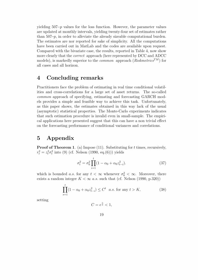
5 Appendix

Proof of Theorem 1. (a) Impose (11). Substituting for t times, recursively,r2t = z2

t σ2t into (9) (cf. Nelson (1990, eq.(6))) yields

σ2t = σ2

0

t∏i=1

(1− α0 + α0z2t−i). (37)

which is bounded a.s. for any t < ∞ whenever σ20 < ∞. Moreover, there

exists a random integer K < ∞ a.s. such that (cf. Nelson (1990, p.320))

t∏s=1

(1− α0 + α0z2t−i) ≤ Ct a.s. for any t > K, (38)

settingC = e

γ2 < 1,

19

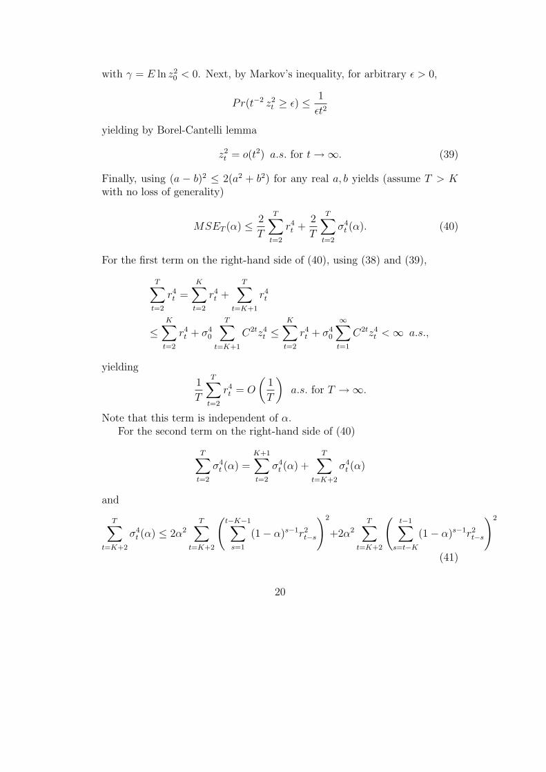
with γ = E ln z20 < 0. Next, by Markov’s inequality, for arbitrary ε > 0,

Pr(t−2 z2t ≥ ε) ≤ 1

εt2

yielding by Borel-Cantelli lemma

z2t = o(t2) a.s. for t →∞. (39)

Finally, using (a − b)2 ≤ 2(a2 + b2) for any real a, b yields (assume T > Kwith no loss of generality)

MSET (α) ≤ 2

T

T∑t=2

r4t +

2

T

T∑t=2

σ4t (α). (40)

For the first term on the right-hand side of (40), using (38) and (39),

T∑t=2

r4t =

K∑t=2

r4t +

T∑t=K+1

r4t

≤K∑

t=2

r4t + σ4

0

T∑t=K+1

C2tz4t ≤

K∑t=2

r4t + σ4

0

∞∑t=1

C2tz4t < ∞ a.s.,

yielding

1

T

T∑t=2

r4t = O

(1

T

)a.s. for T →∞.

Note that this term is independent of α.For the second term on the right-hand side of (40)

T∑t=2

σ4t (α) =

K+1∑t=2

σ4t (α) +

T∑t=K+2

σ4t (α)

and

T∑t=K+2

σ4t (α) ≤ 2α2

T∑t=K+2

(t−K−1∑

s=1

(1− α)s−1r2t−s

)2

+2α2

T∑t=K+2

(t−1∑

s=t−K

(1− α)s−1r2t−s

)2

(41)

20

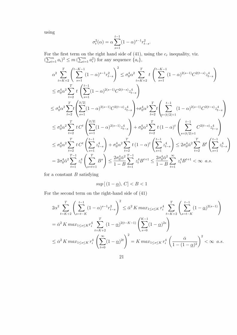
using

σ2t (α) = α

t−1∑s=1

(1− α)s−1r2t−s.

For the first term on the right hand side of (41), using the cr inequality, viz.(∑m

i=1 ai)2 ≤ m (

∑mi=1 a2

i ) for any sequence ai,

α2

T∑t=K+2

(t−K−1∑

s=1

(1− α)s−1r2t−s

)2

≤ σ40α

2

T∑t=K+2

t

(t−K−1∑

s=1

(1− α)2(s−1)C2(t−s)z4t−s

)

≤ σ40α

2

T∑t=2

t

(t−1∑s=1

(1− α)2(s−1)C2(t−s)z4t−s

)

≤ σ40α

2

T∑t=2

t

|t/2|∑s=1

(1− α)2(s−1)C2(t−s)z4t−s

+σ4

0α2

T∑t=2

t

t−1∑

s=|t/2|+1

(1− α)2(s−1)C2(t−s)z4t−s

≤ σ40α

2

T∑t=2

t Ct

|t/2|∑s=1

(1− α)2(s−1)z4t−s

+ σ4

0α2

T∑t=2

t (1− α)t

t−1∑

s=|t/2|+1

C2(t−s)z4t−s

≤ σ40α

2

T∑t=2

t Ct

(t−1∑s=1

z4t−s

)+ σ4

0α2

T∑t=2

t (1− α)t

(t−1∑s=1

z4t−s

)≤ 2σ4

0α2

T∑t=2

Bt

(t−1∑s=1

z4t−s

)

= 2σ40α

2

T−1∑t=1

z4t

(T∑

s=t+1

Bs

)≤ 2σ4

0α2

1−B

T−1∑t=1

z4t B

t+1 ≤ 2σ40α

2

1−B

∞∑t=1

z4t B

t+1 < ∞ a.s.

for a constant B satisfying

sup [ (1− α), C] < B < 1

For the second term on the right-hand side of (41)

2α2

T∑t=K+2

(t−1∑

s=t−K

(1− α)s−1r2t−s

)2

≤ α2 K max1≤s≤K r4i

T∑t=K+2

(t−1∑

s=t−K

(1− α)2(s−1)

)

= α2 K max1≤s≤Kr4i

T∑t=K+2

(1− α)2(t−K−1)

(K−1∑s=0

(1− α)2s

)

≤ α2 K max1≤s≤K r4i

( ∞∑t=0

(1− α)2t

)2

= K max1≤s≤K r4i

(α

1− (1− α)2

)2

< ∞ a.s.

21

Finally, collecting terms

supα∈[α,α]

2

T

T∑t=2

σ4t (α) = O

(1

T

)a.s. for T →∞. 2

(b)

E(MSET (α) | σ20) = T−1

T∑t=1

(E(r4

t | σ20) + E(σ4

t (α) | σ20)− 2E(r2

t σ2t (α) | σ2

0)).

Easy calculations yieldE(r4

t | σ20) = σ4

0δt0

settingδ0 := E(1− α0 + α0z

2t )

2.

Next

E(σ4t (α) | σ2

0)

= α2

t−1∑j=1

(1− α)2(j−1)E(r4t−j | σ2

0) + 2α2

t−2∑j2=1

(1− α)j2−1

t−1∑j1=j2+1

(1− α)j1−1E(r2t−j1

r2t−j2

| σ20)

= σ40α

2

t−1∑j=1

(1− α)2(j−1)δt−j0 + 2σ4

0α2κ0

t−2∑j2=1

(1− α)j2−1

t−1∑j1=j2+1

(1− α)j1−1δt−j10

settingκ0 := E(1− α0 + α0z

2t )z

2t ,

and

E(r2t σ

2t (α) | σ2

0) = κ0α

t−1∑j=1

(1− α)(j−1)δt−j0 .

Tedious calculations yield

E(r4t | σ2

0) + E(σ4t (α) | σ2

0)− 2E(r2t σ

2t (α) | σ2

0) = δt0ct(α),

where the sequence of positive constants ct(α) satisfy ct(α) → c(α) < ∞ as t →∞, setting

c(α) =

(1 +

α2

(δ0 − (1− α)2)+

2α2κ0(1− α)

(δ0 − (1− α))(δ0 − (1− α)2)− 2ακ0

(δ0 − (1− α))

).

22

Note that ct(α), c(α) depend also on δ0, κ0 but we are not making this explicitfor simplicity. By simple manipulations, noting that δ0 = 1+α2

0(µ4−1), κ0 =1 + α0(µ4 − 1) for µ4 := Ez4

0 , one gets

c(α) =α(µ4 − 1)2

(δ0 − (1− α)2)(δ0 − (1− α)),

implyinginf

α∈[α,α]c(α) = c > 0.

Hence (18) easily follows since δ0 > 1. 2

References

Alexander, C. (2001): “Orthogonal GARCH,” in Mastering risk, ed. byC. Alexander, vol. 2, pp. 21–38. London: Financial Times - Prentice Hall.

Andersen, A., and T. Bollerslev (1998): “Answering the skeptics: Yes,standard volatility models do provide accurate forecasts,” InternationalEconomic Review, 39, 885–905.

Audrino, F., and G. Barone-Adesi (2004): “Average conditional corre-lation and tree structures for multivariate GARCH models,” University ofLugano, Preprint.

Bauwens, L., S. Laurent, and J. Rombouts (2003): “MultivariateGARCH models: a survey,” CORE , Preprint.

Bollerslev, T. (1986): “Generalized autoregressive conditional het-eroskedasticity,” Journal of Econometrics, 31, 302–327.

(1990): “Modelling the coherence in short-run nominal exchangerates: a multivariate generalized ARCH,” Review of Economics and Statis-tics, 72, 498–505.

Bollerslev, T., R. Engle, and D. Nelson (1994): “ARCH models,”in Handbook of Econometrics vol. IV, ed. by R. Engle, and D. McFadden.Amsterdam: North Holland.

23

Bollerslev, T., R. Engle, and J. Wooldridge (1988): “A capitalasset pricing model with time varying covariances,” Journal of PoliticalEconomy, 96, 116–131.

Cappiello, L., R. Engle, and K. Sheppard (2002): “Asymmetric dy-namics in the conditional correlations of global equity and bond returns,”NYU, Preprint.

Cheng, M., J. Fan, and V. Spokoiny (2003): “Dynamic nonparametricfiltering with application to finance,” Weiesestrass Insitute and HumboldtUniversity Berlin, Preprint.

Diebold, F., and R. Mariano (1995): “Comparing predictive accuracy,”Journal of Business and Economic Statistics, 13, 253–263.

Engle, R. (2002): “Dynamic conditional correlation - a simple class of mul-tivariate generalized autoregressive conditional heteroskedasticity mod-els,” Journal of Business & Economic Statistics, 20, 339–350.

Engle, R. F. (1982): “Autoregressive conditional heteroskedasticity withestimates of the variance of the United Kingdom,” Econometrica, 50, 987–1007.

J.P.Morgan/Reuters (1996): “RiskMetricsTM - Technical Document,Fourth Edition,” .

Lee, S., and B. Hansen (1994): “Asymptotic theory for the GARCH(1,1)quasi-maximum likelihood estimator,” Econometric Theory, 10, 29–52.

Litterman, R., and K. Winkelmann (1998): “Estimating CovarianceMatrices,” Risk management series, Goldman Sachs & Co.

Lumsdaine, R. (1996): “Consistency and asymptotic normality of thequasi-maximum likelihood estimator in IGARCH(1,1) and covariance sta-tionary GARCH(1,1) models,” Econometrica, 64/3, 575–596.

Nelson, D. (1990): “Stationarity and persistence in the GARCH(1,1)model,” Econometric Theory, 6, 318–334.

Pelletier, D. (2002): “Regime switching for dynamic correlations,” Jour-nal of Econometrics, forthcoming.

24

Pesaran, M., and P. Zaffaroni (2004): “Model Averaging and Value-at-Risk based Evaluation of Large Multi Asset Volatility Models for RiskManagement,” University of Cambridge, Preprint.

West, K. (1996): “Asymptotic inference about predictive ability,” Econo-metrica, 64, 1067–1084.

25

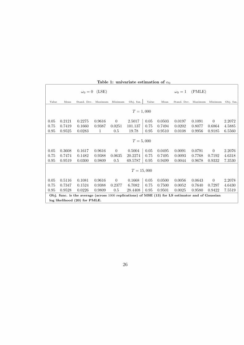
Table 1: univariate estimation of α0

ω0 = 0 (LSE) ω0 = 1 (PMLE)

Value Mean Stand. Dev. Maximum Minimum Obj. fun. Value Mean Stand. Dev. Maximum Minimum Obj. fun.

T = 1, 000

0.05 0.2121 0.2275 0.9616 0 2.5017 0.05 0.0503 0.0197 0.1091 0 2.20720.75 0.7419 0.1660 0.9387 0.0251 101.137 0.75 0.7494 0.0202 0.8077 0.6864 4.58850.95 0.9525 0.0283 1 0.5 19.78 0.95 0.9510 0.0108 0.9956 0.9185 6.5560

T = 5, 000

0.05 0.3608 0.1617 0.9616 0 0.5004 0.05 0.0495 0.0091 0.0791 0 2.20760.75 0.7474 0.1482 0.9388 0.0635 20.2274 0.75 0.7495 0.0093 0.7768 0.7192 4.63180.95 0.9519 0.0300 0.9809 0.5 69.5787 0.95 0.9499 0.0044 0.9678 0.9332 7.3530

T = 15, 000

0.05 0.5116 0.1081 0.9616 0 0.1668 0.05 0.0500 0.0056 0.0643 0 2.20780.75 0.7347 0.1524 0.9388 0.2377 6.7082 0.75 0.7500 0.0052 0.7640 0.7297 4.64300.95 0.9528 0.0226 0.9809 0.5 28.4408 0.95 0.9501 0.0025 0.9580 0.9422 7.5519Obj. func. is the average (across 1000 replications) of MSE (13) for LS estimator and of Gaussian

log likelihood (20) for PMLE.

26

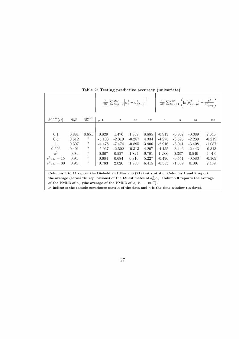
Table 2: Testing predictive accuracy (univariate)

1260

∑260t=p+1

∣∣∣σ2t − σ2

t|t−p

∣∣∣12 1

260

∑260t=p+1

(ln(σ2

t|t−p) + σ2t

σ2t|t−p

)

σ2,lse0 (α) αlse

T αpmleT p: 1 5 20 120 1 5 20 120

0.1 0.881 0.851 0.829 1.476 1.958 8.885 -0.913 -0.957 -0.389 2.6450.5 0.512 ” -5.103 -2.319 -0.257 4.334 -4.275 -3.595 -2.239 -0.2191 0.307 ” -4.478 -7.474 -0.895 3.906 -2.916 -3.041 -3.408 -1.087

0.226 0.491 ” -5.067 -2.502 -0.313 4.207 -4.455 -3.446 -2.443 -0.313s2 0.94 ” 0.067 0.527 1.824 9.791 1.288 0.387 0.549 4.913

s2, n = 15 0.94 ” 0.684 0.684 0.816 5.227 -0.496 -0.551 -0.583 -0.369s2, n = 30 0.94 ” 0.783 2.026 1.980 6.415 -0.553 -1.339 0.106 2.459

Columns 4 to 11 report the Diebold and Mariano (21) test statistic. Columns 1 and 2 report

the average (across 260 replications) of the LS estimates of σ20 , α0. Column 3 reports the average

of the PMLE of α0 (the average of the PMLE of ω0 is 9× 10−7).

s2 indicates the sample covariance matrix of the data and n is the time-window (in days).

27

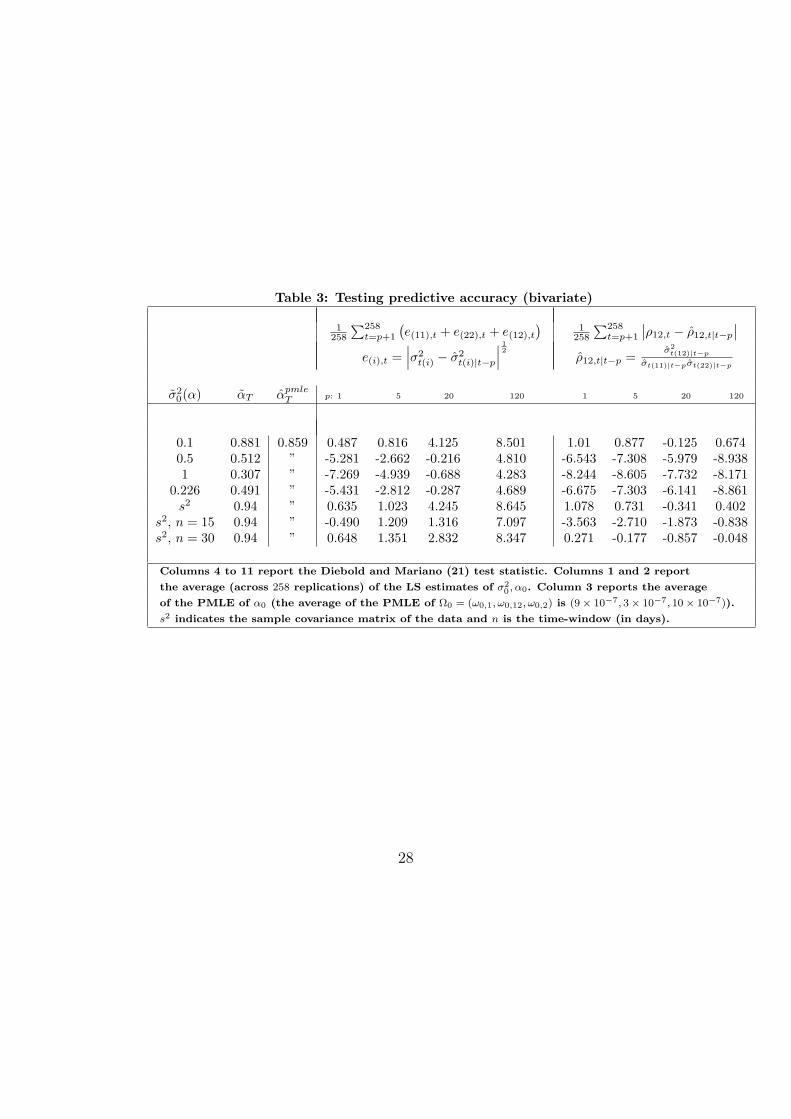
Table 3: Testing predictive accuracy (bivariate)

1258

∑258t=p+1

(e(11),t + e(22),t + e(12),t

)1

258

∑258t=p+1

∣∣ρ12,t − ρ12,t|t−p

∣∣

e(i),t =∣∣∣σ2

t(i) − σ2t(i)|t−p

∣∣∣12

ρ12,t|t−p =σ2

t(12)|t−p

σt(11)|t−pσt(22)|t−p

σ20(α) αT αpmle

T p: 1 5 20 120 1 5 20 120

0.1 0.881 0.859 0.487 0.816 4.125 8.501 1.01 0.877 -0.125 0.6740.5 0.512 ” -5.281 -2.662 -0.216 4.810 -6.543 -7.308 -5.979 -8.9381 0.307 ” -7.269 -4.939 -0.688 4.283 -8.244 -8.605 -7.732 -8.171

0.226 0.491 ” -5.431 -2.812 -0.287 4.689 -6.675 -7.303 -6.141 -8.861s2 0.94 ” 0.635 1.023 4.245 8.645 1.078 0.731 -0.341 0.402

s2, n = 15 0.94 ” -0.490 1.209 1.316 7.097 -3.563 -2.710 -1.873 -0.838s2, n = 30 0.94 ” 0.648 1.351 2.832 8.347 0.271 -0.177 -0.857 -0.048

Columns 4 to 11 report the Diebold and Mariano (21) test statistic. Columns 1 and 2 report

the average (across 258 replications) of the LS estimates of σ20 , α0. Column 3 reports the average

of the PMLE of α0 (the average of the PMLE of Ω0 = (ω0,1, ω0,12, ω0,2) is (9× 10−7, 3× 10−7, 10× 10−7)).

s2 indicates the sample covariance matrix of the data and n is the time-window (in days).

28

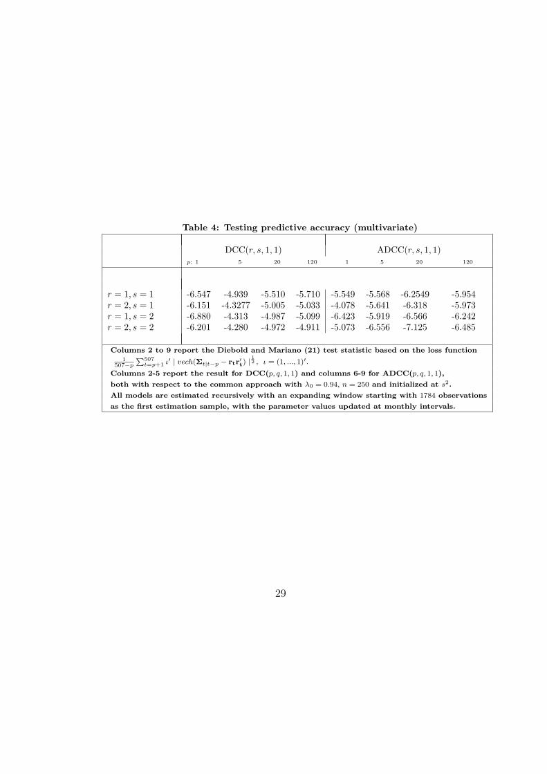
Table 4: Testing predictive accuracy (multivariate)

DCC(r, s, 1, 1) ADCC(r, s, 1, 1)p: 1 5 20 120 1 5 20 120

r = 1, s = 1 -6.547 -4.939 -5.510 -5.710 -5.549 -5.568 -6.2549 -5.954r = 2, s = 1 -6.151 -4.3277 -5.005 -5.033 -4.078 -5.641 -6.318 -5.973r = 1, s = 2 -6.880 -4.313 -4.987 -5.099 -6.423 -5.919 -6.566 -6.242r = 2, s = 2 -6.201 -4.280 -4.972 -4.911 -5.073 -6.556 -7.125 -6.485

Columns 2 to 9 report the Diebold and Mariano (21) test statistic based on the loss function1

507−p

P507t=p+1 ι′ | vech(Σt|t−p − rtr′t) |

12 , ι = (1, ..., 1)′.

Columns 2-5 report the result for DCC(p, q, 1, 1) and columns 6-9 for ADCC(p, q, 1, 1),

both with respect to the common approach with λ0 = 0.94, n = 250 and initialized at s2.

All models are estimated recursively with an expanding window starting with 1784 observations

as the first estimation sample, with the parameter values updated at monthly intervals.

29

Fig

ure

1

-15

-10-505101520

020

0040

0060

0080

0010

000

1200

014

000

-500

-400

-300

-200

-1000

100

200

300

400

500

020

0040

0060

0080

0010

000

1200

014

000

01234567

020

0040

0060

0080

0010

000

1200

014

000

Not

e:Sim

ula

ted

pat

hof

GA

RC

H(1

,1)

r tw

ith

α0

=0.

95an

dω

0=

0(fi

rst

pan

el)

and

ω0

=1

(sec

ond

pan

el)

*an

dof

tr(Σ

t)(c

f.(3

4))

wit

hΩ

0=

0an

dα

0=

0.95

(thir

dpan

el).

Fig

ure

2

0

20

0 0.0

00

.10

0.2

00.3

00

.40

0.5

00.6

00.7

00

.80

0.9

0

IUHTXHQF\

T=

1.0

00

T=

5.0

00

T=

15

.00

0

0

10

20

30

40

50

60

70

80

90

10

0 0.0

00

.10

0.2

00.3

00

.40

0.5

00.6

00.7

00

.80

0.9

01.0

0

IUHTXHQF\

T=

15

.00

0

T=

5.0

00

T=

1.0

00

0

50

10

0 0.9

00

.91

0.9

20.9

30

.94

0.9

50.9

60.9

70

.98

0.9

91.0

0

IUHTXHQF\

T=

15

.000

T=

5.0

00

T=

1.0

00

0

10

0

20

0

30

0

40

0

50

0

60

0 0.0

00

.02

0.0

40

.06

0.0

80

.10

0.1

20

.14

IUHTXHQF\

T=

15

.00

0

T=

5.0

00

T=

1.0

00

0

10

0

20

0

30

0

40

0

50

0

60

0 0.6

50

.67

0.6

90.7

10

.73

0.7

50.7

70.7

90

.81

0.8

3

IUHTXHQF\

T=

15

.00

0

T=

5.0

00

T=

1.0

00

0

50

10

0

15

0

20

0

25

0

30

0

35

0

40

0 0.9

00

.91

0.9

20.9

30

.94

0.9

50.9

60.9

70

.98

0.9

9

IUHTXHQF\

T=

15

.00

0

T=

5.0

00

T=

1.0

00

Not

e:M

onte

carl

odis

trib

uti

on(1

,000

replica

tion

s)of

the

LS

esti

mat

orα

lse

Tw

ith

true

valu

esω

0=

0an

dα

0=

0.05

(firs

tpan

el),

α0

=0.

75*

(sec

ond

pan

el),

α0

=0.

95(t

hir

dpan

el)

and

ofof

the

PM

Les

tim

ator

αpm

leT

wit

htr

ue

valu

esω

0=

1an

dα

0=

0.05

(fou

rth

pan

el),

α0

=0.

75*

(fift

hpan

el),

α0

=0.

95(s

ixth

pan

el).

Est

imat

ion

star

tsfr

oman

init

ialva

lue

ofα

=0.

5.T

he

dot

ted

line

refe

rsto

sam

ple

sof

T=

1,00

0*

obse

rvat

ions,

the

grey

line

tosa

mple

sof

T=

5,00

0ob

serv

atio

ns

and

the

bla

ckline

tosa

mple

sof

T=

15,0

00ob

serv

atio

ns.