DYNAMIC COMPILER OPTIMIZATION TECHNIQUES FORMATLAB
by
Nurudeen Abiodun Lameed
School of Computer Science
McGill University, Montreal
April 2013
A THESIS SUBMITTED TOMCGILL UNIVERSITY
IN PARTIAL FULFILLMENT OF THE REQUIREMENTS OF THE DEGREE OF
DOCTOR OFPHILOSOPHY
Copyright © 2013 by Nurudeen Abiodun Lameed


Abstract
MATLAB has gained widespread acceptance among engineers and scientists. Several
aspects of the language such as dynamic loading and typing, safe updates, copy semantics
for arrays, and support for higher-order functions contribute to its appeal, but at the same
time provide many challenges to the compiler and virtual machine. MATLAB is a dynamic
language. Traditional implementations of the language useinterpreters and have been found
to be too slow for large computations. More recently, researchers and software developers
have been developing JIT compilers for MATLAB and other dynamic languages. This the-
sis is about the development of new compiler analyses and transformations for a MATLAB
JIT compiler, McJIT, which is based on the LLVM JIT compiler toolkit.
The new contributions include a collection of novel analyses for optimizing copying
of arrays, which are performed when a function is first compiled. We designed and imple-
mented four analyses to support an efficient implementationof array copy semantics in a
MATLAB JIT compiler. Experimental results show that copy optimization is essential for
performance improvement in a compiler for the MATLAB language.
We also developed a variety of new dynamic analyses and code transformations for
optimizing running code on-the-fly according to the currentconditions of the runtime en-
vironment. LLVM does not currently support on-the-fly code transformation. So, we first
developed a new on-stack replacement approach for LLVM. This capability allows the run-
time stack to be modified during the execution of a function, thus enabling a continuation
of the execution at a higher optimization level. We then usedthe on-stack replacement
implementation to support selective inlining of function calls in long-running loops. Our
experimental results show that function calls in long-running loops can result in high run-
time overhead, and that selective dynamic inlining can be used to drastically reduce this
i

overhead.
The built-in functionfeval is an important MATLAB feature for certain classes of
numerical programs and solvers which benefit from having functions as parameters. Pro-
grammers may pass a function name or function handle to the solver and then the solver
usesfeval to indirectly call the function. In this thesis, we show thatalthoughfeval
provides an acceptable abstraction mechanism for these types of applications, there are
significant performance overheads for function calls viafeval , in both MATLAB inter-
preters and JITs. The thesis then proposes, implements and compares two on-the-fly mech-
anisms for specialization offeval calls. The first approach uses our on-stack replacement
technology. The second approach specializes calls of functions withfeval using a combi-
nation of runtime input argument types and values. Experimental results on seven numerical
solvers show that the techniques provide good performance improvements.
The implementation of all the analyses and code transformations presented in this thesis
has been done within the McLab virtual machine, McVM, and is available to the public as
open source software.
ii

Resum e
MATLAB est devenu reconnu parmi les ingenieurs et les scientifiques. Plusieurs as-pects du langage comme le chargement et le typage dynamique,la mise a jour sur, lasemantique de copie pour les tableaux, et le support des fonctions d’ordre superieur con-tribuenta son attrait, mais induisent de nombreuses difficultes pour les compilateurs et lesmachines virtuelles. MATLAB est un langage dynamique. Les implementations classiquesdu langage fonctionnent gracea des interpreteurs et sont generalement trop lentes pour deslarges calculs. Plus recemment, les chercheurs ainsi que les programmeurs ont developpedes compilateurs JIT pour MATLAB et d’autres langages dynamiques. Cette these traitele developpement de nouvelles analyses et transformations pour un compilateur JIT MAT-LAB, McJIT, qui est base sur l’outil LLVM.
Ces nouvelles contributions comprennent plusieurs analyses novatrices pour optimiserla copie de tableaux, qui sont executees quand une fonction est compilee pour la premierefois. Nous avons implemente quatre analyses pour permettre une implementation efficacede la semantique de copie de tableaux dans un compilateur JIT MATLAB. Les resultatsexperimentaux montrent que l’optimisation de la copie est essentielle pour ameliorer lesperformances dans un compilateur pour le langage MATLAB.
Nous avons aussi developpe une variete d’analyses dynamiques novatrices et des trans-formations de code pour optimiser du codea la volee en fonction de l’environnementd’execution. Actuellement, LLVM ne supporte pas les transformations de codea la volee.En consequence, nous avons d’abord developpe une nouvelle approche pour faire du rem-placement sur la pile avec LLVM. Cette fonctionnalite permeta la pile d’execution d’etremodifiee pendant l’execution de la fonction, ce qui permet de continuer l’executiona unniveau superieur d’optimisation. Nous avons ensuite utilise cette implementation du rem-placement sur la pile pour permettre l’en line des appels de fonctions dans les boucles. Nosresultats experimentaux montrent que les appels de fonctions dans les bouclesa long tempsd’execution peuvent induire un cout important en termes de performances, et que l’en line
iii

dynamique et selectif peutetre utilise pour reduire drastiquement ce cout.La fonction ”feval” est une fonctionnalite importante de MATLAB pour certains pro-
grammes de calcul numerique qui profitent de la possibilite de passer des fonctions commeparametres. Les programmeurs peuvent passer le nom d’une fonction ou un pointeur defonctionsa un programme qui utilisera ensuite feval pour appeler indirectement cette fonc-tion. Dans cette these, nous montrons que malgre le fait que feval soit un mecanismed’abstraction appreciable pour certaines applications, il induit un cout significatif, a lafois pour les interpreteurs et pour les compilateurs JIT. Cette these propose, implementeet compare deux mecanismesa la volee pour la specialisation des appels utilisant feval.La premiere methode utilise notre mecanisme de remplacement sur la pile. La secondemethode specialise les appels de fonctions utilisant feval en combinant le type et la valeurdes argumentsa l’execution. Les resultats experimentaux sur sept programmes differentsmontrent que ces techniques permettent une bonne amelioration des performances.
L’impl ementation de toute les analyses et transformations de codepresentees dans cette
these aete effectue dans la machine virtuelle McLab, appelee McVM, et est disponible au
public en tant que logiciel libre.
iv

Acknowledgements
First, I would like to thank my supervisor, Professor LaurieHendren, for her support
and constant encouragement. I benefited greatly from her intelligence and wealth of expe-
rience. Her insightful comments and suggestions helped a lot to improve this thesis.
I thank Professor Clark Verbrugge and all the members of my PhDcommittee for their
useful comments and suggestions on both the proposal and thefinal version of this thesis. I
also thank Professor Jose Nelson Amaral for his suggestionsfor improving the final version
of the thesis.
I thank all the members of the Sable Group, in particular, themembers of the McLAB
team for their contributions to the McLAB project. I would like to thank Maxime Chevalier-
Boisvert for developing the first version of McVM.
I am grateful to Matthieu Dubet and Kamal Zellag for their help in translating the
abstract of this thesis into French language.
I wish to thank the School of Computer Science Systems staff and the administrative
staff for their support in my role as the system administrator for Sable Lab.
Many friends have helped me throughout my programme at McGill. I thank you all.
I am grateful to FQRNT for their financial support. This thesiswas partly supported by
NSERC as well.
Finally, I would like to thank my family, my beloved wife, Aderonke and my children,
Hanifah, Azizah and Ibrahim, for their support, encouragement and understanding without
which this thesis would have been impossible to undertake.
v

vi

Contents
Abstract i
Resume iii
Acknowledgements v
Contents vii
Contents xiii
List of Figures xv
List of Tables xvii
List of Abbreviations xix
1 Introduction 1
1.1 Virtual Machines . . . . . . . . . . . . . . . . . . . . . . . . . . . . . . . 2
1.1.1 JIT Compilation . . . . . . . . . . . . . . . . . . . . . . . . . . . 3
1.2 Motivation . . . . . . . . . . . . . . . . . . . . . . . . . . . . . . . . . . . 4
1.2.1 Characteristics of MATLAB Programs . . . . . . . . . . . . . . . .5
1.3 Challenges . . . . . . . . . . . . . . . . . . . . . . . . . . . . . . . . . . . 5
1.3.1 Challenge 1: Copy Semantics . . . . . . . . . . . . . . . . . . . . 6
1.3.2 Challenge 2: Function Calls in Loops . . . . . . . . . . . . . . . . 7
1.3.3 Challenge 3: Dynamic Function Evaluation (feval) . . . . . . . . . 8
vii

1.4 Solution Overview . . . . . . . . . . . . . . . . . . . . . . . . . . . . . . 9
1.4.1 Copy Optimization . . . . . . . . . . . . . . . . . . . . . . . . . . 10
1.4.2 On-Stack-Replacement (OSR) Support . . . . . . . . . . . . . . . 10
1.4.3 Selective Dynamic Inlining of Function Calls in Loops .. . . . . . 11
1.4.4 feval Call Specialization . . . . . . . . . . . . . . . . . . . . . . 11
1.5 Research Contributions . . . . . . . . . . . . . . . . . . . . . . . . . . . . 11
1.5.1 Copy Optimization in McVM . . . . . . . . . . . . . . . . . . . . 12
1.5.2 Modular On-Stack Replacement in LLVM . . . . . . . . . . . . . . 12
1.5.3 Selective Dynamic Inlining . . . . . . . . . . . . . . . . . . . . . .12
1.5.4 Dynamic Function Dispatch via the MATLABfeval . . . . . . . 13
1.6 The Organization of the Thesis . . . . . . . . . . . . . . . . . . . . . .. . 13
2 Background: MATLAB, McVM and LLVM Compiler Framework 15
2.1 MATLAB . . . . . . . . . . . . . . . . . . . . . . . . . . . . . . . . . . . 15
2.2 The McLab Virtual Machine . . . . . . . . . . . . . . . . . . . . . . . . . 18
2.2.1 Type Inference and Specialization . . . . . . . . . . . . . . . .. . 21
2.2.2 Running a Function . . . . . . . . . . . . . . . . . . . . . . . . . . 21
2.2.3 McJIT-Interpreter Interaction . . . . . . . . . . . . . . . . . .. . 22
2.3 The LLVM Compiler Framework . . . . . . . . . . . . . . . . . . . . . . . 23
2.3.1 The Three-Phase Design of LLVM . . . . . . . . . . . . . . . . . . 23
2.3.2 Static Single Assignment (SSA) Form . . . . . . . . . . . . . . .. 25
2.3.3 LLVM IR: Examples . . . . . . . . . . . . . . . . . . . . . . . . . 28
2.3.4 LLVM Transformation and Optimization Pass . . . . . . . . .. . . 30
2.3.5 LLVM JIT Execution Engine . . . . . . . . . . . . . . . . . . . . . 32
2.4 Summary . . . . . . . . . . . . . . . . . . . . . . . . . . . . . . . . . . . 33
3 Copy Optimization in MATLAB 35
3.1 Background . . . . . . . . . . . . . . . . . . . . . . . . . . . . . . . . . . 37
3.2 Quick Check . . . . . . . . . . . . . . . . . . . . . . . . . . . . . . . . . 38
3.3 Necessary Copy Analysis . . . . . . . . . . . . . . . . . . . . . . . . . . . 40
3.3.1 Domain . . . . . . . . . . . . . . . . . . . . . . . . . . . . . . . . 40
viii

3.3.2 Problem Definition . . . . . . . . . . . . . . . . . . . . . . . . . . 40
3.3.3 Flow Function . . . . . . . . . . . . . . . . . . . . . . . . . . . . 41
3.3.4 Initialization . . . . . . . . . . . . . . . . . . . . . . . . . . . . . 43
3.3.5 Simple Example . . . . . . . . . . . . . . . . . . . . . . . . . . . 44
3.3.6 if-else Statement . . . . . . . . . . . . . . . . . . . . . . . . . . . 45
3.3.7 Loops . . . . . . . . . . . . . . . . . . . . . . . . . . . . . . . . . 45
3.4 Copy Placement Analysis . . . . . . . . . . . . . . . . . . . . . . . . . . . 45
3.4.1 Abstraction . . . . . . . . . . . . . . . . . . . . . . . . . . . . . . 46
3.4.2 Statement Sequence . . . . . . . . . . . . . . . . . . . . . . . . . 47
3.4.3 if -else Statements . . . . . . . . . . . . . . . . . . . . . . . . . . 48
3.4.4 Loops . . . . . . . . . . . . . . . . . . . . . . . . . . . . . . . . . 49
3.5 Using the Analyses . . . . . . . . . . . . . . . . . . . . . . . . . . . . . . 49
3.6 Name Resolution . . . . . . . . . . . . . . . . . . . . . . . . . . . . . . . 54
3.7 Experimental Results . . . . . . . . . . . . . . . . . . . . . . . . . . . . . 55
3.7.1 Dynamic Counts of Array Updates and Copies . . . . . . . . . . . 56
3.7.2 The Overhead of Dynamic Checks . . . . . . . . . . . . . . . . . 58
3.7.3 Impact of our Analyses . . . . . . . . . . . . . . . . . . . . . . . 60
3.8 Summary . . . . . . . . . . . . . . . . . . . . . . . . . . . . . . . . . . . 62
4 A Modular Approach to On-Stack Replacement in LLVM 63
4.1 OSR Classification . . . . . . . . . . . . . . . . . . . . . . . . . . . . . . 65
4.2 The OSR API . . . . . . . . . . . . . . . . . . . . . . . . . . . . . . . . . 67
4.2.1 Adding the OSR Point Inserter . . . . . . . . . . . . . . . . . . . . 68
4.2.2 Adding the OSR Transformation Pass . . . . . . . . . . . . . . . .71
4.2.3 Initialization and Finalization . . . . . . . . . . . . . . . . .. . . 72
4.3 Implementation . . . . . . . . . . . . . . . . . . . . . . . . . . . . . . . . 73
4.3.1 Implementation Challenges . . . . . . . . . . . . . . . . . . . . . 73
4.3.2 OSR Point . . . . . . . . . . . . . . . . . . . . . . . . . . . . . . 74
4.3.3 The OSR Pass . . . . . . . . . . . . . . . . . . . . . . . . . . . . 74
4.3.3.1 Saving Live Values . . . . . . . . . . . . . . . . . . . . 77
4.3.4 Restoration of State and Recompilation . . . . . . . . . . . . . .. 78
ix

4.3.4.1 Restoration of State . . . . . . . . . . . . . . . . . . . . 80
4.3.4.2 Recompilation . . . . . . . . . . . . . . . . . . . . . . . 83
4.3.5 Inlining Support . . . . . . . . . . . . . . . . . . . . . . . . . . . 84
4.4 Summary . . . . . . . . . . . . . . . . . . . . . . . . . . . . . . . . . . . 85
5 Selective Dynamic Inlining in McVM 87
5.1 The McJIT dynamic inliner . . . . . . . . . . . . . . . . . . . . . . . . . .88
5.2 Symbol Environment Simplification . . . . . . . . . . . . . . . . . .. . . 90
5.3 Experimental Results . . . . . . . . . . . . . . . . . . . . . . . . . . . . . 94
5.3.1 Cost of Code Instrumentation and OSR . . . . . . . . . . . . . . . 99
5.3.2 Effectiveness of Selective Inlining With OSR . . . . . . .. . . . . 100
5.4 Summary . . . . . . . . . . . . . . . . . . . . . . . . . . . . . . . . . . . 102
6 Dynamic Function Evaluation with feval 103
6.1 Motivation and Problem . . . . . . . . . . . . . . . . . . . . . . . . . . . 104
6.2 Summary . . . . . . . . . . . . . . . . . . . . . . . . . . . . . . . . . . . 111
7 OSR-Basedfeval Specialization 113
7.1 feval in McVM . . . . . . . . . . . . . . . . . . . . . . . . . . . . . . . 114
7.1.1 OSR Background . . . . . . . . . . . . . . . . . . . . . . . . . . . 115
7.2 OSR-Basedfeval Transformation . . . . . . . . . . . . . . . . . . . . . 115
7.2.1 feval Optimization Goals and Strategy . . . . . . . . . . . . . . 116
7.2.2 Dispatcher Call Site Annotation . . . . . . . . . . . . . . . . . . .117
7.2.3 OSR Instrumentation . . . . . . . . . . . . . . . . . . . . . . . . . 118
7.2.4 OSR Triggering and Runtime Transformation . . . . . . . . . .. . 119
7.2.5 Runtime Guards . . . . . . . . . . . . . . . . . . . . . . . . . . . 123
7.2.6 Resuming Execution after an OSR is Triggered . . . . . . . . .. . 126
7.3 Experimental Results . . . . . . . . . . . . . . . . . . . . . . . . . . . . . 126
7.4 Summary . . . . . . . . . . . . . . . . . . . . . . . . . . . . . . . . . . . 129
8 JIT Value-Based Specialization 131
8.1 JIT Code Specialization . . . . . . . . . . . . . . . . . . . . . . . . . . . .132
x

8.1.1 Functions of the Dispatcher . . . . . . . . . . . . . . . . . . . . . 134
8.1.2 General Dispatcher . . . . . . . . . . . . . . . . . . . . . . . . . . 136
8.2 Experimental Results . . . . . . . . . . . . . . . . . . . . . . . . . . . . . 138
8.2.1 JIT value-based-specialization approach . . . . . . . . .. . . . . . 138
8.2.2 A comparison of the OSR-based and JIT value-based-
specialization approaches . . . . . . . . . . . . . . . . . . . . . . . 139
8.3 Summary . . . . . . . . . . . . . . . . . . . . . . . . . . . . . . . . . . . 141
9 Related Work 143
9.1 Copy Optimization . . . . . . . . . . . . . . . . . . . . . . . . . . . . . . 143
9.2 On-Stack Replacement . . . . . . . . . . . . . . . . . . . . . . . . . . . . 145
9.3 Selective Dynamic Inlining . . . . . . . . . . . . . . . . . . . . . . . .. . 146
9.4 OSR-Basedfeval Specialization . . . . . . . . . . . . . . . . . . . . . . 147
9.5 JIT Value-Based Specialization . . . . . . . . . . . . . . . . . . . . .. . . 149
10 Conclusions and Future Work 151
10.1 Future Work . . . . . . . . . . . . . . . . . . . . . . . . . . . . . . . . . . 153
A Relevant McVM compilation flags 167
B Copy optimization aspect 169
xi

xii

Listings
1.1 A while loop with anfeval call. . . . . . . . . . . . . . . . . . . . . . . 9
2.1 A matrix multiplication MATLAB function. . . . . . . . . . . . .. . . . . 16
2.2 A matrix multiplication driver. . . . . . . . . . . . . . . . . . . . .. . . . 17
2.3 A matrix multiplication driver using MATLAB “*” operator. . . . . . . . . 17
2.4 A MATLAB function with anif-elsestatement. . . . . . . . . . . . . . . . 26
2.5 A simple MATLAB function. . . . . . . . . . . . . . . . . . . . . . . . . . 28
2.6 LLVM IR for addDoubles. . . . . . . . . . . . . . . . . . . . . . . . . . . 28
2.7 A naive implementation oftest (Listing 2.4) in LLVM IR. . . . . . . . . . 29
2.8 A more optimized implementation oftest(Listing 2.4) in LLVM IR. . . . . 30
2.9 An example of a function pass. . . . . . . . . . . . . . . . . . . . . . . .. 31
2.10 Creating a JIT execution engine. . . . . . . . . . . . . . . . . . . . .. . . 33
3.1 A MATLAB function (tridisolve). . . . . . . . . . . . . . . . . . . . . . . 52
4.1 A code transformer. . . . . . . . . . . . . . . . . . . . . . . . . . . . . . . 70
4.2 Sample code for inserting an OSR point. . . . . . . . . . . . . . . .. . . . 71
4.3 The OSR Pass interface. . . . . . . . . . . . . . . . . . . . . . . . . . . . 72
4.4 Initialization and Finalization in the JIT’smainfunction. . . . . . . . . . . 72
4.5 OSR instrumentation. . . . . . . . . . . . . . . . . . . . . . . . . . . . . .78
5.1 The inner loop ofsim anl. . . . . . . . . . . . . . . . . . . . . . . . . . . 91
5.2 LLVM code forsim anl entry basic block. (We show only the most rele-
vant instructions.) . . . . . . . . . . . . . . . . . . . . . . . . . . . . . . . 92
5.3 Functionmu inv. . . . . . . . . . . . . . . . . . . . . . . . . . . . . . . . 92
5.4 McJIT generated LLVM code formu inv. . . . . . . . . . . . . . . . . . . 93
xiii

6.1 Newton’s method to find a root of the scalar equation f(x) =0, adapted
from [Rec00a,Rec00b]. Functionfx3n is shown in Listing 6.2. . . . . . . . 105
6.2 Functionfx3nfrom [Rec00a,Rec00b]. . . . . . . . . . . . . . . . . . . . . 105
7.1 LLVM code generated for anfeval call. . . . . . . . . . . . . . . . . . . 114
7.2 while loop extracted from (Listing 6.1). . . . . . . . . . . . . . . . . . . . 119
8.1 TheodeRK4benchmark (from [Rec00a,Rec00b]). . . . . . . . . . . . . . 140
xiv

List of Figures
2.1 Overview of the McLAB project (shaded boxes are contributions of this
thesis). . . . . . . . . . . . . . . . . . . . . . . . . . . . . . . . . . . . . . 19
2.2 The main components of McVM (adapted from [CB09]). The shaded com-
ponents are parts of the research work presented in this thesis. . . . . . . . 20
2.3 Running a function in McVM. . . . . . . . . . . . . . . . . . . . . . . . . 22
2.4 Three-phase Design of LLVM (adapted fromThe Architecture of Open
Source[BW11]). To implement the MATLAB language in LLVM, a MAT-
LAB front-end must be implemented. . . . . . . . . . . . . . . . . . . . . 24
2.5 A CFG for functiontest is shown in (a); an equivalent CFG for the function
in SSA form is shown in (b). . . . . . . . . . . . . . . . . . . . . . . . . . 26
3.1 A simplified overview of McJIT (shaded boxes correspond to the analyses
presented in this chapter). . . . . . . . . . . . . . . . . . . . . . . . . . . .37
3.2 The total bytes of array data copied by the benchmarks under the three
options. . . . . . . . . . . . . . . . . . . . . . . . . . . . . . . . . . . . . 60
4.1 OSR classification. . . . . . . . . . . . . . . . . . . . . . . . . . . . . . . 66
4.2 Retrofitting an existing JIT with OSR support. . . . . . . . . . .. . . . . . 68
4.3 A CFG of a loop with no OSR points. . . . . . . . . . . . . . . . . . . . . 75
4.4 The CFG of the loop in Figure 4.3 after inserting an OSR point. . . . . . . 76
4.5 The transformed CFG of the loop in Figure 4.4 after runningthe OSR Pass. 77
4.6 State management cycle. . . . . . . . . . . . . . . . . . . . . . . . . . . .79
4.7 A CFG of a loop of a running function before inserting the blocks for state
recovery. . . . . . . . . . . . . . . . . . . . . . . . . . . . . . . . . . . . . 81
xv

4.8 The CFG of the loop represented by Figure 4.7 after inserting the state
recovery blocks. . . . . . . . . . . . . . . . . . . . . . . . . . . . . . . . . 82
5.1 A loop nest showing the placement of OSR points using the closest or
outer-most strategy. . . . . . . . . . . . . . . . . . . . . . . . . . . . . . . 89
7.1 A CFG for the MATLABwhile loop in Figure 7.2. . . . . . . . . . . . . . 119
7.2 The CFG of a loop with an OSR point. . . . . . . . . . . . . . . . . . . . . 120
7.3 Actions of the code transformer. Basic blockOBB in (a) is split into two.
The result of the splitting process is shown in (b). In (c),NBB is split
into NBB andCONTBB. A new unlinked basic block namedCBB is also
generated.CBBcontains a call to the new compiled function (f ). . . . . . . 121
7.4 Actions of the code Transformer. Two new basic blocks have been inserted
into the CFG:CBBcontains a call to the compiled function (f ), andMBB
merges the results from the call inCBB and the original call to the dis-
patcher inNBB. . . . . . . . . . . . . . . . . . . . . . . . . . . . . . . . . 121
8.1 feval Runtime Code Specialization. . . . . . . . . . . . . . . . . . . . . 132
xvi

List of Tables
1.1 Some characteristics of MATLAB programs . . . . . . . . . . . . .. . . . 5
3.1 Forward Analysis result forexample1. . . . . . . . . . . . . . . . . . . . . 45
3.2 Necessary Copy and Copy Placement Analyses fortest3. . . . . . . . . . . 50
3.3 Necessary Copy Analysis Result. . . . . . . . . . . . . . . . . . . . . . .. 53
3.4 Copy Placement Analysis Result fortridisolve. . . . . . . . . . . . . . . . 54
3.5 . . . . . . . . . . . . . . . . . . . . . . . . . . . . . . . . . . . . . . . . 57
3.6 Overhead of Dynamic Checks. . . . . . . . . . . . . . . . . . . . . . . . . 59
3.7 Benchmarks against the total execution times in seconds.. . . . . . . . . . 61
5.1 The benchmarks. . . . . . . . . . . . . . . . . . . . . . . . . . . . . . . . 95
5.2 OSR Overhead. . . . . . . . . . . . . . . . . . . . . . . . . . . . . . . . . 97
5.3 Dynamic inlining using OSR (lower execution ratio is better). . . . . . . . 98
6.1 feval benchmarks. . . . . . . . . . . . . . . . . . . . . . . . . . . . . . 107
6.2 Interpreter:feval overheads as compared to direct and inlined calls. . . . 109
6.3 JIT:feval overheads as compared to direct and inlined calls. . . . . . . . 110
7.1 Guard truth table (a “*” denotes an impossible result). .. . . . . . . . . . . 125
7.2 Overall results for OSR-based optimitimzation in McVM JIT . . . . . . . . 127
7.3 Types of the runtime guards used by each benchmark. . . . . .. . . . . . . 128
8.1 Comparing Value-based specialization to OSR-based and hand-coded . . . 139
xvii

xviii

List of Abbreviations
AST abstract syntax tree
CFG control flow graph
IR intermediate representation
JIT just-in-time
JVM Java virtual machine
OSR on-stack replacement
RC reference-counting
SSA static single assignment
VM virtual machine
xix

xx

Chapter 1
Introduction
Almost anyone using a computing device today has used a program written in a dy-
namic language. A large proportion of Internet applications are developed with dynamic
languages. JavaScript, Perl, PHP, Python, Ruby, and MATLAB ® 1 are some of the widely
used dynamic languages. They shared a common property: theyare dynamically typed.
Their dynamic nature contributes to their appeal. But it alsocontributes to their compila-
tion difficulty. Thus, they are mostly interpreted, and programs written in any of them often
run slower than those written in a static language such as C.
The MATLAB programming language is a dynamic array-based language that is pop-
ular among engineers and scientists. It was designed for sophisticated matrix and vector
operations, which are common in scientific applications. The MATLAB programming lan-
guage is an important language with a simple syntax. It is being used in different computing
domains. By the year 2004, the number of MATLAB users had exceeded one million. Fur-
ther, much like the way transistor growth in microprocessordesign has obeyed the famous
Moore’s law [Moo65], the number of users of the MATLAB language doubled about every
two years between 1984 and 2004, and continues to increase.
The dynamic nature of the MATLAB language, together with itssimple syntax, aids
rapid software development by helping programmers to reason about their programs. The
combination, however, poses serious compilation and performance challenges. Dynamic
1. http://www.mathworks.com/products/pfo/.
1

Introduction
language features such as dynamic function loading causes the compiler to delay most
optimizations until run time. This increases runtime overhead.
Traditional implementations of the MATLAB programming language are based on in-
terpreters [gnu12, The02]. They are generally considered to be too slow for long-running
MATLAB programs. Recently, researchers and developers havebeen developing virtual
machines and just-in-time compilers [AP02,The02,CB09,CBHV10] for the MATLAB lan-
guage. There remain, however, important compilation challenges. Although the dynamic
nature of the MATLAB language provides challenges to runtime optimizations, it also
presents great opportunities. For example, the runtime behaviour of a MATLAB program
can be observed to discover opportunities for optimizationand an on-the-fly optimizer can
dynamically apply suitable optimizations that benefit fromthe identified opportunities.
This thesis is about the development of a collection of noveltechniques for on-the-fly
transformations and optimizations in JIT compilers for theMATLAB language. We show
how to use runtime information about program behaviour to support transformations and
optimizations that can improve the performance of virtual machines and JIT compilers for
the MATLAB programming language.
We begin this chapter of the thesis with an introduction to virtual machines and JIT
compilers. Later, we briefly review a study that further motivates our research work. We
then highlight the challenges and our solutions that address the challenges. Further, we
summarize our main research contributions. We conclude thechapter with the organization
of the remaining chapters of the thesis.
1.1 Virtual Machines
The increasing growth of the Internet is driving a growing interest in virtualization
among hardware designers, operating system designers, programming language design-
ers, and compiler writers. In many systems, virtualizationhas helped to achieve cross-
platform independence, inter-operability (i.e., high-level language independence), security,
and cross-platform performance. In the past, the main motivation for building virtual ma-
chines was to run different operating systems on shared hardware. This was necessary to
2

1.1. Virtual Machines
support different computational needs of different group of users on shared hardware.
Virtual machines provided a transformation of the single interface of a computer sys-
tem into manyvirtual interfaces [Gol73, PG74]. Each interface behaves like a complete
computer system that is composed of an operating system and support many simultaneous
user processes. Hence, they are calledsystemvirtual machines [SN05].
A processvirtual machine supports only a single process. Virtual machines for high-
level languages (e.g., McVM, JVM [LY99], and CLR [Int13]) areprocess virtual machines.
They are typically designed to provide platform independence by reconciling differences
in architectures and operating systems. In this thesis, we are concerned only with imple-
mentations of process virtual machines.
A system’s interface is specified by its instruction set architecture (ISA). Virtual ma-
chines are implemented by emulating the instruction set of one system — thesource—
on a machine with a different instruction set — thetarget. A process virtual machine pro-
vides a machine-independent interface that is similar to a conventional machine instruction
set architecture. The ISA of a virtual machine is called virtual instruction set architecture
(V-ISA).
Many V-ISAs have been designed.P-code[NAJ+75] is a V-ISA for the Pascal machine;
similarly, Java byte codesis a V-ISA for the Java virtual machine. Microsoft intermediate
language (MSIL) (or common intermediate language (CLI) for Microsoft’s common lan-
guage infrastructure (CLI)) [Int13] and LLVM [LA04] are moregeneral V-ISAs.
The virtual instruction set of a virtual machine can be interpreted or compiled. This
thesis concentrates on JIT compilation techniques.
1.1.1 JIT Compilation
Compilation concerns the translation of one language into another language. A spe-
cial translation technique used in implementing virtual machines is the JIT (Just-In-Time)
compilation technique. JIT compilation is an old technique. It was developed in response
to the performance challenges of the interpretation techniques used in implementing virtual
machines.
3

Introduction
Instead of interpreting virtual instructions, some blocksof code are now compiled just
before they are executed. Thus repeated execution of the same code requires no further
interpretation or compilation. This approach combines thebenefits of static compilation:
compiled code generally runs faster than interpreted code.It also brings the benefits of in-
terpretation because the compilation process can benefit from semantic and runtime infor-
mation. According to Aycock [Ayc03], McCarthy’s paper on LISP [McC60] is the first pub-
lished work on JIT compilation. Several techniques for JIT compilation of object-oriented
languages were developed in several implementations of Smalltalk [GR83,DS84a,Kay93],
SELF [Cha92], and, more recently, in many implementations ofJava virtual machines
[ATCL+98,YMP+99,Kra98,CLS00,PVC01,SOK+04,AAB+05].
Some virtual machines have interpreters and JIT compilers.Some other VMs begin with
a base-line compiler and recompile methods or functions with a more optimizing compiler
after identifying some frequently executed methods or coderegions — thehot spots. The
optimizing compiler often performs a range of optimizations, including, traditional opti-
mizations such as register allocation, inlining, common sub-expression elimination, and
other runtime optimization tailored to exploit some relevant runtime information.
McVM [CBHV10] is a recent virtual machine developed for the MATLAB language.
It has a basic interpreter and an optimizing JIT compiler that is supported by the LLVM
[LA04] compiler framework. We introduce the MATLAB language, McVM and LLVM in
Chapter 2.
1.2 Motivation
Over the years, numerous MATLAB programs have been developed to solve a variety of
problems in different domains, in particular the numericalcomputing domain. To gain some
insight into the way different MATLAB programmers use the features of the MATLAB
language, a study of MATLAB programs is necessary. This willhelp in the identification
of the important features in MATLAB programs; further, it may also reveal some major
sources of overhead. In this section, we describe a study conducted on a large collection of
MATLAB programs.
4

1.3. Challenges
1.2.1 Characteristics of MATLAB Programs
To discover the common characteristics of MATLAB programs,we conducted a study
of a large collection of MATLAB programs.2 The result of this study is shown in Table 1.1.
Out of 12,946 functions in 3,114 files examined, 31% (3,992) contain loops; 41% (4,356)
of the loops contain conditional statements while 62% (6,681) of the loops have function
calls. About 95% (12,270) of the functions have one or more input parameters while 54%
(6,954) have one or more output parameters.
The results of this study provide a guide to the identification of key optimizations that
address many of the compilation and performance challengesin a MATLAB compiler. we
examine the challenges and opportunities in MATLAB programs in the next section.
Property Count
Number of files 3,114
Number of functions 12,946
Number of functions with input parameters 12,270
Number of functions with output parameters 6,954
Number of functions with both input and output parameters6,664
Number of functions with loops 3,992
Number of loops 10,726
Number of loops with conditionals 4,356
Number of loops with calls 6,681
Table 1.1 – Some characteristics of MATLAB programs
1.3 Challenges
A typical MATLAB program operates on large arrays. Althoughmany of these opera-
tions are difficult to compile efficiently, static and dynamic optimization opportunities exist.
2. These MATLAB programs were collected from a variety of sources, including those from:
http://www.mathworks.com/matlabcentral/fileexchange ,
http://people.sc.fsu.edu/ ˜ jburkardt/m_src/m_src.html ,
http://www.csse.uwa.edu.au/ ˜ pk/Research/MatlabFns/ and
http://www.mathtools.net/MATLAB/.
5

Introduction
In this section, we highlight some performance challenges and optimization opportunities
in MATLAB programs.
1.3.1 Challenge 1: Copy Semantics
The use of copy semantics for array assignments, for parameter passing and for return-
ing values from a function is one of the cases where the simplesemantics of the MAT-
LAB language helps the programmer to reason about the code but provides performance
challenges. Assignment statements in the MATLAB programming language have different
forms, for example:
a = zeros(10); (1.1)
b = a; (1.2)
c = myfunc(a, b); (1.3)
A naive implementation of the copy semantics for statements1.1 - 1.3 above would involve
making a copy at every assignment statement. Thus, in statement 1.1, the object (a 10 x
10 matrix) allocated by functionzeroswould be copied into variablea. The MATLAB
language defines a number of memory allocation functions similar to zeros. In statement
1.2, arraya would be copied into variableb. In statement 1.3, the argumentsa andb in
the call to functionmyfuncwould be copied into their corresponding parameters of the
function; the return value ofmyfuncwould also copied into variablec.
With this naive strategy a copy must be generated when: 1) a variable is defined from
an existing object; 2) a parameter is passed from one function to another; and 3) a value
is returned from a function. Obviously, this is inefficient.A more advanced implementa-
tion can detect opportunities to convert copy-by-value to copy-by-reference, and similarly,
convert call-by-value to call-by-reference.
The results in Table 1.1 shows that most MATLAB functions have one or more input
and/or output parameters. This suggests that in a naive implementation, array copying is
potentially a major generator of runtime overhead.
6

1.3. Challenges
Existing MATLAB systems rely on reference-counting schemes to create copies only
when a shared array representation is updated. This reducesarray copies, but increases the
number of runtime checks.
In addition, reference-counting schemes incur overheads.The approach requires space
for storing a reference count for each array object and spacefor the code that keeps the
reference counts updated. Keeping the reference counts updated also generates execution
time overhead. Hence, adding a reference-counting scheme to a garbage-collected runtime
system will have a negative effect on performance.
Because copying large arrays affects performance, an efficient implementation of ar-
ray copy semantics in MATLAB is a key optimization for improving the performance of
MATLAB programs.
1.3.2 Challenge 2: Function Calls in Loops
The results of the study of MATLAB programs (Table 1.1) reveal that MATLAB pro-
grams often contain loops. This is not surprising because MATLAB is an array-based lan-
guage and loops are typically used to express repetitive operations on arrays. It was also
found that a significant proportion of the loops studied havefunction calls. Based of these
results, we can predict that the called functions in those loops are frequently executed. If
this happens, it will result in excessive function call overheads. Besides, function calls gen-
erally disrupt optimizations, forcing many analyses and transformations to be necessarily
conservative. It is also hard to vectorize a loop that contains function calls.
An important optimization technique for eliminating function call and return overheads
is function inlining or inline expansion. Inlining optimization involves replacing a call in-
struction at a call site with the body of the called function.Inlining of call sites that are
frequently executed can lead to an improved performance. Asan example, consider the
following code snippet.
7

Introduction
1 n = 10000;2 ...3 for i=1:n4 ...5 compute(i) % a potentially hot call6 ...7 end
The call of functioncomputein line 5 can prevent loop optimizations such as vectoriza-
tion. By first inlining compute, however, we increase the opportunity for vectorization and
increase the scope for the traditional compiler optimizations. Also, ifcomputeis a straight-
line code, the loop computation can be performed on a GPU. Thechallenge therefore is to
dynamically identify and inline the most critical call sites that can lead to a performance
improvement.
1.3.3 Challenge 3: Dynamic Function Evaluation ( feval)
The problem with the dynamic function evaluation viafeval is related to Challenge 2.
An important feature of the MATLAB programming language is its support of higher-order
functions through thefeval construct, which is widely used in many classes of numeri-
cal computations, including fitting functions, estimatingOrdinary Differential Equations
(ODE), machine learning algorithms such as simulated annealing, and general plotting
functions. All of these applications share a similar pattern, the main computation func-
tion has a function parameter that can accept either a function handle, or a function name
as the actual argument. The body of the computation functionthen repeatedly evaluates the
function passed in usingfeval .
However, dynamic function evaluation viafeval calls within a frequently executed
loop can incur high runtime overhead. Thefeval call is often interpreted because the
function to be evaluated is generally unknown at the compilation time. This can be very
slow. Besides, function evaluation viafeval built-in prevents important optimizations
such as inlining that can increase the scope for other more traditional compiler optimiza-
tions such as the common sub-expression elimination (CSE). The challenge therefore is
to determine the overhead offeval and to develop runtime optimization techniques for
reducing or eliminating the overhead, and thus improve performance.
8

1.4. Solution Overview
Listing 1.1 – A while loop with anfeval call.1 while k ≤ maxit2 k = k + 1;3 [ f ,dfdx] = feval (fun,x ); %Returns f( x(k−1) ) and f '( x(k−1) )4 dx = f /dfdx;5 x = x − dx;6 if ( ( abs(f ) < feps ) | ( abs(dx) < xeps ) )7 r = x;8 return ;9 end
10 end11 end
Listing 1.1 shows a MATLAB code snippet from Gerald Recktenwald’s [Rec00a] im-
plementation of Newton’s method for finding the root of a polynomial. The code snippet
contains a loop with anfeval call. The first argument to thefeval call, that is,fun
contains the name or a handle to the function that thefeval call evaluates at run time.
An optimization opportunity exists: becausefun is a loop constant, then thefeval call
will evaluate the same function at every iteration of the loop. Replacing thefeval call
with a direct call to the function held by variablefun can lead to a significant performance
improvement.
In the next section, we provide an overview of the techniquesthat we have developed
to overcome these challenges. We describe the techniques indetail in chapters 3 — 8.
1.4 Solution Overview
The foregoing challenges have been resolved in this thesis by developing suitable opti-
mization techniques as an extension to McJIT, the McVM JIT compiler [CB09,CBHV10].
Three major optimization opportunities that have been identified and addressed are:
1. array copying at assignments and input or output parameter passing;
2. a high number of loops, and a high proportion of loops with function calls;
3. repeated evaluation of a fixed target function by anfeval call.
9

Introduction
1.4.1 Copy Optimization
To harness the first optimization opportunity, we developedan approach that is based
on JIT-time static flow analysis. It is a staged static analysis approach that does not require
reference counts, thus enabling a garbage-collected virtual machine. It eliminates both un-
needed array copies and does not require frequent runtime checks.
The first stage combines two simple, yet fast, intraprocedural forward analyses to elim-
inate unnecessary copies: the first,written parametersanalysis determines the parameters
thatmaybe modified by a function while the second,copy replacementanalysis determines
if all the uses of a copy variable can be replaced by the original so that the copy statement
defining the copy can be eliminated.
The second stage is comprised of two analyses that together determine whether a copy
should be performed before an array is updated: the first,necessary copy analysis, is a
forward flow analysis and determines the program points where array copies are required
while the second,copy placement analysis, is a backward analysis that finds the optimal
points to place copies, which also guarantee safe array updates. We return to copy opti-
mization analyses in Chapter 3.
1.4.2 On-Stack-Replacement (OSR) Support
To ensure that a function that is in the middle of an executioncan be optimized at a
higher optimization level, the dynamic optimizations highlighted below must be supported
by an on-stack replacement capability. Unfortunately, however, LLVM does not support
on-stack replacement.
So, we implemented OSR for LLVM. We decided to design and develop a modular
approach to implementing on-stack replacement in LLVM as part of the research work of
this thesis.
Apart from being useful for the techniques developed in the thesis, the modular OSR
implementation will allow developers building JIT compilers in LLVM to develop runtime
optimizations that can improve the performance of their JITcompilers. We discuss the
modular OSR approach in Chapter 4.
10

1.5. Research Contributions
1.4.3 Selective Dynamic Inlining of Function Calls in Loops
To exploit the second optimization opportunity, we developed selective inlining of func-
tions at call sites located in frequently executed loop paths. The call sites of interest are
annotated at JIT compilation time. They are considered for inlining at run time if the loop
iteration count exceeds a pre-set threshold. This optimization is supported by a novel on-
stack replacement technique. On-stack replacement is usedto continue the execution of the
interrupted loop after the inlining. We describe our selective dynamic inlining in detail in
Chapter 5.
1.4.4 feval Call Specialization
To exploit the third optimization opportunity, we proposedand developed two on-the-
fly mechanisms for specialization offeval calls. The two approaches aim at replacing
feval calls with direct calls to thefeval target function. Thus, eliminating interpreter
overhead and allowing an optimization of both the target function and the calling function.
The first approach specializes calls of functions withfeval using a combination of
runtime input argument types and values. The second approach uses on-stack replacement
technology, as supported by McVM/McOSR3. These two specialization approaches are
described in detail in chapters 6 – 8.
1.5 Research Contributions
We have designed and developed several techniques that can be used to improve the
performance of virtual machines and JIT compilers for the MATLAB programming lan-
guage. Our techniques can also be used to improve the implementations of other similar
dynamic languages. To the best of our knowledge, we are not aware of similar work for the
MATLAB language. We highlight our main contributions below.
3. www.sable.mcgill.ca/mclab/mcosr.
11

Introduction
1.5.1 Copy Optimization in McVM
Copy elimination optimization: We designed and implemented a novel copy optimiza-
tion technique, supported by our four new flow analyses, to efficiently implement
array copy semantics in a MATLAB JIT Compiler. Our approach issuitable for im-
plementing array copy semantics in a garbage-collected virtual machine.
Experimental measurements of overheads:We conducted experiments to demonstrate
the behaviour of reference-counting approaches and to measure the overhead associ-
ated with dynamic checks in a reference-counting approach.
Experimental measurements of impact:We showed that for our benchmark set, our JIT
compilation-time static approach finds the needed number ofcopies, without intro-
ducing any dynamic checks.
1.5.2 Modular On-Stack Replacement in LLVM
Modular OSR in LLVM: We have designed and implemented OSR for LLVM. Our ap-
proach provides a clean API for JIT compiler writers using LLVM and clean imple-
mentation of that API, which integrates seamlessly with thestandard LLVM distri-
bution and that should be useful for a wide variety of applications of OSR.
Integrating OSR with inlining in LLVM: We show how we handle the case where the
LLVM inliner inlines a function that contains OSR points.
Experimental measurements of overheads:We have performed a variety of measure-
ments on a set of MATLAB benchmarks. We have measured the overheads of OSR.
This shows that the overheads are usually acceptable.
1.5.3 Selective Dynamic Inlining
Using OSR in McJIT for selective dynamic inlining: In order to demonstrate the effec-
tiveness of our OSR module, we have implemented an OSR-based dynamic inliner
that will inline function calls within dynamically hot loopbodies. This has been com-
pletely implemented in McVM/McJIT. We also designed two OSRpoint placement
strategies for inserting an OSR point into a loop within a loop nest.
12

1.6. The Organization of the Thesis
Experimental measurements of benefits:We have performed a variety of measurements
on a set MATLAB benchmarks. We have measured the benefits of selective dynamic
inlining. This shows dynamic inlining can result in performance improvements.
1.5.4 Dynamic Function Dispatch via the MATLAB feval
Measuring the cost offeval: We evaluated the overheads offeval and show signifi-
cant overheads for calls viafeval for important classes of benchmarks.
OSR-based specialization offeval: We developed a general technique to detect and in-
strument importantfeval sites with OSR points, and we designed an OSR-based
transformation which can be done at the LLVM IR-level, without requiring access
to the generated assembly code. We also designed appropriate JIT-time tests to opti-
mize the guards required to determine if the specialized call could be made or if the
general backup path should be taken.
JIT value-based specialization:We designed an extension to the McVM JIT specializa-
tion mechanism. Previously specialization was performed based only on the dynamic
typesof function arguments. In the new approach, we also specialize on thevalueof
a function argument, for the case where that argument is usedas the first argument to
a call tofeval inside the body of the function to be compiled.
Implementation in McVM/ McOSR: We implemented the two approaches in McVM.
Our implementation is open source.
Experimental results: We evaluated the OSR-based specialization and JIT value-based
specialization approaches on a set of benchmarks. We also compared the perfor-
mance of the OSR-based specialization approach with that of the JIT value-based
specialization approach (Chapter 7).
1.6 The Organization of the Thesis
This thesis is divided into five parts. The first part consistsof Chapter 2, where we
provide the necessary background to the research work described later in the thesis.
13
Introduction
The second part consists of Chapter 3. There, we describe our approach to an efficient
implementation of array-copy semantics in MATLAB. We also discuss our experimen-
tal results that show significant overhead for dynamic checks in reference-counting-based
implementations, and the experimental results that demonstrate the effectiveness of our
approach.
The third part is comprised of Chapter 4 and Chapter 5. In Chapter4, we describe our
implementation of OSR in LLVM. In Chapter 5, we describe our implementation of selec-
tive dynamic inlining that is based on the OSR approach. We then present the results of our
experiments that measure the overhead of OSR over a set of benchmarks. We also discuss
the experimental results that show the benefits of the OSR-supported selective dynamic
inlining.
The fourth part is comprised of Chapter 6, Chapter 7, and Chapter8. In Chapter 6, we
motivate the need for anfeval call specialization. In particular, we describe our experi-
mental results that show significant overheads forfeval call implementations in several
interpreters and JIT compilers for the MATLAB programming language. In Chapter 7,
we describe our first specialization approach — the OSR-basedfeval specialization ap-
proach. In Chapter 8, we describe the second approach — the JITvalue-based specializa-
tion approach.
The last part consists of Chapter 9 and Chapter 10. We review some related work in
Chapter 9. We conclude the thesis and highlight the directionfor future work in Chapter 10.
14

Chapter 2
Background: MATLAB, McVM and LLVM
Compiler Framework
The research work presented in this thesis is based on several existing systems.
MATLAB ® system is a proprietary implementation of the MATLAB programming language
by MathWorks®. 1 Throughout the thesis, the term MATLAB may refer to the MathWorks’
implementation of the MATLAB programming language or the MATLAB programming
language. It will be clear from the context which meaning is being referred to. The research
was conducted within the McLAB virtual machine, McVM [CB09, CBHV10], which is
supported by the LLVM compiler framework [LA04].
To aid the understanding of the work described later in the thesis, we briefly intro-
duce the MATLAB programming language. We then describe McVMand its JIT compiler,
McJIT. We conclude the chapter with an introduction to the LLVM compiler framework,
with a special focus on the JIT compiler toolkit of the framework.
2.1 MATLAB
The MATLAB system includes an interactive computing environment. A MATLAB
user types a command and the MATLAB system evaluates the command. Users can also
1. http://www.mathworks.com/products/pfo/.
15

Background: MATLAB, McVM and LLVM Compiler Framework
invoke a MATLAB file from the interactive environment. A file containing valid MATLAB
code is called an M-file. MATLAB accepts two kinds of M-files:scriptsandfunctions.
A script is a sequence of MATLAB statements or commands; it does not accept any
arguments and does not return any values. A script operates on data in the MATLAB
workspace. For the purpose of the discussions in this thesis, we shall concentrate on MAT-
LAB functions and will not discuss MATLAB scripts further. More information on MAT-
LAB scripts can be found in numerous MATLAB books, includingthe Matlab 7 Getting
Started Guide [Mat09a].
A MATLAB function can accept zero or more arguments and can return zero or more
values. Variables defined in a function are internal to the function.
MATLAB is a dynamically typed language. This means that the runtime value of a
variable determines the type of the variable. Listing 2.1 shows a MATLAB function that
computes the product of two matrices.
Listing 2.1 – A matrix multiplication MATLAB function.1 function c = matrixmul(a, b)2 [m, n] = size(a );3 [n1, p] = size(b );4 if (n ∼= n1)5 error ('Non conforming matrices' );6 end7 c = zeros(m, p);8 for i=1:m9 for j=1:p
10 for k=1:n11 c( i , j ) = c( i , j ) + a( i ,k) * b(k, j );12 end13 end14 end15 end
16

2.1. MATLAB
Listing 2.2 – A matrix multiplication driver.1 function matrixmul driver()2 N = 10;3 a = rand(N, N);4 b = rand(N, N);5 c = matrixmul(a, b );6 disp(c );7 end
As shown in Listing 2.1, a function in MATLAB begins with the keywordfunction and
ends with another keywordend. 2 MATLAB considers an array access as a mapping from
the index type to the array element type. Thus, MATLAB uses identical syntax for array
accesses and function calls. As will be shown later in the thesis (Section 3.6), using the
same syntax for both array accesses and function calls can increase compilation difficulties.
Listing 2.3 – A matrix multiplication driver using MATLAB “*” opera-
tor.1 function simple matrixmul driver()2 N = 10;3 a = rand(N, N);4 b = rand(N, N);5 c = a * b;6 disp(c );7 end
As mentioned earlier, MATLAB is an array-based language designed for sophisti-
cated vector and matrix operations. Therefore, functionmatrixmul driver in Listing 2.2 and
simple matrixmul driver in Listing 2.3 are semantically equivalent MATLAB programs.
Functionrand is a memory-allocating MATLAB built-in function. The standard MATLAB
library defines several thousand MATLAB built-in functions.
Functionmatrixmul shown in Listing 2.1 accepts two parameters and returns a value.
MATLAB uses call-by-value semantics for passing parameters. Thus, MATLAB functions
do not have side-effects due to writing parameters and localvariables.
2. In certain cases, the keywordendat the end of a function may be omitted.
17

Background: MATLAB, McVM and LLVM Compiler Framework
Function Handles It is possible to create a handle to a MATLAB function. According
to the MATLAB 7 Getting Started Guide [Mat09a], a function handle is typically passed as
an argument to other functions that can evaluate or execute the function referenced by the
function handle variable. The following code snippet creates a function handle to built-in
functiontan.
fh = @tan;
A MATLAB function can be called using its name or via a function handle. For exam-
ple, fh (60); calls the MATLAB built-in functiontan passing 60 to it as an argument.
2.2 The McLab Virtual Machine
McVM is a virtual machine for the MATLAB programming language. It is a key
component of the McLAB framework [mcl]. Figure 2.1 shows themain components of
the McLAB project. The McLAB framework is comprised of an extensible front-end, a
high-level analysis and transformation engine and five backends. Currently there is support
for the core MATLAB language and also a complete extension supporting ASPECTMAT-
LAB [ADDH10]. The front-end and the extensions are built using Metalexer [CH11], and
JastAdd [EH07]. There are five backends: McFor, a FORTRAN codegenerator [Li09];
Mc2For, a new FORTRAN code generator [mc213]; MiX10, an X10 [KH13] code gener-
ator; a MATLAB generator (to use McLAB as a source-to-sourcecompiler); and McVM,
a virtual machine that includes a simple interpreter and a sophisticated type-specialization-
based JIT compiler, named McJIT, which generates LLVM [LA04] code.
In Figure 2.2, we show the main components of McVM. McVM has a JIT compiler
and an interpreter. As shown in the figure, the VM is supportedby a number of analyses,
including, live variable, array bounds check elimination, type inferenceandcopy elimina-
tion analyses. The copy analyses (Chapter 3), OSR library (Chapter4), dynamic inliner
(Chapter 5),feval optimization logic (Chapter 6, Chapter 7, and Chapter 8) are parts of
the research contributions of this thesis.
McVM is also supported by Boehm garbage collector [BS07], and several numerical li-
braries [ABB+99,WPD01]. It supports most MATLAB data types, including logical arrays,
18

2.2. The McLab Virtual Machine
Matlab Front-endExtension
Extension
High-level Analyses and Transformations
Matlab
Generator
McFor
Matlab-to-
Fortran
Converter
Mix10
Matlab-to-
X10
Converter
McVM
McJIT
Copy
Elimination
OSR-based
Inlining Opt.
OSR-based
feval Opt.
JIT Value-based
Code Spec.
OSR
Library
McLab Framework
Matlab Fortran X10
McLab IR
AspectMatlab Domain-Specific LanguagesMatlab
Figure 2.1 – Overview of the McLAB project (shaded boxes are contributions of this thesis).
19

Background: MATLAB, McVM and LLVM Compiler Framework
Boehm GC
ATLAS, BLAS
LAPACKOSR Library
(McOSR)
LLVM
Framework
McVM
Language Core Analyses
McJIT
McLab Front-endSource m files
IM Commands≪ parsing ≫
≪ parsing ≫
Data Types
IIR Types
Interpreter
Functions
Func Handles
Matrix Types
Fallback Logic
Versioning Logic
feval Opt Logic
Dynamic Inliner
LLVM Emission
Type Inference
Live Variable
Reaching Defs
Bounds Check
Copy Analyses
Figure 2.2 – The main components of McVM (adapted from [CB09]).The shaded compo-
nents are parts of the research work presented in this thesis.
20

2.2. The McLab Virtual Machine
double-precision floating points, double-precision complex-number matrices, cell arrays
and function handles.
2.2.1 Type Inference and Specialization
McVM is supported by a type-inference engine. It is a key performance driver for the
McVM JIT compiler. The type information provided by the inference engine is used by
McJIT for function specialization.
The type inference is a forward analysis that propagates foreach variable, the set of
possible types through every branch of a function. Variables can have different types at
different points in a function.
The type inference assumes that for each input argument, theset of possible types are
known. Given the initial types, it infers, at each program point, the set of possible types for
a variable. The analysis may generate different results foreach function depending on the
input arguments passed in to the function during a call.
McJIT specializes code based on the function argument typesthat occur at run time.
When a function is called the VM checks to see if it already has acompiled version cor-
responding to the current argument types. If it does not, it applies a sequence of analyses
including the live variable analysis and type inference. Eventually, it generates LLVM code
for the current version. Next, we discuss how McVM executes auser function.
2.2.2 Running a Function
McVM uses the McLAB front-end to parse the input MATLAB commands and source
files (mfiles). The McLAB front-end sends its output to McVM as an XML file orstring.
McVM then creates an abstract syntax tree (AST) for the source code from the XML file
or code string.
In Figure 2.3, we illustrate how McVM, with its JIT compiler enabled, executes a user-
defined function. When a function is called with arguments of some data type, as shown
in the figure, the VM checks whether a compiled code version that matches the argument
types exists in the code cache. If a matching version is found, it directly executes the code.
21

Background: MATLAB, McVM and LLVM Compiler Framework
f(arg types)
Compiled code existsin the code cache?
McVM IR exists?
Load function
Send code string/fileto the front-end
receive AST as XML
Parse function;Generate XML
Parse XML;build AST
Perform analyses&
transformations
Execute function
Generate LLVM IR &Machine code
yesno
yesno
Code Cache
McLab Front-end
Figure 2.3 – Running a function in McVM.
Otherwise, it checks whether a McVM AST has been created for the function and pro-
ceeds to perform a series of analyses and transformations onthe IR (McVM AST). Then
it produces LLVM code, which is then passed to the LLVM code generator to produce the
machine code for the function. The address of the generated machine code is stored in the
code cache.
If McVM IR has not been created for the function, the source code is loaded and passed
to the McLAB front-end for lexical analysis and parsing. McVM then generates McVM
IR for the source code and proceeds to the other stages of the code compilation shown in
Figure 2.3.
2.2.3 McJIT-Interpreter Interaction
McJIT occasionally generates calls to the interpreter to compute certain complicated
expressions that it is unable to handle or that the JIT compiler does not currently support.
The interaction between the compiler and interpreter is often facilitated through a symbol
22

2.3. The LLVM Compiler Framework
look-up environment. A symbol environment is a table that associates a value to a symbol.
It is used to bind a value to a variable, and to look-up the value of a variable at run time.
The code setting up a symbol look-up environment for a function is generated lazily
on a need basis. During the code generation for a function, the first time McJIT generates
an LLVM instruction that requires a symbol environment, it generates the symbol environ-
ment set-up code at the function’s prologue. The set-up codeinitializes the environment
for subsequent look-ups and bindings of values to variables. This can be a major source of
overhead. In Section 5.2, we show how to minimize the overhead of this symbol environ-
ment set-up code.
2.3 The LLVM Compiler Framework
LLVM is an open source compiler infrastructure that can be used to build compilers for
static languages and JIT compilers for virtual machines. LLVM is designed as a set of li-
braries with well-defined interfaces. It supports a well-defined low-level intermediate code
representation known as the LLVM IR, as well as supporting a large number of optimiza-
tions and code generators for a variety of architectures.
The compiler infrastructure is being used in many research projects and in some pro-
duction systems. LLVM has been used to implement staticallycompiled languages such
as C/C++ and dynamic languages such as MATLAB, Ruby, and JavaScript. Recently,
an OpenCL GPU programming language implementation was addedto LLVM. Apple’s
OpenGL stack and Adobe’s After effect also use LLVM [BW11].
This section introduces the LLVM compiler framework from the perspective of a JIT
compiler developer.
2.3.1 The Three-Phase Design of LLVM
Figure 2.4 shows the three-phase design of LLVM. The first phase of the design includes
the front-ends and the last phase of the design includes the back-ends. Connecting the front-
ends to the back-ends is the LLVM Optimizer.
23

Background: MATLAB, McVM and LLVM Compiler Framework
Clang C/C++/ObjC
Frontend
MATLAB
Frontend
llvm-gcc Frontend
GHC Frontend LLVM IR
LLVM
X86 Backend
LLVM
PowerPC Backend
LLVM
ARM BackendLLVM IR
LLVM
Optimizer
C
Fortran
Haskell
MATLAB
X86
PowerPC
ARM
Figure 2.4 – Three-phase Design of LLVM (adapted fromThe Architecture of Open Source
[BW11]). To implement the MATLAB language in LLVM, a MATLAB front-end must be
implemented.
A front-end for a new language produces code in LLVM IR. LLVM isstrongly typed.
The IR instructions are in three-address form: they accept some typed inputs and produce
results in new virtual registers. The IR also supports labels. The LLVM IR is in static single
assignment (SSA) form [AWZ88, RWZ88, CFR+89, BBH+13]. SSA form IR simplifies
many optimizations, including constant propagation, global value numbering and dead-
code elimination. We review SSA form in Section 2.3.2.
The optimizer performs target-independent analyses and transformations on the LLVM
IR. The output from the optimizer forms the input to the back-ends. LLVM provides back-
ends for common architectures, including x86, IBM PowerPC, and ARM. A developer can
add back-ends for new architectures.
As can be observed from Figure 2.4, LLVM uses a common optimizer. Thus, imple-
mentations of multiple programming languages can share a single back-end. To implement
a new language, a developer needs only to implement a front-end for the new language and
use the existing back-ends. As illustrated in Figure 2.4, a developer implementing a JIT
compiler in LLVM for the MATLAB language only needs to implement the front-end (the
box made of dashed lines in Figure 2.4). The implementation can use the existing LLVM
24

2.3. The LLVM Compiler Framework
back-ends. Without this design, implementingN languages forM architectures would re-
quireN ∗M back-ends — a really daunting task.
2.3.2 Static Single Assignment (SSA) Form
The LLVM IR is in static single-assignment form. SSA form is acode transformation
where program variables satisfy the property that there is only one assignment to them in
the program. Because we shall be discussing several LLVM IR-transformations in Chap-
ter 4, to simplify later discussions on LLVM IR-level transformations, we review the SSA
form here. First, a review of the dominance relation [Tar74]between nodes in a control
flow graph is presented.
dominator: A nodeX dominates a nodeY , if every execution path fromentry to Y goes
throughX. We writeX domY if a nodeX dominates a nodeY .
postdominator: A nodeY postdominates a nodeX if every execution path fromX to exit
goes throughY .
strict dominance A nodeX strictly dominates a nodeY if X dominatesY andX 6= Y .
We writeX sdomY if a nodeX strictly dominates a nodeY .
immediate dominator: An immediate dominator of a nodeY , denoted byidom(Y ), is a
nodeX such thatX is the closest strict dominator ofY on any path fromentry to
Y . Every node (except the entry node) has exactly one immediate dominator.
join point: A join point is a node with more than one incoming edge.
Consider the MATLAB code in Listing 2.4.
25
Background: MATLAB, McVM and LLVM Compiler Framework
i = 0;if i > 0.1
k = 3.6;j = 4.2;
k = 4.7;j = 3.3;
disp(k);disp(j);
true false
(a)
i = 0;if i > 0.1
k1 = 3.6;j1 = 4.2;
k2 = 4.7;j2 = 3.3;
k3 = φ(k1, k2);j3 = φ(j1, j2);disp(k3);disp(j3);
true false
(b)
Figure 2.5 – A CFG for functiontest is shown in (a); an equivalent CFG for the function
in SSA form is shown in (b).
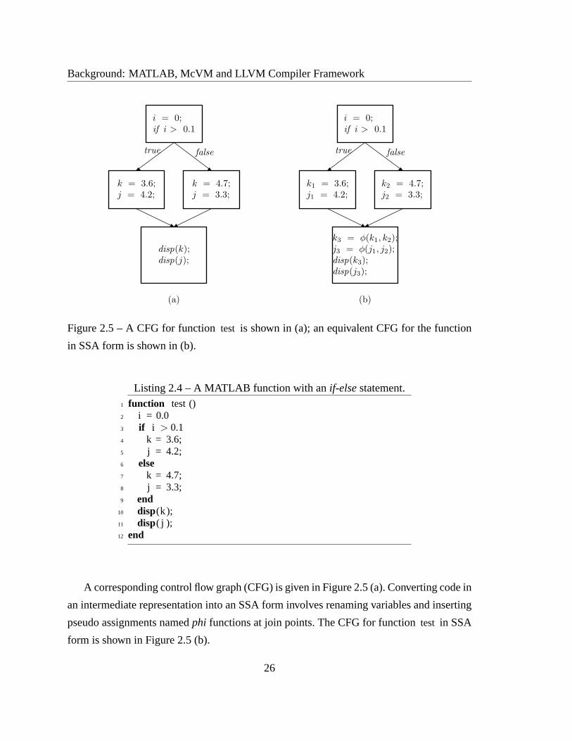
Listing 2.4 – A MATLAB function with anif-elsestatement.1 function test ()2 i = 0.03 if i > 0.14 k = 3.6;5 j = 4.2;6 else7 k = 4.7;8 j = 3.3;9 end
10 disp(k );11 disp( j );12 end
A corresponding control flow graph (CFG) is given in Figure 2.5(a). Converting code in
an intermediate representation into an SSA form involves renaming variables and inserting
pseudo assignments namedphi functions at join points. The CFG for functiontest in SSA
form is shown in Figure 2.5 (b).
26
2.3. The LLVM Compiler Framework
As shown in the figure,phi nodes have been inserted to merge multiple definitions of a
variable that reach the join point (BB4).
Several algorithms [AWZ88, RWZ88, CFR+89, BBH+13] exist to convert code in an
intermediate representation into an SSA form. Minimal SSA form for a function inserts the
minimum number ofphi functions. A function can be converted into minimal SSA formby
computing thedominance frontiers[CFR+89] of all nodes.
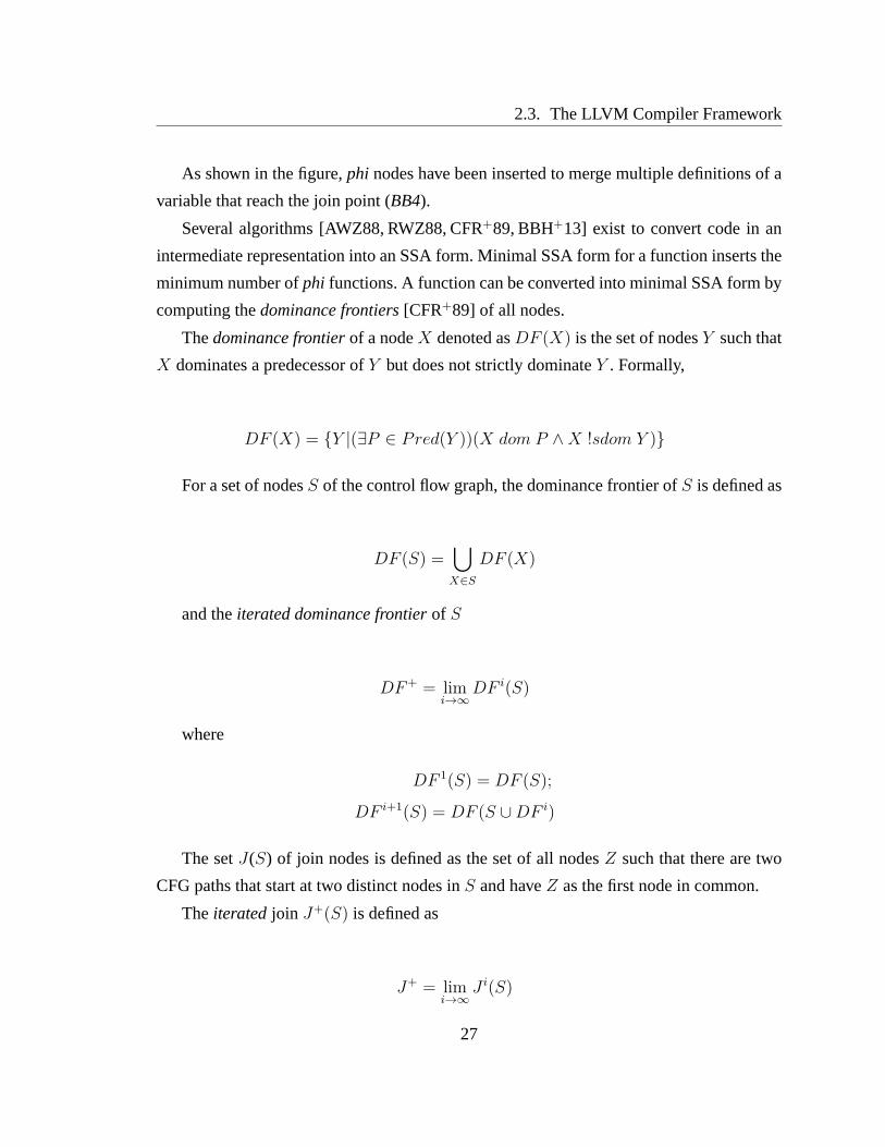
Thedominance frontierof a nodeX denoted asDF (X) is the set of nodesY such that
X dominates a predecessor ofY but does not strictly dominateY . Formally,
DF (X) = {Y |(∃P ∈ Pred(Y ))(X dom P ∧X !sdom Y )}
For a set of nodesS of the control flow graph, the dominance frontier ofS is defined as
DF (S) =⋃
X∈S
DF (X)
and theiterated dominance frontierof S
DF+ = limi→∞
DF i(S)
where
DF 1(S) = DF (S);
DF i+1(S) = DF (S ∪DF i)
The setJ(S) of join nodes is defined as the set of all nodesZ such that there are two
CFG paths that start at two distinct nodes inS and haveZ as the first node in common.
The iteratedjoin J+(S) is defined as
J+ = limi→∞
J i(S)
27

Background: MATLAB, McVM and LLVM Compiler Framework
where
J1 = J(S);
J i+1 = J(S ∪ J i)
Cytron et al. [CFR+89] show that ifS is the set of assignment nodes for a variableV ,
the iterated join ofS is equivalent to the iterated dominance frontier ofS. Thus,DF+(S)
is exactly the set of nodes that needφ nodes for variableV .
We now present examples of code in LLVM IR.
2.3.3 LLVM IR: Examples
In this section, we introduce LLVM IR. Listing 2.5 shows a MATLAB function that re-
turns the sum of its two parameters. A corresponding LLVM IR for the MATLAB function
is shown in Listing 2.6.
Listing 2.5 – A simple MATLAB function.1 function r = addDoubles(arg1, arg2)2 r = arg1 + arg2;3 end
The code uses instructionfadd to add the values of%arg1 and%arg2. The operands of
faddare floating point values.
Listing 2.6 – LLVM IR for addDoubles.1 define double addDoubles(double%arg1, double%arg2) {2 %tmp = fadd double%arg1, %arg23 return double%tmp4 }
To give a hint of the optimizing power of LLVM, we show two semantically equivalent
implementations for the MATLAB function in Listing 2.4. Thefirst is a naive implemen-
tation while the second folds memory operations (load/ store instructions) intoφ nodes to
produce a more efficient implementation oftest.
28

2.3. The LLVM Compiler Framework
Listing 2.7 – A naive implementation oftest (Listing 2.4) in LLVM IR.1 define void @test() {2 entry :3 %i = alloca double4 %j = alloca double5 %k = alloca double6 store double 0.000000e+00, double* %i7 %iVal = load double* %i8 %ifCond = fcmp ogt double%iVal , 1.000000e−019 br i1 %ifCond , label %then, label %else
10
11 then : ; preds =%entry12 store double 3.600000e+00, double* %k13 store double 4.200000e+00, double* %j14 br label %exit15
16 else : ; preds =%entry17 store double 4.700000e+00, double* %k18 store double 3.300000e+00, double* %j19 br label %exit20
21 exit :; preds =%else, %then
22 %nK = load double* %k23 %nJ = load double* %j24 %0 = call i64 @dispDB(double%nK )25 %1 = call i64 @dispDB(double%nJ )26 ret void27 }
In Listing 2.8, all the memory accesses in Listing 2.7 have been converted to register
reads/writes. The LLVM instruction set allows an infinite set of virtual registers.
29

Background: MATLAB, McVM and LLVM Compiler Framework
Listing 2.8 – A more optimized implementation oftest (Listing 2.4) in
LLVM IR.1 define void @test() {2 entry :3 %ifCond = fcmp ogt double 0.000000e+00, 1.000000e−014 br i1 %ifCond , label %then, label %else5
6 then : ; preds =%entry7 br label %exit8
9 else : ; preds =%entry10 br label %exit11
12 exit :; preds =%else, %then
13 %j .0 = phi double [ 4.200000e+00,%then ], [ 3.300000e+00,%else ]14 %k .0 = phi double [ 3.600000e+00,%then ], [ 4.700000e+00,%else ]15 %0 = call i64 @dispDB(double%k .0)16 %1 = call i64 @dispDB(double%j .0)17 ret void18 }
2.3.4 LLVM Transformation and Optimization Pass
LLVM provides a framework for transforming and optimizing code in LLVM IR. Trans-
formations and optimizations are written as passes. An LLVMpass is a subclass ofPass
or its several, similarly named, derived classes, including, BasicBlockPassfor basic block-
level transformations;FunctionPassfor function-level transformations; andModulePassfor
module-level transformations. We shall illustrate how to write an LLVM pass with a
function-level pass.
Suppose we want to count the number of call instructions in a function. One can write
a function-level pass that scans the instructions in the function and updates a counter when
it finds a call instruction.
30
2.3. The LLVM Compiler Framework
Listing 2.9 – An example of a function pass.1 namespace{2 using namespacellvm;3 // counts the number of function calls in a function4 class CallCountPass :public FunctionPass{5 public :6 CallCountPass() : FunctionPass(ID), callCount (0){}7
8 unsignedgetCallCount ()const { return callCount ;}9
10 virtual bool runOnFunction(Function& F){11 countCalls (F);return false ;12 }13
14 virtual const char* getPassName()const {15 return "Call Counter Pass" ;16 }17 static char ID;18 private :19 // counts the number of call instructions in a Function20 void countCalls (Function& F){21 for (Function :: const iterator FI = F.begin (),22 FE = F.end (); FI != FE; ++FI){23 const BasicBlock& BB =*FI;24 for (BasicBlock :: const iterator BI = BB.begin (),25 BE = BB.end(); BI != BE; ++BI){26 const Instruction* I = & *BI;27 if ( isa<CallInst>(I)) ++callCount;28 }}}29 unsignedcallCount ;30 };31
32 FunctionPass* createCallCountPass (){33 return new CallCountPass();}34 char CallCountPass :: ID = 0;35 }
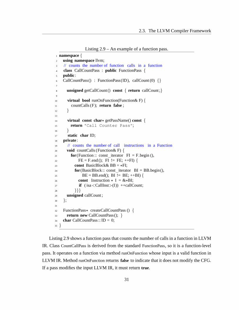
Listing 2.9 shows a function pass that counts the number of calls in a function in LLVM
IR. ClassCountCallPassis derived from the standardFunctionPass, so it is a function-level
pass. It operates on a function via methodrunOnFunctionwhose input is a valid function in
LLVM IR. Method runOnFunctionreturnsfalse to indicate that it does not modify the CFG.
If a pass modifies the input LLVM IR, it must returntrue.
31

Background: MATLAB, McVM and LLVM Compiler Framework
As shown in Listing 2.9, classCountCallPassdefines a private method namedcountCalls.
The method is called byrunOnFunction. In lines 17 – 24,countCallstraverses the CFG and
increments a counter in line 24 if the current instruction isa call instruction. After scanning
all the basic blocks in the function, data membercallCountwill contain the count of all the
call instructions in the analyzed function.
LLVM provides a variety of pass managers to organize and schedule passes to be run
on input code in LLVM IR.FunctionPassManagercan be used to schedule passes to be run
on functions in LLVM IR. For instance, the following code snippet creates a function pass
manager and adds some optimization/transformation passesto the pass manager.
...FunctionPassManager FPM(module);FPM.add(createCountCallPass ());FPM.add(createConstantPropagationPass ());FPM.add(llvm::createPromoteMemoryToRegisterPass());FPM.add(createGVNPass());FPM.add(createEarlyCSEPass());...
In the code snippet, five different passes were submitted to the pass manager (FPM).
The user runs the passes in the order of their creation by calling method run of
FunctionPassManagerand passing the input function such asF in the following code snippet.
A user can also specify dependencies between passes. This can change the order in which
passes are run on an input LLVM IR function.
...FPM.run(*F);...
The call to methodrun will cause all the four passes to be run on functionF.
2.3.5 LLVM JIT Execution Engine
LLVM provides several execution engines that can be used to execute or interpret
LLVM IR. The JIT execution engine allows runtime code generation and is suitable for
32

2.4. Summary
building JIT compilers for dynamic languages. The LLVM framework also has an LLVM
IR interpreter.
To build a JIT compiler for a programming language, a user needs to create a JIT ex-
ecution engine. MethodcreateJITof the classExecutionEnginecan be used to create a JIT
execution engine. A user can also use the classEngineBuilderto create an execution engine.
The following code snippet shows how to useEngineBuilderto create a suitable execution
engine.
Listing 2.10 – Creating a JIT execution engine.1 using namespacellvm;2 ...3 EngineBuilder EB(module);4 EB.setOptLevel(CodeGenOpt::Default);5 EB.setEngineKind(EngineKind::Kind::JIT );6 ExecutionEngine* jitEE = EB.create ();7 ...
In the code snippet shown in Listing 2.10, the statement in line 2 creates an engine
builder. In line 3, the code generation optimization level is set to its default optimization
level. Line 4 sets the execution engine kind to JIT and the statement in line 5 creates a JIT
execution engine using the settings from the engine builderobject (EB).
2.4 Summary
In this section, we introduced the most relevant systems used for the work presented
in the thesis, which is on runtime optimization techniques for implementing the MATLAB
programming language.
The chapter began with an introduction to them MATLAB programming language. We
later introduced McVM— an open-source implementation of MATLAB. McVM is based
on the LLVM compiler framework. We reviewed LLVM at the end ofthe chapter.
LLVM supports JIT compilation and execution via its JIT execution engine. Although
LLVM provides support for recompilation of functions, it does not support on-the-fly opti-
mizations. In other words, a running function cannot be transformed or optimized until all
its instructions have been executed.
33
Background: MATLAB, McVM and LLVM Compiler Framework
In chapters 3 – 8, we present the research work of this thesis,corresponding to the
shaded boxes in Figure 2.1.
34

Chapter 3
Copy Optimization in MATLAB
In the previous chapter, we introduced the MATLAB programming language and its
implementation in McVM. The problem addressed in this chapter is the efficient compila-
tion of the array copy semantics defined by the MATLAB language. The basic semantics
and types in MATLAB are very simple. Every variable is assumed to be an array (scalars
are defined as 1x1 arrays) and copy semantics is used for assignments of one array to an-
other array, parameter passing and for returning values from a function. Thus a statement
of the forma = b semantically means that a copy ofb is made and that copy is assigned
to a. Similarly, for a call of the forma = foo(c) , a copy ofc is made and assigned
to the parameter of the functionfoo , and the return value offoo is copied toa. Naive
implementations take exactly this approach.
In the current implementations of MATLAB, however, the copy semantics is imple-
mented lazily using a reference-count approach. The copiesare not made at the time of the
assignment, rather an array is shared until an update to one of the shared arrays occurs. At
update time (for example a statement of the formb(i) = x ), if the array being updated
(in this caseb) is shared, a copy is generated, and then the update is performed on that
copy. We have verified that this is the approach that Octave open-source system [gnu12]
takes (by examining and instrumenting the source code). We believe that this approach (or
a small variation) is what the Mathworks’ closed-source implementation does based on the
user-level documentation [Mat09b, p. 9-2].
35

Copy Optimization in MATLAB
Although the reference-counting approach reduces unneeded copies at run time, it in-
troduces many redundant checks, requires space for the reference counts, and requires ex-
tra code to update the reference counts. This is clearly costly in a garbage-collected VM,
such as the recently developed McVM, a type-specializing JIT [CBHV10,CB09]. Further-
more, the reference-counting approach may generate a redundant copy during an update
of a shared array via a variable if all the other variables that reference the array are dead
variables.
Thus, our challenge was to develop a static analysis approach, suitable for a JIT com-
piler that could determine which copies were required, without requiring reference counts
and without the expense of dynamic checks. Since we are in thecontext of a JIT compiler,
we developed a staged approach. The first phase applies very simple and inexpensive anal-
yses to determine the obvious cases where copies can be avoided. The second phase tackles
the harder cases, using a pair of more sophisticated static analyses: a forward analysis to
locate all places where an array update requires a copy (necessary copy analysis)and then
a backward analysis that moves the copies to the best location and which may eliminate re-
dundant copies (copy placement analysis). We have implemented our analyses in the McJIT
compiler as structured flow analyses on the low-level AST intermediate representation used
by McJIT.
To demonstrate the applicability of our approach, we have performed several experi-
ments to: (1) demonstrate the behaviour of the reference-counting approaches, (2) to mea-
sure the overhead associated with the dynamic checks in the reference-counting approach,
and (3) demonstrate the effectiveness of our static analysis approach. Our results show that
actual needed copies are infrequent even though the number of dynamic checks can be
quite large. We also show that these redundant checks do contribute significant overheads.
Finally, we show that for our benchmark set, our static approach finds the needed number
of copies, without introducing any dynamic checks.
In this chapter, we first describe how the work presented herefits into McVM project
discussed in the Chapter 2. Then, we describe the simple first-stage analyses followed by
a description of the second-stage forward and backward analyses, with examples. We con-
clude the chapter with a discussion of our experimental results.
36

3.1. Background
3.1 Background
McVM
McJIT
Analyses and Code
Specialization
QuickCheck
Necessary Copy and
Copy Placement Analyses
LLVM Code
Generation
Figure 3.1 – A simplified overview of McJIT (shaded boxes correspond to the analyses
presented in this chapter).
The techniques presented in this chapter have been implemented in McJIT (described
in Section 2.2), a JIT compiler for MATLAB. In Chapter 2, we highlighted how McJIT
specializes code based on the function argument types that occur at run time. When gen-
erating code McJIT assumes reference semantics, and not copy semantics, for assignments
between arrays and parameter passing. That is, arrays are dealt with as pointers and only the
pointers are copied. Clearly this does not match the copy semantics specified for MATLAB
and thus the need for the two shaded boxes in Figure 3.1 in order to determine where copies
are required and the best location for the copies. These two analysis stages are the core of
the techniques presented in this chapter. It is also important to note that the specialization
and type inference in McJIT means that variables that certainly have scalar types will be
stored in LLVM registers and thus the copy analyses only needto consider the remaining
variables.
37

Copy Optimization in MATLAB
In the next section, we introduce the first stage of our approach, which is the
QuickCheck. Following that we introduce the second stage — thenecessary copyandcopy
placementanalyses.
3.2 Quick Check
The QuickCheckphase (QC) is a combination of two simple and fast analyses. The
first, written parameters analysis, is a forward analysis which determines the parameters
that may be modified by a function. The intuition is that during a call of the function,
the arguments passed to it from the caller need to be copied tothe corresponding formal
parameters of the function only if the function may modify the parameters. Read-only
arguments do not need to be copied. For example,
function foo(arg1 , arg2)disp(arg1 );arg2(1) = 1;
end
in function foo above, onlyarg2 of the function needs to be copied. There is no need to
copyarg1since it is only read and not modified byfoo.
The analysis computes a set of pairs, where each pair represents a parameter and the as-
signment statement that last defines the parameter. For example, the entry (p1, d1) indicates
that the last definition point for parameterp1 is statementd1. The analysis begins with a set
of initial definition pairs, one pair for each parameter declaration. The analysis also builds
acopy list, a list of parameters which must be copied, which is initialized to the empty list.
The analysis is a forward flow analysis, using union as the merge operator. The key flow
equations are for assignment statements of two forms:
p = rhs: If the left-hand side (lhs) of the statement is a parameterp, then this statement
is redefiningp, so all other definitions ofp are killed and this new definition ofp is
generated. Note that according to the MATLAB copy semantics, such a statement is
not creating an alias betweenp andrhs, but ratherp is a new copy; subsequent writes
to p will write to this new copy.
38

3.2. Quick Check
p(i) = rhs: If the lhs is an array index expression (i.e., the assignment statement is writing
to an element ofp), and the array symbolp is a parameter, it checks if the initial
definition of the parameter reaches the current assignment statement and if so, it
inserts the parameter into the copy list.
At the end of the analysis, the copy list contains all the parameters that must be copied
before executing the body of the function.
The second analysis iscopy replacement, a standard sort of copy propagation/elimina-
tion algorithm that is similar to the approach used by an APL compiler [Wei85]. It deter-
mines when a copy variable can be replaced by the original variable (copy propagation).
If all the uses of the copy variable can be replaced by the original variable then the copy
statement defining the copy can be removed after replacing all the uses of the copy with the
original (copy elimination).
To illustrate this point, consider the following equivalent code snippets. Variableb in
statement 3 of Box 1
Box 1:
1: a = rand(15000);
2: b = a;
3: c = 2*b
Box 2:
1: a = rand(15000);
2: b = a;
3: c = 2*a;
can be replaced witha as done in Box 2; sinceb is not referenced after statement 3, state-
ment 2 in Box 2 can be removed by the dead-code optimizer.
The copy replacement analysis computes a set of pairs of variables by examining as-
signment statements of the formb = a. A pair represents thelhs andrhs of an assignment
statement, and indicates that if a successor of the statement usesthe first member of the
pair then the variable used could be replaced with the secondmember of the pair. For ex-
ample, if the pair, (b, a) reaches the statementc = 2*b thenb could be replaced witha in
the statement.
Like thewritten parametersanalysis, it is a forward flow analysis. However, in this case
the merge function is intersection. The key flow equations for copy replacement analysis
are:
39

Copy Optimization in MATLAB
b = a if both the lhs and therhs are variables, a new pair of variables, that is, (b, a) is
generated at the statement.
lhs = rhs if lhs is a member of a pair that reaches the statement, such pairs are killed at the
statement. This is because the statement is redefininglhs and its new value may no
longer match that of the other member of the pairs.
At the end of the analysis, the analyzed function is transformed using the result of the
analysis.
If the analysed function does not return an array and all the remaining copy statements
have been made redundant by the QC transformation, then there is no need to apply a more
sophisticated analysis. If copies do remain, however, thenphase 2 is applied, as outlined in
the next two sections.
3.3 Necessary Copy Analysis
Thenecessary copy analysisis a forward analysis that collects information that is used
to determine whether a copy should be generated before an array is modified. To simplify
our description of the analysis, we consider only simple assignment statements of the form
lhs = rhs. It is straightforward to show that our analysis works for both single (onelhsvari-
able) and multiple assignment statements (multiplelhsvariables). We describe the analysis
by defining the following components.
3.3.1 Domain
The domain of the analysis’ flow facts is the set of pairs that comprised of an array refer-
ence variable and the ID of the statement that allocates the memory for the array; henceforth
calledallocators. We write(a, s) if a may reference the array allocated at statements.
3.3.2 Problem Definition
At a program pointp, a variable references a shared array if the number of variables
that reference the array is greater than one. An array updatevia an array reference variable
40

3.3. Necessary Copy Analysis
requires a copy if the variablemay reference a shared array atp and at least one of the
other variables that reference the same array islive afterp. We assume that at each program
point, the set oflive variableshas been computed.
3.3.3 Flow Function
out(Si) = gen(Si) ∪ (in(Si)− kill(Si)).
Given the assignment statements of the forms:
Si : a = alloc (3.1)
Si : a = b (3.2)
Si : a(j) = x (3.3)
Si : a = f(arg1, arg2, ..., argn) (3.4)
whereSi denotes a statement ID;alloc is a new memory allocation performed by statement
Si1; a, b are array reference variables;x is a rvalue; f is a function,arg1, arg2, ..., argn
denote the arguments passed into the function and the corresponding formal parameters are
denoted withp1, p2, ..., pn.
We partitionin(Si) using allocators. The partition,Qi(m), containing flow entries for
allocatorm is:
Qi(m) = {(x, y)|(x, y) ∈ in(Si) ∧ y = m} (3.5)
Now consider statements of type 3.2 above; if variableb has a reaching definition atSi
then there must exist some(b,m) ∈ in(Si) and there exists a non-emptyQi(m) such that
(b,m) ∈ Qi(m).
In addition, if b may reference a shared array atSi then |Qi(m)| > 1. Let us call the
set of all suchQi(m)s,Pi. We writePi(a) for the set ofQis obtained by partitioningin(Si)
using the allocators of variablea.
Considering statements of the form 3.3,Pi(a) 6= ∅ implies that a copy ofa must be
generated before executingSi and in that case,Si is acopy generator. This means that after
this statement,a will point to a new copy and no other variable will refer to this copy.
1. Functions such aszeros, ones, rand andmagicare memory allocators in MATLAB.
41

Copy Optimization in MATLAB
We are now ready to construct a table ofgen and kill sets for the four assignment
statement kinds above. To simplify the table, we define:
Kill define(a) = {(x, s)|(x, s) ∈ in(Si) ∧ x = a}
Kill dead= {(x, s)|(x, s) ∈ in(Si) ∧ not live(Si, x)}
Kill update(a) = {(x, s)|(x, s) ∈ in(Si) ∧ x = a ∧ Pi(a) 6= ∅}
wherelive(Si, x) is a function that returnstrue if variablex is live at program pointSi and
returnsfalse otherwise.
Stmt Gen set Kill set
(3.1) {(x, s)|x = a ∧ s = Si ∧ live(Si, x)} Kill define(a) ∪ Kill dead
(3.2) {(x, s)|x = a ∧ (y, s) ∈ in(Si) ∧ y = b ∧ live(Si, x)} Kill define(a) ∪ Kill dead
(3.3) {(x, s)|x = a ∧ s = Si ∧ Pi(x) 6= ∅} Kill update(a) ∪ Kill deads
(3.4) seegen(f) below Kill define(a) ∪ Kill deads
Computing thegen set for a function call is not straightforward. Certain built-in
functions allocate memory blocks for arrays; such functions are categorized asalloc
functions. A question that arises is: does the return value of the called function reference
the same shared array as a parameter of the function? If the return value references the
same array as a parameter of the function then this sharing must be made explicit in the
caller, after the function call statement. Therefore, thegenset for a function call is defined
as:
gen(f) =
{(a, Si)}, if live(Si, a) and isAllocFunction(f)
{(x, s)|x = a ∧ (argj, s) ∈ in(Si) ∧ live(Si, x)},
if ret(f) aliases paramj(f), 0 < j ≤ size(params(f)),
{(a, Si)}, if ∀(p ∈ params(f)), not (ret(f) aliases p)
{(x, s)|x = a ∧ arg ∈ args(f) ∧ (arg, s) ∈ in(Si) ∧ live(Si, x)},
otherwise (e.g., iff is recursive)
42

3.3. Necessary Copy Analysis
The first alternative generates a flow entry(a, Si) if the rhs is an alloc function and
the lhs (a) is live after statementSi; this makes statementSi an allocator. In the second
alternative, the analysis requests the result of the necessary copy analysis onf from an
analysis manager.2 The manager caches the result of the previous analysis on a given
function. From the result of the analysis onf , we determine the return variables off that
are aliases to the parameters off and hence aliases to the arguments off . This is explained
in detail under the next section on Initialization. The return variable off corresponds
to the lhs (a) in statement type 3.4. Therefore, using the summary information of f , we
generate new flow entries from those associated with the arguments that the return variable
may reference provided thata is alsolive afterSi.
The third alternative generates{(a, Si)}, if the return variable aliases no parameters of
f . The fourth alternative is conservative: new flow entries are generated from those ofall
the arguments tof . This can happen if the call off is recursive orf cannot be analyzed
because it is neither a user-defined function nor analloc function.
We chose a simple strategy for recursion because recursive functions occur rarely in
MATLAB. In a separate study by our group, we found that out of 15,966 functions in 625
projects examined, only 48 functions (0.3%) are directly recursive. None of the programs
in our benchmarks had recursive functions.
Therefore, we expect that the conservative option in the definition of gen(f) above will
be rarely taken in practice.
3.3.4 Initialization
The input set for a function is initialized with a flow entry for each parameter and an
additional flow entry (a shadow entry) for each parameter is also inserted. This is necessary
in order to determine which of the parameters (if any) returnvariable references. We use a
shadow entry to detect when a parameter that has not been assigned to any other variable
is updated. At the entry to a function, the input set is given as
2. This uses the same analysis machinery as the type estimation in McJIT.
43
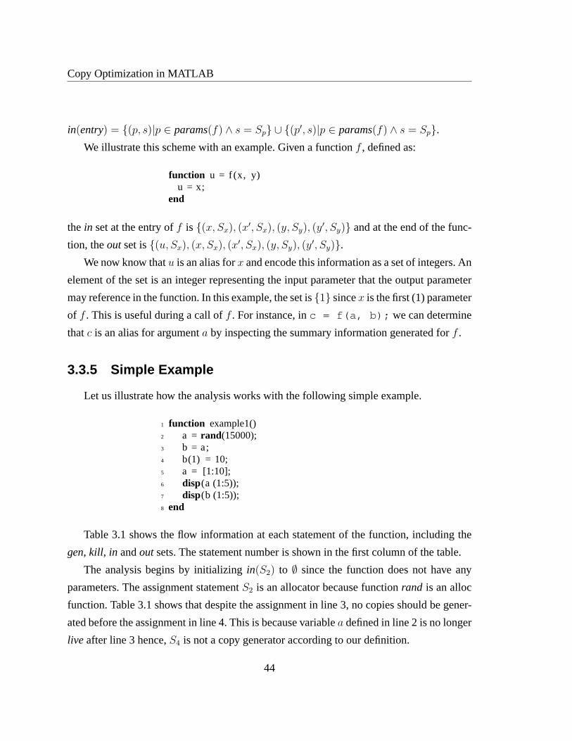
Copy Optimization in MATLAB
in(entry) = {(p, s)|p ∈ params(f) ∧ s = Sp} ∪ {(p′, s)|p ∈ params(f) ∧ s = Sp}.
We illustrate this scheme with an example. Given a functionf , defined as:
function u = f (x, y)u = x;
end
the in set at the entry off is {(x, Sx), (x′, Sx), (y, Sy), (y
′, Sy)} and at the end of the func-
tion, theoutset is{(u, Sx), (x, Sx), (x′, Sx), (y, Sy), (y
′, Sy)}.
We now know thatu is an alias forx and encode this information as a set of integers. An
element of the set is an integer representing the input parameter that the output parameter
may reference in the function. In this example, the set is{1} sincex is the first (1) parameter
of f . This is useful during a call off . For instance, inc = f(a, b); we can determine
thatc is an alias for argumenta by inspecting the summary information generated forf .
3.3.5 Simple Example
Let us illustrate how the analysis works with the following simple example.
1 function example1()2 a = rand(15000);3 b = a;4 b(1) = 10;5 a = [1:10];6 disp(a (1:5));7 disp(b (1:5));8 end
Table 3.1 shows the flow information at each statement of the function, including the
gen, kill , in andoutsets. The statement number is shown in the first column of the table.
The analysis begins by initializingin(S2) to ∅ since the function does not have any
parameters. The assignment statementS2 is an allocator because functionrand is an alloc
function. Table 3.1 shows that despite the assignment in line 3, no copies should be gener-
ated before the assignment in line 4. This is because variablea defined in line 2 is no longer
live after line 3 hence,S4 is not a copy generator according to our definition.
44

3.4. Copy Placement Analysis
# Gen set Kill set In set Out set
2 {(a, S2)} ∅ ∅ {(a, S2)}
3 {(b, S2) {(a, S2)} {(a, S2)} {(b, S2)}
4 ∅ ∅ {(b, S2)} {(b, S2)}
5 {(a, S5) ∅ {(b, S2)} {(b, S2), (a, S5)}
Table 3.1 – Forward Analysis result forexample1.
3.3.6 if-else Statement
So far we have been considering sequences of statements. As our analysis is done di-
rectly on a simplified AST, analyzing anif-else statement simply requires that we analyze
all the alternative blocks and merge the result at the end of the if-else statement using the
merge operator (∪).
3.3.7 Loops
We compute the input set reaching a loop and the output set exiting a loop using stan-
dard flow analysis techniques, that is, we merge the input flowset from the loop’s entry
with the output set from the loop back-edge until a fixed pointis reached.
To analyse a loop more precisely, we implemented a context-sensitive loop analysis that
distinguishes the sharing of arrays that are initiated outside the loop from those initiated
within the loop, and from those initiated in different iterations of the loop. This distinction
is necessary in certain cases to prevent unneeded copies from being generated [LH10].
We found, however, that real MATLAB programs did not requirethe context-sensitivity to
achieve good results. The standard approach is sufficient for typical MATLAB programs.
3.4 Copy Placement Analysis
In the previous section, we described the forward analysis which determines whether
a copy should be generated before an array is updated. One could use this analysis alone
to insert the copy statements, but this may not lead to the best placement of the copies and
45

Copy Optimization in MATLAB
may lead to redundant copies. The backwardcopy placement analysisdetermines a better
placement of the copies, while at the same time ensuring safeupdates of a shared array.
Examples of moving copies include hoisting copies out of if-then constructs and out of
loops.
The intuition behind this analysis is that often it is betterto perform the array copy close
to the statement which created the sharing (i.e. statementsof the forma = b) rather than
just before the array update statements (i.e. statements ofthe forma(i) = b) that require the
copy. In particular, if the update statement is inside a loop, but the statement that created
the sharing is outside the loop, then it is much better to create the copy outside of the loop.
Thus, thecopy placement analysisis a backward analysis that pushes the necessary copies
upwards, possibly as far as the statement that created the sharing.
3.4.1 Abstraction
A copy entry is a three-tuple:
e=< copy loc, var, alloc site> (3.6)
wherecopy loc denotes the ID of the node that generates the copy,var denotes the variable
containing a reference to the array that should be copied, and alloc site is the allocation
site where the array referenced byvar was allocated. We refer to the three components of
the three-tuple ase.copy loc, e.var, ande.alloc site.
LetC denote the set of all copies generated by a function.
Given a function, the analysis begins by traversing the block of statements of the func-
tion backward. The domain of the analysis’ flow entries is theset of copy objects and the
merge operator is intersection (∩).
DefineCout as the set of copy objects at the exit of a block andCin as the set of copy
objects at the entrance of a block. Since the analysis beginsat the end of a function,Cout is
initialized to∅. The rules for generating and placing copies are described here.
46

3.4. Copy Placement Analysis
3.4.2 Statement Sequence
Given a sequence of statements, we are given aCout for this block and the analysis
traverses backwards through the block computing aCin for the block. As each statement is
traversed the following rules are applied for the differentkinds of the assignment statements
in the sequence. The setsin(Si), Qi(m), Pi(a) are defined in Section 3.3.
Rule 1: array updates, Si : a(y) = x : Given that the array variable of thelhs of
statementSi is a, when a statement of this form is reached, we add a copy for each partition
for a shared array to the current copy set. Thus
Cin := Cin ∪
{
∅ if Pi(a) = ∅
{< s, x, y > |s = Si ∧ x = a ∧Qi(y) ∈ Pi(x)} otherwise
Rule 2: array assignments, Sj : a = b : If ∀e ∈ Cin(e.var 6= a and e.var 6= b),
and∀e ∈ Cout(e.var 6= a and e.var 6= b), we skip the current statement. However, if in
the current block,∃e ∈ Cin(e.var= a or e.var= b), we removee from the current copy
flow setCin. This means that the copy has been placed at its current location — the location
specified in copy entrye. Otherwise, if∃e ∈ Cout(e.var= a or e.var= b), we perform the
following:
if Pj(a) = ∅, this is usually the case, we move the copy from the statemente.copy loc
to Sj and removee from the flow set. The copye has now been finally placed.
if Pj(a) 6= ∅, ∀(Qi(m) ∈ Pj(a)), we add a runtime equality test fora against the variable
x (x 6= a) of each member ofQi(m) at the statemente.copy loc. SincePj(a) 6= ∅, there
is at least a definition ofa that reaches this statement and for whicha references a shared
array. In addition, because copye was generated after the current block there are at least
two different paths to statemente.copy loc, the current location ofe. We place a copy ofe
at the current statementSj and removee from the flow set. Note that two copies ofe have
been placed; one ate.copy loc and another atSj. However, runtime guards have also been
placed ate.copy loc, ensuring that only one of these two copies materializes at run time.
The following code snippet illustrates this scenario.
47

Copy Optimization in MATLAB
1 b = [2, 4, 8];2 a = b;3 if (cond)4 c = rand(10);5 ...6 a = c;7 end8 a( i ) = 10;9 disp(a );
10 disp(b );
StatementS2 dominates statementS4; if the then block is taken then, at statementS8
(the array update statement),a will reference the array allocated atS4. Otherwise,a will
reference the array allocated atS1. Thus, by placing a copy afterS6, it is guaranteed thata
is unique if the program takes the path throughS6 to S8; and the update atS8 is therefore
safe and no copy will be generated atS8 because the runtime guard will be false. However,
if this path is not taken, then the guard atS8 will be true and a copy will be generated.
We expect that such guards will not usually be needed, and in fact none of our bench-
marks required any guards.
3.4.3 if -else Statements
Let Cif andCelse denote the set of copies generated in anif and anelse block respec-
tively. First we compute
C ′ := (Cout∩ Celse∩ Cif)
Then we compute the differences
C ′out := Cout \ C
′; C ′else := Celse\ C
′; C ′if := Cif \ C
′
to separate those copies that do not intersect with those in other blocks but should never-
theless be propagated upward. Since the copies in the intersection will be relocated, they
are removed from their current locations.
And finally,
Cin := C ′out∪ C ′
else∪ C ′if ∪ {< s, e.var, e.alloc site> |s = SIF ∧ e ∈ C ′}
48

3.5. Using the Analyses
Note that a copy objecte with its first component set toSIF is attached to theif-elsestate-
mentSIF. That means if these copies remain at this location, the copies should be generated
before theif-elsestatement.
3.4.4 Loops
The main goal here is to identify copies that could be moved out of a loop. To place
copies generated in a loop, we apply the rules for statement sequence and theif-else state-
ment. The analysis propagates copies upward from the inner-most loop to the outer-most
loop and to the main sequence until either loop dependenciesexist in the current loop or it
is no longer possible to move the copy according to Rule 2 in Section 3.4.2.
A disadvantage of propagating the copy outside of the loop isthat if none of the loops
that require copies is executed then we would have generateda useless copy. However, the
execution is still correct. For this reason, we assume that aloop will alwaysbe executed and
generate copies outside loops, wherever possible. This is areasonable assumption because a
loop is typically programmed to execute. With this assumption, there is no need to compute
the intersection ofCloop andCout. Hence
Cin := Cout∪ {< s, e.var, e.alloc site> |s = Sloop∧ e ∈ Cloop})
3.5 Using the Analyses
This section illustrates how the combination of the forwardand the backward analyses
is used to determine the actual copies that should be generated. First consider the following
program,test3. Table 3.2 (a) shows the result of the forward analysis.
49

Copy Optimization in MATLAB
1 function test3 ()2 a = [1:5];3 b = a;4 i = 1;5 if ( i > 2) % I6 a(1) = 100;7 else8 a(1) = 700;9 end
10 a(1) = 200;11 disp(a );12 disp(b );13 end
# Gen set In Out
2 {(a, S2)} ∅ {(a, S2)}
3 {(b, S2)} {(a, S2)} {(a, S2)(b, S2)}
6 {(a, S6)} {(a, S2), (b, S2)} {(b, S2)(a, S6)}
8 {(a, S8)} {(a, S2), (b, S2)} {(b, S2), (a, S8)}
10 ∅ {(b, S2), (a, S6), (a, S8)} {(b, S2), (a, S6), (a, S8)}
(a) Necessary Copy Analysis Result fortest3.
# Cout Cin Current Result
10 ∅ ∅ ∅
8 ∅ {< S8, a, S2 >} {(a, S8)}
6 ∅ {< S6, a, S2 >} {(a, S6)}
I ∅ {< SI , a, S2 >} {(a, SI)}
3 {< SI , a, S2 >} ∅ {(a, SI)}
2 ∅ ∅ {(a, SI)}
(b) Copy Placement Analysis Result fortest3.
Table 3.2 – Necessary Copy and Copy Placement Analyses fortest3.
50

3.5. Using the Analyses
Table 3.2 (b) gives the result of the backward analysis. TheI used in line 5 oftest3
stands for theif-else statement intest3. The analysis begins from line 12 oftest3. The
out setCout is initially empty. At line 10,Cout is still empty. When theif -else statement
is reached, a copy ofCout (∅) is passed to theElseblock and another copy is passed to
the If block. The copy{< S8, a, S2 > is generated in theElseblock because|Q(S2) =
{(a, S2), (b, S2)}| = 2, hencePi(a) 6= ∅. Similarly < S6, a, S2 > is generated in theIf
block.
By applying the rule forif-else statement described in Section 3.4.3, the outputs of theIf
and theElseblocks are merged to obtain the result atSI (the if-else statement). Applying
Rule 2 for statement sequence (Section 3.4.2) inS3, < SI , a, S2 > is removed fromCin
and the analysis terminates atS2. The final result is that a copy must be generated before
the if -else statement instead of generating two copies, one in each block of the if -else
statement. This example illustrates how common copies generated in the alternative blocks
of anif-else statement could be combined and propagated upward to reducecode size.
The second example,tridisolveis a MATLAB function from [Cle04]. The forward anal-
ysis information is shown in Table 3.3. The table shows thegenandin sets at each relevant
assignment statement oftridisolve. The results in different loop iterations are shown using
a subscript to represent loop iteration. For example, the row number252 refers to the result
at the statement labelledS25 in the second iteration. The analysis reached a fixed point after
the third iteration.
51

Copy Optimization in MATLAB
Listing 3.1 – A MATLAB function (tridisolve).
function x = tridisolve (a,b,c,d)% TRIDISOLVE Solve tridiagonal system of equations .20: x = d;21: n = length(x );
for j = 1:n−1 %F 1mu = a(j )/ b( j );
25: b( j+1) = b( j+1)− mu*c(j);26: x( j+1) = x( j+1)− mu*x(j);
end29: x(n) = x(n)/b(n);
for j = n−1:−1:1 %F 231: x( j ) = (x( j)−c(j)* x( j +1))/b( j );
end
At the function’s entry, thein set is initialized with two flow entries for each parameter
of the function as outlined in Section 3.3. The analysis continues by generating thegen,
in andout sets according to the rules specified in Section 3.3. Notice that statementS25 is
an allocator becauseP25(b) 6= ∅ since|Q25(Sb)| = |{(b, Sb, 0), (b′, Sb, 0)}| > 1. Similarly,
S26 andS29 are also allocators. This means that generating a copy of thearray referenced
by the variableb just before executing the statementS25 ensures a safe update of the array.
The same is true of the array referenced by the variablex in lines 26 and 29. However, are
these the best points in the program to generate those copies? Could the number of copies
be reduced? We provide the answers to these questions when weexamine the results of the
backward analysis.
Table 3.4 shows the copy placement analysis information at each relevant statement of
tridisolve. Recall that the placement analysis works by traversing the statements in each
block of a function backward. In the case oftridisolve, the analysis begins in line 31 in
the secondfor loop of the function. The setCout is passed to the loop body and is initially
empty. The setCin stores all the copies generated in the block of thefor statement. Line 31
is neither a definition nor an allocator, therefore no changes are recorded at this stage of the
analysis.
52

3.5. Using the Analyses
# Gen In
20 {(x, Sd, 0)} {(a, Sa, 0), (a′, Sa, 0), (b, Sb, 0), (b
′, Sb, 0), (c, Sc, 0), (c′, Sc, 0),
(d, Sd, 0), (d′, Sd, 0)}
251 {(b, S25, 1)} {(a, Sa, 0), (a′, Sa, 0), (b, Sb, 0), (b
′, Sb, 0), (c, Sc, 0), (c′, Sc, 0),
(d′, Sd, 0), (x, Sd, 0)}
261 {(x, S26, 1)} {(a, Sa, 0), (a′, Sa, 0), (b
′, Sb, 0), (c, Sc, 0), (c′, Sc, 0), (d
′, Sd, 0),
(x, Sd, 0), (b, S25, 1)}
252 {(b, S25, 2)} {(a, Sa, 0), (a′, Sa, 0), (b, Sb, 0), (b
′, Sb, 0), (c, Sc, 0), (c′, Sc, 0),
(d′, Sd, 0), (x, Sd, 0), (b, S25, 1), (x, S26, 1)}
262 {(x, S26, 2)} {(a, Sa, 0), (a′, Sa, 0), (b
′, Sb, 0), (c, Sc, 0), (c′, Sc, 0), (d
′, Sd, 0),
(x, Sd, 0), (b, S25, 2), (x, S26, 1)}
253 {(b, S25, 3)} {(a, Sa, 0), (a′, Sa, 0), (b, Sb, 0), (b
′, Sb, 0), (c, Sc, 0), (c′, Sc, 0),
(d′, Sd, 0), (x, Sd, 0), (b, S25, 2), (x, S26, 2)}
263 {(x, S26, 3)} {(a, Sa, 0), (a′, Sa, 0), (b
′, Sb, 0), (c, Sc, 0), (c′, Sc, 0), (d
′, Sd, 0),
(x, Sd, 0), (b, S25, 3), (x, S26, 2)}
29 {(x, S29, 0)} {(a′, Sa, 0), (b, Sb, 0), (b′, Sb, 0), (c, Sc, 0), (c
′, Sc, 0), (d′, Sd, 0),
(x, Sd, 0), (b, S25, 3), (x, S26, 3)}
311 ∅ {(a′, Sa, 0), (b, Sb, 0), (b′, Sb, 0), (c, Sc, 0), (c
′, Sc, 0), (d′, Sd, 0),
(b, S25, 3), (x, S29, 0)}
312 ∅ {(a′, Sa, 0), (b, Sb, 0), (b′, Sb, 0), (c, Sc, 0), (c
′, Sc, 0), (d′, Sd, 0),
(b, S25, 3), (x, S29, 0)}
Table 3.3 – Necessary Copy Analysis Result.
53
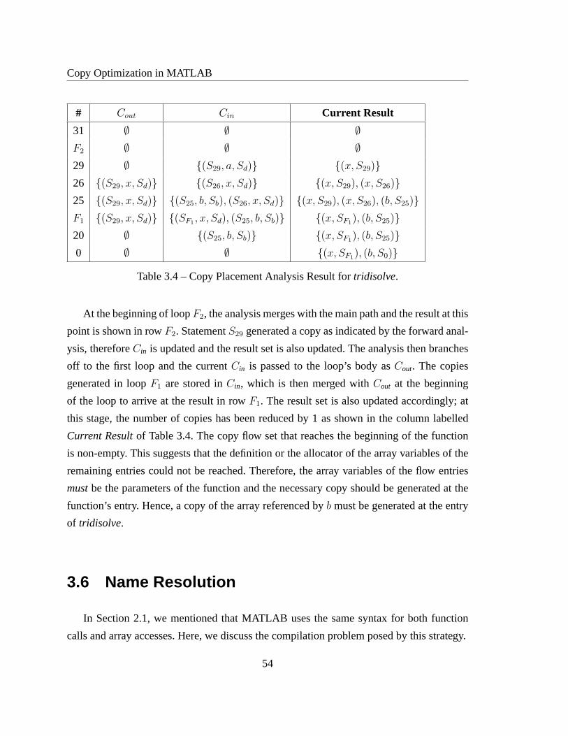
Copy Optimization in MATLAB
# Cout Cin Current Result
31 ∅ ∅ ∅
F2 ∅ ∅ ∅
29 ∅ {(S29, a, Sd)} {(x, S29)}
26 {(S29, x, Sd)} {(S26, x, Sd)} {(x, S29), (x, S26)}
25 {(S29, x, Sd)} {(S25, b, Sb), (S26, x, Sd)} {(x, S29), (x, S26), (b, S25)}
F1 {(S29, x, Sd)} {(SF1, x, Sd), (S25, b, Sb)} {(x, SF1
), (b, S25)}
20 ∅ {(S25, b, Sb)} {(x, SF1), (b, S25)}
0 ∅ ∅ {(x, SF1), (b, S0)}
Table 3.4 – Copy Placement Analysis Result fortridisolve.
At the beginning of loopF2, the analysis merges with the main path and the result at this
point is shown in rowF2. StatementS29 generated a copy as indicated by the forward anal-
ysis, thereforeCin is updated and the result set is also updated. The analysis then branches
off to the first loop and the currentCin is passed to the loop’s body asCout. The copies
generated in loopF1 are stored inCin, which is then merged withCout at the beginning
of the loop to arrive at the result in rowF1. The result set is also updated accordingly; at
this stage, the number of copies has been reduced by 1 as shownin the column labelled
Current Resultof Table 3.4. The copy flow set that reaches the beginning of the function
is non-empty. This suggests that the definition or the allocator of the array variables of the
remaining entries could not be reached. Therefore, the array variables of the flow entries
mustbe the parameters of the function and the necessary copy should be generated at the
function’s entry. Hence, a copy of the array referenced byb must be generated at the entry
of tridisolve.
3.6 Name Resolution
In Section 2.1, we mentioned that MATLAB uses the same syntaxfor both function
calls and array accesses. Here, we discuss the compilation problem posed by this strategy.
54

3.7. Experimental Results
An obvious advantage of using identical syntax is that a datastructure initially im-
plemented as an array could be re-implemented as a function without changing the array
accesses. A disadvantage of this strategy, however, is thatit makes it difficult to determine
statically whether an expression is a function call or an array access, thus making analyses
too conservative. For instance, in the statement below, isb a function or an array?
m = b(c, d);
Without a suitable analysis, it is hard to tell whetherb(c, d) is a function call or an array
access. The forward analysis described in Section 3.3 relies on the McVM type inference
analysis [CBHV10, CB09] to determine the type of a symbol. In the simple assignment
statement above, the analysis needs to know whether the variablesm, c andd are arrays.
Furthermore, ifb is a function andm, c andd are arrays, the analysis needs to know whether
m references the same array asc or d. The forward analysis requests the type information
of b and proceeds to analyseb if the result of the look-up indicates thatb is a function.
3.7 Experimental Results
To evaluate the effectiveness of our approach, we set up experiments using benchmarks
collected from disparate sources, including those from [RGG+96,Cle04,Pre86]. Table 3.5
gives a short description of each benchmark, together with,a summary of the results of our
analyses, which we discuss in more detail in the following subsections. For all the experi-
ments described in this chapter, we ran the benchmarks with their smallest input size on an
AMD Athlon™ 64 X2 Dual Core Processor 3800+, 4GB RAM computer running Linux
operating system; GNU Octave, version 3.2.4; MATLAB, version 7.9.0.529 (R2009b)3 and
McVM/McJIT, version 0.5.
The purpose of our experiments was three-fold. First, we wanted to measure the number
of array updates and copies performed by the benchmarks at run time using existing sys-
tems (Section 3.7.1). Knowing the number of updates gives anidea of how many dynamic
checks a reference-counting-based (RC) scheme for lazy copying, such as used by Octave
3. We used the later versions of MATLAB for the experiments described in the following chapters.
55

Copy Optimization in MATLAB
and Mathworks’ MATLAB, need to perform. Recall that our approach does not usually
require any dynamic checks. Knowing the number of copies generated by such systems al-
lows us to verify that our approach does not increase the number of copies as compared to
the reference-counting-based approaches. Secondly, we would like to measure the amount
of overhead generated in reference-counting-based systems (Section 3.7.2). Finally, we
would like to assess the impact of our static analyses in terms of their ability to minimize
the number of copies (Section 3.7.3).
3.7.1 Dynamic Counts of Array Updates and Copies
Our first measurements were designed to measure the number ofarray updates and
array copies that are required by existing reference-counting-based systems, Octave and
Mathworks’ MATLAB. Since we had access to the open-source Octave system we were
able to instrument the interpreter and make the measurements directly. However, the Math-
works’ implementation of MATLAB is a proprietary system andthus we were unable to
instrument it to make direct measurements. Instead, we developed an alternative approach
by instrumenting the benchmark programs themselves via aspects using our ASPECTMAT-
LAB compileramc [ADDH10]. Our aspect4 defines all the patterns for the relevant points
in a MATLAB program including all array definitions, array updates, and function calls.
It also specifies the actions that should be taken at these points in the source program. In
effect, the aspect computes all of the information that a reference-counting-based scheme
would have, and thus can determine, at run time, when an arrayupdate triggers a copy be-
cause the number of references to the array is greater than one. The aspect thus counts all
array updates and all copies that would be required by a reference-counting-based system.
4. This aspect is available at: http://www.sable.mcgill.ca/mclab/copy analysis.html. It is also listed in
Appendix B.5. The benchmarks are also available at: www.sable.mcgill.ca/mclab/mcvm mcjit.html.
56

3.7. Experimental Results
# Copies
# Array Lower Bound With Analyses
Benchmark Updates Aspect Octave Naive QC CA
adpt adaptive quadrature us-
ing Simpson’s rule
19624 0 0 12223 12223 0
capr capacitance of a trans-
mission line using finite
difference and Gauss-
Seidel iteration
9790800 10000 10000 40000 20000 10000
clos transitive closure of a di-
rected graph
2954 0 0 2 2 0
crni Crank-Nicholson so-
lution to the one-
dimensional heat equa-
tion
21143907 4598 6898 11495 6897 4598
dich Dirichlet solution to
Laplace’s equation
6935292 0 0 0 0 0
fdtd 3D FDTD of a hexahe-
dral cavity with conduct-
ing walls
803 0 0 5400 5400 0
fft fast fourier transform 44038144 1 1 2 2 1
fiff finite-difference solution
to the wave equation
12243000 0 0 0 0 0
mbrt Mandelbrot set 5929 0 0 0 0 0
nb1d N-body problem coded
using 1d arrays for the
displacement vectors.
55020 0 0 10984 10980 0
nb3d N-body problem coded
using 3d arrays for the
displacement vectors.
4878 0 0 5860 5858 0
nfrc computes a newton frac-
tal in the complex plane
-2..2,-2i..2i
12800 0 0 6400 6400 0
trid Solve tridiagonal system
of equations
2998 2 2 5 2 2
Table 3.5 – Benchmarks and the results of the copy analysis5
57
Copy Optimization in MATLAB
In Table 3.5 the column labelled# Array Updatesgives the total number of array up-
dates executed. The column# Copiesshows the number of copies generated by the bench-
marks under Octave (reported asOctavein the table) and MATLAB (column labelledAs-
pect). The column# Copiesis split into two:Lower BoundandWith Analyses. The num-
ber of copies generated by Octave and MATLAB (Aspect) are considered the expected
lower bounds (since they perform copies lazily, and only when required) and are therefore
grouped underLower Boundin the table.6
At a high-level, the results in Table 3.5 show that our benchmarks often perform a
significant number of array updates, but very few updates trigger copies. We observed
that no copies were generated in ten out of the thirteen benchmarks. This low rate for
array copies is not surprising because MATLAB programmers tend to avoid copying large
objects and often only read from function parameters.With Analysesis comprised of three
columns,Naive, QC, andCA representing respectively, the number of copies generatedin
our naive system, with the QC phase, and with the copy analysis phase. We return to these
results in Section 3.7.3.
3.7.2 The Overhead of Dynamic Checks
With the reference-counting-based approaches, a dynamic check is needed for each
array update, in order to test if a copy is needed. Our counts indicated that several of our
benchmarks had a high number of updates, but no copies were required. We wanted to
measure the overhead for all of these redundant dynamic checks. The ideal measurement
would have been to time the redundant checks in a JIT-based system that used reference-
counting, such as Mathworks’ MATLAB. Unfortunately we do nothave access to such a
system. Instead we performed two similar experiments, as reported in Table 3.6, for three
benchmarks with a high number of updates and no required copies (dich , fiff and
mbrt ).
6. Note that for the benchmarkcrni Octave performs 6898 copies, whereas the lower bound according
to the Aspect is 4598. We verified that Octave is doing some spurious copies in this case, and that the Aspect
number is the true lower bound.
58

3.7. Experimental Results
McVM Octave(O)
McJIT McJIT(+RC) Overhead(%) Time(s) Overhead
Bmark t(s) # LLVM t(s) # LLVM time size O(+RC) O(-RC) (%)
dich 0.18 546 0.27 625 47.37 14.47 425.05 408.08 4.16
fiff 0.39 388 0.52 415 33.72 6.96 468.64 438.69 6.83
mbrt 5.06 262 5.65 271 11.69 3.44 34.91 31.95 9.29
Table 3.6 – Overhead of Dynamic Checks.
We first created a version of Octave that does not insert dynamic checks before array
update statements. In general this is not safe, but for thesethree benchmarks we knew no
copies were needed, and thus removing the checks allowed us to measure the overhead
without breaking the benchmarks. The column labelledO(+RC) gives the execution time
with dynamic checks and the column labelledO(-RC)gives the times when we artificially
removed the checks. The difference gives us the overhead, which is between 4% and 9%
for these benchmarks. Although this is not a huge percentage, it is not negligible. Further-
more, we felt that the absolute time for the checks was significant and would be even more
significant in a JIT system which has many fewer other overheads.
To measure overheads in a JIT context, we modified McJIT to include enough
reference-counting machinery to measure the overhead of the checks (remember that
McVM is garbage-collected and does not normally have reference counts). For the mod-
ified McVM we added a field to the array object representation to store reference counts
(which is set to zero for the purposes of this experiment) andwe generated LLVM code
for a runtime check before each array update statement. Table 3.6 shows, in time and code
size, the amount of overhead generated by redundant checks.The column labelledMcJIT
is the original McJIT and the column labelledMcJIT(+RC)is the modified version with the
added checks. We measured code size using the number of LLVM instructions (# LLVM)
and execution time overhead in seconds. For these benchmarks the code size overhead was
3% to 14% and the running time overhead ranged from 12% to 47%.
Our conclusions is that the dynamic checks for a reference-counting-based scheme can
be quite significant in both execution time and code size, especially in the context of a JIT.
Thus, although the original motivation of our work was to enable a garbage-collected VM
59

Copy Optimization in MATLAB
that did not require reference counts, we think that our analyses could also be useful to
eliminate unneeded checks in reference-counting-based systems.
3.7.3 Impact of our Analyses
Let us now return to the number of copies required by our analyses, which are given
in the last three columns of Table 3.5. As a reminder, our goalwas to achieve the same
number of copies as the lower bound.
The column labelledNaivegives the number of copies required with a naive imple-
mentation of MATLAB ’s copy semantics, where a copy is inserted for each parameter, each
return value and each copy statement, where thelhs is an array. Clearly this approach leads
to many more copies than the lower bound.
The column labelledCAgives the number of copies when both phases of our static anal-
yses are enabled. We were very pleased to see that for our benchmarks, the static analyses
achieved the same number of copies as the lower bound, without requiring any dynamic
checks. The column labelledQC shows the number of copies when only the QuickCheck
phase is enabled. Although the QuickCheck does eliminate many unneeded copies, it does
not achieve the lower bound. Thus, the second stage is reallyrequired in many cases.
Figure 3.2 – The total bytes of array data copied by the benchmarks under the three options.
To show the impact copies have on execution performance, we measured the total bytes
of array data copied by a benchmark together with its corresponding execution time. These
are shown in Figure 3.2 and Table 3.7 forNaive, QC andCA. The columnsNaiveQC
andNaiveCA
60

3.7. Experimental Results
Bmark Naive QC CA NaiveQC
NaiveCA
adpt 1.57 1.57 1.61 1.00 0.98
capr 1.54 0.91 0.58 1.70 2.66
clos 0.49 0.49 0.48 0.99 1.01
crni 135.09 140.35 131.62 0.96 1.03
dich 0.18 0.18 0.18 1.00 1.00
fdtd 3.79 3.78 2.80 1.00 1.35
fft 1.50 1.50 1.47 1.00 1.02
fiff 0.39 0.39 0.39 0.99 0.99
mbrt 5.06 5.12 5.04 0.99 1.00
nb1d 0.48 0.48 0.45 1.00 1.07
nb3d 0.48 0.48 0.36 1.00 1.35
nfrc 3.23 3.23 3.25 1.00 0.99
trid 1.57 1.04 1.02 1.51 1.53
Table 3.7 – Benchmarks against the total execution times in seconds.
of Table 3.7 show respectively how many times QC and CA performbetter thanNaive. The
table shows thatCA generally outperformsQC and Naive. Copying large arrays affects
execution performance and the results in Table 3.7 validatethis claim. Where a significant
number of bytes were copied by the naive implementation, forexample,capr, crni and
fdtd, CA performs better than bothNaive and QC. In the three benchmarks that do not
generate copies, the performance ofCA is comparable toNaiveandQC. This shows that
the overhead ofCA is low. It is therefore clear from the results of our experiments that
the naive implementation generates significant overhead and is therefore unsuitable for a
high-performance system.
Impact of the First Phase We measured the number of functions that are completely
resolved by the first phase of our approach — in terms of findingall the necessary copies re-
quired to guarantee copy semantics. We found that out of the 23 functions in the benchmark
set, the first stage (i.e., QuickCheck) was only able to resolve about 17% of the functions.
None of the benchmarks was resolved completely by QC. The mainreason for this poor
61

Copy Optimization in MATLAB
performance is that the first phase cannot resolve functionsthat return arrays to their callers.
Like most MATLAB programs, most of the functions in the benchmarks return arrays. This
really shows that the second stage is actually required to completely determine the needed
copies by typical MATLAB programs.
So, the bottom line is that a very low fraction of array updates result in copies, and
frequently no copies are necessary. For our benchmark set, our static analysis determined
the needed number of copies, while at the same time avoiding all the overhead of dynamic
checks. Furthermore, our approach does not require reference counting and thus enables an
efficient implementation of array copy semantics in garbage-collected systems like McVM.
3.8 Summary
In this chapter we have presented an approach for using static analysis to determine
where to insert array copies in order to implement the array copy semantics in MATLAB.
Unlike previous approaches, which used a reference-counting scheme and dynamic checks,
our approach is implemented as a pair of static analysis phases in the McJIT compiler. The
first phase implements simple analyses for detecting read-only parameters and standard
copy elimination, whereas the second phase consists of a forwardnecessary copy analysis
that determines which array update statements trigger copies, and a backwardcopy place-
ment analysisthat determines good places to insert the array copies. All of these analyses
have been implemented as structured-based analyses on the McJIT intermediate represen-
tation.
Our approach does not require frequent dynamic checks, nor do we need the space and
time overheads to maintain the reference counts. Our approach is particularly appealing in
the context of a garbage-collected VM, such as the one we are working with. However,
similar techniques could be used in a reference-counting-based system to remove redun-
dant checks. Our experimental results validate that, on ourbenchmark set, we do not intro-
duce any more copies than the reference-counting approach,and we eliminate all dynamic
checks.
62

Chapter 4
A Modular Approach to On-Stack
Replacement in LLVM
Virtual machines (VMs) with Just-in-Time (JIT) compilers have become common place
for a wide variety of languages. Such systems have an advantage over static compilers in
that compilation decisions can be made on-the-fly and they can adapt to the characteristics
of the running program. On-stack replacement (OSR) is one approach that has been used to
enable on-the-fly optimization of functions/methods [HCU92,FQ03,PVC01,SK06]. A key
benefit of OSR is that it can be used to interrupt a long-running function/method (without
waiting for the function to complete), and then restart an optimized version of the function
at the program point and state at which it was interrupted.
As mentioned in Chapter 2, LLVM is an open compiler infrastructure that can be used
to build JIT compilers for VMs [LA04, llv12]. It supports a well-defined code representa-
tion known as the LLVM IR, as well as supporting a large number of optimizations and
code generators. LLVM has been used in production systems, as well as in many research
projects. For instance, MacRuby is an LLVM-based implementation of Ruby on Mac OS
X core technologies1; Rubinius2 is another implementation of Ruby based on LLVM JIT.
Unladen-swallow is a fast LLVM implementation of Python.3 VMKit 4 is an LLVM-based
1. http://macruby.org/2. http://rubini.us/3. http://code.google.com/p/unladen-swallow/4. Previously http://vmkit.llvm.org/ and now http://vmkit2.gforge.inria.fr/
63

A Modular Approach to On-Stack Replacement in LLVM
project that works to ease the development of new language VMs, and which has three
different VMs currently developed (Java, .Net, and a prototype R implementation). A com-
mon theme of these diverse projects is that they could benefitfrom further on-the-fly op-
timizations, but unfortunately LLVM does not support OSR-based optimizations. Indeed,
we agree with the developers of VMKit who believe that using OSR would enable them
to speculate and develop runtime optimizations that can improve the performance of their
VMs. 5 Thus, given the value of and need for OSR and the wide-spread adoption of LLVM
in both industry and academia, our research work aims to fill this important void and pro-
vide an approach and modular implementation of OSR for LLVM.
Implementing OSR in a non-Java VM and general-purpose compiler toolkits such as
LLVM requires novel approaches. Some of the challenges to implementing OSR in LLVM
include:
(1) Deciding at what point should the program be interrupted andhow should such points
be expressed within the existing design of LLVM, without changing the LLVM IR.
(2) The static single-assignment (SSA) nature of the LLVM IR requires correct updates of
control flow graphs (CFGs) of LLVM code, thus program transformations to handle
OSR-related control flow must be done carefully and fit into thestructure imposed
by LLVM.
(3) LLVM generates a fixed address for each function; how then should the code of a
new version of the running function be made accessible at theold address without
recompiling the callers of the function? This was actually aparticularly challenging
issue to solve.
(4) The OSR implementation must provide a clean integration with LLVM’s capabilities
for function inlining.
(5) As there are many users of LLVM, the OSR implementation should not require modi-
fications to the existing LLVM installations. Ideally the OSR implementation could
just be added to an LLVM installation without requiring any recompilation of the
installation.
5. Private communication with the authors, October 2012.
64
4.1. OSR Classification
We addressed these and other challenges by developing a modular approach to imple-
menting OSR that fits naturally in the LLVM compiler infrastructure.
To illustrate a typical use of our OSR implementation, we have used the implemen-
tation to support a selective dynamic inlining optimization in a MATLAB VM. MAT-
LAB [Mat09b] is a popular platform for programming scientific applications [Mol06]. It is
a dynamic language designed for manipulation of matrices and vectors, which are common
in scientific applications [Cle04]. The dynamic features of the language, such as dynamic
typing and loading, contribute to its appeal but also make anefficient compilation difficult.
MATLAB programs often have potentially long-running loops, and because its optimiza-
tion can benefit greatly from on-the-fly information such as types and array shapes, we
believe that it is an ideal language for OSR-based optimizations. Thus, we wanted to ex-
periment with this idea in McVM/McJIT [CBHV10,McL12], an opensource VM and JIT
for MATLAB, which is built upon LLVM.
The main contributions of this chapter are:
Modular OSR in LLVM: We have designed and implemented OSR for LLVM. Our ap-
proach provides a clean API for JIT compiler writers using LLVM and clean imple-
mentation of that API, which integrates seamlessly with thestandard LLVM distri-
bution and that should be useful for a wide variety of applications of OSR.
Integrating OSR with inlining in LLVM: We show how we handle the case where the
LLVM inliner inlines a function that contains OSR points.
The rest of the chapter is organized as follows. In Section 4.1, we classify OSR tech-
niques according to their runtime transition capabilities. In Section 4.2, we outline the
application programming interface (API) and demonstrate the usage of our OSR module,
from a JIT compiler writer’s point of view. In Section 4.3, wedescribe the implementation
of our API and the integration of inlining. We conclude the chapter in Section 4.4.
4.1 OSR Classification
The term OSR is used in the literature [HCU92, PVC01, FQ03, AAB+05, SK06] to
describe a variety of similar, but different, techniques for enabling an on-the-fly transition
65

A Modular Approach to On-Stack Replacement in LLVM
from one version of running code to another semantically equivalent version. To see how
these existing techniques relate to each other, and to our proposed OSR implementation,
we propose a classification of OSR transitions, as illustrated in Figure 4.1.
base opt1 opt2 · · ·
Optimize
OSR
Deoptimize
OSR
Reoptimize
OSR
Last− vers
ion
OSR
Figure 4.1 – OSR classification.
In most systems with OSR support, the execution of the running code often begins
with interpretation or the execution of the code compiled bya non-optimizing base-line
compiler. We refer to this version of the running code as thebaseversion. This is shown in
the darker shaded block of Figure 4.1.
We call an OSR transition from thebaseversion to more optimized code (such asopt1
in Figure 4.1) anOptimize OSR. The OSR support in the Java HotSpot server compiler
[PVC01] uses this kind of transition.
Some virtual machines allow an OSR transition from optimized code such asopt1 in
Figure 4.1 to unoptimized code (thebaseversion). We call this aDeoptimize OSRtran-
sition. This was the original OSR transition pioneered by Holzle et al. [HCU92] to allow
online debugging of optimized code in the SELF [CU91] virtualmachine.
Systems such as the Jikes RVM [AAB+05], V8 VM 6, and JavaScriptCore7 support
bothOptimize OSRandDeoptimize OSRtransitions. Once a system has deoptimized back
to the base code, it can potentially trigger anotherOptimize OSR, perhaps at a higher-level
of optimization.
We call a transition from optimized code such asopt1 to more optimized code such
as opt2 in Figure 4.1 aReoptimize OSR. Further, we call an OSR transition from more
6. https://developers.google.com/v8/7. http://trac.webkit.org/wiki/JavaScriptCore/
66

4.2. The OSR API
optimized code (e.g.,opt2) to the last version of less optimized code (e.g.,opt1) a Last-
version OSR.
The OSR technique presented in this chapter supports both OSR transitions to a more
optimized version and deoptimizations to the last version.Thus, if one starts with the base
code, our OSR machinery can be used to perform anOptimize OSRtransition. From that
state, our OSR machinery can be used either as aDeoptimize OSRtransition to return to the
base code (which is the last version of the code), or as aReoptimize OSRto transition to an
even more optimized version. Our OSR implementation alwayscaches the last version of
the code, so it can also be used to support aLast-version OSRto transition from a higher-
level of optimization to the previous level.
We now present the API of our OSR implementation8.
4.2 The OSR API
The key objective of this work was to build a modular system with a clean interface that
is easy to use for VM and JIT compiler writers. In this section, we present the API of our
OSR module and how JIT compiler developers who are already building JITs/VMs with
LLVM can use our module to add OSR functionality to their existing JITs. We provide some
concrete examples, based on our McJIT implementation of OSR-based dynamic inlining.
Figure 4.2(a) represents the structure of a typical JIT developed using LLVM.LLVM
CodeGenis the front-end that produces LLVM IR for the JIT. The JIT compiler may per-
form transformations on the IR via theLLVM Optimizer. This is typically a collection of
transformation and optimization passes that are run on the LLVM IR. The output (i.e., the
transformed LLVM IR) from the optimizer is passed to the target code generator,Target
CodeGen, that produces the appropriate machine code for the code in LLVM IR.
In Figure 4.2(b), we show a JIT (such as that shown in Figure 4.2(a)) that has been
retrofitted with OSR support components (the shaded components). We describe the func-
tions of InserterandOSR Passshown in Figure 4.2(b) shortly. In Section 4.3, we present
8. Available at http://www.sable.mcgill.ca/mclab/mcosr/
67
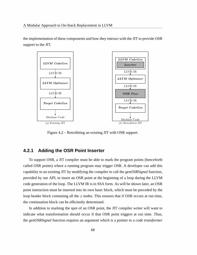
A Modular Approach to On-Stack Replacement in LLVM
the implementation of these components and how they interact with the JIT to provide OSR
support to the JIT.
LLVM CodeGen
LLVM Optimizer
LLVM IR
Target CodeGen
LLVM IR
Machine Code
(a) Existing JIT
LLVM CodeGen
InserterInserter
LLVM Optimizer
LLVM IR
OSR PassOSR Pass
LLVM IR
Target CodeGen
LLVM IR
Machine Code(b) Retrofitted JIT
Figure 4.2 – Retrofitting an existing JIT with OSR support.
4.2.1 Adding the OSR Point Inserter
To support OSR, a JIT compiler must be able to mark the program points (henceforth
called OSR points) where a running program may trigger OSR. A developer can add this
capability to an existing JIT by modifying the compiler to call the genOSRSignalfunction,
provided by our API, to insert an OSR point at the beginning ofa loop during the LLVM
code generation of the loop. The LLVM IR is in SSA form. As willbe shown later, an OSR
point instruction must be inserted into its own basic block,which must be preceded by the
loop header block containing all theφ nodes. This ensures that if OSR occurs at run time,
the continuation block can be efficiently determined.
In addition to marking the spot of an OSR point, the JIT compiler writer will want to
indicate what transformation should occur if that OSR pointtriggers at run time. Thus,
thegenOSRSignalfunction requires an argument which is a pointer to acode transformer
68
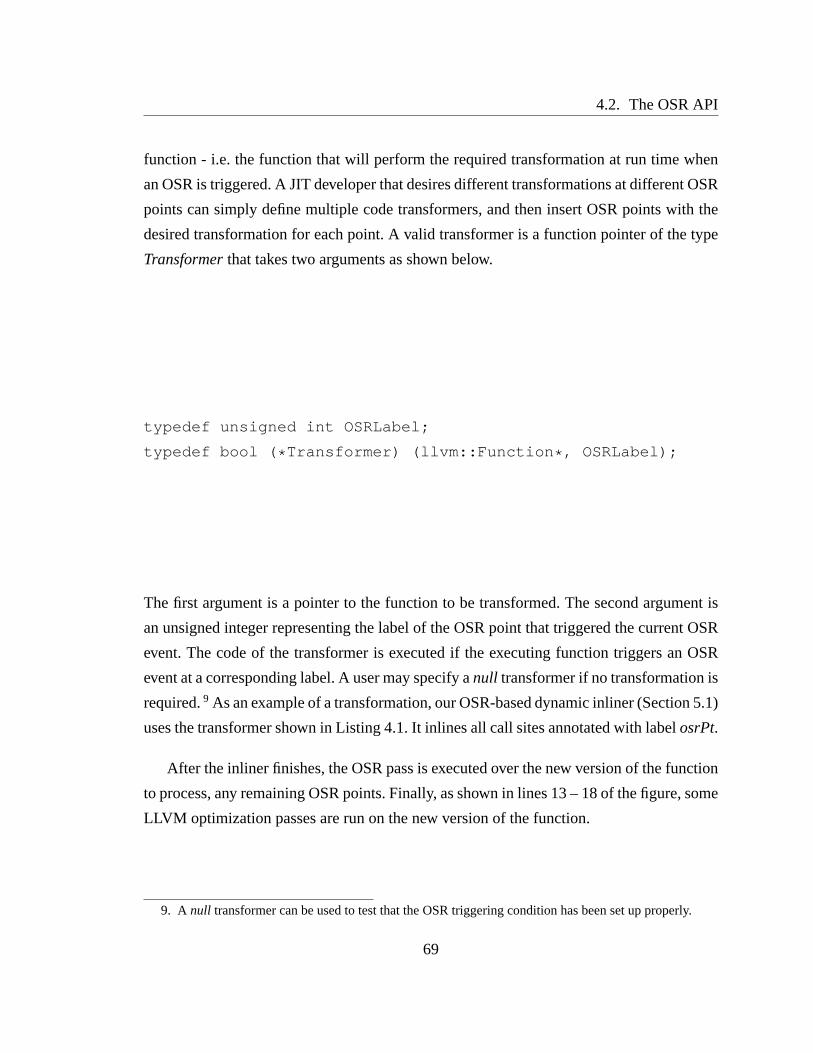
4.2. The OSR API
function - i.e. the function that will perform the required transformation at run time when
an OSR is triggered. A JIT developer that desires different transformations at different OSR
points can simply define multiple code transformers, and then insert OSR points with the
desired transformation for each point. A valid transformeris a function pointer of the type
Transformerthat takes two arguments as shown below.
typedef unsigned int OSRLabel;
typedef bool ( * Transformer) (llvm::Function * , OSRLabel);
The first argument is a pointer to the function to be transformed. The second argument is
an unsigned integer representing the label of the OSR point that triggered the current OSR
event. The code of the transformer is executed if the executing function triggers an OSR
event at a corresponding label. A user may specify anull transformer if no transformation is
required.9 As an example of a transformation, our OSR-based dynamic inliner (Section 5.1)
uses the transformer shown in Listing 4.1. It inlines all call sites annotated with labelosrPt.
After the inliner finishes, the OSR pass is executed over the new version of the function
to process, any remaining OSR points. Finally, as shown in lines 13 – 18 of the figure, some
LLVM optimization passes are run on the new version of the function.
9. A null transformer can be used to test that the OSR triggering condition has been set up properly.
69

A Modular Approach to On-Stack Replacement in LLVM
Listing 4.1 – A code transformer.1 bool inlineAnnotatedCallSites (llvm :: Function*F, osr :: OSRLabel osrPt){2 ...3 llvm :: McJITInliner inliner (FIM, osrPt , TD);4 inliner .addFunction( inlineVersion );5 inliner . inlineFunctions ();6 ...7 // create and run the OSR Pass8 llvm :: FunctionPassManager FPM(M);9 FPM.add(createOSRInfoPass());
10 FPM.run(*runningVersion);11
12 // create and run LLVM optimization passes13 llvm :: FunctionPassManager OP(M);14 OP.add(llvm:: createCFGSimplificationPass ());15 OP.add(llvm:: ConstantPropagationPass ());16 ...17 OP.run(* runningVersion ); ...18 }
To illustrate with a concrete example of inserting OSR points, our OSR-based dynamic
inlining implementation uses the code snippet shown in Listing 4.2 to insert conditional
OSR points after generating the loop header block containing only φ nodes. In the code
snippet (lines 6 – 12), a new basic blockosr is created and the call togenOSRSignalinserts
an OSR point into the block. The rest of the code inserts a conditional branch instruction
into targetand completes the generation of the LLVM IR for the loop.
70

4.2. The OSR API
Listing 4.2 – Sample code for inserting an OSR point.1
2 ...3 // get the loop header block−−− the target4 llvm :: BasicBlock* target = builder . GetInsertBlock ();5 llvm :: Function* F = target−>getParent();6 // create the osr instruction block7 llvm :: BasicBlock* osrBB =8 llvm :: BasicBlock :: Create(F−>getContext(),"osr" , F);9 // now create an osr pt and register a transformer
10 llvm :: Instruction* marker =11 osr :: Osr ::genOSRSignal(osrBB,12 inlineAnnotatedCallSites ,13 loopInitializationBB );14 ...15 // create the osr condition instruction16 llvm :: Value *osrCond = builder .CreateICmpUGT(counter,17 getThreshold( context ),"ocond" );18 builder .CreateCondBr(osrCond, osrBB, fallThru );19 ...
4.2.2 Adding the OSR Transformation Pass
After modifying the JIT with the capability to insert OSR points, the next step is to add
the creation and running of the OSR transformation pass. Whenthe OSR pass is run on a
function with OSR points, the pass automatically instruments the function by adding the
OSR machinery code at all the OSR points (note that the JIT-compiler developer only has
to invoke the OSR pass, the pass itself is provided by our OSR module).
The OSR pass is derived from the LLVM function pass. Listing 4.3 shows a simplified
interface of the pass. An LLVM front-end, that is, an LLVM code generator, can use the
following code snippet to create and run the OSR pass on a function F after the original
LLVM optimizer in Figure 4.2(b) finishes.
llvm::FunctionPass * OIP = osr::createOSRInfoPass();
OIP->runOnFunction( * F);
The OSR pass can also be added to an LLVM function pass manager.
71

A Modular Approach to On-Stack Replacement in LLVM
Listing 4.3 – The OSR Pass interface.
namespace osr{class OSRInfoPass : public llvm :: FunctionPass{public :
OSRInfoPass();virtual bool runOnFunction(llvm::Function& F);virtual const char* getPassName() const{ return ”OSR Info Collection Pass”;} ...};llvm :: FunctionPass* createOSRInfoPass ();}
4.2.3 Initialization and Finalization
To configure the OSR subsystem during the JIT’s start-up time, the JIT developer must
add a call to the methodOsr :: init . This method initializes the data structures and registers
the functions used later by the OSR subsystem. The JIT developer must also add a call to the
methodvoid Osr:releaseMemory()to de-allocate the memory allocated by the OSR system.
The code snippet in Listing 4.4 shows how an existing JIT can initialize and release the
memory used by the OSR subsystem. As shown in line 4, the arguments toOsr :: init are
a JIT execution engine and the module. The execution engine and the module are used to
register the functions used by the system.
Listing 4.4 – Initialization and Finalization in the JIT’smainfunction.int main(int argc , const char** argv) {
...// initialize the OSR data structures ...Osr :: init (EE, module);
... // JIT ' s Code
// free up the memory used for OSR ...Osr :: releaseMemory();...
return 0;}
72
4.3. Implementation
4.3 Implementation
In the previous section, we outlined our API which provides asimple and modular ap-
proach to adding OSR support to LLVM-based JIT compilers. Inthis section, we present
our implementation of the API. Our implementation assumes that the application is single-
threaded. We first discuss the main challenges that influenced our implementation deci-
sions, and our solution to those challenges.
4.3.1 Implementation Challenges
Our first challenge was how to mark OSR points. Ideally, we needed an instruction to
represent an OSR point in a function. However, adding a new instruction to LLVM is a non-
trivial process and requires rebuilding the entire LLVM system. It will also require users of
our OSR module to recompile their existing LLVM installations. Hence, we decided to use
the existing call instruction to mark an OSR point. This alsogives us some flexibility as the
signature of the called function can change without the needto rebuild any LLVM library.
A related challenge was to identify at which program points OSR instructions should
be allowed. We decided that the beginning of loop bodies wereideal points because we
could ensure that the control flow and phi-nodes in the IR could be correctly patched in a
way that does not disrupt other optimization phases in LLVM.
The next issue that we considered was portability. We decided to implement at the
LLVM IR, rather than at a lower level, for portability. This issimilar to the approach used
in Jikes research VM [FQ03], which uses byte-code, rather than machine code to represent
the transformed code. This approach also fits well with the extensible LLVM pass manager
framework.
A very LLVM-specific challenge was to ensure that the code of the new version is
accessible at the old address without recompiling all the callers of the function. Finding a
solution to this was really a key point in getting an efficientand local solution.
Finally, when performing an OSR, we need to save the current state (i.e., the set of
live values) of an executing function and restore the same state later. Thus, the challenge is
73

A Modular Approach to On-Stack Replacement in LLVM
how to restore values while at the same time keeping the SSA-form CFG of the function
consistent.
We now explain our approach which addresses all these challenges. In particular, we
describe the implementation ofInserterandOSR Passshown in Figure 4.2(b).
4.3.2 OSR Point
In Section 4.2.1, we explained how a developer can add the capability to insert OSR
points to an existing JIT. Here we describe the representation of OSR points.
We represent an OSR point with a call to a native function named @ osrSignal. It
has the following signature.
declare void @__osrSignal( i8* , i64)
The first formal parameter is a pointer to some memory location. A corresponding ar-
gument is a pointer to the function containing the call instruction. This is used to simplify
the integration of inlining; we discuss this in detail in Section 4.3.5. The second formal
parameter is an unsigned integer. A function may have multiple OSR points; the integer
uniquely identifies an OSR point.
The OSR module maintains a table named OSR function table (oft). The table maps a
function in LLVM IR onto a set of OSR-point entries. The set cangrow or shrink dynam-
ically as new OSR points are added (e.g., after a dynamic inlining) and old OSR points
removed (e.g., after an OSR). An entrye in the set is an ordered pair.
e = (osr call inst, code transformer)
The first member of the pair —osr call inst — is the call instruction that marks the posi-
tion of an OSR point in a basic block. The second is thecode transformer(Section 4.2.1).
4.3.3 The OSR Pass
The OSR pass in Figure 4.2(b) is a key component of our OSR implementation. As
shown in Listing 4.3, the OSR transformation pass is derivedfrom the LLVM FunctionPass
type. Like all LLVM function passes, the OSR pass runs on a function via itsrunOnFunc-
tion (Listing 4.3) method.
74

4.3. Implementation
The pass first inspects a function’soft entry to determine whether the function has at
least one OSR point. It returns immediately if the function has no OSR points. Otherwise,
it instruments the function at each OSR point. Figure 4.3 shows a simplified CFG of a loop
with no OSR points. The basic block labelledLH1 is the loop header.LB contains the code
for the body of the loop; and the loop exits atLE.
ENTRY:...
LH1:...
br i1 %loopCond,label %LB, label %LE
LE:...
LB:...
br label %LH1
false true
Figure 4.3 – A CFG of a loop with no OSR points.
Figure 4.4 shows a simplified CFG for the loop in Figure 4.3 withan OSR point. This
represents typical code an LLVM front-end will generate with OSR enabled. Insertion of
OSR points is performed byInsertershown in Figure 4.2(b). The loop header block (now
LH0 in the Figure 4.4) terminates with a conditional branch instruction that evaluates the
Boolean flag%osrCondand branches to either the basic block labelledOSRor to LH1.
LH1 contains the loop termination condition instruction.LB contains the code for the body
of the loop; the loop exits atLE.
The OSR compilation pass performs a liveness analysis on theSSA-form CFG to deter-
mine the set of live variables at a loop header such asLH0 in Figure 4.4. It creates, using the
LLVM cloning support, a copy of the function named thecontrol version. As we explain
later in this section, this is used to support the transitionfrom one version of the function
75

A Modular Approach to On-Stack Replacement in LLVM
ENTRY:...
LH0:...
br i1 %osrCond,label %OSR, label %LH1
OSR:
call void @ osrSignal(...)
br label %LH1
LH1:...
br i1 %loopCond,label %LB, label %LE
LE:...
LB:...
br label %LH0
truefalse
false true
Figure 4.4 – The CFG of the loop in Figure 4.3 after inserting anOSR point.
to another at run time. It also creates a descriptor [HCU92, FQ03] for the function. The
descriptor contains useful information for reconstructing the state of a function during an
OSR event. In our approach, a descriptor is composed of:
– a pointer to the current version of the function;
– a pointer to the control version of the function;
– a map of variables from the original version of the functiononto those in the control
version; and
– the sets of the live variables collected at all OSR points.
After running the OSR pass on the loop shown in Figure 4.4, theCFG will be trans-
formed into that shown in Figure 4.5. Notice that in the transformed CFG, the OSR block
now contains the code to save the runtime values of the live variables and terminates with a
return statement. We now describe in detail the kinds of instrumentation added to an OSR
block.
76

4.3. Implementation
ENTRY:...
LH0:...
br i1 %osrCond,label %OSR, label %LH1
OSR:
call void @ osrSignal(...)
store ......
ret ...
LH1:...
br i1 %loopCond,label %LB, label %LE
LE:...
LB:...
br label %LH0
truefalse
false true
Figure 4.5 – The transformed CFG of the loop in Figure 4.4 afterrunning the OSR Pass.
4.3.3.1 Saving Live Values
To ensure that an executing function remains in a consistentstate after a transition
from the running version to a new version, we must save the current state of the executing
function. This means that we need to determine the live variables at all OSR points where
an OSR transition may be triggered. Dead variables are not useful.
As highlighted in Section 4.2, we require that the header of aloop with an OSR point
always terminates with a conditional branch instruction ofthe form:
br i1 %et, label %osr, label %cont
This instruction tests whether the function should performOSR. If the test succeeds (i.e.,
%et is set totrue), the succeeding block beginning at label%osrwill be executed and OSR
transition will begin. However, if the test fails, execution will continue at the continuation
block,%cont. This is the normal execution path.
77

A Modular Approach to On-Stack Replacement in LLVM
In %osrblock, we generate instructions for saving the runtime value of each live vari-
able computed by the liveness analysis. The code snippet in Listing 4.5 shows a typicalosr
block in a simplified form.
Listing 4.5 – OSR instrumentation.1
2 osr :3 call void @ osrSignal(f, i64 1)4 store double%7, double* @live5 store double%8, double* @live16 ...7 store i32 1, i32* @osr flag8 call void @ recompile(f, i32 1)9 call void @f (...)
10 call void @ recompileOpt(f)11 ret void
The call to@ osrSignal(f, i64 1)in line 2 marks the beginning of the block. Fol-
lowing this call is a sequence ofstore instructions. Each instruction in the sequence saves
the runtime value of a live variable into a global variable@live*. The laststore instruction
stores the value 1 into@osr flag. If @osr flag is non-zero at run time, then the executing
function is performing an OSR transition. We explain the functions of the instructions in
lines 7 – 10 later.
The saved variables are mapped onto the variables in the control version. This is a key
step as it allows us to correctly restore the state of the executing function during an OSR.
4.3.4 Restoration of State and Recompilation
The protocol used to signify that a function is transitioning from the executing version
to a new version, typically, a more optimized version10, is to set a global flag. The flag is
reset after the transition.
At run time, the running function executes the code to save its current state. It then
calls the compiler to recompile itself and, if a codetransformeris present, the function is
10. It may also transition from an optimized version to a lessoptimized version depending on the applica-
tion.
78

4.3. Implementation
transformed before recompilation. The compiler retrievesthe descriptor of the function and
updates the running version using thecontrolversion as illustrated in Figure 4.6.
fo
fc
fo
fc
CT :fc = clone(fo)OT :
move(fc, fo)
Figure 4.6 – State management cycle.
Let fo denote the original version of the LLVM IR of the running function, andfc
denote the control version that was generated by cloning theoriginal version. We denote
the set of all the live variables offo at the program pointpo with Vo(po). Similarly,Vc(pc)
denotes the state of the control version at the matching program pointpc. Becausefc is a
copy offo, it follows that
Vo(po) ≡ Vc(pc).
Figure 4.6 illustrates the state management cycle of the running function. The function
starts with versionfo. At compilation time11 (shown as eventCT in Figure 4.6), we clone
fo to obtainfc. We then compilefo. At run time, when an OSR (eventOT in Figure 4.6) is
triggered by the running function, we first remove the instructions info and thenmovethe
code (LLVM IR) of fc into fo, transform/optimize as indicated by the OSR transform, and
then recompilefo and execute the machine code offo.
This technique ensures that the machine code of the running function is always accessi-
ble at the same address. Hence, there is no need to recompile its callers: the machine code
of the transformedfo is immediately available to them at the old entry point of therunning
function.
To locate the continuation program pointpo (po ≡ pc), the compiler recovers the OSR
entry of the current OSR identifier; using the variable mappings in the descriptor, finds the
instruction that corresponds to the current OSR point. Fromthis, it determines the basic
11. This includes the original compilation and all subsequent recompilations due to OSR.
79

A Modular Approach to On-Stack Replacement in LLVM
block of the instruction. Because the basic block of an OSR point instruction has one and
only one predecessor, the compiler determines the requiredtarget,po.
4.3.4.1 Restoration of State
To restore the state of the executing function, we create a new basic block namedprolog
and generate instructions to load all the saved values in this block; we then create another
basic block that merges a new variable defined in theprologwith that entering the loop via
the loop’s entry edge. We ensure that a loop header has only two predecessors and because
LLVM IR is in SSA form, the new block consists ofφ nodes with two incoming edges: one
from the initial loop’s entry edge and the other fromprolog. Theφ nodes defined in the
merger block are used to update the users of an instruction that corresponds to a saved live
variable in the previous version of the function.
Figure 4.7 shows a typical CFG of a running function before inserting the code for
recovering the state of the function. The basic blockLH1 defines aφ node for an induction
variable (%i in Figure 4.7) of a loop in the function. The body of the loop,LB, contains a
add instruction that increments the value of%i by 1.
Assuming that we are recovering the value of%i from the global variable@live i,
Figure 4.8 shows the CFG after inserting the blocks for restoring the runtime value of%i.
In this figure,prolog contains the instruction that will load the runtime value of%i from
the global variable@live i into % i; similarly, the basic blockprolog.exitcontains aφ
instruction (% m i) that merges% i from prolog and the value 1 fromENTRY. This
variable (i.e.,% m i) replaces the incoming value (1) fromENTRYin the definition of
%i in the loop header (LH1) as shown in Figure 4.8. Notice that the incoming blockENTRY
has been replaced withprolog.exit(PE) in the definition of%i in LH1.
Fixing the CFG to keep the SSA form consistent is non-trivial.A simple replacement of
a variable with a new variable does not work. Only variables dominated by the definitions
in the merger block need to be replaced. Newφ nodes might be needed at some nodes with
multiple incoming edges (i.e., only those that are in the dominance frontier of the merger
block). Fortunately, the LLVM framework provides an SSA Updater that can be used to
update the SSA-form CFG. We exploited the SSA Updater to fix theCFG.
80

4.3. Implementation
ENTRY:...
LH1:
%i = phi i64[1, %Entry], [%i.u, %LB]
...br i1 %loopCond,
label %LB, label %LE
LE:...
LB:...
%i.u = add i64 %i, 1...
br label %LH1
falsetrue
Figure 4.7 – A CFG of a loop of a running function before inserting the blocks for state
recovery.
81

A Modular Approach to On-Stack Replacement in LLVM
prolog.entry:...
br i1 %ocond,label %ENTRY, label %prolog
prolog:
% i = load i64* @live i...
br label %prolog.exit
ENTRY:...
LH1:
%i = phi i64[% m i, %PE], [%i.u, %LB]
...br i1 %loopCond,
label %LB, label %LE
LE:...
prolog.exit(PE):
% m i = phi i64
[1, %Entry], [% i, %prolog]...
br label %LH1
LB:...
%i.u = add i64 %i, 1...
br label %LH1
falsetrue
Figure 4.8 – The CFG of the loop represented by Figure 4.7 afterinserting the state recovery
blocks.
82

4.3. Implementation
To complete the state restoration process, we must fix the control flow to ensure that
the function continues at the correct program point. For this, we insert a new entry block
namedprolog.entrythat loads@osr flag and tests the loaded value for zero to determine,
during execution, whether the function is completing an osrtransition or its being called
following a recent completion of an OSR. The content of the newentry block is shown in
the following code snippet.
1 prolog . entry :2 %osrPt = load i32* @osr flag3 %cond = icmp eq i32%osrPt, 04 br i1 %cond, label %entry , label %prolog
If %osrP t is non-zero, the test succeeds and the function is completing an OSR; it will
branch to%prolog. In %prolog, all the live values will be restored and control will pass
to the target block: the loop header where execution will continue. However, if%osrP t is
zero, the function is not currently making a transition: it is being called anew. It will branch
to the original entry basic block, where its execution will continue.
As shown in Figure 4.8, the basic blockprolog.entry terminates with a conditional
branch instruction. The new version of the running functionwill begin its execution from
prolog.entry. After executing the block, it will continue at eitherprolog or ENTRY(the
original entry block of the function) depending on the runtime value of%cond.
4.3.4.2 Recompilation
We now return to the instructions in lines 7 – 10 of Listing 4.5. The instruction in line
7 calls the compiler to perform OSR and recompilef using the code transformer attached
to OSR point 1. After that, functionf will call itself (as shown in line 8), but this will
execute the machine code generated for its new version. Thisworks because the LLVM
recompilation subsystem replaces the instruction at the entry point of functionf with a
jump to the entry point of the new version. During this call, the function completes OSR
and resumes execution. The original call will eventually return to the caller any return value
returned by the recursive call.
83

A Modular Approach to On-Stack Replacement in LLVM
Normally after an OSR, subsequent calls (if any) off executes the code in thepro-
log.entry, which tests whether or not the function is currently performing an OSR. How-
ever, this test succeeds only during an OSR transition; in other words, the execution of
the code inprolog.entryafter an OSR has been completed is redundant. To optimize away
theprolog.entry, we again call the compiler (line 9 in Listing 4.5) but this time, the com-
piler only removes theprolog.entryand consequently, other dead blocks, and recompilef .
In Section 5.3.2, we compare the performance of our benchmarks when theprolog.entry
is eliminated with the performance of the same benchmarks when theprolog.entryis not
eliminated.
4.3.5 Inlining Support
Earlier, we discussed the implementation of OSR points and how the OSR transforma-
tion pass handles OSR points. However, we did not specify howwe handled OSR points
inserted into a function from an inlined call site. A seamless integration of inlining opti-
mization poses further challenges. When an OSR event is triggered at run time, the runtime
system must retrieve the code transformer attached to the OSR point from theoft entry of
the running function. How then does the system know the original function that defined an
inlined OSR point? Here we explain how our approach handles inlining.
Remember that an OSR point instruction is a call to a function.The first argument is
a pointer to the enclosing function. Therefore, when an OSR point is inlined from another
function, the first argument to the inlined OSR point (i.e., acall instruction) is a function
pointer to the inlined function. From this, we can recover the transformerassociated with
this point by inspectingoft using this pointer. We can then modify these OSR points by
changing the first argument into a pointer to the current function and assign a new ID to
each inlined OSR point. We must also update theoft entry of the caller to reflect these
changes.
We distinguish two inlining strategies: static and dynamic. In static inlining, a call site
is expanded before executing thecaller. This expansion may introduce a new OSR point
from the callee into the caller and invalidates all the state information collected for the
existing OSR points. We regenerate this information after any inlining process.
84

4.4. Summary
Dynamic inlining concerns inlining of call sites in a running function during the exe-
cution of the function after observing, for some time, its runtime behaviour. Typically, we
profile a program to determinehotcall sites and inline those subject to some heuristics. We
used OSR support to implement dynamic inlining of call sitesin long-running loops. We
discuss this implementation in the next chapter.
4.4 Summary
In this chapter, we have introduced a modular approach to implementing OSR for
LLVM-based JIT compilers. Our approach should be very easy for others to adopt because
it is based on the LLVM and is implemented as an LLVM pass. Furthermore, we found
a solution which does not require any special data structures for storing stack frame val-
ues, nor any instrumentation in the callers of functions containing OSR points. It also does
not introduce any changes to LLVM which would require rebuilding the LLVM system.
Finally, our approach also provides a solution for the case where a function body contain-
ing OSR points is inlined, in a way that maintains the OSR points and adapts them to the
inlined context.
In the next chapter, we describe a case study of how we have used our OSR imple-
mentation to support selective dynamic inlining of hot callsites in long-running loops in
the McVM JIT compiler for the MATLAB language. Then we describe and discuss the ex-
periments that we conducted to measure the overheads OSR andthe benefits of our OSR-
supported selective dynamic inlining.
85

A Modular Approach to On-Stack Replacement in LLVM
86

Chapter 5
Selective Dynamic Inlining in McVM
This chapter is a continuation of the previous chapter, which is about the implementa-
tion of our OSR approach. Here, we present an example application of the OSR approach
to support selective dynamic inlining in McJIT. We selectedthis as our first application of
OSR because inlining impacts OSR since it must properly dealwith OSR points in the in-
lined functions. Moreover, inlining can provide larger scope for many traditional compiler
optimizations and can increase the opportunity for loop vectorization.
The main contributions of this chapter are
Using OSR in McJIT for selective dynamic inlining: In order to demonstrate the effec-
tiveness of our OSR module, we have implemented an OSR-based dynamic inliner
that will inline function calls within dynamically hot loopbodies. This has been com-
pletely implemented in McVM/McJIT.
Experimental measurements of overheads/benefits:We have performed a variety of
measurements on a set of 16 MATLAB benchmarks. We have measured the over-
heads of OSRs and selective dynamic inlining. This shows thatthe overheads are
usually acceptable and that dynamic inlining can result in performance improve-
ments.
87

Selective Dynamic Inlining in McVM
5.1 The McJIT dynamic inliner
In our approach to dynamic inlining, we first modified McJIT toidentify potential in-
lining candidates. In our case, a call is considered an inlining candidate if the body of the
called function is less than 20 basic blocks, or it is less than 50 basic blocks and it has
an interpreter environment associated with the body.1 McJIT generates LLVM IR for each
function in a program. The LLVM IR generated by McJIT may contain calls to the inter-
preter for special cases and for those cases the symbol environment set-up code facilitates
the interaction with the interpreter. In our case, inliningcan reduce the interpreter environ-
ment overheads.
We then modified McJIT so that loops which contain potential inlining candidates are
instrumented with a hotness counter and a conditional whichcontains an OSR point (where
the OSR point is associated with a new McJIT inlining transformer). When an OSR triggers
(i.e. the hotness counter reaches a threshold), the McJIT inlining transformation will inline
all potential inlining candidates associated with that OSRpoint.
There are many strategies for determining which loops should be given an OSR point,
and a JIT developer can define any strategy that is suitable for his/her situation. For McJIT,
we defined two such general strategies, as follows:
CLOSEST Strategy: The LLVM front-end is expected to insert OSR points only in the
loop that is closest to the region that is being considered for optimization. For ex-
ample, to implement a dynamic inlining optimization using this strategy, an OSR
point is inserted at the beginning of the closest loop enclosing an interesting call site.
This strategy is useful for triggering an OSR as early as possible, i.e., as soon as that
closest enclosing loop becomes hot.
OUTER Strategy: The LLVM front-end is expected to insert an OSR point at the be-
ginning of the body of the outer-most loop of a loop nest containing the region of
interest. This approach is particularly useful for triggering many optimizations in a
loop nest with a single OSR event. In the case of dynamic inlining, one OSR will trig-
ger inlining of all inlining candidates within the loop nest. The potential drawback
1. We experimented with different thresholds for basic blocks but found 20 and 50 to work best for our
benchmarks.
88

5.1. The McJIT dynamic inliner
of this strategy is that the OSR will not trigger until the outermost loop becomes hot,
thus potentially delaying an optimization.
In Figure 5.1, we illustrate the difference between the two strategies using an hypothet-
ical loop nest. We use a call site to represent an interestingregion for optimization.
L0
L1
C2: call f()
L2
C3: call g()
L3
C0: call h()
(a) A four-loop loop nest
L0
OSR Point 1:L1
C2: call f()
L2
C3: call g()
L3
C0: call h()
(b) Outer-most-loops Strategy
L0
OSR Point 1:L1
C2: call f()
OSR Point 2:
L2
C3: call g()
OSR Point 3:
L3
C0: call h()
(c) Closest-loops Strategy
Figure 5.1 – A loop nest showing the placement of OSR points using the closest or outer-
most strategy.
A loop is represented with a box. The box labelledL0 denotes the outer-most loop of
the loop nest. The nest contains four loops and has a depth of 3. LoopsL1 andL3 are at the
same nesting level.L2 is nested insideL1. The loop nest has three call sites:C0 in loopL0,
C2 in loopL2, andC3 in loopL3. Figure 5.1(a) shows the loop nest with no OSR points.
With the outer-most-loops strategy, an OSR point will be inserted only at the beginning
of the outer-most loop,L0 as shown in Figure 5.1(b). However, if the strategy is closest-
enclosing loops, the front-end will insert an OSR point at the beginning of loopsL0, L2,
andL3 as shown in Figure 5.1(c). AlthoughC2 is insideL1, no OSR points are inserted
intoL1 becauseL1 is not the closest-enclosing loop ofC2.
As shown in the figure, the outer-most-loops strategy causesonly one OSR point to be
inserted into the entire loop nest, while the closest-enclosing-loops strategy causes three
89

Selective Dynamic Inlining in McVM
OSR points to be inserted. Thus, depending on the optimization performed during an OSR
event, the choice of strategy can make a difference in performance.
In our VM, a user specifies an OSR strategy from the command line when invoking the
VM, like the following example.
./mcvm -jit_enable true -jit_osr_enable true
-jit_osr_strategy outer.
This command starts McVM with OSR enabled withouterstrategy. In our JIT, the default
strategy isouter.
When the OSR triggers it calls the McJIT inliner transformation. Our McJIT inliner
calls the LLVM basic-inliner library to do the actual inlining. However, the McJIT inliner
must also do some extra work because it must inline the correct version ofcalleefunction
body. The key point is that if thecalleehas an OSR point, it must not inline the version
of the callee which has already been instrumented with the code to store values of the live
variables at this OSR point. If this version is inlined into thecaller — the function that is
performing OSR— the instrumentation becomes invalid as the code does not correctly save
the state of the caller at that inlined OSR point. We resolvedthis problem by recovering the
control version of the called function (callee) and modifying the call site. We change the
function called by the call instruction to the control version of the callee. For instance, if
the inlined call site iscall void @f(...) , and the control version off is f ′, then the
call site will be changed tocall void @f'(...) . Note that the control version has an
identical OSR point but is not instrumented to save the runtime values of live variables at
that program point. For consistency, the function descriptor of the function is updated after
inlining as outlined in Section 4.3.5.
5.2 Symbol Environment Simplification
One important optimization that we perform on an inlined code region is the symbol
environment optimization. As discussed in Section 2.2.3, the code of a function can contain
calls to the interpreter. Some calls to the interpreter require the function’s symbol environ-
ment, and a function that contains such calls has symbol environment initialization code in
90

5.2. Symbol Environment Simplification
its entry basic block. If a function with a symbol environment is frequently called within a
hot loop body, the execution of the symbol environment set-up code can be a major source
of overhead, especially if multiple functions with symbol set-up code have been inlined
into a function.
Inlining, however, enables an opportunity to eliminate thesymbol set-up code from an
inlined code region. If the calling function has a symbol environment set-up in its entry
block, this symbol environment can be used by the code in the inlined region. This will
render the symbol set-up code from an inlined function redundant. The code can then be
removed from the inlined region.
As an example, Listing 5.1 shows the inner loop of thesim anl [mat13] MATLAB
program.
Listing 5.1 – The inner loop ofsim anl.1 for k=0:5002 %We generate new test point using muinv function [3]3 dx=mu inv(2* rand(size(x))−1,mu).* (u−l);4 x1=x+dx;5 x1=(x1< l ).* l+(l ≤ x1 ).* ( x1 ≤ u).* x1+(u< x1).*u;6 fx1=feval( f ,x1);df=fx1−fx;7
8 if (df < 0 || rand < exp(−T*df/(abs(fx)+eps)/TolFun))==19 x=x1;fx=fx1;
10 end11
12 if fx1 < f0 ==113 x0=x1;f0=fx1;14 end15 end
The entry basic block of the LLVM code generated by McJIT forsim anl contains the
instructions shown in Listing 5.2. Instructions 5 and 7 set up a symbol environment for
functionsim anl.
91

Selective Dynamic Inlining in McVM
Listing 5.2 – LLVM code forsim anl entry basic block. (We show only
the most relevant instructions.)1 define void @sim anl 0x1f86a80({ i8* , i8* , i8* , i8* , i64 , double, i64}* %arg ,2 { i8 * , i8* , i64 }* %arg1) {3 entry :4 ...5 %tmp13 = call i8* @''ProgFunction::getLocalEnv''6 ( i8* inttoptr ( i64 30596480to i8 * ))7 %env = call i8* @''Environment::extend'' (i8* %tmp13)8 ...
Line 3 of Listing 5.1 contains a call to functionmu inv. The MATLAB code, and the
corresponding LLVM code generated by McJIT formu inv is shown in Listing 5.3 and
Listing 5.4 respectively.
Listing 5.3 – Functionmu inv.1 function x=mu inv(y,mu)2 %This function is used to generate new point according to lower and3 %upper %and a random factor proportional to current point .4 x=(((1+mu). abs(y)−1)/mu).*sign(y );5 end
92

5.2. Symbol Environment Simplification
Listing 5.4 – McJIT generated LLVM code formu inv.1 define void @mu inv 0x1f869a0({ i8* , double, i64}* %arg , { i8* , i64 }* %arg1) {2 entry :3 ...4 %tmp5 = call i8* @''ProgFunction::getLocalEnv''5 ( i8* inttoptr ( i64 30596288to i8 * ))6 %r env= call i8* @''Environment::extend'' (i8* %tmp5 )7 ...8 br i1 %tmp11, label%bb29, label%bb9 bb: ; preds =%entry
10 %tmp12 = call i8* @''ArrayObj::getArrayObj'' (i8* %tmp9 , i64 0)11 %tmp13 = call i8* @''Environment::bind'' (i8* %r env,12 i8* inttoptr ( i64 30559968to i8 * ), i8* %tmp12)13
14 %tmp14 = call i8* @''MatrixF64Obj::makeScalar'' (double%tmp7 )15 %tmp15 = call i8* @''Environment::bind'' (i8* %r env,16 i8* inttoptr ( i64 30560032to i8 * ), i8* %tmp14)17
18 %tmp16 = call i8* @''Interpreter::evalBinaryExpr''19 ( i8* inttoptr ( i64 33888032to i8 * ), i8* %r env)20 ...21 ...22 }
Notice that the LLVM code for functionmu inv (Listing 5.4) contains a symbol en-
vironment set-up code in lines 4 – 6; some uses of the symbol environment (i.e., LLVM
virtual register%r env created in line 6) for runtime variable binding in lines 11 and 15,
and for evaluating an expression in line 18 – 19.
If our dynamic inliner decides to inline functionmu inv into functionsim anl, the inner
loop of sim anl shown in Listing 5.1 will contain the set up code and will be executed
many times. Because functionsim anl also has a symbol environment associated with it
(i.e.,%env defined in Listing 5.2), it is possible to eliminate the symbol set up instructions
in the inlined region corresponding to the code ofmu inv.
Thus, we use the algorithm in Algorithm 1 to eliminate symbolenvironment set-up
code from an inlined region. The input to Algorithm 1 is a function in LLVM IR whose
relevant call sites have just been inlined, and a set of basicblocks. Each basic block in the
set is the beginning of an inlined region (the code of the called function at an inlined call
site).
93

Selective Dynamic Inlining in McVM
Input : LLVM IR, and a set of LLVM basic blocks
Output : A simplified LLVM IR
if caller has a symbol environmentE then/* process each inlined region */
for each inlined regionR do
if R has a symbol environmentER then
find all the uses ofER in R ;
for each useU of ER do
replaceER with E;
end
remove the definition ofER fromR
end
end
end
Algorithm 1: Simplification of symbol environments.
The algorithm first checks whether there are inlined regionsand searches the entry
basic block of the input function (which we call thecaller) to find the symbol environment
associated with the function. If no symbol environment is found in the entry block, the
algorithm terminates. If, however, the environment is found, the algorithm processes each
code region found in the input set of basic blocks. It locatesthe symbol environment in the
current code region and replaces all the uses of the symbol environment found in the region
with the symbol environment of the caller. It then removes the set up code for the symbol
environment in the code region.
In the next section, we discuss our experimental results, and the impact of this symbol
environment simplification on performance.
5.3 Experimental Results
We used our McJIT dynamic inliner to study the overheads of OSR and the potential
performance benefit of inlining. We used a collection of MATLAB benchmarks from a
94

5.3. Experimental Results
previous MATLAB research project and other sources [RGG+96, Cle04, Pre86], Table 5.1
gives a short description of each benchmark. All the benchmarks have one or more loops,
the table also lists the total number of loops and max loop depth for each benchmark.
BM Description # Loops Max Depth
adpt adaptive quadrature using Simpson’s rule 4 2
capr capacitance of a transmission line using finite 10 2
difference and and Gauss-Seidel iteration.
clos transitive closure of a directed graph 4 2
crni Crank-Nicholson solution to the one 7 2
dimensional heat equation
dich Dirichlet solution to Laplace’s equation 6 3
diff Young’s two-slit diffraction experiment 13 4
edit computes the edit distance of two strings 7 2
fdtd 3D FDTD of a hexahedral cavity 1 1
with conducting walls
fft fast fourier transform 6 3
fiff finite-difference solution to the wave equation 13 4
mbrt Mandelbrot set 3 2
nb1d N-body problem coded using 1d arrays 6 2
for the displacement vectors
nfrc computes a Newton fractal in the 3 2
complex plane -2..2,-2i..2i
nnet neural network learning AND/OR/XOR functions 11 3
schr solves 2-D Schroedinger equation 1 1
sim Minimizes a function with simulated annealing 2 2
Table 5.1 – The benchmarks.
95

Selective Dynamic Inlining in McVM
The configuration of the computer used for the experimental work is:
Processor: Intel(R) Core(TM) i7-3930K CPU @ 3.20GHz
RAM: 16 GB;
Cache Memory: L1 32KB, L2 256KB, L3 12MB;
Operating System: Ubuntu 12.04 x86-64;
LLVM: version 3.0; and
McJIT: version 1.0.
Our main objectives were:
– To measure the overhead of OSR events on the benchmarks overthe outer-most and
closest-loop strategies. The overhead includes the cost ofinstrumentation and per-
forming OSR transitions. We return to this in Section 5.3.1.
– To measure the impact of selective inlining on the benchmarks. We discuss this in
detail in Section 5.3.2.
We show the results of our experiments in Table 5.2 and Table 5.3. For these experiments,
we collected the execution times (shown ast(s) in the tables) measured in seconds, for 7
runs of each benchmark. To increase the reliability of our data, we discarded the highest
and the lowest values and computed the average of the remaining 5 values. To measure
the variation in the execution times, we computed the standard deviation (STD) (shown as
std) of the 5 values for each benchmark under 3 different categories. All the results shown
in both tables were collected using the outer-most-loops strategy, with the default LLVM
code-generation optimization level.
The column labelledNormalgives the average execution times and the corresponding
STDs of the benchmarks run with OSR disabled, while the column labelledWith OSRgives
similar data when OSR was enabled. ColumnWith OSRin Table 5.3 shows the results
obtained when dynamic inlining plus some optimizations enabled by inlining were on.
The number of OSR points instrumented at JIT compilation time is shown underI of
the column labelled#OSR; while the number of OSR events triggered at run time is shown
under the column labelledT of #OSR. The execution ratio for a benchmark is shown as
the ratio of the average execution time when OSR was enabled to the average execution
96

5.3. Experimental Results
Normal(N) With OSR(O) #OSR Ratio
BM t(s) std t(s) std I T O/N
adpt 17.94 0.06 17.84 0.08 1 1 0.99
capr 11.61 0.01 11.63 0.02 2 2 1.00
clos 16.96 0.01 16.96 0.01 0 0 1.00
crni 7.20 0.04 7.40 0.04 1 1 1.03
dich 13.92 0.01 13.92 0.00 0 0 1.00
diff 12.73 0.07 12.80 0.09 0 0 1.01
edit 6.58 0.03 6.66 0.09 1 0 1.01
fdtd 12.14 0.03 12.16 0.05 0 0 1.00
fft 13.95 0.05 14.05 0.03 1 1 1.01
fiff 8.02 0.01 8.05 0.01 1 1 1.00
mbrt 9.05 0.11 9.22 0.11 1 1 1.02
nb1d 3.44 0.02 3.47 0.01 0 0 1.01
nfrc 9.68 0.05 10.00 0.04 2 2 1.03
nnet 5.41 0.02 5.59 0.03 2 1 1.03
schr 11.40 0.01 11.42 0.03 0 0 1.00
sim 15.26 0.03 15.92 0.07 1 1 1.04
GM 1.01
Table 5.2 – OSR Overhead.
97

Selective Dynamic Inlining in McVM
Normal(N) With OSR(O) #OSR Ratio
BM t(s) std t(s) std I T FI CA O/N
adpt 17.94 0.06 17.85 0.06 1 1 1 F 0.99
capr 11.61 0.01 11.69 0.02 2 2 2 T 1.01
clos 16.96 0.01 17.18 0.22 0 0 0 F 1.01
crni 7.2 0.04 6.73 0.24 1 1 1 T 0.93
dich 13.92 0.01 13.94 0.01 0 0 0 F 1.00
diff 12.73 0.07 12.74 0.04 0 0 0 F 1.00
edit 6.58 0.03 6.66 0.07 1 0 0 F 1.01
fdtd 12.14 0.03 12.13 0.03 0 0 0 F 1.00
fft 13.95 0.05 13.91 0.02 1 1 2 F 1.00
fiff 8.02 0.01 8.26 0.03 1 1 1 F 1.03
mbrt 9.05 0.11 9.06 0.03 1 1 1 F 1.00
nb1d 3.44 0.02 3.47 0.01 0 0 0 F 1.01
nfrc 9.68 0.05 4.26 0.02 2 2 5 T 0.44
nnet 5.41 0.02 5.71 0.03 2 1 1 F 1.05
schr 11.4 0.01 11.45 0.05 0 0 0 F 1.00
sim 15.26 0.03 14.72 0.09 1 1 1 F 0.96
GM 0.95
Table 5.3 – Dynamic inlining using OSR (lower execution ratio is better).
98
5.3. Experimental Results
time when OSR was disabled (this is the default case). ColumnsO/N of Table 5.2 and
O/N of Table 5.3 show, respectively, the ratio for each benchmark when OSR only was
enabled and when OSR and inlining were enabled. The last row of Table 5.2 and Table 5.3
shows the average execution ratio (the geometric mean (GM))over all the benchmarks.
In Table 5.3, we show the number of functions inlined underFI. The column labelled
CA indicates whether at least one function in the benchmark is called again after it has
completed an OSR event.
The STDs of our data sets range from 0.00 to 0.24, showing thatthe execution times
are quite reliable. We now discuss the results of our experiments in detail.
5.3.1 Cost of Code Instrumentation and OSR
Because our approach is based on code instrumentation, we wanted to measure the
overhead of code instrumentation and triggering OSRs. This will allow us to assess the
performance and develop an effective instrumentation strategy.
ColumnO/N of Table 5.2 shows that the overheads range from about 0 to 4%;this is
also the range for the closest-enclosing-loops strategy, suggesting that the overheads under
the two strategies are close. Out of the 16 benchmarks, 10 have at least one OSR point;
and 8 of these 10 benchmarks triggered one or more OSR events.We have not shown the
table of the results for the closest-enclosing loops because out of the 8 benchmarks that
triggered an OSR event, the outer-most and the closest-enclosing loops are different only
in 3 benchmarks:mbrt, nfrc, andsim. The execution ratios for these benchmarks under
the closest-enclosing-loops strategy are: 1.00 formbrt, 1.02 for nfrc, and 1.04 forsim.
The mbrt andnfrc benchmarks have lower execution ratios under the closest-enclosing-
loops strategy. It is not entirely clear whether the closest-enclosing-loops strategy is more
effective than the outer-most-loops strategy; although, with these results, it appears that
using the closest-loops strategy results in lower overheads. The choice between these two
will depend largely on the kinds of the optimizing transformations expected at OSR points.
We return to this discussion in Section 5.3.2, where we examine the effectiveness of our
dynamic inlining optimization.
99

Selective Dynamic Inlining in McVM
We investigated the space performance and found that, depending on the strategy, the
three benchmarks (mbrt, nfrc and sim) compiled up to 3% more instructions under the
closest-enclosing-loops strategy. This is hardly surprising; the OSR overhead depends on
the number of OSR points instrumented and the number of OSR points triggered at run
time. The size of the instrumentation code added at an OSR point in a function depends on
the size of the live variables of the function at that point, and this varies depending on the
position of the OSR point in a loop nest. The outer-most loop is likely to have the smallest
set of live variables.
Although the overhead peaked at 4%, the average overhead over all the benchmarks
(shown asGM in Table 5.2) is 1%. Thus, we conclude that on average, the overhead is rea-
sonable and practical for computation-intensive applications. As we continue to develop
effective optimizations for MATLAB programs, we will work on techniques to use OSR
points in locations where subsequent optimizations are likely to offset this cost and there-
fore increase performance.
5.3.2 Effectiveness of Selective Inlining With OSR
Our objective here is to show that our approach can be used to support dynamic opti-
mization. So, we measured the execution times of the benchmarks when dynamic inlining
is enabled. When an OSR is triggered, we inline call sites in the corresponding loop nest.
ColumnWith OSRof Table 5.3 shows the results of this experiment.
The results show significant improvements forcrni, nfrc andsim. This shows that our
dynamic inlining is particularly effective for this class of programs. Further investigation
revealed that these benchmarks inlined multiple small functions and several of these func-
tions fall back to the McVM’s interpreter to compute some complicated expressions. As
discussed in Section 5.2, McJIT’s interactions with the interpreter are facilitated by setting
up a symbol environment for binding variables at run time. Our dynamic inlining enables
the symbol environment simplfication discussed in Section 5.2, which eliminates the en-
vironment set-up instructions in the inlined code. This is the main cause of performance
improvement innfrc andsim, and is impossible to do without inlining.
100

5.3. Experimental Results
Only thefiff andnnetshow a real decrease in performance when using the outer-most-
loop strategy with inlining. We found that the function inlined bynnetcontains some ex-
pensive cell array operations, which our optimizer is currently unable to handle. The bench-
mark also triggered an OSR event once, but performed three OSR instrumentation phases:
two at the compilation time and one re-instrumentation during the only OSR event.
We wanted to assess the impact of recompilation to optimize the prolog.entryblock
added during an OSR event; so we turned off recompilation after OSR and re-collected the
execution times for the benchmarks. Out of the 9 benchmarks that performed inlining, only
3 benchmarks contain at least one further call to a function that completed an OSR. These
are the rows with the value “T” against the column labelledCA in Table 5.3. The results
for these benchmarks under the no-recompilation after OSR is: 1.01 forcapr, 0.95 forcrni,
and 0.45 fornfrc. These results suggest that the recompilation to remove theprolog.entry
contributes to the increase in performance forcaprandnfrc. The basic block has the poten-
tial to disrupt LLVM optimizations and removing it might lead to better performance. The
recompilation after OSR does not result in a slowdown for theother benchmarks.
In Section 5.3.1, we mentioned that the kinds of the optimizing transformations can
guide the choice of strategy that lead to better performance. Considering the 3 benchmarks
with a loop nest where the outer-most and closest-enclosingloops are different, that is,
mbrt, nfrc and sim, we found that the outer-most-loop strategy outperforms the closest-
enclosing-loop strategy. In particular, thesimbenchmark results in about 5% performance
degradation. These results support our claim.
We recorded the average performance improvement over all the benchmarks (shown
as GM in Table 5.3) of 5%. We conclude that our OSR approach is effective, in that it
efficiently supports this optimization, and that it works smoothly with inlining. To see fur-
ther benefits of OSR for MATLAB, we shall develop more sophisticated optimizations
that leverage the on-the-fly dynamic type and shape information that is very beneficial for
generating better code.
101

Selective Dynamic Inlining in McVM
5.4 Summary
In this chapter, we described how we have used the OSR machinery to implement dy-
namic incremental function inlining. We also described a symbol environment simplifi-
cation optimization. On our benchmarks, we found some performance improvements and
slight degradations, with several benchmarks showing goodperformance improvements.
We used our OSR strategy in the McJIT implementation, and using this implementation,
we demonstrated the feasibility of the approach by measuring the overheads of the OSR
instrumentation for two OSR placement strategies: outer-most loops and closest-enclosing
loops. On our benchmark set, we found overheads of 0 to 4%.
Our ultimate goal is to use OSR to handle recompilation of keyloops, taking advantage
of type knowledge to apply more sophisticated loop optimizations, including parallelizing
optimizations which can leverage GPU and multicores. Thus,as McJIT and MATLAB-
specific optimizations develop, we plan to use OSR to enable such optimizations. In addi-
tion to our own future uses of our OSR implementation, we alsohope that other groups will
also use our OSR approach in LLVM-based JITs for other languages, and we look forward
to seeing their results.
102

Chapter 6
Dynamic Function Evaluation with feval
As we mentioned in Section 1.3.3, MATLAB supports higher-order functions through
the feval construct, which is widely used in many classes of numericalcomputations. A
typical use offeval involves a dynamic evaluation of a function passed in as an argument
to the function whose body contains thefeval call [Mat09a]. For many classes of appli-
cations, such a dynamic evaluation of a fixed function is repeated in a long-running loop,
and is often performed via interpretation.
This chapter focuses on determining iffeval causes significant overheads in both the
interpreter and JIT settings, and then proposes two mechanisms to optimizefeval .
To determine potential overheads offeval , we identified a set of seven benchmarks
that use algorithms that naturally usefeval , and performed initial experiments on three
interpreters (Octave, Mathworks MATLAB 7 in interpreter mode, and McVM in interpreter
mode), plus two JITs (Mathworks MATLAB with the JIT enabled,and McVM with the JIT
enabled).1 These experiments showed, in both the interpreter and JIT situations, that there
are significant overheads for calls viafeval , as compared to direct function calls and
inlined function calls.
To reduce the overheads offeval we then designed and implemented two alternative
mechanisms. The first is the more general of the two mechanisms in that it can handle a
wider variety of uses offeval , and is based on on-the-fly code generation and on-stack
replacement (OSR) techniques implemented in McVM [LH13]. The OSR-based technique
1. Octave is an open source interpreter-only implementation which does not have a JIT.
103

Dynamic Function Evaluation withfeval
identifies potentially importantfeval calls, and then uses McVM’s OSR technology to
specialize thefeval calls to specific direct calls, and to provide correct backupto the
general case when the specialized calls do not match the calling context. We describe the
OSR-based approach in Chapter 7. The second mechanism extendsthe McVM JIT com-
piler with on-the-fly code specialization mechanism to specialize on thevalue of function
parameters in those cases where the parameter is used insidethe body of the function as
the first argument tofeval . This is described in Chapter 8.
This chapter describes our experiments that show significant overheads for calls via
feval for important classes of benchmarks. The discussion here sets the stage for the
descriptions, in Chapter 7 and Chapter 8, of our two mechanismsfor reducing the overheads
of feval calls.
6.1 Motivation and Problem
In this section, we provide some key background on MATLAB andits feval function,
as well our experimental results that demonstrate the significant overheads offeval .
MATLAB and feval
In order to provide some intuition about MATLAB and thefeval challenges, consider
the example MATLAB functionnewtonin Listing 6.1. As shown on line 1, the function
takes four input arguments, with the first argumentfun corresponding to either the name
of a function or a function handle. Note that MATLAB has no declared types, although
the programmer certainly has some expected types in mind, asindicated by the comments
on lines 3 to 13. Indeed, not only does the programmer expect the first argument to be a
string containing the name of a function, but she also expects the named function to take
one input argument and produce two outputs. This is also clear from line 22, wherefeval
is used to call the function provided by the argumentfun. Listing 6.2 shows the definition
of fx3n, which is one possible function that could be provided tonewton.
104

6.1. Motivation and Problem
Listing 6.1 – Newton’s method to find a root of the scalar equation f(x) =
0, adapted from [Rec00a,Rec00b]. Functionfx3nis shown in Listing 6.2.1 function r = newton(fun,x0, xtol , ftol )2
3 % newton Newton's method to find a root of the scalar4 % equation f (x) = 05 % Synopsis: r = newton(fun,x0, xtol , ftol )6 % Input: fun = ( string ) name of mfile that7 % returns f (x) and f '( x ).8 % x0 = initial guess9 % xtol = absolute tolerance on x.
10 % Smallest : xtol=5*eps11 % ftol = absolute tolerance on f (x ).12 % Smallest : ftol =5*eps13 % Output: r = the root of the function14
15 xeps =max(xtol,5*eps);16 feps =max(ftol,5* eps); % Smallest tols are 5*eps17 x = x0; k = 0;18 maxit = 15; % Initial guess, current and max iterations19 while k ≤ maxit20 k = k + 1;21 % Returns f ( x(k−1) ) and f '( x(k−1) )22 [ f ,dfdx] = feval (fun,x );23 dx = f /dfdx;24 x = x − dx;25 if ( abs(f ) < feps ), r = x; return ; end26 if ( abs(dx) < xeps ), r = x; return ; end27 end28 end
Listing 6.2 – Functionfx3nfrom [Rec00a,Rec00b].1 function [ f , dfdx] = fx3n(x)2 % fx3n Evaluate f (x) = x− xˆ(1/3) − 2 and3 % dfdx for Newton algorithm4 f = x − x .ˆ(1/3) − 2;5 dfdx = 1 −(1/3)*x .ˆ(−2/3);6 end
The MATLAB function feval is a built-in function, that is used in MATLAB to indi-
rectly evaluate a function at run time.feval is overloaded, with two versions available:
105

Dynamic Function Evaluation withfeval
[y1, y2, ...] = feval ( fhandle , x1, ..., xn)[y1, y2, ...] = feval (fname, x1, ..., xn)
wherefhandleis a first class type in MATLAB which can be bound to a MATLAB built-in
function or a user-defined function using the ‘@’ operator. If the second version is used,
thenfnamemust be a string containing a single function name and cannotcontain a path to
a function or a directory.2
For our example program in Listing 6.1, a typical call would be one of the following:
newton(@fx3n, 3, 5e−16, 5e−16)newton('fx3n' , 3, 5e−16, 5e−16)
where the first case passes a function handle and the second case passes a string containing
the name of the function.
Clearly algorithms such asnewtonare naturally parameterized over the evaluation func-
tion, and MATLAB’s feval provides a mechanism for this abstraction. However, one
might wonder if the use offeval causes any significant slow down. To determine this,
we studied the cost offeval implementations in three implementations of MATLAB:
(1) Mathworks’ implementation for the MATLAB programming language; (2) Octave, a
GNU3 open-source implementation of the MATLAB language; and (3)McVM, our open
source MATLAB framework.
The Mathworks’ MATLAB system (called MATLAB in the tables) provides an inter-
preter for the language and also an accelerator (a JIT compiler). Octave is an interpreter
for the MATLAB language. It does not have a JIT compiler. LikeMathworks’ MATLAB,
McVM has an interpreter and an optimizing JIT compiler.
We conducted our experiments on these systems over a set of MATLAB programs
from numerical computing domains. These benchmarks include programs for finding the
roots of polynomials and to integrate first order ordinary differential equations. All but one
(sim anl 4) of our benchmarks were collected from [Rec00b]. We give a short description,
together with a static count of the total number offeval calls in the program in Table 6.1.
The table also shows the number offeval calls in a loop in each benchmark.
2. Seehttp://www.mathworks.com/help/matlab/ref/feval.html .3. www.http://www.gnu.org/software/octave/4. http://www.mathworks.com/matlabcentral/fileexchange
106

6.1. Motivation and Problem
BM Description # feval # feval
(total) (in loops)
bisect Uses bisection to find a root of 3 1
the scalar equation f(x) = 0
newton Newton’s method to find a root of 1 1
the scalar equation f(x) = 0
odeEuler Euler’s method for integration of 1 1
a single, first order ODE
odeMidpt Midpoint method for integration of 2 2
a single, first order ODE
odeRK4 Fourth order Runge-Kutta method for 4 4
a single, first order ODE
gaussQuad Composite Gauss-Legendre quadrature 1 1
sim anl Minimizes a function with the 2 1
method of simulated annealing
Table 6.1 –feval benchmarks.
107

Dynamic Function Evaluation withfeval
We conducted all our experimental work on a computer with thefollowing configura-
tion.Processor: Intel® Core™ i7-3930K CPU @3.20GHz
RAM: 16 GB;
Cache Memory: L1 32KB, L2 256KB, L3 12MB;
Operating System: Ubuntu 12.04 x86-64;
LLVM Compiler framework: version 3.0;
McJIT: version 1.1; McOSR: version 1.1;
GNU Octave: 3.0.5;
MATLAB: Version 7.12.0.635 (R2011a) 32-bit (glnx86).
In Table 6.2 and Table 6.3, for each benchmark, we show the execution times for the
three systems: Octave, MATLAB and McVM. For all our experiments, the execution times
do not include the start-up cost of the VM/interpreter. under the JITs, the execution time
of a benchmark is the average of 10 separate runs of the benchmark. In addition, only
the execution time of the first run includes the compilation time. By taking the average of
the execution times of 10 runs, we spread the compilation cost over the 10 runs. For the
interpreters, the execution time is the average of 5 separate runs.
Table 6.2 gives the execution times measured in seconds whenthe benchmarks were
interpreted under the three systems. Similarly, Table 6.3 gives the execution times, also
measured in seconds, when the benchmarks were run with MATLAB and McVM JITs
enabled. As we mentioned earlier, Octave does not have a JIT compiler.
In each table, the column labelled (F) gives the time for the original benchmark, with
the feval call. The column labelled (D) gives the time when we thefeval is replaced
(by hand) with a direct call to the input function used to run the benchmark, and the (I)
column gives the time when the function is inlined (by hand).The rightmost columns give
the speedups of the (D) and (F) versions as compared to the original feval version.
These results are very interesting because they show that even for the interpreted cases
there are substantial overheads forfeval . When thefeval is replaced by a direct call
the speedups range from 1.05 – 1.23 for Octave, 1.00 – 1.15 forMATLAB, and 1.00 – 1.30
for McVM. When the direct call is inlined the speedups increase even more, ranging from
108

6.1. Motivation and Problem
Interpreter
feval direct inlined Speedup
(F) (D) (I)
t(s) t(s) t(s) F/D F/I
bisect
Octave 19.94 17.36 12.85 1.15 1.55
MATLAB 5.43 4.85 2.40 1.12 2.26
McVM 3.60 3.60 2.40 1.00 1.50
newton
Octave 19.04 16.60 11.02 1.15 1.73
MATLAB 6.23 5.64 3.13 1.10 1.99
McVM 6.20 4.80 3.73 1.30 1.66
odeEuler
Octave 32.86 28.56 18.41 1.15 1.78
MATLAB 12.63 11.56 6.38 1.09 1.98
McVM 7.05 6.81 4.52 1.03 1.56
odeMidpt
Octave 54.85 46.65 25.22 1.18 2.17
MATLAB 20.75 18.29 7.76 1.13 2.67
McVM 11.31 11.01 6.61 1.03 1.71
odeRK4
Octave 101.80 82.74 40.45 1.23 2.52
MATLAB 36.09 31.25 10.68 1.15 3.38
McVM 21.10 19.95 11.33 1.06 1.86
gaussQuad
Octave 20.12 17.97 14.22 1.12 1.42
MATLAB 13.29 12.90 9.89 1.03 1.34
McVM 3.77 3.71 2.90 1.02 1.30
sim anl
Octave 23.81 22.61 20.33 1.05 1.17
MATLAB 16.14 16.15 14.52 1.00 1.11
McVM 4.48 4.45 3.93 1.01 1.14
Table 6.2 – Interpreter:feval overheads as compared to direct and inlined calls.
109

Dynamic Function Evaluation withfeval
JIT
feval direct inlined Speedup
(F) (D) (I)
t(s) t(s) t(s) F/D F/I
bisect
Octave * * * * *
MATLAB 2.99 2.63 0.28 1.14 10.65
McVM 2.38 1.67 1.07 1.41 2.22
newton
Octave * * * * *
MATLAB 3.52 3.20 0.71 1.10 4.98
McVM 2.60 1.40 0.73 1.85 3.56
odeEuler
Octave * * * * *
MATLAB 2.65 2.40 2.11 1.11 1.26
McVM 4.61 0.58 0.73 7.97 6.29
odeMidpt
Octave * * * * *
MATLAB 3.21 2.91 2.17 1.10 1.48
McVM 7.10 0.67 0.65 10.56 10.91
odeRK4
Octave * * * * *
MATLAB 4.07 3.31 2.22 1.23 1.84
McVM 12.79 0.68 0.66 18.88 19.22
gaussQuad
Octave * * * * *
MATLAB 3.92 3.69 2.42 1.06 1.62
McVM 1.27 0.97 0.96 1.31 1.32
sim anl
Octave * * * * *
MATLAB 3.38 3.31 2.22 1.00 1.11
McVM 3.47 2.51 2.21 1.38 1.57
Table 6.3 – JIT:feval overheads as compared to direct and inlined calls.
110

6.2. Summary
1.11 – 3.38.
The feval overhead for the JIT-based system are proportionally even higher. For the
MATLAB JIT replacing thefeval with a direct call results in speedups of 1.00 – 1.23,
and for the McVM JIT the results are 1.31 – 18.88. Inlining thedirect call results in large
speedups for the MATLAB JIT of 1.11 – 10.65 and for the McVM JITthe results are 1.32
– 19.22.
One might be surprised that the overheads for bothfeval calls and ordinary calls ap-
pear to be so high for MATLAB. There are two reasons for this. First, the lookup semantics
for function calls in MATLAB are quite complex, and without optimization they require
a heavy-weight dynamic lookup based on the current directory, the current path, and the
type of the dominant argument. Secondly, the presence offeval can disrupt the intra- and
inter-procedural analyses needed to correctly approximate dynamic types and array shapes,
which is a key factor in generating efficient code.
Focusing on the JIT results, it appears that the McVM JIT can achieve more benefit
than the MATLAB JIT by just replacing anfeval call with a direct call, even without in-
lining. This is because McVM does on-the-fly interprocedural shape analysis and function
specialization, which is enabled as soon as thefeval is converted to a direct call. Al-
though we do not have access to the implementation of Mathworks’ MATLAB JIT, these
results would seem to indicate that the MATLAB JIT is not doing a similar interprocedural
analysis and that it requires inlining to get a similar benefit.
6.2 Summary
MATLAB programmers often usefeval to implement a wide variety of numeric
solvers.feval provides a mechanism to pass function names or function handles as
parameters. This use offeval is a very reasonable way to implement general-purpose
solvers, but in this chapter we showed thatfeval incurs a significant performance over-
head, both on interpreted systems and in existing JIT compilers.
Since we see potential speedups for all systems, for both interpreters and JITs, there
does seem to be an important optimization opportunity for dynamically specializing
111

Dynamic Function Evaluation withfeval
feval calls to direct calls, and then potentially inlining those direct calls. In the next
two chapters, we present two techniques for runtime optimization offeval calls. In chap-
ter Chapter 7, we present the first technique, which uses OSR technology for on-the-fly
transformations offeval calls. The second technique, presented in Chapter 8, uses input
arguments and values to specialize functions withfeval calls.
112
Chapter 7
OSR-Based feval Specialization
This chapter presents the first of our two approaches to improving the implementa-
tion of feval calls in McJIT. The approach leverages the OSR implementation described
in Chapter 4 to perform on-the-fly transformation offeval calls in the body of a long-
running loop. We begin the chapter with a description of the implementation of the ap-
proach. At the end of the chapter, we discuss our experimental results, which show that
our OSR-based approach tofeval calls specialization can be used to obtain good perfor-
mance improvements.
The main contributions of this chapter are:
OSR-based specialization offeval: We developed a general technique to detect and in-
strument importantfeval sites with OSR points, and we designed an OSR-based
transformation which can be done at the LLVM IR-level, without requiring access
to the generated assembly code. We also designed appropriate JIT-time tests to opti-
mize the guards required to determine if the specialized call could be made or if the
general backup path should be taken.
Implementation in McVM/McOSR: We implemented the proposed approach in McVM.
Our implementation is open source.
Experimental Results: We evaluated the approach on the set of benchmarks describedin
Section 6.1.
113

OSR-Basedfeval Specialization
7.1 feval in McVM
As in most implementations of the MATLAB language, the code generated for an
feval call by our JIT compiler can be significantly less efficient.
An feval call often prevents compiler optimizations because its input function cannot,
in general, be determined until the run time. In MATLAB, the value of the input function
of anfeval call — which we shall from now callfeval evaluated function(fef) — can
be formed dynamically (e.g., a string formed by a concatenation of some run-time values).
The value can also come from a data structure (e.g., an array or a struct) or as a return value
from a function call.
When McJIT encounters a MATLAB statement involving a call tofeval , it generates
LLVM code to call to a dynamic dispatcher. For example, when for thefeval statement at
line 22 of Listing 6.1, it generates the code in Listing 7.1. Let us examine this code snippet.
The compiler generates the code to save the arguments to thefeval call into an array
of objects. This is shown in lines 1–5. Then, it generates thecall to the dynamic function
dispatcher, that is, the call toInterpreter :: callFunctionin line 6.
Listing 7.1 – LLVM code generated for anfeval call.1 %argsPtr = call i8* @”ArrayObj::create”(i64 2)2 call void @”ArrayObj::addObject”(i8* %argsPtr ,3 i8* %arg1)4 call void @”ArrayObj::addObject”(i8* %argsPtr ,5 i8* %arg2)6 %retVal = call i8* @” Interpreter :: callFunction ”7 ( i8* %funcPtr ,8 i8* %argsPtr ,9 i64 %nargout )
When the dispatcher is called at run time, it examines its firstargument to determine
that this is anfeval call site. It then calls the library functionfeval passing it its own
second argument — the array containing the arguments to thefeval call. The feval
library examines its own first argument and determines the right function to dispatch. It
then prepares the input arguments needed by this function and calls the function. The result
of executing this function is what the dispatcher eventually returns in line 6.
114

7.2. OSR-Basedfeval Transformation
The foregoing procedure can be slow, and furthermore, it inhibits function inlining and
other flow analyses. However, since the value of the functionthatfeval built-in evaluates
at run time cannot be determined statically in general, thisimplementation represents what
is typically done to implement thefeval library function.
A key point to note is that function binding and the argument types of the function
called byfeval often do not change through the whole loop execution, or eventhrough
the whole method execution, as is the case for the typical example in Listing 6.1. For this
class of MATLAB programs, we can improve the runtime performance if it is possible
to dynamically do on-the-fly code transformation and function specialization and possibly
inlining.
7.1.1 OSR Background
McVM has support of OSR (Chapter 4) which works completely at the LLVM IR level.
The main idea is that LLVM IR instructions can be tagged as interesting, and OSR points
can be inserted on any loop that encloses the tagged instructions. Each OSR point is asso-
ciated with an LLVM-IR transformer, which is applied when the OSR point triggers. The
OSR library takes care of saving the appropriate state, and restarting the transformed code
at the appropriate location and state. In the next section, we provide the details of how we
leverage the OSR machinery to optimizefeval .
7.2 OSR-Based feval Transformation
In Section 6.1, we discussed the cost offeval in MATLAB programs and the chal-
lenges to an efficient implementation offeval in a MATLAB JIT compiler. We begin this
section with a short discussion of the objectives for our approach to optimizefeval , and
then we highlight the major steps in our approach to on-the-fly specialization using OSR.
115
OSR-Basedfeval Specialization
7.2.1 feval Optimization Goals and Strategy
In Listing 7.1 we illustrated the code currently generated for a call tofeval . Line 6
contains the key problem, which is an indirect call to the interpretercallFunction method
that is required in order to dispatch to the correct function.
The aim of our approach is to replace the call to the dispatcher with a direct call to the
function given as the first argument to thefeval call while maintaining the correctness of
the code. To maintain correctness, we will need some safety checks that will backup to the
general case if the current call does not match the last specialized version. Thus, another
key challenge is minimizing the overhead for the check.
Our solution strategy has three important steps, the first two steps are done at JIT-
compilation time (for example, when functionnewtonis first JIT-compiled), whereas the
third step happens at run time (for example, when the while loop inside ofnewtonexecutes).
Dispatcher call annotation: During JIT-compilation of a function body, all dispatcher
calls that correspond tofeval calls in a loop must be identified and marked. This is
discussed in detail in Section 7.2.2.
OSR instrumentation: If the first phase identifies somefeval dispatcher calls, then the
closest enclosing loop of each such dispatcher call must be instrumented to include a
conditional OSR trigger, usually based on the number of loopiterations. In addition,
an OSR point must be inserted, where the OSR point is associated with thefeval
optimizing transformation. We discuss this further in Section 7.2.3.
Triggering an OSR event at run time: At run time, if an OSR is triggered by a running
function, the code transformer attached to that OSR point will be executed. In our
approach, this is where thefeval optimizing transformation is actually performed.
This transformation must rewrite the LLVM IR to replace the annotatedfeval call
with the appropriate direct (or inlined) call, and it must also insert appropriate guards
to ensure that the specialized call is only executed for the correct specialized function
and argument types, and it must backup to the general case otherwise. We give a
detailed description of the code transformer in Section 7.2.4.
116

7.2. OSR-Basedfeval Transformation
7.2.2 Dispatcher Call Site Annotation
As mentioned in the introduction to this section, we have added a pass to the McJIT
compiler to identify all the calls to the dispatcher that correspond to anfeval call. These
call sites are annotated with the OSR ID of their closest enclosing loop. For example, for
thefeval call in Listing 7.2, the following would be generated:
%retV = call i8* @” Interpreter :: callFunction ”( i8* %funcPtr ,i8* %argsPtr , i64 %nargout ), !FI !OSR1
where !FI and !OSR1are the metadata used to annotate the call sites with the callto the
dispatcher for anfeval call. The string!OSR1 indicates that this call site will be con-
sidered for anfeval optimizing transformation if OSR is triggered in the loop identified
with OSR ID 1.
We also assign a unique ID to eachfeval call site. This ID is used to index a fixed
memory area for caching the types that the arguments to the dispatcher had just before OSR
is triggered at run time. To facilitate this process, astore instruction of the following form
is generated:
store i8* %argsPtr , i8** addrOfCacheSlot, !FI
which stores the pointer to the array of objects passed to thedispatcher to a fixed cache slot
associated with the currentfeval call. Notice that this instruction is also annotated with
the same metadata as the call to the dispatcher.
The metadata!FI encapsulates some JIT-time information about the arguments of the
associatedfeval call. It is a 3-tuple. The first operand or field is the unique IDassigned
to this feval call; the second and the third represent relevant JIT-time facts about the
feval call site. We defer the discussion on the information collected at the JIT-time to
Section 7.2.5.
The annotations attached to the call to the dispatcher are consumed by the code trans-
former during an OSR event. We discuss the transformer in more detail in Section 7.2.4.
117

OSR-Basedfeval Specialization
7.2.3 OSR Instrumentation
At JIT compilation time for a function, if a loop contains anfeval call, the loop must
be instrumented with a test that determines whether a loop counter has reached a given
threshold. This is the OSR condition. We experimented with athreshold value set at 2.
So, at run time, after the execution of the second iteration of the loop, the OSR condition
will be satisfied. The conditional execution of the OSR pointis achieved by generating the
following LLVM conditional instruction at end of the loop header.
br i1 %osrCond, label%OSR, label%LB
This instruction inspects the OSR condition (%osrCond) and branches to the basic
block named%OSR (which triggers the OSR) if the test is successful. Otherwise, it
branches to%LB where the body of the loop will be executed as normal.
For our feval optimization, we use a closest-enclosing-loop strategy for the place-
ment of an OSR point. The McOSR library requires that each OSRpoint is associated with
a code transformer - it is this transformer that will executewhen the OSR triggers. Thus,
our feval optimizing transformation logic is implemented by the codetransformer that
we attach to the inserted OSR point. Our code transformer hasthe following signature:
void transformFeval (llvm :: Function* F, osr :: OSRLabel L);
whereF is the LLVM IR of the function that has triggered an OSR event,andL is the OSR
label of the loop where an OSR has been triggered. We discuss in detail the logic of the
code transformer in Section 7.2.4.
Listing 7.2 shows a code snippet from our running example, and in Figure 7.1, we show
in a simplified form, the corresponding control flow graph (CFG) in LLVM IR. LH1 is the
loop header block and terminates with a conditional branch instruction. The basic block
branches to the loop body atLB or the loop exit block atLE depending on the loop exit
condition (%loopExitCond).
118

7.2. OSR-Basedfeval Transformation
Listing 7.2 –while loop extracted from (Listing 6.1).1 ...2 while k ≤ maxit3 k = k + 1;4 [ f , dfdx] = feval (fun,x );5 ...6 end7 end
ENTRY:...
LH1:...
br i1 %loopExitCond,label %LB, label %LE
LE:...
LB:...
br label %LH1
false true
Figure 7.1 – A CFG for the MATLABwhile loop in Figure 7.2.
The CFG shown in Figure 7.1 is transformed into that shown in Figure 7.2 after insert-
ing an OSR point. As can be observed from the figure, the loop header block now contains
the instruction to compute the OSR triggering condition (%osrCond) and terminates with
a conditional branch instruction as discussed earlier.
7.2.4 OSR Triggering and Runtime Transformation
At the heart of our implementation is the code transformer that is attached to an OSR
point. When an OSR is triggered at run time, the OSR runtime system passes control to the
code transformer. This is where ourfeval optimizing transformation is performed.
The code transformer first traverses its input function (i.e, the LLVM IR of the running
function) and collects all the calls to the dispatcher that are associated with anfeval call
119

OSR-Basedfeval Specialization
ENTRY:...
LH0:...
br i1 %osrCond,label %OSR, label %LH1
OSR:
call void @ osrSignal(...)
br label %LH1
LH1:...
br i1 %loopCond,label %LB, label %LE
LE:...
LB:...
br label %LH0
truefalse
false true
Figure 7.2 – The CFG of a loop with an OSR point.
site in the source program. The transformer can identify these call sites using the OSR
label attached to such instructions at their creation time.The transformer also identifies
and removes all thestore instructions that were inserted to cache the last-known types for
the arguments to the dispatcher.
The transformer then processes the call instructions as follows. For each dispatcher
call, the transformer extracts the cache slot ID of the current call dispatcher. It then uses
the cache slot ID as an index into the cache to retrieve the pointer to the array of objects
containing the last arguments passed to the dispatcher. Using this pointer, the code trans-
former determines the function being dispatched — thefef — at this call site. However, if
the cache slot is unset, the processing of the current call isaborted and the code transformer
continues with the next call.
Having determined precisely the function passed tofeval at this call site, the trans-
former begins a series of transformations at the basic blockcontaining the current call. We
illustrate the actions of the code transformer in Figure 7.3and Figure 7.4.
120

7.2. OSR-Basedfeval Transformation
OBB:...
r OBB = call dispatch OSR1...
br ...
(a)
OBB:...
br label NBB
NBB:
r NBB = call dispatch OSR1
...
br ...
(b)
OBB:...
br label NBB
NBB:
r NBB = call dispatch OSR1
br label CONTBB
CONTBB:...
br ...
CBB:
r CBB = call f
(c)
Figure 7.3 – Actions of the code transformer. Basic blockOBB in (a) is split into two. The
result of the splitting process is shown in (b). In (c),NBB is split intoNBBandCONTBB.
A new unlinked basic block namedCBB is also generated.CBBcontains a call to the new
compiled function (f ).
OBB:...
if (guard)
CBB:
r CBB = call f
br label MBB
NBB:
r NBB = call dispatch OSR1
br label MBB
MBB:
r = phi i8* [r CBB, CBB], [r MBB, MBB]
br label CONTBB
CONTBB:...
br ...
true false
Figure 7.4 – Actions of the code Transformer. Two new basic blocks have been inserted into
the CFG:CBB contains a call to the compiled function (f ), andMBB merges the results
from the call inCBBand the original call to the dispatcher inNBB.
121
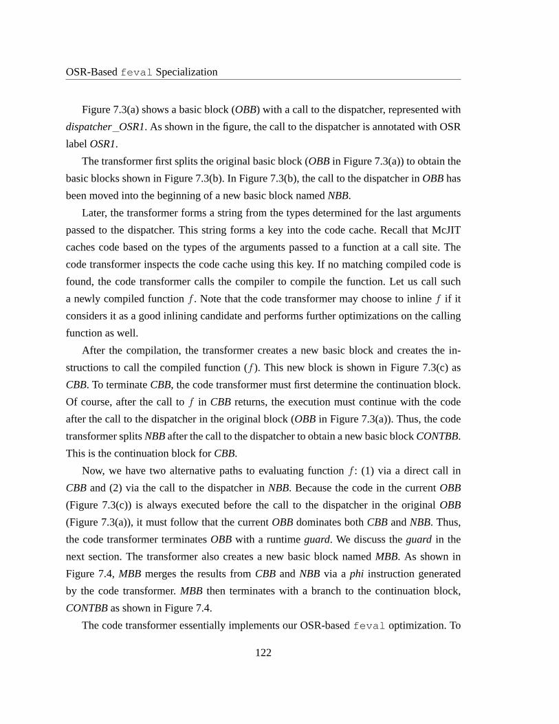
OSR-Basedfeval Specialization
Figure 7.3(a) shows a basic block (OBB) with a call to the dispatcher, represented with
dispatcher OSR1. As shown in the figure, the call to the dispatcher is annotated with OSR
labelOSR1.
The transformer first splits the original basic block (OBB in Figure 7.3(a)) to obtain the
basic blocks shown in Figure 7.3(b). In Figure 7.3(b), the call to the dispatcher inOBBhas
been moved into the beginning of a new basic block namedNBB.
Later, the transformer forms a string from the types determined for the last arguments
passed to the dispatcher. This string forms a key into the code cache. Recall that McJIT
caches code based on the types of the arguments passed to a function at a call site. The
code transformer inspects the code cache using this key. If no matching compiled code is
found, the code transformer calls the compiler to compile the function. Let us call such
a newly compiled functionf . Note that the code transformer may choose to inlinef if it
considers it as a good inlining candidate and performs further optimizations on the calling
function as well.
After the compilation, the transformer creates a new basic block and creates the in-
structions to call the compiled function (f ). This new block is shown in Figure 7.3(c) as
CBB. To terminateCBB, the code transformer must first determine the continuationblock.
Of course, after the call tof in CBB returns, the execution must continue with the code
after the call to the dispatcher in the original block (OBB in Figure 7.3(a)). Thus, the code
transformer splitsNBBafter the call to the dispatcher to obtain a new basic blockCONTBB.
This is the continuation block forCBB.
Now, we have two alternative paths to evaluating functionf : (1) via a direct call in
CBB and (2) via the call to the dispatcher inNBB. Because the code in the currentOBB
(Figure 7.3(c)) is always executed before the call to the dispatcher in the originalOBB
(Figure 7.3(a)), it must follow that the currentOBBdominates bothCBBandNBB. Thus,
the code transformer terminatesOBB with a runtimeguard. We discuss theguard in the
next section. The transformer also creates a new basic blocknamedMBB. As shown in
Figure 7.4,MBB merges the results fromCBB andNBB via a phi instruction generated
by the code transformer.MBB then terminates with a branch to the continuation block,
CONTBBas shown in Figure 7.4.
The code transformer essentially implements our OSR-basedfeval optimization. To
122

7.2. OSR-Basedfeval Transformation
some degree, the runtime performance depends on the cost of evaluating theguard that
determines the execution path taken at run time. We now discuss the functions of theguard.
7.2.5 Runtime Guards
The code transformer generates a runtime guard (shown in Figure 7.3(c)) that will de-
termine the path taken by the program at run time. It chooses from among several guards
depending on the quality of the metadata it retrieved from the call instruction that calls the
dispatcher. In Section 7.2.2, we mentioned that we collect avariety of JIT compilation-time
facts onfeval call sites in the!FI metadata. The second component of the metadata is
an unsigned integer that encodes three bits of information,corresponding to the following
queries.
1. Is the first argument to anfeval call a read-only variable in the function? We shall
denote this query withROQ.
2. Is the first argument a loop constant variable? We shall useLCQ to denote this query.
3. Do all the arguments to thefeval call have a fixed runtime type? We shall denote
this with FTQ.
The first two pieces of information are computed at JIT compilation time using standard
flow analyses. The third is computed using McJIT’s type inference [CBHV10], which starts
with the actual runtime types for all arguments to the function and infers a set possible
types for each variable at every program point. Therefore atthe call to anfeval , the type-
inference can determine the set of possible types for all thearguments to thefeval call.
If only one type exists in the type set for each argument, thenFTQ is true.
The combination of these queries guides the choice of the guards generated by the
transformer. IfROQ is true, we can move the part of the computation of the guard (to
determine whether or not the runtime value of this argument corresponds to the function
that will be called atCBBshown in Figure 7.4) to the function’s entry block.
If LCQ is true, we can compute the guard outside the loop and use the result to de-
termine the path taken by the program afterOBB. If FTQ is true, it means that all the
123

OSR-Basedfeval Specialization
arguments are monomorphic and we can completely eliminate the check that determines
whether the type of any argument changes at run time. We discuss this further below.
Let
f : denote the first argument to anfeval call;
P : denote the set of the remaining argumentsp2, p3, ...,pn to thefeval call;
lastValue(f): denote the cached value off ;
newValue(f): denote the current value off ;
lastType(p): denote the cached type of variablep;
newType(p): denote the current type of variablep.
FEB: be the entry basic block of a function containing anfeval call; and
LEB: be the entry basic block of a loop with anfeval call.
We enumerate in Table 7.1, the different possible guards (based on the three queries)
that the code transformer can generate together with the optimal point to compute a guard.
To simplify the table, we define
f cond = lastValue(f) == newValue(f)
a cond = ∀(p ∈ P ), lastType(p) == newType(p)
and write f cond (FEB) if f cond should be computed at the entry basic block of the
function containing a correspondingfeval call.
Let us examine Table 7.1. In the first case (i.e., table row 1),ROQ, LCQ, andFTQ are
true, in this case, onlyf cond should be computed and can be done atFEB, that is, the
calling function’s entry basic block.FTQ is true. Thus, we know that the runtime type of
each argument at thefeval call site is fixed so, there is no need to includea condin the
guard that is evaluated atOBB.
In Case 2 (i.e., table row 2), the required guard that the code transformer must generate
is: guard = f cond ∧ a cond. This is because the type of each argument tof may
change at run time. Furthermore, if after transforming the code, the value off changes
(i.e., in a subsequent call of the function with thefeval call), the backup path must be
taken. Thef condcomponent of the guard can be evaluated at the function’s entry basic
124

7.2. OSR-Basedfeval Transformation
# ROQ LCQ FTQ Guard Compute Point
1 T T T f cond f cond(FEB)
2 T T F f cond∧ f cond(FEB);
a cond a cond(OBB)
3 T F T * *
4 T F F * *
5 F T T f cond f cond(LEB)
6 F T F f cond∧ f cond(LEB);
a cond a cond(OBB)
7 F F T f cond f cond(OBB);
8 F F F f cond∧ f cond(OBB);
a cond a cond(OBB)
Table 7.1 – Guard truth table (a “*” denotes an impossible result).
block becausef is read-only in the calling function. It must be a parameter of the function.
However, because the types of the arguments may change before thefeval call site, the
second component of the guard,a cond, must be evaluated just before the use of the guard
in basic blockOBB.
Cases 3 and 4 represent impossible cases because it cannot be that f is a read-only
variable in the calling function and at the same time not be a loop constant in that function.
In Case 5, onlyf condshould be computed and this can be done atLEB.
Case 6 is similar to Case 2 except thatROQ is false, meaning thatf is not a read-
only variable but it is a loop constant. For this reason, likeCase 2, the required guard is
guard= f cond∧ a cond. Unlike Case 2, however, the optimal point to computef cond
is atLEB. The second component (a cond) must still be computed atOBB.
In Case 7, we know that the arguments have constant types at thefeval call site. But
we also know thatf is neither a read-only nor a loop constant. So, the required guard is to
evaluate onlyf condatOBBbefore the use of the guard.
Case 8 requires that bothf condanda condbe computed atOBB before the use of
the guard in the block. This is becausef is neither a read-only nor a loop constant variable.
125

OSR-Basedfeval Specialization
Further, the types of the arguments may change at run time as indicated by the value of
FTQ in row 8 of Table 7.1. Observe that this is the most expensive guard computation the
code transformer can generate.
The least expensive guard is in Case 1. This is the ideal case. In the worst case (Case
8), the code transformer inserts a relatively expensive guard at the end ofOBB that tests
whether the current runtime value offef (of an feval call) corresponds to the compiled
function and that the remaining arguments have stable types. This may have an impact on
performance, although we believe this seldom happens within the class of the applications
that we have considered.
7.2.6 Resuming Execution after an OSR is Triggered
You will note that we have only focused on defining the OSR points and the transfor-
mation that occurs when an OSR triggers, but have not defined how the newly transformed
code is executed and how the state is restored or how control flow is correctly resumed.
These important details are handled automatically by the McOSR library [LH13].
7.3 Experimental Results
In Section 6.1, we demonstrated thatfeval resulted in significant overheads, and that
replacing anfeval by a direct call resulted in substantial speedups, which could be further
increased by inlining the direct call. In this section we examine the performance improve-
ments achieved through our OSR-based specialization presented in Section 7.2. We exam-
ine both the benefits and limitations of the approach, and we compare its performance with
the upper bound speedups provided under the hand-coded direct call and inlined versions.
In Table 7.2, the column labelledBaselineshows the results of executing the bench-
marks with McVM JIT in the normal mode. The columns labelledOSR-based Optimiza-
tion give the execution times for three variations of the OSR approach.Opt0 gives the
results when the benchmarks were run with our basic OSR-basedfeval optimization en-
abled. We also experimented with two further improvements.The column labelledOpt1
shows the benchmarks with the OSR-basedfeval optimization plus a dynamic function
126

7.3. Experimental Results
Baseline OSR-based Optimization Hand-coded
t(s) t(s) Speedup Speedup
Benchmark Baseline(F) Opt0 Opt1 Opt2 F/Opt0 F/Opt1 F/Opt2 F/D F/I
bisect 2.38 1.93 1.92 1.93 1.23 1.24 1.23 1.41 2.22
newton 2.60 2.23 2.23 1.55 1.17 1.17 1.68 1.85 3.56
odeEuler 4.61 2.71 2.82 2.64 1.71 1.63 1.75 7.97 6.29
odeMidpt 7.10 4.22 4.18 4.15 1.68 1.70 1.71 10.56 10.91
odeRK4 12.79 7.35 7.46 7.36 1.74 1.72 1.74 18.88 19.22
gaussQuad 1.27 1.03 1.04 1.05 1.23 1.22 1.21 1.31 1.32
sim 3.47 3.40 3.36 2.98 1.02 1.03 1.16 1.38 1.57
Geometric Mean 1.37 1.36 1.47 3.58 4.16
Table 7.2 – Overall results for OSR-based optimitimzation inMcVM JIT
inlining optimization that is performed when the OSR point triggers.Opt2 is a further im-
provement where we first apply the dynamic inlining, and thenapply a further optimization
of the symbol table environment, which is sometimes enabledby the inlining. We describe
this optimization in more detail in our discussion of the performance of this optimization.
From the results, we found that ourfeval optimization was effective. McJIT with the
feval optimization consistently outperforms the standard McVM JIT on our benchmark
set. The geometric mean of speedups atOpt0 is 1.37. The dynamic inlining optimization
enabled byOpt1 does not improve performance on its own, but in combination with the
subsequent symbol table optimization enabled forOpt2, there is an improvement, with a
geometric mean speedup of 1.47.
At optimization level 2 (Opt2), we recorded the highest performance improvements
with the newtonand sim benchmarks. In McVM, the interaction between the compiled
code and the interpreter is often facilitated through a symbol look-up environment. A sym-
bol environment is a table that associates a value to a symbol. It is used to bind a value to
a variable, and to look-up the value of a variable at run time.When needed, McJIT inserts
the instructions to set up a symbol look-up environment for afunction at the function’s pro-
logue. The set-up code initializes the environment for subsequent look-ups and bindings of
values to variables. This can be a major source of overhead. After dynamic inlining, we
127

OSR-Basedfeval Specialization
perform an optimization that eliminates redundant set-up code. We found that the interac-
tion simplification was particularly effective in two of thebenchmarks:newtonandsim,
which contained significant redundant setup code after inlining.
Although speedups of 1.47 are good, it is also important to examine if our dynamic
optimization is approaching the upper bound speedups that we measured by hand-coding
the direct call and hand-lining that call. The last two columns show the speedups we had
measured for the hand-coded versions, and we see that the geometric mean speedups were
3.58 for the direct call and 4.16 for the inlined call. Thus, there is still a significant gap
between what the dynamic technique achieves and the upper bound.
To see why this is the case, we examined the kinds of the runtime guards and the LLVM
code generated for our benchmarks. We show the kinds for eachbenchmark in Table 7.3,
with column# feval (in loop)showing the number offeval calls in the loops of a bench-
mark. We show the kinds of the runtime guards generated for the feval calls in a bench-
mark under columnTypes of Guards.
Benchmark # feval Types of
(in loop) Guards
bisect 1 Case 1a
newton 1 Case 2b
odeEuler 1 Case 2
odeMidpt 2 Case 2
odeRK4 4 Case 2
gaussQuad 1 Case 1
sim anl 1 Case 1
a. According to Table 7.1, Case 1 means that only the value of the fef is checked
at the function’s entry basic block. The types of the arguments to thefeval call are
stable.b. According to Table 7.1, Case 2 means that the value of thefef is checked at the
function’s entry basic block; while the types of all the arguments are checked in the
loop containing thefeval call.
Table 7.3 – Types of the runtime guards used by each benchmark.
128

7.4. Summary
We can see from Table 7.3 that a somewhat expensive guard — onethat checks the
value of thefef passed in at theentrybasic block and the types ofall the arguments to an
feval call in a loop — is generated for eachfeval call in theodebenchmarks. This is the
case because the type inference engine infers that the type of at least one of the arguments
is variable orunknown. This can be a source of runtime overhead. In addition, because the
type-inference infers that the type of an argument to the target function of eachfeval
call in theodebenchmarks is variable, the LLVM code generated for theodebenchmarks
is less efficient. This is the main reason for the relatively lower performance recorded for
the OSR-based version running the actualodebenchmarks. We continue this discussion
in Section 8.2.2, where we compare the performance results discussed here with those
obtained for the benchmarks under our second mechanism forfeval call specialization.
We conclude that converting an indirect call to a direct callcan reveal good optimiza-
tion opportunities that may be exploited for a performance improvement. Our OSR-based
feval optimizing transformation technique is effective and practical. We will continue to
improve our optimizer and we believe that our technique can be used to improve perfor-
mance in similar JIT compilers.
7.4 Summary
We proposed a general on-the-fly mechanism for specializingfeval calls in hot loops
using the OSR mechanism available in McVM, an open source research virtual machine
for MATLAB. We demonstrated good performance improvements using the approach.
In the next chapter, we present a different approach that uses parameter values to spe-
cialize functions withfeval calls. We then compare the performance of this new approach
with our OSR-based approach.
129

OSR-Basedfeval Specialization
130

Chapter 8
JIT Value-Based Specialization
We presented in Chapter 7, the first of our two approaches to specializing feval
calls. In this chapter, we present the second approach, which extends the McJIT type-
specialization mechanism. The approach named JIT value-based approach specializes func-
tions withfeval calls using the runtime values of the arguments to the function. It is based
on the observation that, for some class of MATLAB programs, afunction with anfeval
call often accepts as an argument the name or the function handle to a function evaluated by
the feval call. Further, the call is often executed repeatedly withina long-running loop,
which, as we showed in Chapter 6, can cause a major performanceslow down.
The main contributions of this chapter are:
JIT value-based specialization:We designed an extension to the McVM JIT specializa-
tion mechanism. Previously specialization was performed based only on the dynamic
typesof function arguments. In the new approach, we also specialize on thevalueof
a function argument, for the case where that argument is usedas the first argument to
a call tofeval inside the body of the function to be compiled.
Implementation in McVM/McOSR: We implemented the proposed approaches in
McVM. Our implementation is open source.
Experimental results: We evaluated the JIT value-based approach. We also comparedthe
JIT value-based approach with the OSR-based approach presented in Chapter 7.
131

JIT Value-Based Specialization
Our JIT-time code specialization forfeval replaces calls to a function that has an
feval call with a call to a special dispatch function. This dispatch function (called the
dispatcher for short) evaluates the value of the parameter that corresponds to anfef. It then
generates a new version of the function with all thefeval calls replaced with direct calls
to thefef. This is illustrated in Figure 8.1.
caller(...)
g(myFunc, ...);
(a)
g(func, ...)
r = feval(func, x, ...);
(b)
g′(func, ...)
r = myFunc(x, ...);
(c)
Figure 8.1 –feval Runtime Code Specialization.
In Figure 8.1, functioncaller calls functiong. As shown in (b), functiong has anfeval
call that evaluates one of its parameters, namelyfunc. Functioncaller calls g with an ar-
gument,myFunc, which references a function (e.g., a function handle or a function name).
This is the function that thefeval call in g will evaluate.
However in Figure 8.1(c), a new version of functiong namedg′ is created and all the
feval calls that evaluatefunchave been replaced with direct calls to functionmyFunc.
In the next section, we describe in detail the implementation of this approach.
8.1 JIT Code Specialization
During the parsing of the XML string for a compilation unit (i.e., a list of MATLAB
functions in a MATLAB mfile (Figure 2.3)), McJIT analyzes allthe functions in the com-
pilation unit and annotates those with anfeval call, whosefef, that is, the first parameter,
is a read-only parameter of the enclosing function.
Normally, after McJIT has compiled the right version of a function at a call site, it
inserts the corresponding LLVM call instruction into the current basic block. However, to
132

8.1. JIT Code Specialization
support the runtime code specialization forfeval , we modified McJIT so that it does not
insert the call instruction but, instead, generates a new instruction of the form
call void @''JITExt::dispatchFunction'' (i8* %baseIRPtr,i8* %fefValue,i8* %inArgsPtr ,i8* %retValsPtr ,i32 %csID)
that calls the dispatcher. The dispatcher, that is, function JITExt::dispatchFunction, ac-
cepts five arguments:
(1) the first is the pointer to the base IR (i.e., the original version of the IR) that corresponds
to the called function at the call site;
(2) the second is a pointer to the argument that corresponds to the fef (i.e., the first param-
eter) of a markedfeval call in the called function;
(3) the third is a pointer to a structure containing the input arguments to the called function;
(4) the fourth is a pointer to a structure containing the return values;
(5) the last argument is an integer that denotes the index of a cache slot where a pointer to
the descriptor of the AST can be located.
Each AST representing a function with anfeval call has one or more code cache
descriptors. A code cache descriptor contains informationrelated to the code of the AST
that corresponds to the types of the arguments passed to the function at a call site.
A function that is called with different argument types at different call sites has a code
cache descriptor for each call site. A code cache descriptoris a four-tuple.
descriptor = < entry address, argument types,
counter, feval versions>
whereentry addressis the address of the entry to the compiled code corresponding to the
AST of the called function. We shall denote the called function at a call site withf . Field
argument typesdenotes the types of the arguments at the call site. Due to McJIT’s code
specialization on argument types at call sites, the set of types for the arguments at a call
133

JIT Value-Based Specialization
site is immutable. Fieldcounterdenotes a compilation counter that counts the number of
versions that are generated at different consecutive executions of the call to the dispatcher
instruction. Fieldfeval versionsis a map containing (AST, entry address) pairs. The first
member of the pair is the IR corresponding to the value of the parameter used as the first
argument to somefeval calls inf . The second member of the pair is the address of the
entry point to the compiled code off that corresponds to anfef.
8.1.1 Functions of the Dispatcher
At run time, the dispatcher first uses a combination of its first parameter (i.e., the AST)
and its last parameter (i.e., the cache slot index) to retrieve the code cache descriptor that
matches the argument types at the current call site. This is shown in line 1 of Algorithm 2.
Then, in line 2, the dispatcher performs a look-up using its second parameter to determine
whether a corresponding code version had been generated.
If the look-up is successful, the dispatcher executes (in line 13 of Algorithm 2) the
function at the address returned by the look-up.
Otherwise, the dispatcher compares the current value of thecounter in the code cache
descriptor with a giventhreshold. If the counter has exceeded the threshold, the dispatcher
executes the initial code generated for the AST at this call site. This is shown in line 15
of Algorithm 2. If the counter is below the threshold, however, the dispatcher clones the
original AST and replaces all the markedfeval calls with direct calls to the evaluated
function given as its second parameter. After, the dispatcher retrieves the types attached to
this call site and calls the compiler to compile and generatethe correct code matching the
argument types at this call site. These actions are performed in lines 3 – 11 of Algorithm 2.
After the compilation of a new version, the dispatcher inserts an entry — that is, a pair
comprising of the AST corresponding to the current value of the fef and the entry point
address of the compiled code — into a map in the code cache descriptor of the base IR.
This action is performed by the call of functionputNewVersionin line 9 of Algorithm 2.
The dispatcher does this so that if the function is called again with the samefef value, it can
retrieve and execute the correct code. Finally, the dispatcher updates the counter associated
with the cache slot descriptor.
134

8.1. JIT Code Specialization
input : baseIR, fef, inArgPtr, outArgPtr, cacheSlot
output: void
1 ci← getCodeCacheInfo (baseIR, cacheSlot);
2 entryPoint← lookupFunction (ci, fef);
3 if entryPoint == NULL AND ci.counter<= THRESHOLD then
4 newIR← clone (baseIR);
5 replaceFevalCalls (newIR, fef);
6 llvmIR← compileFunction (newIR, ci.argTypesStr);
7 entryPoint← compCallWrapper (llvmIR, newIR, ci.argTypesStr);
8 // insert an entry for a new version into the cache;
9 putNewVersion (ci, getFunction (fef), entryPoint);
10 ci.counter← ci.counter + 1;
11 end
12 if entryPoint 6= NULL then
13 call entryPoint (inArgsPtr, outArgsPtr);
14 else
15 call ci.entryPoint(inArgsPtr, outArgsPtr);
16 end
Algorithm 2: dispatch function
135

JIT Value-Based Specialization
Although the base AST and new versions of the AST have the samenumber of input and
output parameters, the types of the values returned by the compiled code that corresponds
to a givenfef may be different. This presents a problem in that the rest of the code of
the calling function was generated using the information obtained from the base AST.
We resolved this problem by generating a wrapper (line 7 of Algorithm 2) that converts
from the types returned by a new version to the types used in generating the code for the
original version. Because of this problem, we always call thecode that matches anfef via
a wrapper.1 A wrapper is a short function. It is composed of a call instruction and the
instructions that convert the return values to their expected types.
A code cache look-up miss causes a compilation of a new version if the value of the
counter in the code cache descriptor has not exceeded the threshold. After the counter
has exceeded the given threshold, the dispatcher stops compiling new versions. Thus, for
a newfef value, the dispatcher then always executes the original code generated for the
base AST of the called function. This scheme can prevent excessive compilation actions in
cases where too many different functions are being called. However, this rarely happens in
practice. So, we expect only a reasonable number of new versions to be generated.
Again, we stress that this approach only works in cases wherethefef of anfeval call
in the called function is a read-only function parameter. This covers most of the programs
under study. In Section 8.2.2, we compare the performance ofthis approach with that of
our OSR-based approach that we described in Chapter 7.
8.1.2 General Dispatcher
We can extend Algorithm 2 to cover more cases of JIT value-based specialization. Al-
gorithm 3 shows a more general dispatcher. Here, we have replaced the input parameter
namedfef in Algorithm 2 withV . The general dispatcher specializes the called function us-
ing the runtime values ofV . We have also replaced the calls to functionreplaceFevalCalls
andgetFunctionin Algorithm 2 with calls to functiontransformIR(line 5) andmakeKey
(line 9) in Algorithm 3 respectively.
1. Instead of using a wrapper, our future implementations will use a specialized compiler that directly
performs the type conversion in the generated specialized version.
136

8.1. JIT Code Specialization
input : baseIR, V, inArgPtr, outArgPtr, cacheSlot
output: void
1 ci← getCodeCacheInfo (baseIR, cacheSlot);
2 entryPoint← lookupFunction (ci, V);
3 if entryPoint == NULL AND ci.counter<= THRESHOLD then
4 newIR← clone (baseIR);
5 transformIR (newIR, V);
6 llvmIR← compileFunction (newIR, ci.argTypesStr);
7 entryPoint← compCallWrapper (llvmIR, newIR, ci.argTypesStr);
8 // insert an entry for a new version into the cache;
9 putNewVersion (ci, makeKey (V), entryPoint);
10 ci.counter← ci.counter + 1;
11 end
12 if entryPoint 6= NULL then
13 call entryPoint (inArgsPtr, outArgsPtr);
14 else
15 call ci.entryPoint(inArgsPtr, outArgsPtr);
16 end
Algorithm 3: A more general dispatch function
137

JIT Value-Based Specialization
As an example of an application of the general dispatcher, consider the MATLABeval
(many dynamic languages have a similar feature as well). TheMATLAB eval built-in
evaluates MATLAB code given as its input string expression.Like the feval specializa-
tion, in some cases, we can also specialize a function with aneval call whose input string
is a parameter of the function by developing a suitableIR transformerfor the specialization.
Another example is the specialization of a function with a parameter that is an array.
We can specialize the function using the properties of the array, such as array bounds, to
generate more efficient code for loops that operate on such anarray in the body of the
function.
8.2 Experimental Results
We have described the implementation of our JIT value-basedspecialization approach.
We shall now evaluate its performance over the existing McJIT with no feval call spe-
cialization. Later, we shall compare the performance of theJIT value-based specialization
with the OSR-based specialization approach.
8.2.1 JIT value-based-specialization approach
The OSR-based approach (Section 7.2) is general-purpose, and can operate on any
feval within a loop. However, our results show that there is still agap between the perfor-
mance of the OSR-approach and the upper bound. The value-specialization (Section 8.1)
approach applies to a common case where thefef of the feval call is a read-only pa-
rameter of the enclosing function. In these cases the value-specialization can generate a
completely specialized version of the function, without the need for run-time guards, and
in which the JIT-time type and shape analysis can operate more accurately.
In Table 8.1, we show the results of the value-based specialization in a context where
we can compare it to both the hand-coded, and OSR-based results. The column labelled
VB-specialization gives the time and the speedup relative to the baseline. We note that
this gives excellent results, with speedups approaching the hand-coded upper bound for all
the benchmarks. The value-based results gave a geometric mean speedup of 3.22, which is
138

8.2. Experimental Results
Benchmark Baseline OSR-based (OPT0) VB-Specialization Hand-coded (D)
t(s) t(s) speedup t(s) speedup t(s) speedup
bisect 2.38 1.93 1.23 1.66 1.43 1.68 1.42
newton 2.60 2.23 1.16 1.61 1.61 1.40 1.85
odeEuler 4.61 2.70 1.71 0.67 6.86 0.58 7.97
odeMidpt 7.10 4.22 1.68 0.83 8.53 0.67 10.56
odeRK4 12.79 7.35 1.74 0.89 14.30 0.68 18.88
gaussQuad 1.27 1.03 1.23 0.90 1.41 0.97 1.31
sim 3.47 3.40 1.02 2.60 1.33 2.51 1.38
Geometric Mean 1.37 3.22 3.58
Table 8.1 – Comparing Value-based specialization to OSR-based and hand-coded
substantially better than the 1.37 for the OSR-based approach, and almost as good as the
upper bound of 3.58.
Under the JIT value-based specialization approach, the specialized versions of the func-
tions with feval calls may no longer containfeval calls. Thus, allowing McJIT to
generate much more efficient code. TheodeRK4benchmark has fourfeval calls within
a long-running loop. These calls are replaced with direct calls in the specialized version
generated at run time. Because thefeval target function (fef) is now known, the type in-
ference engine can analyze the function more precisely, andMcJIT can then generate more
efficient code for both the target function and the calling function.
8.2.2 A comparison of the OSR-based and JIT value-based-
specialization approaches
To understand in more detail why the value-based approach provides better perfor-
mance, we need to examine the quality of the LLVM code generated for each benchmark,
and the sources of overheads under the two approaches.
Under the OSR-based approach, McJIT generates less efficientcode. This is so because
McJIT generates a call to the interpreter for anfeval call afterboxingthe arguments to
the feval call to make them more generic. In addition, because the called function (fef)
139

JIT Value-Based Specialization
at the call site is unknown during the compilation time, the type inference engine is unable
to infer precise types for the values returned by thefeval call, thus forcing the compiler
to generate more generic instructions that are suitable forhandling different types. This is
a major source of inefficiency in the OSR-based approach.
Runtime guard computation can be expensive. The OSR-based approach generates run-
time guards, which, as discussed in Section 7.2.5, depend onwhether or not the arguments
to anfeval call have a fixed type. As mentioned in Section 7.3, for the threeodebench-
marks, the type inference engine infers that the types to allthe feval calls are variable,
forcing the code transformer to generate an expensive guardfor eachfeval call special-
ization.
We examinedodeRK4. The code snippet for the only loop of the benchmark is shown
in Listing 8.1.
Listing 8.1 – TheodeRK4benchmark (from [Rec00a,Rec00b]).1 for j=2:n2 k1 = feval ( diffeq , t ( j−1), y( j−1) );3 k2 = feval ( diffeq , t ( j−1)+h2, y(j−1)+h2*k1 );4 k3 = feval ( diffeq , t ( j−1)+h2, y(j−1)+h2*k2 );5 k4 = feval ( diffeq , t ( j−1)+h, y( j−1)+h*k3 );6 y( j ) = y( j−1) + h6*(k1+k4) + h3*(k2+k3);7 end
In the firstfeval call (line 2), the type inference engine infers thatt ( j−1) is a scalar
floating point value. It, however, infers thaty( j−1) can either be a scalar floating point
value or a scalar complex value. In all the remaining threefeval calls (lines 3 – 5), the
type inference engine infers that the second parameter is a floating point value, but infers
unknownfor the third parameter.
Thus, in specializing the fourfeval calls inodeRK4, the code transformer inserts an
expensive guard for each call specialization. The guards generated correspond to Row 2
of Table 7.1, that is,f cond is evaluated at the function’s entry basic block anda cond is
evaluated in the loop.
The JIT value-based approach is less affected by the foregoing issues. If all thefeval
calls in a function have the samefef and thefef is a read-only parameter of the function,
140

8.3. Summary
then the specialized code generated to match thefef at run time will not contain anyfeval
call implementation. Eachfeval call in the AST of the function would have been replaced
with a direct call to thefef. This allows the type inference engine to analyze the calledfunc-
tion, which, in turn, allows McJIT to further specialize thecall site and generate efficient
code. Thefeval calls in all the benchmarks have theirfefs passed in as a parameter, thus
contributing to the generation of the more efficient code forthe specialized versions.
It is, however, true that the JIT value-based approach incurs some runtime overheads,
including that of the code cache look-up. But this is small given the expected gains. Further,
unlike the OSR-based approach that is limited to specialization of feval calls within a
long-running loop, the JIT value-based approach can specialize a function with anfeval
call that occurs anywhere within the body of the function.
We conclude that although the JIT value-based approach is less powerful than the OSR-
based approach, it is more effective on our benchmark set. The JIT approach only works
where thefef is passed as a read-only parameter to a function. It does not work if the fef
is a local variable in the function with thefeval call. The OSR-based approach works
in all cases but incurs much larger runtime overhead. It is possible to combine the two
approaches in a JIT compiler by first analyzing a function with anfeval call to determine
whether a call of the function can benefit from the JIT value-based specialization approach.
With speedups of up to 14 times faster, it would seem that suchtechniques are well worth
incorporating into JIT compilers for MATLAB and other dynamic languages which have
compute-intensive solvers which are abstracted over the computation function (fef).
8.3 Summary
We introduced an effective JIT value-based specializationtechnique for optimizing
feval calls, whose first argument is a function parameter. This is an alternative approach
to the OSR-based on-the-fly mechanism for specializingfeval calls in hot loops dis-
cussed in Chapter 7. We showed how the JIT value-basedfeval specialization can be
extended to handle more cases of JIT value-based specialization in a MATLAB JIT com-
piler. The approach can also be used for JIT value-based specialization in other similar
141

JIT Value-Based Specialization
dynamic languages as well. Indeed, the OSR-based approach can be similarly extended.
We collected a set of seven typical benchmarks that usefeval , and demonstrated that
our specialization approaches provide significant speedups over the basefeval imple-
mentation for this benchmark set. In some cases the performance is near to the optimal
performance of a hand-inlined function, but in other cases agap remains. We would like to
continue to develop new optimizations to further close thatgap, and to apply the same sort
of transformations to other dynamic features in MATLAB.
A somewhat surprising discovery in this work was the complexinterplay between the
JIT-time interprocedural type analysis and the on-the-fly transformations. The JIT value-
based specialization can replacefeval calls with direct calls in a function body, before
doing the type analysis of that function body, thus leading to much better specialized code
(because the interprocedural analysis can handle the direct calls much more precisely). On
the other hand, this specialization can only happen at the function level, and only when the
feval target function corresponds to a read-only parameter. The OSR-based method is
more general, and can be applied at the level of loops, but suffers from less precise type
information. It would be interesting to look at future work that combine the strengths of
both approaches.
142

Chapter 9
Related Work
The work presented thus far in this thesis builds upon the strength of other work in
the literature. Therefore, in this chapter, we present the work upon which this thesis has
been developed. First, we discuss the work that are related to our array copy optimization
approach. Second, we describe the work that are related to our OSR approach and show
how our system is different from the past work on OSR. Third, wediscuss the work related
to our OSR-based dynamic inlining approach. Fourth, we review the past work related to
our feval call specialization approach. We conclude the chapter witha review of the work
related to our JIT value-based code specialization approach for functions withfeval calls.
Before we present the related work, it is important to note that unlike dynamic opti-
mization systems such as Dynamo [BDB00] that work on the nativeinstruction stream, our
transformations and optimizations are performed only at the intermediate-representation
level.
9.1 Copy Optimization
Redundant copy elimination is a hard problem and implementations of languages such
as Python [pyt12] are able to avoid copy elimination optimizations by providing multiple
data structures: some with copy semantics and others with reference semantics. Program-
mers decide when to use mutable data structures. However, efficient implementations of
languages like the MATLAB programming language that use copy semantics require copy
143

Related Work
elimination optimization. The problem is similar to the aggregate update problem in func-
tional languages [HB85, GH89, Ode91, Sas94, WC01]. To modify anaggregate in a strict
functional language, a copy of the aggregate must be made. This is in contrast with the
imperative programming languages where an aggregate may bemodified multiple times.
APL [Ive62] is one of the oldest array-based languages. Weigang [Wei85] describes a
range of optimizations for APL compiler, including a copy optimization that finds uses of
a copy of a variable and replaces the copy with the original variable wherever possible. We
implemented this optimization as part of our QuickCheck phase. We found the optimiza-
tion effective at enabling the elimination of redundant copy statements by the dead-code
optimizer. However, this optimization is unable to eliminate redundant copies of arguments
and return values. Hudak and Bloss [HB85] use an approach basedon abstract interpreta-
tion and conventional flow analysis to detect cases where an aggregate may be modified
in place. Their method combines static analysis and dynamictechniques. It involves a re-
arrangement of the execution order or an optimized version of reference counting, where
the static analysis fails. Our approach is based on flow analysis but we do not change the
execution order of a program.
The interprocedural aliasing and side-effect problem [Muc97] is related to the copy
elimination problem. By using call by reference semantics, when an argument is passed
to a function during a call, the parameter becomes an alias for the argument in the caller
and if the argument contains an array reference, the referenced array becomes a shared
array; any updates via the parameter in the callee updates the same array referenced by
the corresponding argument in the caller. Without performing a separate and expensive
flow analysis, our approach easily detects aliasing and sideeffects in functions. Wand and
Clinger present [WC01] interprocedural flow analyses for aliasing and liveness based on
set constraints. They present two operational semantics: the first one permits destructive
updates of arrays while the other does not. They also define a transformation from a strict
functional language to a language that allows destructive updates. Like Wand and Clinger,
our approach combines liveness analysis with flow analysis.Unlike Wand and Clinger,
however, our analyses are intraprocedural and have been implemented in a JIT compiler
for an imperative language.
144
9.2. On-Stack Replacement
The work of Goyal and Paige [GP98] on copy optimization for SETL [SDSD86] is par-
ticularly interesting. Their approach combines a RC scheme with static analysis. A com-
bination of must-alias and live-variable analyses is used to identify dead variables and the
program points where a statement that redefines a dead variable can be inserted to facil-
itate destructive updates. Like our approach, this technique is capable of eliminating the
redundant copying of a shared location that can occur duringan update of the location;
however, it is different from our approach. In particular, it generates dynamic checks to
detect when to create copies. As mentioned in Section 3.7, our approach rarely generates
dynamic checks.
9.2 On-Stack Replacement
Holzle et al. [HCU92] used an OSR technique to dynamically de-optimize running
optimized code to debug the executing program. OSR techniques have been in used in
several implementations of Java programming language, including Jikes research VM
[FQ03,AAB+05] and HotSpot [PVC01] to support adaptive recompilation ofrunning pro-
grams. A more general-purpose approach to OSR for the Jikes VM was suggested by So-
man and Krintz [SK06] which decouples OSR from the program code. Our approach is
more similar to the original Jikes approach in that we also implement OSR points via ex-
plicit instrumentation and OSR points in the code. However,we have designed our OSR
points and OSR triggering mechanism to fit naturally into theSSA-form LLVM IR and
tool set. Moreover, the LLVM IR is entirely different from Java byte-code and presents
new challenges to OSR implementation at the IR level (Section 4.3). Our approach is also
general-purpose in the sense that the OSR can potentially trigger any optimization or de-
optimization that can be expressed as an LLVM transform.
Recently, Susskraut et al. [SKW+10] developed a tool in LLVM for making a transition
from a slow version of a running function to a fast version. Like Susskraut et al., our system
is based on LLVM. However, there are significant differencesin the approaches. While
their system creates two versions of the same function statically, and transitions from one
version to another at run time, our proposed solution instruments and recompiles code
145
Related Work
dynamically at run time. This is more suitable for an adaptive JIT. Secondly, the approach
used by Susskraut et al. stores the values of local variables in a specially allocated area that
is always accessible when an old stack frame is destroyed anda new stack frame is created
for the executing function. This requires a special memory management facility beyond that
provided by LLVM. In contrast to their approach, our approach does not require a special
allocation because the stack frame is not destroyed until OSR transition is completed. The
recursive call of the executing function essentially extends the old stack frame. We only
have to copy the old addresses and scalar values from the old stack frame onto the new
stack frame. Finally, another notable difference between our approach and that taken by
Susskraut et al. is that their approach requires instrumenting the caller to support OSR in a
called function. This may result in high instrumentation overhead. In our approach, we do
not instrument a caller to support OSR in a callee.
OSR has been implemented in several virtual machines for JavaScript. Like the Jikes
virtual machine, V8 VM [V8V13] and JavaScriptCore [Jav13] allow transitions to a more
optimized version of a running function and de-optimization to the original version. In
our approach, we allow transitions to a more optimized version and de-optimization to the
last version of the less optimized code. In contrast to thesesystems, our OSR technique
supports a transition from optimize code to more optimized code.
9.3 Selective Dynamic Inlining
Inlining is an important compiler optimization. It has beenused successfully in many
production compilers, especially compilers for object-oriented programming languages.
Several techniques for effective inlining were introducedin the several implementations of
SELF [CU91, HU94]. SELF-93 [HU94] uses heuristics to determine the root method for
recompilation by traversing the call stack. It then in-lines the traversed call stack into the
root method. The HotSpot Server VM [PVC01] uses a similar inlining strategy.
Online profile-directed inlining has been explored in many VMs [CLS00, AFG+00,
AHR02,SYN02,ATBC+03,HG03]. The Jikes research VM [AAB+05] considers the effect
of inlining in its cost-benefit model for recompilation by raising the expected benefit of
146
9.4. OSR-Basedfeval Specialization
recompiling a method with a frequently executed call site. Suganuma et al. report that
for inlining decisions for non-tiny methods, heuristics based solely on online profile data
outperforms those based on offline, static data [SYN02]. Hazelwood and Grove [HG03]
suggest using a combination of profiling data with context sensitivity to guide inlining
decisions. They recorded a good reduction in compilation time and code space.
In our approach, like the HotSpot server compiler [PVC01], weuse an iteration counter
to detect long-running loops and consider calls to small functions occurring in those loops
as good inlining candidates. Further, calls to functions with a symbol environment set-
up code are also considered for inlining, provided that the calling function has a symbol
environment associated with it.
Online profile-directed inlining in a MATLAB compiler has not been reported in the
literature. We expect that by using online profiling information to identify hot call sites and
guide inlining decisions, inlining of the most critical call sites will boost performance.
9.4 OSR-Based feval Specialization
Historically, function dispatch in dynamic languages was implemented with a dis-
patch look-up table. This was found to be slow. More efficientapproaches have emerged;
they often employ a variety of caching techniques to speed uptable look up. Smalltalk-
80 [GR85,Kra83] uses a global cache to improve look up performance.
Our OSR-based approach is more related to the inline caching [DS84b] approach
used in another Smalltalk implementation. Interestingly,the Smalltalk implementation was
based on several studies of Smalltalk programs that revealed that 95% of the time, the
type of a Smalltalk message receiver is constant [DS84b,UP87,Ung87]. Our approaches to
feval optimization are also based on the observation thatfeval calls in most MATLAB
loops have unchanging first argument.
The inline caching technique used in the Smalltalk compilerinvolves caching the ad-
dress of a looked-up method at the call site by modifying the compiled target code on-the-
fly — by overwriting the call instruction. This allows the method to be called directly in
147
Related Work
a subsequent execution, avoiding the need for a look up. It also involves generating addi-
tional code (often called prologue) in the method that teststhat the receiver type is correct
before executing the body of the method. However, if the testdoes not succeed, it calls the
look-up code.
Holzle et al. extended the inline caching technique to handlepolymorphic call sites
by including more than one cached look-up result per call site. This technique is known
as polymorphic inline caching (PIC) [HCU91]. The PIC approachcaches all the receiver
types at a call site in astub that is generated on-the-fly and rebinds the call to the stub
routine.
In contrast to these approaches, our implementation is donecompletely at the LLVM-IR
level, and not at target code level. Without on-stack replacement support [HCU92,PVC01,
FQ03, AAB+05, SK06, LH13, Lam12], it is hard to cache previous functionlook-up result
“inline” (i.e., at the call site). We also do not need additional code in the called function. We
insert runtime guards so that execution can continue with the original call to the dispatcher
if the guard fails. Also our backup path obviates the need to cache look-up results in a stub
as in the PIC case used in the implementations of SELF [CU91,HU94].
Although multi-paradigm programming languages such as Python, JavaScript, and
functional languages, including Lisp, Haskell, Scheme support higher-order functions, the
function arguments are directly evaluated at run time and often lead to runtime code gen-
eration that is typically supported by polymorphic type inference, and sometimes, binding
time analysis [NN91]. The MATLABfeval is an overloaded built-in that accepts a func-
tion name as a string or function handle and indirectly evaluates, at run time, the function
argument. Our approaches are supported by a type-inferenceanalysis, although it is explicit
that thefeval built-in evaluates functions only. Our approaches are aimed at improving
JIT compiled code, and facilitating efficient compilation of the MATLAB feval , which
can be extended to handle similar features in other dynamic languages, where it would have
otherwise appeared impossible.
To the best of our knowledge, we are not aware of any work on optimization technique
for feval in a JIT compiler for MATLAB.
148

9.5. JIT Value-Based Specialization
9.5 JIT Value-Based Specialization
In a SELF [Cha92] compiler, Chambers and Ungar [CU89] customizethe method called
at a call site to a specificreceivertype. SELF is a pure object-oriented programming lan-
guage. Like Chambers and Ungar, Chevalier-Boisvert et al. customize a called function at
a call site in the McVM JIT compiler [CBHV10]. They, however, based their customiza-
tion on the set of inferred types forall the arguments to the called function at the call site.
Our JIT value-based specialization approach tofeval call optimization in the McVM JIT
compiler extends this type specialization further with a customization based on the runtime
value of an argument that corresponds to a target function ofan feval call in the called
function.
Systems such astcc [PEK97], Tempo[CHM+98], Dyc [GMP+00] use annotations to
express code on which dynamic compilation should be performed. Muth et al. [MWD00]
use profiling and runtime guards to determine when specialized code should be used. In
our case, we neither use user-level annotations to mark coderegion nor profile the runtime
values of variables that can reference a function that is a target of anfeval call. Rather,
we replace a call to the version of the called function that isalready specialized to a fixed
set of argument types (the initial version) with a call to a generic dispatch function. At run
time, we generate a specialized version of the called function using the value passed in to
the parameter that is a target of anfeval call within the function. We use a small look-
up table to cache or select the correct version to dispatch atrun time. If the value varies
frequently, we stop generating new versions and instead start executing the initial version.
The use of templates to reduce runtime code generation overhead has been thoroughly
investigated [CN96,CHM+98,APC+96,CEA+95]. Templates are sequence of instructions
with holes in place of some values [LL96]. We explored the use of templates to reduce
runtime code generation overhead at the LLVM IR level.
If, instead of using the AST, we can generate an LLVM-code template for a function
with an feval call whose target function is a parameter, we can significantly reduce the
cost of generating the LLVM code for a specialized version atrun time. We can achieve this
by simply copying the template and replacing thehole in the copy with the known value of
the parameter corresponding to the target function of thefeval call.
149

Related Work
For our implementation, however, we found that generating an efficient template ahead
of time is often not possible. This is because the name, and therefore, the precise types of
the return values of a function that is a target of anfeval call are generally unknown at
that time. This causes the compiler to generate generic codethat can handle different types
for the operations that depend on those values after the call. The code generated at run time
from the AST benefits greatly from the type information produced by the type-inference
engine after it has analyzed the now known target of anfeval call and the caller as well.
It is possible, using partial evaluation [JGS93] techniques similar to that used in the
FABIUS compiler [LL96], to generate ahead of time specialized versions of a function
with an feval call whose target function is a parameter, provided that some values of
the feval target function can be determined ahead of time. We do not usethis approach
because it can lead to a large increase in compilation time and the creation of code that is
never executed.
150

Chapter 10
Conclusions and Future Work
We discussed several compilation and performance challenges for a MATLAB JIT com-
piler, and presented a collection of novel techniques that address the challenges. Our tech-
niques use runtime information about program behaviour to support on-the-fly program
transformations and optimizations in a JIT compiler for theMATLAB language. Some of
the techniques are supported by our new JIT-time static flow analyses.
Throughout the thesis, we demonstrated through experiments that measured different
aspects of our approaches. We found that our techniques can be used to obtain good perfor-
mance in a JIT compiler for the MATLAB language and other similar dynamic languages.
We discussed an approach to using JIT-time static analyses to enable an efficient im-
plementation of array copy semantics in a MATLAB JIT compiler. We developed four
JIT-time static analyses to support a staged approach to copy optimization. The first stage
is supported by two fast and effective analyses, and the second stage is supported byNec-
essary CopyandCopy Placementanalyses. We found that this approach generates as many
copies as the reference-counting approach and with no runtime check.
As we have explained, on-the-fly transformations and optimizations often require on-
stack replacement, but implementing on-stack replacementcan be very challenging. We
proposed, designed and developed a modular approach to implementing on-stack replace-
ment that can easily be added to a JIT compiler developed in LLVM, without the need to
re-build the underlying LLVM libraries. This was an important step towards the realization
of the on-the-fly techniques presented in this thesis. We showed, using a case study, how
151

Conclusions and Future Work
our OSR approach can be used to support selective dynamic inlining of hot call sites in
long-running loops. We also presented how to leverage the OSR implementation to support
other on-the-fly optimizations such as thefeval call specialization.
We demonstrated that dynamic function evaluation via MATLAB feval can cause sig-
nificant overheads in interpreters and JIT compilers. We presented two new techniques for
optimizing suchfeval calls. We explained the first mechanism, which uses OSR to spe-
cialize feval calls in long-running loops, and gave evidence to show that this technique
can lead to significant performance gains. We also describedand discussed the second
mechanism, which is less general but more effective than thefirst approach. It specializes
a function with anfeval call whose target function is a parameter of the function. It
uses the argument passed into the parameter for the specialization. We found this particular
technique to be highly effective on our benchmark set.
We compared the OSR-based approach with JIT value-based approach and found that
the latter is much more effective than the former. The JIT value-based approach can trans-
form anfeval call located anywhere within a function provided that the target function of
thefeval call is a read-only parameter of the enclosing function. It benefits much from the
more precise runtime-type information that McJIT uses to generate more efficient code at
run time. The OSR-based approach, however, can transform anfeval call located within
a loop body whether or not the target function is a read-only parameter of the function, but
suffers from less precise type information.
The ideas presented in this thesis have been influenced mainly by many research work
in object-oriented languages — both static and dynamic. We reviewed the literature and
presented the main work related to ours. For MATLAB, we are notaware of any work on
on-the-fly transformations and optimizations for a MATLAB JIT compiler. Thus, our re-
search work is the first in this area, and we hope that our work will inspire other researchers
as well.
We implemented OSR for the LLVM JIT compiler toolkit. Our copy optimization and
feval call specialization techniques have been implemented in McJIT. Our implementa-
tion is available as open source software.
152

10.1. Future Work
10.1 Future Work
Here, we highlight the direction for the future work of the research presented in this
thesis.
Copy Optimization: The copy optimization [LH11] works on shared arrays. If an up-
date is made to a shared array, the whole array is copied. Thisworks well for one-
dimensional arrays. However, if the array is multi-dimensional, the whole array will
still be copied even when the update affects a location in oneof the dimensions only.
It would be nice to extend our copy optimization approach to allow sharing of arrays
based on array dimensions. This will reduce the amount of data copied when a shared
array is updated.
On-stack replacement: Our current approach to on-stack replacement assumes that the
application is single-threaded. This is sufficient for our JIT compiler for the MAT-
LAB programming language and other similar languages. To bemore useful to the
larger programming language and virtual machine communities, however, it would
be nice to extend our approach with the capability of handling multi-threaded appli-
cations.
feval call specialization: We discussed the strengths and limitations of both the OSR-
based and JIT value-based approaches to specializingfeval calls in long-running
loops. We believe that these two approaches can be combined and extended to support
more runtime value-based specializations in JIT compilersfor dynamic languages, in
particular, for the MATLAB language.
As we mentioned in Chapter 7, one interesting area of further optimization is MAT-
LAB eval . MATLAB eval is more general than MATLABfeval ; it can evaluate
MATLAB code in a string expression. An analysis of this string can reveal certain
patterns of usage common to MATLAB programs, which can provide opportunities
for specialization in some cases. Indeed, for a MATLAB JIT compiler, more inter-
esting value-based specializations can be performed usingloop and array properties,
such as loop and array bounds.
153
Conclusions and Future Work
McJIT’s type inference engine [CBHV10] has some limitations.One of which is its
inability to propagate array shape information. By enhancing the type inference engine with
the capability to infer array shape information, more loop-based on-the-fly transformations
and optimizations that use array shape information can be developed.
154

Bibliography
[AAB +05] B. Alpern, S. Augart, S. M. Blackburn, M. Butrico, A. Cocchi, P. Cheng,
J. Dolby, S. Fink, D. Grove, M. Hind, K. S. McKinley, M. Mergen, J. E. B.
Moss, T. Ngo, and V. Sarkar. The Jikes Research Virtual Machine Project:
Building an Open-Source Research Community.IBM Syst. J., 44(2):399–
417, 2005.
[ABB+99] E. Anderson, Z. Bai, C. Bischof, S. Blackford, J. Demmel, J. Dongarra,
J. Du Croz, A. Greenbaum, S. Hammarling, A. McKenney, and D. Sorensen.
LAPACK Users’ Guide. SIAM, Philadelphia, USA, third edition, 1999.
[ADDH10] Toheed Aslam, Jesse Doherty, Anton Dubrau, and Laurie Hendren. Aspect-
Matlab: An Aspect-Oriented Scientific Programming Language. InProceed-
ings of the 9th International Conference on Aspect-OrientedSoftware Devel-
opment, March 2010, pages 181–192.
[AFG+00] Matthew Arnold, Stephen Fink, David Grove, Michael Hind, and Peter F.
Sweeney. Adaptive Optimization in the Jalapeno JVM. In Proceedings of
the 15th ACM SIGPLAN Conference on Object-Oriented Programming, Sys-
tems, Languages, and Applications, Minneapolis, Minnesota, United States,
2000, OOPSLA ’00, pages 47–65. ACM, New York, USA.
[AHR02] Matthew Arnold, Michael Hind, and Barbara G. Ryder. Online Feedback-
Directed Optimization of Java. InProceedings of the 17th ACM SIGPLAN
155
Bibliography
Conference on Object-oriented programming, Systems, Languages, and Ap-
plications, Seattle, Washington, USA, 2002, OOPSLA ’02, pages 111–129.
ACM, New York, USA.
[AP02] George Almasi and David Padua. MaJIC: Compiling MATLAB for Speed and
Responsiveness. InProceedings of the ACM SIGPLAN 2002 Conference on
Programming Language Design and Implementation, Berlin, Germany, 2002,
PLDI ’02, pages 294–303. ACM, New York, USA.
[APC+96] Joel Auslander, Matthai Philipose, Craig Chambers, SusanJ. Eggers, and
Brian N. Bershad. Fast, effective dynamic compilation. InProceedings of the
ACM SIGPLAN 1996 Conference on Programming Language Design and Im-
plementation, Philadelphia, Pennsylvania, USA, 1996, PLDI ’96, pages 149–
159. ACM, New York, NY, USA.
[ATBC+03] A.R. Adl-Tabatabai, J. Bharadwaj, D.Y. Chen, A. Ghuloum, V.Menon,
B. Murphy, M.J. Serrano, and T Shpeisman. StarJIT: A Dynamic Compiler
for Managed Runtime Environments.Intel Technology Journal, 7(1):19–31,
Feb 2003.
[ATCL+98] Ali-Reza Adl-Tabatabai, MichałCierniak, Guei-Yuan Lueh, Vishesh
M. Parikh, and James M. Stichnoth. Fast, effective code generation in a
Just-In-Time Java compiler.ACM SIGPLAN Notices, 33(5):280–290, 1998.
[AWZ88] B. Alpern, M. N. Wegman, and F. K. Zadeck. Detecting equality of variables
in programs. InProceedings of the 15th ACM SIGPLAN-SIGACT Symposium
on Principles of Programming Languages, San Diego, California, USA, 1988,
POPL ’88, pages 1–11. ACM, New York, NY, USA.
[Ayc03] John Aycock. A brief history of just-in-time.ACM Computing Surveys,
35(2):97–113, June 2003.
[BBH+13] Matthias Braun, Sebastian Buchwald, Sebastian Hack, Roland Leißa,
Christoph Mallon, and Andreas Zwinkau. Simple and efficient construction
of static single assignment form. In Ranjit Jhala and Koen Bosschere, editors,
Compiler Construction, volume 7791 ofLecture Notes in Computer Science,
pages 102–122. Springer Berlin Heidelberg, 2013.
156

Bibliography
[BDB00] Vasanth Bala, Evelyn Duesterwald, and Sanjeev Banerjia. Dynamo: A Trans-
parent Dynamic Optimization System.ACM SIGPLAN Notices, 35:1–12,
May 2000.
[BS07] Hans-j. Boehm and Michael Spertus. N2310: Transparent
Programmer-Directed Garbage Collection for C++, June 2007.
http://www.open-std.org/jtc1/sc22/wg21/ docs/papers/2007/n2310.pdf.
[BW11] Amy Brown and Greg Wilson.The Architecture Of Open Source Applications.
lulu.com, June 2011.
[CB09] Maxime Chevalier-Boisvert. McVM: An Optimizing VirtualMachine for the
MATLAB Programming Language. Master’s thesis, McGill University, Au-
gust 2009.
[CBHV10] Maxime Chevalier-Boisvert, Laurie Hendren, and Clark Verbrugge. Optimiz-
ing MATLAB through Just-In-Time Specialization. InInternational Confer-
ence on Compiler Construction, March 2010, pages 46–65.
[CEA+95] Craig Chambers, Susan J. Eggers, Joel Auslander, Matthai Philipose, Markus
Mock, and Przemyslaw Pardyak. Automatic dynamic compilation support for
event dispatching in extensible systems. InIN WORKSHOP ON COMPILER
SUPPORT FOR SYSTEMS SOFTWARE, 1995, pages 118–126.
[CFR+89] R. Cytron, J. Ferrante, B. K. Rosen, M. N. Wegman, and F. K. Zadeck. An ef-
ficient method of computing static single assignment form. In Proceedings of
the 16th ACM SIGPLAN-SIGACT Symposium on Principles of Programming
Languages, Austin, Texas, USA, 1989, POPL ’89, pages 25–35. ACM, New
York, NY, USA.
[CH11] Andrew Casey and Laurie Hendren. MetaLexer: A Modular Lexical Speci-
fication Language. InProceedings of the 10th International Conference on
Aspect-Oriented Software Development, March 2011.
[Cha92] Craig David Chambers.The design and implementation of the self compiler,
an optimizing compiler for object-oriented programming languages. PhD
thesis, Stanford, CA, USA, 1992. UMI Order No. GAX92-21602.
157

Bibliography
[CHM+98] C. Consel, L. Hornof, R. Marlet, G. Muller, S. Thibault, E. N.Volanschi,
J. Lawall, and J. Noye. Tempo: Specializing systems applications and beyond.
ACM Computing Surveys, Symposium on Partial Evaluation, 30, 1998.
[Cle04] Cleve Moler.Numerical Computing with MATLAB. SIAM, 2004.
[CLS00] MichałCierniak, Guei-Yuan Lueh, and James M. Stichnoth. Practicing JUDO:
Java Under Dynamic Optimizations. InProceedings of the ACM SIGPLAN
2000 Conference on Programming Language Design and Implementation,
Vancouver, British Columbia, Canada, 2000, PLDI ’00, pages 13–26. ACM,
New York, USA.
[CN96] Charles Consel and Francois Noel. A general approach for run-time special-
ization and its application to c. InProceedings of the 23rd ACM SIGPLAN-
SIGACT Symposium on Principles of Programming Languages, St. Petersburg
Beach, Florida, USA, 1996, POPL ’96, pages 145–156. ACM, New York, NY,
USA.
[CU89] C. Chambers and D. Ungar. Customization: optimizing compiler technology
for self, a dynamically-typed object-oriented programming language. InPro-
ceedings of the ACM SIGPLAN 1989 Conference on Programming Language
Design and Implementation, Portland, Oregon, USA, 1989, PLDI ’89, pages
146–160. ACM, New York, NY, USA.
[CU91] Craig Chambers and David Ungar. Making Pure Object-Oriented Languages
Practical. InConference Proceedings on Object-Oriented Programming Sys-
tems, Languages, and Applications, Phoenix, Arizona, United States, 1991,
OOPSLA ’91, pages 1–15. ACM, New York, USA.
[DS84a] L. Peter Deutsch and Allan M. Schiffman. Efficient implementation of the
smalltalk-80 system. InProceedings of the 11th ACM SIGACT-SIGPLAN
Symposium on Principles of Programming Languages, Salt Lake City, Utah,
USA, 1984, POPL ’84, pages 297–302. ACM, New York, NY, USA.
[DS84b] L. Peter Deutsch and Allan M. Schiffman. Efficient implementation of the
smalltalk-80 system. InProceedings of the 11th ACM SIGACT-SIGPLAN
158
Bibliography
symposium on Principles of programming languages, Salt Lake City, Utah,
United States, 1984, POPL ’84, pages 297–302. ACM, New York, NY, USA.
[EH07] Torbjorn Ekman and Gorel Hedin. The Jastadd Extensible Java Compiler. In
OOPSLA ’07: Proceedings of the 22nd Annual ACM SIGPLAN Conference on
Object-Oriented Programming Systems and Applications, Montreal, Quebec,
Canada, 2007, pages 1–18. ACM, New York, USA.
[FQ03] Stephen J. Fink and Feng Qian. Design, Implementation and Evaluation of
Adaptive Recompilation with On-stack Replacement. InProceedings of the
International Symposium on Code generation and Optimization: Feedback-
Directed and Runtime Optimization, San Francisco, California, 2003, CGO
’03, pages 241–252. IEEE Computer Society, Washington, DC, USA.
[GH89] K. Gopinath and J. L. Hennessy. Copy Elimination in Functional Lan-
guages. InPOPL ’89: Proceedings of the 16th ACM SIGPLAN-SIGACT
Symposium on Principles of Programming Languages, Austin, Texas, United
States, 1989, pages 303–314. ACM, New York, USA.
[GMP+00] Brian Grant, Markus Mock, Matthai Philipose, Craig Chambers, and Susan J.
Eggers. Dyc: an expressive annotation-directed dynamic compiler for c.The-
oretical Computer Science, 248(1-2):147–199, October 2000.
[gnu12] gnu.org. GNU Octave, 2012. http://www.gnu.org/software/octave/index.html.
[Gol73] R. P. Goldberg. Architecture of virtual machines. InProceedings of the Work-
shop on Virtual Computer Systems, Cambridge, Massachusetts, United States,
1973, pages 74–112. ACM, New York, NY, USA.
[GP98] Deepak Goyal and Robert Paige. A New Solution to the Hidden Copy Prob-
lem. In Proc. 5th International Static Analysis Symposium, number1503 in
LNCS, 1998, pages 327–348. Springer-Verlag.
[GR83] Adele Goldberg and David Robson.Smalltalk-80: the language and its im-
plementation. Addison-Wesley Longman Publishing Co., Inc., Boston, MA,
USA, 1983.
[GR85] Adele Goldberg and Divid Robson.Smalltalk-80: The Language and its Im-
plementation. Addison-Wesley, 2 edition, 1985.
159

Bibliography
[HB85] Paul Hudak and Adrienne Bloss. The Aggregate Update Problem in Func-
tional Programming Systems. InPOPL ’85: Proceedings of the 12th ACM
SIGACT-SIGPLAN Symposium on Principles of Programming Languages,
New Orleans, Louisiana, United States, 1985, pages 300–314. ACM, New
York, USA.
[HCU91] Urs Holzle, Craig Chambers, and David Ungar. Optimizing dynamically-
typed object-oriented languages with polymorphic inline caches. InProceed-
ings of the European Conference on Object-Oriented Programming, 1991,
ECOOP ’91, pages 21–38. Springer-Verlag, London, UK, UK.
[HCU92] Urs Holzle, Craig Chambers, and David Ungar. Debugging Optimized Code
with Dynamic Deoptimization. InProceedings of the ACM SIGPLAN 1992
Conference on Programming Language Design and Implementation, San
Francisco, California, United States, 1992, PLDI ’92, pages32–43. ACM,
New York, NY, USA.
[HG03] Kim Hazelwood and David Grove. Adaptive Online Context-Sensitive In-
lining. In Proceedings of the International Symposium on Code Generation
and Optimization: Feedback-Directed and Runtime Optimization, San Fran-
cisco, California, 2003, CGO ’03, pages 253–264. IEEE ComputerSociety,
Washington, DC, USA.
[HU94] Urs Holzle and David Ungar. A Third-Generation SELF Implementation:
Reconciling Responsiveness with Performance. InProceedings of the ninth
Annual Conference on Object-oriented Programming Systems,Language, and
Applications, Portland, Oregon, United States, 1994, OOPSLA ’94, pages
229–243. ACM, New York, NY, USA.
[Int13] ECMA International. Standard ECMA-335,
Common Language Infrastructure (CLI), 2013.
http://www.ecma-international.org/publications/standards/Ecma-335.htm.
[Ive62] Iverson, Kenneth E.A Programming Language. John Wiley and Sons, Inc.,
1962.
160

Bibliography
[Jav13] JavaScriptCore. JavaScriptCore, 2013.
http://trac.webkit.org/wiki/JavaScriptCore/.
[JGS93] Neil D. Jones, Carsten K. Gomard, and Peter Sestoft.Partial evaluation and
automatic program generation. Prentice-Hall, Inc., Upper Saddle River, NJ,
USA, 1993.
[Kay93] Alan C. Kay. The early history of smalltalk. InThe Second ACM SIG-
PLAN Conference on History of Programming Languages, Cambridge, Mas-
sachusetts, USA, 1993, HOPL-II, pages 69–95. ACM, New York, NY, USA.
[KH13] Vineet Kumar and Laurie Hendren. First steps to compiling matlab to x10.
Technical Report sable-2013-01, Sable Researh Group, McGillUniversity,
March 2013.
[Kra83] Glenn Krasner.Smalltalk-80: Bits of History, Words of Advice. Addison-
Wesley, 1983.
[Kra98] A. Krall. Efficient JavaVM Just-in-Time Compilation. In Proceedings of
the 1998 International Conference on Parallel Architectures and Compilation
Techniques, 1998, PACT ’98, pages 205–. IEEE Computer Society, Washing-
ton, DC, USA.
[LA04] Chris Lattner and Vikram Adve. LLVM: A Compilation Framework for Life-
long Program Analysis & Transformation. InCGO ’04: Proceedings of the
International Symposium on Code Generation and Optimization, Palo Alto,
California, 2004, pages 75–86. IEEE Computer Society, Washington, DC,
USA.
[Lam12] Nurudeen Lameed. McOSR: A tool for support-
ing On-Stack Replacement (OSR) in LLVM, 2012.
http://www.sable.mcgill.ca/mclab/mcosr/ .
[LH10] Nurudeen Lameed and Laurie Hendren. Staged Static Techniques to Effi-
ciently Implement Array Copy Semantics in a MATLAB JIT Compiler. Tech-
nical Report SABLE-TR-2010-5, School of Computer Science, McGill Uni-
versity, Montreal, Canada, July 2010.
161
Bibliography
[LH11] Nurudeen Lameed and Laurie Hendren. Staged Static Techniques to Effi-
ciently Implement Array Copy Semantics in a MATLAB JIT Compiler. In
J. Knoop, editor,International Conference on Compiler Construction (CC
2011, LNCS 6601), March 2011, pages 22–41. Springer-Verlag Berlin Hei-
delberg.
[LH13] Nurudeen Lameed and Laurie Hendren. A Modular Approach to On-Stack
Replacement in LLVM. InProceedings of the 9th ACM SIGPLAN/SIGOPS
International Conference on Virtual Execution Enviornments, 2013, VEE ’13,
pages 143–154.
[Li09] Jun Li. McFor: A MATLAB to FORTRAN 95 Compiler. Master’sthesis,
McGill University, August 2009.
[LL96] Peter Lee and Mark Leone. Optimizing ml with run-timecode generation.
SIGPLAN Notices, 31(5):137–148, May 1996.
[llv12] llvm.org. LLVM, 2012. http://www.llvm.org/ .
[LY99] Tim Lindholm and Frank Yellin. Java Virtual Machine Specification.
Addison-Wesley Longman Publishing Co., Inc., Boston, MA, USA, 2nd edi-
tion, 1999.
[Mat09a] MATLAB®7 Getting Started Guide. The MathWorks Inc., 2009.
[Mat09b] MathWorks.MATLAB Programming Fundamentals. The MathWorks, Inc.,
2009.
[mat13] File Exchange, 2013. http://www.mathworks.com/matlabcentral/fileexchange/.
[mc213] Mc2For, 2013.http://www.sable.mcgill.ca/mclab/mc2for.html .
[McC60] John McCarthy. Recursive functions of symbolic expressions and their com-
putation by machine, part i.Communications of the ACM, 3(4):184–195,
April 1960.
[mcl] McLab. http://www.sable.mcgill.ca/mclab/ .
[McL12] McLAB. The McVM virtual machine and its JIT compiler,2012.
http://www.sable.mcgill.ca/mclab/mcvm_mcjit.html .
162

Bibliography
[Mol06] Cleve Moler. The Growth of MATLAB™and
The MathWorks over Two Decades, 2006.
http://www.mathworks.com/company/newsletters/newsnotes/clevescorner/jan06.pdf.
[Moo65] Gordon E. Moore. Cramming more components onto integrated circuits.
Electronics, 38(8), 1965.
[Muc97] S. Muchnick.Advanced Compiler Design and Implementation. Morgan Kauf-
mann, 1997.
[MWD00] Robert Muth, Scott A. Watterson, and Saumya K. Debray.Code specialization
based on value profiles. InProceedings of the 7th International Symposium
on Static Analysis, 2000, SAS ’00, pages 340–359. Springer-Verlag, London,
UK, UK.
[NAJ+75] K. V. Nori, U. Ammann, K. Jensen, H. H. Nageli, and C. Jacobi. The Pascal
P-Compiler: Implementation Notes (rev. ed.). Technical Report 10, Institut
fur Informatik ETH, Zurich, 1975.
[NN91] Hanne Riis Nielson and Flemming Nielson. Using transformations in the im-
plementation of higher-order functions.Journal of Functional Programming,
1:459–494, 1991.
[Ode91] Martin Odersky. How to Make Destructive Updates Less Destructive. In
POPL ’91: Proceedings of the 18th ACM SIGPLAN-SIGACT Symposium
on Principles of Programming Languages, Orlando, Florida, United States,
1991, pages 25–36. ACM, New York, USA.
[PEK97] Massimiliano Poletto, Dawson R. Engler, and M. FransKaashoek. tcc: a
system for fast, flexible, and high-level dynamic code generation. SIGPLAN
Notices, 32(5):109–121, May 1997.
[PG74] Gerald J. Popek and Robert P. Goldberg. Formal requirements for virtualiz-
able third generation architectures.Communications of the ACM, 17(7):412–
421, 1974.
[Pre86] Press, H. William and Teukolsky, A. Saul and Vetterling, T. William and Flan-
nery, P. Brian.Numerical Recipes : the Art of Scientific Computing. Cam-
bridge University Press, 1986.
163

Bibliography
[PVC01] Michael Paleczny, Christopher Vick, and Cliff Click. The Java HotSpot Server
Compiler. InProceedings of the 2001 Symposium on JavaTM Virtual Machine
Research and Technology Symposium - Volume 1, Monterey, California, 2001,
JVM’01, pages 1–12. USENIX Association, Berkeley, CA, USA.
[pyt12] python.org. Python Programming Language, 2012.
http://www.python.org .
[Rec00a] Gerald Recktenwald.Numerical Methods with MATLAB: Implementations
and Applications. Prentice Hall, 2000.
[Rec00b] Gerald Rectenwald. Numerical methods with MATLAB: Im-
plementations and applications (source code distribution), 2000.
http://web.cecs.pdx.edu/ ˜ gerry/nmm/mfiles .
[RGG+96] Luiz De Rose, Kyle Gallivan, Efstratios Gallopoulos, BretA. Marsolf, and
David A. Padua. FALCON: A MATLAB Interactive Restructuring Com-
piler. In LCPC ’95: Proceedings of the 8th International Workshop on
Languages and Compilers for Parallel Computing, 1996, pages 269–288.
Springer-Verlag, London, UK.
[RWZ88] B. K. Rosen, M. N. Wegman, and F. K. Zadeck. Global value numbers and
redundant computations. InProceedings of the 15th ACM SIGPLAN-SIGACT
Symposium on Principles of Programming Languages, San Diego, California,
USA, 1988, POPL ’88, pages 12–27. ACM, New York, NY, USA.
[Sas94] A. V. S. Sastry.Efficient Array Update Analysis of Strict Functional Lan-
guages. PhD thesis, University of Oregon, Eugene, USA, 1994.
[SDSD86] J. T. Schwartz, R. B. Dewar, E. Schonberg, and E. Dubinsky. Programming
with Sets; an Introduction to SETL. Springer-Verlag, New York, USA, 1986.
[SK06] Sunil Soman and Chandra Krintz. Efficient and general on-stack replacement
for aggressive program specialization. InSoftware Engineering Research and
Practice, 2006, pages 925–932.
164
Bibliography
[SKW+10] Martin Susskraut, Thomas Knauth, Stefan Weigert, Ute Schiffel, Martin
Meinhold, and Christof Fetzer. Prospect: A Compiler Framework for Spec-
ulative Parallelization. InProceedings of the 8th Annual IEEE/ACM Inter-
national Symposium on Code generation and Optimization, Toronto, Ontario,
Canada, 2010, pages 131–140. ACM, New York, USA.
[SN05] Jim Smith and Ravi Nair.Virtual Machines: Versatile Platform for Systems
and Processes. Morgan Kaufmann Publishers, 2005.
[SOK+04] T. Suganuma, T. Ogasawara, K. Kawachiya, M. Takeuchi, K.Ishizaki,
T. Koseki, A. an d Inagaki, T. Yasue, M. Kawahito, T. Onodera,H. Komatsu,
and T. Nakatani. Evolution of a Java Just-In-Time compiler for ia-32 plat-
forms. IBM Journal of Research and Development, 48(5/6):767–795, 2004.
[SYN02] Toshio Suganuma, Toshiaki Yasue, and Toshio Nakatani. An Empirical Study
of Method In-lining for a Java Just-In-Time Compiler. InProceedings of the
2nd Java Virtual Machine Research and Technology Symposium, 2002, pages
91–104. USENIX Association, Berkeley, CA, USA.
[Tar74] Robert Tarjan. Finding dominators in directed graphs. SIAM Journal on
Computing, 3(1):62–89, 1974.
[The02] The Mathworks. Technology Backgrounder:
Accelerating MATLAB, September 2002.
http://www.mathworks.com/company/newsletters/digest/sept02/accelmatlab.pdf.
[Ung87] David Michael Ungar. The design and evaluation of a high performance
Smalltalk system. MIT Press, Cambridge, MA, USA, 1987.
[UP87] David Ungar and David Patterson. What price smalltalk? Computer,
20(1):67–74, January 1987.
[V8V13] V8 Virtual Machine, 2013.https://developers.google.com/v8/ .
[WC01] Mitchell Wand and William D. Clinger. Set Constraints forDestructive Array
Update Optimization.Journal of Functional Programming, 11(3):319–346,
2001.
165

Bibliography
[Wei85] Weigang, Jim. An Introduction to STSC’s APL Compiler.SIGAPL APL
Quote Quad, 15(4):231–238, 1985.
[WPD01] R. Clint Whaley, Antoine Petitet, and Jack J. Dongarra. Automated Empirical
Optimizations of Software and the ATLAS Project.Parallel Computing, 27(1-
2):3 – 35, 2001.
[YMP+99] Byung-Sun Yang, Soo-Mook Moon, Seongbae Park, Junpyo Lee, SeungIl
Lee, Jinpyo Park, Yoo C. Chung, Suhyun Kim, Kemal Ebcioglu, andErik
Altman. LaTTe: A Java VM Just-in-Time Compiler with Fast and Efficient
Register Allocation. InProceedings of the 1999 International Conference on
Parallel Architectures and Compilation Techniques, 1999, PACT ’99, pages
128–. IEEE Computer Society, Washington, DC, USA.
166

Appendix A
Relevant McVM compilation flags
Here we present McVM flags related to the work presented in this thesis.
./mcvm -jit_enable true -jit_osr_enable true
-jit_osr_strategy outer
-jit enable: Enables JIT compilation in McVM. The default execution engine is the in-
terpreter. If the flag is set totrue, JIT compilation is used, otherwise, all code will be
interpreted.
-jit osr enable: Enables OSR if JIT compilation is enabled. It is set tofalseby default.
-jit osr strategy: If OSR is enabled, it uses the strategy specified. Another valid option
is inner, which is used to specify that McJIT should insert OSR point in the inner-
most loop of a loop nest. If the specified strategy isouter, McJIT will insert OSR
points in the appropriate outer-most loops.
-jit osr inline: To force dynamic inlining, if OSR is enabled.
167

Relevant McVM compilation flags
168

Appendix B
Copy optimization aspect
In this section, we list theaspectused in estimating the number of copies a MATLAB
program would perform under the reference-counting approach for implementing array
copy semantics in MATLAB system.
169

Copy optimization aspect
1
2 aspect refcounter3
4 % This aspect counts the number of copies generated5 % in a matlab program, using the matlab copy semantics :6 % 'copy on write '.7 % Only copies generated in program functions are8 % considered. Built−in functions may generate further9 % copies. However, such copies are not counted since
10 % aspectMatlab compiler (amc) can not profile11 % built−in functions .12 %13 % Limitations : For accurate result only one user−defined14 % function may be used as a rhs of an15 % assignment statement . Complicated expressions16 % involving multiple user−defined functions17 % should be split into ' simple forms '.18 % However, this does not affect built−ins and19 % matlab−defined m−files.20 %21 % Date: February 2010.22 % Author: Nurudeen Lameed23 % Email: [email protected]
25 properties26 verbose = 0; % # display progress27 matlab builtin home = '/packages/matlab' ; % for builtin28 defs count = 0; % # of definitions29 writes count = 0; % # of array writes30 num copies = 0; % # of copies generated31 m ID gen = 0; % # unique memory id generator32 top = 0; % top of stack pointer33 mem = struct (); % mem ory34 stack = {}; % array of stack frames35
36 % for the current callee37 last assign line = −1;38 multi assign on = 0;39 arg names = {}; % temp for arg names40 param write off = 0; % flag for setting params41 end42
43 methods44 function push( this , s)45 this . top = this . top + 1;46 this .stack { this . top } = s;47 end48
49 function s = pop( this )50 s = this .stack { this . top };
170

51 this . top = this . top − 1;52 end53
54 function retVal = isDefFromFunc(this,line )55 retVal = 0;56 if ( isfield ( this .stack { this . top }, 'last_call_addr_' ))57 lastCallAddr = getfield ( this .stack{ this . top }, ...58 'last_call_addr_' );59 if ( lastCallAddr ==line )60 retVal = 1;61 end62 end63 end64
65 function incrDefsCount( this )66 this .defs count = this .defs count + 1;67 end68
69 function genMem (this, name)70 %generate a new memory space for this name71
72 this .m ID gen = this.m ID gen + 1;73 mID = ['m' , num2str(this.m ID gen )];74 this .mem = setfield( this .mem, mID, 1);75
76 % update the current stackframe77 this .stack { this . top } = setfield ( this .stack{ this . top }, name, mID);78 end79
80 function incrRefCount( this , mID)81 rc = getfield ( this .mem, mID);82 this .mem = setfield( this .mem, mID, rc + 1);83 end84
85 function decrRefCount( this , mID)86 rc = getfield ( this .mem, mID);87 if (( rc − 1) == 0) % garbage ?88 this .mem = rmfield(this .mem , mID);89 else90 this .mem = setfield( this .mem, mID, rc− 1);91 end92 end93
94 function incrCpCount( this , loc , name,line )95 % increment the number of copies96
97 % find the mem ory referenced by this symbol98 mID = getfield ( this .stack{ this . top }, name);99
100 %disp(['memory = ', mID, ' symbol = ', name]);101 %disp( this .mem);
171

Copy optimization aspect
102 %disp( this .stack{ this . top });103 % get the reference count for the object referenced104 rc = getfield ( this .mem, mID);105
106 if ( rc > 1) %perform copy107 if ( this .verbose )108 disp([ 'ARRAY COPY:: (name, line) : (' , name,',' , ...109 num2str(line ), ')' ]);110 end111 this .num copies = this.num copies + 1;112 this .genMem (name);113
114 % update ref count115 this .mem = setfield( this .mem, mID, rc− 1);116 end117 this . incrWritesCount ();118 end119
120 function incrWritesCount( this )121 this .writes count = this .writes count + 1;122 end123
124 function init ( this )125 this .verbose = 1;126 this .matlab builtin home = '/packages/matlab'127 this .defs count = 0;128 this .writes count = 0;129 this .num copies = 0;130 this .m ID gen = 0;131 this . top = 0;132 this .mem = struct ();133 this .stack = {};134
135 % for the current callee136 this . last assign line = −1;137 this .multi assign on = 0;138 this .arg names = {};139 this .param write off = 0;140 end141
142 function printStatistics ( this , name)143 disp([ 'Result for ' , name]);144 disp( '=========================================' );145 disp([ 'Array-definition count: ' , num2str(this.defs count )]);146 disp([ 'Array-write count: ' , num2str(this.writes count )]);147 disp([ 'Total number of copies generated: ' , num2str(this.num copies )]);148
149 % if ( this .verbose )150 % disp (' Mem ory dump');151 % disp( this .mem);152 % end
172
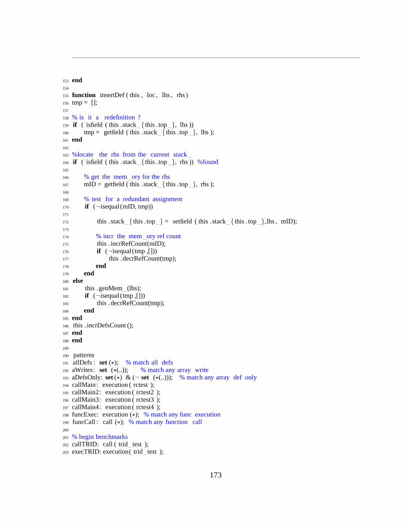
153 end154
155 function insertDef ( this , loc , lhs , rhs )156 tmp = [];157
158 % is it a redefinition ?159 if ( isfield ( this .stack { this . top }, lhs ))160 tmp = getfield ( this .stack{ this . top }, lhs );161 end162
163 %locate the rhs from the current stack164 if ( isfield ( this .stack { this . top }, rhs )) %found165
166 % get the memory for the rhs167 mID = getfield ( this .stack{ this . top }, rhs );168
169 % test for a redundant assignment170 if (¬isequal (mID, tmp))171
172 this .stack { this . top } = setfield ( this .stack{ this . top },lhs , mID);173
174 % incr the mem ory ref count175 this . incrRefCount(mID);176 if (¬isequal (tmp ,[]))177 this .decrRefCount(tmp);178 end179 end180 else181 this .genMem (lhs);182 if (¬isequal (tmp ,[]))183 this .decrRefCount(tmp);184 end185 end186 this . incrDefsCount ();187 end188 end189
190 patterns191 allDefs : set (* ); % match all defs192 aWrites: set (* (..)); % match any array write193 aDefsOnly:set(* ) & (¬ set (* (..))); % match any array def only194 callMain: execution ( rctest );195 callMain2: execution ( rctest2 );196 callMain3: execution ( rctest3 );197 callMain4: execution ( rctest4 );198 funcExec: execution (* ); % match any func execution199 funcCall : call (* ); % match any function call200
201 % begin benchmarks202 callTRID: call ( trid test );203 execTRID: execution( tridtest );
173

Copy optimization aspect
204
205 callADPT: call ( adpt test );206 execADPT: execution(adpttest );207
208 callCAPR: call ( capr test );209 execCAPR: execution(caprtest );210
211 callCLOS: call ( clos test );212 execCLOS: execution(clostest );213
214 callCRNI: call ( crni test );215 execCRNI: execution( crnitest );216
217 callDICH: call ( dich test );218 execDICH: execution(dichtest );219
220 callDIFF: call ( diff test );221 execDIFF: execution ( diff test );222
223 callFDTD: call ( fdtd test );224 execFDTD: execution(fdtdtest );225
226 callFFT: call ( fft test );227 execFFT: execution ( ffttest );228
229 callFIFF : call ( fiff test );230 execFIFF: execution ( fiff test );231
232 callMBRT: call (mbrt test );233 execMBRT: execution(mbrttest);234
235 callNB1D: call (nb1d test );236 execNB1D: execution(nb1dtest);237
238 callNB3D: call (nb3d test );239 execNB3D: execution(nb3dtest);240
241 callNFRC: call ( nfrc test );242 execNFRC: execution(nfrctest );243 % end benchmarks244 end245
246 actions247
248 afterAllDefs : after allDefs :( loc , name, aobj ,line )249 if ( this . last assign line == line && ¬this.param write off )250
251 % multiple assignment detected252 if ( this .verbose )253 disp([ 'multiple assignment in line ' , num2str(line), ...254 ' lhs: ' , name,' position: ' , ...
174

255 num2str(this .multi assign on + 2)]);256 end257
258 if ( this .multi assign on )259 this .multi assign on = this .multi assign on + 1;260 else261 this .multi assign on = 1;262 end263 else264 this . last assign line = line ;265 this .multi assign on = 0;266 end267 end268
269 afterDefsAct : after aDefsOnly: ( loc , name, aobj ,line )270 if ( this .verbose )271 disp([ 'DEF:: (name, line) : (' , name,',' , num2str(line), ')' , ...272 ' = ' , aobj]);273 end274 if ( this .param write off )275 this .param write off = this.param write off − 1;276 elseif ( this . isDefFromFunc(line))277 retCount = getfield ( this .stack{ this . top }, ...278 'ret_cnt_' );279 retValIndex = this .multi assign on + 1;280 if ( retValIndex ≤ retCount)281 if ( isfield ( this .stack { this . top }, name))282 tmp = getfield ( this .stack{ this . top }, name);283 this .decrRefCount(tmp);284 end285 retvar = ['ret_val_' , num2str(retValIndex)];286 %disp([' ret val = ', retvar ]);287 mID = getfield ( this .stack{ this . top }, retvar );288 this .stack { this . top } = setfield ( this .stack{ this . top }, ...289 name, mID);290 end291 else292 this . insertDef ( loc , name, aobj );293 end294 end295
296 afterAWriteAct : after aWrites: ( loc , name,line )297 if ( this .verbose )298 disp([ 'ARRAY WRITE:: (name, line) : (' , name,',' , ...299 num2str(line ), ')' ]);300 end301 if isfield ( this .stack { this . top }, name)% undefined?302 this . incrCpCount(loc , name,line );303 else304 this .genMem (name); % define ...305 end
175

Copy optimization aspect
306 end307
308
309 beforeFuncCallAct: before funcCall : (name, args ,line , ainput )310 val = line ;311 if ( exist(name,'builtin' ) | strfind(which(name), ...312 this .matlab builtin home ))313 val = −1;314 end315
316 this .stack { this . top } = setfield ( this .stack{ this . top }, ...317 'last_call_addr_' , val);318
319 % set the call arg names320 this .arg names = ainput;321 end322
323 afterFuncCallAct : after funcCall : (name, args ,line ) ...324 % do some stack clean up task325 end326
327 beforeFuncExecAct: before funcExec: (name, ainput , args ,line )328 % disp( this .mem);329 if numel(ainput) 6= numel( this .arg names )330 disp([name,':: error: # of args (' , ...331 num2str(numel(ainput)), ...332 ' != # of parameters (' , num2str(numel(this.arg names ))]);333 exit ;334 end335
336 if ( this .verbose )337 disp([ 'pushing a new stack_ frame for ' , name]);338 end339 % create a stack frame for the function340 this .push( struct ());341
342 %process args−> params transition343 for i=1:numel( this .arg names )344 if (isempty( this .arg names {i}))345
346 % generate a new memory for the parameter347 this .genMem (ainput{i});348 else349 %disp(['Arg name ', this .argnames {i}])350 mID = getfield ( this .stack{ this . top − 1}, this .arg names {i});351 this .stack { this . top } = ...352 setfield ( this .stack{ this . top }, ainput{i }, mID);353 this . incrRefCount(mID);354 end355 end356
176

357 % parameter writing off358 this .param write off = numel(this.arg names );359
360 end361
362 afterFuncExecAct: after funcExec: ( loc , name, aoutput , ...363 line )364 if ( this .verbose )365 disp([ 'popping the stack_ frame for ' , name]);366 end367 sframe = this .pop();368 if ( this . top > 0)369
370 % add a return values count to the callers stackframe371 this .stack { this . top } = ...372 setfield ( this .stack{ this . top }, 'ret_cnt_' , ...373 numel(aoutput ));374 for j=1:numel(aoutput)375 mID = getfield (sframe, aoutput{j });376 retvar = ['ret_val_' , num2str(j)];377
378 % copy ret val to the caller ' s stack379 this .stack { this . top } = ...380 setfield ( this .stack{ this . top }, retvar , mID);381 this . incrRefCount(mID);382 end383 end384
385 if ( isfield (sframe, 'last_call_addr_' ))386 sframe = rmfield (sframe,'last_call_addr_' );387 end388
389 if ( isfield (sframe, 'ret_cnt_' ))390 sframe = rmfield (sframe,'ret_cnt_' );391 end392
393 fields = fieldnames (sframe);394 for i=1:numel( fields )395 if ( strfind ( fields{i }, 'ret_val_' ) > 0)396 continue ; %skip it397 end398
399 % get the memory ID400 mID = getfield (sframe, fields{i });401 this .decrRefCount(mID);402 end403
404 if ( this .verbose )405 disp([ 'final stack_ frame for ' , name,':' ]);406 disp(sframe);407 disp([ 'caller''s stack_ frame for ' , name,':' ]);
177
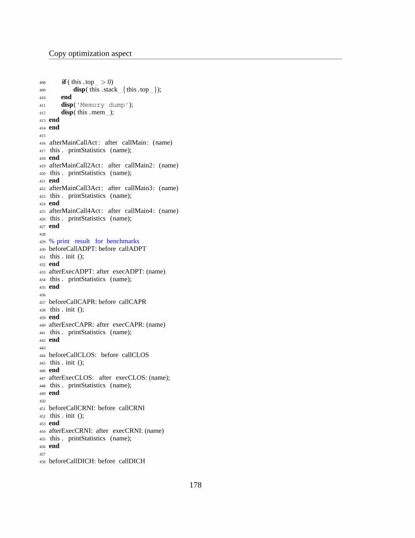
Copy optimization aspect
408 if ( this . top > 0)409 disp( this .stack { this . top });410 end411 disp( 'Memory dump' );412 disp( this .mem );413 end414 end415
416 afterMainCallAct : after callMain: (name)417 this . printStatistics (name);418 end419 afterMainCall2Act : after callMain2: (name)420 this . printStatistics (name);421 end422 afterMainCall3Act : after callMain3: (name)423 this . printStatistics (name);424 end425 afterMainCall4Act : after callMain4: (name)426 this . printStatistics (name);427 end428
429 % print result for benchmarks430 beforeCallADPT: before callADPT431 this . init ();432 end433 afterExecADPT: after execADPT: (name)434 this . printStatistics (name);435 end436
437 beforeCallCAPR: before callCAPR438 this . init ();439 end440 afterExecCAPR: after execCAPR: (name)441 this . printStatistics (name);442 end443
444 beforeCallCLOS: before callCLOS445 this . init ();446 end447 afterExecCLOS: after execCLOS: (name);448 this . printStatistics (name);449 end450
451 beforeCallCRNI: before callCRNI452 this . init ();453 end454 afterExecCRNI: after execCRNI: (name)455 this . printStatistics (name);456 end457
458 beforeCallDICH: before callDICH
178

459 this . init ();460 end461 afterExecDICH: after execDICH: (name)462 this . printStatistics (name)463 end464
465 beforeCallDIFF: before callDIFF466 this . init ();467 end468 afterExecDIFF: after execDIFF: (name)469 this . printStatistics (name);470 end471
472 beforeCallFDTD: before callFDTD473 this . init ();474 end475 afterExecFDTD: after execFDTD: (name)476 this . printStatistics (name);477 end478
479 beforeCallFFT: before callFFT480 this . init ();481 end482 afterExecFFT: after execFFT: (name)483 this . printStatistics (name);484 end485
486 beforeCallFIFF : before callFIFF487 this . init ();488 end489 afterExecFIFF: after execFIFF: (name)490 this . printStatistics (name)491 end492
493 beforeCallMBRT: before callMBRT494 this . init ();495 end496 afterExecMBRT: after execMBRT: (name)497 this . printStatistics (name);498 end499
500 beforeCallNB1D: before callNB1D501 this . init ();502 end503 afterExecNB1D: after execNB1D: (name)504 this . printStatistics (name);505 end506
507 beforeCallNB3D: before callNB3D508 this . init ();509 end
179
Copy optimization aspect
510 afterExecNB3D: after execNB3D: (name)511 this . printStatistics (name);512 end513
514 beforeCallNFRC: before callNFRC515 this . init ();516 end517 afterExecNFRC: after execNFRC: (name)518 this . printStatistics (name);519 end520
521 beforeCallTRID: before callTRID : (name)522 this . init ();523 end524
525 afterExecTRID: after execTRID: (name)526 this . printStatistics (name);527 end528 % end benchmark529 end530 end
180


