1
Disks
Thomas Plagemann with slides from: Pål Halvorsen (Ifi, UiO), Kai Li
(Princeton), Tore Larsen (Ifi/UiTromsø), Maarten van Steen (VU Amsterdam)
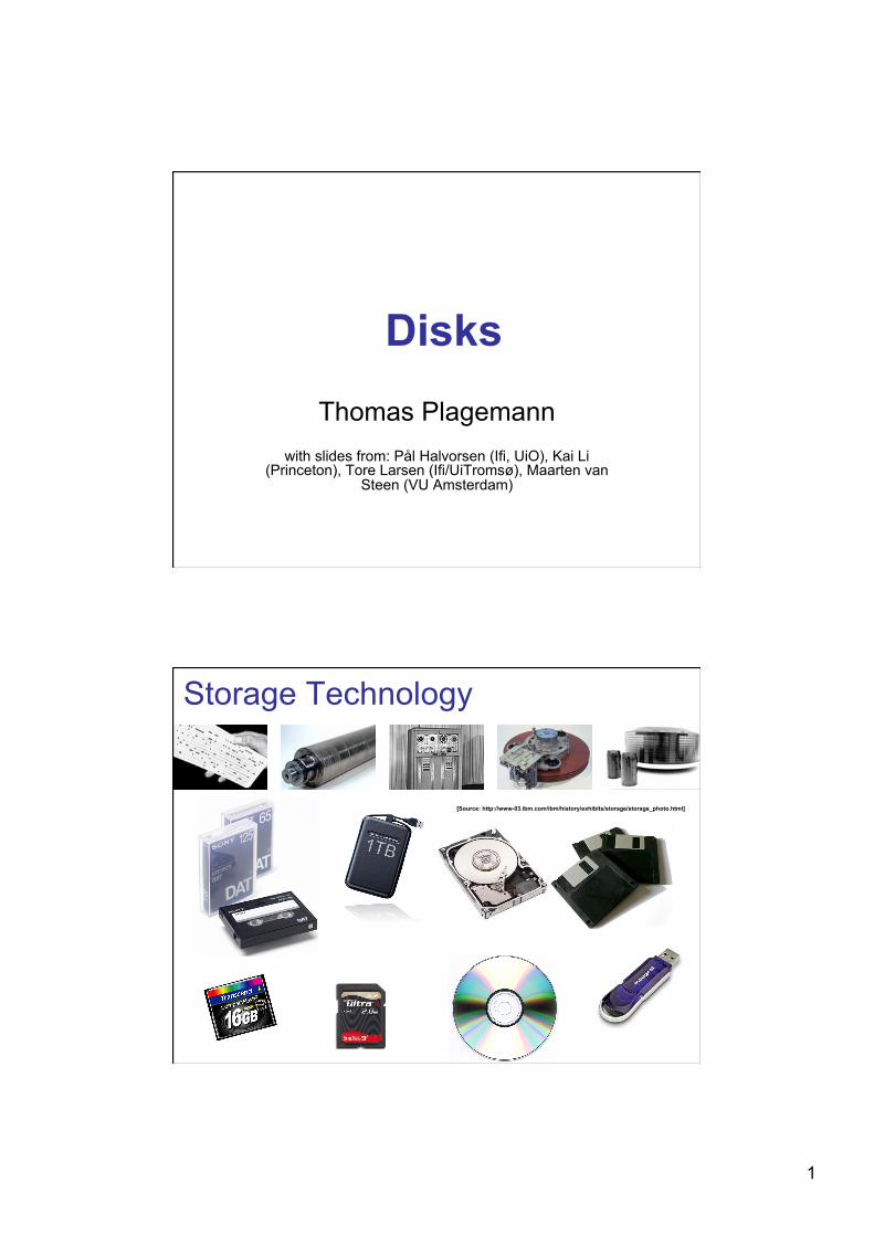
Storage Technology
[Source: http://www-03.ibm.com/ibm/history/exhibits/storage/storage_photo.html]
2
Filesystems & Disks
Contents • Non-volatile storage • Solid State Disks • Disks
- Mechanics, properties, and performance
• Disk scheduling • Additional Material:
Data placement Prefetching and buffering Memory caching Disk errors Multiple disks (RAID)
3
Storage Properties • Volatile and non-volatile
• ROM
• Access (sequential, RAM)
• Mechanical issues
• “Wear out”
Storage Hierarchy • L1 cache • L2 cache • RAM • ROM • EPROM & flash memory (SSD) • Hard disks
• (CD & DVD)
• … and what about Floppy disks?
4
Storage Metrics • Maximum/sustained read bandwidth • Maximum/sustained write bandwidth • Read latency • Write latency
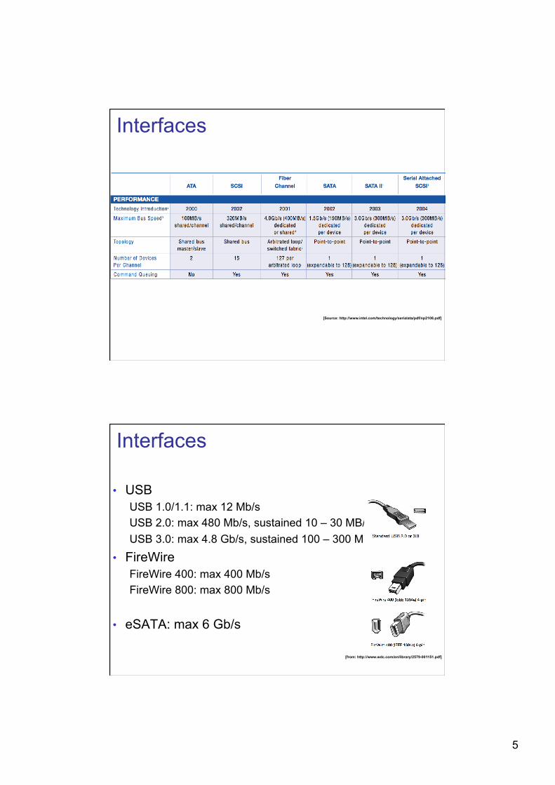
Interfaces • Parallel ATA or simply ATA
• Parallel Small Computer Interface (SCSI)
• Fiber Channel (FC)
• Serial ATA 1.0 (SATA)
• Serial ATA II (SATA II)
• Serial Attached SCSI (SAS)
5
Interfaces
[Source: http://www.intel.com/technology/serialata/pdf/np2108.pdf]
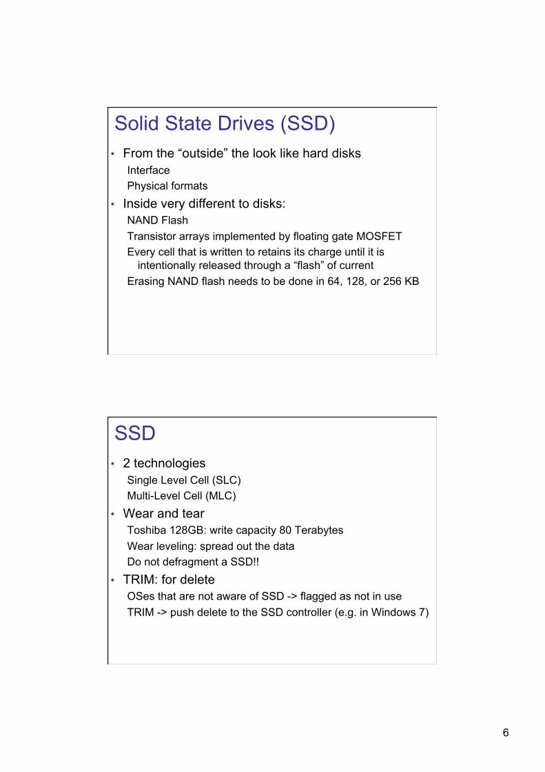
Interfaces
• USB USB 1.0/1.1: max 12 Mb/s USB 2.0: max 480 Mb/s, sustained 10 – 30 MB/s USB 3.0: max 4.8 Gb/s, sustained 100 – 300 MB/s
• FireWire FireWire 400: max 400 Mb/s FireWire 800: max 800 Mb/s
• eSATA: max 6 Gb/s
[from: http://www.wdc.com/en/library/2579-001151.pdf]
6
Solid State Drives (SSD) • From the “outside” the look like hard disks
Interface Physical formats
• Inside very different to disks: NAND Flash Transistor arrays implemented by floating gate MOSFET Every cell that is written to retains its charge until it is
intentionally released through a “flash” of current Erasing NAND flash needs to be done in 64, 128, or 256 KB
SSD • 2 technologies
Single Level Cell (SLC) Multi-Level Cell (MLC)
• Wear and tear Toshiba 128GB: write capacity 80 Terabytes Wear leveling: spread out the data Do not defragment a SSD!!
• TRIM: for delete OSes that are not aware of SSD -> flagged as not in use TRIM -> push delete to the SSD controller (e.g. in Windows 7)
7
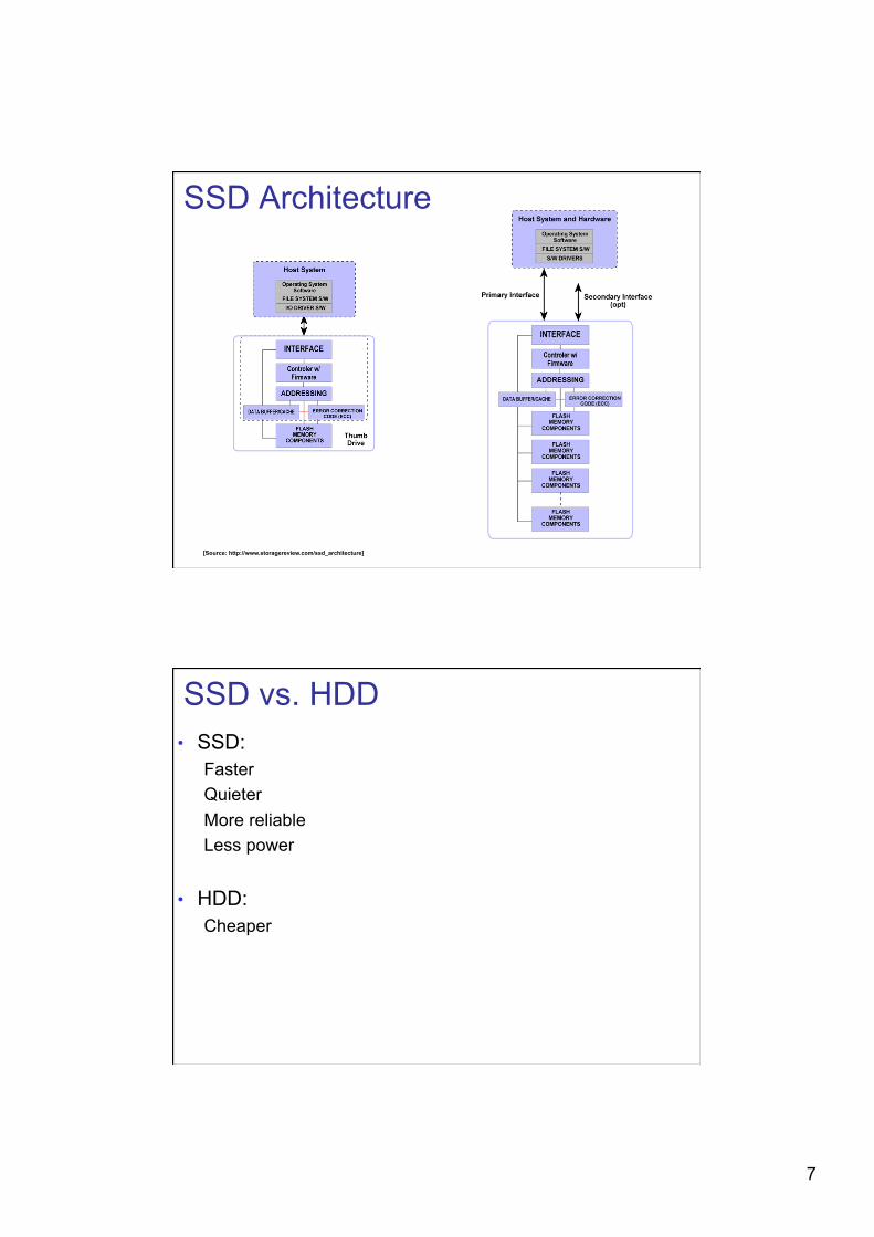
SSD Architecture
[Source: http://www.storagereview.com/ssd_architecture]
SSD vs. HDD • SSD:
Faster Quieter More reliable Less power
• HDD: Cheaper
8
SSD Performance
[Source: http://ssd.toshiba.com/benchmark-scores.html]
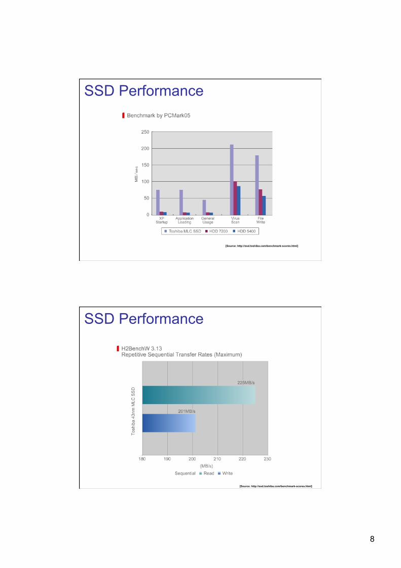
SSD Performance
[Source: http://ssd.toshiba.com/benchmark-scores.html]
9
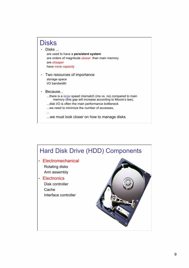
Disks • Disks ...
are used to have a persistent system are orders of magnitude slower than main memory are cheaper have more capacity
• Two resources of importance storage space I/O bandwidth
• Because... ...there is a large speed mismatch (ms vs. ns) compared to main
memory (this gap will increase according to Moore’s law), ...disk I/O is often the main performance bottleneck ...we need to minimize the number of accesses, ... ...we must look closer on how to manage disks
Hard Disk Drive (HDD) Components • Electromechanical
Rotating disks Arm assembly
• Electronics Disk controller Cache Interface controller
10
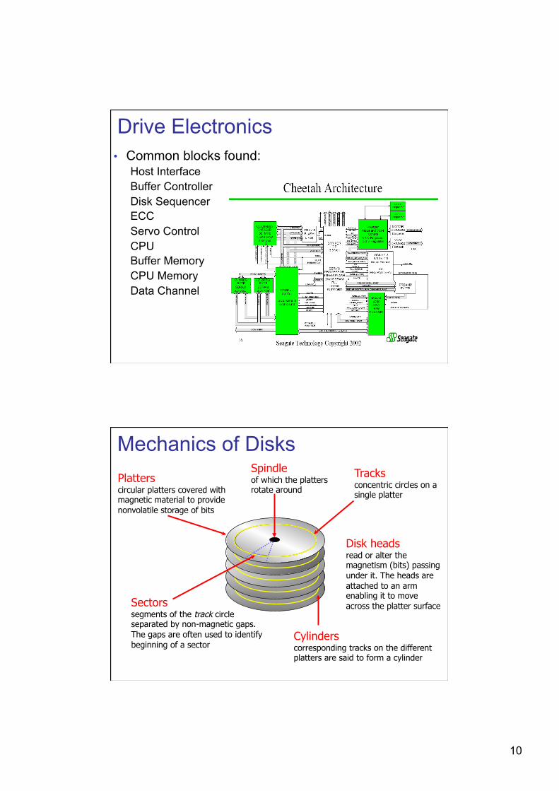
Drive Electronics • Common blocks found:
Host Interface Buffer Controller Disk Sequencer ECC Servo Control CPU Buffer Memory CPU Memory Data Channel
Mechanics of Disks Platters circular platters covered with magnetic material to provide nonvolatile storage of bits
Tracks concentric circles on a single platter
Sectors segments of the track circle separated by non-magnetic gaps. The gaps are often used to identify beginning of a sector
Cylinders corresponding tracks on the different platters are said to form a cylinder
Spindle of which the platters rotate around
Disk heads read or alter the magnetism (bits) passing under it. The heads are attached to an arm enabling it to move across the platter surface
11
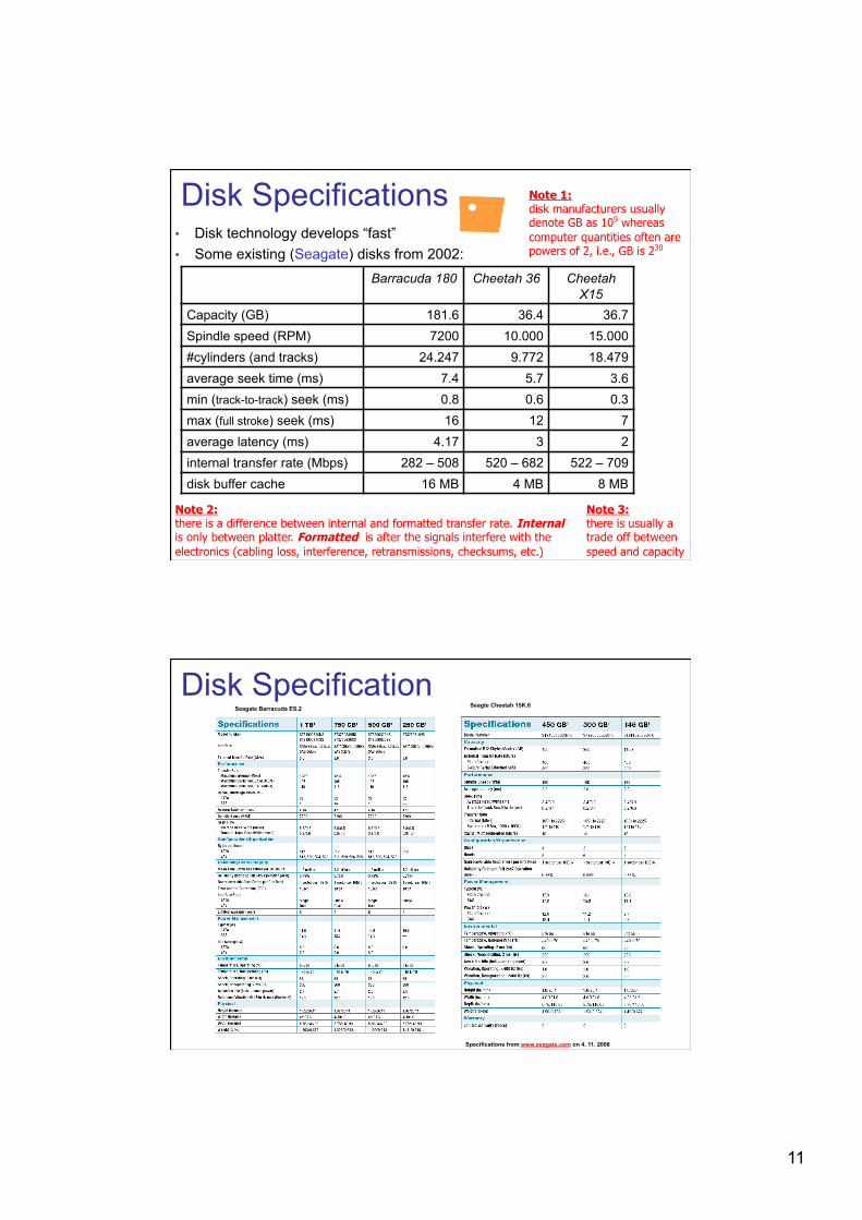
Disk Specifications • Disk technology develops “fast” • Some existing (Seagate) disks from 2002:
Note 1: disk manufacturers usually denote GB as 109 whereas computer quantities often are powers of 2, i.e., GB is 230
Note 3: there is usually a trade off between speed and capacity
Note 2: there is a difference between internal and formatted transfer rate. Internal is only between platter. Formatted is after the signals interfere with the electronics (cabling loss, interference, retransmissions, checksums, etc.)
Barracuda 180 Cheetah 36 Cheetah X15
Capacity (GB) 181.6 36.4 36.7 Spindle speed (RPM) 7200 10.000 15.000 #cylinders (and tracks) 24.247 9.772 18.479 average seek time (ms) 7.4 5.7 3.6 min (track-to-track) seek (ms) 0.8 0.6 0.3 max (full stroke) seek (ms) 16 12 7 average latency (ms) 4.17 3 2 internal transfer rate (Mbps) 282 – 508 520 – 682 522 – 709 disk buffer cache 16 MB 4 MB 8 MB
Disk Specification Seagate Barracuda ES.2 Seagte Cheetah 15K.6
Specifications from www.seagate.com on 4. 11. 2008
12
Disk Capacity • The size (storage space) of the disk is dependent on
the number of platters whether the platters use one or both sides number of tracks per surface (average) number of sectors per track number of bytes per sector
• Example (Cheetah X15): 4 platters using both sides: 8 surfaces 18497 tracks per surface 617 sectors per track (average) 512 bytes per sector Total capacity = 8 x 18497 x 617 x 512 ≈ 4.6 x 1010 = 42.8 GB Formatted capacity = 36.7 GB
Note: there is a difference between formatted and total capacity. Some of the capacity is used for storing checksums, spare tracks, gaps, etc.
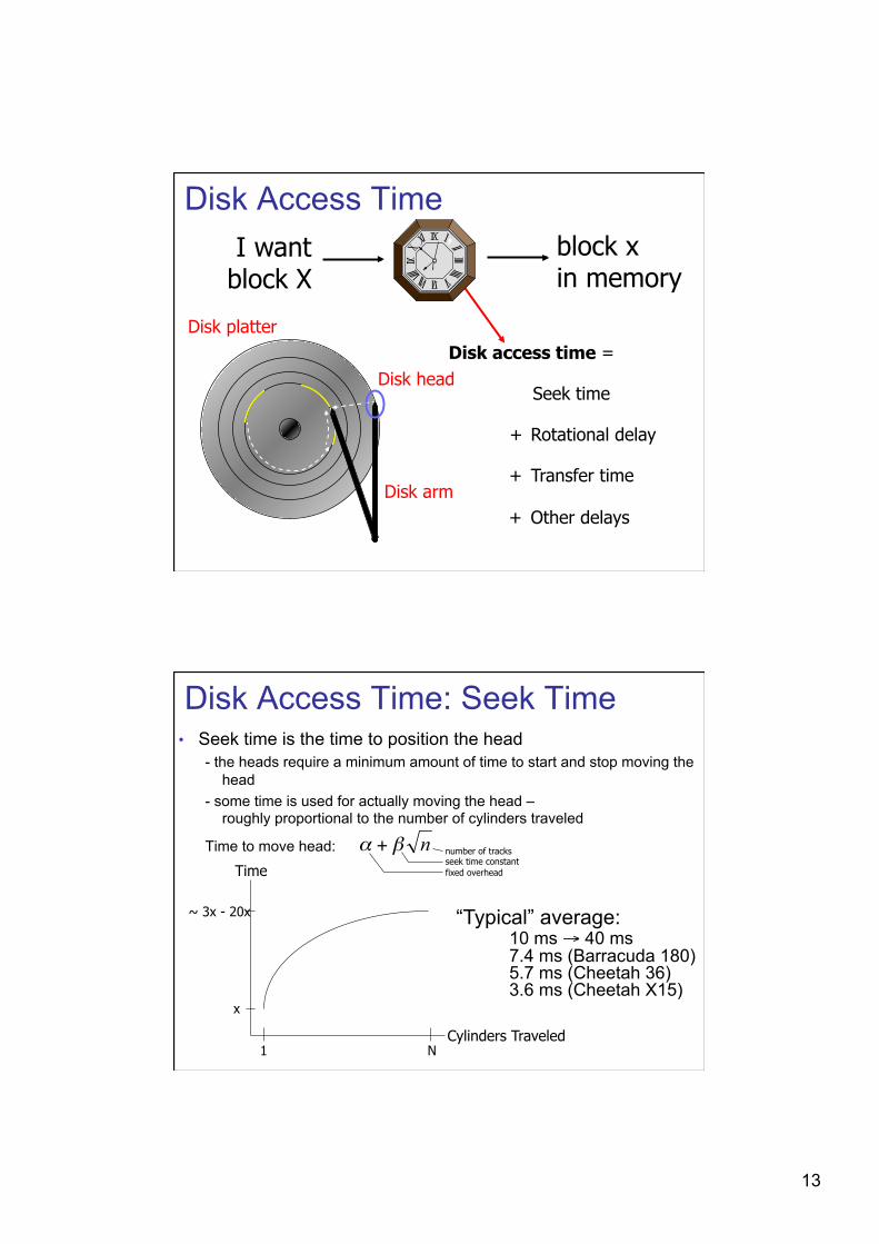
Disk Access Time
• How do we retrieve data from disk? - position head over the cylinder (track) on which the block
(consisting of one or more sectors) are located - read or write the data block as the sectors move under the
head when the platters rotate
• The time between the moment issuing a disk request and the time the block is resident in memory is called disk latency or disk access time
13
+ Rotational delay
+ Transfer time
Seek time
Disk access time =
+ Other delays
Disk platter
Disk arm
Disk head
block x in memory
I want block X
Disk Access Time
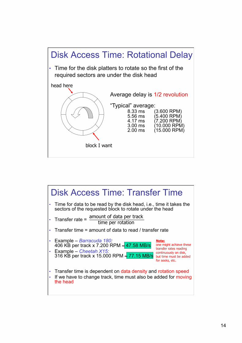
Disk Access Time: Seek Time • Seek time is the time to position the head
- the heads require a minimum amount of time to start and stop moving the head
- some time is used for actually moving the head – roughly proportional to the number of cylinders traveled
Time to move head:
~ 3x - 20x
x
1 N Cylinders Traveled
Time
“Typical” average: 10 ms → 40 ms 7.4 ms (Barracuda 180) 5.7 ms (Cheetah 36) 3.6 ms (Cheetah X15)
number of tracks seek time constant fixed overhead
14
Disk Access Time: Rotational Delay • Time for the disk platters to rotate so the first of the
required sectors are under the disk head
head here
block I want
Average delay is 1/2 revolution
“Typical” average: 8.33 ms (3.600 RPM) 5.56 ms (5.400 RPM)
4.17 ms (7.200 RPM) 3.00 ms (10.000 RPM) 2.00 ms (15.000 RPM)
Disk Access Time: Transfer Time • Time for data to be read by the disk head, i.e., time it takes the
sectors of the requested block to rotate under the head
• Transfer rate =
• Transfer time = amount of data to read / transfer rate
• Example – Barracuda 180: 406 KB per track x 7.200 RPM ≈ 47.58 MB/s
• Example – Cheetah X15: 316 KB per track x 15.000 RPM ≈ 77.15 MB/s
• Transfer time is dependent on data density and rotation speed • If we have to change track, time must also be added for moving
the head
amount of data per track time per rotation
Note: one might achieve these transfer rates reading continuously on disk, but time must be added for seeks, etc.
15
Disk Access Time: Other Delays • There are several other factors which might introduce
additional delays: CPU time to issue and process I/O contention for controller contention for bus contention for memory verifying block correctness with checksums (retransmissions) waiting in scheduling queue ...
• Typical values: “0” (maybe except from waiting in the queue)
Disk Throughput • How much data can we retrieve per second?
• Throughput =
• Example: for each operation we have - average seek - average rotational delay - transfer time - no gaps, etc.
Cheetah X15 (max 77.15 MB/s) 4 KB blocks 0.71 MB/s 64 KB blocks 11.42 MB/s
Barracuda 180 (max 47.58 MB/s) 4 KB blocks 0.35 MB/s 64 KB blocks 5.53 MB/s
data size transfer time (including all)
16
Block Size • The block size may have large effects on performance • Example:
assume random block placement on disk and sequential file access doubling block size will halve the number of disk accesses
each access take some more time to transfer the data, but the total transfer time is the same (i.e., more data per request)
halve the seek times halve rotational delays are omitted
e.g., when increasing block size from 2 KB to 4 KB (no gaps,...) for Cheetah X15 typically an average of:
3.6 ms is saved for seek time 2 ms is saved in rotational delays 0.026 ms is added per transfer time
increasing from 2 KB to 64 KB saves ~96,4 % when reading 64 KB
} saving a total of 5.6 ms when reading 4 KB (49,8 %)
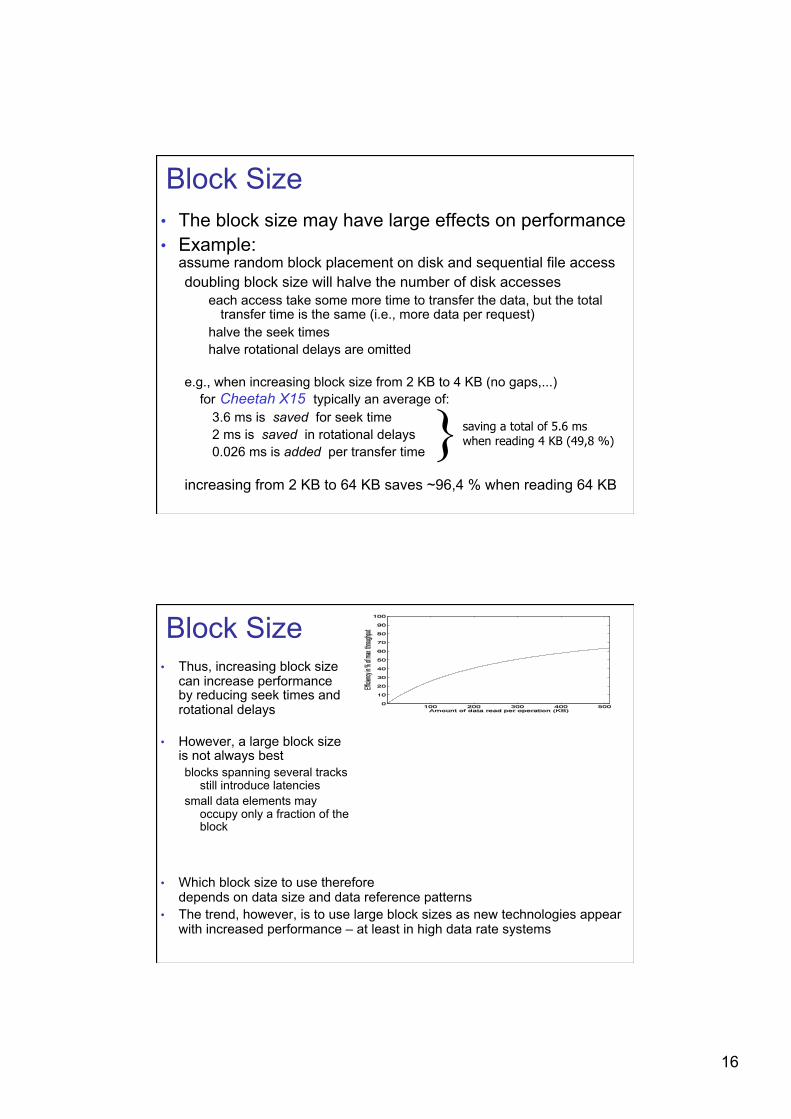
1002003004005000102030405060708090100Amount of data read per operation (KB)Efficiency in % of max. throughput
Block Size • Thus, increasing block size
can increase performance by reducing seek times and rotational delays
• However, a large block size is not always best blocks spanning several tracks
still introduce latencies small data elements may
occupy only a fraction of the block
• Which block size to use therefore depends on data size and data reference patterns
• The trend, however, is to use large block sizes as new technologies appear with increased performance – at least in high data rate systems
17
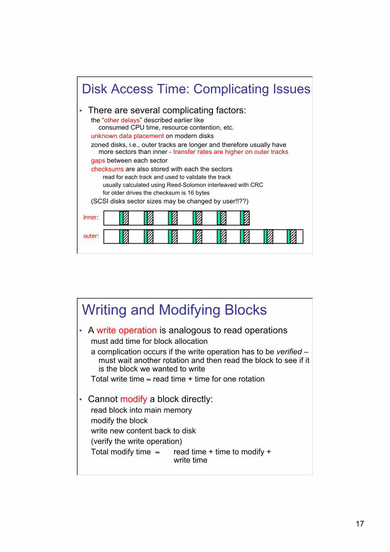
Disk Access Time: Complicating Issues • There are several complicating factors:
the “other delays” described earlier like consumed CPU time, resource contention, etc.
unknown data placement on modern disks zoned disks, i.e., outer tracks are longer and therefore usually have
more sectors than inner - transfer rates are higher on outer tracks gaps between each sector checksums are also stored with each the sectors
read for each track and used to validate the track usually calculated using Reed-Solomon interleaved with CRC for older drives the checksum is 16 bytes
(SCSI disks sector sizes may be changed by user!!??)
inner:
outer:
Writing and Modifying Blocks • A write operation is analogous to read operations
must add time for block allocation a complication occurs if the write operation has to be verified –
must wait another rotation and then read the block to see if it is the block we wanted to write
Total write time ≈ read time + time for one rotation
• Cannot modify a block directly: read block into main memory modify the block write new content back to disk (verify the write operation) Total modify time ≈ read time + time to modify +
write time
18
Disk Controllers • To manage the different parts of the disk, we use a
disk controller, which is a small processor capable of: controlling the actuator moving the head to the desired track selecting which platter and surface to use knowing when right sector is under the head transferring data between main memory and disk
• New controllers acts like small computers themselves both disk and controller now has an own buffer reducing disk
access time data on damaged disk blocks/sectors are just moved to spare
room at the disk – the system above (OS) does not know this, i.e., a block may lie elsewhere than the OS thinks
Efficient Secondary Storage Usage • Must take into account the use of secondary storage
there are large access time gaps, i.e., a disk access will probably dominate the total execution time
there may be huge performance improvements if we reduce the number of disk accesses
a “slow” algorithm with few disk accesses will probably outperform a “fast” algorithm with many disk accesses
• Several ways to optimize ..... block size disk scheduling multiple disks prefetching file management / data placement memory caching / replacement algorithms …
19
Disk Scheduling • Seek time is a dominant factor of total disk I/O time
• Let operating system or disk controller choose which request to serve next depending on the head’s current position and requested block’s position on disk (disk scheduling)
• Note that disk scheduling ≠ CPU scheduling a mechanical device – hard to determine (accurate) access times disk accesses cannot be preempted – runs until it finishes disk I/O often the main performance bottleneck
• General goals short response time high overall throughput fairness (equal probability for all blocks to be accessed in the same time)
• Tradeoff: seek and rotational delay vs. maximum response time
Is (or should) disk scheduling be preemptive or non-preemptive?
Disk Scheduling • Several traditional algorithms
First-Come-First-Serve (FCFS) Shortest Seek Time First (SSTF) SCAN (and variations) Look (and variations) …
20
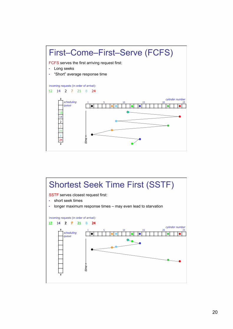
First–Come–First–Serve (FCFS) FCFS serves the first arriving request first: • Long seeks • “Short” average response time
time
cylinder number 1 5 10 15 20 25
12
incoming requests (in order of arrival):
14 2 7 21 8 24
scheduling queue
24
8
21
7
2
14
12
Shortest Seek Time First (SSTF) SSTF serves closest request first: • short seek times • longer maximum response times – may even lead to starvation
time
cylinder number 1 5 10 15 20 25
12
incoming requests (in order of arrival):
14 2 7 21 8 24
scheduling queue
24 8 21 7 2 14 12
21
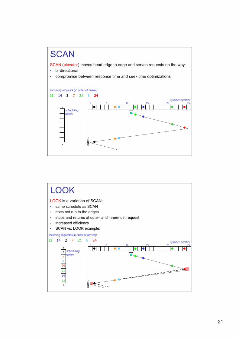
SCAN SCAN (elevator) moves head edge to edge and serves requests on the way: • bi-directional • compromise between response time and seek time optimizations
time
cylinder number 1 5 10 15 20 25
12
incoming requests (in order of arrival):
14 2 7 21 8 24
scheduling queue
24 8 21 7 2 14 12
LOOK LOOK is a variation of SCAN: • same schedule as SCAN • does not run to the edges • stops and returns at outer- and innermost request • increased efficiency • SCAN vs. LOOK example:
time
cylinder number 1 5 10 15 20 25
12
incoming requests (in order of arrival):
14 2 7 21 8 24
scheduling queue
24
8
21
7
2
14
12
22
Data Placement on Disk • Disk blocks can be assigned to files many ways, and
several schemes are designed for
optimized latency increased throughput
access pattern dependent
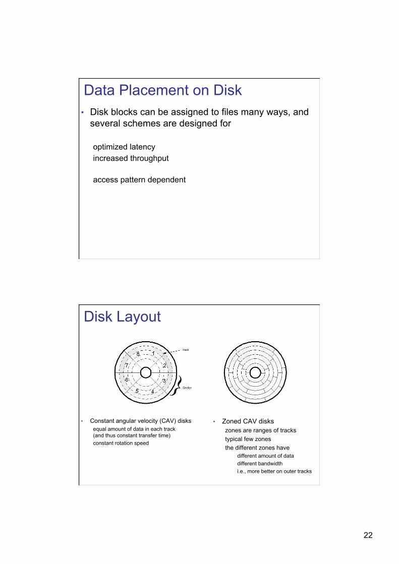
Disk Layout
• Constant angular velocity (CAV) disks equal amount of data in each track (and thus constant transfer time) constant rotation speed
• Zoned CAV disks zones are ranges of tracks typical few zones the different zones have
different amount of data different bandwidth i.e., more better on outer tracks
23
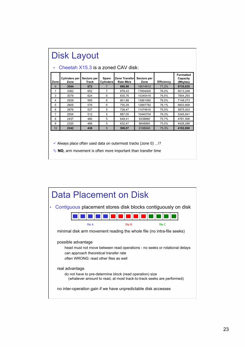
Disk Layout • Cheetah X15.3 is a zoned CAV disk:
Zone Cylinders per
Zone Sectors per
Track Spare
Cylinders Zone Transfer
Rate Mb/s Sectors per
Zone Efficiency
Formatted Capacity (Mbytes)
0 3544 672 7 890,98 19014912 77,2% 9735,635 1 3382 652 7 878,43 17604000 76,0% 9013,248 3 3079 624 6 835,76 15340416 76,5% 7854,293 4 2939 595 6 801,88 13961080 76,0% 7148,073 5 2805 576 6 755,29 12897792 78,1% 6603,669 6 2676 537 5 728,47 11474616 75,5% 5875,003 7 2554 512 5 687,05 10440704 76,3% 5345,641 8 2437 480 5 649,41 9338880 75,7% 4781,506 9 2325 466 5 632,47 8648960 75,5% 4428,268
10 2342 438 5 596,07 8188848 75,3% 4192,690
Always place often used data on outermost tracks (zone 0) …!?
NO, arm movement is often more important than transfer time
Data Placement on Disk • Contiguous placement stores disk blocks contiguously on disk
minimal disk arm movement reading the whole file (no intra-file seeks)
possible advantage head must not move between read operations - no seeks or rotational delays can approach theoretical transfer rate often WRONG: read other files as well
real advantage do not have to pre-determine block (read operation) size
(whatever amount to read, at most track-to-track seeks are performed)
no inter-operation gain if we have unpredictable disk accesses
file A file B file C
24
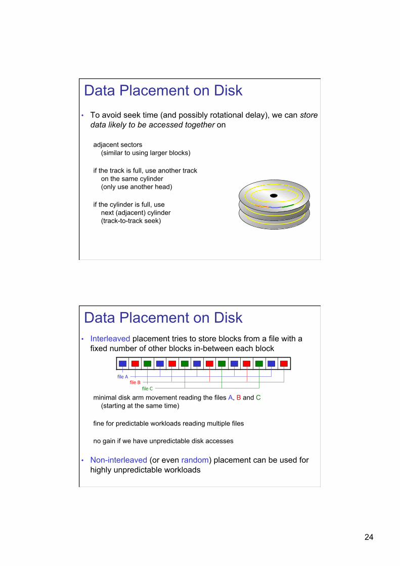
Data Placement on Disk • To avoid seek time (and possibly rotational delay), we can store
data likely to be accessed together on
adjacent sectors (similar to using larger blocks)
if the track is full, use another track on the same cylinder (only use another head)
if the cylinder is full, use next (adjacent) cylinder (track-to-track seek)
Data Placement on Disk • Interleaved placement tries to store blocks from a file with a
fixed number of other blocks in-between each block
minimal disk arm movement reading the files A, B and C (starting at the same time)
fine for predictable workloads reading multiple files
no gain if we have unpredictable disk accesses
• Non-interleaved (or even random) placement can be used for highly unpredictable workloads
file A file B
file C
25
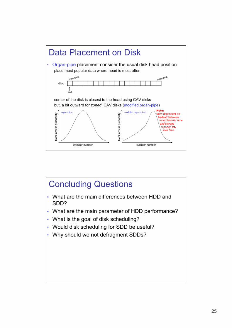
Data Placement on Disk • Organ-pipe placement consider the usual disk head position
place most popular data where head is most often
center of the disk is closest to the head using CAV disks but, a bit outward for zoned CAV disks (modified organ-pipe)
disk: innermost
outermost
head
bloc
k ac
cess
pro
babi
lity
cylinder number
bloc
k ac
cess
pro
babi
lity
cylinder number
organ-pipe: modified organ-pipe: Note: skew dependent on tradeoff between zoned transfer time and storage capacity vs. seek time
Concluding Questions • What are the main differences between HDD and
SDD? • What are the main parameter of HDD performance? • What is the goal of disk scheduling? • Would disk scheduling for SDD be useful? • Why should we not defragment SDDs?
26
Additional Material • Prefetching & Buffering • RAID systems
Prefetching • If we can predict the access pattern, one might speed up performance
using prefetching a video playout is often linear easy to predict access pattern
eases disk scheduling read larger amounts of data per request data in memory when requested – reducing page faults
• One simple (and efficient) way of doing prefetching is read-ahead: read more than the requested block into memory serve next read requests from buffer cache
• Another way of doing prefetching is double (multiple) buffering: read data into first buffer process data in first buffer and at the same time read data into second buffer process data in second buffer and at the same time read data into first buffer etc.
27
process data
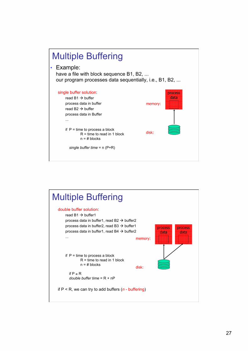
Multiple Buffering • Example:
have a file with block sequence B1, B2, ... our program processes data sequentially, i.e., B1, B2, ...
single buffer solution: read B1 buffer process data in buffer read B2 buffer process data in Buffer ...
if P = time to process a block R = time to read in 1 block n = # blocks
single buffer time = n (P+R)
disk:
memory:
Multiple Buffering double buffer solution:
read B1 buffer1 process data in buffer1, read B2 buffer2 process data in buffer2, read B3 buffer1 process data in buffer1, read B4 buffer2 ...
if P = time to process a block R = time to read in 1 block n = # blocks
if P ≥ R double buffer time = R + nP
if P < R, we can try to add buffers (n - buffering)
process data
disk:
memory:
process data
28
Pentium 4 Processor
registers
cache(s)
I/O controller
hub
memory controller
hub
RDRAM RDRAM
RDRAM RDRAM
PCI slots PCI slots PCI slots
network card
disk
file system communication system
application
file system communication system
application
disk network card
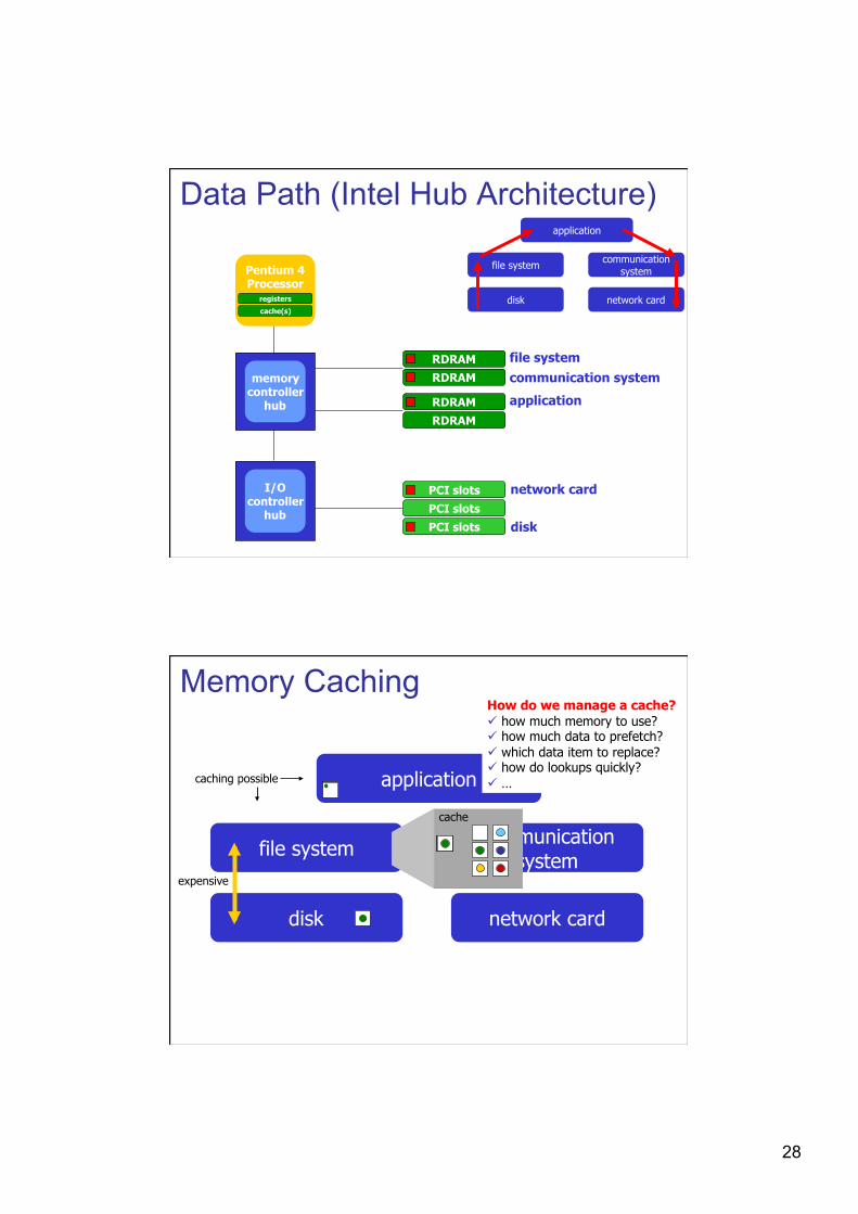
Data Path (Intel Hub Architecture)
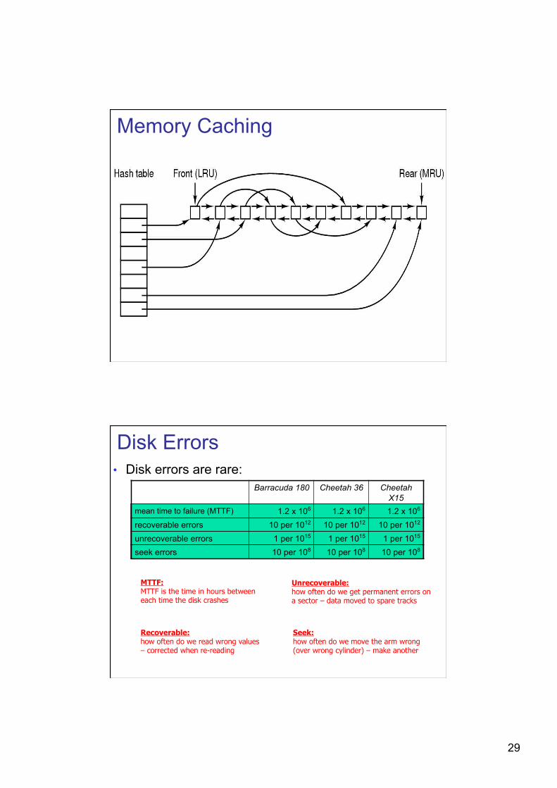
Memory Caching
communication system
application
disk network card
expensive
file system
cache
caching possible
How do we manage a cache? how much memory to use? how much data to prefetch? which data item to replace? how do lookups quickly? …
29
Memory Caching
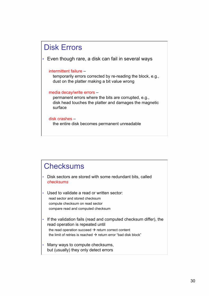
Disk Errors • Disk errors are rare:
Barracuda 180 Cheetah 36 Cheetah X15
mean time to failure (MTTF) 1.2 x 10⁶ 1.2 x 10⁶ 1.2 x 10⁶
recoverable errors 10 per 1012 10 per 1012 10 per 1012 unrecoverable errors 1 per 1015 1 per 1015 1 per 1015 seek errors 10 per 108 10 per 108 10 per 108
MTTF: MTTF is the time in hours between each time the disk crashes
Recoverable: how often do we read wrong values – corrected when re-reading
Unrecoverable: how often do we get permanent errors on a sector – data moved to spare tracks
Seek: how often do we move the arm wrong (over wrong cylinder) – make another
30
Disk Errors • Even though rare, a disk can fail in several ways
intermittent failure – temporarily errors corrected by re-reading the block, e.g., dust on the platter making a bit value wrong
media decay/write errors – permanent errors where the bits are corrupted, e.g., disk head touches the platter and damages the magnetic surface
disk crashes – the entire disk becomes permanent unreadable
Checksums • Disk sectors are stored with some redundant bits, called
checksums
• Used to validate a read or written sector: read sector and stored checksum compute checksum on read sector compare read and computed checksum
• If the validation fails (read and computed checksum differ), the read operation is repeated until the read operation succeed return correct content the limit of retries is reached return error “bad disk block”
• Many ways to compute checksums, but (usually) they only detect errors
31
Disk Failure Models
• Our Seagate disks have a MTTF of ~130 years (at this time ~50 % of the disks are damaged), but
many disks fail during the first months (production errors)
if no production errors, disks will probably work many years
old disks have again a larger probability of failure due to accumulated effects of dust, etc.
Crash Recovery • The most serious type of errors are disk crashes, e.g.,
head have touched platter and is damaged platters are out of position ...
• Usually, no way to restore data unless we have a backup on another medium, e.g., tape, mirrored disk, etc.
• A number of schemes have been developed to reduce the probability of data loss during permanent disk errors usually using an extended parity check most known are the Redundant Array of Independent Disks (RAID)
strategies
32
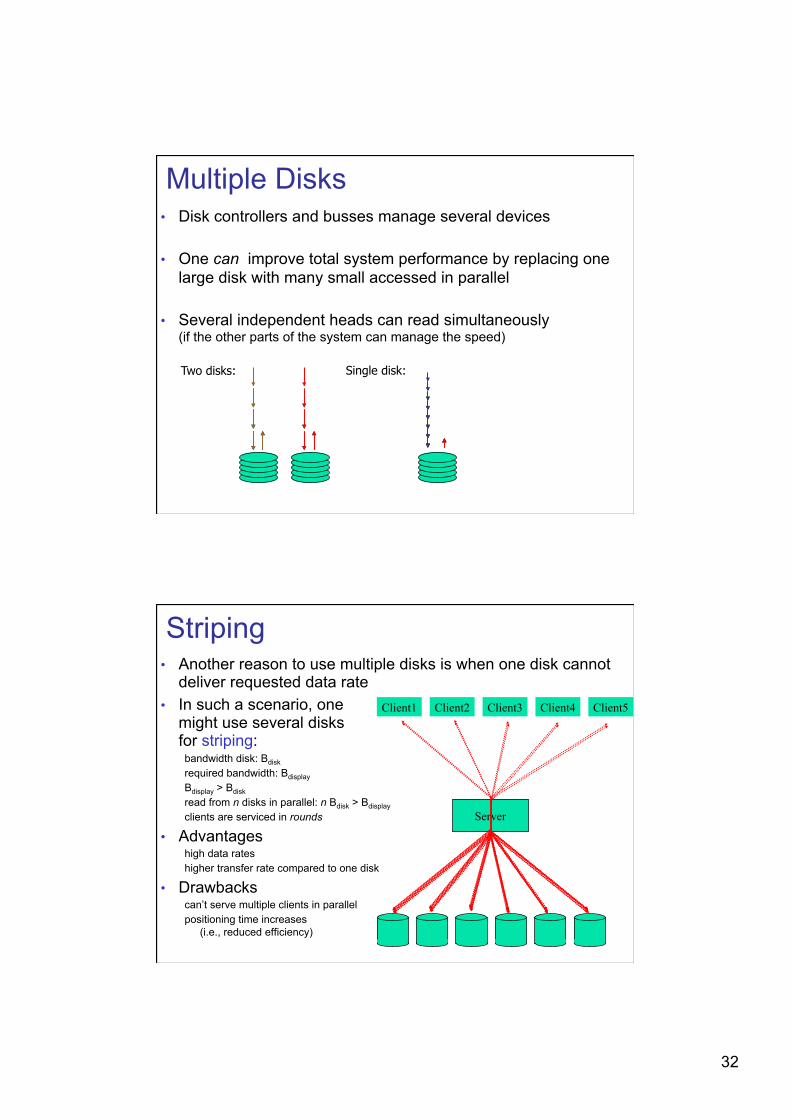
Multiple Disks • Disk controllers and busses manage several devices
• One can improve total system performance by replacing one large disk with many small accessed in parallel
• Several independent heads can read simultaneously (if the other parts of the system can manage the speed)
Single disk: Two disks:
Client1 Client2 Client3 Client4 Client5
Server
Striping • Another reason to use multiple disks is when one disk cannot
deliver requested data rate • In such a scenario, one
might use several disks for striping:
bandwidth disk: Bdisk required bandwidth: Bdisplay Bdisplay > Bdisk read from n disks in parallel: n Bdisk > Bdisplay
clients are serviced in rounds
• Advantages high data rates higher transfer rate compared to one disk
• Drawbacks can’t serve multiple clients in parallel positioning time increases
(i.e., reduced efficiency)
33
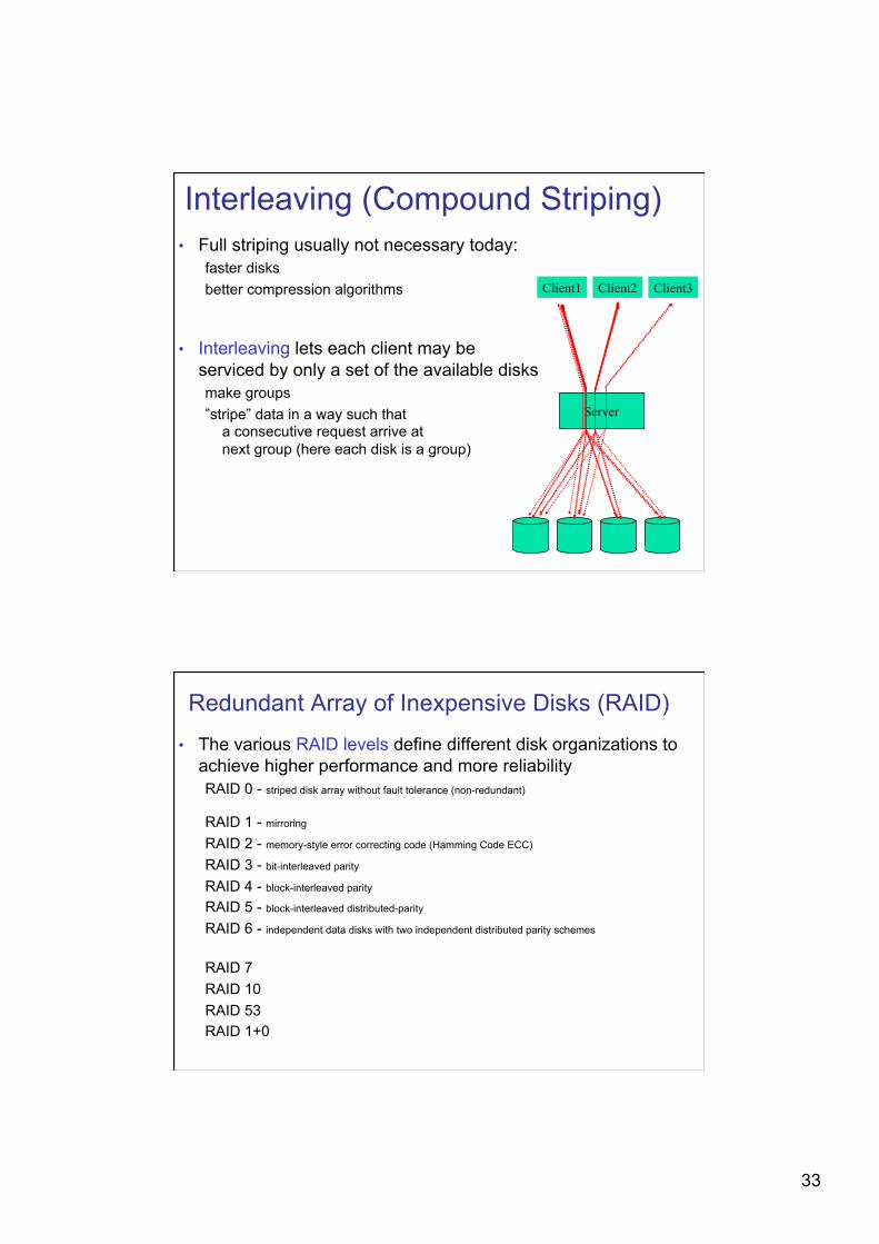
Interleaving (Compound Striping) • Full striping usually not necessary today:
faster disks better compression algorithms
• Interleaving lets each client may be serviced by only a set of the available disks make groups ”stripe” data in a way such that
a consecutive request arrive at next group (here each disk is a group)
Client1 Client2 Client3
Server
Redundant Array of Inexpensive Disks (RAID) • The various RAID levels define different disk organizations to
achieve higher performance and more reliability RAID 0 - striped disk array without fault tolerance (non-redundant)
RAID 1 - mirroring
RAID 2 - memory-style error correcting code (Hamming Code ECC)
RAID 3 - bit-interleaved parity
RAID 4 - block-interleaved parity RAID 5 - block-interleaved distributed-parity
RAID 6 - independent data disks with two independent distributed parity schemes
RAID 7 RAID 10 RAID 53 RAID 1+0
34
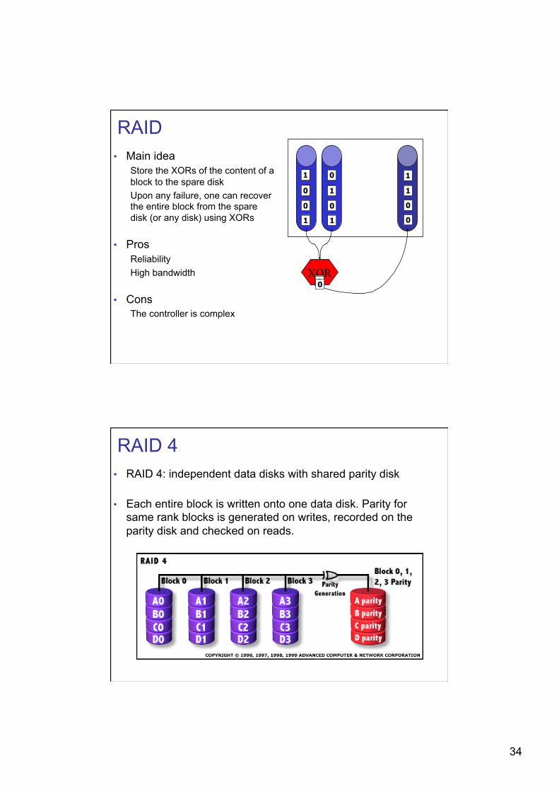
RAID • Main idea
Store the XORs of the content of a block to the spare disk Upon any failure, one can recover the entire block from the spare disk (or any disk) using XORs
• Pros Reliability High bandwidth
• Cons The controller is complex
XOR
1
0
0
1
0
1
0
1
1
1
0
0
1
1 0
0 1
1
0 0
0
1 1
0
RAID 4 • RAID 4: independent data disks with shared parity disk
• Each entire block is written onto one data disk. Parity for same rank blocks is generated on writes, recorded on the parity disk and checked on reads.
35
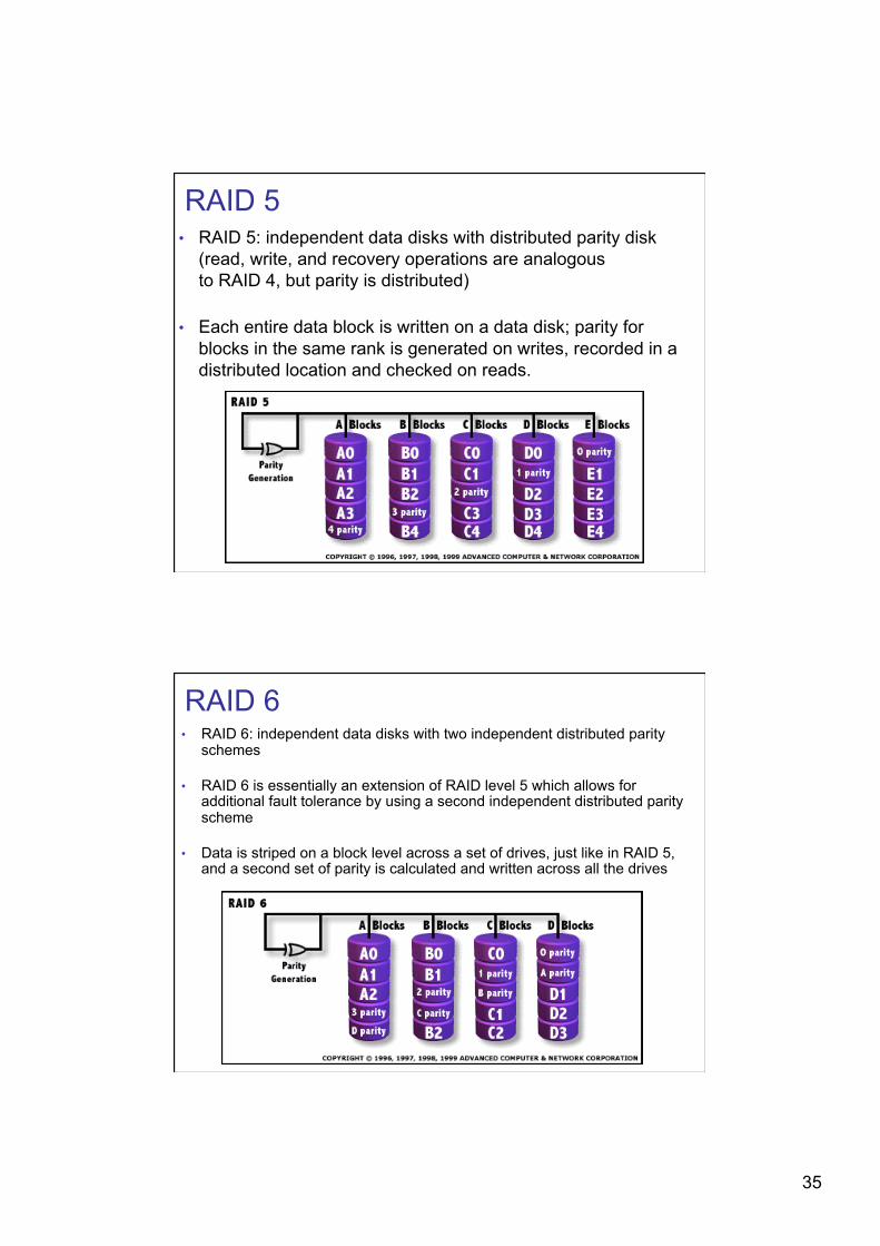
RAID 5 • RAID 5: independent data disks with distributed parity disk
(read, write, and recovery operations are analogous to RAID 4, but parity is distributed)
• Each entire data block is written on a data disk; parity for blocks in the same rank is generated on writes, recorded in a distributed location and checked on reads.
• RAID 6: independent data disks with two independent distributed parity schemes
• RAID 6 is essentially an extension of RAID level 5 which allows for additional fault tolerance by using a second independent distributed parity scheme
• Data is striped on a block level across a set of drives, just like in RAID 5, and a second set of parity is calculated and written across all the drives
RAID 6
36
RAID 6 • In general, we can add several redundancy disks to be able do
deal with several simultaneous disk crashes
• Many different strategies based on different EECs, e.g.,:
Read-Solomon Code (or derivates): corrects n simultaneous disk crashes using n parity disks a bit more expensive parity calculations compared to XOR
Hamming Code: corrects 2 disk failures using 2K – 1 disks where k disks are parity disks
and 2K – k – 1 the parity disks are calculated using the data disks determined by the hamming
code, i.e., a k x (2K – 1) matrix of 0’s and 1’s representing the 2K – 1 numbers written binary except 0
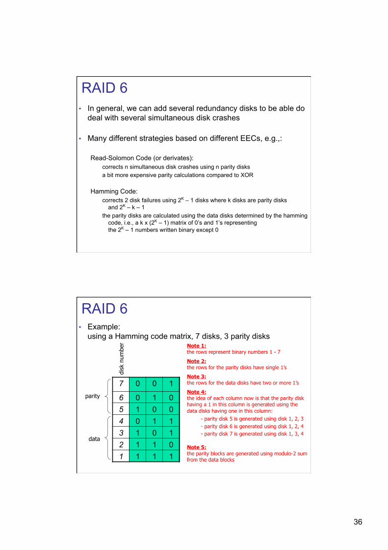
RAID 6 • Example:
using a Hamming code matrix, 7 disks, 3 parity disks
7 0 0 1
6 0 1 0 5 1 0 0 4 0 1 1 3 1 0 1 2 1 1 0 1 1 1 1
disk
num
ber
parity
data
Note 1: the rows represent binary numbers 1 - 7
Note 2: the rows for the parity disks have single 1’s
Note 3: the rows for the data disks have two or more 1’s
Note 4: the idea of each column now is that the parity disk having a 1 in this column is generated using the data disks having one in this column:
- parity disk 5 is generated using disk 1, 2, 3
- parity disk 6 is generated using disk 1, 2, 4
- parity disk 7 is generated using disk 1, 3, 4
Note 5: the parity blocks are generated using modulo-2 sum from the data blocks
37
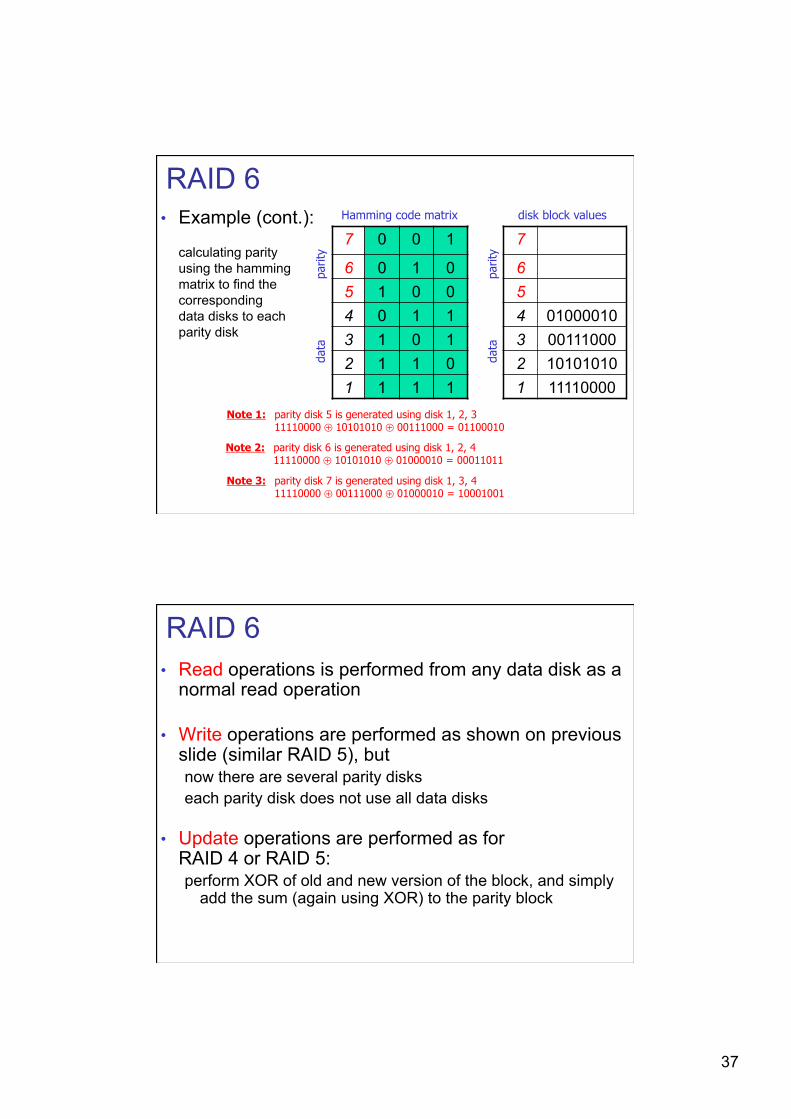
RAID 6 • Example (cont.):
calculating parity using the hamming matrix to find the corresponding data disks to each parity disk
7 0 0 1
6 0 1 0 5 1 0 0 4 0 1 1 3 1 0 1 2 1 1 0 1 1 1 1
parit
y da
ta
7 10001001
6 00011011 5 01100010 4 01000010 3 00111000 2 10101010 1 11110000
parit
y da
ta
Hamming code matrix disk block values
Note 1: parity disk 5 is generated using disk 1, 2, 3 11110000 ⊕ 10101010 ⊕ 00111000 = 01100010
Note 2: parity disk 6 is generated using disk 1, 2, 4 11110000 ⊕ 10101010 ⊕ 01000010 = 00011011
Note 3: parity disk 7 is generated using disk 1, 3, 4 11110000 ⊕ 00111000 ⊕ 01000010 = 10001001
RAID 6 • Read operations is performed from any data disk as a
normal read operation
• Write operations are performed as shown on previous slide (similar RAID 5), but now there are several parity disks each parity disk does not use all data disks
• Update operations are performed as for RAID 4 or RAID 5: perform XOR of old and new version of the block, and simply
add the sum (again using XOR) to the parity block
38
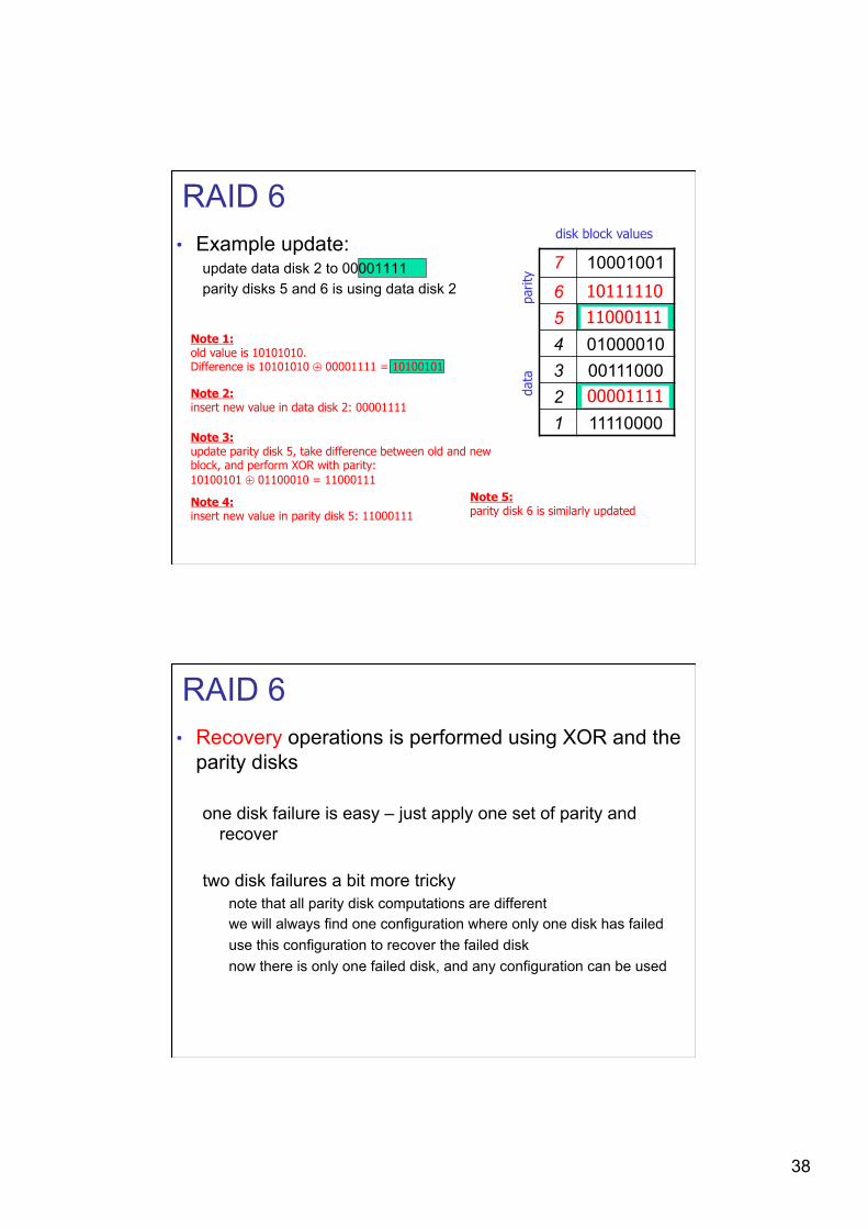
RAID 6 • Example update:
update data disk 2 to 00001111 parity disks 5 and 6 is using data disk 2
7 10001001 6 00011011 5 01100010 4 01000010 3 00111000 2 10101010 1 11110000
parit
y da
ta
disk block values
Note 1: old value is 10101010. Difference is 10101010 ⊕ 00001111 = 10100101
Note 2: insert new value in data disk 2: 00001111
00001111
Note 3: update parity disk 5, take difference between old and new block, and perform XOR with parity: 10100101 ⊕ 01100010 = 11000111
11000111
Note 4: insert new value in parity disk 5: 11000111
Note 5: parity disk 6 is similarly updated
10111110
RAID 6 • Recovery operations is performed using XOR and the
parity disks
one disk failure is easy – just apply one set of parity and recover
two disk failures a bit more tricky note that all parity disk computations are different we will always find one configuration where only one disk has failed use this configuration to recover the failed disk now there is only one failed disk, and any configuration can be used
39
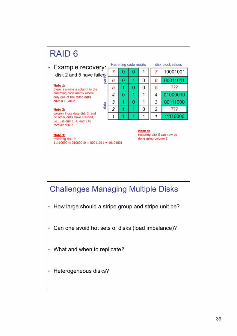
RAID 6 • Example recovery:
disk 2 and 5 have failed 7 0 0 1
6 0 1 0 5 1 0 0 4 0 1 1 3 1 0 1 2 1 1 0 1 1 1 1
parit
y da
ta
7 10001001
6 00011011 5 01100001 4 01000010 3 00111000 2 10101001 1 11110000
Hamming code matrix disk block values
???
???
Note 1: there is always a column in the hamming code matrix where only one of the failed disks have a 1- value
Note 2: column 2 use data disk 2, and no other disks have crashed, i.e., use disk 1, 4, and 6 to recover disk 2
Note 3: restoring disk 2: 11110000 ⊕ 01000010 ⊕ 00011011 = 10101001
Note 4: restoring disk 5 can now be done using column 1
Challenges Managing Multiple Disks
• How large should a stripe group and stripe unit be?
• Can one avoid hot sets of disks (load imbalance)?
• What and when to replicate?
• Heterogeneous disks?
40
Summary • The main bottleneck is disk I/O performance due to disk
mechanics: seek time and rotational delays
• Much work has been performed to optimize disks performance Many algorithms trying to minimize seek overhead
(most existing systems uses a SCAN derivate) use large block sizes or read many continuous blocks prefetch data from disk to memory striping might not be necessary on new disks (at least not on all disks) memory caching can save disk I/Os
• World today more complicated (both different access patterns and unknown disk characteristics) new disks are “smart”, we cannot fully control the device


