Evaluation of CT Saturation Impact for Various 87L Applications
Zhihan Xu (GE Digital Energy), Matt Proctor (GE Digital Energy)
Ilia Voloh (GE Digital Energy), Mike Lara (SNC-Lavalin)
Abstract — This paper will explore requirements for the line current differential function (87L) with
regards to the impact of current transformer (CT) saturation for various 87L applications. Percent
differential elements typically cope with CT saturation using proper restraint but also have algorithms
designed to tolerate CT errors including CT saturation. How to use restraint settings and these algorithms
properly for a given application is not an easy task and is not understood well by protection engineers.
Therefore, how to estimate reliability of the differential during CT saturation conditions is not an easy
task at all.
The paper will first explain the general knowledge of CT fundamental and saturation. Secondly, the paper
will investigate security and dependability aspects of the 87L during CT saturation caused by internal and
external faults. Then, techniques that have been used or can be used in 87L to reduce CT requirement and
improve relay security are discussed. A practical analysis tool is presented for different applications,
including breaker-and-a-half or ring configurations, to analyze reliability of 87L during CT saturation,
evaluate the differential relay security, investigate the effect of adjusting 87L settings, choose the proper
size of CT and examine the possibility of reducing CT requirement. A more accuracy method is described
as well to estimate the CT time to saturation.
Index Terms —Line Differential Relay, Security and Dependability, CT Saturation, Time to Saturation
I. CT FUNDAMENTALS
Current Transformer (CT) is simply a transformer designed for the specific application of
converting primary current to a secondary current for measurement, protection and control
purposes [1], [2]. Apparently, a CT is like any other kind of transformer, which consists of two
windings magnetically coupled by the flux in a saturable steel core. A time varying voltage
applied to one winding produces magnetic flux in the core, which induces the voltage in the
second winding to deliver the secondary current. The transformer draws an exciting current to
keep the core excited [3]. Similarly, CT’s experience copper losses, core losses, eddy current
losses and leakage flux. So the secondary current of a CT is not a perfectly true replica of the
primary current in magnitude and there may exist a small phase shift.
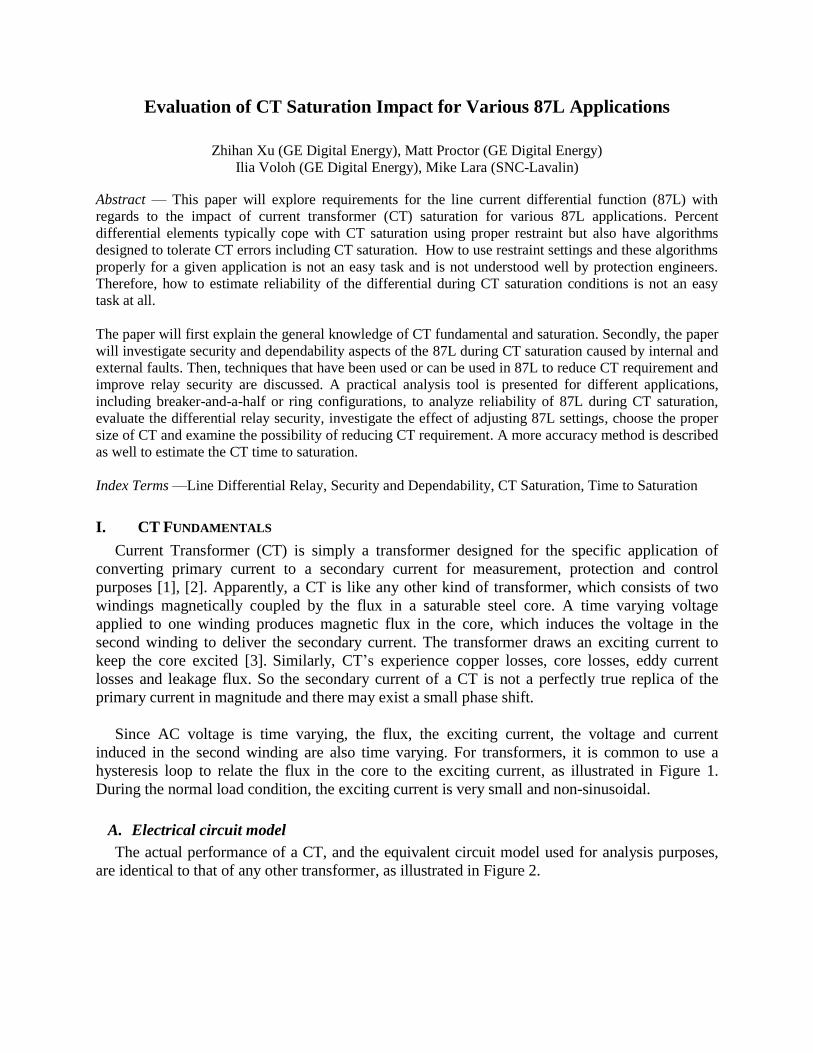
Since AC voltage is time varying, the flux, the exciting current, the voltage and current
induced in the second winding are also time varying. For transformers, it is common to use a
hysteresis loop to relate the flux in the core to the exciting current, as illustrated in Figure 1.
During the normal load condition, the exciting current is very small and non-sinusoidal.
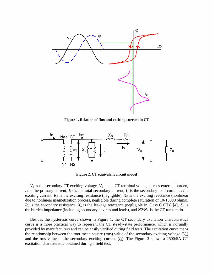
A. Electrical circuit model
The actual performance of a CT, and the equivalent circuit model used for analysis purposes,
are identical to that of any other transformer, as illustrated in Figure 2.
veφ
φ
iφ
ie
Figure 1. Relation of flux and exciting current in CT
N1 N2
IP IST
ISIEVs XE RE VB
XS RS
ZB
Ideal CT
Figure 2. CT equivalent circuit model
VS is the secondary CT exciting voltage, VB is the CT terminal voltage across external burden,
IP is the primary current, IST is the total secondary current, IS is the secondary load current, IE is
exciting current, RE is the exciting resistance (negligible), XE is the exciting reactance (nonlinear
due to nonlinear magnetization process, negligible during complete saturation or 10-10000 ohms),
RS is the secondary resistance, XS is the leakage reactance (negligible in Class C CTs) [4], ZB is
the burden impedance (including secondary devices and leads), and N2/N1 is the CT turns ratio.
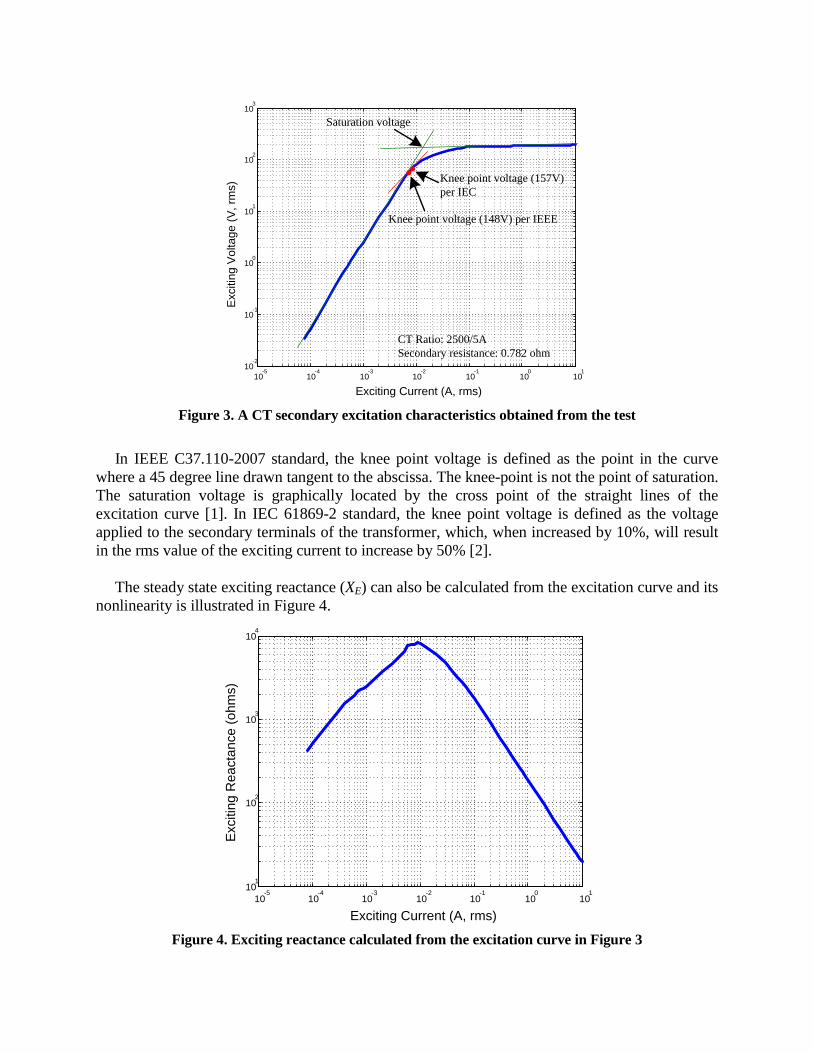
Besides the hysteresis curve shown in Figure 1, the CT secondary excitation characteristics
curve is a more practical way to represent the CT steady-state performance, which is normally
provided by manufacturers and can be easily verified during field tests. The excitation curve maps
the relationship between the root-mean-square (rms) value of the secondary exciting voltage (VS)
and the rms value of the secondary exciting current (IE). The Figure 3 shows a 2500:5A CT
excitation characteristic obtained during a field test.
10-5
10-4
10-3
10-2
10-1
100
101
10-2
10-1
100
101
102
103
Exciting Current (A, rms)
Excitin
g V
olta
ge
(V
, rm
s)
Knee point voltage (148V) per IEEE
Saturation voltage
CT Ratio: 2500/5A
Secondary resistance: 0.782 ohm
Knee point voltage (157V)
per IEC
Figure 3. A CT secondary excitation characteristics obtained from the test
In IEEE C37.110-2007 standard, the knee point voltage is defined as the point in the curve
where a 45 degree line drawn tangent to the abscissa. The knee-point is not the point of saturation.
The saturation voltage is graphically located by the cross point of the straight lines of the
excitation curve [1]. In IEC 61869-2 standard, the knee point voltage is defined as the voltage
applied to the secondary terminals of the transformer, which, when increased by 10%, will result
in the rms value of the exciting current to increase by 50% [2].
The steady state exciting reactance (XE) can also be calculated from the excitation curve and its
nonlinearity is illustrated in Figure 4.
10-5
10-4
10-3
10-2
10-1
100
101
101
102
103
104
Exciting Current (A, rms)
Excitin
g R
ea
cta
nce
(o
hm
s)
Figure 4. Exciting reactance calculated from the excitation curve in Figure 3
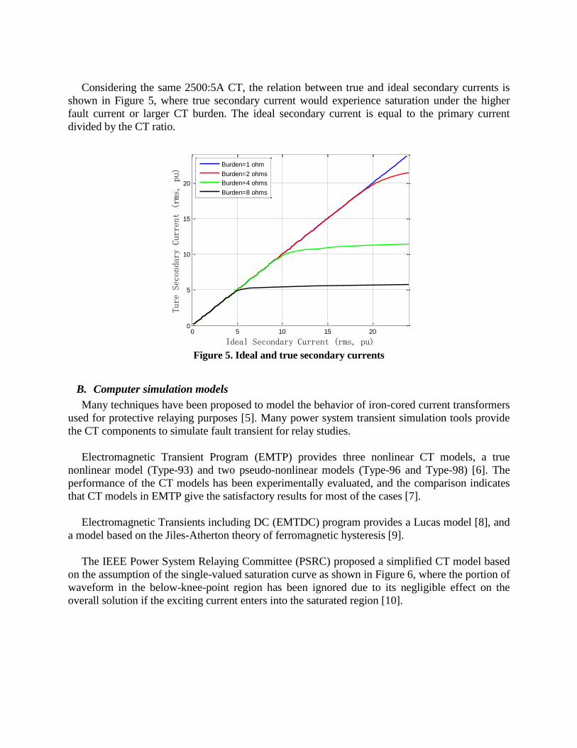
Considering the same 2500:5A CT, the relation between true and ideal secondary currents is
shown in Figure 5, where true secondary current would experience saturation under the higher
fault current or larger CT burden. The ideal secondary current is equal to the primary current
divided by the CT ratio.
Figure 5. Ideal and true secondary currents
B. Computer simulation models
Many techniques have been proposed to model the behavior of iron-cored current transformers
used for protective relaying purposes [5]. Many power system transient simulation tools provide
the CT components to simulate fault transient for relay studies.
Electromagnetic Transient Program (EMTP) provides three nonlinear CT models, a true
nonlinear model (Type-93) and two pseudo-nonlinear models (Type-96 and Type-98) [6]. The
performance of the CT models has been experimentally evaluated, and the comparison indicates
that CT models in EMTP give the satisfactory results for most of the cases [7].
Electromagnetic Transients including DC (EMTDC) program provides a Lucas model [8], and
a model based on the Jiles-Atherton theory of ferromagnetic hysteresis [9].
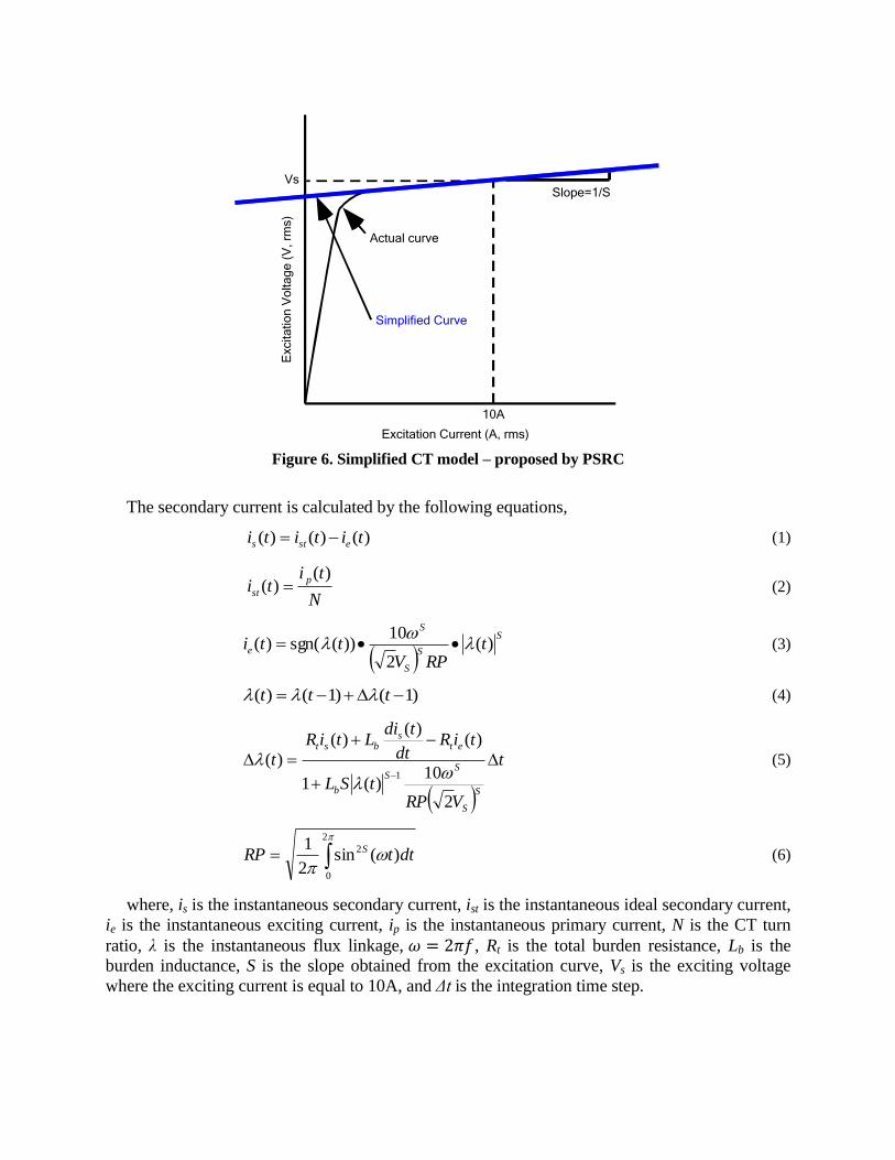
The IEEE Power System Relaying Committee (PSRC) proposed a simplified CT model based
on the assumption of the single-valued saturation curve as shown in Figure 6, where the portion of
waveform in the below-knee-point region has been ignored due to its negligible effect on the
overall solution if the exciting current enters into the saturated region [10].
0 5 10 15 200
5
10
15
20
Ideal Secondary Current (rms, pu)
Ture Secondary Current (rms, pu)
Burden=1 ohm
Burden=2 ohms
Burden=4 ohms
Burden=8 ohms
Actual curve
Simplified Curve
10A
Excitation Current (A, rms)
Excita
tio
n V
olta
ge
(V
, rm
s)
VsSlope=1/S
Figure 6. Simplified CT model – proposed by PSRC
The secondary current is calculated by the following equations,
)()()( tititi ests (1)
N
titi
p
st
)()( (2)
S
S
S
S
e tRPV
tti )(2
10))(sgn()(
(3)
)1()1()( ttt (4)
t
VRPtSL
tiRdt
tdiLtiR
t
S
S
SS
b
ets
bst
2
10)(1
)()(
)(
)(1
(5)
2
0
2 )(sin2
1dttRP S
(6)
where, is is the instantaneous secondary current, ist is the instantaneous ideal secondary current,
ie is the instantaneous exciting current, ip is the instantaneous primary current, N is the CT turn
ratio, λ is the instantaneous flux linkage, 𝜔 = 2𝜋𝑓, Rt is the total burden resistance, Lb is the
burden inductance, S is the slope obtained from the excitation curve, Vs is the exciting voltage
where the exciting current is equal to 10A, and Δt is the integration time step.

An Excel spreadsheet has been developed by the IEEE PSRC for the purpose of easy
application [11].
This IEEE PSRC CT model has been verified by multiple parties [10] and validated in a high
current laboratory [12]. The laboratory obtained saturated CT waveforms agreed to the IEEE
PSRC CT model waveforms very closely. Therefore, this simplified CT model can be used for CT
saturation modeling and is used in this paper as well.
II. CT SATURATION
When the exciting voltage is greater than the knee voltage in the excitation curve, the CT
enters the saturated region, where the exciting current (IE) is no longer negligible. Therefore, the
ratio error (IE/IS×100%) of the exciting current to the secondary current increases and the
secondary current (IS) is distorted, not being sinusoidal anymore.
A. AC saturation
AC saturation, also called steady state saturation, is caused by the symmetrical current with no
DC component. A set of AC saturation examples is shown in the figure below.
Figure 7. Examples of AC saturation
In order to avoid ac saturation, the secondary saturation voltage, VX, must satisfy the following
equation.
SSX ZIV (7)
where, IS is the primary current divided by the turns ratio, and ZS is the total secondary burden
(RS + XS + ZB). It can be observed that the AC saturation may be caused by the higher primary
current, lower ratio CT (such as ground CT), or larger CT burden (long lead length, and/or small
AWG wire gage). Therefore, the AC saturation can be avoided by properly increasing the CT
saturation voltage, CT ratio, or decreasing CT burden.
0.015 0.02 0.025 0.03 0.035 0.04 0.045 0.05-1.5
-1
-0.5
0
0.5
1
1.5
Time (s)
Current (pu of fault)
Saturated Secondary
Current (15-65kA)
Ratio Current
CT Ratio: 800/5
Burden: 2 ohms
Vs@10A: 303 V
DC offset: 0%
In real applications, a commonly used rule of thumb is to select a CT with the voltage rating of
a Class C CT at least twice that required for the maximum steady state symmetrical fault current
[1].
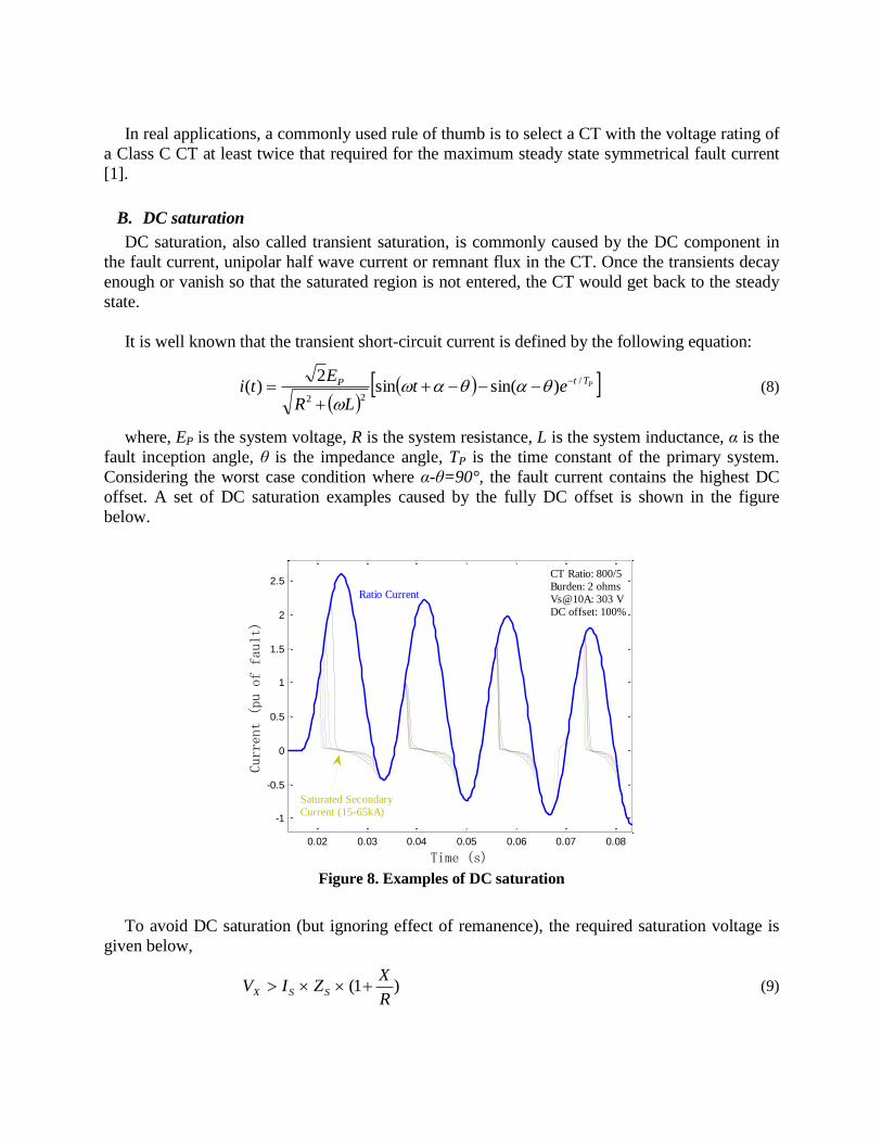
B. DC saturation
DC saturation, also called transient saturation, is commonly caused by the DC component in
the fault current, unipolar half wave current or remnant flux in the CT. Once the transients decay
enough or vanish so that the saturated region is not entered, the CT would get back to the steady
state.
It is well known that the transient short-circuit current is defined by the following equation:
PTtP et
LR
Eti
/
22)sin(sin
2)(
(8)
where, EP is the system voltage, R is the system resistance, L is the system inductance, α is the
fault inception angle, θ is the impedance angle, TP is the time constant of the primary system.
Considering the worst case condition where α-θ=90°, the fault current contains the highest DC
offset. A set of DC saturation examples caused by the fully DC offset is shown in the figure
below.
Figure 8. Examples of DC saturation
To avoid DC saturation (but ignoring effect of remanence), the required saturation voltage is
given below,
)1(R
XZIV SSX (9)
0.02 0.03 0.04 0.05 0.06 0.07 0.08
-1
-0.5
0
0.5
1
1.5
2
2.5
Time (s)
Current (pu of fault)
Saturated Secondary
Current (15-65kA)
Ratio Current
CT Ratio: 800/5
Burden: 2 ohms
Vs@10A: 303 V
DC offset: 100%

where, X/R is the primary system X/R ratio. Comparing Eq. (7) with Eq. (9), it can be found
that the knee point voltage to avoid dc saturation must be (1+X/R) times that required for avoiding
AC saturation.
C. Contributing factors to CT saturation
Regarding a specified CT, mostly, there are four factors which contribute to CT saturation:
High primary fault current
Excessive secondary burden
Heavy DC offset in current
Large percent remanence
Apparently, the increase in primary fault current will increase secondary current, sequentially,
increase exciting voltage, enter into the saturated region and significantly increase exciting
current. As a result, the secondary current is greatly reduced and distorted. Both Figure 7 and
Figure 8 show the saturated secondary currents.
Larger CT burdens increase exciting voltage under the same fault current, and increase
exciting current. Then CT is more likely to saturate.
As indicated by the analysis of Eq. (8), the maximum DC component of a fault occurs when
the instantaneous voltage is zero. Then the DC component starts decaying according to the time
constant of the primary power system. The larger time constant will result in the longer decaying
process, and then longer CT saturation period.
Remanence, also called remanent flux or residual flux, is the magnetic flux that is retained in
the magnetic circuit after the removal of the excitation. Remanence may remain in either positive
or negative direction. When the CT is subject to subsequent fault current again, the flux changes
will start from the remanent value. Then the shifted remanence may worsen the transient response
by pushing the core into deeper saturation within shorter time if the remanence and instantaneous
flux have the same direction, or improve the transient response by keeping the core away from the
deeper saturation if the remanence and instantaneous flux have the opposite direction.
III. IMPACT OF CT SATURATON ON 87L
The Eq. (9) describes the criterion of sizing CT to avoid DC saturation. However, it is not
always practical or possible to satisfy for different applications. In practice, it is rarely possible to
completely prevent the occurring of CT saturation for different fault events.
The distorted secondary current caused by CT saturation would inevitably affect the
performance of current-based protection elements, such as overcurrent, directional overcurrent,
distance, differential and others. The performance requirements of CT for various protection
applications have been introduced in [13], [14]. This section will discuss the impact of CT
saturation on line current differential relays.

A. Effect on current phasor estimation
Most of current-based protection functions are using the current phasor. This section will
discuss the effect of CT saturation on one of mostly used phasor estimation techniques, Discrete
Fourier Transform (DFT). It should be mentioned that in the real implementation of relays, some
filtering techniques may be applied to remove DC decaying transients, or the cosine filter is used
for phasor estimation, however, these techniques are not considered in this paper.
The phasor of the secondary current is calculated by DFT as below,
1
0
/)5.0(22 NC
p
NCpi
SS eiNC
I
1
0
/)5.0(2)(2 NC
p
NCpi
EST eiiNC
1
0
/)5.0(21
0
/)5.0(2 22 NC
p
NCpi
E
NC
p
NCpi
ST eiNC
eiNC
(10)
1
0
/)5.0(22 NC
p
NCpi
EST eiNC
I
EST II
where, IS, IST and IE are the phasors of the true secondary current, ideal secondary current and
exciting current, iS, iST and iE are the instantaneous currents, NC is the amount of samples per
cycle.
It can be found that an error exists between true and ideal current phasors caused by the
exciting current (iE). Since there are many factors affecting the saturation process and the exciting
current is a quite nonlinear quantity, it is hard to give an accurate and definite analysis based on
Eq. (10). Therefore, some assumptions are applied for further analysis,
Without saturation, the true and ideal currents have the exact same samples.
During saturation, the true current samples are zero.
Saturation is repeated each half cycle with the same pattern.
There is no dc offset.
The time to saturation longer than half cycle is not considered since the differential relays normally operate at the high speed.
An example of saturated current with assumptions is shown below, where the time to
saturation is around 2.86 ms at 60 Hz.
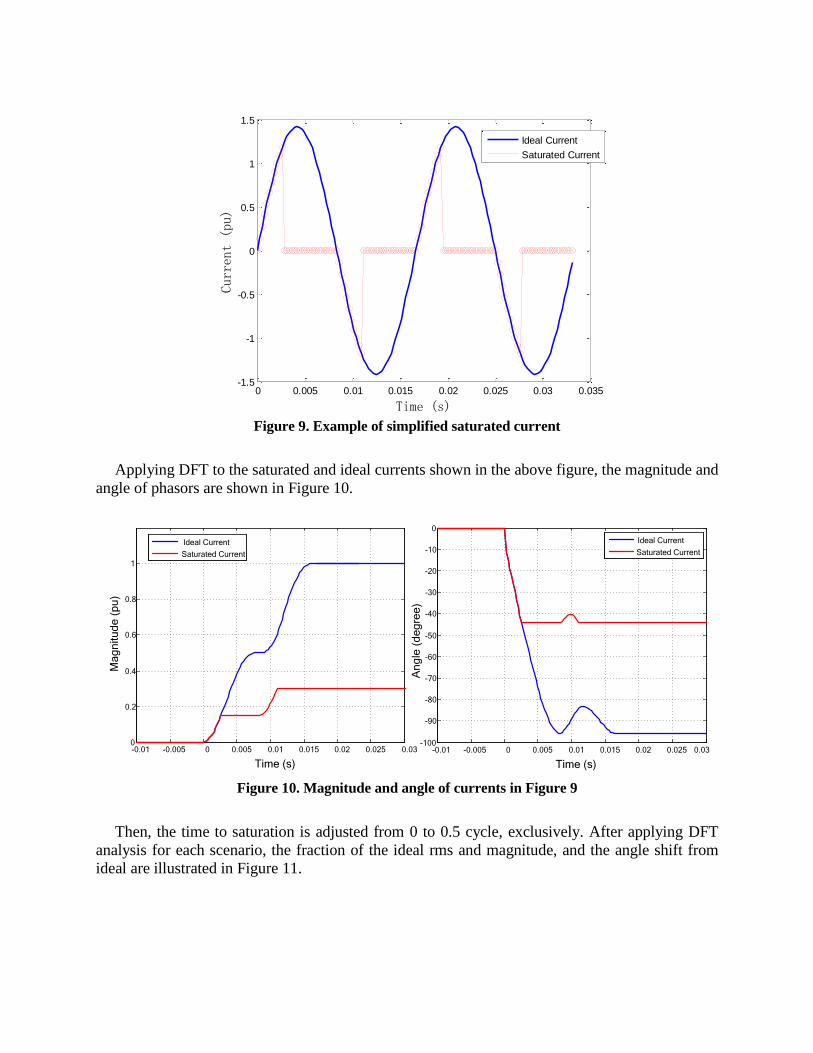
Figure 9. Example of simplified saturated current
Applying DFT to the saturated and ideal currents shown in the above figure, the magnitude and
angle of phasors are shown in Figure 10.
-0.01 -0.005 0 0.005 0.01 0.015 0.02 0.025 0.030
0.2
0.4
0.6
0.8
1
Time (s)
Ma
gn
itu
de
(p
u)
Ideal Current
Saturated Current
-0.01 -0.005 0 0.005 0.01 0.015 0.02 0.025 0.03-100
-90
-80
-70
-60
-50
-40
-30
-20
-10
0
Time (s)
An
gle
(d
eg
ree
)
Ideal Current
Saturated Current
Figure 10. Magnitude and angle of currents in Figure 9
Then, the time to saturation is adjusted from 0 to 0.5 cycle, exclusively. After applying DFT
analysis for each scenario, the fraction of the ideal rms and magnitude, and the angle shift from
ideal are illustrated in Figure 11.
0 0.005 0.01 0.015 0.02 0.025 0.03 0.035-1.5
-1
-0.5
0
0.5
1
1.5
Time (s)
Current (pu)
Ideal Current
Saturated Current
Ma
gn
itu
de
(α
, p
u o
f id
ea
l)A
ng
le S
hift fro
m Id
ea
l (β, d
eg
ree
, lea
din
g)
RM
S (
pu
of id
ea
l)
5 10 15 20 25 300
0.2
0.4
0.6
0.8
1
Time to saturation (1/64 cyc)
5 10 15 20 25 300
20
40
60
80
100
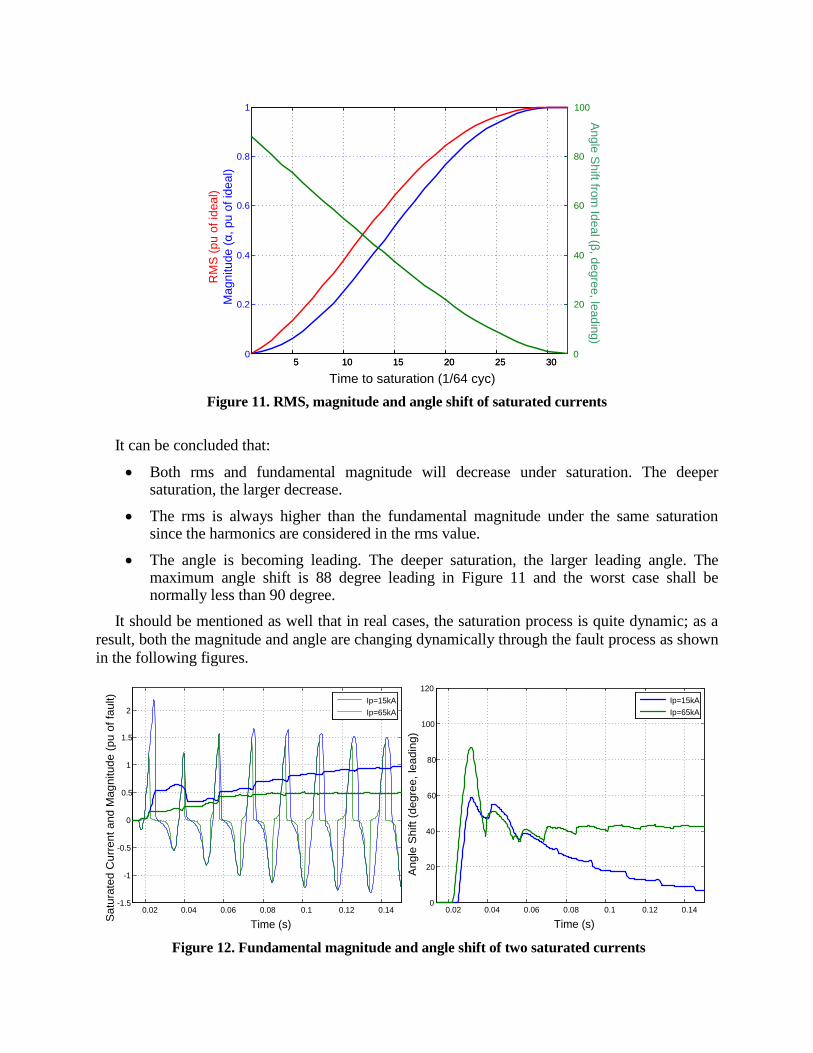
Figure 11. RMS, magnitude and angle shift of saturated currents
It can be concluded that:
Both rms and fundamental magnitude will decrease under saturation. The deeper saturation, the larger decrease.
The rms is always higher than the fundamental magnitude under the same saturation since the harmonics are considered in the rms value.
The angle is becoming leading. The deeper saturation, the larger leading angle. The maximum angle shift is 88 degree leading in Figure 11 and the worst case shall be normally less than 90 degree.
It should be mentioned as well that in real cases, the saturation process is quite dynamic; as a
result, both the magnitude and angle are changing dynamically through the fault process as shown
in the following figures.
0.02 0.04 0.06 0.08 0.1 0.12 0.14-1.5
-1
-0.5
0
0.5
1
1.5
2
Time (s)
Sa
tura
ted
Cu
rre
nt a
nd
Ma
gn
itu
de
(p
u o
f fa
ult)
Ip=15kA
Ip=65kA
0.02 0.04 0.06 0.08 0.1 0.12 0.140
20
40
60
80
100
120
Time (s)
An
gle
Sh
ift (d
eg
ree,
lea
din
g)
Ip=15kA
Ip=65kA
Figure 12. Fundamental magnitude and angle shift of two saturated currents
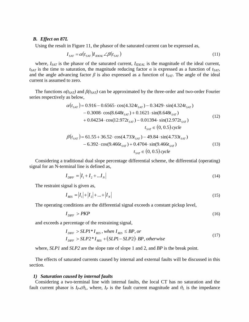
B. Effect on 87L
Using the result in Figure 11, the phasor of the saturated current can be expressed as,
SATIDEALSATSAT tItI (11)
where, ISAT is the phasor of the saturated current, IIDEAL is the magnitude of the ideal current,
tSAT is the time to saturation, the magnitude reducing factor α is expressed as a function of tSAT,
and the angle advancing factor β is also expressed as a function of tSAT. The angle of the ideal
current is assumed to zero.
The functions α(tSAT) and β(tSAT) can be approximated by the three-order and two-order Fourier
series respectively as below,
cyclet
tt
tt
ttt
SAT
SATSAT
SATSAT
SATSATSAT
5.0,0
)12.972sin(01394.0)12.972cos(04234.0
)648.8sin(1621.0)648.8cos(3008.0
)324.4sin(3429.0)324.4cos(6565.0916.0
(12)
cyclet
tt
ttt
SAT
SATSAT
SATSATSAT
5.0,0
)466.9sin(4704.0)466.9cos(392.6
)733.4sin(84.49)733.4cos(52.3655.61
(13)
Considering a traditional dual slope percentage differential scheme, the differential (operating)
signal for an N-terminal line is defined as,
NDIFF IIII ...21 (14)
The restraint signal is given as,
NRES IIII ...21 (15)
The operating conditions are the differential signal exceeds a constant pickup level,
PKPIDIFF (16)
and exceeds a percentage of the restraining signal,
otherwiseBPSLPSLPISLPI
orBPIwhenISLPI
RESDIFF
RESRESDIFF
,21*2
,,*1
(17)
where, SLP1 and SLP2 are the slope rate of slope 1 and 2, and BP is the break point.
The effects of saturated currents caused by internal and external faults will be discussed in this
section.
1) Saturation caused by internal faults
Considering a two-terminal line with internal faults, the local CT has no saturation and the
fault current phasor is IP∠θL, where, IP is the fault current magnitude and θL is the impedance

angle. The remote CT experiences saturation and the current phasor is α(tSAT)KIP∠(β(tSAT)+γ+θL ),
where, γ is an angle difference tolerance factor to accommodate angle error, and K is a magnitude
difference tolerance factor to accommodate,
Different fault current level at the remote end
Different CT performance between CTs located at two terminals
Model difference between simplified saturation and real saturation
Other errors caused by DC offset, asymmetrical saturation, etc.
Since θL has no effect on the differential calculation, it can be ignored, and then the local and
remote current phasors are expressed as,
))(()(
SATPSATR
PL
tKItI
II (18)
The differential current is then given as,
))(()(1
))(()(
SATSATP
SATPSATPRLDIFF
tKtI
tKItIIII (19)
The restraint current is given as,
KtI
KItIIII
SATP
PSATPRLRES
)(1
)(
(20)
In this scenario, IP is normally greater than the break point BP, so the operating signal is
determined by the following condition,
1)21(2
BPSLPSLPISLP
I
RES
DIFF (21)
Because (SLP1-SLP2) is always less than 0, a more strict operating condition is given below,
12
RES
DIFF
ISLP
I (22)
i.e.,
1
12
)()cos(21
12
)(1 2
KSLP
KK
KSLP
K
(23)
Furthermore, the above equation can be expressed as,
2
1
)()cos(211
2
SLPK
KK
(24)
The Dependability Factor (DF) is defined below to demonstrate the dependability of the
differential function during internal faults,
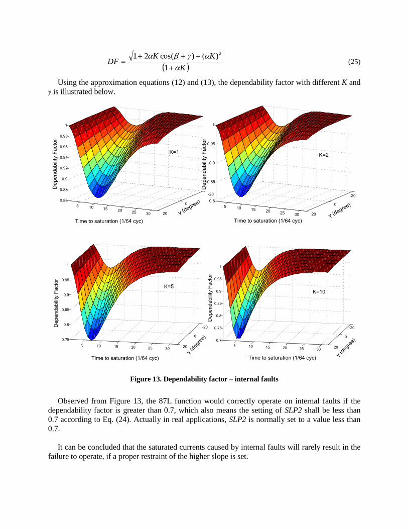
K
KKDF
1
)()cos(21 2
(25)
Using the approximation equations (12) and (13), the dependability factor with different K and
γ is illustrated below.
γ (degree)
γ (degree)
Time to saturation (1/64 cyc) Time to saturation (1/64 cyc)
-20
0
20
5 10 15 20 25 30
0.86
0.88
0.9
0.92
0.94
0.96
0.98
1
De
pe
nd
ab
ility
Fa
cto
r
-20
0
20
5 10 15 20 25 30
0.8
0.85
0.9
0.95
1
De
pe
nd
ab
ility
Fa
cto
r
K=2K=1
γ (d
egre
e)
γ (d
egre
e)
Time to saturation (1/64 cyc) Time to saturation (1/64 cyc)
-20
0
205 10 15 20 25 30
0.75
0.8
0.85
0.9
0.95
1
De
pe
nd
ab
ility
Fa
cto
r
-20
0
205 10 15 20 25 30
0.7
0.75
0.8
0.85
0.9
0.95
1
De
pe
nd
ab
ility
Fa
cto
r
K=10K=5
Figure 13. Dependability factor – internal faults
Observed from Figure 13, the 87L function would correctly operate on internal faults if the
dependability factor is greater than 0.7, which also means the setting of SLP2 shall be less than
0.7 according to Eq. (24). Actually in real applications, SLP2 is normally set to a value less than
0.7.
It can be concluded that the saturated currents caused by internal faults will rarely result in the
failure to operate, if a proper restraint of the higher slope is set.
Even the above analysis and conclusion is based on the simplified saturated waveforms, they
can still be applied for the real applications based on the following factors:
Tolerance factors K and γ already accommodate the magnitude difference, magnitude error, and angle error.
A more strict operating condition, Eq. (22), increases the restraint region and reduces the relay dependability in the analysis; fortunately, the higher slope in the traditional dual slope percentage plane would provide more dependability for the saturation caused by internal faults.
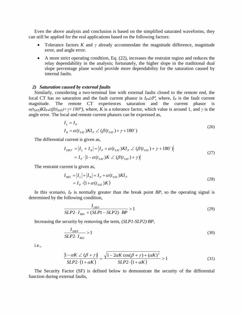
2) Saturation caused by external faults
Similarly, considering a two-terminal line with external faults closed to the remote end, the
local CT has no saturation and the fault current phasor is IP∠0°, where, IP is the fault current
magnitude. The remote CT experiences saturation and the current phasor is
α(tSAT)KIP∠(β(tSAT)+γ+180°), where, K is a tolerance factor, which value is around 1, and γ is the
angle error. The local and remote current phasors can be expressed as,
)180)(()(
SATPSATR
PL
tKItI
II (26)
The differential current is given as,
))(()(1
)180)(()(
SATSATP
SATPSATPRLDIFF
tKtI
tKItIIII
(27)
The restraint current is given as,
KtI
KItIIII
SATP
PSATPRLRES
)(1
)(
(28)
In this scenario, IP is normally greater than the break point BP, so the operating signal is
determined by the following condition,
1)21(2
BPSLPSLPISLP
I
RES
DIFF (29)
Increasing the security by removing the term, (SLP1-SLP2)·BP,
12
RES
DIFF
ISLP
I (30)
i.e.,
1
12
)()cos(21
12
)(1 2
KSLP
KK
KSLP
K
(31)
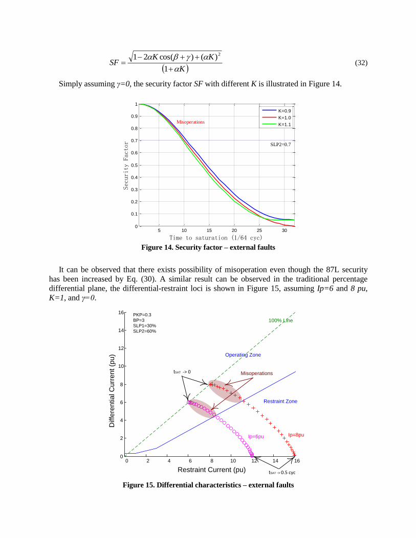
The Security Factor (SF) is defined below to demonstrate the security of the differential
function during external faults,
K
KKSF
1
)()cos(21 2
(32)
Simply assuming γ=0, the security factor SF with different K is illustrated in Figure 14.
Figure 14. Security factor – external faults
It can be observed that there exists possibility of misoperation even though the 87L security
has been increased by Eq. (30). A similar result can be observed in the traditional percentage
differential plane, the differential-restraint loci is shown in Figure 15, assuming Ip=6 and 8 pu,
K=1, and γ=0.
100% Line
Operating Zone
Restraint Zone
Ip=6pu Ip=8pu
tSAT -> 0
0 2 4 6 8 10 12 14 160
2
4
6
8
10
12
14
16
Restraint Current (pu)
Diffe
ren
tia
l C
urr
en
t (p
u)
tSAT -> 0.5 cyc
Misoperations
PKP=0.3
BP=3
SLP1=30%
SLP2=60%
Figure 15. Differential characteristics – external faults
5 10 15 20 25 300
0.1
0.2
0.3
0.4
0.5
0.6
0.7
0.8
0.9
1
Time to saturation (1/64 cyc)
Security Factor
K=0.9
K=1.0
K=1.1Misoperations
SLP2=0.7
It can be concluded that CT saturation caused by external faults, particularly when it is more
severe at one CT carrying the whole fault current in breaker-and-a-half applications or when CTs
are different at opposite line terminals, introduces a spurious differential current that may cause
the differential protection to misoperate.
IV. TECHNIQUES USED TO IMPROVE CT SATURATION TOLORENCE FOR 87L APPLICATIONS
It has been mentioned that it is not always practical to avoid CT saturation in real applications
by using Equations (7) and (9) to size CT. Therefore, some techniques have to be applied in relays
to deal with problems caused by CT saturation.
Based on the analysis in the previous section, protection engineers are mostly concerned with
the techniques to increase the security during saturation caused by external faults.
External fault detectors are commonly applied in bus or transformer protection. These methods
detect external faults before the occurrence of CT saturation to prevent relay misoperation on
external faults.
Saturation detection techniques have been developed as well to block/unblock the operation of
protection elements. These algorithms are slower than the external fault detectors that specially
use sampled-based detection techniques, because saturation detectors would be asserted until the
occurrence of CT saturation.
Some compensation methods have been proposed to reconstruct the distorted secondary
current waveform caused by saturation conditions. Then, the reconstructed and undistorted
waveform will be used for relay calculations. However, there still have some issues for real
implementation, such as precision, speed and computation burden.
With respect to the application of current differential relays, one or more extra security
measures listed below can be applied upon the detection the external fault.
Add a portion of current distortions such as harmonics, saturated CT signal and noise, into the restraint signal; therefore, the restraint region is adaptively increased.
Dynamically switch the differential settings to more secure values to deal with external faults. Normally, the more secure settings would result in the larger restraint region.
Constantly use the transient bias as the additional restraint signal. An external fault or a sudden surge of the load current will cause a positive change (delta) in the restraint current, and then this delta signal is mixed into the transient bias to increase the restraint signal. If the delta signal vanished, the transient bias would start decaying exponentially.
A technique utilizing the adaptive restraint and CT saturation detection is explained below in
details [15], [16].
The adaptive restraint characteristic dynamically adjusts the operating-restraint boundary
which is the decision boundary between situations that are declared to be a fault and those that are
not. The adaptive decision process is based on an on-line computation of the sources of

measurement error. Sources of error include power system noise, transients, inaccuracy in line
charging current computation, current sensor gain, phase and saturation error, clock error, and
asynchronous sampling.
The relay computes the error caused by power system noise, CT saturation, harmonics, and
transients. These errors arise because power system currents are not always exactly sinusoidal.
The intensity of these errors varies with time; for example, growing during fault conditions,
switching operations, or load variations. Current transformer saturation is included with noise and
transient error. The measurement error, also called goodness of fit, is computed as a sum of
squared differences between the actual waveform and an ideal sinusoid over one data window.
2
__
12/
0
2
)(_
2
)(__
44AMAGLOC
NC
p
pkALOCkAADALOC IiNCNC
I (33)
where, ILOC_ADA_A is the local phase A adaptive restraint term, NC is the amount of samples per
cycle, iLOC_A is the local phase A samples after the dc removal filtering, and ILOC_MAG_A is the local
phase A magnitude.
A dedicated mechanism is applied in the line current differential relay to cope with CT
saturation and ensure security of protection for external faults. The relay dynamically increases
the weight of the adaptive restraint portion (ILOC_ADA_A in Eq. (33)) in the total restraint quantity,
but for external faults only. The following logic is applied:
First, the terminal currents are compared against a threshold of 3 pu to detect overcurrent conditions that may be caused by a fault and may lead to CT saturation.
For all the terminal currents that are above the 3 pu level, the relative angle difference is calculated.
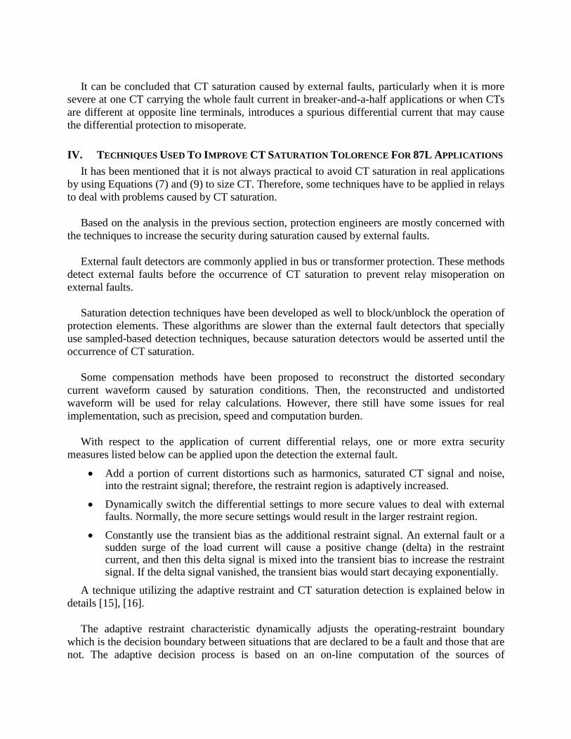
Depending on the angle difference between the terminal currents, the adaptive restraint current is increased by the multiple factor of 1, 5, or 2.5 to 5 as shown in Figure 16. As seen from the figure, a factor of 1 is used for internal faults, and a factor of 2.5 to 5 is used for external faults. This allows the relay to be simultaneously sensitive for internal faults and robust for external faults with a possible CT saturation.
If more than one CT is connected to the relay (breaker-and-the half applications), the CT saturation mechanism is executed between the maximum local current against the sum of all others, then between the maximum local and remote currents to select the secure multiplier MULT. A maximum of two (local and remote) is selected and then applied to adaptive restraint.
arg(ILOC/IREM)=0
(internal fault)
MULT=1
MULT=1
MULT=abs(arg(ILOC/IREM)×5/180
arg(ILOC/IREM)=180(external fault)
MULT=5
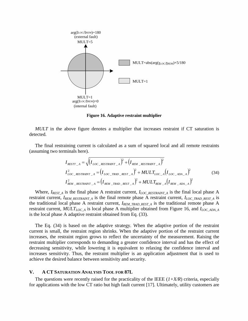
Figure 16. Adaptive restraint multiplier
MULT in the above figure denotes a multiplier that increases restraint if CT saturation is
detected.
The final restraining current is calculated as a sum of squared local and all remote restraints
(assuming two terminals here).
2___
2
___
2
__
2
___
2
___
2
__
2
__
2
___
AADAREMAREMARESTTRADREMARESTRAINTREM
AADALOCALOCARESTTRADLOCARESTRAINTLOC
ARESTRAINTREMARESTRAINTLOCARESTT
IMULTII
IMULTII
III
(34)
Where, IREST_A is the final phase A restraint current, ILOC_RESTRAINT_A is the final local phase A
restraint current, IREM_RESTRAINT_A is the final remote phase A restraint current, ILOC_TRAD_REST_A is
the traditional local phase A restraint current, IREM_TRAD_REST_A is the traditional remote phase A
restraint current, MULTLOC_A is local phase A multiplier obtained from Figure 16, and ILOC_ADA_A
is the local phase A adaptive restraint obtained from Eq. (33).
The Eq. (34) is based on the adaptive strategy. When the adaptive portion of the restraint
current is small, the restraint region shrinks. When the adaptive portion of the restraint current
increases, the restraint region grows to reflect the uncertainty of the measurement. Raising the
restraint multiplier corresponds to demanding a greater confidence interval and has the effect of
decreasing sensitivity, while lowering it is equivalent to relaxing the confidence interval and
increases sensitivity. Thus, the restraint multiplier is an application adjustment that is used to
achieve the desired balance between sensitivity and security.
V. A CT SATURATION ANALYSIS TOOL FOR 87L
The questions were recently raised for the practicality of the IEEE (1+X/R) criteria, especially
for applications with the low CT ratio but high fault current [17]. Ultimately, utility customers are
looking for the relay manufacturer recommendations and warranties for the CT selection at their
system with particular relay models. CT selection recommendations are different from one
manufacturer to another and there cannot be any standard giving specific recommendations. It is
possible to verify relay performance for a given application by modelling CTs with RTDS or any
other simulation tools, but this is not always available to utility customer, is expensive and
requires lot of efforts and time.
It is relay manufacturers’ responsibility to confirm the CT/relay system application since only
the relay manufacturer knows the proprietary design of the protection relay [18]. Besides relay
algorithms, complexity arises from the fault current distribution in breaker-and-a-half
applications, possible different CT ratios or even different CT characteristics in real life
applications.
In order to analyze the line current differential relay reliability during CT saturation caused by
an external fault, investigate the effect of adjusting 87L settings, choose the proper size of CT and
examine possibility of reducing CT requirement, it is possible to develop a type of CT saturation
analysis tool that is able to emulate the CTs and the relay behavior. The following description is
an example of such a tool.
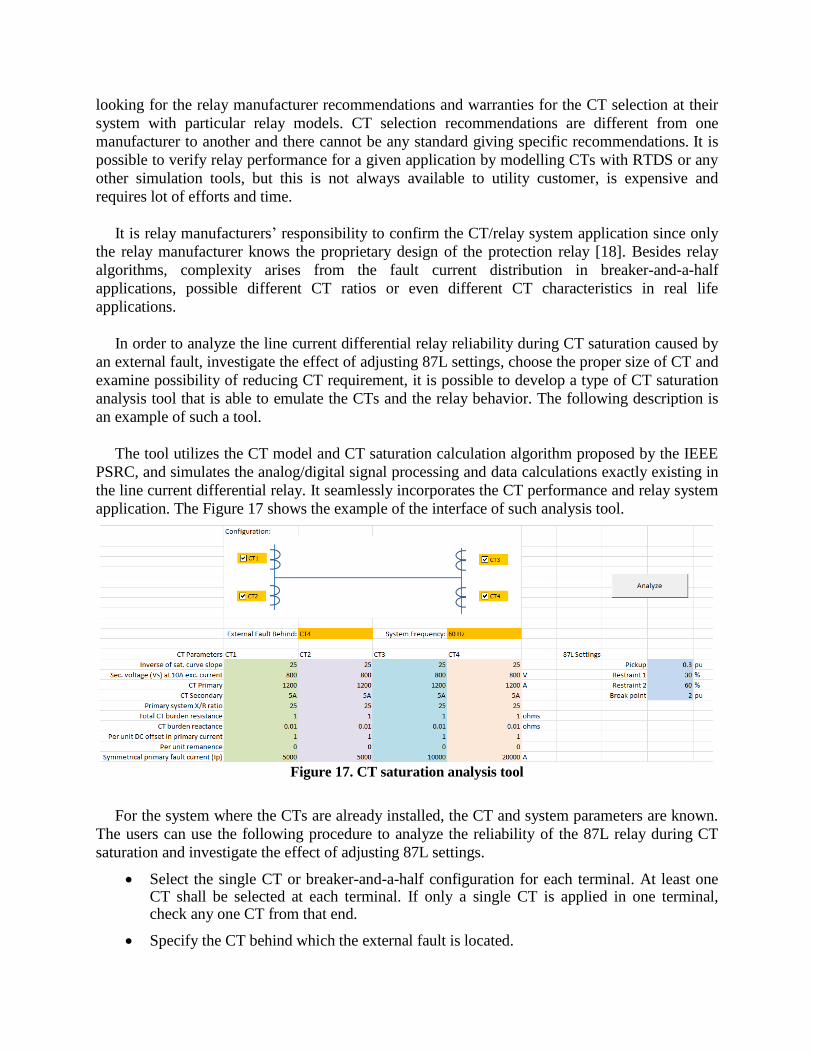
The tool utilizes the CT model and CT saturation calculation algorithm proposed by the IEEE
PSRC, and simulates the analog/digital signal processing and data calculations exactly existing in
the line current differential relay. It seamlessly incorporates the CT performance and relay system
application. The Figure 17 shows the example of the interface of such analysis tool.
Figure 17. CT saturation analysis tool
For the system where the CTs are already installed, the CT and system parameters are known.
The users can use the following procedure to analyze the reliability of the 87L relay during CT
saturation and investigate the effect of adjusting 87L settings.
Select the single CT or breaker-and-a-half configuration for each terminal. At least one CT shall be selected at each terminal. If only a single CT is applied in one terminal, check any one CT from that end.
Specify the CT behind which the external fault is located.

Choose the system frequency, 60Hz or 50Hz.
Based on the datasheet provided by the CT manufacturer, input the CT parameters for each CT, including inverse of saturation curve slope, secondary voltage (Vs) at 10A exciting current, CT primary current, CT secondary current. The details can be referred to the IEEE PSRC documents [10] and [11].
Determine the corresponding primary circuit X/R ratio.
Calculate the total CT burden for each CT, including CT secondary winding resistance, loop lead resistance, and the relay burden at rated secondary current.
Input the per-unit DC offset in primary current, normally set to 1 (100%) for the worst case analysis.
Input the per-unit remanence, normally set to 0 for the selected CTs.
Determine the maximum fault current supplied by each selected CT which is not closed to the external fault. The maximum fault current for the CT closed to the fault is the summation of currents flowing through all other CTs. These currents are in primary amperes.
Set the 87L settings of a percentage differential characteristic, including pickup level, restraint slope 1, restraint slope 2, and break point.
Click the Analyze button, then the CT secondary currents, differential current, restraint current and operate signal will be illustrated. An example is shown in Figure 18.
Try different fault locations and fault distribution through all CTs.
It should be noted that,
Application is considered safe when Irestr/Idiff>1.25 with selected settings and all fault scenarios considered.
Adjusting the 87L settings, especially Restraint 2, is helpful to increase the security during CT saturation caused by external faults.
In the case to size CTs, normally, CT primary and secondary currents can be pre-determined
by some criteria, such as maximum load conditions. The inverse of saturation curve slope is
almost identical for the same CT model, so it can be calculated from the CT datasheet. Therefore,
the users are mostly concerning the selection of VS value. The following procedure can be used.
Set VS to zero and use the approximate CT secondary winding resistance (RCT) for all the CTs to be sized.
The tool will automatically examine the different VS, starting from 3000V to 50V in steps of -50V. Once a misoperation is detected, the tool will stop calculation and give the boundary VS.
Select the CT having the maximum fault current or highest CT primary current, add a 120%~140% safety margin to the boundary VS, find the true VS and secondary winding resistance from the CT datasheet, and input these values into the tool for this CT only.
Repeat the above step until all the CTs are sized.
Try different fault locations and fault distribution through all CTs.

Figure 18. Analysis tool results
VI. TIME TO SATURATION
Because current in an inductance cannot change instantaneously, CTs take time to saturate.
This is an important factor in the design and application of protective relays. For example if a
relay uses digital signal processing to adjust the security of a protective function after CT
saturation has been detected, the relay must have an adequate number of samples prior to
saturation in order to make this determination.
An IEEE report [19] gives the detailed discussion and curves from which the time to saturation
can be estimated. The IEEE standard [1] gives a conservative equation to estimate the time to
saturation.
))((
)(1ln
1
1
BSS
BSSXS
RRIT
RRIVTT
(35)
where, TS is the time to saturation, T1 is the primary system time constant, VX is the saturation
voltage, IS is the primary current divided by the turns ratio, RS is the secondary winding resistance,
and RB is the burden resistance.
A more detailed equation is described in [20], where the dc offset and percent remanence are
included.
cos
1
)()(
)1(1ln
12
121
BSS
xS
RRIoffsetpu
Vremanencepercent
TT
TTTT (36)
where, T2 is the secondary system time constant, and cosφ is the secondary power factor.
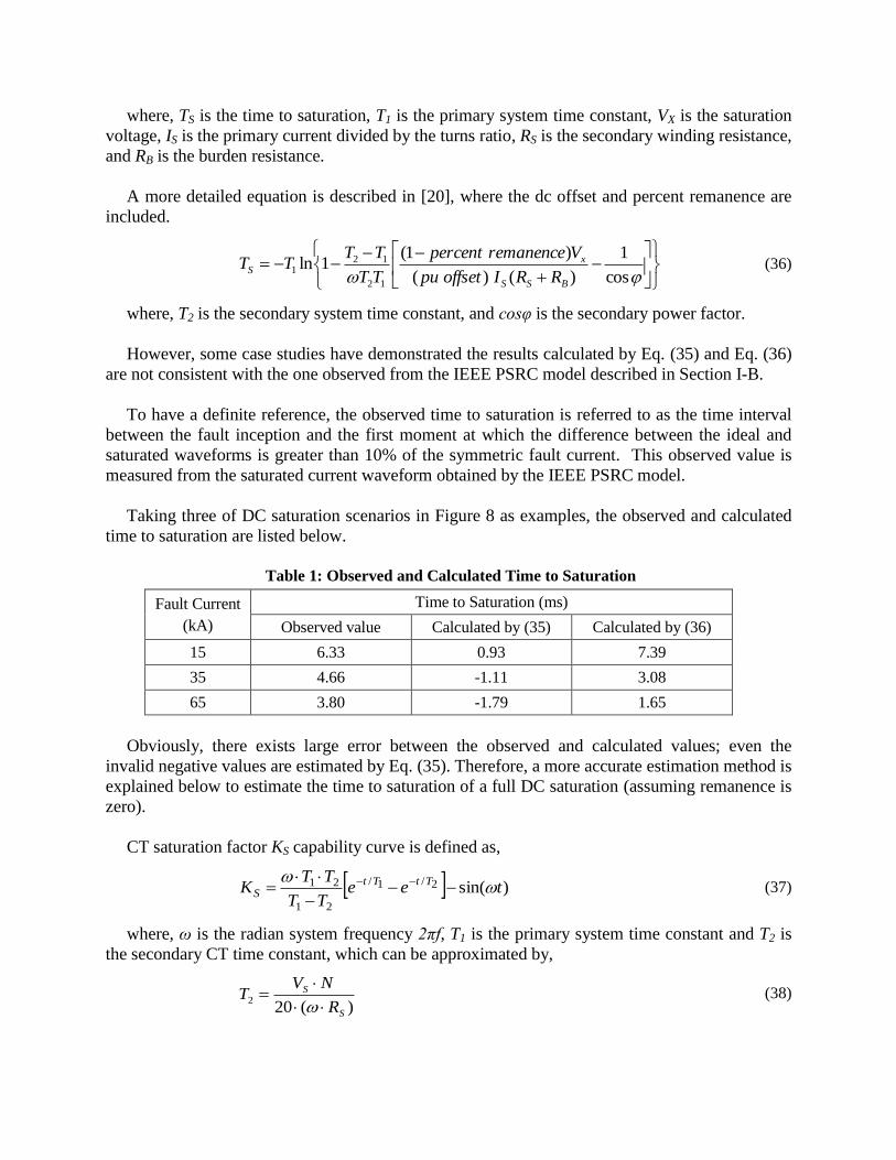
However, some case studies have demonstrated the results calculated by Eq. (35) and Eq. (36)
are not consistent with the one observed from the IEEE PSRC model described in Section I-B.
To have a definite reference, the observed time to saturation is referred to as the time interval
between the fault inception and the first moment at which the difference between the ideal and
saturated waveforms is greater than 10% of the symmetric fault current. This observed value is
measured from the saturated current waveform obtained by the IEEE PSRC model.
Taking three of DC saturation scenarios in Figure 8 as examples, the observed and calculated
time to saturation are listed below.
Table 1: Observed and Calculated Time to Saturation
Fault Current
(kA)
Time to Saturation (ms)
Observed value Calculated by (35) Calculated by (36)
15 6.33 0.93 7.39
35 4.66 -1.11 3.08
65 3.80 -1.79 1.65
Obviously, there exists large error between the observed and calculated values; even the
invalid negative values are estimated by Eq. (35). Therefore, a more accurate estimation method is
explained below to estimate the time to saturation of a full DC saturation (assuming remanence is
zero).
CT saturation factor KS capability curve is defined as,
)sin(2/1/
21
21 teeTT
TTK
TtTtS
(37)
where, ω is the radian system frequency 2πf, T1 is the primary system time constant and T2 is
the secondary CT time constant, which can be approximated by,
)(202
S
S
R
NVT
(38)

where, N is the CT ratio, VS is the CT secondary voltage at 10A exciting current obtained from
CT excitation curve, and RS is the total CT burden.
CT limiting factor KS_LIM is defined by the following equation,
SP
SLIMS
RI
NVK
_
(39)
where, IP is the primary fault current.
Finally, CT time to saturation can be found as a projection of the intersection of the CT
saturation KS capability curve and CT limiting factor KS_LIM as illustrated in the figure below.
Figure 19. Illustration of CT saturation capability curve and limiting factor
Taking the same examples, the time to saturation calculated by the new method is compared
with the observed values, as tabulated below.
Table 2: Observed and Calculated Time to Saturation by New Method
Fault Current
(kA)
Time to Saturation (ms)
Observed value Calculated by new method
15 6.33 6.50
25 5.26 5.33
35 4.66 4.71
45 4.30 4.31
55 4.01 4.02
65 3.80 3.80
It can be observed that the estimation error of the proposed method is normally less than 0.2ms
for the cases studied. The estimation error would become larger when the time to saturation is
longer. The reason is the portion of waveform in the below-knee-point region has been ignored in
the PSRC model; however, this region has a non-negligible effect for slight CT saturation.
Overall, the slight CT saturation (which means longer time to saturation) would have less impact
on the dependability and security of 87L, which can be confirmed from Figure 13 and Figure 14.
It should be mentioned that the well-matched results in Table 2 are obtained from the two
different models. The PSRC model is based on the single-valued saturation curve and the
proposed method is based on the secondary flux curve.
VII. CONCLUSIONS
By analyzing and simulating the simplified saturation current waveforms on the percentage
differential characteristic plane, it has been concluded that,
The saturation caused by internal faults will rarely result in the failure to operate.
The saturation caused by external faults, particularly when it is more severe at one CT carrying the whole fault current in breaker-and-a-half applications or when CTs are different at opposite line terminals, introduces a spurious differential current that may cause the differential protection to misoperate.
The techniques that have been used in 87L to tolerate CT errors, reduce CT requirement and
improve relay security are discussed. An adaptive restraint logic and CT saturation detection
method is explained in details.
Seamlessly incorporating the CT performance and relay system application, a practical CT
saturation analysis tool is presented to analyze reliability of 87L during CT saturation, evaluate
the differential relay security, investigate the effect of adjusting 87L settings, choose the proper
size of CT and examine the possibility of reducing CT requirement. This tool can also be applied
for different applications, including breaker-and-a-half or ring configurations. Furthermore, a
more accurate method is described to estimate the time to saturation.
VIII. REFERENCES
[1] IEEE Guide for the Application of Current Transformers Used for Protective Relaying Purposes,
IEEE Standard C37.110-2007, April 2008.
[2] IEC Instrument transformers – Part 2: Additional requirements for current transformers, IEC
Standard 67869-2, September 2012.
[3] R. Hunt, L. Sevov, and I. Voloh, "Impact of CT Errors on Protective Relays - Case Studies and
Analysis," in Proc. the Georgia Tech Fault & Disturbance Analysis Conference, May 19-20, 2008.
[4] IEEE Standard Requirements for Instrument Transformers, IEEE Standard C57.13-1993, June 1993.
[5] Working Group C-5 of the Systems Protection Subcommittee of the IEEE Power System Relaying
Committee, "Mathematical Models for Current, Voltage, and Coupling Capacitor Voltage
Transformers," IEEE Transactions on power delivery, vol. 15, no. 1, pp. 62-72, January 2000.
[6] Electric Power Research Institute, Electromagnetic Transient Program (EMTP) Rule Book, EPRI
EL-4541, April 1986.
[7] M. Kezunovic, L. Kojovic, A. Abur, C. W. Fromen, D. R. Sevcik, and F. Phillips, "Experimental
Evaluation of EMTP-based Current Transformer Models for Protective Relay Transient Study,"
IEEE Transactions on power delivery, vol. 9, no. 1, pp. 405-413, January 1994.

[8] J. R. Lucas, P. G. McLaren, and R. P. Jayasinghe, "Improved simulation models for current and
voltage transformers in relay studies, " IEEE Trans. on Power Delivery, vol. 7, no. 1, pp. 152-159,
January 1992.
[9] U. D. Annakkage, P. G. McLaren, E. Dirks, R. P. Jayasinghe, and A. D. Parker, "A current
transformer model based on the Jiles-Atherton theory of ferromagnetic hysteresis," IEEE Trans. on
Power Delivery, vol. 15, no. 1, pp. 57-61, January 2000.
[10] Working Group Report of the IEEE Power System Relaying Committee, Theory for CT SAT
Calculator, http://www.pes-psrc.org/Reports/CT_SAT%2010-01-03.zip, 2003.
[11] Working Group Report of the IEEE Power System Relaying Committee, CT SAT Calculator,
http://www.pes-psrc.org/Reports/CT_SAT%2010-01-03.zip, 2003.
[12] B. Kasztenny, J. Mazereeuw, and H. DoCarmo, "CT Saturation in Industrial Applications – Analysis
and Application Guidelines," in Proc. the 60th Annual Conference for Protective Relay Engineers,
March 27-29, 2007.
[13] Working Group Report of the Western Systems Coordinating Council, Relaying Current
Transformer Application Guide, https://www.wecc.biz/Reliability/Relaying%20Current%20
Transformer%20Application%20Guide.pdf, June 1989.
[14] S. Ganesan, "Selection of current transformers and wire sizing in substations," in Proc. the 59th
Annual Conference for Protective Relay Engineers, April 4-6, 2006.
[15] M. G. Adamiak, W. Premerlani, and G. E. Alexander, "A New Approach to Current Differential
Protection for Transmission Lines," in Proc. the Electric Council of New England Protective
Relaying Committee Meeting, October 22-23, 1998.
[16] GE publication GEK-119623, L90 Line Current Differential System - Instruction Manual, 2014.
[17] R. E. Cossé, Jr., D. G. Dunn, and R. M. Spiewak, " CT Saturation Calculations: Are They Applicable
in the Modern World? - Part I: The Question," in Proc. Petroleum and Chemical Industry Technical
Conference, September 12-14, 2005.
[18] R. E. Cossé, Jr., D. G. Dunn, R. M. Spiewak, S. E. Zocholl, T. Hazel, and D. T. Rollay, "CT
Saturation Calculations - Are they Applicable in the Modern World? - Part II, Proposed
Responsibilities," in Proc. Petroleum and Chemical Industry Technical Conference, September 17-
19, 2007.
[19] IEEE PSRC Report, Transient Response of Current Transformers, IEEE Publication 76 CH 1130-4
PWR, January 1976.
[20] A. Wu, "The Analysis of Current Transformer Transient Response and Its Effect on Current Relay
Performance," IEEE Trans. on Industry Applications, vol. IA-21, no. 4, pp. 793-802, May/June 1985.
IX. BIOGRAPHIES
Zhihan Xu received the B.Sc. and M.Sc. degrees in power engineering from Sichuan University, the
second M.Sc. degree in control systems from the University of Alberta, and a Ph.D. degree in power
systems from the University of Western Ontario. He is a Lead Application Engineer with GE Digital
Energy in Markham. His areas of interest include power system protection and control, fault analysis,
modeling, simulation, and automation. He is a professional engineer registered in the province of Ontario.
Matt Proctor is currently a Technical Application Engineer at GE Multilin and has been with GE
Multilin for over 5 years. Matt earned Bachelor of Science in electrical engineering from Louisiana State
University in Baton Rouge, LA in 2001 and an MBA from LSU in 2005. He has been working in the
electrical power field in various capacities since 1997. He specializes in power system studies and
protection and control relay applications. He is a licensed professional engineer in the state of Louisiana
Ilia Voloh received his Electrical Engineering degree from Ivanovo State Power University, Russia. After
graduation he worked for Moldova Power Company for many years in various progressive roles in
Protection and Control field. He is currently an applications engineering manager with GE Multilin in
Markham Ontario, and he has been heavily involved in the development of UR-series of relays. His areas
of interest are current differential relaying, phase comparison, distance relaying and advanced
communications for protective relaying. Ilia authored and co-authored more than 30 papers presented at
major North America Protective Relaying conferences. He is an active member of the PSRC, member of
the main PSRC committee and a senior member of the IEEE.
Mike Lara received his BSEE degree from Texas A&M University in 1990. He spent 4 years with
ExxonMobil and another 6 years with LyondellBasell as a Power Systems Engineer and Project Manager.
He joined SNC-Lavalin in 2000 as a Senior Electrical Design Engineer and has spent the last 15 years in
that capacity specializing in medium and high voltage substations and protective relaying systems for
petrochemical installations. He is a Professional Engineer registered in the state of Texas.


