Computational Science and Engineering(Int. Master’s Program)
Technische Universitat Munchen
Master’s thesis in Computational Science and Engineering
Preconditioning for Hessian-FreeOptimization
Robert Seidl

Computational Science and Engineering(Int. Master’s Program)
Technische Universitat Munchen
Master’s thesis in Computational Science and Engineering
Preconditioning for Hessian-Free Optimization
Author: Robert Seidl1st examiner: Prof. Dr. Thomas Huckle2nd examiner: Prof. Dr. Michael BaderThesis handed in on: April 2, 2012

I hereby declare that this thesis is entirely the result of my own work except whereotherwise indicated. I have only used the resources given in the list of references.
April 2, 2012 Robert Seidl
i
Abstract
Recently Martens adapted the Hessian-free optimization method for the training ofdeep neural networks. One key aspect of this approach is that the Hessian is nevercomputed explicitly, instead the Conjugate Gradient(CG) Algorithm is used to com-pute the new search direction by applying only matrix-vector products of the Hessianwith arbitrary vectors. This can be done efficiently using a variant of the backpropaga-tion algorithm. Recent algorithms use diagonal preconditioners to reduce the needediterations of the CG algorithm. They are used because of their easy calculation andapplication. Unfortunately in later stages of the optimization these diagonal precondi-tioners are not as well suited for the inner iteration as they are for the optimization inthe earlier stages. This is mostly due to an increased number of elements of the denseHessian having the same order of magnitude near an optimum.We construct a sparse approximate inverse preconditioner (SPAI) that is used to accel-erate the inner iteration especially in the later stages of the optimization. The qualityof our preconditioner depends on a predefined sparsity pattern. We apply the knowl-edge of the pattern of the Gauss-Newton approximation of the Hessian to efficientlyconstruct the needed pattern for our preconditioner which can then be computed ef-ficiently fully in parallel using GPUs. This preconditioner is then applied to a deepauto-encoder test case using different update strategies.
ii
Contents
Abstract i
Outline of the Thesis iv
I. Introduction 1
II. Theory 5
1. Iterative Solution of Linear Equation Systems 61.1. Stationary Iterative Methods . . . . . . . . . . . . . . . . . . . . . . . . . . 6
1.1.1. Jacobi Method . . . . . . . . . . . . . . . . . . . . . . . . . . . . . . 71.1.2. Gauss-Seidel Method . . . . . . . . . . . . . . . . . . . . . . . . . . 7
1.2. Nonstationary Iterative Methods . . . . . . . . . . . . . . . . . . . . . . . 71.2.1. Conjugate Gradient Method . . . . . . . . . . . . . . . . . . . . . . 81.2.2. GMRES Method . . . . . . . . . . . . . . . . . . . . . . . . . . . . 9
2. Preconditioning 112.1. Implicit preconditioners . . . . . . . . . . . . . . . . . . . . . . . . . . . . 112.2. Explicit preconditioners . . . . . . . . . . . . . . . . . . . . . . . . . . . . 11
3. Hessian-free Optimization 143.1. Truncated Newton Methods . . . . . . . . . . . . . . . . . . . . . . . . . . 143.2. Levenberg-Marquardt Method . . . . . . . . . . . . . . . . . . . . . . . . 153.3. Implemented algorithm . . . . . . . . . . . . . . . . . . . . . . . . . . . . 163.4. Hessian vs Gauss-Newton approximation . . . . . . . . . . . . . . . . . . 163.5. Inner iteration of the HF method . . . . . . . . . . . . . . . . . . . . . . . 173.6. Preconditioning of inner iteration . . . . . . . . . . . . . . . . . . . . . . . 193.7. Peculiarities of Martens implementation . . . . . . . . . . . . . . . . . . . 20
4. Neural networks 214.1. Feed-forward Networks . . . . . . . . . . . . . . . . . . . . . . . . . . . . 214.2. Deep auto-encoder . . . . . . . . . . . . . . . . . . . . . . . . . . . . . . . 234.3. Network Training . . . . . . . . . . . . . . . . . . . . . . . . . . . . . . . . 244.4. Error backpropagation . . . . . . . . . . . . . . . . . . . . . . . . . . . . . 254.5. Fast multiplication by the Hessian . . . . . . . . . . . . . . . . . . . . . . 27
Contents iii
4.6. Hessian and Gauss-Newton Hessian for neural networks . . . . . . . . . 29
III. Construction of the SPAI Preconditioner 31
5. Efficient pattern finding 335.1. Gauss-Newton approximation . . . . . . . . . . . . . . . . . . . . . . . . 345.2. Building the sparsity pattern . . . . . . . . . . . . . . . . . . . . . . . . . . 345.3. Summary of the pattern finding method . . . . . . . . . . . . . . . . . . . 35
IV. Case study 37
6. Training of a deep auto-encoder 386.1. Overview . . . . . . . . . . . . . . . . . . . . . . . . . . . . . . . . . . . . . 386.2. Pathological Curvature . . . . . . . . . . . . . . . . . . . . . . . . . . . . . 396.3. Analysis . . . . . . . . . . . . . . . . . . . . . . . . . . . . . . . . . . . . . 406.4. Results for different sparsity pattern . . . . . . . . . . . . . . . . . . . . . 446.5. Results for reduced models . . . . . . . . . . . . . . . . . . . . . . . . . . 466.6. Results using CG for the inner iteration . . . . . . . . . . . . . . . . . . . 48
V. Conclusions and Future Work 51
7. Conclusions 52
8. Future Work 538.1. Parallelization of the method . . . . . . . . . . . . . . . . . . . . . . . . . 538.2. Termination of CG . . . . . . . . . . . . . . . . . . . . . . . . . . . . . . . 538.3. Application of a better approximation of the diagonal of the Hessian . . 538.4. Using more information for the preconditioner . . . . . . . . . . . . . . . 548.5. Efficient calculation of particular entries of the Hessian . . . . . . . . . . 54
Appendix 57
A. Pattern finding idea 57
B. Sparsity Patterns 58
C. Results for different Hessians 60
D. CG results 62
Bibliography 63
Outline of the Thesis
Part I: Introduction
This chapter presents an overview of the thesis and its purpose.
Part II: Theory
CHAPTER 1: ITERATIVE SOLUTION OF LINEAR EQUATION SYSTEMS
This chapter presents the basic theory for the iterative solution of linear equation sys-tems. The first part deals with stationary methods like the Jacobi and Gauss-Seidelmethod. The second part deals with Krylov subspace methods which are nonstation-ary methods that form the basis for the inner iteration of truncated Newton methods.Examples are the Conjugate Gradient method and GMRES.
CHAPTER 2: PRECONDITIONING
How fast iterative methods like CG find a solution depends on spectral properties ofthe underlying matrix. It is often convenient to transform the equation system into asystem that has the same solution but has more favorable spectral properties. This isachieved by finding a suitable preconditioner. We will focus on a sparse preconditionerthat is an approximation of the inverse of A. The main task is to find an appropriatesparsity pattern of A−1 without explicit knowledge.
CHAPTER 3: HESSIAN-FREE OPTIMIZATION
This chapter summarizes the Hessian-Free or Truncated Newton method used for theoptimization of nonlinear functions. It presents basic ideas and discusses peculiaritiesin Martens implementation used for training of deep neural networks. A particular fo-cus lies on the stopping criteria of the inner iteration of the optimization method.
CHAPTER 4: NEURAL NETWORKS
This chapter presents the basics of neural networks that are needed to understand thetheory behind the case study. It deals with training of neural networks, the backprop-agation algorithm used to compute gradient information needed for training of the netand a variant known as the “Pearlmutter trick” used to efficiently compute the matrixvector product of the Hessian Hv with an arbitrary vector.
Outline of the Thesis v
Part III: Construction of the SPAI Preconditioner
This part describes the straightforward approach of Benzi to compute a feasible a priorisparsity pattern for a sparse approximate inverse preconditioner.
CHAPTER 5: PATTERN FINDING
Because of the sparsification costs of the above method it is not economic to applythis method to find a suitable pattern for our preconditioner. This chapter presents anapproach to come up with a suitable pattern by exploiting the known pattern of theGauss-Newton Hessian that is usually used as a substitute of the Hessian in the contextof the Hessian-Free optimization method.
Part IV: Case study
CHAPTER 6: TRAINING OF A DEEP AUTO-ENCODER
In this case study Martens Matlab implementation of the Hessian-Free optimizationmethod is used to train a deep auto-encoder. This task is known to be hard for algo-rithms based only on gradient information like the backpropagation algorithm, espe-cially without pretraining.Then the changing structure of the Gauss-Newton Hessian in the different stages of theoptimization is investigated and results of applying different preconditioners on repre-sentatives of the different stages are presented.Furthermore the final results of the application of the SPAI preconditioner, using differ-ent update strategies in HF using GMRES or CG for the inner iteration with differentstopping criteria based on the value of the quadratic approximation, are discussed .
Part V: Conclusions and Future Work
CHAPTER 7: CONCLUSIONS
This chapter summarizes the thesis.
CHAPTER 8: FUTURE WORK
This chapter presents some possible topics for future work like studies dealing withspeedup of the computation of SPAI preconditioners on a graphics card or a possiblymore efficient way to compute the needed entries of the Hessian for the computationof our preconditioner.

1
Part I.
Introduction
2
Introduction
Recently there are a lot of algorithms trying to incorporate second order informationinto the training of deep neural networks. The task of training these networks is knownto be very hard using common training algorithms like backpropagation.This is mostly due to two reasons. The first one is the well known vanishing gradi-ents problem and the second one is pathological curvature. The latter is making it verytough for algorithms based only on gradient information.It often appears that they get stuck in a local minimum because of pathological curva-ture.Following this reasoning, Martens (2010) [25] successfully applied a variant of the Hessian-free optimization algorithm to the task of learning for deep auto-encoders and morerecently also to recurrent neural networks [26].The Hessian-free optimization method, better known as truncated-newton method,uses the idea of Newton’s method and some globalisation ideas to find the minimumof a nonlinear function. Other than Newton’s method it settles for solving the Newtonequations only approximately using some iterative Krylov subspace method like theConjugate Gradient method. Thus the explicit knowledge of the Hessian is not needed.Instead there is only the need to efficiently compute matrix-vector products of the Hes-sian with arbitrary vectors . This is possible through the well-known Pearlmuttertrick[30], which uses a variant of the backpropagation algorithm for feed forward neuralnetworks.There is also an approach called Krylov subspace decent [34] that explicitly computesa basis of the Krylov subspace for a fixed k < N and numerically optimizes the pa-rameter change within this subspace, using BFGS to minimize the original nonlinearobjective function.
Martens uses a handmade diagonal preconditioner to speed up the inner CG iterationbased on some approximate values of the diagonal entries of the Hessian.A further improvement of the HF method of Martens is the use of a better diagonalpreconditioner using the exact values of the diagonal of the Hessian as supposed in [9].All these methods have in common that they use an easy to compute diagonal precon-ditioner for the inner iteration.We will abandon the restriction of diagonal preconditioning and apply a sparse ap-proximate inverse (SPAI) preconditioner [19],[21] to the Krylov subspace method. Thisapproach has the advantages that the computation can be done completely in paralleland that the preconditioned residuals in the CG algorithm can be obtained by a simplematrix vector product instead of being the solution of a linear equation system.
Introduction 3
As we will see, the choice of diagonal preconditioners makes perfect sense in the earlystages of the optimization, in particular if a Levenberg-Marquardt heuristic, as in Martensmethod, is used to guarantee global convergence of the HF method.The shifted equation system in outer iteration k is given by (Hk + λkI)pk = −gk.In the early stages of the optimization, λ will be greater than zero and the diagonal en-tries will be the dominating entries, therefore it should be sufficient for a preconditionerto capture these entries.
But in later stages, in particular near a minimum, λ will be almost zero and there willbe a lot of elements in H that have the same order of magnitude.Benzi successfully applied a SPAI preconditioner to speed up Krylov subspace meth-ods even if the considered matrices are dense [5]. This is also the case for our Hessian.
It is vital for the success of the preconditioner to capture the positions of the largestelements of A because they tend to also be positions of the largest elements of A−1.We first follow Benzi’s approach to find an optimal pattern for our preconditioner forsome Hessians obtained in the process of optimization. Then we compare the perfor-mance of our SPAI preconditioner for different drop tolerances, and therefore differentsparsity patterns, and show their superiority to the performance of other common pre-conditioners like ILU, Jacobi or Gauss-Seidel, even though most of them are clearlyunpractical for the HF method.Then we discuss how we can use cheaply available information in the HF method tocome up with a good guess for the needed sparsity pattern of our preconditioner usingknowledge how the Gauss-Newton approximation of the Hessian is built and comparethe performance of our preconditioner for a fixed sparsity.
With this simple and efficient method to find a good sparsity pattern for our precondi-tioner for a predefined sparsity percentage or number of allowed nonzero elements athand, the preconditioner is incorporated in Martens HF implementation.For simplicity it is first used together with the GMRES method to test different updatestrategies.Because of the comparable high costs to compute the preconditioner , especially if it isnot possible to distribute the computation on a graphics card, it seems economical touse the same SPAI preconditioner for consecutive iterations.We use Martens HF implementation and his standard testcase, the training of the CURVESdataset of a deep auto-encoder, to compare the different update strategies with the un-preconditioned and the diagonally preconditioned variant.
After the successful tests using GMRES instead of CG, we have a closer look at dif-ferent stopping criteria for CG in the context of truncated-newton methods.To only monitor the residual r = b − Ax in the CG method is in general a bad idea ifsomeone wants to stop the iteration before the iterative method actually finds the de-sired solution.This is because CG minimizes a quadratic approximation instead of solving the equa-

Introduction 4
tion system directly. Thus the value of the quadratic function is monotonically decreas-ing but not the residual.Therefore it is better to use a stopping criteria that monitors the value of the quadraticapproximation. Martens uses a handmade criteria to stop the inner iteration in [25].

5
Part II.
Theory
6
1. Iterative Solution of Linear EquationSystems
In many applications linear equation systems are obtained after discretization of a prob-lem. Thus it is often enough to compute only an approximate solution in the alreadyintroduced order of the discretization error. An approximate solution is usually com-puted way faster than the exact solution.An iterative method finds an infinite sequence of approximate solutions to the exactsolution of the linear system. In the iteration process the error is usually decreased byusing A repeatedly and without modifying.The idea is to produce such a sequence by applying an iterative function Φ.
xk+1 = Φ(xk) ⇒ xkk→∞−−−→ x = A−1b. (1.1)
First we introduce Jacobi and Gauss-Seidel methods as examples of stationary iterativemethods.Then we investigate the Conjugate Gradient method and GMRES as examples of non-stationary iterative methods. We follow [1].
1.1. Stationary Iterative Methods
These methods can be written in two normal forms.
• xk+1 = xk + Frk with preconditioner F and residual rk = b−Axk, or
• xk+1 = c+Bxk, where B = I − FA.
The first form formulates the iterative method as a residual based correction scheme.The second one states that xk+1 is obtained by a linear transformation of the previousiterate.Starting from the initial value x0 = 0, the solution at iteration k will lie in the Krylovs-pace Kk(B, c).
xk+1 ∈ Kk(B, c) := span¦c,Bc,B2c, . . . , Bk−1c
©(1.2)
Stationary methods differ in the choice of the iteration matrix B resp. preconditionerF .
1. Iterative Solution of Linear Equation Systems 7
1.1.1. Jacobi Method
To obtain the Jacobi method, we first write the equation system row-wise.nXj=1
aijxj = bi
Then we solve the equation in row i for xi while assuming that the other entries of xremain fixed.
xi =1aii
�bi −
Xj 6=i
aijxj
�This suggests an iterative method
x(k+1)i =
1aii
�bi −
Xj 6=i
aijx(k)j
�In matrix terms, the Jacobi method can be expressed as
x(k+1) = D−1(L+ U)x(k) +D−1b
where the matrices D,−L,−U represent the diagonal, the strictly lower-triangular, andthe strictly upper-triangular parts of A.
1.1.2. Gauss-Seidel Method
If we proceed as with the Jacobi method, but now assume that the equations are exam-ined one at a time in sequence, and that previously computed results are used as soonas they are available, we obtain the Gauss-Seidel method:
x(k+1)i =
1aii
�bi −
Xj<i
aijx(k+1)j −
Xj>i
aijx(k)j
�
x(k+1) = (D − L)−1(Ux(k) + b) = x(k) + (D − L)−1rk
where the matrices D,−L,−U represent the diagonal, the strictly lower-triangular, andthe strictly upper-triangular parts of A.
The convergence of these methods depends on the spectral radius of the iteration ma-trix B, i.e. ρ(B) < 1. This is for example true for strictly diagonal dominant matrices.
1.2. Nonstationary Iterative Methods
Nonstationary methods differ from stationary methods in that the computations in-volve information that changes at each iteration. Typically, constants are computed bytaking inner products of residuals or other vectors arising from the iterative method.
1. Iterative Solution of Linear Equation Systems 8
1.2.1. Conjugate Gradient Method
The Conjugate Gradient method is an effective method for symmetric positive definitesystems, thus it is the perfect candidate to approximately solve the Newton equation ina truncated Newton method.Instead of solving Ax = b, CG minimizes the quadratic Φ(x)
Φ(x) =12xTAx− xT b.
The approximate solutions are updated by the formula
x(k) = x(k−1) + αkp(k), (1.3)
where αk is the stepsize and p(k) the search direction.The stepsize αk is found by a one-dimensional minimization of Φ(x(k) + αkp
(k)) as
αk =r(k−1)T r(k−1)
p(k)TAp(k), (1.4)
where the residual r(k) = b−Ax(k) is updated as
r(k) = r(k−1) − αkq(k), (1.5)
where q(k+1) = Ap(k+1).Then the search direction is updated using the residuals
p(k) = r(k) + βk−1p(k−1), (1.6)
where the choice βk = r(k)T r(k)
r(k−1)T r(k−1)ensures that p(k) and Ap(k−1) are orthogonal.
In fact, the choice of βk ensures that p(k) and r(k) are orthogonal to all previous Ap(j)
and r(j) respectively.Since for symmetricA an orthogonal basis for the Krylov subspace span{r(0), . . . , Ai−1r(0)}
can be constructed with only three-term recurrences, such a recurrence also suffices forgenerating the residuals. In the Conjugate Gradient method two coupled two-term re-currences are used, one that updates residuals using a search direction vector. and oneupdating the search direction with a newly computed residual. This makes the Conju-gate Gradient Method computationally attractive.Listing 1.1 shows an implementation of the preconditioned algorithm.Note that to get fast convergence and reduce the number of iterations, it is often neededto apply a suitable preconditioner M , such that M−1Ax = M−1b has more favorablespectral properties, i.e. clustered eigenvalues.The preconditioned CG method using preconditioner M = LLT minimizes the follow-ing quadratic form.
ϕ2(y) =12yTLTALy − yTLT b,
1. Iterative Solution of Linear Equation Systems 9
r(0) = b−Ax(0)for initial guess x(0)
for k = 1 , 2 , . . .so lve Mz(k−1) = r(k−1)
p(k−1) = r(k−1)T z(k−1);i f k == 1
p(1) = z(0);e lse
βk−1 = p(k−1)/p(k−2);p(k) = z(k−1) + βk−1p
(k−1);endq(k) = Ap(k);αk = p(k−1)
p(k)T q(k) ;x(k) = x(k−1) + αkp
(k);r(k) = r(k−1) − αkq(k)
i f r(k) < ε
return ;end
end
Listing 1.1: The Conjugate Gradient method
where y = L−1x.After n steps of the CG method Kn(A, b) = Rn and therefore xn = A−1b is the solutionin exact arithmetic. This is not true in floating point arithmetic.For CG, the error can be bounded in terms of the spectral condition number of thematrix M−1A. If x is the exact solution of the linear system Ax = b, with symmetricpositive definite matrix A, then for CG, it can be shown that x(k) − x
A≤ 2γk
x(0) − x A
where γ =√κ−1√κ+1
and κ = κ(M−1A) = λmaxλmin
.Note that CG tends to eliminate components of the error in the direction of eigenvec-tors associated with extremal eigenvalues first. After these have been eliminated, themethod proceeds as if these eigenvalues did not exist in the given system, i.e. the con-vergence rate depends on a reduced system with a smaller condition number. See [33]for an analysis of this.It is possible to compute a preconditioner for the CG method that makes use of this.See Section 8.4 for more information.
1.2.2. GMRES Method
In the Conjugate Gradients method, the residuals form an orthogonal basis for the spacespan{r(0), Ar(0), A2r(0), . . .}.
1. Iterative Solution of Linear Equation Systems 10
In GMRES, this basis is formed explicitly.
w(i) = Av(i)
for k = 1 , . . . , iw(i) = w(i) − (w(i), v(k))v(k)
endv(i+1) = w(i)
‖w(i)‖Listing 1.2: Orthogonal basis of the Krylov space
This is a modified Gram-Schmidt orthogonalization. Applied to the Krylow sequence{Akr(0)} this orthogonalization is called the Arnoldi method. The inner product coeffi-cients (w(i), v(k)) and
w(i) are stored in an upper Hessenberg matrix.
The GMRES iterates are constructed as
x(i) = x(0) + y1v(1) + · · ·+ yiv
(i),
where the coefficients yk have been chosen to minimize the residual norm b−Ax(i)
.Note that, while the CG method is both, cheap and optimal, GMRES is only an optimalmethod. With increasing iterations the computation and storage of the orthogonal basisof the Krylovspace gets very expensive. Therefore one often settles with a restartedvariant of GMRES.
11
2. Preconditioning
The convergence rate of iterative methods depends on spectral properties of the coef-ficient matrix. Hence one may attempt to transform the linear system into one that isequivalent in the sense that it has the same solution, but has more favorable spectralproperties. A preconditioner is a matrix that effects such a transformation.For instance, if a matrix M approximates the coefficient matrix A in some way, thetransformed system
M−1Ax = M−1b
has the same solution as the original system Ax = b, but the spectral properties of itscoefficient matrix M−1A may be more favorable.In devising a preconditioner, we are faced with a choice between finding a matrix Mthat approximates A, and for which solving a system is easier than solving one withA, or finding a matrix M that approximates A−1, so that only multiplication by M isneeded.The majority of preconditioners falls in the first category, but the preconditioner we willuse will be an approximation of A−1.
2.1. Implicit preconditioners
These preconditioners try to approximate A. Theoretically the perfect preconditioneris M = A−1, or thinking about the LU decomposition of A, we want to choose M =(LU)−1. Of course it is too expensive to actually compute the inverse and then use it aspreconditioner.Nevertheless we can use an approximation of the LU decomposition as implicit pre-conditioner of A.The idea is to let L,U take nonzero values only at nonzero positions of A, i.e. keep thesparsity pattern of A and L + U the same. This is the so-called ILU(0), with no fill-insallowed. The algorithm is shown in listing 2.1.
2.2. Explicit preconditioners
These types of preconditioners try to approximate A−1. Implicit preconditioners arerobust and lead to fast convergence of the preconditioned iteration but are difficult toimplement in parallel. In particular the triangular solves involved in ILU precondition-ing represent a serious bottleneck, thus limiting the performance on parallel computers.
2. Preconditioning 12
for j = 1, . . . , nfor i = j + 1, . . . , n
i f Aij 6= 0Aij = Aij/Ajj ;for k = j + 1, . . . , n
i f Aik 6= 0Aik = Aik −AijAjk ;end ;
end ;end ;
end ;end
Listing 2.1: ILU(0) method
The explicit approach has some advantages over the implicit approach. First the pre-conditioner can be computed fully in parallel and second if used as preconditioner ofthe PCG method there is no equation system My = r to be solved to get the precon-ditioned residual. Instead only one matrix-vector multiplication y = M · r is needed.These computations are easier to parallelize than the triangular solves needed for im-plicit preconditioning. This is why inverse preconditioners are becoming increasinglypopular.We will only consider one special type of preconditioner, the sparse approximate in-verse preconditioner(SPAI). For more information, see [19], [21].
Sparse Approximate Inverse(SPAI) Preconditioner
We can think of a SPAI preconditioner as the best matrix that has a prescribed sparsitypattern S and minimizes the following functional (in the Frobenius norm).
minM‖AM − I‖2F (2.1)
The Frobenius norm naturally decouples (2.1) into n Least Squares problems
minmj‖Amj − ej‖22 , j = 1, . . . , n (2.2)
where M = [m1 . . .mn], I = [e1 . . . en].Thus the computation is embarrassingly parallel.Due to the sparsity of A, equation (2.2) represents an usually small-sized Least-squaresproblem to solve, although n can be very large. Even if A is sparse, A−1 will usuallynot be sparse. The main issue is the selection of the nonzero pattern of M . There aredifferent possibilities we can choose from to create our a priori sparsity pattern.
2. Preconditioning 13
Different choices for the sparsity pattern of M ≈ A−1
We could use the pattern of
• Ak or (AT )k
• (ATA)kAT for some k = 1, 2
• Aε with sparsified A
where Aε is obtained by deleting all entries with |Ai,j | ≤ ε.Following Benzi, [5] an easy way to compute a sparsity pattern of M is the use of asimple criterion based on a threshold parameter ε ∈ (0, 1) and to include position (i, j)in the nonzero pattern of M if
|aij | > max1≤k,l≤n
|akl|. (2.3)
For our deep auto encoder test case, we will compute A explicitly and then sparsifyA using different drop tolerances εi at different iterates to get some insight into thechanging structure of the Gauss-Newton approximation of the Hessian used in the HFalgorithm.This procedure is very expensive and clearly unpractical to use for the pattern findingpart in the HF algorithm.Fortunately we can use cheaply available information about the different magnitudesof the diagonal elements of the Gauss-Newton approximation to find a good sparsitypattern for our preconditioner without explicit knowledge of A.Moreover we are able to find the best pattern for a predefined sparsity percentage of A.We will focus on this in Chapter III.In the context of the Hessian-Free optimization algorithm, the Gauss-Newton Hessianis used instead of the Hessian. This approximation is always symmetric positive defi-nite, therefore it is reasonable to compute our SPAI preconditioner in a factorized formM = LLT . Hence FSPAI, a factorized version of the preconditioner, is used in the tests.See Huckle [20] for more information.
14
3. Hessian-free Optimization
The Hessian-Free optimization method, also known as truncated Newton method, triesto minimize a nonlinear function f . But instead of computing the exact Newton direc-tion −H−1g where H is the Hessian and g the gradient, a truncated Newton methodsolves the system Hd = −g only approximately using e.g. the conjugate gradientmethod. CG is solving the system using only matrix-vector multiplications Hv. Thesemultiplications can be done efficiently using a technique known as the “Pearlmutter-trick”.The Hessian is never computed explicitly and is only available implicitly through matrix-vector products. Thus the name “Hessian-Free”.Martens adapted the Hessian-Free method for the training of deep auto-encoders.This chapter presents the idea of the Hessian-Free optimization method in some detail.Then the subtleties in Martens implementation are discussed. Furthermore we comparethe differences of the Hessian and the Gauss-Newton Hessian and why it is preferableto use the latter one. In the end, we look at different stopping criteria for the inneriteration.
3.1. Truncated Newton Methods
The Hessian-free optimization method is a second order quasi-newton method that op-timizes a given nonlinear function f(w). It doesn’t use a low rank approximation of theHessian. Only the matrix-vector product of the Hessian with a vector d is needed for theoptimization, thus the Hessian is never computed explicitly. Fortunately there exists anefficient algorithm for neural networks that computes these matrix-vector products ex-actly and efficiently in O(w), where w are the weights of the neural network that has tobe trained.
Truncated-Newton methods are a family of methods suitable for solving large non-linear optimization problems. At each iteration, the current estimate of the solution isupdated (i.e., a step is computed) by approximately solving the Newton equations us-ing an iterative algorithm. This results in a doubly iterative method: an outer iterationfor the nonlinear optimization problem, and an inner iteration for the Newton equa-tions. The inner iteration is typically stopped or “truncated” before the solution to theNewton equations is obtained. More generally, an “inexact” Newton method computesa step by approximately solving the Newton equations.We focus on the unconstrained problem
minw
E(w) (3.1)

3. Hessian-free Optimization 15
where the nonlinear function E(w) is for example the sum-of-squares reconstructionerror of our deep auto-encoder.The first-order optimality condition for this problem is
∇E(w) = 0 (3.2)
which is a system of nonlinear equations.Given some guess wk of a solution w, Newton’s method computes a step pk as thesolution to the linear system.
∇2E(wk)pk = −∇E(wk) (3.3)
and then sets wk+1 = wk + pk. In this simple form, Newton’s method is not guaranteedto converge.In a truncated-Newton method, an iterative method is applied to (3.3), and an approx-imate solution accepted.The rate of convergence of the outer iteration is related to the accuracy with which (3.3)is solved.
A basic question in a truncated-Newton method is the choice of an inner iterative algo-rithm for solving (3.3). Some variant of the linear conjugate-gradient method is almostalways used. The conjugate-gradient method is an optimal iterative method for solv-ing a positive-definite linear system Ap = b, in the sense that the kth iterate pk mini-mizes the associated quadratic functionQ(p) = 1
2pTAp− pT b over the Krylov subspace
spanned by {b, Ab, . . . , Ak−1b}.The Hessian matrix∇2E(wk) need not be positive definite, so the assumptions underly-ing the conjugate-gradient method may not be satisfied. However, the Hessian matrixis always symmetric. At a local minimizer of (3.2), the Hessian is guaranteed to bepositive semi-definite. Thus, as the solution is approached, and the Newton model for(3.2) is more accurate and appropriate, we can anticipate that the requirements for theconjugate-gradient method will be satisfied.A truncated-Newton method will only be competitive if further enhancements are used.For example, a preconditioner for the linear system will be needed, and the stoppingrule for the inner algorithm will have to be chosen in a manner that is effective bothclose to and far from the solution. With these enhancements, truncated-Newton meth-ods are a powerful tool for large-scale optimization.
3.2. Levenberg-Marquardt Method
The Levenberg-Marquardt method is a compromise between the following two meth-ods:
• Newton’s method, which converges rapidly near a local or global minimum, butmay also diverge

3. Hessian-free Optimization 16
• Gradient descend, which is assured to converge through a proper selection of thestep-size parameter, but converges slowly.
Consider the modified Newton equations for outer iteration k.
(∇2E(wk) + λI)pk = −∇E(wk) (3.4)
where I is the identity matrix of the same dimensions as H = ∇2E(wk) and λ is a regu-larizing parameter that forces the sum matrix (H+λI) to be positive definite and savelywell conditioned throughout the computation.When λ is large, λI dominates H, the method reduces to the gradient descend method.If λ is small the estimated increment is almost the same as that of the Gauss-Newtonmethod. The value of λ varies at each iteration, depending on whether the objectivefunction decreases.
Martens uses a simple heuristic for adjusting λ.If ρ < 1
4 : λ← 32λ, if ρ > 3
4 : λ← 23λ, where ρ is the “reduction ratio”.
The reduction ratio is a scalar quantity which attempts to measure the accuracy of thequadratic model Q and is given by:
ρ =E(w + p)− E(w)Q(p)−Q(0)
. (3.5)
3.3. Implemented algorithm
for n = 1 , 2 , . . . dogn ← ∇f(wn) compute/adjust λ by some methoddefine the function Bn(d) = H(wn)d+ λdpn ← CG-Minimize(Bn,−gn)wn+1 ← wn + pn
end for
Listing 3.1: The Hessian-Free Optimization Algorithm
3.4. Hessian vs Gauss-Newton approximation
The training error of a neural network is in general a non-convex function, thereforethe Hessian H might not be positive definite, so Newtons method may diverge. Thusmost algorithms use approximations of the Hessian that remain positive definite. Onechoice is the use of the Gauss-Newton approximation of the Hessian. Sometimes it iscalled linearized, outer product or squared Jacobian approximation.
3. Hessian-free Optimization 17
The idea is to approximate the objective function E around wk by a quadratic function.Specifically the Newton algorithm uses the second-order Taylor expansion
W (wk + p) ≈W (wk) + pT∇W (wk) +12pTH(wk)p := Qk(p) (3.6)
The second order taylor expansion is called the Newton approximation of the functionE, as it is related to the Newton algorithm.Similarly when H is replaced by the Gauss-Newton matrix HGN , the quadratic approx-imation is called Gauss-Newton approximation.The Gauss-Newton Hessian is introduced for neural networks in Section 4.6.
3.5. Inner iteration of the HF method
The inner iteration of a truncated Newton method almost always consists of a variantof the Conjugate Gradient algorithm. Additionally to the common residual based stop-ping criterion, there is also a stopping criterion used that depends on the optimizationprogress of the quadratic model.
Algorithm: Truncated Newton (Inner Loop of Outer Step k)
0. Initialization.Set p0 = 0, q0 = qk(p0) = 0, r0 = −g, and d0 = Mr0.
For i = 0, 1, 2, . . . proceed as follows:
1. Negative Curvature TestIf dTi Hdi < 0,exit inner loop
2. Truncation Test.
αi =rTi (Mri)dTi Hdi
pi+1 = pi + αidi
ri+1 = ri − αiHdi
qi+1 =12
(ri+1 + g)T pi+1 Value of Q(pi+1)
If STOPResidual is satisfied for ri+1, or STOPQuadratic is satisfied for Q(pi+1),exit inner loop with search direction p = pi+1.
3. Hessian-free Optimization 18
3. Continuation of PCG
βi =rTi+1(Mri+1)rTi (Mri)
di+1 = (Mri+1) + βidi
Stopping Criteria for inner iteration
If the conjugate-gradient method is used for the inner iteration, then the ith inner iter-ation finds a minimizer of the quadratic model
f(wk + p) ≈ f(wk) + pT∇f(wk) +12pTH(wk)p := Qk(p) (3.7)
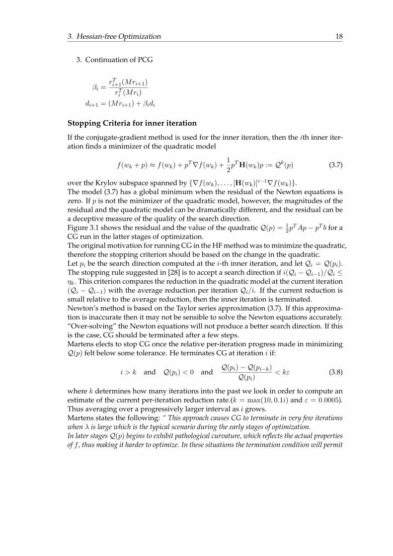
over the Krylov subspace spanned by {∇f(wk), . . . , [H(wk)]i−1∇f(wk)}.The model (3.7) has a global minimum when the residual of the Newton equations iszero. If p is not the minimizer of the quadratic model, however, the magnitudes of theresidual and the quadratic model can be dramatically different, and the residual can bea deceptive measure of the quality of the search direction.Figure 3.1 shows the residual and the value of the quadratic Q(p) = 1
2pTAp− pT b for a
CG run in the latter stages of optimization.The original motivation for running CG in the HF method was to minimize the quadratic,therefore the stopping criterion should be based on the change in the quadratic.Let pi be the search direction computed at the i-th inner iteration, and let Qi = Q(pi).The stopping rule suggested in [28] is to accept a search direction if i(Qi −Qi−1)/Qi ≤ηk. This criterion compares the reduction in the quadratic model at the current iteration(Qi − Qi−1) with the average reduction per iteration Qi/i. If the current reduction issmall relative to the average reduction, then the inner iteration is terminated.Newton’s method is based on the Taylor series approximation (3.7). If this approxima-tion is inaccurate then it may not be sensible to solve the Newton equations accurately.“Over-solving” the Newton equations will not produce a better search direction. If thisis the case, CG should be terminated after a few steps.Martens elects to stop CG once the relative per-iteration progress made in minimizingQ(p) felt below some tolerance. He terminates CG at iteration i if:
i > k and Q(pi) < 0 andQ(pi)−Q(pi−k)
Q(pi)< kε (3.8)
where k determines how many iterations into the past we look in order to compute anestimate of the current per-iteration reduction rate.(k = max(10, 0.1i) and ε = 0.0005).Thus averaging over a progressively larger interval as i grows.Martens states the following: “ This approach causes CG to terminate in very few iterationswhen λ is large which is the typical scenario during the early stages of optimization.In later stagesQ(p) begins to exhibit pathological curvature, which reflects the actual propertiesof f , thus making it harder to optimize. In these situations the termination condition will permit
3. Hessian-free Optimization 19
(a) Change of residual in a CG run (b) Change of quadraticQ(p)
Figure 3.1.: Typical behaviour of residual ‖Ax− b‖ and value of the quadratic Q(p)
CG to run much longer, resulting in a much more expensive HF iteration. But this is the pricethat seemingly must be paid.”
3.6. Preconditioning of inner iteration
The convergence of the conjugate-gradient method is strongly influenced by the condi-tion number of the Hessian (i.e., its extreme eigenvalues), and by the number of distincteigenvalues of the Hessian. Reducing either of these accelerates the convergence of themethod. Ideally, a preconditioner will be chosen based on the problem being solved.This can require considerable analysis and programming to accomplish, however, andis not suitable for routine cases. If the Hessian matrix is available, a good ’generic’choice of a preconditioner is an incomplete Cholesky factorization. The preconditioneris formed by factoring the Hessian, and ignoring some or all of the fill-in that occursduring Gaussian elimination.
Martens chooses a handmade diagonal preconditioner M :
M =
"diag
DXi=1
∇fi(θ)�∇fi(θ)!
+ λI
#α(3.9)
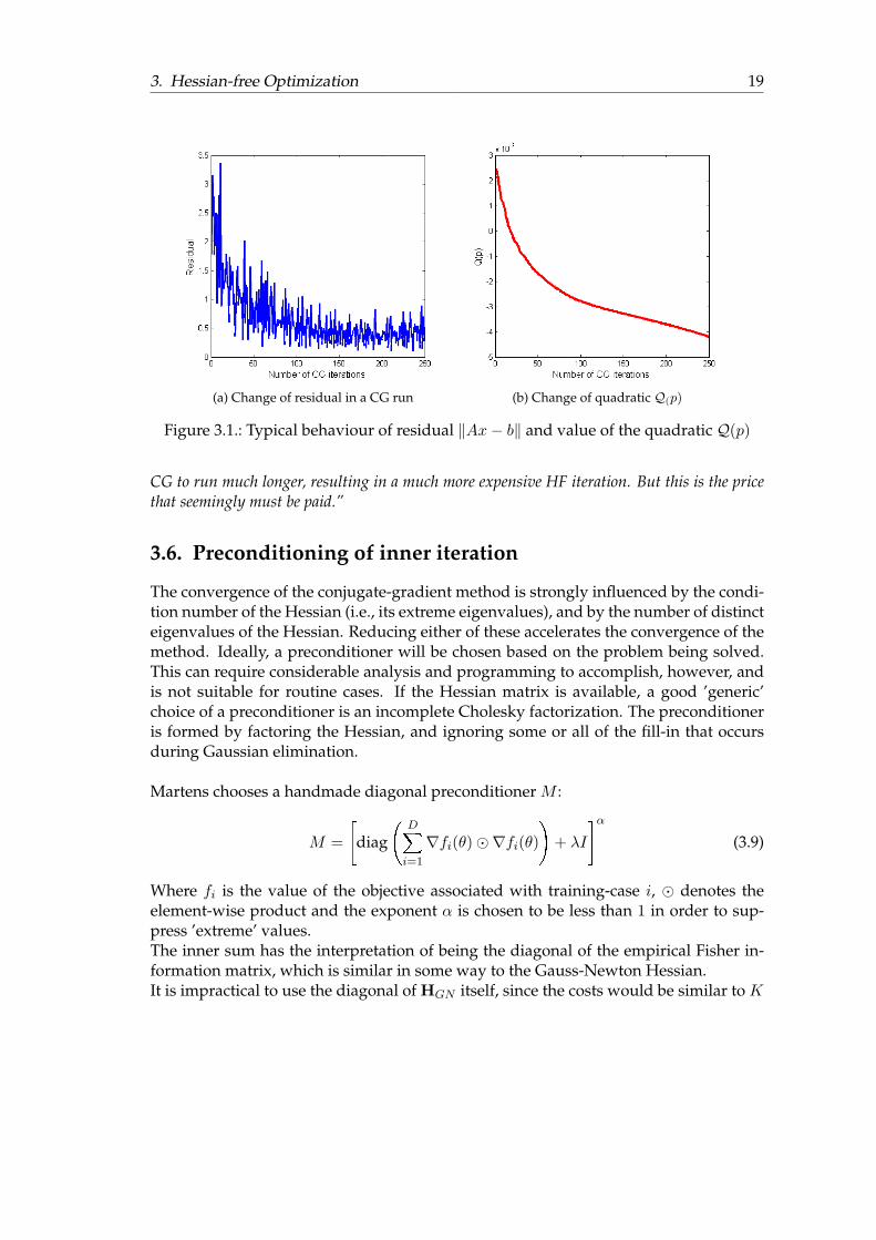
Where fi is the value of the objective associated with training-case i, � denotes theelement-wise product and the exponent α is chosen to be less than 1 in order to sup-press ’extreme’ values.The inner sum has the interpretation of being the diagonal of the empirical Fisher in-formation matrix, which is similar in some way to the Gauss-Newton Hessian.It is impractical to use the diagonal of HGN itself, since the costs would be similar to K
3. Hessian-free Optimization 20
backpropagation operations, where K is the size of the output layer, which is large forauto-encoders.
3.7. Peculiarities of Martens implementation
Computing the matrix-vector products
Pearlmutter showed that there exists an efficient procedure for computing the productHd exactly for neural networks(see [30]). Because it is similar to the backpropagationalgorithm, it involves forward and backward passes through the network and has asimilar computational cost.Schraudolph generalized Pearlmutter’s method in order to compute the Gauss-Newtonapproximation of the Hessian(see [31]).Furthermore he uses the Gauss Newton Hessian HGN instead of the Hessian H becauseit is guaranteed to be positive semi-definite thus avoiding the problem of negative cur-vature in the CG algorithm.
Sharing information across iterations
Martens uses the search direction pn−1 found by CG in the previous HF iteration asthe starting point for CG in the current one. The reasoning is that the values of H and∇f(w) for a given HF iteration should be similar in some sense to the previous ones.
Random initialization
Martens initializes the weights of the network using a sparse initialization scheme. Thenumber of non-zero incoming connection weights to each unit are hard limited andthe biases are set to 0 or 0.5 for tanh units. “Doing this allows the units to be both highlydifferentiated as well es unsaturated, avoiding the problem in dense initializations where theconnection weights must all be scaled very small in order to prevent saturation, leading to poordifferentiation between units.”
21
4. Neural networks
One common approach for modelling,e.g. using finite elements, is to write the solutiony of a PDE as a linear combination of fixed basis functions y(x,w) =
Piwiϕi(x). Al-
though this kind of models have useful analytical and computational properties, theirpractical applicability is limited by the curse of dimensionality.Using neural networks we take an alternative approach. We fix the number of basisfunctions in advance but allow them to be adaptive, in other words we use parametricforms for the basis functions in which the parameter values are adapted during train-ing.We will be following Bishop [8] and only consider feed-forward neural networks.
We first introduce the basics of neural networks.Then we focus on the construction of deep auto-encoders. The training of such an auto-encoder is used as a test-case of our preconditioner.The common algorithm used to train a feed-forward neural network is the backpropa-gation algorithm introduced in Section 4.4 .It makes use of gradient information of the error function that we try to minimize.
Truncated Newton methods like HF also need a fast procedure to efficiently calculatethe matrix vector product of the Hessian with arbitrary vectors to obtain information ofthe curvature of the error-surface. This information is needed for the inner CG iterationand are introduced in Section 4.5 .Section 4.6 shows how the Gauss-Newton Hessian is obtained for a neural network.
4.1. Feed-forward Networks
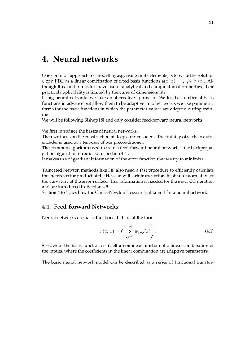
Neural networks use basic functions that are of the form
yi(x,w) = f
�MXj=1
wjϕj(x)
�. (4.1)
So each of the basis functions is itself a nonlinear function of a linear combination ofthe inputs, where the coefficients in the linear combination are adaptive parameters.
The basic neural network model can be described as a series of functional transfor-
4. Neural networks 22
mations. First M linear combinations of the input variables x1, . . . , xD in the form
aj =DXi=1
w(1)ji xi + w
(1)j0 (4.2)
are constructed, where j = 1, . . . ,M , and the superscript (1) indicates that the corrs-esponding parameters are in the first layer of the network.The parameters w(1)
ji are called weights and the parameter w(1)j0 are biases. The quanti-
ties aj are called activations.Each of them is then transformed using a differentiable, nonlinear activation functionh(·) to give
zj = h(aj). (4.3)
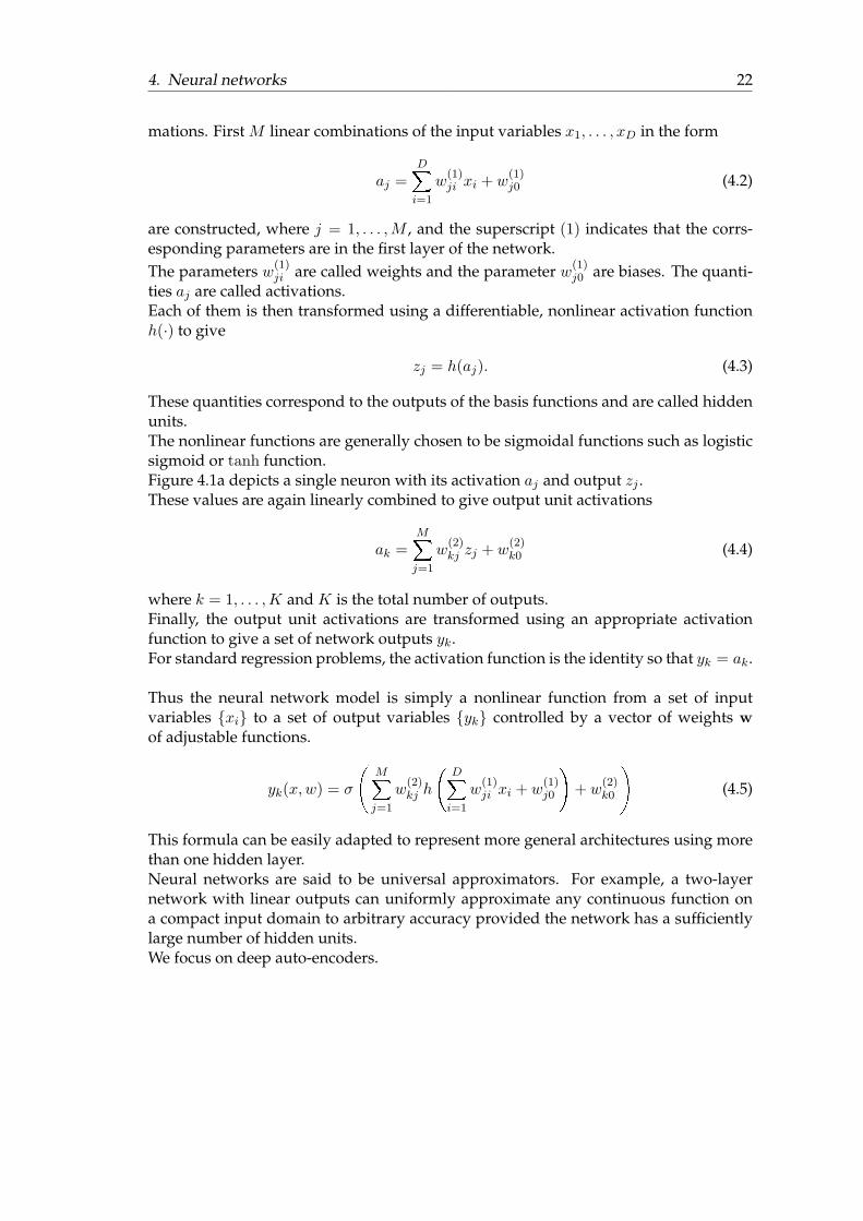
These quantities correspond to the outputs of the basis functions and are called hiddenunits.The nonlinear functions are generally chosen to be sigmoidal functions such as logisticsigmoid or tanh function.Figure 4.1a depicts a single neuron with its activation aj and output zj .These values are again linearly combined to give output unit activations
ak =MXj=1
w(2)kj zj + w
(2)k0 (4.4)
where k = 1, . . . ,K and K is the total number of outputs.Finally, the output unit activations are transformed using an appropriate activationfunction to give a set of network outputs yk.For standard regression problems, the activation function is the identity so that yk = ak.
Thus the neural network model is simply a nonlinear function from a set of inputvariables {xi} to a set of output variables {yk} controlled by a vector of weights wof adjustable functions.
yk(x,w) = σ
�MXj=1
w(2)kj h
DXi=1
w(1)ji xi + w
(1)j0
!+ w
(2)k0
�(4.5)
This formula can be easily adapted to represent more general architectures using morethan one hidden layer.Neural networks are said to be universal approximators. For example, a two-layernetwork with linear outputs can uniformly approximate any continuous function ona compact input domain to arbitrary accuracy provided the network has a sufficientlylarge number of hidden units.We focus on deep auto-encoders.
4. Neural networks 23
(a) Design of a neuron (b) Typical structure of a auto-encoder network
Figure 4.1.: Design of a singe neuron and design of an auto-encoder
4.2. Deep auto-encoder
A auto-encoder is a special feed-forward neural network of the following design.
• The input and output layers have the same size m.
• The size of the hidden layer M is smaller than m.
• The network is fully connected.
The idea is to find a compact representation of the inputs in an unsupervised mannerby letting the network recreate its own inputs and creating a bottleneck by using fewerhidden units than inputs.A given pattern x is simultaneously applied to the input layer and to the output layeras the desired response.The actual response of the output layer x is intended to be an estimate of x.By virtue of the special design of the network, the network is constrained to performidentity mapping through its hidden layer.The activations of the hidden units are then used as a compact code for x. Figure 4.1bshows an auto-encoder with a single hidden layer.
A deep auto-encoder consists of multiple hidden layers and can be thought of asa nonlinear generalization of principal component analysis (PCA) that uses an adap-tive, multilayer “encoder” network to transform the high-dimensional data into a low-dimensional code and a similar “decoder” network to recover the data from code.
Hinton and Salakhutdinov state the problem of training a deep auto-encoder as follows:“It is difficult to optimize the weights in nonlinear autoencoders that have multiple hidden lay-ers. With large initial weights, autoencoders typically find poor local minima; with small initialweights, the gradients in the early layers are tiny, making it infeasible to train autoencoders with
4. Neural networks 24
many hidden layers. If the initial weights are close to a good solution, gradient descent workswell, but finding such initial weights requires a very different type of algorithm that learns onelayer of features at a time.” (cf. [18])Thus expensive pretraining is used to come up with a good initialization for the weightsof the deep network.Martens [25] HF algorithm gives better results than the pretrained auto-encoders fordifferent test cases even though he is using a random sparse initialization scheme forthe weights. Note that the sum-of-squares reconstruction error function of a deep auto-encoder is in general non-convex and thus not easy to optimize.
4.3. Network Training
One approach to the problem of determining the network parameters w is to minimizea sum-of-squares error function. Given a training set of input vectors {xn}, where n =1, . . . , N , together with a set of corresponding target values {tn}, we minimize the errorfunction
E(w) =12
NXn = 1
‖y(xn,w)− tn‖2 . (4.6)
This is equivalent to the maximization of the likelihood function obtained for a set of Nindependent, identically distributed observations X = {x1, . . . , xN}, together with thetarget values t = {t1, . . . , tN}.
p(t|X,w, β) =NYn=1
p(tn|xn,w, β) = N (tn|y(xn,w), β−1), (4.7)
where we assumed that the target variable has a Gaussian distribution with an x-dependent mean and precision β.Taking the negative logarithm, we obtain the error function
β
2
NXn=1
{y(xn,w)− tn}2 −N
2lnβ +
N
2ln(2π). (4.8)
Maximizing the likelihood function is equivalent to minimizing the sum-of-squares er-ror function given by (4.6), where we have disregarded additive and multiplicativeconstants.Because the errorE(w) is a smooth function of w, its smallest value will occur at a pointin weight space such that the gradient of the error function vanishes.
∇E(w) = 0 (4.9)
Otherwise we could make a small step in the direction of −∇E(w) to further reducethe error.
4. Neural networks 25
Because there is no analytical solution to (4.9), iterative methods are used.Most of these techniques will update a given initial value w0 for the weight vector andthen moving through weight space in a succession of steps of the form
wk+1 = wk + ∆wk (4.10)
where k labels the iteration step.We know that making a small step into the direction of the negative gradient −∇E(w)will reduce the error. Therefore the simplest gradient based approach to reduce theerror is the update
wk+1 = wk − η∇E(w) (4.11)
where the parameter η > 0 is known as the learning rate.The error function is defined with respect to a training set, and so each step requiresthe entire training set to be processed in order to evaluate ∇E. Techniques that usethe whole data set at once are called batch methods. For batch optimization, thereare more efficient methods such as conjugate gradients, quasi-Newton or truncatedNewton methods, which are much more robust and faster than simple gradient descent.The Hessian-Free method considered in the thesis is a truncated Newton method.
4.4. Error backpropagation
We will introduce the error backpropagation algorithm. This is a local message passingscheme in which information is sent alternately forwards and backwards through thenetwork to efficiently compute the gradient∇E(w).Many error functions comprise a sum of terms, one for each data point in the trainingset, such that
E(w) =NXn=1
En(w). (4.12)
The backpropagation algorithm efficiently evaluates ∇En(w) for one such term in theerror function.
In a general feed-forward network, each unit computes a weighted sum of its inputsin the form
aj =Xi
wjizi (4.13)
where zi is the activation of a unit, that sends a connection to unit j, and wji is theweight associated with that connection. Biases can be included by introducing an extraunit, or input, with activation fixed to +1.
4. Neural networks 26
The sum in (4.13) is transformed by a nonlinear activation function h(·) to give theactivation zj of unit j in the form
zj = h(aj). (4.14)
Note that one or more of the variables zi in the sum (4.13) could be an input, and theunit j could be an output.For each pattern in the training set, we suppose that we have supplied the correspond-ing input vector to the network by successive application of (4.13) and (4.14). Thisprocess is called forward propagation.Consider the evaluation of the derivative of En with respect to a weight wji. The out-puts of the various units will depend on the particular pattern n. To keep the notationuncluttered, we omit the subscript n from the network variables.First note that En depends on wji only via the summed input aj to unit j.We apply the chain rule for partial derivatives to give
∂En∂wji
=∂En∂aj
∂aj∂wji
. (4.15)
Now set
δj :=∂En∂aj
(4.16)
where the δ’s are referred to as errors.Using (4.13), we can write
∂aj∂wji
= zi. (4.17)
Substituting (4.16) and (4.17) into (4.15), we obtain
∂En∂wji
= δjzi (4.18)
Thus the derivative is obtained simply by multiplying the value of δ for the unit at theoutput end of the weight by the value z for the unit at the input end of the weight.We only need to calculate the value δj for each hidden unit and output unit in thenetwork and then apply (4.18).For the output unit, we have
δk = yk − tk (4.19)
provided we are using the canonical link as output-unit activation function.To evalute the δ’s for hidden units, we again make use of the chain rule for partialderivatives,
δj :=∂En∂aj
=Xk
∂En∂ak
∂ak∂aj
(4.20)
4. Neural networks 27
where the sum runs over all units k to which unit j sends connections. In the aboveequation we are making use of the fact that variations in aj give rise to variations in theerror function only through variations in ak.
We obtain the backpropagation formula by substitution of the definition of δ, givenby (4.16) into (4.20), and making use of (4.13) and (4.14)
δj = h′(aj)Xk
wkjδk (4.21)
which tells us that the value of δ for a particular hidden unit can be obtained by propa-gating the δ’s backwards from units higher up in the network.
The backpropagation procedure can be summarized as follows.
Error backpropagation
1. Apply an input vector xn to the network and forward propagate through the net-work using (4.13) and (4.14) to find the activations of all the hidden units andoutput units.
2. Evaluate the δk for all output units using (4.19).
3. Backpropagate the δ’s using (4.21) to obtain δj for each hidden unit in the network.
4. Use (4.18) to evaluate the required derivatives.
For batch methods like the HF method the total error E can then be obtained by re-peating the above steps for each pattern in the training set and then summing over allpatterns:
∂E
∂wji=Xn
∂En∂wji
(4.22)
Backpropagation is able to compute the gradient∇E in O(W ), where W is the numberof all weights in the network. For example the use of a finite difference approximationwill need O(W 2).
4.5. Fast multiplication by the Hessian
The computation of the Hessian of a neural network can be expensive if the number ofweights W is large. In the context of optimization the Hessian is needed to computethe Newton direction dk = −H−1
k ∇fk in outer iteration k.Truncated Newton methods are satisified with an approximate solution of the Newtonequations Hkd
k = −∇fk.
4. Neural networks 28
This solution can be found applying a Krylov subspace method like the Conjugate Gra-dient method with a suitable stopping criterion.Therefore the Hessian is not needed, instead it suffices to be able to compute the matrix-vector product Hv for some arbitrary vectors v which are needed in the CG iterations.Pearlmutter [30] showed that the computation of these matrix vector products can becomputed efficiently in O(W ) using a variant of the backpropagation algorithm.We first note that
vTH = vT∇(∇E) (4.23)
where ∇ denotes the gradient operator in weight space. We can write down the stan-dard forward-propagation and backpropagation equations for the evaluation of ∇Eand apply (4.23) to these equations to give a set of forward-propagation and backprop-agation equations for the evaluation of vTH. This corresponds to acting on the originalequations with a differential operator vT∇. We follow Pearlmutter [30] and define theoperatorR {·} to denote the operator vT∇.The analysis makes use of the usual rules of differential calculus, together with theresult
R {w} = v. (4.24)
We will only consider a simple two-layer network with output units having linear acti-vation functions, so that yk = ak together with a sum-of-squares error.We consider the contribution of the error function for one pattern in the data set. Therequired vector is then obtained by summing over the contributions from each of thepatterns separately.The forward equations are given by
aj =Xi
wjixi (4.25)
zj = h(aj) (4.26)
yk =Xj
wkjzj (4.27)
Applying the R {·} operator to obtain a set of forward propagation equations in theform
R {aj} =Xi
vjixi (4.28)
R {zj} = h′(aj)R {aj} (4.29)
R {yk} =Xj
wkjR {zj}+Xj
vkjzj (4.30)
where vji is the element of the vector v that corresponds to the weight wji.Because we are considering a sum-of-squares error function, we have the following
4. Neural networks 29
standard backpropagation expressions:
δk = yk − tk (4.31)
δj = h′(aj)Xk
wkjδk. (4.32)
Applying theR {·} operator leads to a set of backpropagation equations in the form
R {δk} = R {yk} (4.33)
R {δj} = h′′(aj)R {aj}Xk
wkjδk + h′(aj)Xk
vkjδk + h′(aj)Xk
wkjR {δk} . (4.34)
Finally we have the usual equations for the first derivatives of the error
∂E
∂wkj= δkzj (4.35)
∂E
∂wji= δjxi (4.36)
and applyingR {·} we obtain expressions for the elements of the vector vTH
R¨∂E
∂wkj
«= R {δk} zj + δkR {zj} (4.37)
R¨∂E
∂wji
«= xiR {δj} . (4.38)
If desired, the technique can be used to evaluate the full Hessian matrix by choosingthe vector v to be given successively by a series of unit vectors, each of which picks outone column of the Hessian.
4.6. Hessian and Gauss-Newton Hessian for neural networks
Following [9], the objective function f is defined as follows. For a given example xp thej-th output unit is denoted oj(xp, w). These outputs are then combined to produce aloss. For instance, in our auto-encoder task, the sum-of-squared error can be written asPj ϕj(oj , xp), with ϕj(oj , xp) = 1
2
oj(xp, w)− xjp 2
. Commonly used loss functions canbe written in this form with ϕj a convex function.If the objective function f is of the form
f(w) =Xp
Xj
ϕj(oj(xp, w), xp), (4.39)
then the Gauss-Newton matrix HGN is defined as:
HGN =Xp
JpHp(Jp)T , with Jpij =∂oj(xp, w)
∂wiand Hp
jj =∂2ϕj(oj(xp, w), xp)
∂o2(4.40)
4. Neural networks 30
For simplicity, we have a closer look at a multilayer perceptron with a single outputneuron. Following [17], the network is trained by minimizing the cost function
Eav(w) =1
2N
NXi=1
[d(i)− F (x(i); w)]2 (4.41)
where {x(i), d(i)}Ni=1 is the training sample and F (x(i); w) is the approximating func-tion realized by the network; the weights of the network are arranged in some orderlymanner to form the weight vector w. The gradient and the Hessian of the cost functionEav(w) are respectively defined by
g(w) =∂Eav(w)∂w
(4.42)
= − 1N
NXi=1
[d(i)− F (x(i); w)]∂F (x(i); w)
∂w(4.43)
and
H(w) =∂2Eav(w)∂w2
=1N
NXi=1
�∂F (x(i); w)
∂w
� �∂F (x(i); w)
∂w
�T(4.44)
− 1N
NXi=1
[d(i)− F (x(i); w)]∂2F (x(i); w)
∂w2(4.45)
To get the Gauss-Newton approximation of the Hessian, we ignore the second term onthe right-hand side.
H(w) ≈ 1N
NXi=1
�∂F (x(i); w)
∂w
� �∂F (x(i); w)
∂w
�T(4.46)
This approximation consists of the outer product of the partial derivative ∂F (x(i);w)∂w with
itself, averaged over the training sample; accordingly, it is referred to as outer-productor Gauss-Newton approximation of the Hessian. The use of this approximation is justi-fied when the algorithm is operating in the neighborhood of a local or global minimum.Far away from a minimum the Levenberg-Marquardt parameter λ will prevent us toput too much emphasis on HGN , thus the accuracy of the approximation plays only aminor role.Schraudolph [31] showed how matrix-vector products of the Gauss-Newton Hessiancan be computed efficiently using forward and backward passes through the neuralnetwork.

31
Part III.
Construction of the SPAIPreconditioner
32
Constructing a SPAI Preconditioner for theinner iteration of the HFO Method
It should be convenient to divide the HF algorithm into two phases related to the mag-nitude of the Levenberg parameter in Hk
LM = HkGN + λI.
In Phase I because of λ� 0 the diagonal elements of HkLM will probably be the largest
elements. Thus a diagonal preconditioner like the one Martens uses should be benefi-cial.As the optimization proceeds the damping parameter λ gets smaller.If λ ≈ 0 the resulting system to be solved by the CG algorithm is the Newton equationHGNd = −∇f . where HGN is the Gauss-Newton approximation of the Hessian H.This is considered as Phase II.In this phase the Hessian is approximately as dense as in Phase I but also more shallowconsidering the magnitude of the elements.That’s why the diagonal preconditioner used in Phase I is not as beneficial as in theearlier stages to speedup the CG algorithm. Thus using a preconditioner better suitedfor the solution of a dense linear system is clearly preferable.First, we show how to obtain the needed a priori sparsity pattern for the SPAI precon-ditioner for a given matrix.Then Section 5 discusses how some easily available information about the magnitudeof the diagonal entries of the Gauss-Newton Hessian can be used to find a good sparsitypattern for M = LLT without the explicit computation of H.
Preconditioning of the CG-step
Benzi showed in [5] that a SPAI preconditioner can be used successfully to speedupGMRES even for dense matrices. This is also true for other Krylov Subspace methodslike CG.Because a SPAI preconditioner needs an a priori pattern for the inverse of A, differentapproaches to determine a good pattern are discussed. The simplest heuristic to spar-sify A is based on a threshold parameter. We use this approach to get some insight intothe pattern of H, and thus find a good pattern of H−1, at different stages of the opti-mization process. The Hessian is constructed column-wise, e.g. by constructing the jthcolumn of G by computation of the matrix-vector product HGNej where ej is the jthunit vector.
33
5. Efficient pattern finding
In his implementation of the Hessian-free optimization algorithm Martens uses the fol-lowing preconditioner:
M =
"diag
DXi=1
∂fi∂w� ∂fi∂w
!+ λI
#α(5.1)
The termDPi=1
∂fi∂w �
∂fi∂w are the diagonal entries of the empirical Fisher matrix, thus they
can be regarded as an approximation of the diagonal elements of HGN in the generalcase.Schraudolph [31] defines the Fisher information matrix FF of a scalar log-likelihoodfunction F : Rn → R as the n× n matrix formed by the outer product of its first deriva-tives.
(FF )ij =∂F(w)∂wi
· ∂F(w)∂wj
(5.2)
FF always has rank one. For more than one sample the Fisher information matrixproper is given by the expectation over all training samples, F = 〈FF 〉x. It describesthe geometric structure of weight space. For systems with a single linear output andsum-squared error, HGN reduces to F . See Schraudolph [31] for more information onthe differences between Fisher information and Gauss-Newton approximation.
Therefore Martens already computes a vector containing the approximation of the di-agonal elements of the Hessian in a vector v.
v =
0BBBBBBBBB@
Pi
�∂fi∂w1
�2...P
i
�∂fi∂wi
�2...P
i
�∂fi∂wn
�2
1CCCCCCCCCABecause of the particular pattern of the Gauss-Newton approximation of the Hessianwe can use this vector to determine an efficient sparsity pattern of our preconditioner.
5. Efficient pattern finding 34
5.1. Gauss-Newton approximation
We follow Section 4.6 and first restrict ourselves to the case of only one output neuron.Then the Gauss-Newton Hessian is given by
H(w) ≈ 1N
NXi=1
�∂F (x(i); w)
∂w
� �∂F (x(i); w)
∂w
�T. (5.3)
In more detail:
∂Fi∂w
=
�∂Fi∂w1
...∂Fi∂wn
�,
∂Fi∂w
�∂Fi∂w
�T=
�∂Fi∂w1
...∂Fi∂wn
��∂Fi∂w1
· · · ∂Fi∂wn
� X
i
∂Fi∂w
�∂Fi∂w
�T!kl
=Xi
∂Fi∂wk
∂Fi∂wl
(5.4)
Note that in the more general case with p outputs, the gradient ∂F (x(i);w)∂w has to be
substituted by the Jacobian of the p outputs. See equation (4.40) for more details.Therefore the elements
Pi∂Fi∂wk· ∂Fi∂wk
are only approximations of the real diagonal values.Nevertheless Figure 5.1 shows that using these entries already suffices to speed upGMRES.
5.2. Building the sparsity pattern
Note that in order to obtain a well-defined preconditionerM = LLT , we have to ensurethat the diagonal entries of M are nonzero.
For example consider the N -dimensional case, defining lj =Pi
�∂Fi∂wj
�2, we get
w =
�l1...lN
�.
Now we can sort this vector and only consider the products of the k largest elements.The products of these elements will have the largest values in the matrix and thusshould be the first candidates to consider when looking for a good sparsity patternfor a preconditioner.
w = sort(w) =
0BBBBBBBBB@
lill...lm...lj
1CCCCCCCCCAlm at position k
=⇒ mark positions (i, i), (l, l), (m,m), . . . , (i, l), (i,m) and (l,m).

5. Efficient pattern finding 35
(a) Exact pattern usingdroptol ε = 6.8e− 4
(b) Pattern using ∇f2 in-formation
(c) Pattern using diag(H)information
(d) Results using differentpatterns for GMRESand H40
Figure 5.1.: Exact pattern and approximations using the patternfinding idea
To get a well-defined preconditioner the diagonal entries have to be nonzero. It is con-venient to add the identity matrix.
5.3. Summary of the pattern finding method
• Set k to define the allowed sparsity of the pattern. k is the cutoff number of ele-ments in v to consider for the pattern.It is directly related to the sparsity of the pattern by k =
È(1-Sparsity%) ∗ Problemsize2.
• Compute squared gradient as approximation of the diagonal of the Hessian.Because of the particular pattern of the Gauss-Newton approximation the prod-ucts of the largest elements in this vector will tend to be the largest elements inHGN .
• Sort v and save the the k-th largest element.
• Find all elements in v that are larger than v(k).
• Find all positions where two of the k largest elements will be multiplied.
• Mark these positions in a matrix C and add the identity matrix to ensure that thepreconditioner is well-defined.
Figure 5.1a to 5.1c show the exact pattern of HGN using a predefined drop toleranceε and the approximate pattern obtained using the pattern finding algorithm mentionedabove. The results using these patterns as preconditioners for GMRES are shown in Fig-ure 5.1d. If the pattern finding method is used, the preconditioner reduces the needediterations from 300 to approximately 110. The use of the exact diagonal allows GMRESto finish after only 80 iterations.It is remarkable that the use of the pattern finding approach gives almost as good results
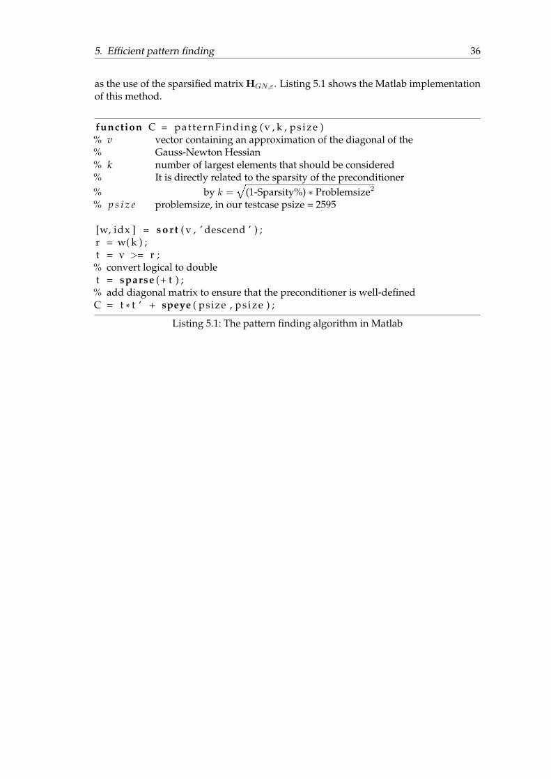
5. Efficient pattern finding 36
as the use of the sparsified matrix HGN,ε. Listing 5.1 shows the Matlab implementationof this method.
function C = patternFinding ( v , k , ps ize )% v vector containing an approximation of the diagonal of the% Gauss-Newton Hessian% k number of largest elements that should be considered% It is directly related to the sparsity of the preconditioner% by k =
È(1-Sparsity%) ∗ Problemsize2
% p s i z e problemsize, in our testcase psize = 2595
[w, idx ] = s o r t ( v , ’ descend ’ ) ;r = w( k ) ;t = v >= r ;
% convert logical to doublet = sparse (+ t ) ;
% add diagonal matrix to ensure that the preconditioner is well-definedC = t * t ’ + speye ( psize , ps ize ) ;
Listing 5.1: The pattern finding algorithm in Matlab

37
Part IV.
Case study
38
6. Training of a deep auto-encoder
6.1. Overview
The main purpose of this thesis is to apply a SPAI preconditioner in the context of op-timization using a truncated newton method by preconditioning the Krylov subspacemethod used in the inner iteration of the nonlinear optimization. It doesn’t matter ifGMRES or CG is used.Our test-case is the training of a deep auto-encoder using the HF algorithm as it is doneby Martens [26].
As dataset we use the CURVES dataset, which is an artificial dataset consisting ofgrayscale images of curves at 28 × 28 resolution. It consists of 20K training samplesand 10K testing samples. Random samples from the dataset are shown in Figure 6.2a 1.Auto-encoders are used for dimensionality reduction.See [18] for a comparison of different methods. It is trained with the objective to min-imize the reconstruction error. The activations of the smallest layer then yield an en-coded low-dimensional representation of the input. Martens code is training a deepauto-encoder using an 784-400-200-100-50-25-6 architecture for the encoding part of theneural network.This leads to about 900k weights that have to be training. The learning is done in par-allel on a GPU using Jacket2.Because of the unavailability of a Jacket license, we consider a simplified problem.
We only consider every sixteenth pixel from the input, reducing the dimensionalityof the input from 784 to 49. Then we train a deep auto-encoder with a 49-20-10-6 en-coding layer. This leads to N = 2595 weights that have to be trained.
The structure of the problem remains the same even though the input space is reduced.Therefore the results should also be applicable for the higher dimensional case usingGPUs.Through the reduction of the input space, we are able to compute the Hessian or morespecific the Gauss-Newton Hessian for some fixed HF iterations. We run the HF algo-rithm for 50 iterations.
1Figure copied from [18]2http://www.accelereyes.com/

6. Training of a deep auto-encoder 39
(a) Optimization in a long narrow valley (b) Rosenbrock function
Figure 6.1.: The Rosenbrock function as example of pathological curvature
6.2. Pathological Curvature
Before we start our analysis of the problem, it is useful to motivate the use of curvatureinformation in the optimization process. Following Martens [25], the problems associ-ated with the learning of deep neural networks like deep auto-encoder can be explainedby regions of pathological curvature in the objective function which resemble bad localminima to 1st-order optimization methods.By taking curvature into account, Newtons method rescales the gradient, so it is a muchmore sensible region to follow.If the curvature is low and positive in a particular descent direction d, the gradientchanges slowly along d. Thus d will remain a descent direction over a long distance.Therefore we should choose a search direction p that travels far along d, even if theamount of reduction associated with d, ∇fTd is relatively small.If the curvature is high, then we should choose p such that the distance traveled alongd is smaller.Newton’s method computes the distance to move along d as its reduction divided byits curvature: −∇fTd/dTHd. Not taking curvature information into account for thecomputation of the search direction can lead to undesirable scenarios:
• The sequence of search directions might constantly move to far in directions ofhigh curvature, causing the typical zig-zag path that is associated with commongradient descent methods. This can be circumvented by decreasing the learningrate.
• Directions of low curvature will be explored much more slowly than they shouldbe. Reducing the learning rate will make things worse.
• If only directions of significant decrease in f are ones of low curvature, then the
6. Training of a deep auto-encoder 40
optimization may become too slow and can appear to be trapped in a local mini-mum.
Figure 6.1a3 shows the optimization of an objective that locally resembles a long narrowvalley. At the base of the valley is a direction of low curvature and reduction that needsto be followed.The smaller black arrows show the steps taken by gradient descend with large andsmall learning rate. The red arrows are the step computed by Newton’s method.The case is pathological because of the mixture of low and high curvature directions.Figure 6.1b shows the Rosenbrock function as an example of a function that exhibitspathological curvature. A long narrow valley has to be followed to find the minimumat (0, 0).
6.3. Analysis
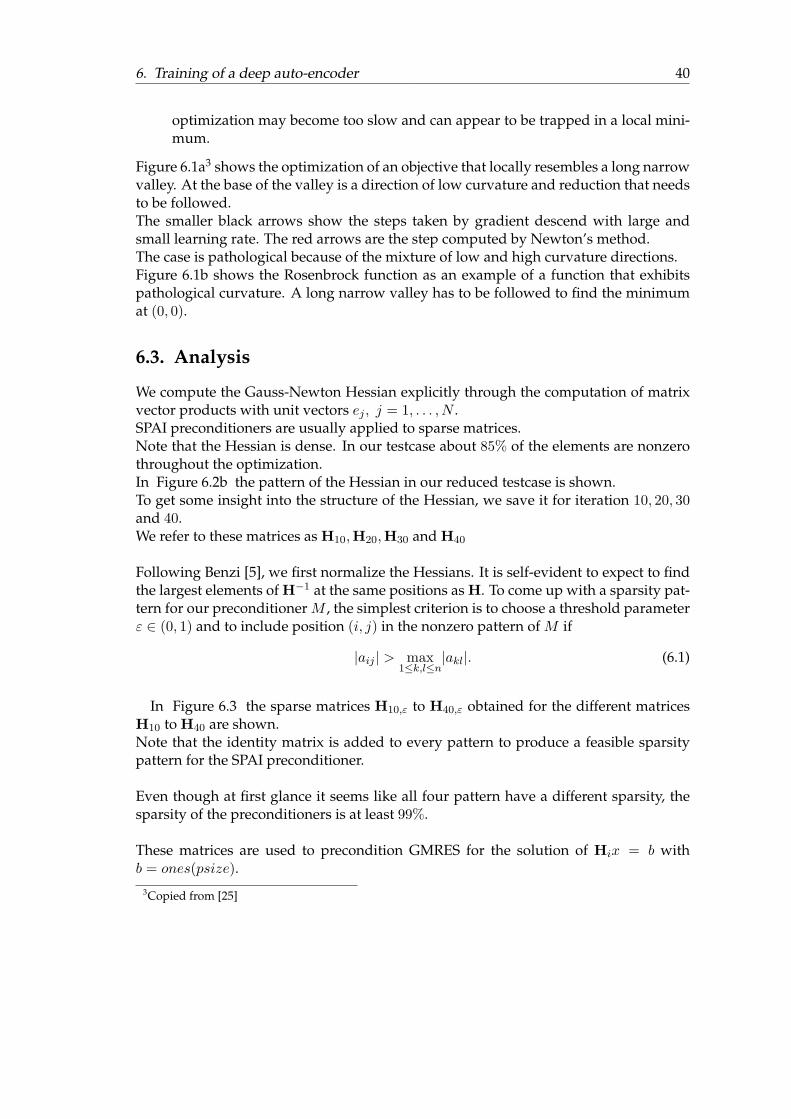
We compute the Gauss-Newton Hessian explicitly through the computation of matrixvector products with unit vectors ej , j = 1, . . . , N .SPAI preconditioners are usually applied to sparse matrices.Note that the Hessian is dense. In our testcase about 85% of the elements are nonzerothroughout the optimization.In Figure 6.2b the pattern of the Hessian in our reduced testcase is shown.To get some insight into the structure of the Hessian, we save it for iteration 10, 20, 30and 40.We refer to these matrices as H10,H20,H30 and H40
Following Benzi [5], we first normalize the Hessians. It is self-evident to expect to findthe largest elements of H−1 at the same positions as H. To come up with a sparsity pat-tern for our preconditioner M , the simplest criterion is to choose a threshold parameterε ∈ (0, 1) and to include position (i, j) in the nonzero pattern of M if
|aij | > max1≤k,l≤n
|akl|. (6.1)
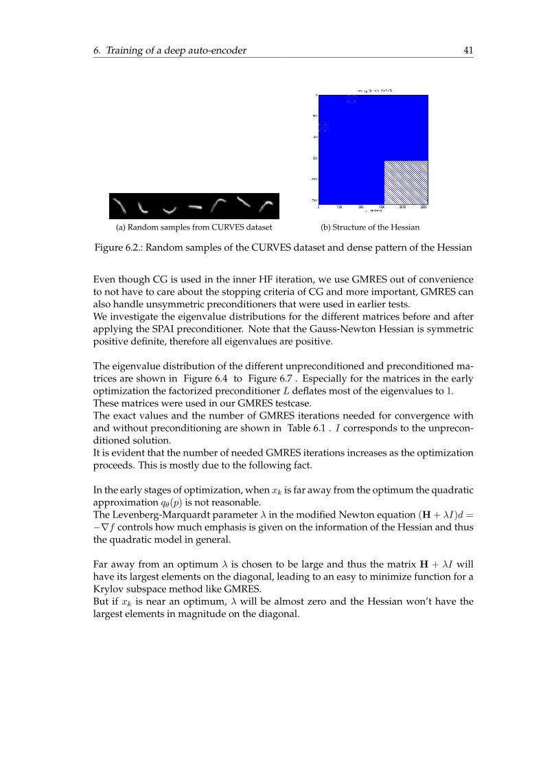
In Figure 6.3 the sparse matrices H10,ε to H40,ε obtained for the different matricesH10 to H40 are shown.Note that the identity matrix is added to every pattern to produce a feasible sparsitypattern for the SPAI preconditioner.
Even though at first glance it seems like all four pattern have a different sparsity, thesparsity of the preconditioners is at least 99%.
These matrices are used to precondition GMRES for the solution of Hix = b withb = ones(psize).
3Copied from [25]
6. Training of a deep auto-encoder 41
(a) Random samples from CURVES dataset (b) Structure of the Hessian
Figure 6.2.: Random samples of the CURVES dataset and dense pattern of the Hessian
Even though CG is used in the inner HF iteration, we use GMRES out of convenienceto not have to care about the stopping criteria of CG and more important, GMRES canalso handle unsymmetric preconditioners that were used in earlier tests.We investigate the eigenvalue distributions for the different matrices before and afterapplying the SPAI preconditioner. Note that the Gauss-Newton Hessian is symmetricpositive definite, therefore all eigenvalues are positive.
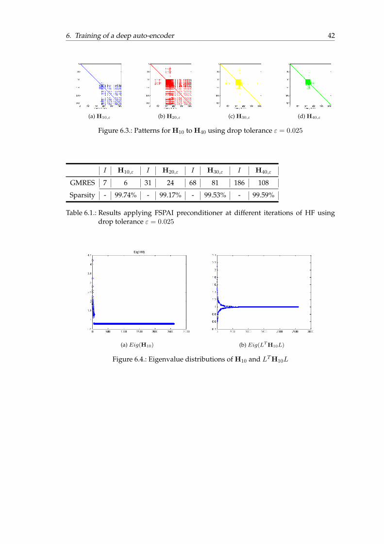
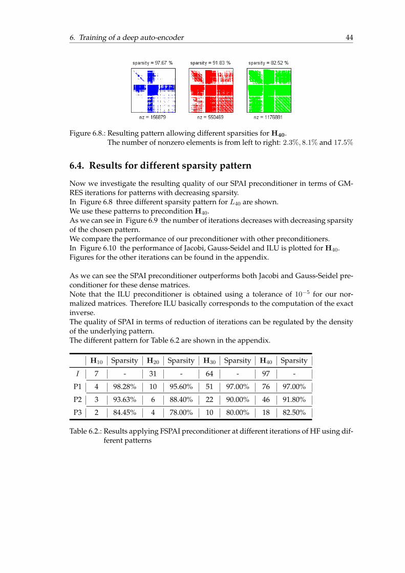
The eigenvalue distribution of the different unpreconditioned and preconditioned ma-trices are shown in Figure 6.4 to Figure 6.7 . Especially for the matrices in the earlyoptimization the factorized preconditioner L deflates most of the eigenvalues to 1.These matrices were used in our GMRES testcase.The exact values and the number of GMRES iterations needed for convergence withand without preconditioning are shown in Table 6.1 . I corresponds to the unprecon-ditioned solution.It is evident that the number of needed GMRES iterations increases as the optimizationproceeds. This is mostly due to the following fact.
In the early stages of optimization, when xk is far away from the optimum the quadraticapproximation qθ(p) is not reasonable.The Levenberg-Marquardt parameter λ in the modified Newton equation (H + λI)d =−∇f controls how much emphasis is given on the information of the Hessian and thusthe quadratic model in general.
Far away from an optimum λ is chosen to be large and thus the matrix H + λI willhave its largest elements on the diagonal, leading to an easy to minimize function for aKrylov subspace method like GMRES.But if xk is near an optimum, λ will be almost zero and the Hessian won’t have thelargest elements in magnitude on the diagonal.
6. Training of a deep auto-encoder 42
(a) H10,ε (b) H20,ε (c) H30,ε (d) H40,ε
Figure 6.3.: Patterns for H10 to H40 using drop tolerance ε = 0.025
I H10,ε I H20,ε I H30,ε I H40,ε
GMRES 7 6 31 24 68 81 186 108
Sparsity - 99.74% - 99.17% - 99.53% - 99.59%
Table 6.1.: Results applying FSPAI preconditioner at different iterations of HF usingdrop tolerance ε = 0.025
(a) Eig(H10) (b) Eig(LT H10L)
Figure 6.4.: Eigenvalue distributions of H10 and LTH10L

6. Training of a deep auto-encoder 43
(a) Eig(H20) (b) Eig(LT H20L)
Figure 6.5.: Eigenvalue distributions of H10 and LTH20L
(a) Eig(H30) (b) Eig(LT H30L)
Figure 6.6.: Eigenvalue distributions of H30 and LTH30L
(a) Eig(H40) (b) Eig(LT H40L)
Figure 6.7.: Eigenvalue distributions of H40 and LTH40L
6. Training of a deep auto-encoder 44
Figure 6.8.: Resulting pattern allowing different sparsities for H40.The number of nonzero elements is from left to right: 2.3%, 8.1% and 17.5%
6.4. Results for different sparsity pattern
Now we investigate the resulting quality of our SPAI preconditioner in terms of GM-RES iterations for patterns with decreasing sparsity.In Figure 6.8 three different sparsity pattern for L40 are shown.We use these patterns to precondition H40.As we can see in Figure 6.9 the number of iterations decreases with decreasing sparsityof the chosen pattern.We compare the performance of our preconditioner with other preconditioners.In Figure 6.10 the performance of Jacobi, Gauss-Seidel and ILU is plotted for H40.Figures for the other iterations can be found in the appendix.
As we can see the SPAI preconditioner outperforms both Jacobi and Gauss-Seidel pre-conditioner for these dense matrices.Note that the ILU preconditioner is obtained using a tolerance of 10−5 for our nor-malized matrices. Therefore ILU basically corresponds to the computation of the exactinverse.The quality of SPAI in terms of reduction of iterations can be regulated by the densityof the underlying pattern.The different pattern for Table 6.2 are shown in the appendix.
H10 Sparsity H20 Sparsity H30 Sparsity H40 Sparsity
I 7 - 31 - 64 - 97 -
P1 4 98.28% 10 95.60% 51 97.00% 76 97.00%
P2 3 93.63% 6 88.40% 22 90.00% 46 91.80%
P3 2 84.45% 4 78.00% 10 80.00% 18 82.50%
Table 6.2.: Results applying FSPAI preconditioner at different iterations of HF using dif-ferent patterns
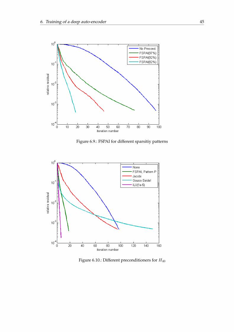
6. Training of a deep auto-encoder 45
Figure 6.9.: FSPAI for different sparsitiy patterns
Figure 6.10.: Different preconditioners for H40
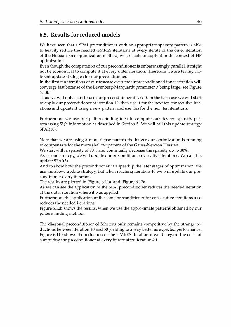
6. Training of a deep auto-encoder 46
6.5. Results for reduced models
We have seen that a SPAI preconditioner with an appropriate sparsity pattern is ableto heavily reduce the needed GMRES iterations at every iterate of the outer iterationof the Hessian-Free optimization method, we are able to apply it in the context of HFoptimization.Even though the computation of our preconditioner is embarrassingly parallel, it mightnot be economical to compute it at every outer iteration. Therefore we are testing dif-ferent update strategies for our preconditioner.In the first ten iterations of our testcase even the unpreconditioned inner iteration willconverge fast because of the Levenberg-Marquardt parameter λ being large, see Figure6.13b.Thus we will only start to use our preconditioner if λ ≈ 0. In the test-case we will startto apply our preconditioner at iteration 10, then use it for the next ten consecutive iter-ations and update it using a new pattern and use this for the next ten iterations.
Furthermore we use our pattern finding idea to compute our desired sparsity pat-tern using ∇f2 information as described in Section 5. We will call this update strategySPAI(10).
Note that we are using a more dense pattern the longer our optimization is runningto compensate for the more shallow pattern of the Gauss-Newton Hessian.We start with a sparsity of 90% and continually decrease the sparsity up to 80%.As second strategy, we will update our preconditioner every five iterations. We call thisupdate SPAI(5).And to show how the preconditioner can speedup the later stages of optimization, weuse the above update strategy, but when reaching iteration 40 we will update our pre-conditioner every iteration.The results are plotted in Figure 6.11a and Figure 6.12a .As we can see the application of the SPAI preconditioner reduces the needed iterationat the outer iteration where it was applied.Furthermore the application of the same preconditioner for consecutive iterations alsoreduces the needed iterations.Figure 6.12b shows the results, when we use the approximate patterns obtained by ourpattern finding method.
The diagonal preconditioner of Martens only remains competitive by the strange re-ductions between iteration 40 and 50 yielding to a way better as expected performance.Figure 6.11b shows the reduction of the GMRES iteration if we disregard the costs ofcomputing the preconditioner at every iterate after iteration 40.
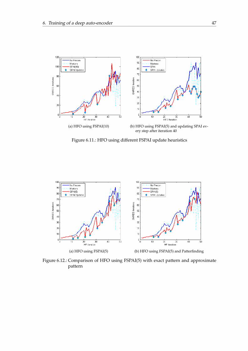
6. Training of a deep auto-encoder 47
(a) HFO using FSPAI(10) (b) HFO using FSPAI(5) and updating SPAI ev-ery step after iteration 40
Figure 6.11.: HFO using different FSPAI update heuristics
(a) HFO using FSPAI(5) (b) HFO using FSPAI(5) and Patterfinding
Figure 6.12.: Comparison of HFO using FSPAI(5) with exact pattern and approximatepattern
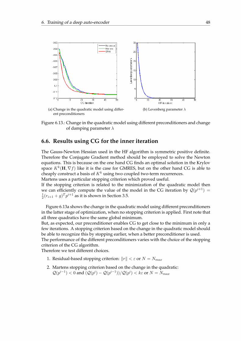
6. Training of a deep auto-encoder 48
(a) Change in the quadratic model using differ-ent preconditioners
(b) Levenberg parameter λ
Figure 6.13.: Change in the quadratic model using different preconditioners and changeof damping parameter λ
6.6. Results using CG for the inner iteration
The Gauss-Newton Hessian used in the HF algorithm is symmetric positive definite.Therefore the Conjugate Gradient method should be employed to solve the Newtonequations. This is because on the one hand CG finds an optimal solution in the Krylovspace Kk(H,∇f) like it is the case for GMRES, but on the other hand CG is able tocheaply construct a basis of Kk using two coupled two-term recurrences.Martens uses a particular stopping criterion which proved useful.If the stopping criterion is related to the minimization of the quadratic model thenwe can efficiently compute the value of the model in the CG iteration by Q(pi+1) =12(ri+1 + g)T pi+1 as it is shown in Section 3.5.
Figure 6.13a shows the change in the quadratic model using different preconditionersin the latter stage of optimization, when no stopping criterion is applied. First note thatall three quadratics have the same global minimum.But, as expected, our preconditioner enables CG to get close to the minimum in only afew iterations. A stopping criterion based on the change in the quadratic model shouldbe able to recognize this by stopping earlier, when a better preconditioner is used.The performance of the different preconditioners varies with the choice of the stoppingcriterion of the CG algorithm.Therefore we test different choices.
1. Residual-based stopping criterion: ‖r‖ < ε or N = Nmax
2. Martens stopping criterion based on the change in the quadratic:Q(pi−1) < 0 and (Q(pi)−Q(pi−1))/Q(pi) < kε or N = Nmax
6. Training of a deep auto-encoder 49
3. Combined residual- and quadratic-based stopping criteria, where the latter one isagain Martens criterion.
We use ε = 0.0005 and Nmax = 500 for all runs. Table 6.3 shows the log-likelihoodon the testset , the testset error and the total number of CG iterations needed for thedifferent runs.Note that, in practice, the number of needed CG iterations is a good measure for thetraining time of the neural network. The generalization error, defined as the error ofthe network for an unknown test set, is the most important result. Our goal was tomaximize the likelihood of our model, given the data.Note that the stopping criteria based on the residual results in a huge number of CGiterations and gives the worst results on the test set. This shows that a residual-basedstopping criteria is, in fact, a poor choice because of its divergent character.Martens stopping criterion, which is based on the change in the quadratic model, leadsto less CG iterations and better results on the test-set. This is probably because thestopping criterion forces CG to stop after only a few iterations in the beginning of theoptimization, but in later stages it permits CG to explore the regions of pathologicalcurvature that are related to small eigenvalues of the Hessian of the sum-of-squares er-ror of the network.The combined stopping criterion reduces the number of CG iterations but gives worseresults on the test-set. This is probably because sometimes a small residual forces CGto stop even though there still can be made significant progress in the optimization ofthe quadratic model.The best results are observed when using SPAI(10) and Martens stopping criterion,both, for the log-likelihood and the error on the test-case.

6. Training of a deep auto-encoder 50
Stopping Criteria Type Test Log-likelihood Testset Error Total CG Iterations
Residual SPAI(10) -4,2103 0,1588 7314
SPAI(5) -4,2216 0,1583 7472
I -4,2094 0,1609 3149
Martens -4,2023 0,1526 4523
Quadratic SPAI(10) -4,0675 0,1281 2263
SPAI(5) -4,1133 0,1394 2193
I -4,1529 0,1487 2512
Martens -4,2120 0,1546 1639
Residual/Quadratic SPAI(10) -4,1516 0,1423 1940
SPAI(5) -4,1263 0,1370 2217
I -4,1357 0,1455 2271
Martens -4,1941 0,1542 1639
Table 6.3.: HF Results using CG in the inner iteration for different stopping criteria

51
Part V.
Conclusions and Future Work

52
7. Conclusions
There are many ways to improve optimization algorithms like truncated-newton meth-ods. Other than the Newton method, truncated-Newton methods solve the Newtonequations only approximately at every outer iteration using a Krylov subspace method.Usually the positive semi-definite Gauss-Newton Hessian is used. Thus the Conju-gate Gradient algorithm is the preferred algorithm used in the inner iteration of thetruncated-Newton method.This thesis looked at the preconditioning of the inner iteration. Usually only diagonalpreconditioners are considered.We don’t restrict ourselves to diagonal preconditioning.Therefore we apply a sparse approximate inverse preconditioner(SPAI), although thistype is commonly used for sparse matrices.The most important task is to find an appropriate sparsity pattern. This is expensiveconsidering that the Hessian is only given implicitly.We use some cheaply available information about the magnitudes of the diagonal el-ements of the Hessian and the knowledge of how it is made up, to come up with aneffective procedure to construct the needed sparsity pattern for a previously fixed num-ber of nonzero elements.Furthermore we consider the test-case of training a deep auto-encoder. We analyze thestructure of the Hessian in different stages of the optimization by sparsification. Thenwe used these matrices as sparsity pattern for our SPAI preconditioner and showed theindirect relationship between the performance of our preconditioner and the sparsityof the underlying sparsity pattern.Then we compared our preconditioner with other commonly used preconditioner likeJacobi, Gauss-Seidel and ILU.We observe the superiority of our approach in terms of reductions of needed iterationsof the GMRES method.Then we’ve successfully applied our preconditioner to the training of the deep auto-encoder using different update strategies.As expected the runtime of the Krylov method used in the inner iteration is significantlydecreased at iterates where the SPAI preconditioner is applied. Furthermore even atconsecutive iterates where the same preconditioner is used, the number of needed iter-ations is still reduced.
53
8. Future Work
8.1. Parallelization of the method
One of the advantages using a sparse approximate inverse preconditioner is that itscomputation is embarrassingly parallel. Because the learning of neural networks is al-ready using the power of parallel computations on graphic cards, the actual computa-tion of a SPAI preconditioner will be faster if a better graphics card with more potentialof parallel computing is used. This can be a key aspect when considering to apply SPAIin the context of Hessian-Free optimization. In a typical SPAI implementation the pre-conditioner is computed columnwise. We need to perform W matrix-vector productswith unit vectors to compute the columns of the Hessian.If we perform this computation on one single processor the computation needs O(W )operations to compute one column of the Hessian using forward and backward passesthrough the neural network. Because of the Hessian consisting of W columns the costto compute our SPAI preconditioner needs O(W 2) operations. This clearly prohibits itsapplication on a single processor for deep networks.Nevertheless the power of SPAI lies in the great performance increase on parallel archi-tectures.
8.2. Termination of CG
There are a lot of different possibilities concerning the early termination of the CGmethod in the context of truncated-Newton methods used for nonlinear optimization.A good stopping criterion is based on the change in the quadratic model but it is alsoconnected to a forcing sequence to guarantee fast convergence [12]. Suppose we havefound a good stopping criterion, then the quality of our method will depend on thechoice how many CG iterations we allow to be done when the criterion is not satis-fied. This choice is problem dependent but it will have a huge influence in the overallpreformance of our truncated Newton method.
8.3. Application of a better approximation of the diagonal ofthe Hessian
In [9] Chapelle proposed a method to compute an unbiased estimate of the diagonal ofthe Hessian. It is shown that this Jacobi type preconditioner gives better results than
8. Future Work 54
the preconditioner Martens used. Martens preconditioner uses a more crude approxi-mation of the diagonal of the Hessian.We are using these values to compute the sparsity pattern of our preconditioner. Ofcourse the performance of our preconditioner will be increased, if we use a better ap-proximation of the diagonal values. It would be interesting to see how the performanceof the preconditioner varies using these approximations to the diagonal especially withdecreasing sparsity.Furthermore, we should use the diagonal values of the Gauss-Newton Hessian to im-prove the Levenberg-Marquardt damping, replacing HGN +λI by HGN +λdiag(HGN ).
8.4. Using more information for the preconditioner
In the process of optimization, the inner and outer loop contains information that canalso be used to produce useful preconditioners.Fassano uses information obtained while running CG to compute an appropriate pre-conditioner.“The basic idea is to deflate the eigenvalues of the matrix of the system associated with the in-variant subspace explored by the CG”(cf [15]).
8.5. Efficient calculation of particular entries of the Hessian
In its current implementation we need to compute every column of the Hessian to com-pute our preconditioner. As the computation of one column can be performed inO(W ),where W is the number of weights in the neural network, this leads to an complexity ofO(W 2) to actually compute the SPAI preconditioner. This clearly prohibits its applica-tion in a truncated-Newton method. This problem can be solved to some extend if thecomputation is performed in parallel on a graphic card.Our preconditioner is usually sparse, e.g. 95% of the elements are zero.In the columnwise computation of our preconditioner, we compute a column of theHessian, which has size W . But we only need 5% of the entries of this usually largevector.Bishop [7] showed how particular elements of the Hessian can be computed. Eventhough this method also needs O(W 2) operations to compute the full Hessian, it seemspossible to reduce the overall complexity of the computation of our preconditioner toO(W ) or O(W log(W )).An element of the Hessian is computed by a similar forward and backpropagation pro-cedure as the gradient but some additional values have to be stored.
Our pattern finding algorithm, no matter if used with the diagonal of the Fischer matrixor the real values of the Hessian, supplies us with the positions of the needed elementsin the Hessian. But if we know which elements we need to compute, then we only needto backpropagate through some part of the network. Thus we don’t compute the 95%of information that we actually don’t need for the compuation of our preconditioner.
8. Future Work 55
Furthermore we only have to calculate 12N(N + 1) elements, because of the symmetry
of the Hessian and the factorized character of our preconditioner.Therefore it seems reasonable to believe to come up with an algorithm that has a bettercomplexity than O(W 2).Suppose we have an O(W ) algorithm, then our preconditioner is perfectly suited forthe application in a truncated-Newton method that is used to train deep neural net-works.In his more recent paper Martens successfully applies his HF algorithm to train recur-rent neural networks(RNNs) [26]. These networks are known to be really hard to train.He notes that his diagonal preconditioner is not working for this kind of problems. Thisis probably due to the fact mentioned in this thesis. Diagonal preconditioners seem tobe not well suited if applied to dense matrices where a lot of elements are in the sameorder of magnitude.Our preconditioner is designed to speed up the inner iteration of the HF optimizationin this cases. This should prove extremely useful to speedup HF for the training ofRNNs.Of course, this is only true if we come up with a procedure to efficiently compute theneeded entries of the Hessian.

56
Appendix
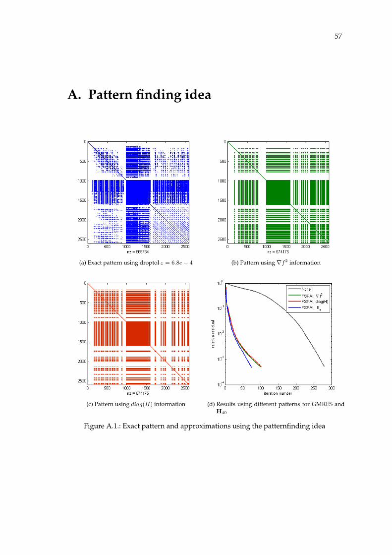
57
A. Pattern finding idea
(a) Exact pattern using droptol ε = 6.8e− 4 (b) Pattern using∇f2 information
(c) Pattern using diag(H) information (d) Results using different patterns for GMRES andH40
Figure A.1.: Exact pattern and approximations using the patternfinding idea
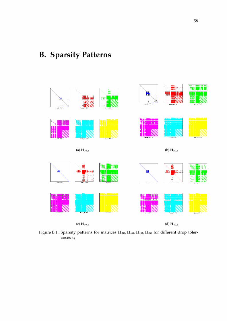
58
B. Sparsity Patterns
(a) H10,ε (b) H20,ε
(c) H30,ε (d) H40,ε
Figure B.1.: Sparsity patterns for matrices H10,H20,H30,H40 for different drop toler-ances εi
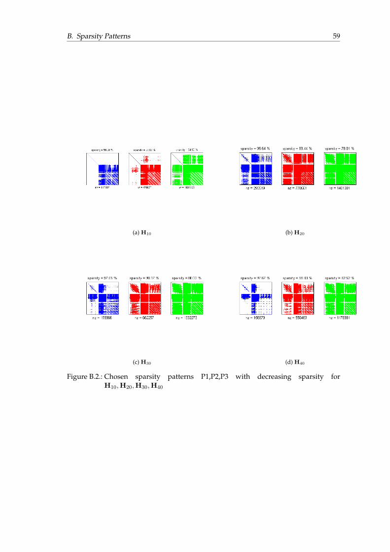
B. Sparsity Patterns 59
(a) H10 (b) H20
(c) H30 (d) H40
Figure B.2.: Chosen sparsity patterns P1,P2,P3 with decreasing sparsity forH10,H20,H30,H40
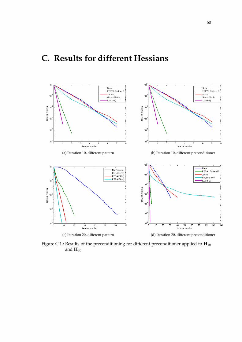
60
C. Results for different Hessians
(a) Iteration 10, different pattern (b) Iteration 10, different preconditioner
(c) Iteration 20, different pattern (d) Iteration 20, different preconditioner
Figure C.1.: Results of the preconditioning for different preconditioner applied to H10
and H20
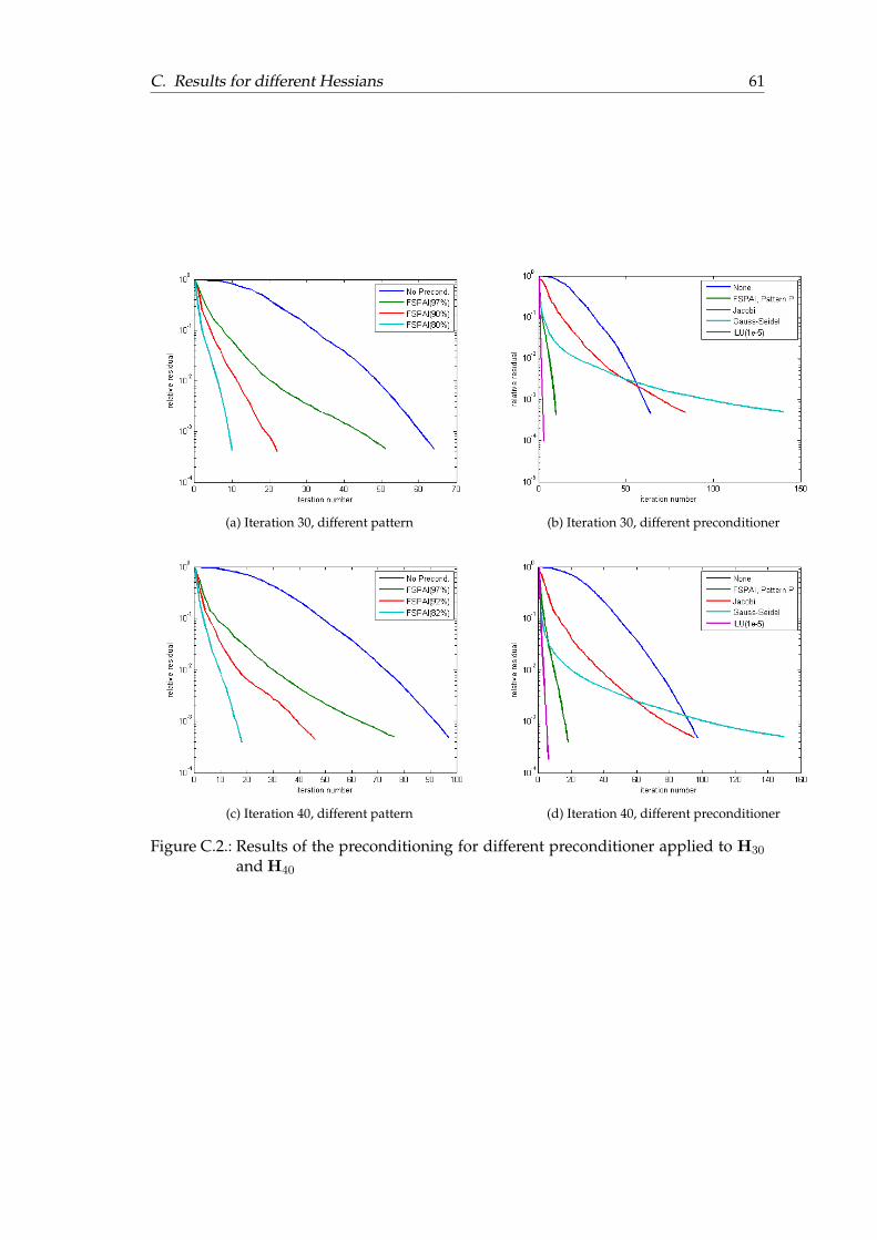
C. Results for different Hessians 61
(a) Iteration 30, different pattern (b) Iteration 30, different preconditioner
(c) Iteration 40, different pattern (d) Iteration 40, different preconditioner
Figure C.2.: Results of the preconditioning for different preconditioner applied to H30
and H40
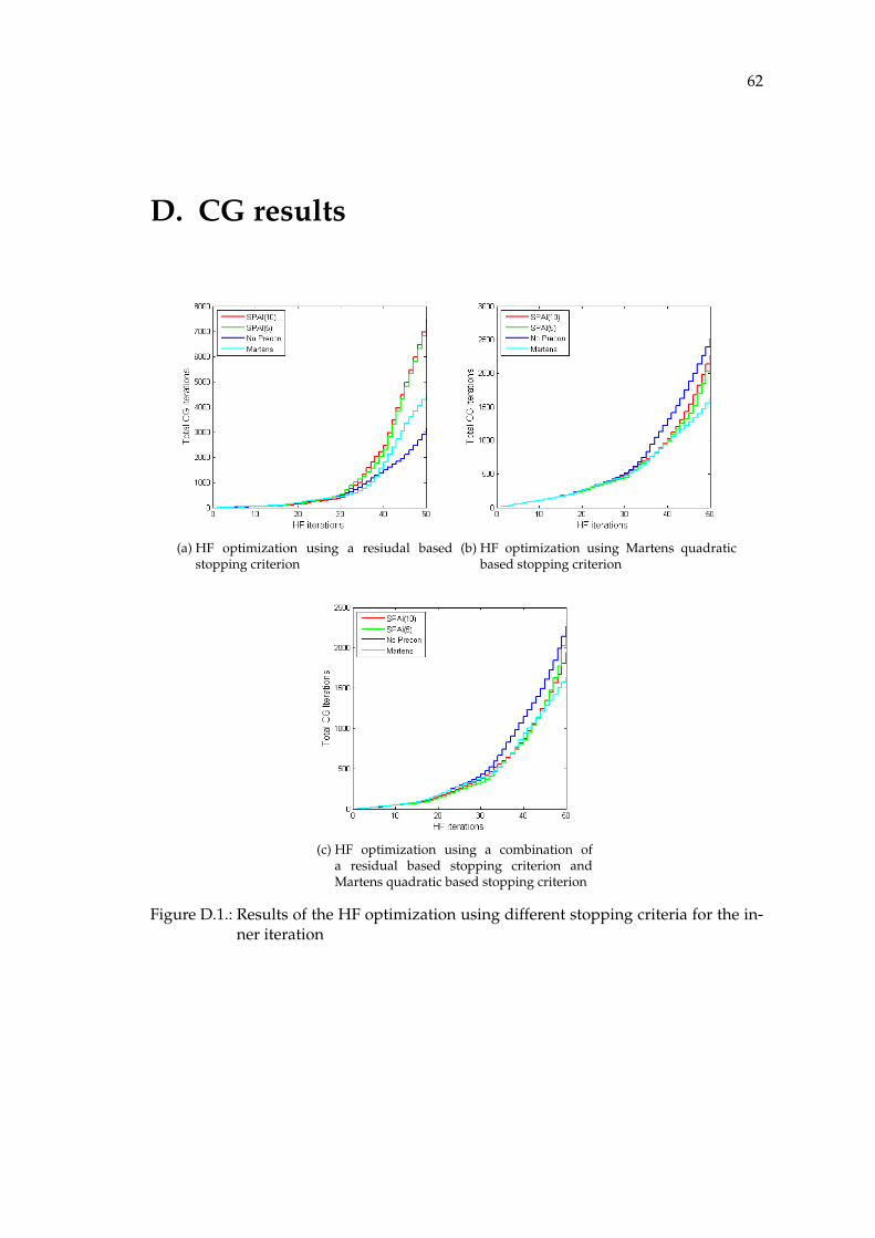
62
D. CG results
(a) HF optimization using a resiudal basedstopping criterion
(b) HF optimization using Martens quadraticbased stopping criterion
(c) HF optimization using a combination ofa residual based stopping criterion andMartens quadratic based stopping criterion
Figure D.1.: Results of the HF optimization using different stopping criteria for the in-ner iteration
63
Bibliography
[1] R. BARRETT, M. BERRY, T. F. CHAN, J. DEMMEL, J. DONATO, J. DONGARRA,V. EIJKHOUT, R. POZO, C. ROMINE, and H. V. DER VORST, Templates for theSolution of Linear Systems: Building Blocks for Iterative Methods, 2nd Edition, SIAM,Philadelphia, PA, 1994.
[2] Y. BENGIO and X. GLOROT, Understanding the difficulty of training deep feedforwardneural networks, in Proceedings of AISTATS 2010, vol. 9, May 2010, pp. 249–256.
[3] M. BENZI, Preconditioning techniques for large linear systems: a survey, J. Comput.Phys., 182, November 2002, pp. 418–477.
[4] M. BENZI, J. K. CULLUM, and M. TUMA, Robust approximate inversepreconditioning for the conjugate gradient method, SIAM J. SCI. COMPUT, 22(4),2000, pp. 1318–1332.
[5] M. BENZI, L. GIRAUD, and G. ALLEON, Sparse Approximate InversePreconditioning For Dense Linear Systems Arising In Computational Electromagnetics,Numerical Algorithms, 16, 1997, pp. 1–15.
[6] M. BENZI, C. D. MEYER, and M. TUMA, A Sparse Approximate InversePreconditioner For The Conjugate Gradient Method, SIAM J. Sci. Comput, 17, 1996,pp. 1135–1149.
[7] C. BISHOP, Exact Calculation of the Hessian Matrix for the Multilayer Perceptron,Neural Computation, 4(4), 1992, pp. 494–501.
[8] C. M. BISHOP, Pattern Recognition and Machine Learning (Information Science andStatistics), Springer, 1 ed., 2007.
[9] O. CHAPELLE and D. ERHAN, Improved Preconditioner for Hessian FreeOptimization, in NIPS Workshop on Deep Learning and Unsupervised FeatureLearning, 2011.
[10] K. CHEN, Matrix Preconditioning Techniques and Applications (CambridgeMonographs on Applied and Computational Mathematics), Cambridge UniversityPress, July 2005.
[11] P. CHEN, Hessian Matrix vs. Gauss-Newton Hessian Matrix, SIAM J. Numer. Anal.,49, July 2011, pp. 1417–1435.
[12] S. C. EISENSTAT, H. F. WALKER, S. C. EISENSTATT, HOMER, and F. WALKER,Choosing the Forcing Terms in an Inexact Newton Method, SIAM J. Sci. Comput, 17,1994, pp. 16–32.
[13] L. F. ESCUDERO, On diagonally preconditioning the truncated Newton method forsuper-scale linearly constrained nonlinear programming, European Journal ofOperational Research, 17(3), September 1984, pp. 401–414.
[14] M. FAIRBANK and E. ALONSO, Efficient Calculation of the Gauss-NewtonApproximation of the Hessian Matrix in Neural Networks, Neural Computation, 24,2012, pp. 607–610.
[15] G. FASANO and M. ROMA, An Approximate Inverse Preconditioner in TruncatedNewton Methods for Large Scale Optimization, Communications to SIMAI Congress,1(0), 2007.
[16] I. FODOR, A Survey of Dimension Reduction Techniques, tech. rep., 2002.
[17] S. HAYKIN, Neural networks and learning machines, no. Bd. 10 in Neural networksand learning machines, Prentice Hall, 2009.
[18] G. HINTON and R. SALAKHUTDINOV, Reducing the Dimensionality of Data withNeural Networks, Science, 313(5786), 2006, pp. 504 – 507.
[19] T. HUCKLE, Approximate Sparsity Patterns for the Inverse of a Matrix andPreconditioning, Applied Numerical Mathematics, 30, 1999, pp. 291–303.
[20] T. HUCKLE, Factorized Sparse Approximate Inverses for Preconditioning, J.Supercomput., 25(2), June 2003, pp. 109–117.
[21] T. HUCKLE and A. KALLISCHKO, Frobenius Norm Minimization and Probing forPreconditioning, International Journal of Computer Mathematics, 84(8), Aug. 2007,pp. 1225–1248.
[22] T. HUCKLE, A. KALLISCHKO, A. ROY, M. SEDLACEK, and T. WEINZIERL, Anefficient parallel implementation of the MSPAI preconditioner, Parallel Computing,36(5-6), 2010, pp. 273–284.
[23] Q. LE, J. NGIAM, A. COATES, A. LAHIRI, B. PROCHNOW, and A. NG, Onoptimization methods for deep learning, in Proceedings of the 28th InternationalConference on Machine Learning (ICML-11), L. Getoor and T. Scheffer, eds.,ICML ’11, New York, NY, USA, June 2011, ACM, pp. 265–272.
[24] C.-J. LIN and R. SAIGAL, An Incomplete Cholesky Factorization for Dense Matrices,Applied Numerical Mathematics, 536, p. 2000.
[25] J. MARTENS, Deep learning via Hessian-free optimization., in ICML, J. Furnkranz andT. Joachims, eds., Omnipress, 2010, pp. 735–742.
[26] J. MARTENS and I. SUTSKEVER, Learning Recurrent Neural Networks withHessian-Free Optimization, in Proceedings of the 28th International Conference onMachine Learning (ICML-11), L. Getoor and T. Scheffer, eds., ICML ’11, NewYork, NY, USA, June 2011, ACM, pp. 1033–1040.
[27] S. G. NASH, Truncated-newton methods, PhD thesis, Stanford, CA, USA, 1982.AAI8220515.
[28] S. G. NASH, A survey of truncated-Newton methods, J. Comput. Appl. Math.,124(1-2), Dec. 2000, pp. 45–59.
[29] J. NOCEDAL and S. J. WRIGHT, Numerical Optimization, Springer, New York,2nd ed., 2006.
[30] B. A. PEARLMUTTER, Fast Exact Multiplication by the Hessian, NeuralComputation, 6, 1994, pp. 147–160.
[31] N. N. SCHRAUDOLPH, Fast curvature matrix-vector products for second-ordergradient descent, Neural Comput., 14, July 2002, pp. 1723–1738.
[32] C. SIEFERT, ERIC, and D. STURLER, Probing Methods for saddle-point problems, 2005.
[33] A. VAN DER SLUIS and H. A. VAN DER VORST, The rate of convergence of conjugategradients, Numer. Math., 48(5), May 1986, pp. 543–560.
[34] O. VINYALS and D. POVEY, Krylov Subspace Descent for Deep Learning, 2011.


![Computational Science and Engineering (Int. Master’s Program) · 2013. 10. 20. · The introduction of LBM method and its history can be found in [20,22,19,21] and references therein](https://cdn.vdocuments.mx/doc/165x107/60d434ed5f57195217189597/computational-science-and-engineering-int-masteras-program-2013-10-20.jpg)


