COMPILER DESIGN OBJECTIVES:
Understand the basic concept of compiler design, and its different phases which will be helpful to construct new
tools like LEX, YACC, etc.
UNIT – I
Introduction Language Processing, Structure of a compiler the evaluation of Programming language, The Science of
building a Compiler application of Compiler Technology. Programming Language Basics.
Lexical Analysis-: The role of lexical analysis buffing, specification of tokens. Recognitions of
tokens the lexical analyzer generator lexical
UNIT –II
Syntax Analysis -: The Role of a parser, Context free Grammars Writing A grammar, top down passing bottom up
parsing Introduction to Lr Parser.
UNIT –III
More Powerful LR parser (LR1, LALR) Using Armigers Grammars Equal Recovery in Lr parser
Syntax Directed Transactions Definition, Evolution order of SDTS Application of SDTS. Syntax Directed
Translation Schemes.
UNIT – IV
Intermediated Code: Generation Variants of Syntax trees 3 Address code, Types and
Deceleration, Translation of Expressions, Type Checking. Canted Flow Back patching?
UNIT – V
Runtime Environments, Stack allocation of space, access to Non Local date on the stack Heap Management code
generation – Issues in design of code generation the target Language Address in the target code Basic blocks and
Flow graphs. A Simple Code generation.
UNIT –VI
Machine Independent Optimization. The principle sources of Optimization peep hole
Optimization, Introduction to Data flow Analysis.
OUTCOMES:
• Acquire knowledge in different phases and passes of Compiler, and specifying different
types of tokens by lexical analyzer, and also able to use the Compiler tools like LEX,
YACC, etc.
• Parser and its types i.e. Top-down and Bottom-up parsers.
• Construction of LL, SLR, CLR and LALR parse table.
• Syntax directed translation, synthesized and inherited attributes.
• Techniques for code optimization.
TEXT BOOKS:
1. Compilers, Principles Techniques and Tools.Alfred V Aho, Monical S. Lam, Ravi Sethi Jeffery D. Ullman,2nd
edition,pearson,2007
2. Compiler Design K.Muneeswaran, OXFORD
3. Principles of compiler design,2nd edition,Nandhini Prasad,Elsebier.
REFERENCE BOOKS:
1. Compiler Construction, Principles and practice, Kenneth C Louden, CENGAGE
2. Implementations of Compiler, A New approach to Compilers including the algebraic

methods, Yunlinsu ,SPRINGER
m Source pg Compiler
target
UNIT – I
Introduction Language Processing, Structure of a compiler the evaluation of Programming language, The Science of
building a Compiler application of Compiler Technology. Programming Language Basics.
Lexical Analysis-: The role of lexical analysis buffering, specification of tokens. Recognitions of tokens the lexical
analyzer generator
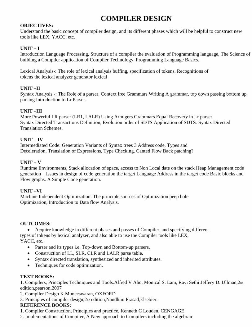
OVERVIEW OF LANGUAGE PROCESSING SYSTEM
Preprocessor A preprocessor produce input to compilers. They may perform the following functions.
1. Macro processing: A preprocessor may allow a user to define macros that are short hands for longer constructs.
2. File inclusion: A preprocessor may include header files into the program text. COMPILER
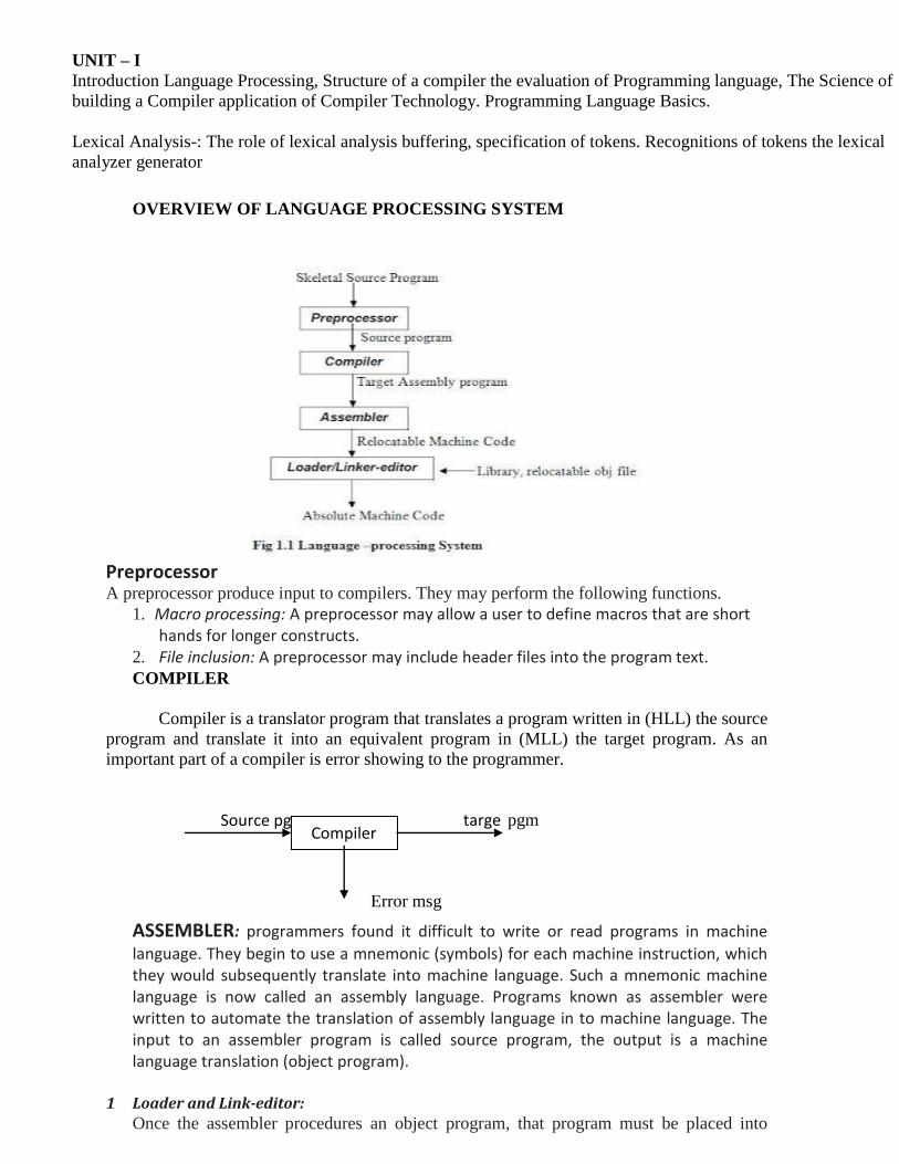
Compiler is a translator program that translates a program written in (HLL) the source
program and translate it into an equivalent program in (MLL) the target program. As an
important part of a compiler is error showing to the programmer.
pgm
Error msg
ASSEMBLER: programmers found it difficult to write or read programs in machine
language. They begin to use a mnemonic (symbols) for each machine instruction, which they would subsequently translate into machine language. Such a mnemonic machine language is now called an assembly language. Programs known as assembler were written to automate the translation of assembly language in to machine language. The input to an assembler program is called source program, the output is a machine language translation (object program).
1 Loader and Link-editor:
Once the assembler procedures an object program, that program must be placed into
memory and executed. The assembler could place the object program directly in memory
and transfer control to it, thereby causing the machine language program to be
execute. This would waste core by leaving the assembler in memory while the user’s
program was being executed. Also the programmer would have to retranslate his program
with each execution, thus wasting translation time. To over come this problems of wasted
translation time and memory. System programmers developed another component called
loader
“A loader is a program that places programs into memory and prepares them for
execution.” It would be more efficient if subroutines could be translated into object form the
loader could”relocate” directly behind the user’s program. The task of adjusting programs o
they may be placed in arbitrary core locations is called relocation. Relocation loaders
perform four functions.
STRUCTURE OF THE COMPILER DESIGN
Phases of a compiler: A compiler operates in phases. A phase is a logically interrelated
operation that takes source program in one representation and produces output in another
representation. The phases of a compiler are shown in below
There are two phases of compilation.
a. Analysis (Machine Independent/Language Dependent) b. Synthesis(Machine Dependent/Language independent)
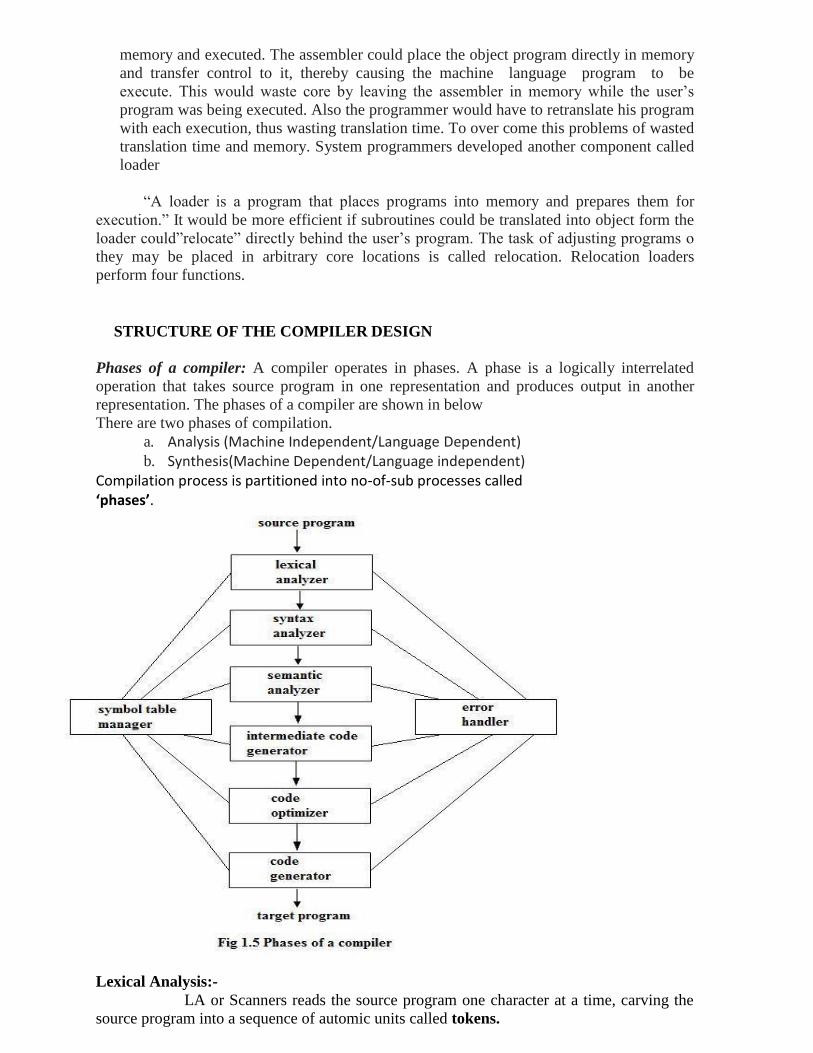
Compilation process is partitioned into no-of-sub processes called ‘phases’.
Lexical Analysis:-
LA or Scanners reads the source program one character at a time, carving the
source program into a sequence of automic units called tokens.
Syntax Analysis:-
The second stage of translation is called Syntax analysis or parsing. In this
phase expressions, statements, declarations etc… are identified by using the results of lexical
analysis. Syntax analysis is aided by using techniques based on formal grammar of the
programming language.
Intermediate Code Generations:-
An intermediate representation of the final machine language code is produced.
This phase bridges the analysis and synthesis phases of translation.
Code Optimization :-
This is optional phase described to improve the intermediate code so that the
output runs faster and takes less space.
Code Generation:-
The last phase of translation is code generation. A number of optimizations to
reduce the length of machine language program are carried out during this phase. The
output of the code generator is the machine language program of the specified computer.
Symbol Table Management
This is the portion to keep the names used by the program and records
essential information about each. The data structure used to record this information called a
‘Symbol Table’.
Error Handing :-
One of the most important functions of a compiler is the detection and
reporting of errors in the source program. The error message should allow the programmer to
determine exactly where the errors have occurred. Errors may occur in all or the phases of a
compiler.
Whenever a phase of the compiler discovers an error, it must report the error to
the error handler, which issues an appropriate diagnostic msg. Both of the table-management
and error-Handling routines interact with all phases of the compiler.
LEXICAL ANALYSIS
OVER VIEW OF LEXICAL ANALYSIS
o To identify the tokens we need some method of describing the possible tokens that can appear in the input stream. For this purpose we introduce regular expression, a notation that can be used to describe essentially all the tokens of programming language.
o Secondly , having decided what the tokens are, we need some mechanism to recognize these in the input stream. This is done by the token recognizers, which are designed using transition diagrams and finite automata.
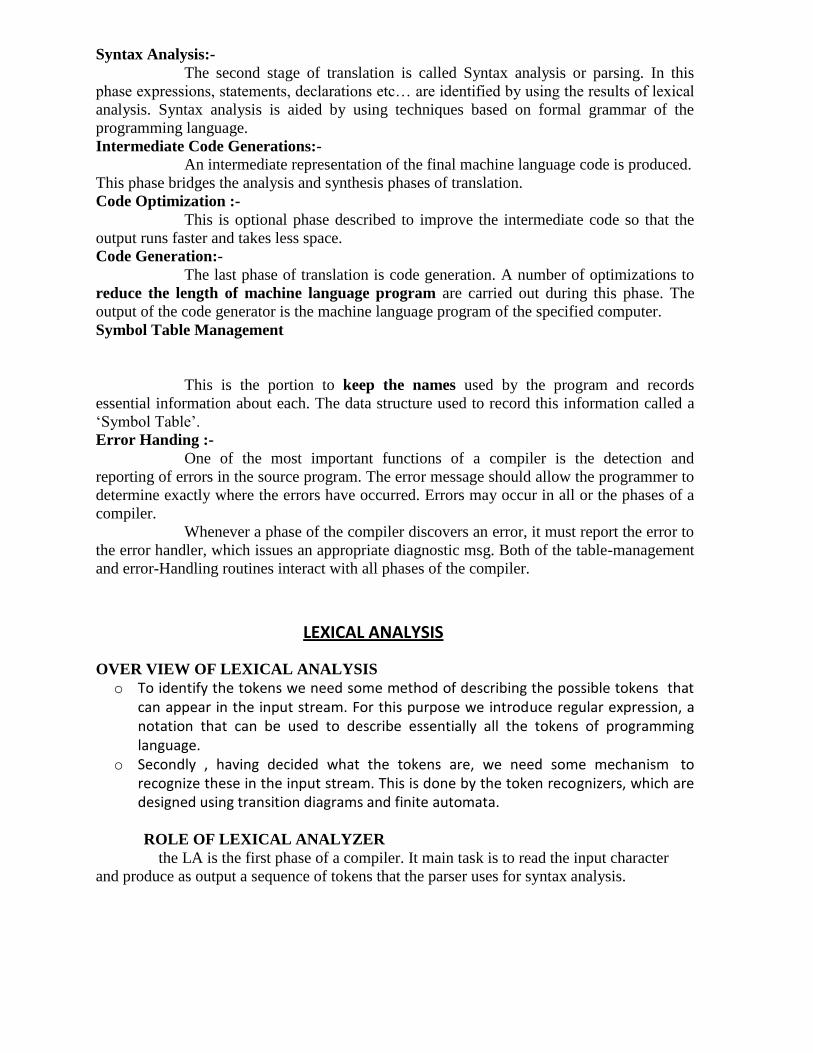
ROLE OF LEXICAL ANALYZER
the LA is the first phase of a compiler. It main task is to read the input character
and produce as output a sequence of tokens that the parser uses for syntax analysis.
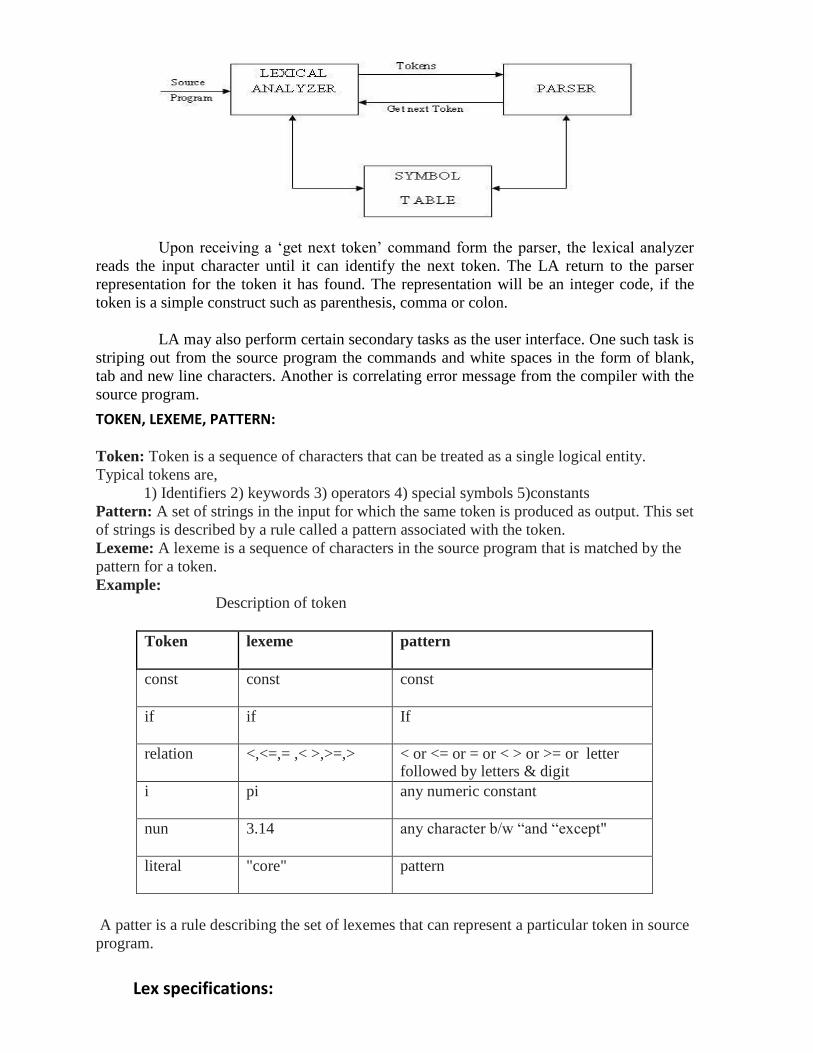
Upon receiving a ‘get next token’ command form the parser, the lexical analyzer
reads the input character until it can identify the next token. The LA return to the parser
representation for the token it has found. The representation will be an integer code, if the
token is a simple construct such as parenthesis, comma or colon.
LA may also perform certain secondary tasks as the user interface. One such task is
striping out from the source program the commands and white spaces in the form of blank,
tab and new line characters. Another is correlating error message from the compiler with the
source program.
TOKEN, LEXEME, PATTERN:
Token: Token is a sequence of characters that can be treated as a single logical entity.
Typical tokens are,
1) Identifiers 2) keywords 3) operators 4) special symbols 5)constants
Pattern: A set of strings in the input for which the same token is produced as output. This set
of strings is described by a rule called a pattern associated with the token.
Lexeme: A lexeme is a sequence of characters in the source program that is matched by the
pattern for a token.
Example:
Description of token
Token lexeme pattern
const const const
if if If
relation <,<=,= ,< >,>=,> < or <= or = or < > or >= or letter followed by letters & digit
i pi any numeric constant
nun 3.14 any character b/w “and “except"
literal "core" pattern
A patter is a rule describing the set of lexemes that can represent a particular token in source
program.
Lex specifications:
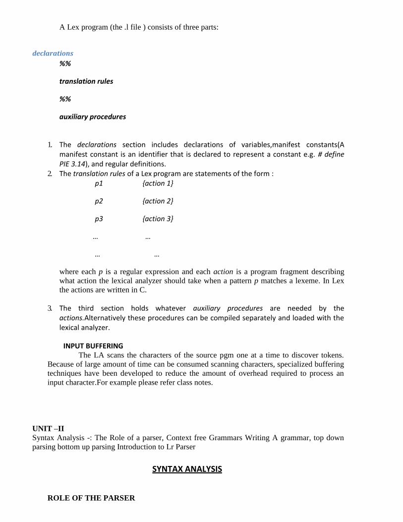
A Lex program (the .l file ) consists of three parts:
declarations
%%
translation rules
%%
auxiliary procedures
1. The declarations section includes declarations of variables,manifest constants(A
manifest constant is an identifier that is declared to represent a constant e.g. # define PIE 3.14), and regular definitions.
2. The translation rules of a Lex program are statements of the form : p1 {action 1}
p2 {action 2}
p3 {action 3}
… …
… …
where each p is a regular expression and each action is a program fragment describing
what action the lexical analyzer should take when a pattern p matches a lexeme. In Lex
the actions are written in C.
3. The third section holds whatever auxiliary procedures are needed by the actions.Alternatively these procedures can be compiled separately and loaded with the lexical analyzer.
INPUT BUFFERING
The LA scans the characters of the source pgm one at a time to discover tokens.
Because of large amount of time can be consumed scanning characters, specialized buffering
techniques have been developed to reduce the amount of overhead required to process an
input character.For example please refer class notes.
UNIT –II
Syntax Analysis -: The Role of a parser, Context free Grammars Writing A grammar, top down
parsing bottom up parsing Introduction to Lr Parser
SYNTAX ANALYSIS
ROLE OF THE PARSER
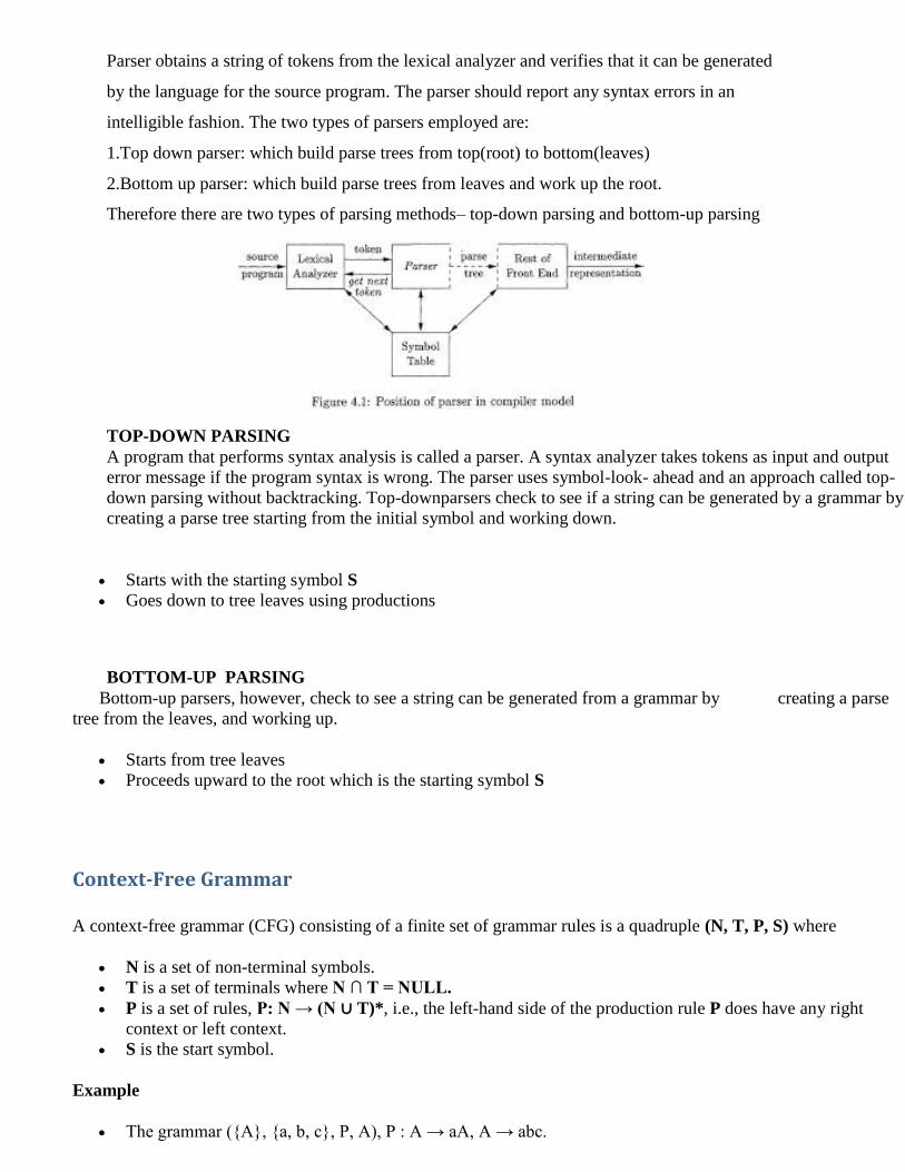
Parser obtains a string of tokens from the lexical analyzer and verifies that it can be generated
by the language for the source program. The parser should report any syntax errors in an
intelligible fashion. The two types of parsers employed are:
1.Top down parser: which build parse trees from top(root) to bottom(leaves)
2.Bottom up parser: which build parse trees from leaves and work up the root.
Therefore there are two types of parsing methods– top-down parsing and bottom-up parsing
TOP-DOWN PARSING
A program that performs syntax analysis is called a parser. A syntax analyzer takes tokens as input and output
error message if the program syntax is wrong. The parser uses symbol-look- ahead and an approach called top-
down parsing without backtracking. Top-downparsers check to see if a string can be generated by a grammar by
creating a parse tree starting from the initial symbol and working down.
• Starts with the starting symbol S
• Goes down to tree leaves using productions
BOTTOM-UP PARSING
Bottom-up parsers, however, check to see a string can be generated from a grammar by creating a parse
tree from the leaves, and working up.
• Starts from tree leaves
• Proceeds upward to the root which is the starting symbol S
Context-Free Grammar
A context-free grammar (CFG) consisting of a finite set of grammar rules is a quadruple (N, T, P, S) where
• N is a set of non-terminal symbols.
• T is a set of terminals where N ∩ T = NULL.
• P is a set of rules, P: N → (N ∪ T)*, i.e., the left-hand side of the production rule P does have any right
context or left context.
• S is the start symbol.
Example
• The grammar ({A}, {a, b, c}, P, A), P : A → aA, A → abc.
• The grammar ({S, a, b}, {a, b}, P, S), P: S → aSa, S → bSb, S → ε
• The grammar ({S, F}, {0, 1}, P, S), P: S → 00S | 11F, F → 00F | ε
Syntax analyzers follow production rules defined by means of context-free grammar. The way the production rules
are implemented (derivation) divides parsing into two types : top-down parsing and bottom-up parsing.
Top-down Parsing
When the parser starts constructing the parse tree from the start symbol and then tries to transform the start symbol
to the input, it is called top-down parsing.
• Recursive descent parsing : It is a common form of top-down parsing. It is called recursive as it uses
recursive procedures to process the input. Recursive descent parsing suffers from backtracking.
• Backtracking : It means, if one derivation of a production fails, the syntax analyzer restarts the process using
different rules of same production. This technique may process the input string more than once to determine
the right production.
Bottom-up Parsing
As the name suggests, bottom-up parsing starts with the input symbols and tries to construct the parse tree up to the
start symbol.
Example:
Input string : a + b * c
Production rules:
S → E
E → E + T
E → E * T
E → T
T → id
Let us start bottom-up parsing
a + b * c
Read the input and check if any production matches with the input:
a + b * c
T + b * c
E + b * c
E + T * c
E * c
E * T
E
S
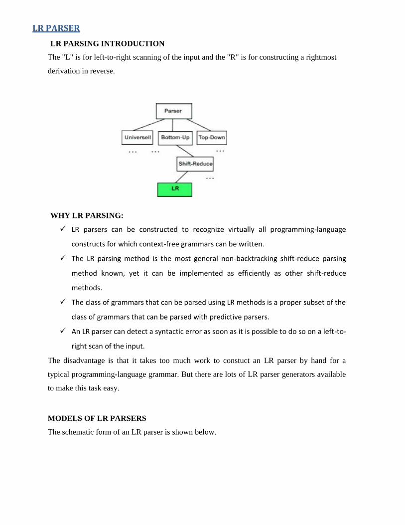
LR PARSER
LR PARSING INTRODUCTION
The "L" is for left-to-right scanning of the input and the "R" is for constructing a rightmost
derivation in reverse.
WHY LR PARSING:
✓ LR parsers can be constructed to recognize virtually all programming-language
constructs for which context-free grammars can be written.
✓ The LR parsing method is the most general non-backtracking shift-reduce parsing
method known, yet it can be implemented as efficiently as other shift-reduce
methods.
✓ The class of grammars that can be parsed using LR methods is a proper subset of the
class of grammars that can be parsed with predictive parsers.
✓ An LR parser can detect a syntactic error as soon as it is possible to do so on a left-to-
right scan of the input.
The disadvantage is that it takes too much work to constuct an LR parser by hand for a
typical programming-language grammar. But there are lots of LR parser generators available
to make this task easy.
MODELS OF LR PARSERS
The schematic form of an LR parser is shown below.
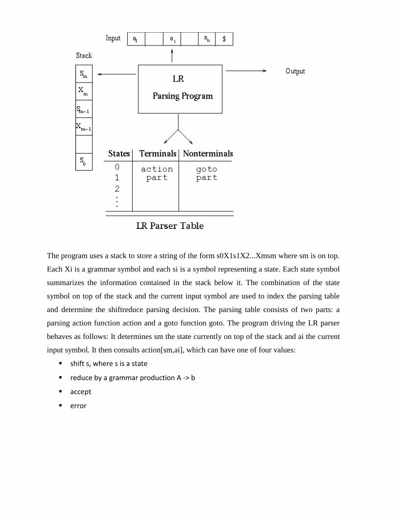
The program uses a stack to store a string of the form s0X1s1X2...Xmsm where sm is on top.
Each Xi is a grammar symbol and each si is a symbol representing a state. Each state symbol
summarizes the information contained in the stack below it. The combination of the state
symbol on top of the stack and the current input symbol are used to index the parsing table
and determine the shiftreduce parsing decision. The parsing table consists of two parts: a
parsing action function action and a goto function goto. The program driving the LR parser
behaves as follows: It determines sm the state currently on top of the stack and ai the current
input symbol. It then consults action[sm,ai], which can have one of four values:
▪ shift s, where s is a state
▪ reduce by a grammar production A -> b
▪ accept
▪ error
UNIT –III
More Powerful LR parser (LR1, LALR) Using Armigers Grammars Error Recovery in Lr parser,Syntax Directed
Transactions Definition, Evolution order of SDTS Application of SDTS. Syntax Directed Translation Schemes
ALGORITHM FOR EASY CONSTRUCTION OF AN LALR TABLE
Input: G'
Output: LALR parsing table functions with action and goto for G'.
Method:
1. Construct C = {I0, I1 , ..., In} the collection of sets of LR(1) items for G'.
2. For each core present among the set of LR(1) items, find all sets having that core
and replace these sets by the union.
3. Let C' = {J0, J1 , ..., Jm} be the resulting sets of LR(1) items. The parsing actions
for state i are constructed from Ji in the same manner as in the construction of
the canonical LR parsing table.
4. If there is a conflict, the grammar is not LALR(1) and the algorithm fails.
5. The goto table is constructed as follows: If J is the union of one or more sets of
LR(1) items, that is, J = I0U I1 U ... U Ik, then the cores of goto(I0, X), goto(I1, X),
..., goto(Ik, X) are the same, since I0, I1 , ..., Ik all have the same core. Let K be the
union of all sets of items having the same core asgoto(I1, X).
6. Then goto(J, X) = K.
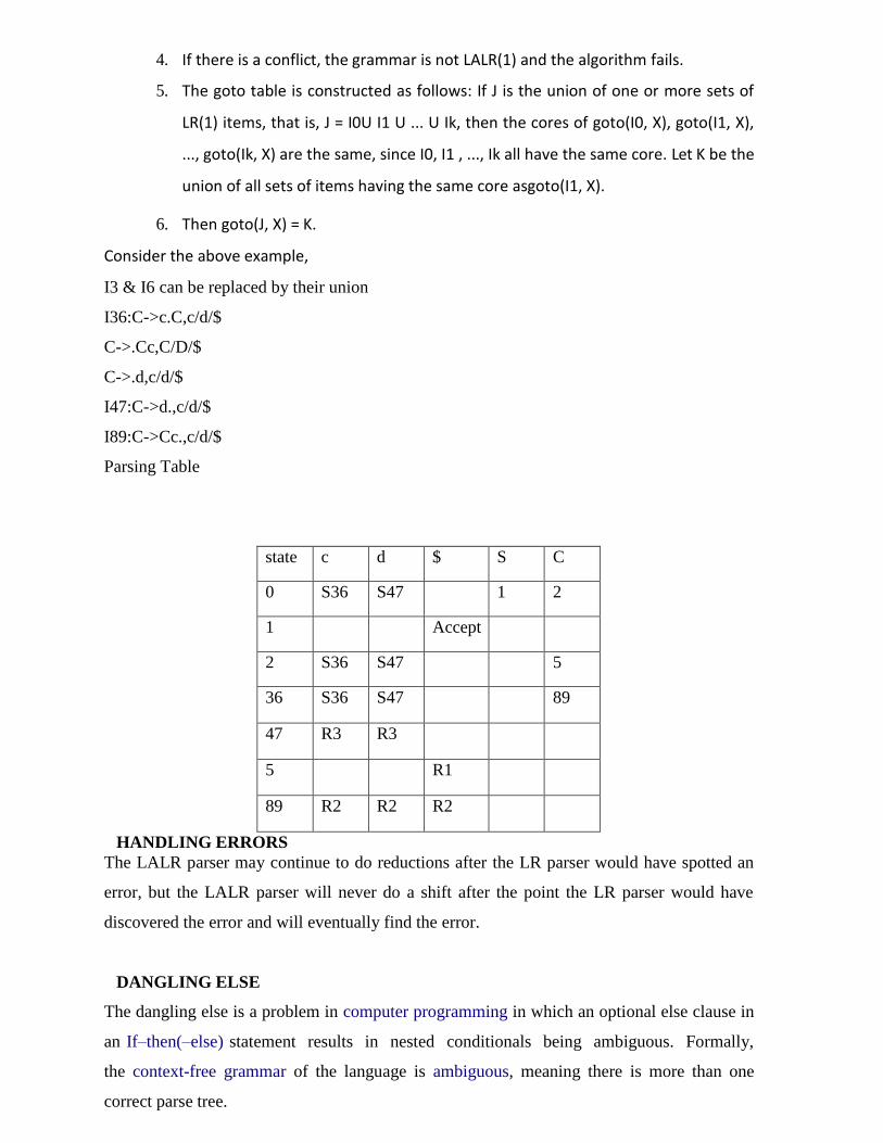
Consider the above example,
I3 & I6 can be replaced by their union
I36:C->c.C,c/d/$
C->.Cc,C/D/$
C->.d,c/d/$
I47:C->d.,c/d/$
I89:C->Cc.,c/d/$
Parsing Table
state c d $ S C
0 S36 S47 1 2
1 Accept
2 S36 S47 5
36 S36 S47 89
47 R3 R3
5 R1
89 R2 R2 R2
HANDLING ERRORS
The LALR parser may continue to do reductions after the LR parser would have spotted an
error, but the LALR parser will never do a shift after the point the LR parser would have
discovered the error and will eventually find the error.
DANGLING ELSE
The dangling else is a problem in computer programming in which an optional else clause in
an If–then(–else) statement results in nested conditionals being ambiguous. Formally,
the context-free grammar of the language is ambiguous, meaning there is more than one
correct parse tree.
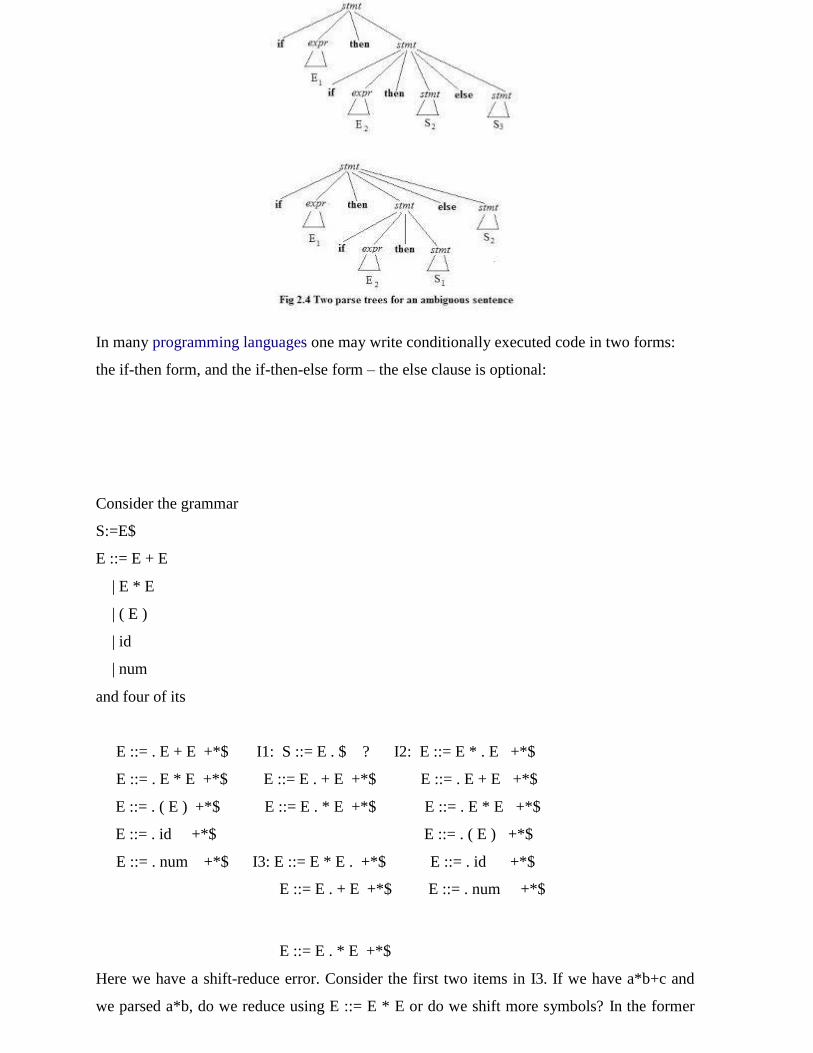
In many programming languages one may write conditionally executed code in two forms:
the if-then form, and the if-then-else form – the else clause is optional:
Consider the grammar
S:=E$
E ::= E + E
| E * E
| ( E )
| id
| num
and four of its
E ::= E . * E +*$
Here we have a shift-reduce error. Consider the first two items in I3. If we have a*b+c and
we parsed a*b, do we reduce using E ::= E * E or do we shift more symbols? In the former
E ::= . E + E +*$ I1: S ::= E . $ ? I2: E ::= E * . E +*$
E ::= . E * E +*$ E ::= E . + E +*$ E ::= . E + E +*$
E ::= . ( E ) +*$ E ::= E . * E +*$ E ::= . E * E +*$
E ::= . id +*$ E ::= . ( E ) +*$
E ::= . num +*$ I3: E ::= E * E . +*$ E ::= . id +*$
E ::= E . + E +*$ E ::= . num +*$
case we get a parse tree (a*b)+c; in the latter case we get a*(b+c). To resolve this conflict, we
can specify that * has higher precedence than +. The precedence of a grammar production is
equal to the precedence of the rightmost token at the rhs of the production. For example, the
precedence of the production E ::= E * E is equal to the precedence of the operator *, the
precedence of the production E ::= ( E ) is equal to the precedence of the token ), and the
precedence of the production E ::= if E then E else E is equal to the precedence of the token
else. The idea is that if the look ahead has higher precedence than the production currently
used, we shift. For example, if we are parsing E + E using the production rule E ::= E + E
and the look ahead is *, we shift *. If the look ahead has the same precedence as that of the
current production and is slesfotcaiative , we reduce, otherwise we shift. The above grammar
is valid if we define the precedence and associativity of all the operators. Thus, it is very
important when you write a parser using CUP or any other LALR(1) parser generator to
specify associativities and precedence’s for most tokens (especially for those used as
operators). Note: you can explicitly define the precedence of a rule in CUP using the %prec
directive:
LR ERROR RECOVERY
An LR parser will detect an error when it consults the parsing action table and find a blank or
error entry. Errors are never detected by consulting the goto table. An LR parser will detect
an error as soon as there is no valid continuation for the portion of the input thus far scanned.
A canonical LR parser will not make even
on before announcing the error.
SLR and LALR parsers may make several reductions before detecting an error, but they will
never shift an erroneous input symbol onto the stack.
PANIC-MODE ERROR RECOVERY
We can implement panic-mode error recovery by scanning down the stack until a state s with
a goto on a particular nonterminal A is found. Zero or more input symbols are then discarded
until a symbol a is found that can legitimately follow A. The parser then stacks the state
GOTO(s, A) and resumes normal parsing. The situation might exist where there is more than
one choice for the nonterminal A. Normally these would be nonterminals representing major
program pieces, e.g. an expression, a statement, or a block. For example, if A is the
nonterminal stmt, a might be semicolon or }, kwshich mar the end of a statement sequence.
This method of error recovery attempts to eliminate the phrase containing the syntactic error.
The parser determines that a string derivable from A contains an error. Part of that string has
already been processed, and the result of this processing is a sequence of states on top of the
stack. The remainder of the string is still in the input, and the parser attempts to skip over the
remainder of this string by looking for a symbol on the input that can legitimately follow A.
By removing states from the stack, skipping over the input, and pushing GOTO(s, A) on the
stack, the parser pretends that if has found an instance of A and resumes normal parsing.
PHRASE-LEVEL RECOVERY
Phrase-level recovery is implemented by examining each nertroyr e in the LR action table
and deciding on the basis of language usage the most likely programmer error that would
give rise to that error. An appropriate recovery procedure can then be constructed;
presumably the top of the stack and/or first input symbol would be modified in a way deemed
appropriate for each error entry. In designing specific error-handling routines for an LR
parser, we can fill in each blank entry in the action field with a pointer to an error routine that
will take the appropriate action selected by the compiler designer.
The actions may include insertion or deletion of symbols from the stack or the input or both,
or naldteration a transposition of input symbols. We must make our choices so that the LR
parser will not get into an infinite loop. A safe strategy will assure that at least one input
symbol will be removed or shifted eventually, or that the stack will eventually shrink if the
end of the input has been reached. Popping a stack state that covers a non terminal should be
avoided, because this modification eliminates from the stack a construct that has already been
successfully parsed.
SEMANTIC ANALYSIS
➢ Semantic Analysis computes additional information related to the meaning of the
program once the syntactic structure is known.
➢ In typed languages as C, semantic analysis involves adding information to the symbol
table and performing type checking.
➢ The information to be computed is beyond the capabilities of standard parsing
techniques, therefore it is not regarded as syntax.
➢ As for Lexical and Syntax analysis, also for Semantic Analysis we need both a
Representation Formalism and an Implementation Mechanism.
➢ As representation formalism this lecture illustrates what are called Syntax Directed
Translations.
SYNTAX DIRECTED TRANSLATION
➢ The Principle of Syntax Directed Translation states that the meaning of an input
sentence is related to its syntactic structure, i.e., to its Parse-Tree.
➢ By Syntax Directed Translations we indicate those formalisms for specifying
translations for programming language constructs guided by context-free
grammars.
o We associate Attributes to the grammar symbols representing the language
constructs.
o Values for attributes are computed by Semantic Rules associated with
grammar productions.
➢ Evaluation of Semantic Rules may:
o Generate Code;
o Insert information into the Symbol Table;
o Perform Semantic Check;
o Issue error messages;
o etc.
There are two notations for attaching semantic rules:
1. Syntax Directed Definitions. High-level specification hiding many implementation details
(also called Attribute Grammars).
2. Translation Schemes. More implementation oriented: Indicate the order in which
semantic rules are to be evaluated.
Syntax Directed Definitions
• Syntax Directed Definitions are a generalization of context-free grammars in which:
1. Grammar symbols have an associated set of Attributes;
2. Productions are associated with Semantic Rules for computing the values of attributes.
▪ Such formalism generates Annotated Parse-Trees where each node of the tree is a
record with a field for each attribute (e.g.,X.a indicates the attribute a of the
grammar symbol X).
▪ The value of an attribute of a grammar symbol at a given parse-tree node is defined
by a semantic rule associated with the production used at that node.
We distinguish between two kinds of attributes:
1. Synthesized Attributes. They are computed from the values of the attributes of the
children nodes.
2. Inherited Attributes. They are computed from the values of the attributes of both the
siblings and the parent nodes
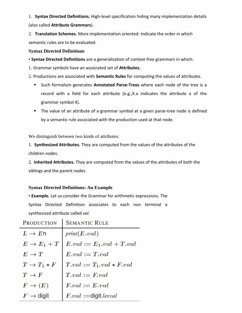
Syntax Directed Definitions: An Example
• Example. Let us consider the Grammar for arithmetic expressions. The
Syntax Directed Definition associates to each non terminal a
synthesized attribute called val.
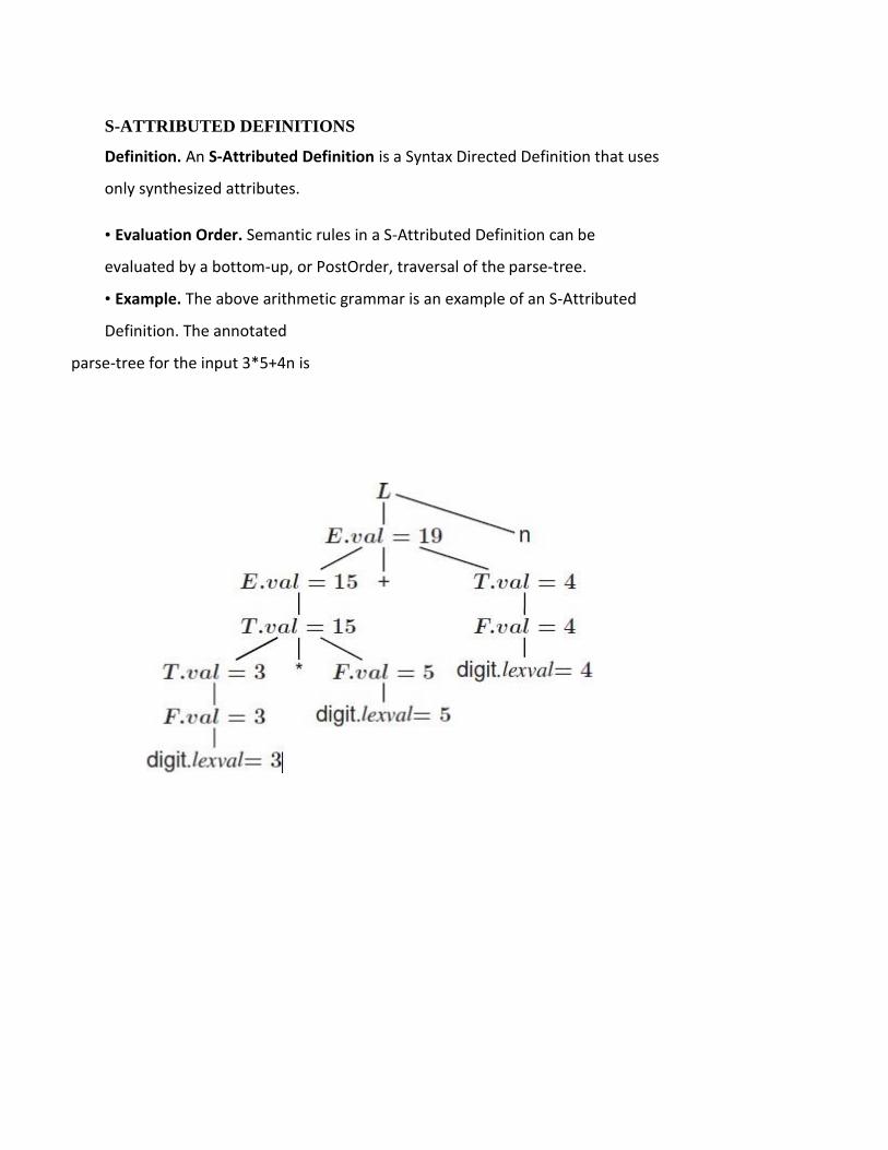
S-ATTRIBUTED DEFINITIONS
Definition. An S-Attributed Definition is a Syntax Directed Definition that uses
only synthesized attributes.
• Evaluation Order. Semantic rules in a S-Attributed Definition can be
evaluated by a bottom-up, or PostOrder, traversal of the parse-tree.
• Example. The above arithmetic grammar is an example of an S-Attributed
Definition. The annotated
parse-tree for the input 3*5+4n is
UNIT – IV
Intermediated Code: Generation Variants of Syntax trees 3 Address code, Types and
Deceleration, Translation of Expressions, Type Checking. Canted Flow Back patching
INTERMEDIATE CODE GENERATION
In the analysis-synthesis model of a compiler, the front end analyzes a source
program and creates an intermediate representation, from which the back end generates target
code. This facilitates retargeting: enables attaching a back end for the new machine to an
existing front end.
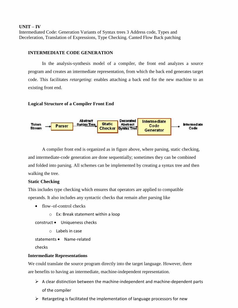
Logical Structure of a Compiler Front End
A compiler front end is organized as in figure above, where parsing, static checking,
and intermediate-code generation are done sequentially; sometimes they can be combined
and folded into parsing. All schemes can be implemented by creating a syntax tree and then
walking the tree.
Static Checking
This includes type checking which ensures that operators are applied to compatible
operands. It also includes any syntactic checks that remain after parsing like
flow–of-control checks
o Ex: Break statement within a loop
construct Uniqueness checks
o Labels in case
statements Name-related
checks
Intermediate Representations
We could translate the source program directly into the target language. However, there
are benefits to having an intermediate, machine-independent representation.
➢ A clear distinction between the machine-independent and machine-dependent parts
of the compiler
➢ Retargeting is facilitated the implementation of language processors for new
machines will require replacing only the back-end.
➢ We could apply machine independent code optimization techniques
Intermediate representations span the gap between the source and target
languages.
• High Level Representations
➢ closer to the source language
➢ easy to generate from an input program
➢ code optimizations may not be straightforward
• Low Level Representations
➢ closer to the target machine
➢ Suitable for register allocation and instruction selection
➢ easier for optimizations, final code generation
There are several options for intermediate code. They can be either
• Specific to the language being
implemented P-code for Pascal
Byte code for Java
LANGUAGE INDEPENDENT 3-ADDRESS CODE
IR can be either an actual language or a group of internal data structures that are shared by
the phases of the compiler. C used as intermediate language as it is flexible, compiles into
efficient machine code and its compilers are widely available.In all cases, the intermediate
code is a linearization of the syntax tree produced during syntax and semantic analysis. It is
formed by breaking down the tree structure into sequential instructions, each of which is
equivalent to a single, or small number of machine instructions. Machine code can then be
generated (access might be required to symbol tables etc). TAC can range from high- to low-
level, depending on the choice of operators. In general, it is a statement containing at most 3
addresses or operands.
The general form is x := y op z, where “op” is an operator, x is the result, and y and z are
operands. x, y, z are variables, constants, or “temporaries”. A three-address instruction
consists of at most 3 addresses for each statement.
It is a linear zed representation of a binary syntax tree. Explicit names correspond to interior
nodes of the graph. E.g. for a looping statement , syntax tree represents components of the
statement, whereas three-address code contains labels and jump instructions to represent the
flow-of-control as in machine language. A TAC instruction has at most one operator on the
RHS of an instruction; no built-up arithmetic expressions are permitted.
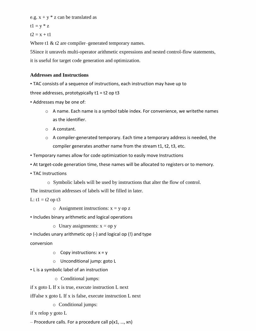
e.g. x + y * z can be translated as
t1 = y * z
t2 = x + t1
Where t1 & t2 are compiler–generated temporary names.
5Since it unravels multi-operator arithmetic expressions and nested control-flow statements,
it is useful for target code generation and optimization.
Addresses and Instructions
• TAC consists of a sequence of instructions, each instruction may have up to
three addresses, prototypically t1 = t2 op t3
• Addresses may be one of:
o A name. Each name is a symbol table index. For convenience, we writethe names
as the identifier.
o A constant.
o A compiler-generated temporary. Each time a temporary address is needed, the
compiler generates another name from the stream t1, t2, t3, etc.
• Temporary names allow for code optimization to easily move Instructions
• At target-code generation time, these names will be allocated to registers or to memory.
• TAC Instructions
o Symbolic labels will be used by instructions that alter the flow of control.
The instruction addresses of labels will be filled in later.
L: t1 = t2 op t3
o Assignment instructions: x = y op z
• Includes binary arithmetic and logical operations
o Unary assignments: x = op y
• Includes unary arithmetic op (-) and logical op (!) and type
conversion
o Copy instructions: x = y
o Unconditional jump: goto L
• L is a symbolic label of an instruction
o Conditional jumps:
if x goto L If x is true, execute instruction L next
ifFalse x goto L If x is false, execute instruction L next
o Conditional jumps:
if x relop y goto L
– Procedure calls. For a procedure call p(x1, …, xn)
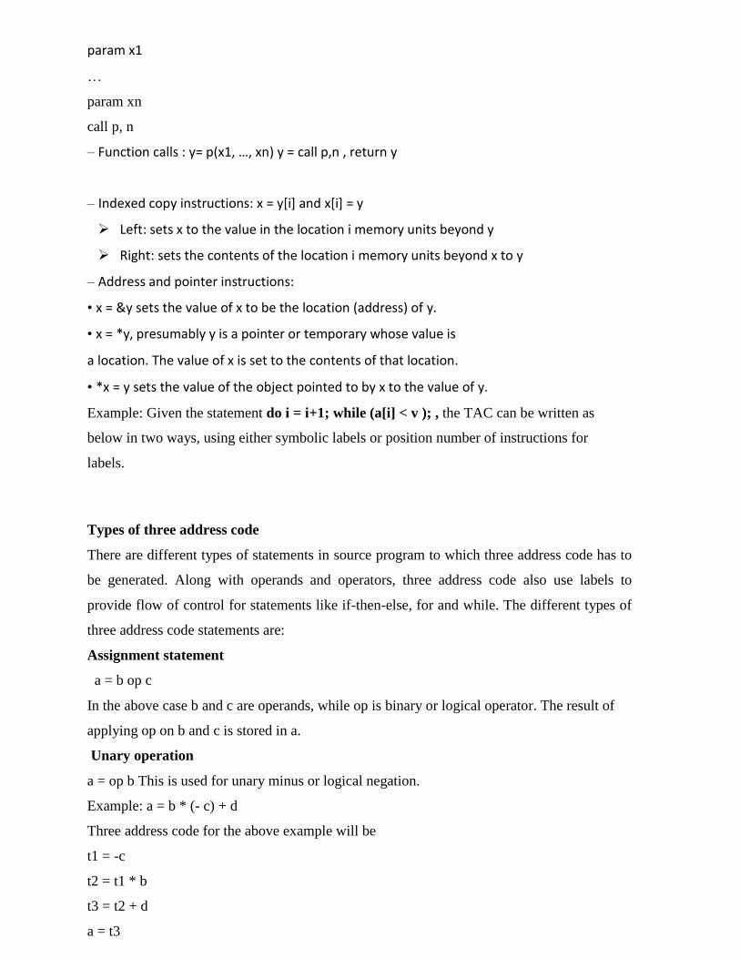
param x1
…
param xn
call p, n
– Function calls : y= p(x1, …, xn) y = call p,n , return y
– Indexed copy instructions: x = y[i] and x[i] = y
➢ Left: sets x to the value in the location i memory units beyond y
➢ Right: sets the contents of the location i memory units beyond x to y
– Address and pointer instructions:
• x = &y sets the value of x to be the location (address) of y.
• x = *y, presumably y is a pointer or temporary whose value is
a location. The value of x is set to the contents of that location.
• *x = y sets the value of the object pointed to by x to the value of y.
Example: Given the statement do i = i+1; while (a[i] < v ); , the TAC can be written as
below in two ways, using either symbolic labels or position number of instructions for
labels.
Types of three address code
There are different types of statements in source program to which three address code has to
be generated. Along with operands and operators, three address code also use labels to
provide flow of control for statements like if-then-else, for and while. The different types of
three address code statements are:
Assignment statement
a = b op c
In the above case b and c are operands, while op is binary or logical operator. The result of
applying op on b and c is stored in a.
Unary operation
a = op b This is used for unary minus or logical negation.
Example: a = b * (- c) + d
Three address code for the above example will be
t1 = -c
t2 = t1 * b
t3 = t2 + d
a = t3
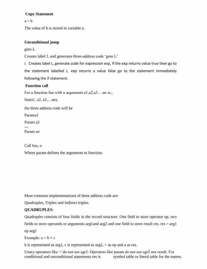
Copy Statement
a = b
The value of b is stored in variable a.
Unconditional jump
goto L
Creates label L and generates three-address code ‘goto L’
i. Creates label L, generate code for expression exp, If the exp returns value true then go to
the statement labelled L. exp returns a value false go to the statement immediately
following the if statement.
Function call
For a function fun with n arguments a1,a2,a3….an ie.,
fun(a1, a2, a3,…an),
the three address code will be
Parama1
Param a2
---
Param an
Call fun, n
Where param defines the arguments to function.
Most common implementations of three address code are-
Quadruples, Triples and Indirect triples.
QUADRUPLES-
Quadruples consists of four fields in the record structure. One field to store operator op, two
fields to store operands or arguments arg1and arg2 and one field to store result res. res = arg1
op arg2
Example: a = b + c
b is represented as arg1, c is represented as arg2, + as op and a as res.
Unary operators like ‘-‘do not use agr2. Operators like param do not use agr2 nor result. For
conditional and unconditional statements res is symbol table or literal table for the names.

Example: a = -b * d + c + (-b) * d
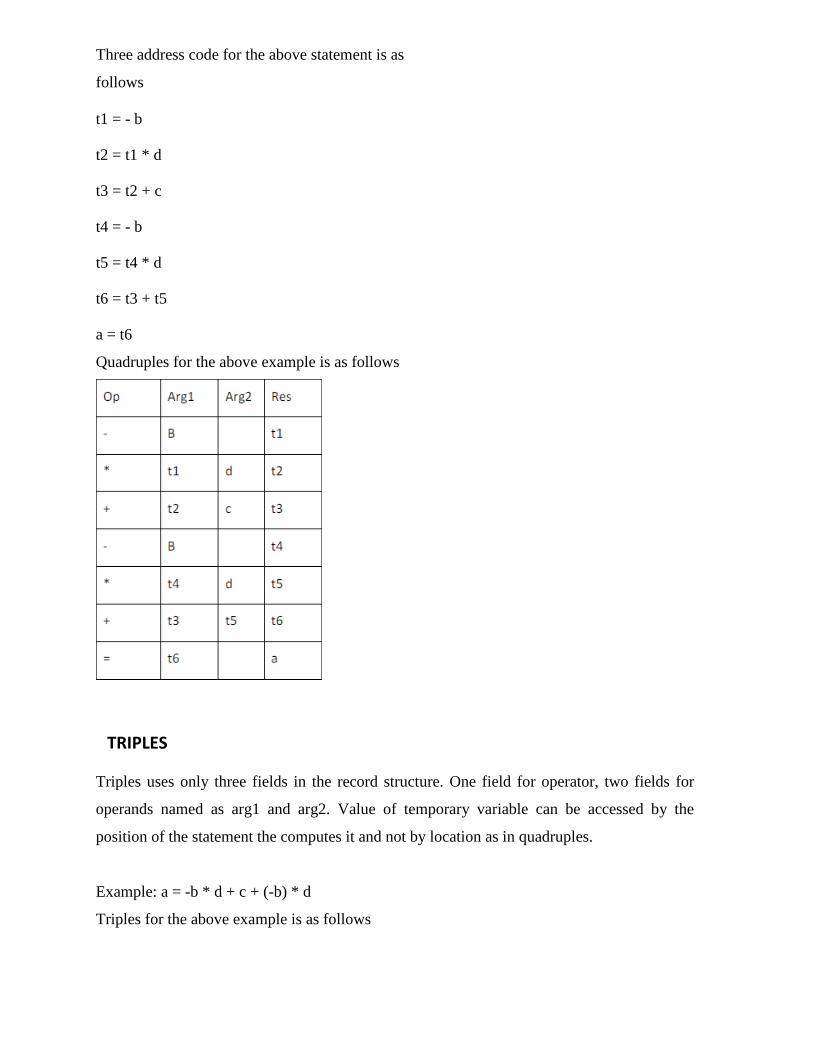
Three address code for the above statement is as
follows
t1 = - b
t2 = t1 * d
t3 = t2 + c
t4 = - b
t5 = t4 * d
t6 = t3 + t5
a = t6
Quadruples for the above example is as follows
TRIPLES
Triples uses only three fields in the record structure. One field for operator, two fields for
operands named as arg1 and arg2. Value of temporary variable can be accessed by the
position of the statement the computes it and not by location as in quadruples.
Example: a = -b * d + c + (-b) * d
Triples for the above example is as follows
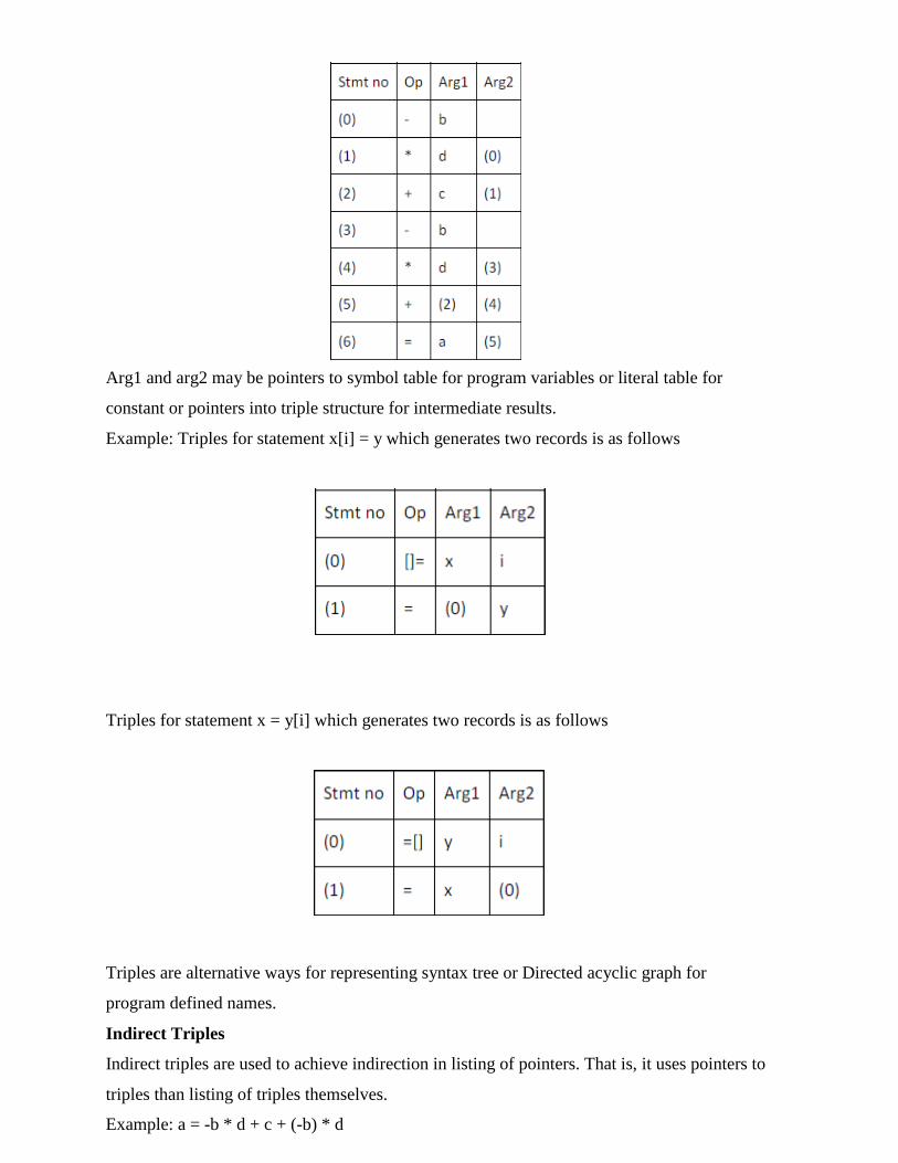
Arg1 and arg2 may be pointers to symbol table for program variables or literal table for
constant or pointers into triple structure for intermediate results.
Example: Triples for statement x[i] = y which generates two records is as follows
Triples for statement x = y[i] which generates two records is as follows
Triples are alternative ways for representing syntax tree or Directed acyclic graph for
program defined names.
Indirect Triples
Indirect triples are used to achieve indirection in listing of pointers. That is, it uses pointers to
triples than listing of triples themselves.
Example: a = -b * d + c + (-b) * d
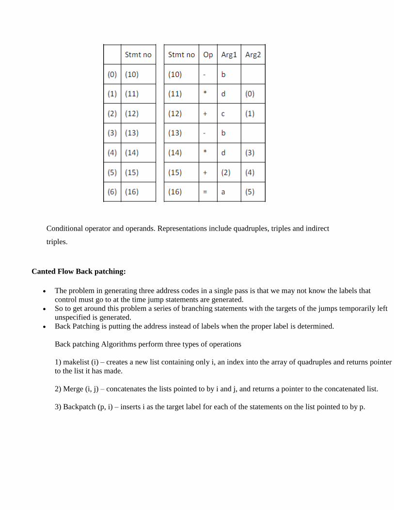
Conditional operator and operands. Representations include quadruples, triples and indirect
triples.
Canted Flow Back patching:
• The problem in generating three address codes in a single pass is that we may not know the labels that
control must go to at the time jump statements are generated.
• So to get around this problem a series of branching statements with the targets of the jumps temporarily left
unspecified is generated.
• Back Patching is putting the address instead of labels when the proper label is determined.
Back patching Algorithms perform three types of operations
1) makelist (i) – creates a new list containing only i, an index into the array of quadruples and returns pointer
to the list it has made.
2) Merge (i, j) – concatenates the lists pointed to by i and j, and returns a pointer to the concatenated list.
3) Backpatch (p, i) – inserts i as the target label for each of the statements on the list pointed to by p.
UNIT – V
Runtime Environments, Stack allocation of space, access to Non Local data on the stack Heap Management code
generation – Issues in design of code generation the target Language Address in the target code Basic blocks and
Flow graphs. A Simple Code generation.
RUNTIME ENVIRONMENT
➢ Runtime organization of different storage locations
➢ Representation of scopes and extents during program execution.
➢ Components of executing program reside in blocks of memory (supplied by OS).
➢ Three kinds of entities that need to be managed at runtime:
o Generated code for various procedures and programs.
forms text or code segment of your program: size known at compile time.
o Data objects:
Global variables/constants: size known at compile time
Variables declared within procedures/blocks: size known
Variables created dynamically: size unknown.
Stack to keep track of procedure activations. Subdivide
memory conceptually into code and data areas:
Code: Program
Instructions
Stack: Manage activation of procedures at runtime. Heap: holds variables created dynamically
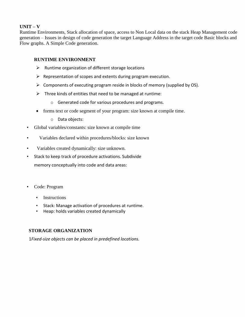
STORAGE ORGANIZATION
1Fixed-size objects can be placed in predefined locations.
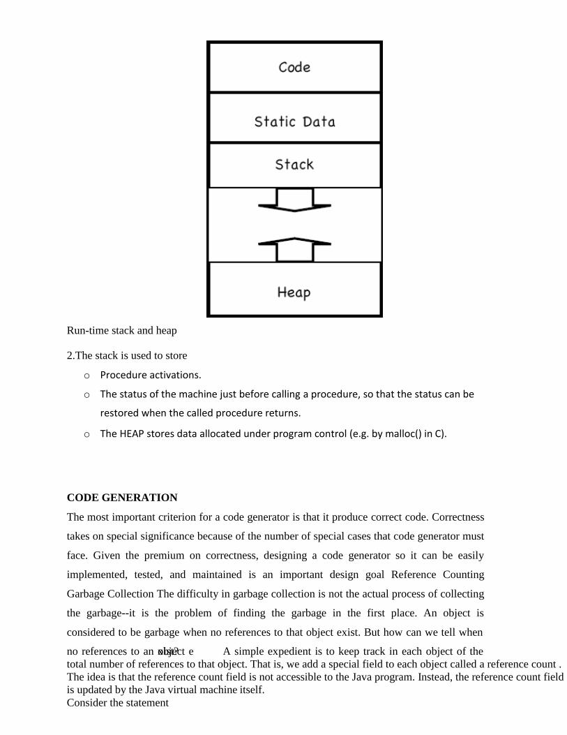
Run-time stack and heap
2.The stack is used to store
o Procedure activations.
o The status of the machine just before calling a procedure, so that the status can be
restored when the called procedure returns.
o The HEAP stores data allocated under program control (e.g. by malloc() in C).
CODE GENERATION
The most important criterion for a code generator is that it produce correct code. Correctness
takes on special significance because of the number of special cases that code generator must
face. Given the premium on correctness, designing a code generator so it can be easily
implemented, tested, and maintained is an important design goal Reference Counting
Garbage Collection The difficulty in garbage collection is not the actual process of collecting
the garbage--it is the problem of finding the garbage in the first place. An object is
considered to be garbage when no references to that object exist. But how can we tell when
no references to an xobisjte?ct e A simple expedient is to keep track in each object of the
total number of references to that object. That is, we add a special field to each object called a reference count .
The idea is that the reference count field is not accessible to the Java program. Instead, the reference count field
is updated by the Java virtual machine itself.
Consider the statement
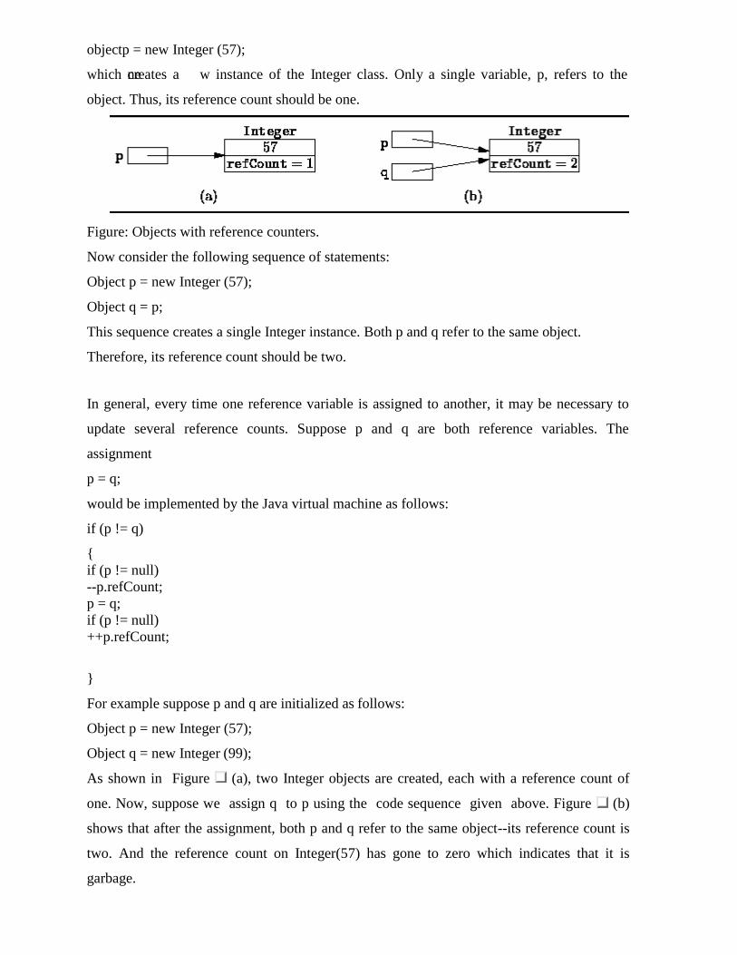
objectp = new Integer (57);
which ncreeates a w instance of the Integer class. Only a single variable, p, refers to the
object. Thus, its reference count should be one.
Figure: Objects with reference counters.
Now consider the following sequence of statements:
Object p = new Integer (57);
Object q = p;
This sequence creates a single Integer instance. Both p and q refer to the same object.
Therefore, its reference count should be two.
In general, every time one reference variable is assigned to another, it may be necessary to
update several reference counts. Suppose p and q are both reference variables. The
assignment
p = q;
would be implemented by the Java virtual machine as follows:
if (p != q)
{
if (p != null)
--p.refCount;
p = q;
if (p != null)
++p.refCount;
}
For example suppose p and q are initialized as follows:
Object p = new Integer (57);
Object q = new Integer (99);
As shown in Figure (a), two Integer objects are created, each with a reference count of
one. Now, suppose we assign q to p using the code sequence given above. Figure (b)
shows that after the assignment, both p and q refer to the same object--its reference count is
two. And the reference count on Integer(57) has gone to zero which indicates that it is
garbage.
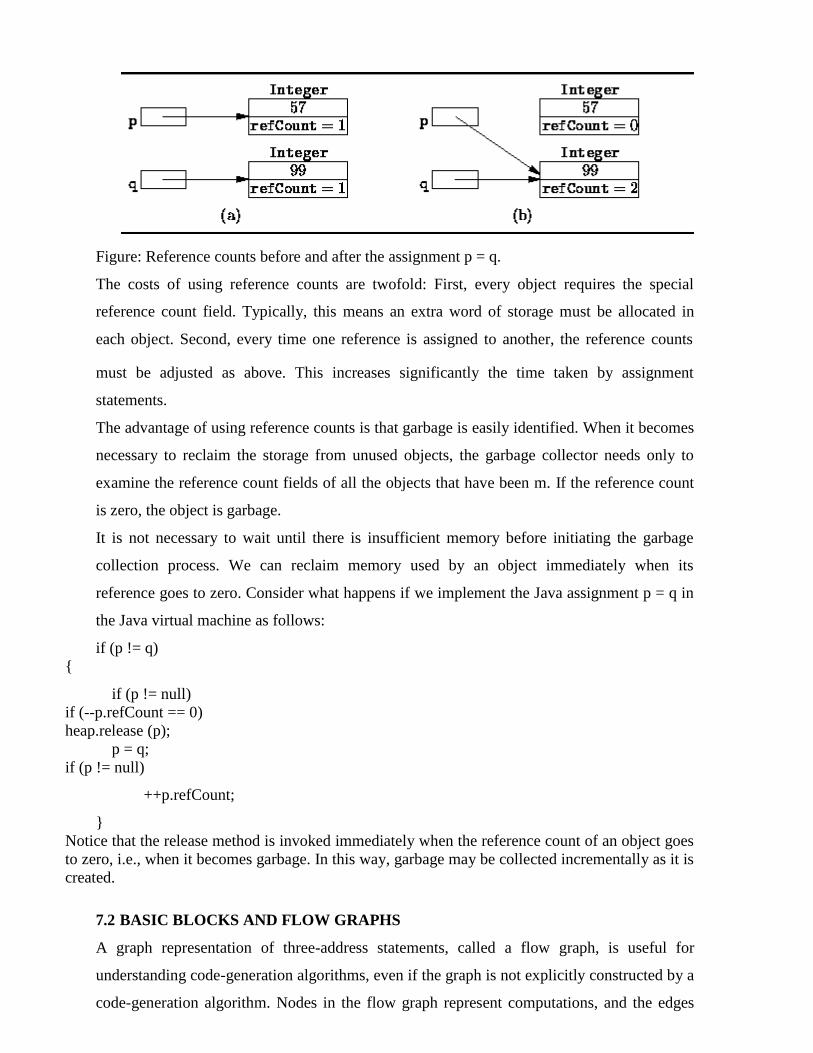
Figure: Reference counts before and after the assignment p = q.
The costs of using reference counts are twofold: First, every object requires the special
reference count field. Typically, this means an extra word of storage must be allocated in
each object. Second, every time one reference is assigned to another, the reference counts
must be adjusted as above. This increases significantly the time taken by assignment
statements.
The advantage of using reference counts is that garbage is easily identified. When it becomes
necessary to reclaim the storage from unused objects, the garbage collector needs only to
examine the reference count fields of all the objects that have been m. If the reference count
is zero, the object is garbage.
It is not necessary to wait until there is insufficient memory before initiating the garbage
collection process. We can reclaim memory used by an object immediately when its
reference goes to zero. Consider what happens if we implement the Java assignment p = q in
the Java virtual machine as follows:
if (p != q)
{
if (p != null)
if (--p.refCount == 0)
heap.release (p);
p = q;
if (p != null)
++p.refCount;
}
Notice that the release method is invoked immediately when the reference count of an object goes
to zero, i.e., when it becomes garbage. In this way, garbage may be collected incrementally as it is
created.
7.2 BASIC BLOCKS AND FLOW GRAPHS
A graph representation of three-address statements, called a flow graph, is useful for
understanding code-generation algorithms, even if the graph is not explicitly constructed by a
code-generation algorithm. Nodes in the flow graph represent computations, and the edges
represent the flow of control. Flow graph of a program can be used as a vehicle to collect
information about the intermediate program. Some register-assignment algorithms use flow
graphs to find the inner loops where a program is expected to spend most of its time.
BASIC BLOCKS
A basic block is a sequence of consecutive statements in which flow of control
enters at the beginning and leaves at the end without halt or possibility of branching except at
the end. The following sequence of three-address statements forms a basic block:
t1 := a*a
t2 := a*b
t3 := 2*t2
t4 := t1+t3
t5 := b*b
t6 := t4+t5
A three-address statement x := y+z is said to define x and to use y or z. A name in a basic
block is
vsaeida to lit a given point if its value is used after that point in the program,
perhaps in another basic block.
The following algorithm can be used to partition a sequence of three-address statements into
basic blocks.
Algorithm 1: Partition into basic blocks.
Input: A sequence of three-address statements.
Output: A list of basic blocks with each three-address statement in exactly one block.
Method:
1. We first determine the set of leaders, the first statements of basic
blocks. The rules we use are the following:
I) The first statement is a leader.
II) Any statement that is the target of a conditional or unconditional goto is a leader.
III) Any statement that immediately follows a goto or conditional goto statement
is a leader.
2. For each leader, its basic block consists of the leader and all statements up to but
not including the next leader or the end of the program.
Example 3: Consider the fragment of source code shown in fig. 7; it computes the dot
product of two vectors a and b of length 20. A list of three-address statements performing
this computation on our target machine is shown in fig. 8.
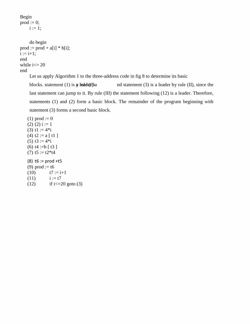
Begin
prod := 0;
i := 1;
do begin
prod := prod + a[i] * b[i];
i := i+1;
end
while i<= 20
end
Let us apply Algorithm 1 to the three-address code in fig 8 to determine its basic
blocks. statement (1) is ya lreualede(rI)ba nd statement (3) is a leader by rule (II), since the
last statement can jump to it. By rule (III) the statement following (12) is a leader. Therefore,
statements (1) and (2) form a basic block. The remainder of the program beginning with
statement (3) forms a second basic block.
(1) prod := 0
(2) (2) i := 1
(3) t1 := 4*i
(4) t2 := a [ t1 ]
(5) t3 := 4*i
(6) t4 :=b [ t3 ]
(7) t5 := t2*t4
(8) t6 := prod +t5 (9) prod := t6
(10) t7 := i+1
(11) i := t7
(12) if i<=20 goto (3)
UNIT –VI
Machine Independent Optimization. The principle sources of Optimization peep hole
Optimization, Introduction to Data flow Analysis
8.1 PRINCIPLE SOURCES OF OPTIMIZATION
A transformation of a program is called local if it can be performed by looking only at the
statements in a bas9ic block; otherwise, it is called global. Many transformations can be
performed at both the local and global levels. Local transformations are usually performed
first.
Function-Preserving Transformations There are a number of ways in which a compiler can
improve a program without changing the function it computes. Common sub expression
elimination, copy propagation, deadcode elimination, and constant folding are common
examples of such function-preserving transformations. The other transformations come up
primarily when global optimizations are performed. Frequently, a program will include
several calculations of the same value, such as an offset in an array. Some of these duplicate
calculations cannot be avoided by the programmer because they lie below the level of detail
accessible within the source language. For example, block B5 recalculates 4*i and 4*j.
Common Sub expressions An occurrence of an expression E is called a common sub
expression if E was previously computed, and the values of variables in E have not changed
since the previous computation. We can avoid re computing the expression if we can use the
previously computed value. For example, the assignments to t7 and t10 have the common sub
expressions 4*I and 4*j, respectively, on the right side in Fig. They have been eliminated in
Fig by using t6 instead of t7 and t8 instead of t10. This change is what would result if we
reconstructed the intermediate code from the dag for the basic block.
Example: the above Fig shows the result of eliminating both global and local common sub
expressions from blocks B5 and B6 in the flow graph of Fig. We first discuss the
transformation of B5 and then mention some subtleties involving arrays.
After local common sub expressions are eliminated B5 still evaluates 4*i and 4*j, as
Shown in the earlier fig. Both are common sub expressions; in particular, the three statements
t8:= 4*j; t9:= a[t[8]; a[t8]:=x in B5 can be replaced by t9:= a[t4]; a[t4:= x using t4 computed
in block B3. In Fig. observe that as control passes from the evaluation of 4*j in B3 to B5,
there is no change in j, so t4 can be used if 4*j is needed.
Another common sub expression comes to light in B5 after t4 replaces t8. The new
expression a[t4] corresponds to the value of a[j] at the source level. Not only does j retain its
value as control leaves b3 and then enters B5, but a[j], a value computed into a temporary t5,
does too because there are no assignments to elements of the array a in the interim. The
statement t9:= a[t4]; a[t6]:= t9 in B5 can therefore be replaced by
a[t6]:= t5 The expression in blocks B1 and B6 is not considered a common sub expression
although t1 can be used in both places. After control leaves B1 and before it reaches B6,it
can go through B5,where there are assignments to a. Hence, a[t1] may not have the same
value on reaching B6 as it did in leaving B1, and it is not safe to treat a[t1] as a common sub
expression.
Copy Propagation
Block B5 in Fig. can be further improved by eliminating x using two nsefwortmraations.
One concerns assignments of the form f:=g called copy statements, or copies for short. Had
we gone into more detail in Example 10.2, copies would have arisen much sooner, because
the algorithm for eliminating common sub expressions introduces them, as do several other
algorithms. For example, when the common sub expression in c:=d+e is eliminated in Fig.,
the algorithm uses a new variable t to hold the value of d+e. Since control may reach c:=d+e
either after the assignment to a or after the assignment to b, itncwoorruelcd be t to replace
c:=d+e by either c:=a or by c:=b. The idea behind the copy-propagation transformation is to use g
for f, wherever possible after the copy statement f:=g. For example, the assignment x:=t3 in block
B5 of Fig. is a copy. Copy propagation applied to B5 yields:
x:=t3
a[t2]:=t5
a[t4]:=t3
goto B2 Copies introduced during common subexpression elimination. This may not
appear to be an improvement, but as we shall see, it gives us the opportunity to eliminate
the assignment to x.
8.1 DEAD-CODE ELIMINATIONS
A variable is live at a point in a program if its value can be used subsequently; otherwise, it is
dead at that point. A related idea is dead or useless code, statements that compute values that
never get used. While the programmer is unlikely to introduce any dead code intentionally, it
may appear as the result of previous transformations. For example, we discussed the use of
debug that is set to true or false at various points in the program, and used in statements like
If (debug) print. By a data-flow analysis, it may be possible to deduce that each time the
program reaches this statement, the value of debug is lflaylse. Usua
particular statement Debug :=false
, it is rbecause the is one
That we can deduce to be the last assignment to debug prior to the test no matter what
sequence of ebrapnrocghreas th m actually takes. If copy propagation replaces debug by
false, then theprint statement is dead because it cannot be reached. We
can eliminate both the test and printing from the o9bject code. More
generally, deducing at compile time that the value of an expression is a
constant and using the constant instead is known as constant folding.
One advantage of copy propagation is that it often turns the copy
statement into dead code. For example, copy propagation followed by
dead-code elimination removes the assignment to x and transforms 1.1
into
a [t2 ] := t5
a [t4] := t3
goto B2
8.2 PEEPHOLE OPTIMIZATION
A statement-by-statement code-generations strategy often produce target
code that contains redundant instructions and suboptimal constructs .The
quality of such target code can be improved by applying “optimizing”
transformations to the target program.
A simple but effective technique for improving the target code is
peephole optimization, a method for trying to improving the performance
of the target program by examining a short sequence of target instructions
(called the peephole) and replacing these instructions by a shorter or
faster sequence, whenever possible.
The peephole is a small, moving window on the target program. The code in
the peephole need not contiguous, although some implementations do
require this. We shall give the following examples of program
transformations that are characteristic of peephole optimizations:
• Redundant-instructions elimination
• Flow-of-control optimizations
• Algebraic simplifications
• Use of machine idioms
REDUNTANT LOADS AND STORES
If we see the instructions sequence
(1) (1) MOV R0,a
(2) (2) MOV a,R0
-we can delete instructions (2) because whenever (2) is executed. (1) will
ensure that the value of a is already in register R0.If (2) had a label we
could not be sure that (1) was always executed immediately before (2)
and so we could not remove (2).
UNREACHABLE CODE
Another opportunity for peephole optimizations is the removal of unreachable
instructions. An unlabeled instruction immediately following an
unconditional jump may be removed. This operation can be repeated to
eliminate a sequence of instructions. For example, for debugging
purposes, a large program may have within it certain segments that are
executed only if a variable debug is 1.In C, the source code might look
like:
#define debug 0
….
If ( debug ) {
Print debugging information
}
In the intermediate representations the if-statement
may be translated as: If debug =1 goto L2
Goto L2
L1: print debugging information
L2: …………………………(a)
One obvious peephole optimization is to eliminate jumps over jumps
.Thus no matter what the value of debug; (a) can be replaced by:
If debug ≠1 goto L2
Print debugging information
L2: ……………………………(b)
As the argument of the statement of (b) evaluates to a constant true it can be replaced by
If debug ≠0 goto L2
Print debugging information
L2: ……………………………(c)
As the argument of the first statement of (c) evaluates to a constant true, it can
be replaced by goto L2. Then all the statement that print debugging aids are
manifestly unreachable and can be eliminated one at a time
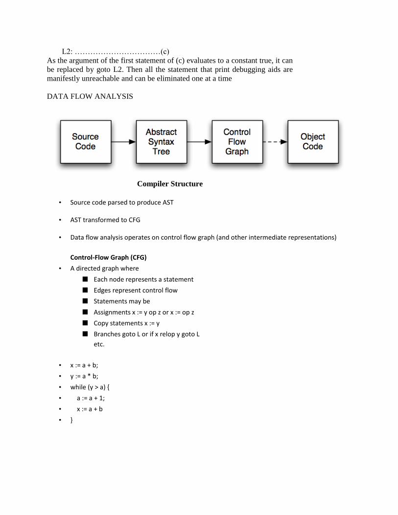
DATA FLOW ANALYSIS
Compiler Structure
• Source code parsed to produce AST
• AST transformed to CFG
• Data flow analysis operates on control flow graph (and other intermediate representations)
Control-Flow Graph (CFG)
• A directed graph where
■ Each node represents a statement
■ Edges represent control flow
■ Statements may be
■ Assignments x := y op z or x := op z
■ Copy statements x := y
■ Branches goto L or if x relop y goto L
etc.
• x := a + b;
• y := a * b;
• while (y > a) {
• a := a + 1;
• x := a + b
• }
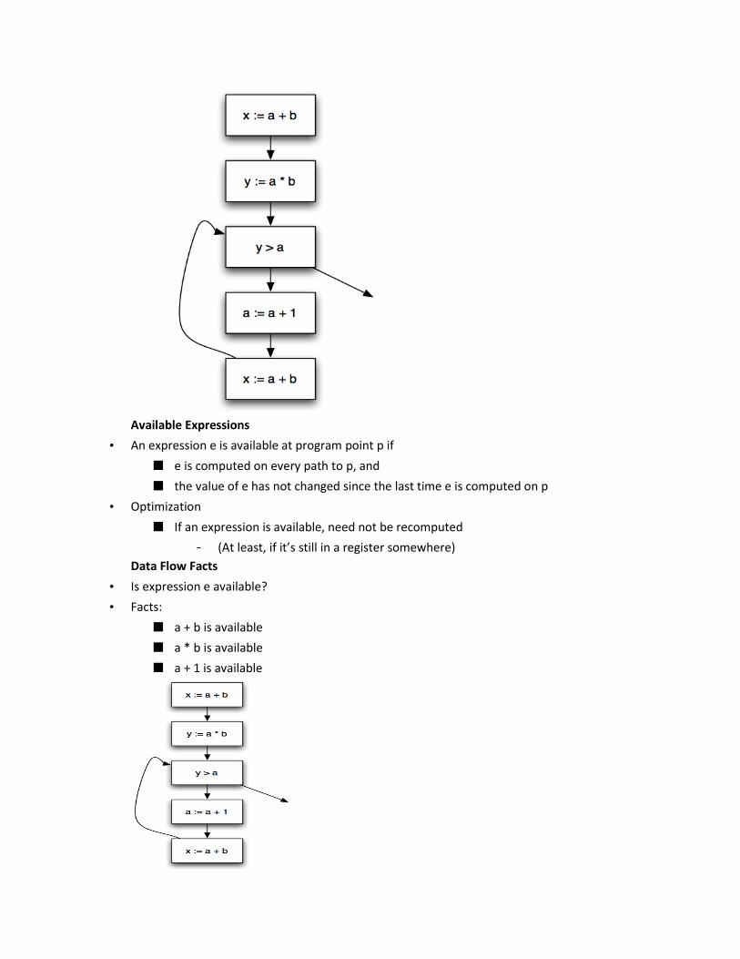
Available Expressions
• An expression e is available at program point p if
■ e is computed on every path to p, and
■ the value of e has not changed since the last time e is computed on p
• Optimization
■ If an expression is available, need not be recomputed
- (At least, if it’s still in a register somewhere)
Data Flow Facts
• Is expression e available?
• Facts:
■ a + b is available
■ a * b is available
■ a + 1 is available
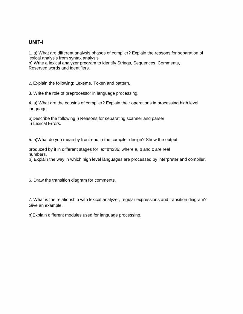
UNIT-I
1. a) What are different analysis phases of compiler? Explain the reasons for separation of lexical analysis from syntax analysis b) Write a lexical analyzer program to identify Strings, Sequences, Comments, Reserved words and identifiers.
2. Explain the following: Lexeme, Token and pattern.
3. Write the role of preprocessor in language processing.
4. a) What are the cousins of compiler? Explain their operations in processing high level
language.
b)Describe the following i) Reasons for separating scanner and parser ii) Lexical Errors.
5. a)What do you mean by front end in the compiler design? Show the output
produced by it in different stages for a:=b*c/36; where a, b and c are real numbers. b) Explain the way in which high level languages are processed by interpreter and compiler.
6. Draw the transition diagram for comments.
7. What is the relationship with lexical analyzer, regular expressions and transition diagram?
Give an example.
b)Explain different modules used for language processing.
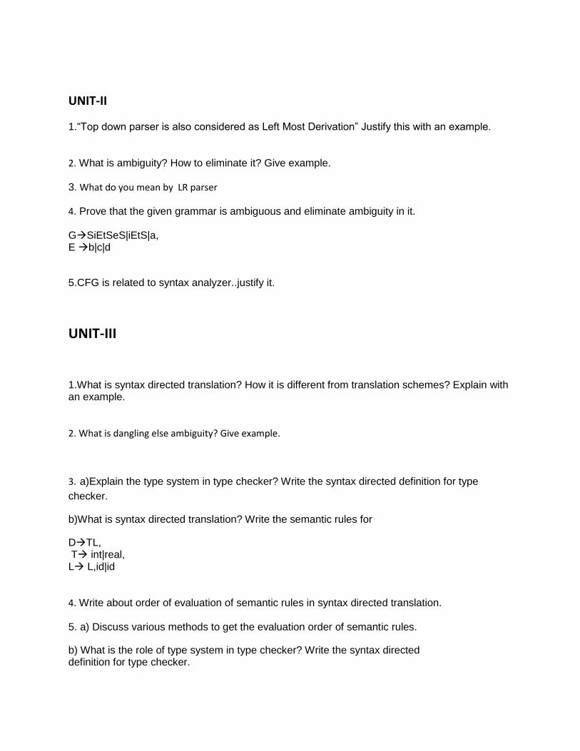
UNIT-II
1.“Top down parser is also considered as Left Most Derivation” Justify this with an example.
2. What is ambiguity? How to eliminate it? Give example.
3. What do you mean by LR parser
4. Prove that the given grammar is ambiguous and eliminate ambiguity in it.
G→SiEtSeS|iEtS|a, E →b|c|d
5.CFG is related to syntax analyzer..justify it.
UNIT-III
1.What is syntax directed translation? How it is different from translation schemes? Explain with an example.
2. What is dangling else ambiguity? Give example.
3. a)Explain the type system in type checker? Write the syntax directed definition for type
checker.
b)What is syntax directed translation? Write the semantic rules for
D→TL, T→ int|real, L→ L,id|id
4. Write about order of evaluation of semantic rules in syntax directed translation.
5. a) Discuss various methods to get the evaluation order of semantic rules.
b) What is the role of type system in type checker? Write the syntax directed definition for type checker.
UNIT IV
1) Explain various parameter passing mechanisms.
2) a)What is dependency graph? Construct dependency graph for the expression a-4+c using syntax directed definition of
E→TE1 E1→+TE1/-TE1/Є
T→(E)/id/num b) Differentiate inherited and synthesized attributes with an example.
3)Generate three address code for the given pseudo co de while(i<=100) { A=A/B*20; ++i; print(A value) }
4) a)What is syntax directed translation? How it is different from translation
schemes? Explain with an example. b)Translate the given expression into
Quadruples, triples and indirect triples
(a+b)*(c+d)+(a*b/c)*b+60.And list advantages and disadvantages.
5) a)Explain the type system in type checker? Write the syntax directed definition
for type checker.
b)What is syntax directed translation? Write the semantic rules for D→TL, T→int|real, L→L,id|id
UNIT V
1) Write various forms of object code generated in code generation phase.
2) a)What is runtime stack? Explain storage allocation strategies used for
recursive procedure calls.
b)Can we reuse the symbol table space? Explain through an example.
3) What is run time environment? Givethe structure.
4) a) What is scope of variable? Write about variousways to access non local
variables.
b)Generate target code from sequence of three address statements using simple code generator algorithm.
UNIT VI
1) For the code given in Q.1(d) generate the basic blocks and write the rules.
2) a) Differentiate various techniques used for machine independent and
dependent optimizations. b)Explain how code motion and frequency reduction used for loop optimizations? 3) Give the organization of optimizing compiler.
4) a) Write about the techniques in local and global transformations.
b)What do you mean by inter procedural optimization? Explain with examples.
5) How to schedule the instructions to produce optimized code? Explain.


