
U.S. Department of the InteriorU.S. Geological Survey
Scientific Investigations Report 2012–5120
National Water-Quality Assessment Program
Comparison of TOPMODEL Streamflow Simulations Using NEXRAD-Based and Measured Rainfall Data, McTier Creek Watershed, South Carolina
Daily
mea
n flo
w, i
n cu
bic
feet
per
sec
ond
140
130
120
110
100
90
80
70
60
50
40
30
20
10
0
2007 2008 2009J J A F M A MS O N D J J J A F M AS O M J J A S ON D J


Comparison of TOPMODEL Streamflow Simulations Using NEXRAD-Based and Measured Rainfall Data, McTier Creek Watershed, South Carolina
By Toby D. Feaster, Nancy E. Westcott, Robert J.M. Hudson, Paul A. Conrads, and Paul M. Bradley
National Water-Quality Assessment Program
Scientific Investigations Report 2012–5120
U.S. Department of the InteriorU.S. Geological Survey

U.S. Department of the InteriorKEN SALAZAR, Secretary
U.S. Geological SurveyMarcia K. McNutt, Director
U.S. Geological Survey, Reston, Virginia: 2012
For more information on the USGS—the Federal source for science about the Earth, its natural and living resources, natural hazards, and the environment, visit http://www.usgs.gov or call 1–888–ASK–USGS.
For an overview of USGS information products, including maps, imagery, and publications, visit http://www.usgs.gov/pubprod
To order this and other USGS information products, visit http://store.usgs.gov
Any use of trade, product, or firm names is for descriptive purposes only and does not imply endorsement by the U.S. Government.
Although this report is in the public domain, permission must be secured from the individual copyright owners to reproduce any copyrighted materials contained within this report.
Suggested citation:Feaster, T.D., Westcott, N.E., Hudson, R.J.M., Conrads, P..A., and Bradley P.M., 2012, Comparison of TOPMODEL streamflow simulations using NEXRAD-based and measured rainfall data, McTier Creek watershed, South Carolina: U.S. Geological Survey Scientific Investigations Report 2012–5120, 33 p.

iii
Foreword
The U.S. Geological Survey (USGS) is committed to providing the Nation with reliable scientific information that helps to enhance and protect the overall quality of life and that facilitates effec-tive management of water, biological, energy, and mineral resources (http://www.usgs.gov/). Information on the Nation’s water resources is critical to ensuring long-term availability of water that is safe for drinking and recreation and is suitable for industry, irrigation, and fish and wild-life. Population growth and increasing demands for water make the availability of that water, measured in terms of quantity and quality, even more essential to the long-term sustainability of our communities and ecosystems.
The USGS implemented the National Water-Quality Assessment (NAWQA) Program in 1991 to support national, regional, State, and local information needs and decisions related to water-quality management and policy (http://water.usgs.gov/nawqa). The NAWQA Program is designed to answer: What is the quality of our Nation’s streams and groundwater? How are conditions changing over time? How do natural features and human activities affect the quality of streams and groundwater, and where are those effects most pronounced? By combining information on water chemistry, physical characteristics, stream habitat, and aquatic life, the NAWQA Program aims to provide science-based insights for current and emerging water issues and priorities. From 1991 to 2001, the NAWQA Program completed interdisciplinary assessments and established a baseline understanding of water-quality conditions in 51 of the Nation’s river basins and aquifers, referred to as Study Units (http://water.usgs.gov/nawqa/studies/study_units.html).
National and regional assessments are ongoing in the second decade (2001–2012) of the NAWQA Program as 42 of the 51 Study Units are selectively reassessed. These assessments extend the findings in the Study Units by determining water-quality status and trends at sites that have been consistently monitored for more than a decade, and filling critical gaps in characterizing the quality of surface water and groundwater. For example, increased emphasis has been placed on assessing the quality of source water and finished water associated with many of the Nation’s largest community water systems. During the second decade, NAWQA is addressing five national priority topics that build an understanding of how natural features and human activities affect water quality, and establish links between sources of contaminants, the transport of those contaminants through the hydrologic system, and the potential effects of contaminants on humans and aquatic ecosystems. Included are studies on the fate of agricul-tural chemicals, effects of urbanization on stream ecosystems, bioaccumulation of mercury in stream ecosystems, effects of nutrient enrichment on aquatic ecosystems, and transport of contaminants to public-supply wells. In addition, national syntheses of information on pesti-cides, volatile organic compounds (VOCs), nutrients, trace elements, and aquatic ecology are continuing.
The USGS aims to disseminate credible, timely, and relevant science information to address practical and effective water-resource management and strategies that protect and restore water quality. We hope this NAWQA publication will provide you with insights and informa-tion to meet your needs, and will foster increased citizen awareness and involvement in the protection and restoration of our Nation’s waters.
iv
The USGS recognizes that a national assessment by a single program cannot address all water-resource issues of interest. External coordination at all levels is critical for cost-effective man-agement, regulation, and conservation of our Nation’s water resources. The NAWQA Program, therefore, depends on advice and information from other agencies—Federal, State, regional, interstate, Tribal, and local—as well as nongovernmental organizations, industry, academia, and other stakeholder groups. Your assistance and suggestions are greatly appreciated.
William H. Werkheiser USGS Associate Director for Water

v
Contents
Foreword ........................................................................................................................................................iiiAbstract ...........................................................................................................................................................1Introduction.....................................................................................................................................................2
Purpose and Scope ..............................................................................................................................2Previous Studies ...................................................................................................................................2Study Area..............................................................................................................................................3
Rainfall Data Comparisons ...........................................................................................................................5Measured Rainfall Data from NWS COOP Stations ........................................................................5Gridded Multisensor Precipitation Estimates ..................................................................................5Measured Rainfall and NEXRAD-Based Estimated Rainfall Comparisons Approach ..............7
Rainfall Comparison Statistics ...................................................................................................7Rainfall Comparison in McTier Creek Subwatersheds ...................................................................8
TOPMODEL Application ..............................................................................................................................13TOPMODEL Code Correction ............................................................................................................14
TOPMODEL Streamflow Simulations ........................................................................................................15Effects of TOPMODEL Code Correction ..........................................................................................16Streamflow Simulations Using NEXRAD-Based Rainfall Data ....................................................16
Monetta Streamflow .................................................................................................................17New Holland Streamflow .........................................................................................................17
Comparison of NWS COOP and NEXRAD-Based Rainfall Data Inputs for the Monetta and New Holland Watershed TOPMODEL Simulations ..................................................20
Recalibration of TOPMODEL Using NEXRAD-Based Rainfall Data ............................................21Monetta and New Holland Streamflow Simulations ...........................................................22
Streamflow Simulations in McTier Creek Subwatersheds ..........................................................23Summary and Conclusions .........................................................................................................................30References Cited..........................................................................................................................................31
Figures 1. Map showing location of the McTier Creek watershed, Aiken County,
South Carolina ...............................................................................................................................4 2. Map showing National Weather Service Cooperative meteorological stations
near the McTier Creek watershed, South Carolina, included in this investigation and NEXRAD-based grid locations ............................................................................................6
3. Graphs showing residuals of NEXRAD-based and measured rainfall at National Weather Service Cooperative meteorological station locations near the McTier Creek watershed, South Carolina ..............................................................................................9
4. Graphs showing NEXRAD-based and measured rainfall at National Weather Service Cooperative meteorological station locations near the McTier Creek watershed, South Carolina ........................................................................................................10
5. Map showing McTier Creek subwatersheds, Aiken County, South Carolina ...................11 6. Graph showing single-mass curves of NEXRAD-based daily rainfall for McTier
Creek subwatersheds MA01 to MA12 for June 13, 2007, to September 30, 2009 ............12

vi
7. Graph showing single-mass curves of cumulative rainfall at National Weather Service Cooperative meteorological stations near McTier Creek watershed for concurrent periods of record from June 13, 2007, to September 30, 2009 ........................12
8. Graph showing single-mass curves of cumulative NEXRAD-based rainfall at National Weather Service Cooperative meteorological station locations near the McTier Creek watershed for periods concurrent with the concurrent NWS COOP rainfall data from June 13, 2007, to September 30, 2009 ......................................................13
9. Diagram showing definition of selected water-source variables from TOPMODEL .......14 10. Graphs showing single-mass curves of simulated and observed daily mean flow
at McTier Creek watershed near Monetta and New Holland for June 13, 2007, to September 30, 2009 .....................................................................................................................18
11. Graphs showing TOPMODEL-C/C and TOPMODEL-C/N streamflow simulations in relation to observed streamflow for daily mean flows, flow-duration curves, and single-mass curves at McTier Creek near Monetta for June 13, 2007, to September 30, 2009 .....................................................................................................................18
12. Graphs showing TOPMODEL-C/C and TOPMODEL-C/N streamflow simulations in relation to observed streamflow for daily mean flows, flow-duration curves, and single-mass curves at McTier Creek near New Holland for June 13, 2007, to September 30, 2009 .....................................................................................................................20
13. Graph showing cumulative total daily measured rainfall for the McTier Creek watershed in relation to total daily NEXRAD-based rainfall for Monetta and New Holland ................................................................................................................................21
14. Graphs showing TOPMODEL-C/C and TOPMODEL-N/N streamflow simulations in relation to daily mean flows, flow-duration curves, and single-mass curves at McTier Creek near Monetta for June 13, 2007, to September 30, 2009 .............................24
15. Graphs showing TOPMODEL-C/C and TOPMODEL-N/N streamflow simulations in relation to observed streamflow for daily mean flows, flow-duration curves, and single-mass curves at McTier Creek near New Holland for June 13, 2007, to September 30, 2009 .....................................................................................................................24
16. Graphs showing TOPMODEL-C/C streamflow simulations of daily mean streamflow for June 13, 2007, to September 30, 2009, at McTier Creek near Monetta and the sum of the simulated daily mean streamflow for subwatersheds MA01 to MA06, and McTier Creek near New Holland and the sum of the simulated daily mean streamflow for subwatersheds MA01 to MA12 ................................................25
17. Graphs showing TOPMODEL-N/N streamflow simulations for June 13, 2007, to September 30, 2009, at McTier Creek near Monetta and the sum of simulated daily mean streamflow for subwatersheds MA01 to MA06, and McTier Creek near New Holland and the sum of simulated daily mean streamflow for subwatersheds MA01 to MA12 .............................................................................................................................25
18. Graphs showing TOPMODEL-C/C and TOPMODEL-N/N simulated daily mean streamflow at McTier Creek subwatersheds MA01 to MA12 for June 13, 2007, to September 30, 2009 .....................................................................................................................26
19. Map showing South Carolina precipitation, 1971–2000 .......................................................29

vii
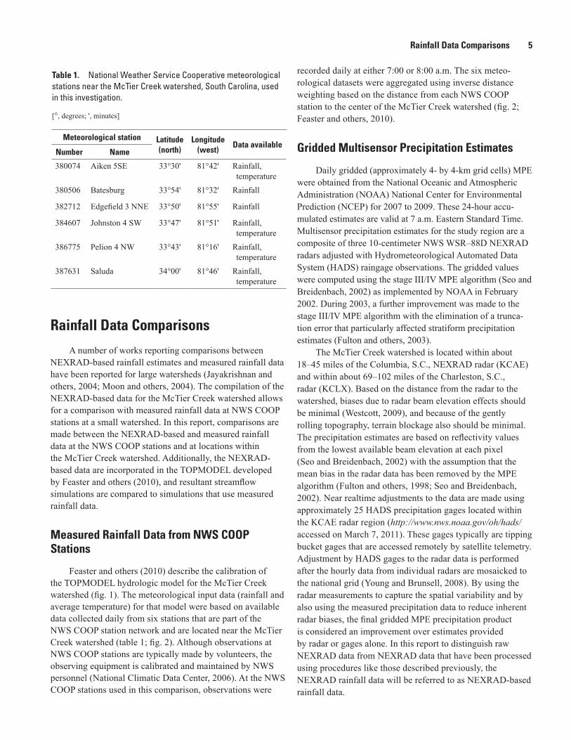
Tables 1. National Weather Service Cooperative meteorological stations near the McTier
Creek watershed, South Carolina, used in this investigation ................................................5 2. Comparison statistics with respect to days with non-zero rainfall for measured
and NEXRAD-based estimated daily rainfall for selected National Weather Service Cooperative stations near the McTier Creek watershed from June 13, 2007, to September 30, 2009 ........................................................................................................8
3. Parameter values used for the TOPMODEL calibration for McTier Creek near Monetta and for McTier Creek near New Holland for June 13, 2007, to September 30, 2009 .....................................................................................................................15
4. Station number and name, period of record used in the model simulations, and model simulation period reference name for the McTier Creek watershed, South Carolina .............................................................................................................................16
5. Goodness-of-fit statistics at McTier Creek near Monetta and McTier Creek near New Holland from Feaster and others (2010) and from the corrected TOPMODEL source code simulations for June 13, 2007, to September 30, 2009 ...................................17
6. Goodness-of-fit statistics for McTier Creek near Monetta for the June 13, 2007, to September 30, 2009 simulation .................................................................................................19
7. Goodness-of-fit statistics for McTier Creek near New Holland for the June 13, 2007, to September 30, 2009 simulation ...................................................................................19
8. Goodness-of-fit statistics for the McTier Creek near Monetta TOPMODEL simulations for June 13, 2007, to September 30, 2009 ...........................................................22
9. Goodness-of-fit statistics for the McTier Creek near New Holland TOPMODEL simulations for June 13, 2007, to September 30, 2009 ...........................................................23
10. McTier Creek subwatershed area and percent difference between TOPMODEL-C/C and TOPMODEL-N/N simulated total volume of daily mean streamflow ...................................................................................................................................28
11. Total NEXRAD-based rainfall by subwatershed and differences from total NEXRAD-based rainfall and total NWS COOP rainfall for McTier Creek near New Holland ................................................................................................................................28

viii
Conversion Factors and Abbreviations
SI to Inch/Pound
Multiply By To obtain
Length
centimeter (cm) 0.3937 inch (in.)meter (m) 3.281 foot (ft) kilometer (km) 0.6214 mile (mi)
Area
hectare (ha) 2.471 acresquare kilometer (km2) 247.1 acresquare kilometer (km2) 0.3861 square mile (mi2)
Volume
cubic meter (m3) 35.31 cubic foot (ft3)
Flow rate
meter per second (m/s) 3.281 foot per second (ft/s) cubic meter per day (m3/d) 35.31 cubic foot per day (ft3/d)
Hydraulic conductivity
meter per day (m/d) 3.281 foot per day (ft/d)
Hydraulic gradient
meter per kilometer (m/km) 5.27983 foot per mile (ft/mi)
Inch/Pound to SI
Multiply By To obtain
Length
inch (in.) 2.54 centimeter (cm)inch (in.) 25.4 millimeter (mm)foot (ft) 0.3048 meter (m)mile (mi) 1.609 kilometer (km)
Area
acre 0.004047 square kilometer (km2)square mile (mi2) 2.590 square kilometer (km2)
Volume
cubic foot (ft3) 0.02832 cubic meter (m3)
Flow rate
cubic foot per second (ft3/s) 0.02832 cubic meter per second (m3/s)cubic foot per second per square
mile [(ft3/s)/mi2]0.01093 cubic meter per second per
square kilometer [(m3/s)/km2]inch per hour (in/h) 0.0254 cubic meter per hour (m3/h)
Hydraulic conductivity
foot per day (ft/d) 0.3048 meter per day (m/d)

ix
Temperature in degrees Celsius (°C) may be converted to degrees Fahrenheit (°F) as follows:
°F=(1.8×°C)+32
Temperature in degrees Fahrenheit (°F) may be converted to degrees Celsius (°C) as follows:
°C=(°F–32)/1.8
Horizontal coordinate information is referenced to North American Datum of 1927 (NAD 27) or North American Datum of 1983 (NAD 83).
Vertical coordinate information is referenced to the North American Veritcal Datum of 1988 (NAVD 88) or National Geodetic Vertical Datum of 1929 (NGVD 29).
Elevation, as used in this report, refers to distance above the vertical datum.

Abbreviations
a.m. before midday
EE estimation efficiency
EST Eastern Standard Time
GBMM Grid-based mercury model
GIS Geographic information system
HADS Hydrometeorological Automated Data System
m scaling parameter
MA01–MA12 Model assessment points
MAE mean absolute error
Monetta Station 02172300, McTier Creek near Monetta, SC
MPE multisensor precipitation estimates
NEXRAD Next generation weather radar
New Holland Station 02172305, McTier Creek near New Holland, SC
NAWQA Natural Water-Quality Assessment Program
NOAA National Oceanic and Atmospheric Administration
NSE Nash-Sutcliffe coefficient of efficiency
NWS National Weather Service
NWS COOP National Weather Service cooperative station
PEST Parameter estimation program
r Pearson’s correlation coefficient
RMSD root mean square difference
RMSE root mean square error
SC South Carolina
SWAT Soil and Water Assessment Tool
TOPMODEL Topography-based hydrological model
TOPMODEL-C/C TOPMODEL calibration and simulations done using measured rainfall
TOPMODEL-C/N TOPMODEL calibration using measured rainfall and simulations using NEXRAD-based rainfall
TOPMODEL-N/N TOPMODEL calibration and simulations done using NEXRAD-based rainfall
USGS U.S. Geological Survey
WSR-88D Weather surveillance radar–1988 Doppler system

Comparison of TOPMODEL Streamflow Simulations Using NEXRAD-Based and Measured Rainfall Data, McTier Creek Watershed, South Carolina
By Toby D. Feaster1, Nancy E. Westcott2, Robert J.M. Hudson3, Paul A. Conrads1, and Paul M. Bradley1
1U.S. Geological Survey.
2Illinois State Water Survey, University of Illinois at Urbana-Champaign.
3University of Illinois at Urbana-Champaign.
AbstractRainfall is an important forcing function in most water-
shed models. As part of a previous investigation to assess interactions among hydrologic, geochemical, and ecological processes that affect fish-tissue mercury concentrations in the Edisto River Basin, the topography-based hydrological model (TOPMODEL) was applied in the McTier Creek watershed in Aiken County, South Carolina. Measured rainfall data from six National Weather Service (NWS) Cooperative (COOP) stations surrounding the McTier Creek watershed were used to calibrate the McTier Creek TOPMODEL. Since the 1990s, the next generation weather radar (NEXRAD) has provided rainfall estimates at a finer spatial and temporal resolution than the NWS COOP network. For this investigation, NEXRAD-based rainfall data were generated at the NWS COOP stations and compared with measured rainfall data for the period June 13, 2007, to September 30, 2009. Likewise, these NEXRAD-based rainfall data were used with TOPMODEL to simulate streamflow in the McTier Creek watershed and then compared with the simulations made using measured rainfall data. NEXRAD-based rainfall data for non-zero rainfall days were lower than measured rainfall data at all six NWS COOP locations. The total number of concurrent days for which both measured and NEXRAD-based data were available at the COOP stations ranged from 501 to 833, the number of non-zero days ranged from 139 to 209, and the total difference in rainfall ranged from –1.3 to –21.6 inches.
With the calibrated TOPMODEL, simulations using NEXRAD-based rainfall data and those using measured rainfall data produce similar results with respect to matching the timing and shape of the hydrographs. Comparison of the bias, which is the mean of the residuals between observed and simulated streamflow, however, reveals that simulations using NEXRAD-based rainfall tended to underpredict streamflow overall. Given that the total NEXRAD-based rainfall data for
the simulation period is lower than the total measured rainfall at the NWS COOP locations, this bias would be expected. Therefore, to better assess the use of NEXRAD-based rainfall estimates as compared to NWS COOP rainfall data on the hydrologic simulations, TOPMODEL was recalibrated and updated simulations were made using the NEXRAD-based rainfall data. Comparisons of observed and simulated stream-flow show that the TOPMODEL results using measured rainfall data and NEXRAD-based rainfall are comparable. Nonetheless, TOPMODEL simulations using NEXRAD-based rainfall still tended to underpredict total streamflow volume, although the magnitude of differences were similar to the simulations using measured rainfall.
The McTier Creek watershed was subdivided into 12 subwatersheds and NEXRAD-based rainfall data were generated for each subwatershed. Simulations of streamflow were generated for each subwatershed using NEXRAD-based rainfall and compared with subwatershed simulations using measured rainfall data, which unlike the NEXRAD-based rainfall were the same data for all subwatersheds (derived from a weighted average of the six NWS COOP stations surrounding the basin). For the two simulations, subwater-shed streamflow were summed and compared to streamflow simulations at two U.S. Geological Survey streamgages. The percentage differences at the gage near Monetta, South Caro-lina, were the same for simulations using measured rainfall data and NEXRAD-based rainfall. At the gage near New Holland, South Carolina, the percentage differences using the NEXRAD-based rainfall were twice as much as those using the measured rainfall. Single-mass curve comparisons showed an increase in the total volume of rainfall from north to south. Similar comparisons of the measured rainfall at the NWS COOP stations showed similar percentage differences, but the NEXRAD-based rainfall variations occurred over a much smaller distance than the measured rainfall. Nonethe-less, it was concluded that in some cases, using NEXRAD-based rainfall data in TOPMODEL streamflow simulations may provide an effective alternative to using measured rainfall data. For this investigation, however, TOPMODEL streamflow simulations using NEXRAD-based rainfall data

2 Comparison of TOPMODEL Streamflow Simulations Using NEXRAD-Based and Measured Rainfall Data
for both calibration and simulations did not show significant improvements with respect to matching observed streamflow over simulations generated using measured rainfall data.
IntroductionRainfall is an essential forcing function for hydrologic
models. Traditionally, rainfall data collected at specific gages, often on a 24-hour basis, have been used for hydrologic model inputs (Beven, 2001). To help compensate for the temporal and spatial variability that naturally occurs in rainfall, numerous techniques are available for integrating or weighting data from various gages in and (or) around a modeled water-shed (Shepard, 1968; Maidment, 1993; Bedient and others, 2008). In the fall of 1990, the first weather surveillance radar-1988 Doppler (WSR–88D) system was installed near Okla-homa City, Oklahoma (Crum and Alberty, 1993). Since that time, the next generation weather radar (NEXRAD) network of WSR–88D units has provided rainfall estimates that have finer spatial and temporal resolution than the National Weather Service (NWS) Cooperative (COOP) stations. The WSR–88D precipitation estimation consists of several processing stages (Hardegree and others, 2008). Stage I occurs at the individual radar site producing spatial rainfall estimates for a single radar domain. Stages II and III involve, respectively, multisensory bias adjustment and creation of a multiradar mosaic of precipi-tation estimates for areas with overlapping radar coverage. In Stage IV, the multisensor estimates undergo an additional process that involves the mosaicking of the estimates from all the NWS River Forecast Centers (Habib and others, 2009). Although the technology continues to improve, comparisons have shown that uncertainties associated with the NEXRAD-based data should be considered (National Climatic Data Center, 1996; Seo and Breidenbach, 2002; Jayakrishnan and others, 2004; Moon and others, 2004; Hardegree and others, 2008; and Young and Brunsell, 2008).
Two hydrologic models were developed for the McTier Creek watershed in Aiken County, South Carolina (Feaster and others, 2010) to advance understanding of the fate and transport of mercury in stream ecosystems and to expand the understanding of hydrologic, geochemical, and ecological processes within the Edisto River Basin that affect fish-tissue mercury concentrations (Bradley and others, 2011). The two models are the topography-based hydrological model (TOPMODEL) (Kennen and others, 2008) and the grid-based mercury model (GBMM) (Dai and others, 2005; Tetra Tech, 2006). The rainfall data used for the models were obtained from six National Weather Service (NWS) Cooperative (COOP) stations. In the current follow-up assessment of the water balance for the McTier Creek watershed, NEXRAD-based data were compiled for the 6 NWS COOP stations and for 12 subbasins in the McTier Creek watershed. Hereafter, the NWS COOP measured rainfall data will be referred to as measured rainfall. This research effort is part of the U.S. Geological Survey (USGS) National Water-Quality Assessment (NAWQA) Program.
Purpose and Scope
The purpose of this report is to document the results of a study to compare measured rainfall data at NWS COOP stations with estimated NEXRAD-based rainfall data for a specific small watershed. The report also documents the evalu-ation of using different rainfall data on simulated streamflow using TOPMODEL as described by Feaster and others (2010). The evaluation of simulated streamflow includes documenta-tion of the recalibration of TOPMODEL using the NEXRAD-based rainfall inputs. The scope of the report includes the McTier Creek watershed located in Aiken County, S.C., and areas gaged by six NWS COOP stations surrounding the McTier Creek watershed located in Saluda, Lexington, and Edgefield Counties, S.C.
An important part of the USGS mission is to provide scientific information for the effective water-resources management of the Nation (U.S. Geological Survey, 2007). To assess the quantity and quality of the Nation’s surface water, the USGS collects hydrologic and water-quality data from rivers, lakes, and estuaries by using standardized methods and maintains the data in a national database. These data are analyzed and used for hydrologic simulation models to enhance the understanding of the dynamics of hydrologic systems. The techniques presented in this report demonstrate selected approaches for comparing hydrologic datasets and for evalu-ating the effect on simulated output from hydrologic models.
Previous Studies
Numerous investigations have compared measured rainfall data, which occurred over areas much larger than the current investigation, to estimates obtained from the NWS radar system. The National Climatic Data Center (1996) compared NEXRAD-estimated storm-total precipitation with measured precipitation for five events: Missouri-Kansas April 1994, Southeast Texas October 1994, Florida November 1994, Louisiana-Mississippi-Alabama May 1995, and South Carolina-North Carolina-Georgia August 1995. The five events were chosen on the basis of both their extensive and damaging nature and the availability of one or more NEXRAD sites with suitable areal coverage. For 80 percent of the 220 raingage stations included in the National Climatic Data Center study (1996), the NEXRAD estimates were too low, sometimes by a factor of 2 to 3. As a result of the study, precipitation processing parameters were changed at some sites in an attempt to improve the rainfall estimates.
Smith and others (1996) compared about 1 year of WSR–88D hourly precipitation estimates with raingage data from the Southern Plains of Texas and Oklahoma. The study focused on systematic biases that affect the radar estimates. Numerous issues were discussed with respect to biases relating to distance from the radar. Within a 40-kilometer (km) range, bias due to reflectivity observations at high elevation angles caused significant underestimation of rainfall. Beyond 100 km,

Introduction 3
considerable underestimation of precipitation occurred. It was noted that spatial analysis of heavy rainfall showed advantages of radar over the raingage network.
Mizzell (1999) presents findings from a comparison of WSR–88D rainfall estimates with measured rainfall data in Lexington County, S.C., which forms the northern border of Aiken County, S.C., the county in which the McTier Creek watershed being analyzed in the current investigation resides. Mizzell (1999) compared radar estimates from the NWS WSR–88D radar located at the Columbia Airport in Lexington, S.C., with measured rainfall at 72 raingages. The study focused on seven precipitation events, which occurred between September 1997 and September 1998, that covered a variety of storm types, such as convective storms, tropical systems, and stratiform events. Results showed that radar estimates consistently underestimated measured rainfall, regardless of the storm type.
Jayakrishnan and others (2004) compared measured rainfall with WSR–88D Stage III precipitation data over the Texas-Gulf basin at 545 raingages for the period 1995 to 1999. The results showed that underestimation bias occurred at the majority of the stations analyzed. The study found that, in general, the radar estimates showed improvement over the years of the study, which was consistent with the ongoing improvement in developments of processing algorithms for the radar estimates. The paper also provides a thorough discussion of previous studies that readers are encouraged to review for additional information.
Young and Brunsell (2008) compared NEXRAD and multisensor precipitation estimates (MPE) in the Missouri River Basin with NWS COOP rainfall data. The raingage network was independent of the data used to develop the NEXRAD products and, therefore, provided an independent assessment of the NEXRAD data, which covered the period 1998 to 2004. The overall bias for NEXRAD data was –39 percent for the cold season and –32 percent for the warm season. As was noted by Jayakrishnan and others (2004), the NEXRAD estimates showed improvement over the period of the study with the warm season bias decreasing from –44 percent in 1998 to –15 percent in 2004.
In addition to numerous studies comparing NEXRAD-based rainfall data with measured rainfall data, many studies have compared the differences between simulations of streamflow using raingage data and NEXRAD-based data as rainfall inputs to hydrologic models. Moon and others (2004) performed such a comparison using the Soil and Water Assessment Tool (SWAT) in the Trinity River Basin of Texas. Regression analysis was used to compare the raingage and NEXRAD data at six raingages used in the investigation. The coefficient of determination (R2) for the six gages ranged from 0.43 to 0.80 with the Nash-Sutcliffe coefficient of efficiency (NSE) ranging from 0.28 to 0.77. For comparisons of simulated streamflow using NEXRAD-based rainfall with streamflow simulations using measured rainfall data, the NSE ranged from 0.57 to 0.82 and 0.48 to 0.78, respectively. In general, SWAT-NEXRAD simulations overpredicted high-flow
events and underpredicted low-flow events. Nonetheless, the authors concluded that NEXRAD-based rainfall data were a good alternative to measured rainfall data.
Sexton and others (2010) compared results from using measured raingage data and various NEXRAD MPE precipi-tation datasets (non-corrected, bias corrected, and inverse distance weighted corrected) on SWAT model simulations in a small Northeastern watershed. The SWAT was calibrated using each source of precipitation data, and streamflow simu-lations were compared to measured streamflow data. The NSE for calibration and validation simulations using measured rainfall ranged from 0.42 to 0.73, and R2 values ranged from 0.42 to 0.75. For the simulations using NEXRAD rainfall data, NSE values ranged from 0.46 to 0.76, and R2 ranged from 0.47 to 0.76. The study showed that for watersheds with no raingages in the watershed, the proximity of raingages outside the watershed and the direction of storm patterns can be important. Given these conditions, the conclusion was that NEXRAD data can be a good alternative to measured rainfall data.
Study Area
McTier Creek is a small headwater stream located in the Edisto River Basin and is a tributary to the South Fork Edisto River (fig. 1). The entire McTier Creek watershed encompasses about 38 square miles (mi2), is designated by the 12-digit hydrologic unit code 030502040102, and lies completely in the County of Aiken, S.C. (Eidson and others, 2005). The study area encompasses about 31 mi2.
McTier Creek lies within the inland part of the Coastal Plain Physiographic Province known as the Sand Hills (Griffith and others, 2002; fig. 1). Some studies integrate the Sand Hills within a broader area referred to as the inner or upper Coastal Plain (Bloxham, 1976). The headwaters of the McTier Creek watershed are located near the Fall Line (fig. 1), which is the name given to the boundary between the Piedmont and Coastal Plain Physiographic Provinces. In general, this boundary is characterized by a series of rapids or falls where the streams cascade off the more resistant rocks of the Piedmont into the deeper valleys worn into the softer sandy sediments of the Coastal Plain (Cooke, 1936). Commonly, the headwaters of watersheds located just below the Fall Line transition from characteristics similar to Pied-mont streams to characteristics of the Coastal Plain down-stream. In the upper part of the McTier Creek watershed, the channel is characterized by rock outcrops, a characteristic of many Piedmont streams.
As typically defined, precipitation occurs in a variety of forms such as hail, rain, freezing rain, sleet, or snow. In the South Carolina Coastal Plain environment, the majority of precipitation is in the form of rain. During the period covered in this report, no major frozen precipitation events were noted. Thus, in this report, precipitation is often being referred to simply as rainfall.

4 Comparison of TOPMODEL Streamflow Simulations Using NEXRAD-Based and Measured Rainfall Data
Figure 1. Location of the McTier Creek watershed, Aiken County, South Carolina (modfied from Feaster and others, 2010).
02172305
81°36' 81°32'
33°52'
33°48'
33°44'
Watershedboundary
Fall Line
SOUTH
ATLANTICOCEAN
GEORGIA
McTier Creekwatershed
Blue Ridge
Piedmont
Lower
Coastal Plain
Sand Hills
FallLine
Upper
Coastal Plain
NORTH CAROLINA
CAROLINA
Base from National Hydrography Dataset and digital line graphs, 1:100,000ESRI data and maps, 2006Albers equal area projection; central meridian-96 00 00; datum NAD 83
South
McTier
Gully
Creek
Creek
Fork EdistoRiver
20
SALUDA
AIKEN
U.S. Geological Survey streamgagingstation and number
EXPLANATION02172305
02172300
0 1 2 KILOMETERS0.5
0 1 2 MILES0.5
Rainfall Data Comparisons 5
Rainfall Data Comparisons
A number of works reporting comparisons between NEXRAD-based rainfall estimates and measured rainfall data have been reported for large watersheds (Jayakrishnan and others, 2004; Moon and others, 2004). The compilation of the NEXRAD-based data for the McTier Creek watershed allows for a comparison with measured rainfall data at NWS COOP stations at a small watershed. In this report, comparisons are made between the NEXRAD-based and measured rainfall data at the NWS COOP stations and at locations within the McTier Creek watershed. Additionally, the NEXRAD-based data are incorporated in the TOPMODEL developed by Feaster and others (2010), and resultant streamflow simulations are compared to simulations that use measured rainfall data.
Measured Rainfall Data from NWS COOP Stations
Feaster and others (2010) describe the calibration of the TOPMODEL hydrologic model for the McTier Creek watershed (fig. 1). The meteorological input data (rainfall and average temperature) for that model were based on available data collected daily from six stations that are part of the NWS COOP station network and are located near the McTier Creek watershed (table 1; fig. 2). Although observations at NWS COOP stations are typically made by volunteers, the observing equipment is calibrated and maintained by NWS personnel (National Climatic Data Center, 2006). At the NWS COOP stations used in this comparison, observations were
recorded daily at either 7:00 or 8:00 a.m. The six meteo-rological datasets were aggregated using inverse distance weighting based on the distance from each NWS COOP station to the center of the McTier Creek watershed (fig. 2; Feaster and others, 2010).
Gridded Multisensor Precipitation Estimates
Daily gridded (approximately 4- by 4-km grid cells) MPE were obtained from the National Oceanic and Atmospheric Administration (NOAA) National Center for Environmental Prediction (NCEP) for 2007 to 2009. These 24-hour accu-mulated estimates are valid at 7 a.m. Eastern Standard Time. Multisensor precipitation estimates for the study region are a composite of three 10-centimeter NWS WSR–88D NEXRAD radars adjusted with Hydrometeorological Automated Data System (HADS) raingage observations. The gridded values were computed using the stage III/IV MPE algorithm (Seo and Breidenbach, 2002) as implemented by NOAA in February 2002. During 2003, a further improvement was made to the stage III/IV MPE algorithm with the elimination of a trunca-tion error that particularly affected stratiform precipitation estimates (Fulton and others, 2003).
The McTier Creek watershed is located within about 18–45 miles of the Columbia, S.C., NEXRAD radar (KCAE) and within about 69–102 miles of the Charleston, S.C., radar (KCLX). Based on the distance from the radar to the watershed, biases due to radar beam elevation effects should be minimal (Westcott, 2009), and because of the gently rolling topography, terrain blockage also should be minimal. The precipitation estimates are based on reflectivity values from the lowest available beam elevation at each pixel (Seo and Breidenbach, 2002) with the assumption that the mean bias in the radar data has been removed by the MPE algorithm (Fulton and others, 1998; Seo and Breidenbach, 2002). Near realtime adjustments to the data are made using approximately 25 HADS precipitation gages located within the KCAE radar region (http://www.nws.noaa.gov/oh/hads/ accessed on March 7, 2011). These gages typically are tipping bucket gages that are accessed remotely by satellite telemetry. Adjustment by HADS gages to the radar data is performed after the hourly data from individual radars are mosaicked to the national grid (Young and Brunsell, 2008). By using the radar measurements to capture the spatial variability and by also using the measured precipitation data to reduce inherent radar biases, the final gridded MPE precipitation product is considered an improvement over estimates provided by radar or gages alone. In this report to distinguish raw NEXRAD data from NEXRAD data that have been processed using procedures like those described previously, the NEXRAD rainfall data will be referred to as NEXRAD-based rainfall data.
Table 1. National Weather Service Cooperative meteorological stations near the McTier Creek watershed, South Carolina, used in this investigation.
[°, degrees; ', minutes]
Meteorological station Latitude (north)
Longitude (west)
Data availableNumber Name
380074 Aiken 5SE 33°30' 81°42' Rainfall, temperature
380506 Batesburg 33°54' 81°32' Rainfall
382712 Edgefield 3 NNE 33°50' 81°55' Rainfall
384607 Johnston 4 SW 33°47' 81°51' Rainfall, temperature
386775 Pelion 4 NW 33°43' 81°16' Rainfall, temperature
387631 Saluda 34°00' 81°46' Rainfall, temperature

6 Comparison of TOPMODEL Streamflow Simulations Using NEXRAD-Based and Measured Rainfall Data
Figure 2. National Weather Service Cooperative (NWS COOP) meteorological stations near the McTier Creek watershed, South Carolina, included in this investigation and NEXRAD-based grid locations.
Saluda
Batesburg
Aiken 5SE
Pelion 4NW
Johnston 4SW
Edgefield 3NNE
Watershedboundary
02172305
20.3
6
19.17
18.85
18.2214.68
9.02
1.9
81°15'81°30'81°45'
34°
33°45'
33°30'
SALUDA
AIKEN
LEXINGTON
EDGEFIELD
RICHLAND
ORANGEBURG
NEWBERRY
Base from ESRI® Data & Maps, 2010Albers Equal-Area Conic projectionStandard parallels 29 30 N and 45 30 NCentral meridian -96 00 00
BARNWELL
0
6 12 KILOMETERS30
6 12 MILES3
EXPLANATIONNEXRAD grid
U.S. Geological Survey gagingstation and number
National Weather Service cooperative stations
Precipitation and temperature collection
Precipitation collection
Note: distances on map are in miles
02172305

Rainfall Data Comparisons 7
Measured Rainfall and NEXRAD-Based Estimated Rainfall Comparisons Approach
In recent years, progress has been made in the collection and processing of NEXRAD-based data to help address some of the biases associated with those data (Nelson and others, 2010). Measured rainfall at gaging stations also are not completely error free. Factors such as poor gage location or changing conditions near the gage, wind-induced issues, and human error are just some of the areas where uncertainty could be introduced into the measured data (Young and Brunsell, 2008). In addition, there is substantial disparity in the scale of the NEXRAD-based data and the measured rainfall data. The typical NWS COOP raingage has an 8-inch opening. The NEXRAD-based estimates are from an approximately 4- by 4-km grid in which the NWS COOP gage resides. However, because both estimates are 24-hour values and are spatially colocated, it is expected that the precipitation accumulations measured by both approaches are similar. Regardless, if similar patterns are detected at a number of locations, useful insights can be obtained.
In this study, both graphical and analytical methods were used to compare the measured rainfall and NEXRAD-based estimated rainfall at the NWS COOP station locations listed in table 1 for June 13, 2007, to September 30, 2009. This was the same period for which TOPMODEL simulations were gener-ated at USGS gaging stations 02172300, McTier Creek near Monetta, SC, and 02172305, McTier Creek near New Holland, SC, as documented in Feaster and others (2010). Hereafter, USGS gaging stations 02172300 and 02172305 will be referred to as Monetta and New Holland, respectively (fig. 1). The measured data represent the daily accumulation of precipita-tion at the NWS COOP station locations, and the NEXRAD-based data represent the estimated data from the grid cells that contain the NWS COOP station locations. Descriptive statistics were computed using only days when the rainfall was not zero for either the measured or the NEXRAD-based data (conditional statistics) (Jayakrishnan and others, 2004).
Using the conditional data (days for which non-zero accumulations were reported for both the NEXRAD-based and measured data), the measured 24-hour rainfall at the NWS COOP stations and the concurrent NEXRAD-based estimates were compared using the following descriptive statistics: (1) total difference in rainfall, (2) estimation bias, (3) estima-tion efficiency, and (4) root mean square difference. The total difference in rainfall is simply the difference between the total of the NEXRAD-based estimates minus the total measured rainfall from the NWS COOP station for the assessment period.
Total difference in rainfall (inches) = NEXRAD-based total – measured total
(1)
Estimation bias is the normalized difference between the total NEXRAD-based estimates and total measured rainfall for the comparison period and, therefore, is a comparison of total
rainfall volume. A negative estimation bias indicates that the total NEXRAD-based rainfall is less than the total measured rainfall.
Estimation bias (percent) = 100 × (NEXRAD-based total –
measured total)/measured total (2)
Estimation efficiency (EE) is the same as the NSE (Nash and Sutcliffe, 1970), which is widely used to assess agree-ment between measured and modeled timeseries data such as streamflow (Feaster and others, 2010). For the NEXRAD-based and measured rainfall comparisons, the estimation efficiency is computed as
EER W
R R
i ii
n
i m
i
n= −−
−
=
=
∑
∑1
2
1
2
1
( )
( ),
(3)
where n is the number of days of comparison; Ri is the measured rainfall for day i; Wi is the NEXRAD-based rainfall for the day i;
and Rm is the mean measured rainfall for all days.The root mean squared difference (RMSD) between the measured rainfall and the NEXRAD-based estimated rainfall is computed as
RMSD
R Wni i=−∑ ( )2
,
(4)
where the variables are as previously defined. A lower RMSD indicates better agreement between
the data being compared; however, the RMSD is sensitive to outliers because the differences in the data are squared (Janssen and Heuberger, 1993).
Rainfall Comparison StatisticsComparison statistics for the measured data at the NWS
COOP stations and the NEXRAD-based data estimated for the grid locations containing the NWS COOP stations indicate that the NEXRAD-based estimates were less than the measured rainfall at every location (table 2). The total difference in rain-fall ranged from –1.3 inches at Batesburg to –21.6 inches at Pelion 4 NW. The estimation bias ranged from –1.6 percent at Batesburg to –24.1 percent at Edgefield 3 NNE. Jayakrishnan and others (2004) reported similar estimation bias in an investigation over a much larger area in the Texas-Gulf Basin. For that investigation, estimation bias indicated underestima-tion of rainfall at 88 percent of the COOP locations. Another study, which included 72 raingages in nearby Lexington

8 Comparison of TOPMODEL Streamflow Simulations Using NEXRAD-Based and Measured Rainfall Data
County, S.C., and compared seven rainfall events covering a variety of storm types, showed that NEXRAD-based estimates consistently underestimated measured rainfall regardless of the storm type (Mizzell, 1999).
Residuals, which were computed for each day by subtracting the measured rainfall value from the NEXRAD-based estimated rainfall value, do not appear to indicate a geographical pattern at the six NWS COOP station locations (figs. 3 and 4). For example, the Saluda, Edgefield 3 NNE, and Johnston 4 SW locations are all in a quadrant northwest of the McTier Creek watershed (fig. 2). Johnston 4 SW and Saluda have the highest estimation efficiency and lowest RMSD of the six locations, whereas Edgefield 3 NNE has the lowest estimation efficiency and highest RMSD. It is interesting that Batesburg and Saluda, the two locations farthest north of the McTier Creek watershed, have the lowest estimation bias; however, Edgefield 3 NNE and Pelion 4 NW, which are located the farthest west and east of the watershed, have similar estimation bias at –24.1 and –21.3 percent, respectively, the highest of all the stations.
Residuals at each location are fairly consistent throughout the comparison period with a few exceptions (fig. 3). For the Edgefield 3 NNE location, residual scatter tended to increase slightly during the later part of the comparison period. At the Johnston 4 SW location, an increase in the negative residuals is noted in the later part of the record. The residuals for the Pelion 4 NW location are the most consistent over the entire comparison period.
In addition to the residuals, scatter plots of the data were generated, including a line of equal value to help distinguish estimation bias. As noted earlier, the Edgefield 3 NNE and Pelion 4 NW locations had the largest estimation biases (fig. 4). The plots indicate an underestimation bias by NEXRAD-based estimates during large rain events at all locations and is especially evident at the Edgefield 3 NNE location. In addition, the plots show that the majority of rainfall events for the comparison period were less than 1 inch.
Thus, calibration of the NEXRAD-based system is likely to be heavily weighted toward “normal” rainfall events, creating greater uncertainty in NEXRAD-based estimates for the infrequent, larger rainfall events. This situation is consistent with Westcott and others (2008) who found that larger events were underestimated by the NEXRAD-based estimates in the central Midwest.
Rainfall Comparison in McTier Creek Subwatersheds
One of the potential benefits of using NEXRAD-based rainfall data is the ability to generate a unique set of input rain-fall data for subsections of a watershed under consideration. In Feaster and others (2010), the McTier Creek watershed was subdivided into 12 subwatersheds, and streamflow was simulated for each subwatershed for the period June 13, 2007, to September 30, 2009 (fig. 5). To derive NEXRAD-based daily precipitation for the subwatersheds, the Thiessen polygon algorithm was applied in ArcGIS to the center points of each NEXRAD-based grid cell, and the resultant polygons were mapped onto the 12 subwatersheds within the McTier Creek Basin above New Holland. Single-mass curves of the NEXRAD-based rainfall data were generated for the subwa-tersheds (fig. 6). The plot shows that the NEXRAD-based rainfall was similar for all subwatersheds through the summer of 2008. Subsequently, the NEXRAD-based rainfall volumes begin to deviate among the subwatersheds and tend to increase from MA01 to MA12. For the period June 13, 2007, to September 30, 2009, the total volume of rainfall at MA12 was about 15 percent greater than the total volume at MA01.
As a comparison of the variability in the NEXRAD-based rainfall data for the 12 subwatersheds, single-mass curves of measured rainfall were generated for the concurrent period of record from June 13, 2007, to September 30, 2009, at the six NWS COOP stations (table 1; fig. 7). The record at Aiken 5SE
Table 2. Comparison statistics with respect to days with non-zero rainfall for measured and NEXRAD-based estimated daily rainfall for selected National Weather Service Cooperative stations near the McTier Creek watershed from June 13, 2007, to September 30, 2009.
Cooperative stationTotal
number of concurrent
days
Number of non-zero
days
Total measured
rainfall (inches)
Total dif-ference
in rainfall (inches)
Estimation bias
(percent)
Estimation efficiency
Root mean square
difference (inches)Number Name
380074 Aiken 5SE 501 139 62.3 –10.8 –17.3 0.53 0.38
380506 Batesburg 798 178 82.8 –1.3 –1.6 0.50 0.38
382712 Edgefield 3 NNE 754 144 85.6 –20.6 –24.1 0.42 0.58
384607 Johnston 4 SW 768 201 92.6 –16.6 –17.9 0.70 0.31
386775 Pelion 4 NW 822 209 101.4 –21.6 –21.3 0.59 0.33
387631 Saluda 833 209 92.4 –6.3 –6.9 0.68 0.30

Rainfall Data Comparisons 9
January2007
July2007
February2008
August2008
March2009
September2009
January2007
July2007
February2008
August2008
March2009
September2009
Johnston 4 SW3
2
1
0
–1
–2
–3
–4
Aiken 5SE
Saluda3
2
1
0
–1
–2
–3
–4
Batesburg
Pelion 4 NW3
2
1
0
–1
–2
–3
–4
Edgefield 3 NNE
Resi
dual
(NEX
RAD-
base
d ra
infa
ll m
inus
mea
sure
d ra
infa
ll), i
n in
ches
Figure 3. Residuals of NEXRAD-based and measured rainfall at National Weather Service Cooperative (NWS COOP) meteorological station locations near the McTier Creek watershed, South Carolina.

10 Comparison of TOPMODEL Streamflow Simulations Using NEXRAD-Based and Measured Rainfall Data
10 2 3 4 5 10 2 3 4 5
Johnston 4 SW5
4
3
2
1
0
5
4
3
2
1
0
5
4
3
2
1
0
Aiken 5SE
Saluda Batesburg
Pelion 4 NW Edgefield 3 NNE
NEX
RAD
base
d ra
infa
ll, in
inch
es
Measured rainfall, in inches
Figure 4. NEXRAD-based and measured rainfall at National Weather Service Cooperative (NWS COOP) meteorological station locations near the McTier Creek watershed, South Carolina.

Rainfall Data Comparisons 11
Figure 5. McTier Creek subwatersheds, Aiken County, South Carolina (modified from Feaster and others, 2010).
MA10MA11
MA09MA08
MA04
MA02
MA07
MA05
MA03
MA01
MA06
MA12
81°33'81°36'81°39'
33°48'
33°45'
0 1 2 MILES0.5
0 1 2 KILOMETERS0.5
EXPLANATION
NEXRAD grid
Watershed boundary
Subwatershed boundary
Subwatershed descriptors
Base From National Hydrography Dataset, 1:100,000ESRI® Data & Maps, 2010Universal Transverse Mercator projection, zone 17
AIKEN
SALUDA
LEXIN
GTO
N
MA12

12 Comparison of TOPMODEL Streamflow Simulations Using NEXRAD-Based and Measured Rainfall Data
Cum
ulat
ive
conc
urre
nt ra
infa
ll at
NW
S CO
OP s
tatio
n lo
catio
ns, i
n in
ches
100
90
80
70
60
50
40
30
20
10
0JulyJan. Apr. Oct. JulyJan. Apr. Oct. JulyJan. Jan.
2010Apr. Oct.
Pelion 4NWJohnston 4SWAiken 5SEBatesburgSaludaEdgefield 3NNE
EXPLANATION
2007 2008 2009
Figure 6. Single-mass curves of NEXRAD-based daily rainfall for McTier Creek subwatersheds MA01 to MA12 for June 13, 2007, to September 30, 2009. (Locations are shown in fig. 5.)
Figure 7. Single-mass curves of cumulative rainfall at National Weather Service Cooperative (NWS COOP) meteorological stations near McTier Creek watershed for concurrent periods of record from June 13, 2007, to September 30, 2009.
Cum
ulat
ive
NEX
RAD-
base
d ra
infa
ll, in
inch
es
100
90
80
70
60
50
40
30
20
10
0
MA01MA02MA03MA04MA05MA06MA07MA08MA09MA10MA11MA12
Apr. Aug.2007
Nov. Feb. June Sept. Dec. Mar. July2009
Oct. Jan.2010
Subwatershed descriptorsEXPLANATION
2008

TOPMODEL Application 13
ended on October 31, 2008, and therefore is concurrent only to that time. For the concurrent period at the other five stations, Pelion 4NW had the largest total volume of rainfall, and Bates-burg had the smallest volume of rainfall with the total concur-rent rainfall at Pelion 4 NW being about 25 percent greater than the total concurrent rainfall at Batesburg. The Johnston 4SW total concurrent rainfall was about 13 percent larger than the total concurrent rainfall at Batesburg. As with the NEXRAD-based rainfall for the subwatersheds, the total volume of rainfall for the concurrent period at the NWS COOP stations appears to increase from north to south. This seems to indicate that the pattern of increasing total NEXRAD-based rainfall from subwatersheds MA01 to MA12 rainfall is reasonable although the magnitude of that difference (15 percent) occurs over a much smaller distance than that of the NWS COOP stations (figs. 2, 6, and 7). That is, the distance between NWS COOP stations Saluda and Aiken 5SE is approximately 35 miles (fig. 2) and the difference in total rainfall for the concurrent period at those stations is about 23 percent (fig. 7). However, the distance from the northern end of the McTier Creek water-shed to the southern end is approximately 9 miles (fig. 2) with the difference in total rainfall between subwatersheds MA01 to MA12, as noted above, being about 15 percent (fig. 7).
One additional comparison was made to assess the variability of the NEXRAD-based rainfall as compared to the variability of the NWS COOP measured rainfall at the NWS COOP station locations. Single-mass curves of
NEXRAD-based rainfall were generated from NEXRAD grid cells in which the NWS COOP rainfall stations are located. For comparisons with the NWS COOP rainfall data as shown in figure 7, only NEXRAD-based rainfall that were concurrent with the NWS COOP data were included (fig. 8). For that period, Aiken 5SE had the largest total for the NEXRAD-based rainfall data and Johnston 4 SW had the smallest total with the difference being about 11 percent. The difference is similar to the 13 percent difference between the total NWS COOP rainfall data at Johnston 4 SW and Batesburg and also is similar to the 15 percent variability noted for the NEXRAD-based rainfall data at subwatersheds MA01 and MA12. It should once again be noted that the areal distance of the McTier Creek watershed compared to the distance between the NWS COOP stations is much different. It seems reasonable to assume that rainfall over a smaller area would tend to be more similar than the rainfall over a larger area, thus these differences and (or) similarities are noteworthy.
TOPMODEL ApplicationThe topography-based hydrological model
(TOPMODEL) is a physically based watershed model that simulates streamflow by using the variable source-area concept of streamflow generation (fig. 9). TOPMODEL is a semidistributed model that uses a topographic index to
Note: These NEXRAD-basedrainfall are concurrent with theNWS COOP rainfall that were atall NWS COOP station locations
Conc
urre
nt c
umul
ativ
e N
EXRA
D-ba
sed
rain
fall
at N
WS
COOP
stat
ion
loca
tions
, in
inch
es
90
80
70
60
50
40
30
20
10
0JulyJan. Apr. Oct. July
For the concurrent period from June 13, 2007, to September 30, 2009
Jan. Apr. Oct. JulyJan. Jan.2010
Apr. Oct.
Pelion 4NWJohnston 4SWAiken 5SEBatesburgSaludaEdgefield 3NNE
EXPLANATION
2007 2008 2009
Figure 8. Single-mass curves of cumulative NEXRAD-based rainfall at National Weather Service Cooperative (NWS COOP) meteorological station locations near the McTier Creek watershed for periods concurrent with the concurrent NWS COOP rainfall data from June 13, 2007, to September 30, 2009.

14 Comparison of TOPMODEL Streamflow Simulations Using NEXRAD-Based and Measured Rainfall Data
Precipitation (ppt)
Water table
Open-waterbodies (qsrip)
Impervious flow (qimp)
Infiltration-excessoverland flow (qinf)
Evapotranspiration (pet)
Total flow in stream (qpred)
Land surface
Stream
Potential regions foroverland saturation flow (qof)
and return flow (qret)
Subsurface flow (qb)(includes traditional base
flow and subsurfacestorm flow)
group hydrologically similar areas of a watershed. In the variable source-area concept, saturated land-surface areas are sources of streamflow during precipitation events in several ways. Saturation overland flow (also called Dunne overland flow) is generated if the subsurface is not transmissive and if slopes are gentle and convergent (Dunne and Black, 1970; Wolock, 1993). Saturation overland flow can arise from direct precipitation on the saturated land-surface areas or from return flow of subsurface water to the surface in the saturated areas. Subsurface stormwater flow is generated if the near-surface soil zone is very transmissive (large saturated hydraulic conductivity) and if gravitational gradients (slopes) are steep. Whipkey (1965) defined subsurface stormwater flow as underground stormwater flow that reaches the stream channel without entering the groundwater storage zone.
The version of TOPMODEL used by Feaster and others (2010) also was used by Kennen and others (2008) in New Jersey and by Williamson and others (2009) in Kentucky. For a more in-depth discussion of the mathematical under-pinnings of TOPMODEL, see Beven and Kirkby (1979), Wolock (1993), Beven (1997), Hornberger and others (1998), or Beven (2001). Feaster and others (2010) describe the
calibration of TOPMODEL for the McTier Creek watershed (fig. 1) in considerable detail. Except as noted, the same calibration parameter set (table 3) was used to generate simulations described below.
TOPMODEL Code Correction
Prior to this investigation, a detailed assessment of the water balance for the McTier Creek simulations identified a single sign error in the TOPMODEL source code that caused an error in the intra-timestep water balance calculations. The identified error was not expected to significantly alter previous TOPMODEL streamflow results as much as it affected the partitioning of water between internal compartments. To verify the assumed minimal impact on the streamflow simulations, the corrected source code was recompiled (Kenneth Odom, U.S. Geological Survey, written commun., 2011), and the corrected TOPMODEL was then used to simulate streamflow at Monetta and New Holland for the period June 13, 2007, to September 30, 2009. Results from these comparisons are discussed in the following sections.
Figure 9. Definition of selected water-source variables from TOPMODEL (modified from Wolock, 1993).

TOPMODEL Streamflow Simulations 15
TOPMODEL Streamflow SimulationsFeaster and others (2010) described the calibration
of TOPMODEL for the McTier Creek watershed (fig. 1). In the McTier Creek watershed, two USGS streamflow gages were available for the comparison of measured daily mean flows with simulated daily mean flows: (1) Monetta and (2) New Holland (table 4). In this investigation, TOPMODEL was used to assess the difference in the streamflow simula-tions using NWS COOP measured and NEXRAD-based rainfall data.
The same goodness-of-fit statistics used by Feaster and others (2010) were used in this report to compare various simulations. Those statistics were (1) the Nash-Sutcliffe coef-ficient of model-fit efficiency index (NSE) (Nash and Sutcliffe, 1970), (2) Pearson’s correlation coefficient (r), (3) the bias, (4) the root mean square error (RMSE), and (5) the mean absolute error (MAE).
The Nash-Sutcliffe coefficient of model-fit efficiency, NSE, is calculated as
NSEQo Qo Qo Qs
Qo Qo
i i ii
n
i
n
ii
n=− − −
−
==
=
∑∑
∑
( ) ( )
( )
2 2
11
2
1
,
(5)
where Qoi is the observed flow for time step i, Qo is the mean observed flow for the simulation
period, Qsi is the simulated flow for time step i, and n is the number of time steps in the simulation
period.A NSE value of 1.0 would indicate a perfect fit between the observed and simulated data, and a value of zero or less would indicate that using the mean of the observed data would be a better predictor than the model (Krause and others, 2005).
Pearson’s correlation coefficient, r, is calculated as
rQo Qo Qs Qs
Qo Qo Qs Qs
i ii
n
i ii
n
i
n=
− −
− −
=
==
∑
∑∑
( )( )
( ) ( )
1
2 2
11
122 ,
(6)
where Qs is the mean simulated flow for the simulation period, and other variables are as previously defined.
Pearson’s r is one of the most commonly used measures of correlation and is called the linear correlation coefficient because it measures the linear association between two datasets (Helsel and Hirsch, 1995). If the data lie exactly along a straight line with positive slope, then r is 1.
The bias is calculated as
bias
Qs Qoi
n
i
i
n
=−
=∑
1 ,
(7)
where the variables are as previously defined.The bias is the mean of the residuals between the simulated
and observed data. The bias indicates whether the model is, on average, over- or underpredicting the value being assessed.
Bias also can be presented in a percentage form (Moriasi and others, 2007) as
PBIASQsi Qoi
Qoi
i
n
i
n=−
=
=
∑
∑1
1
100* ,
(8)
where PBIAS is percent bias and measures the average ten-dency of the simulated data to be larger or smaller than the observed data and expressed as a percentage, and the other
Table 3. Parameter values used for the TOPMODEL calibration for McTier Creek near Monetta and for McTier Creek near New Holland for June 13, 2007, to September 30, 2009 (Feaster and others, 2010).
Model parameter MonettaNew
Holland
Total area (square kilometers) 40.46 79.41Lake area (square kilometers) 0.63 1.22Stream area (square kilometers) 0.47 0.91Saturated conductivity (inches per hour)
6.57 7.17
Soil depth (inches) 74.0 74.2Field capacity (unitless) 0.18 0.18Water holding capacity (unitless) 0.094 0.094Porosity (unitless) 0.39 0.39Percent impervious 1.5 1.3Percent road impervious 1.0 0.9Latitude (decimal degree) 33.754 33.718Effective impervious (decimal per-cent)
0.8 0.8
Conductivity multiplier (unitless) 2.9 2.9Percent macropore (decimal percent) 0.5 0.5Scaling parameter, m (millimeters) 47.0 45.0Depth of root zone (meters) 1.9 1.9Impervious runoff constant (unitless) 0.10 0.10TR55 curve number (unitless) 98 98Uplake area (square kilometers) 34.0 59.0Lake delay (unitless) 1.2 1.2

16 Comparison of TOPMODEL Streamflow Simulations Using NEXRAD-Based and Measured Rainfall Data
variables are as previously defined. The optimal value of PBIAS is zero, with low-magnitude values indicating accu-rate model simulation. In this formulation of PBIAS, positive values indicate model overestimation and negative values indicate model underestimation.
Although the bias is a useful statistic, it can conceal large absolute differences between the observed and simulated data. That is, a bias of zero only indicates that the model is equally over- and underpredicting, but provides no information on the magnitude of the over- or underpredictions. One approach to assessing such differences is by computing the variance, which is the average square of the residuals (Norman and Streiner, 1997). Because the variance is not in the units of the original data, however, it is difficult to interpret. Alternatively, the square root of the variance (RMSE) is in the units of the original data. The RMSE represents the mean of the absolute distance between the observed and simulated values. A lower RMSE indicates a better fit between the observed and simulated data. The RMSE is calculated as
RMSE
Qs Qoni i=−∑ ( )2
,
(9)
where the variables are as previously defined.Janssen and Heuberger (1993) noted that the RMSE
also is sensitive to outliers because the differences between observed and simulated data are squared. The mean absolute error (MAE) is less sensitive to outliers. The MAE is similar to the bias except that it is the mean of the absolute value of the residuals as opposed to the mean of the actual residuals. Thus, the MAE provides the average of the magnitude of the residuals. In general, the RMSE can be expected to be greater than or equal to MAE for the range of most values. The degree to which the RMSE exceeds the MAE provides an indication of the extent to which outliers exist in the data (Legates and McCabe, 1999). The MAE is calculated as
MAE
Qs Qo
n
i i
i
n
=−
=∑ | |1
. (10)
In addition to the goodness-of-fit statistics, single-mass curves for the assessment periods also were used for compar-ison of various simulations. The single-mass curve presents the cumulative daily mean flow and, therefore, represents the
Table 4. Station number and name, period of record used in the model simulations (Feaster and others, 2010), and model simulation period reference name for the McTier Creek watershed, South Carolina.
Station number
Station nameStation
reference nameDrainage area, in square miles
Period of record used in the model simulation
02172300 McTier Creek near Monetta, SC Monetta 15.6 June 13, 2007–September 30, 200902172305 McTier Creek near New Holland, SC New Holland 30.7 June 13, 2007–September 30, 2009
cumulative volume of daily mean flow for the period being analyzed. A substantial change in the slope of the single-mass curve indicates changes in the hydrologic regime. Thus, a steep slope would indicate a wet period, whereas a flat slope would indicate a dry period.
Effects of TOPMODEL Code Correction
Using the parameter sets and environmental forcings used in Feaster and others (2010), simulations were generated with the corrected TOPMODEL code. The goodness-of-fit statistics indicate that the simulations generated using the corrected TOPMODEL code more closely match the observed data than those generated using the original code (table 5). The RMSE decreased by 9 percent at Monetta and 5 percent at New Holland although certainly not enough to invalidate the previous results. In contrast, the effect of the code correction on the total streamflow volume was minimal; the difference in volume at Monetta and New Holland was –0.3 and –0.4 percent, respectively (fig. 10A and B), and the two simulated single-mass curves were indistinguishable. The simulations in the sections of this report comparing measured and NEXRAD-based rainfall data were all generated using the corrected TOPMODEL code.
Streamflow Simulations Using NEXRAD-Based Rainfall Data
Using the updated TOPMODEL code and the calibration parameters from Feaster and others (2010) (table 3), NEXRAD-based rainfall data generated for the Monetta and New Holland watersheds were used to simulate streamflow for June 13, 2007, to September 30, 2009, which was the period for which concurrent observed daily mean streamflow data were available at both streamgages. The simulations were then compared with those generated using measured rainfall data. The simulations were made with the TOPMODEL that had been calibrated using NWS COOP rainfall data. Consequently, the streamflow simulations for which TOPMODEL was calibrated using NWS COOP rainfall data but for which streamflow was generated using NEXRAD-based rainfall data will hereafter be referred to as TOPMODEL-C/N. The streamflow simulations for which TOPMODEL was calibrated using NWS COOP rainfall data and for which streamflow was generated using NWS COOP data will be referred to as TOPMODEL-C/C.

TOPMODEL Streamflow Simulations 17
Monetta StreamflowUsing the calibration parameters described in Feaster
and others (2010), TOPMODEL streamflow simulations using NEXRAD-based rainfall data were generated for June 13, 2007, to September 30, 2009, at the Monetta watershed (table 3). Goodness-of-fit statistics were computed from comparisons of TOPMODEL-C/C and TOPMODEL-C/N streamflow simulations with observed streamflow. Graphical comparisons of the streamflow simulations and observed streamflow also were made (fig. 11). During comparisons of the daily mean flows, it was observed that the TOPMODEL-C/N streamflow simulations showed a significant rainfall event on March 21, 2009, which was not seen in the TOPMODEL-C/C streamflow simulations nor was it seen in the observed streamflow data. A review of the NEXRAD-based rainfall for Monetta and New Holland indicated that 2.06 and 2.15 inches of rain, respectively, were estimated for March 21, 2009. No rainfall was estimated for the several days before or after that date. Based on reviews of the measured rainfall data and the observed streamflow data for Monetta and New Holland, it was concluded that the NEXRAD-based rainfall value for March 21, 2009, was erroneous and, therefore, was set to zero. This disparity between measured data and NEXRAD-based modeled precipitation estimates illustrates a substantial concern when using atmospheric phenomenon to estimate precipitation at the land surface. Several of the goodness-of-fit statistics are based on the squared differences between simulated and observed data, and having an erroneous value of this magnitude would significantly alter those statistics.
Goodness-of-fit statistics RMSE, MAE, r, and NSE indicate that the TOPMODEL-C/N streamflow simulations provide similar results with respect to matching the observed streamflow data as do the TOPMODEL-C/C streamflow simulations (table 6). However, the bias of –1.03 cubic feet per second (ft3/s) (PBIAS of –11.0 percent) for the TOPMODEL-C/N streamflow simulations indicate that overall the model underpredicts the observed streamflow. This underprediction also is evident in the mean and median for the TOPMODEL-C/N streamflow simulations. Based on the previous comparisons of NWS COOP and NEXRAD-based rainfall at the NWS COOP station locations (table 2), under-prediction of streamflow would be expected. Comparison plots of the TOPMODEL-C/C streamflow simulations and the TOPMODEL-C/N streamflow simulations, as well as the observed streamflow, also indicate this bias, which is most clearly seen in the comparison of the single-mass curves (fig. 11A, B, and C).
New Holland Streamflow
For New Holland, the calibration parameters described in Feaster and others (2010) were used in TOPMODEL as well as the NEXRAD-based rainfall to simulate streamflow for June 13, 2007, to September 30, 2009 (table 3). As was the case for Monetta, the RMSE, MAE, r, and NSE statistics indicate that the TOPMODEL-C/C and TOPMODEL-C/N streamflow simulations provide similar results with respect to matching the observed streamflow data (table 7). However, as
Table 5. Goodness-of-fit statistics at McTier Creek near Monetta and McTier Creek near New Holland from Feaster and others (2010) and from the corrected TOPMODEL source code simulations for June 13, 2007, to September 30, 2009.
[ft3/s, cubic foot per second; RMSE, root mean square error; MAE, mean absolute error; r, Pearson’s correlation coefficient; NSE, Nash-Sutcliffe coefficient of model-fit efficiency; NC, not computed]
Statistic
McTier Creek near Monetta McTier Creek near New Holland
Observed
TOPMODEL Simulated
(Feaster and others, 2010)
TOPMODEL Simulated
(using updated source code)
Observed
TOPMODEL Simulated
(Feaster and others, 2010)
TOPMODEL Simulated
(using updated source code)
Maximum (ft3/s) 123 67 80 163 130 159Mean (ft3/s) 10.4 10.7 10.6 21.8 21.6 21.5Median (ft3/s) 7.5 7.3 7.2 17.0 14.9 14.6Minimum (ft3/s) 1.8 2.0 1.6 2.6 5.0 4.08Standard deviation (ft3/s) 12.0 9.0 9.9 19.9 17.1 18.8Bias (ft3/s) 0.27 0.24 0.15 0.07
PBIAS (percent) NC 2.2 NC 0.31
RMSE (ft3/s) 7.6 6.9 11.7 11.1
MAE (ft3/s) 4.2 3.9 7.2 6.80
r 0.78 0.82 0.80 0.83
NSE 0.61 0.67 0.64 0.67

18 Comparison of TOPMODEL Streamflow Simulations Using NEXRAD-Based and Measured Rainfall Data
Figure 10. Single-mass curves of simulated and observed daily mean flow at McTier Creek watershed near A, Monetta and B, New Holland for June 13, 2007, to September 30, 2009.
Figure 11. TOPMODEL-C/C and TOPMODEL-C/N streamflow simulations in relation to observed streamflow for A, daily mean flows, B, flow-duration curves, and C, single-mass curves at McTier Creek near Monetta (station 02172300) for June 13, 2007, to September 30, 2009. NWS COOP is National Weather Service Cooperative meteorological station.
Cum
ulat
ive
daily
mea
n flo
w, i
n cu
bic
feet
per
sec
ond
10,000
9,000
8,000
7,000
6,000
5,000
4,000
3,000
2,000
1,000
0
ObservedTOPMODEL (Feaster and others, 2010)TOPMODEL (updated source code)
EXPLANATION
ObservedTOPMODEL (Feaster and others, 2010)TOPMODEL (updated source code)
EXPLANATION
A
20,000
18,000
16,000
14,000
12,000
10,000
8,000
6,000
4,000
2,000
0
B
2007 2008 2009J J A F M A MS O N D J J J A F M AS O M J J A S ON D J
Cum
ulat
ive
daily
mea
n flo
w, i
n cu
bic
feet
per
sec
ond
Daily
mea
n flo
w, i
n cu
bic
feet
per
sec
ond
140130120110100
908070605040302010
0
1,000
100
10
1
10,000
9,000
8,000
7,000
6,000
5,000
4,000
3,000
2,000
1,000
0
0 10 20 30 40 50Percent of time indicated flow was equaled or exceeded
60 70 80 90 100
A. Daily mean flows
B. Flow-duration curves
C. Single-mass curves
2007 2008 2009J J A F M A MS O N D J J J A F M AS O M J J A S ON D J
2007 2008 2009J J A F M A MS O N D J J J A F M AS O M J J A S ON D J
ObservedTOPMODEL (NWS COOP)TOPMODEL (NEXRAD)
EXPLANATION
ObservedTOPMODEL (NWS COOP)TOPMODEL (NEXRAD)
EXPLANATION
ObservedTOPMODEL (NWS COOP)TOPMODEL (NEXRAD)
EXPLANATION

TOPMODEL Streamflow Simulations 19
Table 6. Goodness-of-fit statistics for McTier Creek near Monetta for the June 13, 2007, to September 30, 2009 simulation.
[ft3/s, cubic foot per second; RMSE, root mean square error; MAE, mean absolute error; r, Pearson’s correlation coefficient; NSE, Nash-Sutcliffe coefficient of model-fit efficiency]
Statistic Observed
TOPMODEL-C/C (Calibrated and simulated using
measured rainfall)
TOPMODEL-C/N (Calibrated using measured rainfall
and simulated using NEXRAD-based
rainfall)
Maximum (ft3/s) 123 80 88Mean (ft3/s) 10.4 10.6 9.4Median (ft3/s) 7.5 7.2 5.7Minimum (ft3/s) 1.8 1.6 1.5Standard deviation (ft3/s) 12.0 9.9 9.6Bias (ft3/s) 0.24 –1.03
PBIAS (percent) 2.2 –11.0RMSE (ft3/s) 6.9 6.6
MAE (ft3/s) 3.9 3.5
r 0.82 0.84
NSE 0.67 0.70
Table 7. Goodness-of-fit statistics for McTier Creek near New Holland for the June 13, 2007, to September 30, 2009 simulation.
[ft3/s, cubic foot per second; RMSE, root mean square error; MAE, mean absolute error; r, Pearson’s correlation coefficient; NSE, Nash-Sutcliffe coefficient of model-fit efficiency]
Statistic Observed
TOPMODEL-C/C (Calibrated and simulated using
measured rainfall)
TOPMODEL-C/N (Calibrated using measured rainfall
and simulated using NEXRAD-based
rainfall)
Maximum (ft3/s) 163 159 179Mean (ft3/s) 21.8 21.5 20.5Median (ft3/s) 17.0 14.6 12.9Minimum (ft3/s) 2.6 4.1 3.6Standard deviation (ft3/s) 19.9 18.8 20.1Bias (ft3/s) 0.07 –0.94
PBIAS (percent) 0.31 –4.6
RMSE (ft3/s) 11.1 11.2
MAE (ft3/s) 6.8 6.9
r 0.82 0.84
NSE 0.67 0.67

20 Comparison of TOPMODEL Streamflow Simulations Using NEXRAD-Based and Measured Rainfall Data
also was the case with Monetta, a bias of –0.94 ft3/s (PBIAS of –4.6 percent) for the TOPMODEL-C/N streamflow simula-tions indicate that overall the model underpredicts streamflow, which also is indicated in the mean and median for the TOPMODEL-C/N streamflow simulations. Comparison plots of the TOPMODEL-C/C and TOPMODEL-C/N stream-flow simulations, as well as the observed streamflow data, confirmed this bias (fig. 12A, B, and C).
Comparison of NWS COOP and NEXRAD-Based Rainfall Data Inputs for the Monetta and New Holland Watershed TOPMODEL Simulations
A comparison of the cumulative NWS COOP rainfall data used in the TOPMODEL calibration for the McTier Creek watershed with the NEXRAD-based rainfall data for the Monetta and New Holland watersheds shows similar differences in the rainfall volumes as previously noted (fig. 13). For the period June 13, 2007, to September 30, 2009, the total volume for the NWS COOP rainfall was 94.8 inches compared to 84.5 and 88.6 inches for the NEXRAD-based rainfall at Monetta and New Holland, respectively. This denotes an estimation bias of –10.9 and –6.5 percent, respectively, for the NEXRAD-based data, which is in the range of values for comparisons at the NWS COOP stations (table 2) and is similar to the PBIAS for the TOPMODEL-C/N streamflow simulations at Monetta and New Holland (tables 6 and 7).
The actual number of days of zero and non-zero rainfall were compared for the NWS COOP and NEXRAD-based rain-fall for the Monetta and New Holland watersheds. For the 841 days in the period June 13, 2007, to September 30, 2009, there were 344 non-zero days of measured rainfall and 263 non-zero days of estimated NEXRAD-based rainfall at Monetta. The total amount of NEXRAD-based rainfall that occurred on days for which no measured rainfall occurred was 0.82 inches; however, the total amount of measured rainfall that occurred on days for which the NEXRAD-based rainfall was zero was 4.23 inches. Because the same NWS COOP rainfall data were used for both Monetta and New Holland, the number of zero and non-zero days of rainfall are the same as noted above. For the NEXRAD-based rainfall for the New Holland watershed, there were 268 non-zero days of estimated rainfall. The total amount of NEXRAD-based rainfall that occurred on days for which no measured rainfall occurred was 0.97 inches; however, the total amount of measured rainfall that occurred on days for which the NEXRAD-based rainfall was zero was 4.08 inches. Part of the disparity between the NEXRAD-based rainfall and the NWS COOP measured rainfall may be the additional days for which rainfall was recorded at the NWS COOP stations but for which zero rainfall was indicated in the NEXRAD-based data.
Figure 12. TOPMODEL-C/C and TOPMODEL-C/N streamflow simulations in relation to observed streamflow for A, daily mean flows, B, flow-duration curves, and C, single-mass curves at McTier Creek near New Holland (station 02172305) for June 13, 2007, to September 30, 2009. NWS COOP is National Weather Service Cooperative meteorological station.
Cum
ulat
ive
daily
mea
n flo
w, i
n cu
bic
feet
per
sec
ond
Daily
mea
n flo
w, i
n cu
bic
feet
per
sec
ond
240
220
200
180
160
140
120
100
80
60
40
20
0
1,000
100
10
1
ObservedTOPMODEL (NWS COOP)TOPMODEL (NEXRAD)
EXPLANATION
ObservedTOPMODEL (NWS COOP)TOPMODEL (NEXRAD)
EXPLANATION
20,000
18,000
16,000
14,000
12,000
10,000
8,000
6,000
4,000
2,000
0
2007 2008 2009
0 10 20 30 40 50Percent of time indicated flow was equaled or exceeded
60 70 80 90 100
A. Daily mean flows
B. Flow-duration curves
C. Single-mass curves
J J A F M A MS O N D J J J A F M AS O M J J A S ON D J
2007 2008 2009J J A F M A MS O N D J J J A F M AS O M J J A S ON D J
ObservedTOPMODEL (NWS COOP)TOPMODEL (NEXRAD)
EXPLANATION

TOPMODEL Streamflow Simulations 21
estimates, TOPMODEL was recalibrated using NEXRAD-based rainfall as was done in the calibration using measured rainfall data. The TOPMODEL simulations for which NEXRAD-based rainfall were used to calibrate the model and were used for streamflow simulations will hereafter be referred to as TOPMODEL-N/N.
Similar to the TOPMODEL calibration documented in Feaster and others (2010), the parameter estimation program PEST was used to assist in the recalibration of the model parameters for which measured values were not available (Doherty, 2005) for the TOPMODEL setup using NEXRAD-based rainfall. The PEST program is a nonlinear parameter estimator that adjusts model parameters until the fit between model estimates and measured observations are optimized by using a weighted least squares scheme. From the PEST analyses based on sensitivity assessments and similarity of the values of variables from this recalibration as compared to the original calibration of the McTier Creek TOPMODEL, only the decay or scaling parameter (m) was adjusted for the recalibration with the NEXRAD-based rainfall. For TOPMODEL, m is arguably the single most important variable in determining the fit of simulated data to the observed data. Beven (2001) states that a physical interpretation of the decay parameter m is that it controls the effective depth or active storage of the catchment soil profile. A larger value of m effec-tively increases the active storage of the soil profile, whereas a small value generates a shallow effective soil with pronounced transmissivity decay.
Monetta (NEXRAD-based)New Holland (NEXRAD-based)McTier Creek watershed (NWS COOP)
EXPLANATION
Cum
ulat
ive
rain
fall,
in in
ches
100
90
80
70
60
50
40
30
20
10
0Mar. May July
2007Nov.Sept. Mar. May July Nov.Sept.Jan. Mar. May July Nov.Sept.Jan.
2008 2009
Recalibration of TOPMODEL Using NEXRAD-Based Rainfall Data
Because rainfall is one of the main forcing functions in watershed models, model calibration based on minimizing differences between observed and simulated streamflow data depends on the particular rainfall data used for the calibra-tion. Specifically, the model calibration process can indirectly account for some amount of error in the model input data. Assuming relatively stationary conditions and a robust model, calibration can be assumed to provide satisfactory results outside the calibration period under similar meteorological conditions. Where a watershed model has been calibrated to use measured rainfall data, however, a comparison of model simulations based on the substitution of the measured rainfall with NEXRAD-based rainfall, or any other estimated rainfall data for that matter, which have been shown to have a bias with respect to the measured data, may not provide an impartial comparison. Because the comparison of the measured and NEXRAD-based rainfall at the NWS COOP stations indicated a consistent negative NEXRAD-based bias at all stations (table 2), replacing the measured data with the NEXRAD-based rainfall in TOPMODEL would be expected to produce degraded simulations of streamflow, which was the case, as indicated by the negative bias of –1.03 and –0.94 ft3/s for Monetta and New Holland, respectively (tables 6 and 7). Thus, as a final assess-ment of the potential results of using NEXRAD-based rainfall
Figure 13. Cumulative total daily measured rainfall for the McTier Creek watershed in relation to total daily NEXRAD-based rainfall for Monetta and New Holland. NWS COOP is National Weather Service Cooperative meteorological station.
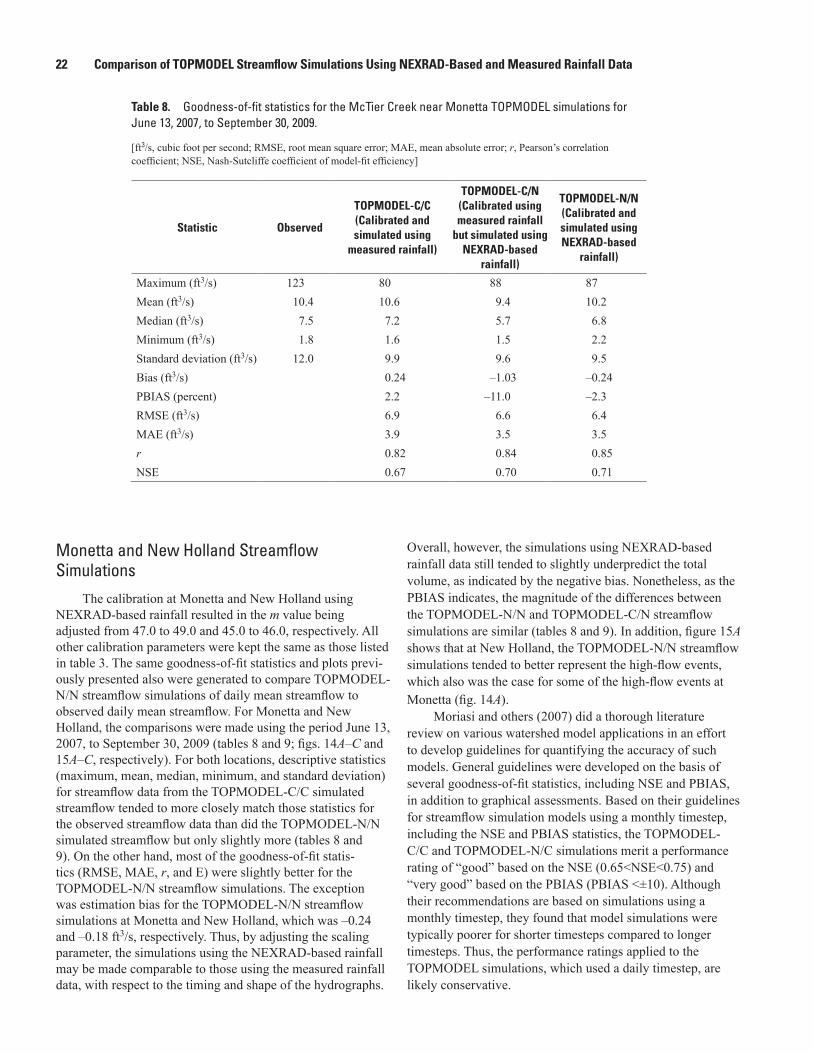
22 Comparison of TOPMODEL Streamflow Simulations Using NEXRAD-Based and Measured Rainfall Data
Monetta and New Holland Streamflow Simulations
The calibration at Monetta and New Holland using NEXRAD-based rainfall resulted in the m value being adjusted from 47.0 to 49.0 and 45.0 to 46.0, respectively. All other calibration parameters were kept the same as those listed in table 3. The same goodness-of-fit statistics and plots previ-ously presented also were generated to compare TOPMODEL-N/N streamflow simulations of daily mean streamflow to observed daily mean streamflow. For Monetta and New Holland, the comparisons were made using the period June 13, 2007, to September 30, 2009 (tables 8 and 9; figs. 14A–C and 15A–C, respectively). For both locations, descriptive statistics (maximum, mean, median, minimum, and standard deviation) for streamflow data from the TOPMODEL-C/C simulated streamflow tended to more closely match those statistics for the observed streamflow data than did the TOPMODEL-N/N simulated streamflow but only slightly more (tables 8 and 9). On the other hand, most of the goodness-of-fit statis-tics (RMSE, MAE, r, and E) were slightly better for the TOPMODEL-N/N streamflow simulations. The exception was estimation bias for the TOPMODEL-N/N streamflow simulations at Monetta and New Holland, which was –0.24 and –0.18 ft3/s, respectively. Thus, by adjusting the scaling parameter, the simulations using the NEXRAD-based rainfall may be made comparable to those using the measured rainfall data, with respect to the timing and shape of the hydrographs.
Overall, however, the simulations using NEXRAD-based rainfall data still tended to slightly underpredict the total volume, as indicated by the negative bias. Nonetheless, as the PBIAS indicates, the magnitude of the differences between the TOPMODEL-N/N and TOPMODEL-C/N streamflow simulations are similar (tables 8 and 9). In addition, figure 15A shows that at New Holland, the TOPMODEL-N/N streamflow simulations tended to better represent the high-flow events, which also was the case for some of the high-flow events at Monetta (fig. 14A).
Moriasi and others (2007) did a thorough literature review on various watershed model applications in an effort to develop guidelines for quantifying the accuracy of such models. General guidelines were developed on the basis of several goodness-of-fit statistics, including NSE and PBIAS, in addition to graphical assessments. Based on their guidelines for streamflow simulation models using a monthly timestep, including the NSE and PBIAS statistics, the TOPMODEL-C/C and TOPMODEL-N/C simulations merit a performance rating of “good” based on the NSE (0.65<NSE<0.75) and “very good” based on the PBIAS (PBIAS <±10). Although their recommendations are based on simulations using a monthly timestep, they found that model simulations were typically poorer for shorter timesteps compared to longer timesteps. Thus, the performance ratings applied to the TOPMODEL simulations, which used a daily timestep, are likely conservative.
Table 8. Goodness-of-fit statistics for the McTier Creek near Monetta TOPMODEL simulations for June 13, 2007, to September 30, 2009.
[ft3/s, cubic foot per second; RMSE, root mean square error; MAE, mean absolute error; r, Pearson’s correlation coefficient; NSE, Nash-Sutcliffe coefficient of model-fit efficiency]
Statistic Observed
TOPMODEL-C/C (Calibrated and simulated using
measured rainfall)
TOPMODEL-C/N (Calibrated using measured rainfall
but simulated using NEXRAD-based
rainfall)
TOPMODEL-N/N (Calibrated and simulated using NEXRAD-based
rainfall)
Maximum (ft3/s) 123 80 88 87Mean (ft3/s) 10.4 10.6 9.4 10.2Median (ft3/s) 7.5 7.2 5.7 6.8Minimum (ft3/s) 1.8 1.6 1.5 2.2Standard deviation (ft3/s) 12.0 9.9 9.6 9.5Bias (ft3/s) 0.24 –1.03 –0.24PBIAS (percent) 2.2 –11.0 –2.3RMSE (ft3/s) 6.9 6.6 6.4MAE (ft3/s) 3.9 3.5 3.5r 0.82 0.84 0.85NSE 0.67 0.70 0.71

TOPMODEL Streamflow Simulations 23
Streamflow Simulations in McTier Creek Subwatersheds
One of the benefits of a watershed model such as TOPMODEL is the ability to simulate streamflow for subwatersheds using the model parameters from a calibrated watershed model. If the subwatershed basin characteristics are similar to those of the calibrated watershed, it is reason-able to assume the parameters from the calibrated watershed will provide acceptable streamflow simulations at ungaged locations. In Feaster and others (2010), the McTier Creek watershed was subdivided into 12 subwatersheds, and stream-flow was simulated for each subwatershed for the period June 13, 2007, to September 30, 2009, using the calibrated TOPMODEL parameters from Monetta and New Holland as well as soil and watershed characteristics from the subwa-tersheds (fig. 5). As a result, the subwatershed models repre-sented separate, individual applications of TOPMODEL. For those simulations, the same measured rainfall data were used for all subwatersheds as were used for the Monetta and New Holland watersheds.
The individual subwatersheds were not gaged, and therefore, no continuous streamflow record was available to compare with the simulated streamflow. Nonetheless, a comparison of the simulated streamflow for each subwa-tershed from the TOPMODEL-C/C and TOPMODEL-N/N models was made to assess the similarity in the simulated hydrographs. As in Feaster and others (2010), streamflow
simulations for subwatersheds also were summed and compared with streamflow simulations for the Monetta and New Holland watersheds to assess overall reasonableness of subwatershed streamflow simulations.
TOPMODEL-C/C and TOPMODEL-N/N streamflow simulations were generated for subwatersheds MA01 to MA12. The streamflow simulations from subwatersheds MA01 to MA06 were summed and compared to the TOPMODEL streamflow simulation at the Monetta gage. The streamflow simulations for subwatersheds MA01 to MA12 were summed and compared to the TOPMODEL simu-lation at the New Holland gage. For the TOPMODEL-C/C streamflow simulations, the total volume of the streamflow simulated for the subwatersheds was about 1 and 3 percent greater than the total volume of the simulations at Monetta and New Holland (figs. 16A and B), respectively. For the TOPMODEL-N/N streamflow simulations, the total stream-flow volume for the subwatersheds was about 1 and 6 percent greater than the total streamflow volume of the TOPMODEL simulations at Monetta and New Holland (figs. 17A and B), respectively.
Plots showing TOPMODEL-C/C and TOPMODEL-N/N streamflow simulations for each subwatershed were generated for the period June 13, 2007, to September 30, 2009 (fig. 18). The plots indicate that the hydrograph shapes tend to be similar with varying deviations in magnitude for particular events. The percent difference for the total streamflow volume for the period simulated at each subwatershed was computed (table 10).
Table 9. Goodness-of-fit statistics for the McTier Creek near New Holland TOPMODEL simulations for June 13, 2007, to September 30, 2009.
[ft3/s, cubic foot per second; RMSE, root mean square error; MAE, mean absolute error; r, Pearson’s correlation coefficient; NSE, Nash-Sutcliffe coefficient of model-fit efficiency]
Statistic Observed
TOPMODEL-C/C (Calibrated and simulated using
measured rainfall)
TOPMODEL-C/N (Calibrated using measured rainfall
but simulated using NEXRAD-based
rainfall)
TOPMODEL-N/N (Calibrated and simulated using NEXRAD-based
rainfall)
Maximum (ft3/s) 163 159 179 177Mean (ft3/s) 21.8 21.5 20.5 21.2Median (ft3/s) 17.0 14.6 12.9 13.8Minimum (ft3/s) 2.6 4.1 3.6 4.7Standard deviation (ft3/s) 19.9 18.8 20.1 19.7Bias (ft3/s) 0.07 –0.94 –0.18
PBIAS (percent) 0.31 –4.6 –0.87
RMSE (ft3/s) 11.1 11.2 10.9
MAE (ft3/s) 6.8 6.9 6.6
r 0.82 0.84 0.85
NSE 0.67 0.67 0.68

24 Comparison of TOPMODEL Streamflow Simulations Using NEXRAD-Based and Measured Rainfall Data
Figure 14. TOPMODEL-C/C and TOPMODEL-N/N streamflow simulations in relation to A, daily mean flows, B, flow-duration curves, and C, single-mass curves at McTier Creek near Monetta (station 02172300) for June 13, 2007, to September 30, 2009. NWS COOP is National Weather Service Cooperative meteorological station.
Figure 15. TOPMODEL-C/C and TOPMODEL-N/N streamflow simulations in relation to observed streamflow for A, daily mean flows, B, flow-duration curves, and C, single-mass curves at McTier Creek near New Holland (station 02172305) for June 13, 2007, to September 30, 2009. NWS COOP is National Weather Service Cooperative meteorological station.
Cum
ulat
ive
daily
mea
n flo
w, i
n cu
bic
feet
per
sec
ond
Daily
mea
n flo
w, i
n cu
bic
feet
per
sec
ond
140130120110100
908070605040302010
0
A. Daily mean flows
1,000
100
10
1
B. Flow-duration curves
10,000
9,000
8,000
7,000
6,000
5,000
4,000
3,000
2,000
1,000
0
C. Single-mass curves
0 10 20 30 40 50Percent of time indicated flow was equaled or exceeded
60 70 80 90 100
2007 2008 2009J J A F M A MS O N D J J J A F M AS O M J J A S ON D J
2007 2008 2009J J A F M A MS O N D J J J A F M AS O M J J A S ON D J
ObservedTOPMODEL (NWS COOP)TOPMODEL (NEXRAD)
EXPLANATION
ObservedTOPMODEL (NWS COOP)TOPMODEL (NEXRAD)
EXPLANATION
ObservedTOPMODEL (NWS COOP)TOPMODEL (NEXRAD)
EXPLANATION
Daily
mea
n flo
w, i
n cu
bic
feet
per
sec
ond
A. Daily mean flows
B. Flow-duration curves
C. Single-mass curves
ObservedTOPMODEL (NWS COOP)TOPMODEL (NEXRAD)
EXPLANATION
ObservedTOPMODEL (NWS COOP)TOPMODEL (NEXRAD)
EXPLANATION
ObservedTOPMODEL (NWS COOP)TOPMODEL (NEXRAD)
Cum
ulat
ive
daily
mea
n flo
w, i
n cu
bic
feet
per
sec
ond
240
220
200
180
160
140
120
100
80
60
40
20
0
1,000
100
10
1
20,000
18,000
16,000
14,000
12,000
10,000
8,000
6,000
4,000
2,000
0
0 10 20 30 40 50Percent of time indicated flow was equaled or exceeded
60 70 80 90 100
2007 2008 2009J J A F M A MS O N D J J J A F M AS O M J J A S ON D J
2007 2008 2009J J A F M A MS O N D J J J A F M AS O M J J A S ON D J

TOPMODEL Streamflow Simulations 25
Figure 16. TOPMODEL-C/C streamflow simulations of daily mean streamflow for June 13, 2007, to September 30, 2009, at A, McTier Creek near Monetta (station 02172300) and the sum of the simu-lated daily mean streamflow for subwatersheds MA01 to MA06, and B, McTier Creek near New Holland (station 02172305) and the sum of the simulated daily mean streamflow for subwatersheds MA01 to MA12.
Figure 17. TOPMODEL-N/N streamflow simulations for June 13, 2007, to September 30, 2009, at A, McTier Creek near Monetta (station 02172300) and the sum of simulated daily mean streamflow for subwatersheds MA01 to MA06, and B, McTier Creek near New Holland (station 02172305) and the sum of simulated daily mean streamflow for subwatersheds MA01 to MA12. NWS COOP is National Weather Service Cooperative meteorological station.
Daily
mea
n flo
w, i
n cu
bic
feet
per
sec
ond
New HollandSum of subwatersheds MA01–MA12
EXPLANATION
MonettaSum of subwatersheds MA01–MA06
EXPLANATION
A. McTier Creek near Monetta
200
180
160
140
120
100
80
60
40
20
0
200
180
160
140
120
100
80
60
40
20
0B. McTier Creek near New Holland
2007
May Aug. Nov. May Aug. Nov.Feb. May Aug. Nov.Feb.
2008 2009

26 Comparison of TOPMODEL Streamflow Simulations Using NEXRAD-Based and Measured Rainfall Data
Figure 18. TOPMODEL-C/C and TOPMODEL-N/N simulated daily mean streamflow at McTier Creek subwatersheds MA01 to MA12 for June 13, 2007, to September 30, 2009.
2007June Aug. Oct. June Aug. Oct.Dec. Feb. Apr. June Aug. Oct. Dec. Feb. Apr.
2008 2009 2007June Aug. Oct. June Aug. Oct.Dec. Feb. Apr. June Aug. Oct. Dec. Feb. Apr.
2008 2009
MA0140
35
30
25
20
15
10
5
0
40
35
30
25
20
15
10
5
0
40
35
30
25
20
15
10
5
0
MA02
MA03 MA04
MA05 MA06
Daily
mea
n flo
w, i
n cu
bic
feet
per
sec
ond
Figure 18.
TOPMODEL (NWS COOP)TOPMODEL (NEXRAD)
EXPLANATION

TOPMODEL Streamflow Simulations 27
Figure 18. Graphs showing TOPMODEL-C/C and TOPMODEL-N/N simulated daily mean streamflow at McTier Creek subwatersheds MA01 to MA12 for June 13, 2007, to September 30, 2009.—Continued
2007June Aug. Oct. June Aug. Oct.Dec. Feb. Apr. June Aug. Oct. Dec. Feb. Apr.
2008 2009 2007June Aug. Oct. June Aug. Oct.Dec. Feb. Apr. June Aug. Oct. Dec. Feb. Apr.
2008 2009
MA07
40
35
30
25
20
15
10
5
0
40
35
30
25
20
15
10
5
0
40
35
30
25
20
15
10
5
0
MA08
MA09 MA10
MA11 MA12
Daily
mea
n flo
w, i
n cu
bic
feet
per
sec
ond
Figure 18. cont.
TOPMODEL (NWS COOP)TOPMODEL (NEXRAD)
EXPLANATION

28 Comparison of TOPMODEL Streamflow Simulations Using NEXRAD-Based and Measured Rainfall Data
Table 10. McTier Creek subwatershed area and percent difference between TOPMODEL-C/C and TOPMODEL-N/N simulated total volume of daily mean streamflow.
[mi2, square mile; C/C, TOPMODEL calibration and simulations done using measured rainfall; N/N, TOPMODEL calibration and simulations done using NEXRAD-based rainfall]
McTier Creek Subwatersheds
MA01 MA02 MA03 MA04 MA05 MA06 MA07 MA08 MA09 MA10 MA11 MA12
Area (mi2) 2.66 6.75 1.46 1.63 0.81 2.31 4.88 2.58 2.40 1.67 0.91 2.59Percent difference
21.8 6.9 0.4 7.1 4.3 0.5 –6.4 –7.9 –10.0 –6.1 –19.3 –12.7
Table 11. Total NEXRAD-based rainfall by subwatershed and differences from total NEXRAD-based rainfall and total NWS COOP rainfall for McTier Creek near New Holland.
[in., inch]
McTier Creek Subwatersheds
MA01 MA02 MA03 MA04 MA05 MA06 MA07 MA08 MA09 MA10 MA11 MA12
Total NEXRAD-based daily rainfall (in.)
82.2 83.8 86.2 85.0 87.5 86.5 93.2 93.7 93.3 90.9 88.6 94.6
Difference from total NEXRAD-based rainfall at New Holland (in.)
–6.4 –4.8 –2.4 –3.6 –1.1 –2.1 4.6 5.1 4.7 2.3 0.0 6.0
Difference from total NWS COOP rainfall at New Holland (in.)
–12.5 –10.9 –8.6 –9.8 –7.2 –8.3 –1.5 –1.0 –1.4 –3.9 –6.1 –0.2
the case for measured data. The data in table 10, however, are presented without taking the absolute value in order to illustrate the direction and magnitude of differences between TOPMODEL-C/C and TOPMODEL-N/N streamflow simula-tions. The percentage differences for subwatersheds MA01 to MA06 are all positive, indicating the total TOPMODEL-C/C simulated streamflow is larger than the total TOPMODEL-N/N simulated streamflow. For subwatersheds MA07 to MA12, the opposite is true with the total volume from the TOPMODEL-N/N streamflow simulations being greater than the TOPMODEL-C/C streamflow simulations. Weighting the percentage differences by area and then summing the values results in an average percentage difference of –0.5 percent.
The differences in the total NEXRAD-based rainfall for the McTier Creek watershed at New Holland (88.6 inches) for the period June 13, 2007, to September 30, 2009, and the total NEXRAD-based rainfall for each subwatershed for the same period are given in table 11. Also listed are the differences in the total NWS COOP rainfall at New Holland (94.7 inches) and the total NEXRAD-based rainfall for each subwatershed.
The percent difference is computed as the absolute value of the difference in the total streamflow volume from the TOPMODEL-C/C streamflow simulations and TOPMODEL-N/N streamflow simulations divided by the average of the two total streamflow volumes and that quantity is multiplied by 100:
PercentDifferencex xx x
=−+
×| |1 2
1 2
2
100 ,
(11)
where x1 is the total simulated flow using measured
rainfall data, and x2 is the total simulated flow using NEXRAD-
based rainfall data.The absolute value of the difference is taken here because the values being compared are both model estimates and, therefore, neither is considered to be more “correct,” as is
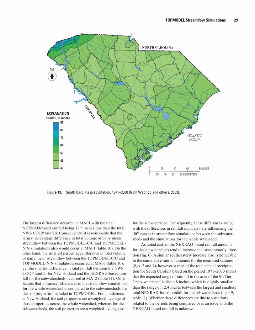
TOPMODEL Streamflow Simulations 29
The largest difference occurred at MA01 with the total NEXRAD-based rainfall being 12.5 inches less than the total NWS COOP rainfall. Consequently, it is reasonable that the largest percentage difference in total volume of daily mean streamflow between the TOPMODEL-C/C and TOPMODEL-N/N simulations also would occur at MA01 (table 10). On the other hand, the smallest percentage difference in total volume of daily mean streamflow between the TOPMODEL-C/C and TOPMODEL-N/N simulations occurred at MA03 (table 10), yet the smallest difference in total rainfall between the NWS COOP rainfall for New Holland and the NEXRAD-based rain-fall for the subwatersheds occurred at MA12 (table 11). Other factors that influence differences in the streamflow simulations for the whole watershed as compared to the subwatersheds are the soil properties included in TOPMODEL. For simulations at New Holland, the soil properties are a weighted-average of those properties across the whole watershed, whereas for the subwatersheds, the soil properties are a weighted-average just
for the subwatershed. Consequently, these differences along with the differences in rainfall input also are influencing the differences in streamflow simulations between the subwater-sheds and the simulations for the whole watershed.
As noted earlier, the NEXRAD-based rainfall amounts for the subwatersheds tend to increase in a southeasterly direc-tion (fig. 6). A similar southeasterly increase also is noticeable in the cumulative rainfall amounts for the measured stations (figs. 2 and 7); however, a map of the total annual precipita-tion for South Carolina based on the period 1971–2000 shows that the expected range of rainfall in the area of the McTier Creek watershed is about 8 inches, which is slightly smaller than the range of 12.4 inches between the largest and smallest total NEXRAD-based rainfall for the subwatersheds (fig. 19; table 11). Whether these differences are due to variations related to the periods being compared or is an issue with the NEXRAD-based rainfall is unknown.
0 20 40 60 80 MILES
0 20 40 60 80 KILOMETERS
88
80
72
64
56
48
40
Rainfall, in inchesEXPLANATION
Figure 19.
ATLANTICOCEAN
NORTH CAROLINA
GEORGIA
N
Figure 19. South Carolina precipitation, 1971–2000 (from Wachob and others, 2009).

30 Comparison of TOPMODEL Streamflow Simulations Using NEXRAD-Based and Measured Rainfall Data
Summary and ConclusionsThe decision to use NEXRAD-based rainfall data or
measured rainfall data in watershed model simulations may be influenced by several factors, such as the number of measured rainfall stations in or around the study watershed, the available rainfall data for the period of interest, the confidence in the accuracy of both the NEXRAD-based and measured data, and geographical considerations. The simple fact that NEXRAD-based data can be generated for a watershed at a finer spatial resolution than the measured data does not necessarily guarantee better results with respect to simulating streamflow. The comparisons in this report also show that although differ-ences in the NEXRAD-based and measured rainfall data exist, calibrating a hydrologic model with the rainfall data that will be used in streamflow simulations generated with that model is important and may result in simulations that are overall similar with respect to magnitude of the goodness-of-fit statistics used to assess those simulations.
Measured rainfall data were compared with NEXRAD-based rainfall data at six NWS COOP stations that surround the McTier Creek watershed. The comparison, using rainfall data for non-zero days at the NWS COOP station locations, indicated that the NEXRAD-based data were lower at all six locations with the total difference in rainfall ranging from –1.3 inches at the Batesburg COOP station to –21.6 inches at the Pelion COOP station. The estimation bias, which is a comparison of the total volume of rainfall for the comparison period, ranged from –1.6 percent at the Batesburg COOP station to –24.1 percent at the Edgefield 3 NNE COOP station. These findings are comparable with results reported for larger watersheds or coverage areas.
A comparison of the number of days with zero and non-zero rainfall for the NWS COOP and NEXRAD-based rainfall for the Monetta and New Holland watersheds indicated that the NEXRAD-based data had fewer days of non-zero rainfall. For the period June 13, 2007, to September 30, 2009 (841 days), the number of non-zero days in the NEXRAD-based data at Monetta and New Holland was 263 and 268, respectively. For the same period, the NWS COOP measured data had 344 days of non-zero rainfall. Thus, at Monetta, there were 31 percent more days for which rainfall was recorded than was indicated in the NEXRAD-based estimates and for New Holland, there were 28 percent more days for which rainfall was recorded than was indicated in the NEXRAD-based estimates. In terms of total rainfall, for the days for which no rainfall was noted in the NEXRAD-based estimates, there was an additional 4.23 and 4.08 inches of recorded rainfall at the NWS COOP stations for Monetta and New Holland, respectively.
Using the calibrated watershed model (TOPMODEL) for McTier Creek, streamflow simulations were made using NEXRAD-based rainfall data and then compared with simula-tions using measured rainfall data at USGS stations 02172300, McTier Creek near Monetta, SC, and 02172305, McTier
Creek near New Holland, SC. Several of the goodness-of-fit statistics that provide numerical comparisons of the timing and shape of simulated and observed streamflow hydrographs indicated similar results from the streamflow simulations using measured and NEXRAD-based rainfall data. However, bias, which is the average of the residuals between the simulated and observed streamflow data, showed that streamflow simulations using the NEXRAD-based rainfall had a nega-tive bias of –1.03 and –0.94 ft3/s, respectively, compared to a bias of 0.07 and 0.24 ft3/s, respectively, using the measured rainfall data. The equivalent percentage biases (PBIAS) were –11.0 and –4.6 percent, respectively, and 0.31 and 2.2 percent, respectively. Given that the comparisons of the measured and NEXRAD-based rainfall at the NWS COOP stations had previously showed a negative bias in the NEXRAD-based data, these result were expected.
As an additional comparison of TOPMODEL simula-tions using the measured and NEXRAD-based rainfall, TOPMODEL was recalibrated using NEXRAD-based rainfall (TOPMODEL-N/N). Although still negative, the recalibra-tion reduced the bias at Monetta and New Holland to –0.24 and –0.18 ft3/s, respectively. Other goodness-of-fit statistics showed similar results as those from the TOPMODEL simulations using measured rainfall data. The comparisons of TOPMODEL simulations using measured and NEXRAD-based rainfall for the McTier Creek watershed indicate that both rainfall datasets provide reasonable results with respect to matching the measured streamflow.
One of the perceived benefits of NEXRAD-based rainfall is the ability to generate a finer-resolution set of input rainfall data for subwatersheds in the simulated watershed. In order to evaluate this benefit, McTier Creek was divided into 12 subwatersheds, and streamflow simulations were generated for each subwatershed using both measured rainfall data and NEXRAD-based rainfall. The streamflow simulations from the subwatersheds upstream from the Monetta gage were summed and compared to the TOPMODEL streamflow simulation at the Monetta gage. The same was done for the subwatersheds upstream from the New Holland gage. For the TOPMODEL simulations using measured rainfall, the total streamflow volume for the subwatersheds was about 1 and 3 percent greater than the total simulated streamflow volumes at the Monetta and New Holland gages, respectively. Using the NEXRAD-based rainfall, the total volumes were about 1 and 6 percent greater, respectively.
A comparison of the variability in the NEXRAD-based rainfall data for the 12 subwatersheds also was made using single-mass curves. The results showed that the total volume of rainfall increased by about 15 percent from subwatershed MA01 to subwatershed MA12. A similar comparison was made of the variability of the total rainfall volume at the six NWS COOP stations. The Pelion station had the largest volume and the Batesburg station had the smallest with about a 25 percent difference between the two. The difference in the total measured rainfall between the Johnston 4SW station and the Batesburg station was about 10 percent. As was true

References Cited 31
with the NEXRAD-based rainfall data, the total volume of the measured rainfall data for the comparison period appeared to increase from north to south although the magnitude of the NEXRAD-based difference (15 percent) occurred over a much smaller distance than the NWS COOP stations. The distance between the most northern and most southern located NWS COOP stations is about 35 miles, whereas the distance from the northern part of the McTier Creek watershed to the southern part is about 9 miles.
Regarding subwatershed simulations, NEXRAD-based estimates provide the opportunity for finer spatial resolution input rainfall data over an area were the rainfall data are known to vary. In smaller watersheds, this variability is likely to be within the uncertainty of the watershed model simula-tions. Nonetheless, where measured rainfall data are limited, NEXRAD-based multisensory precipitation data may provide an effective alternative.
References Cited
Bedient, P.B., Huber, W.C., and Vieux, B.E., 2008, Hydrology and floodplain analysis (4th ed.): Upper Saddle River, N.J., Prentice-Hall, Inc., 816 p.
Beven, K.J., 1997, Distributed hydrological modelling—Applications of the TOPMODEL concept: Chichester, England, John Wiley & Sons Ltd., 356 p.
Beven, K.J., 2001, Rainfall-runoff modelling—The primer: Chichester, England, John Wiley & Sons Ltd., 360 p.
Beven, K.J., and Kirkby, M.J., 1979, A physically based, variable contributing area model of basin hydrology: Hydrological Sciences Bulletin, v. 24, p. 43–69.
Bloxham, W.M., 1976, Low-flow characteristics of streams in the Inner Coastal Plain of South Carolina: South Carolina Water Resources Commission Report No. 5, 28 p.
Bradley, P.M., Burns, D.A., Riva-Murray, Karen, Brigham, M.E., Button, D.T., Chasar, L.C., Marvin-DiPasquale, Mark, Lowery, M.A., and Journey, C.A., 2011, Spatial and seasonal variability of dissolved methylmercury in two stream basins in the eastern United States: Environmental Science & Technology, v. 45, p. 2048–2055, accessed May 25, 2012, at http://pubs.acs.org/doi/pdf/10.1021/es103923j.
Cooke, C.W., 1936, Geology of the Coastal Plain of South Carolina: U.S. Geological Survey Bulletin 867, 196 p.
Crum, T.D., and Alberty, R.L., 1993, The WSR–88D and the WSR–88D Operation Support Facility: Bulletin of the American Meteorological Society, v. 74, no. 9, p. 1669–1687.
Dai, T., Ambrose, R.B., Jr., Alvi, K., Wool, T.A., Manguerra, H., Chokshi, M., Yang, H., and Kraemer, S.R., 2005, Characterizing spatial and temporal dynamics—Develop-ment of a grid-based watershed mercury loading model, in Moglen, G.E., ed., Managing watersheds for human and natural impacts—Engineering, ecological, and economic challenges: Williamsburg, Va., American Society of Civil Engineers, July 19–22, 2005, p. 56.
Doherty, John, 2005, PEST—Model-independent parameter estimation user manual (5th ed.): Watermark Numerical Computing, 336 p.
Dunne, Thomas, and Black, R.D., 1970, Partial area contribu-tions to storm runoff in a small New England watershed: Water Resources Research, v. 6, no. 5, p. 1296–1311.
Eidson, J.P., Lacy, C.M., Nance, Luke, Hansen, W.F., Lowery, M.A., and Hurley, N.M., Jr., 2005, Development of a 10- and 12-digit hydrologic unit code numbering system for South Carolina, 2005: U.S. Department of Agriculture, Natural Resources Conservation Service, 38 p., 1 pl.
Feaster, T.D., Golden, H.E., Odom, K.R., Lowery, M.A., Conrads, P.A., and Bradley, P.M., 2010, Simulation of streamflow in the McTier Creek watershed, South Carolina: U.S. Geological Survey Scientific Investigation Report 2010–5202, 61 p.
Fulton, R.A., Breidenbach, J.P., Seo, D.J., Miller, D.A., and O’Bannon, Timothy, 1998, The WSR–88D rainfall algo-rithm: Weather and Forecasting, v. 13, no. 2, p. 377–395.
Fulton, R.A., Ding, Feng, and Miller, D.A., 2003, Trunca-tion errors in historical WSR–88D rainfall products: 31st American Meteorological Society Conference on Radar Meteorology, Seattle, Wash., Aug. 2003, 4 p.
Griffith, G.E., Omernik, J.M., Comstock, J.A., Schafale, M.P., McNab, W.H., Lenat, D.R., MacPherson, T.F., Glover, J.B., and Shelburne, V.B., 2002, Ecoregions of North Carolina and South Carolina: U.S. Geological Survey color poster with map, scale 1:1,500,000.
Habib, E., Larson, B.F., and Graschel, J., 2009, Validation of NEXRAD multisensory precipitation estimates using an experimental dense rain gauge network in south Louisiana: Journal of Hydrology, v. 373, p. 463–478.
Hardegree, S.P., Van Vactor, S.S., Levison, D.H., and Winstral, A.H., 2008, Evaluation of NEXRAD radar precipitation products for natural resource applications: Rangeland Ecology & Management, v. 61, no. 3, p. 346–353.
Helsel, D.R., and Hirsch, R.M., 1995, Studies in environ-mental science, in Statistical methods in water resources: Amsterdam, Elsevier Science, v. 49, 529 p.

32 Comparison of TOPMODEL Streamflow Simulations Using NEXRAD-Based and Measured Rainfall Data
Hornberger, G.M., Raffensperger, J.P., Wiberg, P.L., and Eshleman, K.N., 1998, Elements of physical hydrology: Baltimore, Md., The John Hopkins University Press, 312 p.
Janssen, P.H.M., and Heuberger, P.S.C., 1993, Calibration of process-oriented models: Ecological Modelling, v. 83, p. 55–66.
Jayakrishnan, R., Srinivasan, R., and Arnold, J.G., 2004, Comparison of raingage and WSR–88D Stage III precipita-tion data over the Texas-Gulf Basin: Journal of Hydrology, v. 292, p. 135–152.
Kennen, J.G., Kauffman, L.J., Ayers, M.A., Wolock, D.M., and Colarullo, S.J., 2008, Use of an integrated flow model to estimate ecologically relevant hydrologic characteristics at stream biomonitoring sites: Ecological Modelling, v. 211, p. 57–76.
Krause, P., Boyle, D.P., and Bäse, F., 2005, Comparison of different efficiency criteria for hydrological model assess-ment: Advances in Geosciences, v. 5, p. 89–97.
Legates, D.R., and McCabe, G.J., Jr., 1999, Evaluating the use of “goodness-of-fit” measures in hydrologic and hydrocli-matic model validation: Water Resources Research, v. 35, no. 1, p. 233–241.
Maidment, D.R., 1993, Handbook of hydrology: New York, McGraw-Hill, Inc., 1,424 p.
Mizzell, H.P., 1999, Comparison of WSR–88D derived rainfall estimates with gauge data in Lexington County, South Carolina: University of South Carolina, Department of Geography, Master’s thesis, accessed November 14, 2011, at http://www.dnr.sc.gov/climate/sco/Publications/thesis/thesis.html.
Moon, J., Srinivasan, R., and Jacobs, J.H., 2004, Stream flow estimation using spatially distributed rainfall in the Trinity River Basin, Texas: Transactions of the American Society of Agricultural Engineers, v. 47, no. 5, p. 1445–1451.
Moriasi, D.N., Arnold, J.G., Van Liew, M.W., Bingner, R.L., Harmel, R.D., and Veith, T.L., 2007, Model evaluation guidelines for systematic quantification of accuracy in watershed simulations: Transactions of the American Society of Agricultural and Biological Engineers, v. 50, no. 3, p. 885–900.
Nash, J.E., and Sutcliffe, J.V., 1970, River flow forecasting through conceptual models—Part I. A discussion of prin-ciples: Journal of Hydrology, v. 10, p. 282–290.
National Climatic Data Center, 1996, A comparison of NEXRAD rainfall estimates with recorded amounts: U.S. Department of Commerce, National Climatic Data Center Technical Report 96–03, 28 p.
National Climatic Data Center, 2006, Data documentation for data set 3200 (DSI–3200), surface land daily cooperative summary of the day: Asheville, N.C., National Climatic Data Center, 19 p., accessed May 25, 2012, at http://rda.ucar.edu/datasets/ds510.0/docs/2006jun.td3200.html.
Nelson, B.R., Seo, D.-J., and Kim, Dongsoo, 2010, Multi-sensor precipitation reanalysis: Journal of Hydrometeo-rology, v. 11, no. 3, p. 666–682.
Norman, G.R., and Streiner, D.L., 1997, PDQ statistics: St. Louis, Mo., Mosby-Year Book, Inc., 188 p.
Seo, D.J., and Breidenbach, J.P., 2002, Real-time correction of spatially nonuniform bias in radar rainfall data using rain gauge measurements: Journal of Hydrometeorology, v. 3, no. 2, p. 93–111.
Sexton, A.M., Sadeghi, A.M., Zhang, X., Srinivasan, R., and Shirmonhammadi, A., 2010, Using NEXRAD and rain gauge precipitation data for hydrologic calibration of SWAT in a Northeastern watershed: Transactions of the American Society of Agricultural and Biological Engineers, v. 53, no. 5, p. 1501–1510.
Shepard, Donald, 1968, A two-dimensional interpolation function for irregularly-spaced data, Proceedings of the 1968 23rd Association for Computing Machinery (ACM) National Conference: Brandon Systems, Association for Computing Machinery, p. 517–524.
Smith, J.A., Seo, D.J., Baeck, M.L., and Hudlow, M.D., 1996, An intercomparison study of NEXRAD precipita-tion estimates: Water Resources Research, v. 32, no. 7, p. 2035–2045.
Tetra Tech, 2006, Development of second-generation of mercury watershed simulation technology—Grid-Based Mercury Model Version 2.0, User's Manual: Fairfax, Va., Tetra Tech.
U.S. Geological Survey, 2007, Facing tomorrow’s chal-lenges—U.S. Geological Survey science in the decade 2007–2017: U.S. Geological Survey Circular 1309, 70 p.
Wachob, Andrew, Park, A.D., and Newcome, Roy, Jr., eds., 2009, South Carolina state water assessment (2d ed.): Columbia, South Carolina Department of Natural Resources, Land, Water and Conservation Division, 407 p.
Westcott, N.E., 2009, Differences in multi-sensor and rain-gauge precipitation amounts: Proceedings of the Institution of Civil Engineers, Water Management, v. 162, p. 73–81.
Westcott, N.E., Knapp, H.V., and Hilberg, S.D., 2008, Comparison of gage and multisensory precipitation esti-mates over a range of spatial and temporal scales in the Midwestern United States: Journal of Hydrology, v. 351, p. 1–12.
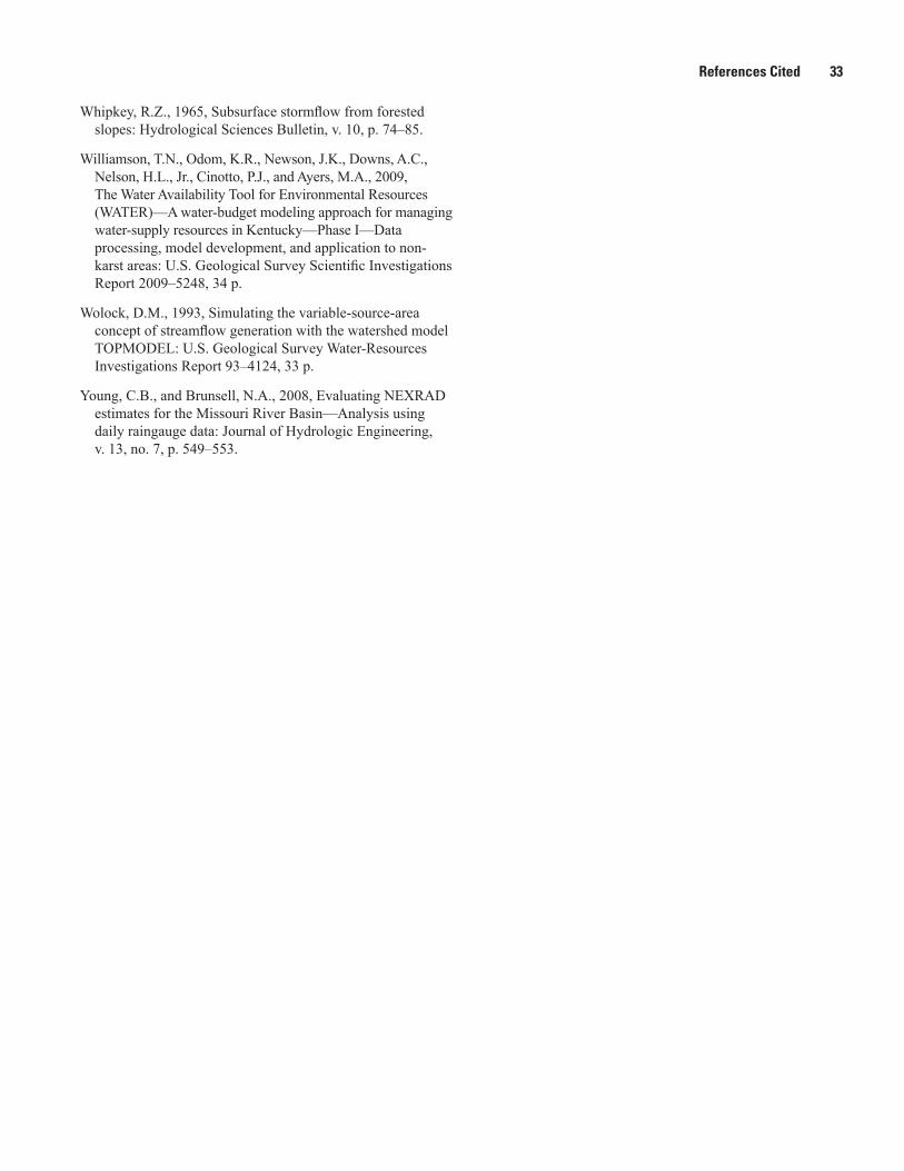
References Cited 33
Whipkey, R.Z., 1965, Subsurface stormflow from forested slopes: Hydrological Sciences Bulletin, v. 10, p. 74–85.
Williamson, T.N., Odom, K.R., Newson, J.K., Downs, A.C., Nelson, H.L., Jr., Cinotto, P.J., and Ayers, M.A., 2009, The Water Availability Tool for Environmental Resources (WATER)—A water-budget modeling approach for managing water-supply resources in Kentucky—Phase I—Data processing, model development, and application to non-karst areas: U.S. Geological Survey Scientific Investigations Report 2009–5248, 34 p.
Wolock, D.M., 1993, Simulating the variable-source-area concept of streamflow generation with the watershed model TOPMODEL: U.S. Geological Survey Water-Resources Investigations Report 93–4124, 33 p.
Young, C.B., and Brunsell, N.A., 2008, Evaluating NEXRAD estimates for the Missouri River Basin—Analysis using daily raingauge data: Journal of Hydrologic Engineering, v. 13, no. 7, p. 549–553.

Manuscript approved June 14, 2012
For more information about this publication, contact:Toby Feaster, HydrologistUSGS South Carolina Water Science CenterClemson Field Office405 College Ave., Suite 200Clemson, SC 29631phone: (864) 656-6747e-mail: [email protected]
Or visit the South Carolina Water Science CenterWeb site at: http://sc.water.usgs.gov
Edited by Kay P. NaugleIllustrations by Jeffrey L. CorbettLayout by Mike G. DeaconCover design concept by James R. Douglas
A PDF version of this publication is available online athttp://pubs.usgs.gov/sir/2011/5180


Feaster and others—Com
parison of TOPMODEL Stream
flow Sim
ulations Using NEXRAD-Based and M
easured Rainfall Data—Scientific Investigations Report 2012–5120


