
Comparative Life Cycle Assessment of hemp and cotton
fibres used in Chinese textile manufacturingVergelijkende Life Cycle Assessment van hennep- en katoenvezels gebruikt in de Chinese
textielindustrie
juni 2015
Promotoren:
Prof. Erik Mathijs
Departement Aard- en Omgevingswetenschappen
Afdeling Bio-Economie
Ir. Wouter Achten
Departement Aard- en Omgevingswetenschappen
Afdeling Bos, Natuur en Landschap
Masterproef voorgedragen
tot het behalen van het diploma van
Master of science in de bio-ingenieurswetenschappen:
landbouwkunde
Hannes Van Eynde

"Dit proefschrift is een examendocument dat na de verdediging niet meer werd gecorrigeerd
voor eventueel vastgestelde fouten. In publicaties mag naar dit proefwerk verwezen worden
mits schriftelijke toelating van de promotor, vermeld op de titelpagina."

I
ACKNOWLEDGEMENTS First and foremost I would like to give my sincere gratitude to professor Erik Mathijs
for accepting my thesis research proposal as promoter and for the support and
guidance in developing the proposal and ultimately this thesis. This master thesis
started out as an idea already in May 2013. I would like to thank professor Wannes
Keulemans, who I contacted back then regarding the subject of hemp textiles, for
supporting me in developing my own research subject and for referring me to Erik.
Special thanks also to professor Wouter Achten, co-promoter, for the valuable input
and support. For all the day-to-day guidance, methodological advice, corrections, etc.
I thank Bernd Annaert, whom I could count on during the past year. Other professors
to thank for their input are prof. Danny Bylemans, prof. Chris Michiels, prof. Eddie
Schrevens, prof. Ilse Smets and prof. Bart van der Bruggen.
As I knew beforehand, finding the right data would be the key issue in developing this
thesis. Therefore special acknowledgements should be given to everyone from Nova-
Institute, and by extension the European Industrial Hemp Association: Michael Carus,
Dominik Vogt and Roland Essel, thank you for giving me the opportunity to network
in the hemp industry at the EIHA conference and for all advice and ideas during my
visits to Nova-Institute. Special thanks go to Martha Barth for our valuable
collaboration the past year. Her personal feedback, data and advice were very
valuable in completing this thesis. For providing me with data and information I also
thank Dr. Stefano Amaducci, Dr. Tyan Changyan, Veronique De Mey, Dr. Bijay
Ghosh, Dr. Hans-Jörg Gusovius, Dr. Fei-Hu Liu, Lawrence Serbin, Dr. Tang
Shouwei, Dr. Natascha Van der Velden and Hayo Van der Werf. Special thanks go to
the people of the Chinese textile mill that put a lot of effort in providing me with the
necessary data. This company prefers to remain anonymous.
A lot of gratitude goes out to Robert Hertel. Without his advice on hemp textiles this
thesis would have been a lot harder. If not impossible.
Finally, I would like to thank everyone who has been part of 5 beautiful years at the
faculty of bioscience engineering. I’ve had the time of my life and that is thanks to
you! This includes my girlfriend, my parents, my family, my housemates and the
entire LBK student association, among many others. Thank you.

II
ABSTRACT This study aims at assessing the environmental impacts of the production of hemp
textiles compared to those of cotton textiles. The idea originated from popular
literature and hemp textile marketing, where the fibre is presented as the miraculously
sustainable alternative to cotton fibre, which is generally considered as a crop with
major environmental impact. Because all hemp textiles are currently produced in
China, the scope of this study is limited to comparing hemp from the Heilongjiang
province to Chinese cotton from the Yellow River Region. The focus of this study is
to uncover the intrinsic differences of hemp and cotton fibres and their processing
technologies and the influence this has on the total environmental impact of textile
manufacturing. Using the life cycle assessment methodology an objective and parallel
comparison is made of both hemp and cotton textiles. The crop cultivation stage is
assessed in detail per kg fibre. Two scenarios per crop are used: one for the common
agricultural practices and one for recommended practices. Additionally, the textile
manufacturing process is assessed up to 1 kg greige fabric, ready for further dyeing
(cradle-to-gate). Here a reference scenario of cotton is constructed with data from
scientific literature and three hemp scenarios are constructed based on data from an
anonymous Chinese textile mill.
The cultivation of hemp has significantly less environmental impact compared to
cotton. Regarding climate change, acidification, eutrophication and several toxicity
categories the impact of hemp is far lower than that of cotton. Hemp also uses only
half of the land. This only applies to fibres used in technical applications like
biocomposites. The hemp textiles used in textiles are further processed, called
degumming. Adding this process to the cultivation scenario makes that degummed
fibre have a higher impact in every relevant impact category except for marine
eutrophication and terrestrial ecotoxicity. Much of the impact is related to the energy
use in the degumming process. This is therefore the absolute environmental hotspot
for hemp fibres. Comparing the fabric scenarios shows that there is no considerable
technical difference when adding hemp to cotton fabrics except for the degumming
process. Again marine eutrophication is the only impact category with a higher impact
for cotton fabrics. This is partly because the contribution of fibre production to the
total impact is fairly limited.

III
NEDERLANDSTALIGE SAMENVATTING Het doel van deze studie is om de milieu impact van henneptextielproductie te
vergelijken met de impact van katoentextiel. Het idee is afgeleid uit de populaire
literatuur en de huidige marketing rond hennep. Hierin wordt hennep omschreven als
hét duurzame alternatief voor katoenvezel. Katoen wordt namelijk algemeen
beschouwd als een gewas met grote gevolgen voor het milieu. Deze studie wordt
beperkt tot een vergelijking van henneptextiel uit de Heilongjiang provincie, China,
met katoen uit de Gele Rivier-vallei omdat alle productie van henneptextiel
momenteel plaatsvindt in China. Het ultieme doel hierbij is om de intrinsieke
verschillen tussen hennep- en katoenvezel en de nodige bewerkingsstappen bloot te
leggen en de gevolgen hiervan aangaande de milieu impact te kwantificeren. Hiervoor
zal de life cycle assessment, of LCA, methodologie gebruikt worden. Het stadium van
de vezelproductie wordt vergeleken op basis van 1 kg vezel. Hiervoor zijn twee
verschillende scenario’s opgesteld per vezel: één voor de huidige landbouwpraktijken
en één voor de aangeraden praktijken. Verder wordt het hele productieproces
vergeleken op basis van 1 kg geweven stof, klaar om te verven. Een referentiescenario
van katoen en drie verschillende hennepproductiescenario’s worden hierbij gebruikt.
Deze laatste zijn gebaseerd op data van een anonieme, Chinese textielproducent.
De productie van hennepvezel heeft een beduidend lagere milieu impact dan die van
katoen en dit zowel voor klimaatsverandering, verzuring, eutrofiëring en
verschillende toxiciteitscategorieën. Ook gebruikt hennepproductie slechts de helft
van het land vergeleken met katoenvezels. Deze vergelijking past echter enkel voor
technische vezelapplicaties zoals bio-composietmaterialen. Hennepvezels in textiel
worden verder verwerkt met een ‘degummingproces’. Wanneer de impact van dit
proces wordt toegevoegd aan het vezelproductiescenario, is de impact van verwerkte
hennepvezels hoger dan die van katoen voor alle impactcategorieën behalve mariene
eutrofiëring en bodemtoxiciteit. Het merendeel van de impact is gerelateerd aan
energieverbruik binnen het degummingproces. Dit is dan ook de absolute hot spot
voor in de milieu impact van hennepvezels. Uit het vergelijken van de stofscenario’s
blijkt dat er geen belangrijke verschillen zijn tussen hennep- en katoentextielproductie
op het degummingproces na. Ook in dit totaal is mariene eutrofiëring de enige
relevante impact categorie waarvoor katoen een hogere impact heeft. Dit is deels het
gevolg van het relatief kleine aandeel van vezelproductie in de totale milieu impact.

IV
GLOSSARY ALO Agricultural land occupation
C2Ga Cradle-to-gate
C2Gr Cradle-to-grave
CC Climate change
CED Cumulative energy demand
COD Chemical oxygen demand
CP Common practices
ET Evapotranspiration
EU Energy use
FD Fossil resource depletion
FE Freshwater eutrophication
FET Freshwater ecotoxicity
Ga2Ga Gate-to-gate
GAP Good agricultural practices
GHG Greenhouse gas
GOT Ginning outturn
GWP Global warming potential
HT Human toxicity
IR Ionizing radiation
ME Marine eutrophication
MET Marine ecotoxicity
MRD Mineral resource depletion
NLT Natural land transformation
Nm Metric count number
OD Ozone depletion
PMF Particulate matter formation
POF Photochemical oxidant formation
TA Terrestrial acidification
TET Terrestrial ecotoxicity
THC Delta-9-tetrahydrocannabidiol
ULO Urban land occupation
USDA United States Department of Agriculture
WD Water depletion
YRR Yellow River Region

V
LIST OF TABLES Table 1: Overview of economically important cotton species. ............................................................... 14 Table 2: Ginning outturn (GOT) from gins in different countries and sources. ..................................... 18 Table 3: Comparison between two cotton CED assessments indicating major differences. .................. 28 Table 4: Summary of the major contributions to CED, GWP, EP and AP in fibre production. ............. 30 Table 5: Cradle-to-gate product LCAs of cotton products. ..................................................................... 34 Table 6: Main emissions and emission factors coming directly from fertilizer use. .............................. 48 Table 7: Comparison of the energy-intensity of the European and Chinese textile industry ................. 50 Table 8: LCI of the fibre preparation and spinning process of scenario R. ............................................ 51 Table 9: LCI of the sizing and weaving process of scenario R. .............................................................. 52 Table 10: LCI of the degumming process in scenario A and B. ............................................................. 53 Table 11: LCI of the carding process in scenario A and B. .................................................................... 54 Table 12: LCI of the cotton carding process in scenario A. .................................................................... 54 Table 13: LCI of the carding process in scenario C. ............................................................................... 54 Table 14: LCI of the bleaching process in scenario C. ........................................................................... 55 Table 15: LCI of the drawing process in scenario A, B and C. .............................................................. 55 Table 16: LCI of the dry ring spinning process in scenario A and B. ..................................................... 56 Table 17: LCI of the wet ring spinning process in scenario C. ............................................................... 56 Table 18: LCI of the sizing process in scenario A, B and C. .................................................................. 56 Table 19: LCI of the weaving process in scenario A, B and C. .............................................................. 57 Table 20: Chinese energy production mix. ............................................................................................. 57 Table 21: Sensitivity analysis of cotton CP scenario. ............................................................................. 73 Table 22: Sensitivity analysis of hemp CP scenario. .............................................................................. 73 Table 23: Sensitivity analysis of scenario R. .......................................................................................... 74 Table 24: Sensitivity analysis of scenario A. .......................................................................................... 74 Table 25: Sustainability assessments of both cotton and hemp per comparable functional units. ....... 103 Table 26: Summary of all impact categories and characterization factors of the ReCiPe method. ...... 105 Table 27: Calculation of the average ginning output. ........................................................................... 106 Table 28: Calculation of seedcotton yield. ............................................................................................ 106 Table 29: Calculation of the economic allocation between cotton fibre and seed. ............................... 106 Table 30: Calculation of the pesticide use in cotton cultivation. .......................................................... 107 Table 31: Calculation of the fertilizer input in cotton cultivation. ........................................................ 107 Table 32: Comparison of the YRR climate with that of southeastern US cotton-growing regions. ..... 108 Table 33: Calculation of the minimum irrigation used in YRR cotton cultivation. .............................. 108 Table 34: Calculation of the average seed use in cotton cultivation. .................................................... 108 Table 35: Calculation of the low-density polyethylene film used in cotton production. ...................... 109 Table 36: Calculation of the total average mechanization in YRR. ...................................................... 109 Table 37: Comparison of a hand tractor with a normal tractor. ............................................................ 109 Table 38: Calculation of on-farm fuel use in cotton cultivation. .......................................................... 110

VI
Table 39: Calculation of the electricity consumption in cotton ginning. .............................................. 110 Table 40: Calculation of the gas consumption in cotton ginning. ......................................................... 111 Table 41: Calculation of the NMVOC emissions from cotton cultivation. .......................................... 111 Table 42: Calculation of the ammonia emissions from cotton cultivation. .......................................... 111 Table 43: Calculation of the nitric oxides emissions from cotton cultivation. ..................................... 112 Table 44: Calculation of the nitrate emissions from cotton cultivation. ............................................... 112 Table 45: Calculation of the nitrous oxide emissions from cotton cultivation. .................................... 113 Table 46: Calculation of the phosphate emissions from cotton cultivation. ......................................... 114 Table 47: Calculation of the carbon dioxide emissions from cotton cultivation. ................................. 114 Table 48: Calculation of the heavy metal emissions from cotton cultivation. ...................................... 115 Table 49: Comparison of assumed environmental fates of pesticides in cotton cultivation. ................ 116 Table 50: Calculation of the pesticide emissions from cotton cultivation. ........................................... 116 Table 51: Calculation of the emissions from fuel use in cotton cultivation. ......................................... 117 Table 52: Comparison of hemp yields with distribution of fibre and shivs. ......................................... 118 Table 53: Calculation of hemp yield in Heilongjiang province. ........................................................... 118 Table 54: Calculation of the economic allocation between hemp fibre and shivs. ............................... 118 Table 55: Calculation of the pesticide use in hemp cultivation. ........................................................... 119 Table 56: Comparison of the fertilizer input in GAP and CP hemp cultivation scenarios. .................. 119 Table 57: Calculation of the seed used in hemp cultivation. ................................................................ 119 Table 58: Calculation of the on-farm fuel use in hemp cultivation. ..................................................... 120 Table 59: Calculation of the electricity consumption of hemp scutching. ............................................ 120 Table 60: Calculation of the NMVOC emissions from hemp cultivation. ........................................... 121 Table 61: Calculation of the ammonia emissions from hemp cultivation. ........................................... 121 Table 62: Calculation of the nitric oxides emissions from hemp cultivation. ...................................... 121 Table 63: Calculation of the nitrous oxide emissions from hemp cultivation. ..................................... 122 Table 64: Calculation of the nitrate emissions from hemp cultivation. ................................................ 123 Table 65: Calculation of the phosphate emissions from hemp cultivation. .......................................... 123 Table 66: Calculation of the carbon dioxide emissions from hemp cultivation. .................................. 124 Table 67: Calculation of the heavy metal emissions from hemp cultivation. ....................................... 125 Table 68: Comparison of assumed environmental fates of pesticides in hemp cultivation. ................. 126 Table 69: Emissions from pesticides in hemp cultivation. ................................................................... 126 Table 70: Calculation of emissions from fuel use in hemp cultivation. ................................................ 126 Table 71: Calculation of the nitrogen emissions from hemp retting. .................................................... 127 Table 72: LCI of two scenarios for one hectare cotton production. ...................................................... 128 Table 73: LCI of two scenarios for one hectare hemp production. ....................................................... 129 Table 74: Calculation of the electricity consumption in cotton yarn spinning. .................................... 130 Table 75: Calculation of the material flows in cotton yarn spinning. ................................................... 131 Table 76: Calculation of the COD removed in treatment and emitted from cotton sizing. .................. 132 Table 77 Calculation of the electricity consumption in cotton fabric weaving. ................................... 132 Table 78: Calculation of the material flows in cotton fabric weaving. ................................................. 133

VII
Table 79: Summary of the uncertainty ranking of the data in the hemp LCI. ...................................... 133 Table 80: Summary of the uncertainty ranking of the data in the cotton LCI. ..................................... 134 Table 81: Calculation of the material flow in the spinning process of scenario A. .............................. 135 Table 82: Calculation of the material efficiency in the hemp carding process in scenario A and B. ... 135 Table 83: Calculation of the material flow in the spinning process of scenario C. .............................. 136 Table 84: Calculation of the material efficiency in the hemp carding process in scenario C. .............. 136 Table 85: Calculation of the heating energy used in hemp degumming and bleaching. ...................... 137 Table 86: Calculation of the material flow in hemp degumming and bleaching. ................................. 137 Table 87: Calculation of the COD removed in treatment and emitted from the degumming. .............. 138 Table 88: Calculation of the economic allocation of the hemp carding process. ................................. 138 Table 89: Calculation of the COD removed in treatment and emitted from sizing wastewater. .......... 139 Table 90: Calculation of the electricity consumption in weaving in scenario A, B and C. .................. 139 Table 91: Characterization output from Simapro of 1 kg scutched hemp fibre in the CP scenario. ..... 140 Table 92: Characterization output from Simapro of 1 kg ginned cotton fibre in the CP scenario. ....... 140 Table 93: Characterization output of 1 kg degummed hemp and ginned cotton fibre. ......................... 142 Table 94: Characterization output of the degumming of hemp fibre per kg output. ............................ 142 Table 95: Characterization output from Simapro of scenario R. .......................................................... 143 Table 96: Characterization output from Simapro of scenario A. .......................................................... 144 Table 97: Characterization output from Simapro of scenario B. .......................................................... 144 Table 98: Characterization output from Simapro of scenario C. .......................................................... 145 Table 99: Back-of-the-envelope calculations of CO2-sequestration in hemp and cotton fibres. ......... 145

VIII
LIST OF FIGURES Figure 1: Cotton production: World and top three countries. ................................................................. 19 Figure 2: Flow chart of hemp and cotton fibre processing into sliver and ultimately yarn. ................... 20 Figure 3: Natural fibre processing qualities and related end-uses. ......................................................... 23 Figure 4: Summary of cumulative energy demand and global warming potential per kg fibre. ............ 27 Figure 5: Summary of eutrophication and acidification potential per kg of hemp and cotton fibre. ...... 29 Figure 6: Cumulative Energy Demand and Global Warming Potential for yarn and fabric. .................. 32 Figure 7: Distribution of CED, GWP and ReCiPe impact in cotton fabric production. ......................... 34 Figure 8: Impact distribution of different cradle-to-grave Life Cycle Assessments of cotton. .............. 35 Figure 9: The four phases in LCA methodology. ................................................................................... 37 Figure 10: Graphic representation of the LCA scope in the textile value chain. .................................... 39 Figure 11: System boundaries of the comparative lifecycle assessment. ............................................... 40 Figure 12: Normalization of 1 kg hemp and cotton fibre produced in China. ........................................ 59 Figure 13: Characterization of the impact categories in hemp and cotton production. .......................... 61 Figure 14: Impact comparison GAP and CP scenarios in hemp and cotton production. ........................ 63 Figure 15: The impact comparison per kg of cotton and degummed hemp fibre. .................................. 65 Figure 16: Normalization of 1 kg fabric production in four scenarios. .................................................. 66 Figure 17: Characterization of fabric scenarios R, A, B and C. .............................................................. 70 Figure 18: The impact comparison per kg of cotton and degummed hemp fibre. .................................. 78 Figure 19: The relative impact difference of substituting scenario R for A. .......................................... 82 Figure 20: Agricultural land occupation of hemp and cotton. .............................................................. 142 Figure 21: Agricultural land occupation of four fabric scenarios. ........................................................ 145

IX
TABLE OF CONTENTS 1 INTRODUCTION ........................................................................................................... 1
1.1 A HISTORY OF HEMP .................................................................................................................. 1
1.2 THE RISE OF COTTON AND MAN-‐MADE FIBRES ...................................................................... 1
1.3 THE QUESTION OF SUSTAINABILITY ........................................................................................ 2
1.4 A NEW DAWN FOR HEMP .......................................................................................................... 2
1.5 HEMP AS A TEXTILE FIBRE ........................................................................................................ 3
1.6 LIFE CYCLE ASSESSMENT .......................................................................................................... 4
1.7 RESEARCH OBJECTIVES AND THESIS OUTLINE ....................................................................... 4
2 STATE OF THE ART .................................................................................................... 7
2.1 HEMP ........................................................................................................................................... 7 2.1.1 Botanical description ........................................................................................................... 7 2.1.2 Cultivation ........................................................................................................................... 9
2.2 COTTON .................................................................................................................................... 13 2.2.1 Botanical description ......................................................................................................... 13 2.2.2 Cultivation ......................................................................................................................... 14
2.3 NATURAL FIBRES .................................................................................................................... 20 2.3.1 Processing of hemp and cotton .......................................................................................... 20 2.3.2 Current use ......................................................................................................................... 23
2.4 SUSTAINABILITY EVALUATION OF HEMP AND COTTON ...................................................... 24 2.4.1 Type of sustainability assessments .................................................................................... 24 2.4.2 Cradle-to-gate: Crop cultivation ........................................................................................ 25 2.4.3 Cradle-to-gate: Yarn and fabric manufacturing ................................................................ 31 2.4.4 Cradle-to-gate and cradle-to-grave: Product LCA ............................................................ 34 2.4.5 State-of-the-art conclusion ................................................................................................ 35
3 MATERIALS AND METHODS .................................................................................. 37
3.1 INTRODUCTION TO THE METHODOLOGICAL ASPECTS OF LCA ......................................... 37 3.1.1 Four phases of LCA ........................................................................................................... 37 3.1.2 Allocation methods ............................................................................................................ 38
3.2 GOAL AND SCOPE .................................................................................................................... 38 3.2.1 Goal and system boundaries .............................................................................................. 38 3.2.2 Functional unit and LCA scenarios ................................................................................... 49 3.2.3 Data collection and quality ................................................................................................ 41 3.2.4 Applied methodology ........................................................................................................ 41
3.3 LIFE CYCLE INVENTORY ......................................................................................................... 42

X
3.3.1 Subsystem 1A and 1B: Cotton and hemp fibre production ............................................... 43 3.3.2 Subsystem 2: Textile mill cotton scenario R ..................................................................... 50 3.3.3 Subsystem 2: Textile mill hemp scenario A, B and C ....................................................... 52 3.3.4 Background system: Input production ............................................................................... 57
4 RESULTS AND DISCUSSION .................................................................................... 59
4.1 LIFE CYCLE IMPACT ANALYSIS ............................................................................................... 59 4.1.1 Hemp and cotton fibre production ..................................................................................... 59 4.1.2 Scenario R, A, B and C ..................................................................................................... 65 4.1.3 Sensitivity analysis ............................................................................................................ 72
4.2 INTERPRETATION ................................................................................................................... 74 4.2.1 Hemp and cotton fibre production ..................................................................................... 74 4.2.2 Scenario R, A, B and C ..................................................................................................... 82 4.2.3 Limitations to the LCA ...................................................................................................... 86
5 CONCLUSION .............................................................................................................. 89
BIBLIOGRAPHY.................................................................................................................91
APPENDIX 1 TEXTILE LIFE CYCLE ASSESSMENTS .......................................... 103
APPENDIX 2 LCIA IMPACT CATEGORIES ........................................................... 105
APPENDIX 3 LCI CALCULATIONS FOR SUBSYSTEM 1A ................................. 106
APPENDIX 4 LCI CALCULATIONS FOR SUBSYSTEM 1B ................................. 118
APPENDIX 5 LCI OF SUBSYSTEM 1A AND 1B .................................................... 128
APPENDIX 6 DATA QUALITY ASSESSMENT ...................................................... 130
APPENDIX 7 LCI CALCULATIONS FOR SUBSYSTEM 2 R ................................ 132
APPENDIX 8 LCI CALCULATIONS FOR SUBSYSTEM 2 A, B AND C .............. 136
APPENDIX 9 OUTPUT RECIPE MODELING FROM SIMAPRO ........................ 140
APPENDIX 10 BIOGENIC CARBON SEQUESTRATION ....................................... 146

1
1 INTRODUCTION
1.1 A history of hemp
Evidence for the use of hemp in paper and ropes dating back to 6000 BC has been
found in China. References on medicinal use, hemp textiles and eating hemp seeds
later on are abundant in Chinese archaeological sites. Over time, the use of the crop
spread from the Far East towards India, the Middle East and arriving in Europe by
2000 BC (Allegret 2013). Ever since, the uses of hemp multiplied to ultimately
become one of the most important resources for paper, textiles, ropes and canvas
throughout the entire European continent. Hemp was of major strategic importance to
the European powers of that time, as it was a key component of sailing ships that
dominated naval exploration from the 15th to the 19th century (the word ‘canvas’ is
derived form the old French ‘chanevaz’ literally ‘made from hemp’). The slow demise
of hemp sets in with the first steam ships in 1830, the rise of wood-based paper in
1850 and ultimately the breakthrough and competition of cotton for textiles
throughout the 1800s, all fuelled by the rise of cheap fossil energy (Allegret 2013). At
beginning of the 20th century, the United States experienced a sudden rise of the drug
marihuana, derived from the same species of plants. This ultimately led to the
Marihuana Tax Act labelling hemp as a narcotic drug in 1937 (Johnson 2013). This
effectively banned hemp cultivation from the United States and destroyed the
domestic hemp industry (Smith-Heisters 2008). After World War II the US imposed
their view on hemp and marihuana in the UN, prohibiting the cultivation and
possession of cannabis (Johnson 2013).
1.2 The rise of cotton and man-made fibres
From the beginning of the 19th century, when the mechanical cotton thresher was
invented, cotton became real competition for hemp fibres (Allegret 2013). Cotton was
naturally softer than the strong, raw hemp-linen fabrics and was considered a more
luxurious fibre. As cotton production became cheaper because of labour-saving
technologies, it almost completely replaced hemp in textile application by the 1920s
(Johnson 2013). With the arrival of the petroleum era and the development of the first
cheap, man-made fibres, like viscose and especially nylon in 1937, hemp was
effectively banished from use in textiles. By now cotton comprises 39% of the entire

2
European textile market, while all man-made fibres combined comprise around 54%
of the market (Beton et al. 2012).
1.3 The question of sustainability
During the past three decades, however, cotton started to draw serious attention from
the environmentalist corner. A growing mass of literature is being devoted to
understanding and quantifying potential environmentally and socially hazardous
effects of cotton production (Muthu 2014b). Especially the consequences of intensive
irrigation practices, excessive mineral fertilizer and harmful pesticide use are the main
concerns (Bärlocher et al. 1999; Kooistra & Termorshuizen 2006; Selman et al.
2008). Other relevant aspects in every industry these days are the impact on global
warming and fossil fuel consumption. Intensive agriculture, and therefore also
conventional cotton production, contributes significantly to the former (Nemecek &
Kägi 2007) Overall, it is assumed that cotton is not a sustainable crop at all.
1.4 A new dawn for hemp
It is in the light of this environmental awareness that hemp recently regained interest.
Until the 1980’s hemp was a forgotten crop. Limited production continued in the
Soviet Union, China and Eastern Europe and also France continued breeding research
(Van der Werf et al. 1996). Real renewed interest in hemp only arose somewhere in
the 1990’s when the first projects researched the viability of hemp as an alternative
sustainable fibre source. Hemp is believed to have very beneficial agronomical
characteristics such as high yield potential and limited fertilizer or pesticide
requirements (Piotrowski & Carus 2011).
Hemp today is still mostly known for the iconic palmate leaf with 5 to 9 leaflets, often
associated with the drug, marihuana. The confusion between industrial fibre hemp and
marihuana is justified, as both are varieties belonging to the same species. Marihuana
is a name for the flowers of female cannabis plant coming from varieties high in
THC-content. THC, or delta-9-tetrahydrocannabidiol, is the main psychoactive
compound in cannabis and is present in industrial hemp only in minor concentrations:
Canadian and EU legislation require THC content of industrial hemp cultivars to be
below 0.2 wt-% (Johnson 2013). Although many countries legalized the cultivation of
hemp throughout the 1990’s, like Canada in 1998, it is still prohibited in countries like
the US and India (Bouloc et al. 2013). The US Farm Bill signed early 2014 does

3
include an amendment that allows the growing of hemp for scientific reasons at
universities (Stansbury & Steenstra 2014). Steenstra believes this to be the first step
towards US hemp production and manufacturing opportunities as pro-hemp
legislation is being passed in many states already.
Anno 2015, the interest in hemp is threefold: fibres, seeds and pharmaceuticals. Hemp
fibres are derived from the stems and have many applications. The inner core is used
in animal bedding or construction material while the outer bast fibres are applicable
for use in high quality papers, insulation material, biocomposites, ropes and textiles
depending on the quality and processing (Piotrowski & Carus 2010). The majority of
the seeds is used in food or feed as whole seeds or pressed into oil or in cosmetics
(Carus et al. 2013). The most recent surge in hemp popularity is devoted to the
pharmaceutical potential of non-THC-cannabinoid compounds found in the leaves
and flowers. Extracting these compounds is a new opportunity for hemp as a high
value cash crop.
1.5 Hemp as a textile fibre
The focus of this research thesis is on hemp in the textile industry. Several European
projects were set up over the past 15 years to develop a European hemp industry: the
HEMP-SYS project (5th framework programme) back in 2002 with the goal develop
new techniques for hemp textiles in Europe, the Multihemp project (7th framework
programme) focussing on biomaterials in 2012 and also the Fibra project (7th
framework programme) in cooperation with Chinese partners again including textiles
in the picture (Horizon 2020 2015; Multihemp 2015; Fibra 2015). At the moment,
however, China is the only country of significance regarding hemp textiles. All hemp
textiles currently on the market are produced there (Personal communication Robert
Hertel, December 29th 2014). These textile products are marketed and described in
popular literature as the sustainable alternative to cotton because of the lower water
and input requirements and higher fibre output. These statements form the basis for
the research hypothesis in this thesis. The methodology of life cycle assessment
(LCA) will be used to assess and compare the environmental impact of hemp textiles
to those of cotton.

4
1.6 Life cycle assessment
Life cycle assessment or LCA is an ISO-standardized environmental assessment
methodology defined as “the compilation and evaluation of the inputs, outputs and
the potential environmental impacts of a product system throughout its life cycle”
(International Standards Organization 2006). The ISO standards ISO 14040/44
provide a framework for the LCA methodology that is based on four phases. The first
phase determines scale and scope of the analysis and is based on a well-defined
functional unit (FU). This is followed by the inventory analysis that quantifies all
inputs and outputs throughout the FU life cycle. An environmental impact is then
assigned to all inventory elements and results are carefully interpreted. The method
originates from the 1960s as an energy-focused assessment and evolved together with
environmental awareness into a holistic environmental impact assessment (Muthu
2014a). Corporations use LCA to an increasing extent for identifying and remediating
environmental hotspots throughout their production processes, product development
and as a form of brand enhancement as consumers demand more sustainable products
(GreenResearch 2011). LCAs currently also shape environmental policy in both
developed regions like the EU and USA and emerging economies like India and
China (Guinée et al. 2011).
1.7 Research objectives and thesis outline
The following study provides an in-depth analysis of hemp and cotton textiles as
currently produced in China. The tree main research objectives to which this thesis is
devoted are:
- Are hemp textiles or hemp/cotton blends that are currently produced in China
more environmentally sustainable than comparable cotton textiles?
- Can the environmental performance of the textile industry potentially be
improved with the use of hemp fibres as an alternative to cotton?
- What are the main differences between hemp fibres and cotton fibres in textile
manufacturing both from technical and environmental point of view?
The structure of the thesis is as follows: firstly the state of the art literature on hemp
fibre (section 2.1), cotton fibre (section 2.2) and natural fibre processing (section 2.3)
is reviewed to get a complete understanding of the textile processing chain.
Additionally all contemporary literature on previous sustainability assessments of
5
hemp and cotton is discussed in section 2.4. The actual life cycle assessment consists
of a more extensive introduction to the methodology (section 3.1), the definition of
goal and scope (section 3.2) and the construction of the life cycle inventory (section
3.3). The results are then presented in the life cycle impact analysis (section 4.1)
followed by the interpretation and discussion (section 4.2). A final conclusion with
the most important insights is provided at the end (chapter 5).

6

7
2 STATE OF THE ART
2.1 Hemp
2.1.1 Botanical description
Hemp, or Cannabis sativa, is an annual, herbaceous plant from the Cannabaceae
family, including among others the genus of hops (Species2000 2014). The centre of
origin of hemp is located in Eastern and South-central Asia (Hancock 2012). The
genus Cannabis includes three species: C. sativa, C. indica and C. ruderalis. The first
is the industrial hemp species used for fibre and seed production. Both C. sativa and
C. indica have marihuana varieties and C. ruderalis is the wild form. Hemp is a
typical short day plant. It will only make the transition to the generative stage when
the hours of daylight are below a critical photoperiod of 14 hours. This means
vegetative growth takes place in spring and early summer until the reproduction starts
in early autumn (Hall et al. 2012). These photoperiodic requirements imply that hemp
is grown in temperate to subtropical regions, like flax, making it a suitable industrial
fibre crop for production in China, Europe, Russia and the US. The northern limit of
hemp production is 65° N (Hall et al. 2012). The southern limit is highly cultivar-
dependent.
Hemp breeding has focused on several points. Firstly, the photoperiodism is important
for industrial production because after flowering the efficiency of biomass
accumulation drastically decreases (Struik et al. 2000). Genotypes selected for a
longer vegetative period can therefore significantly increase fibre yields (Amaducci &
Gusovius 2010). Also, hemp occurs naturally as a dioecious plant. In the selection of
modern cultivars, however, monoecious varieties are preferred (Amaducci et al.
2014). Because staminate plants flower earlier, a monoecious hemp cultivar results in
a more homogenous crop and fibre quality at the time of harvest. The effects on fibre
content are unclear, as different studies bare contrasting results (Amaducci &
Gusovius 2010).
In European conditions, hemp is sown from the end of March until half of May after
which it will take around 100 growing degree days (GDD) to emerge (Struik et al.
2000; Desalnis et al. 2013). Emergence is followed by a 25- to 35-day basic
vegetative phase in which growth is dependent on thermal conditions (Amaducci et al.

8
2008). After this period, vegetative growth becomes photoperiod-dependent and is
thus determined by sowing time, latitude and cultivar. This period can take up to 70
days before the reproductive stage is induced and another 7 days before flowering
actually starts (Amaducci et al. 2008).
Hemp fibres are plant fibres categorized as bast fibres. They are derived from the
stem of the plant. This stem consists of two fibre types: xylary or wood fibres and
extraxylary or bast fibres (Amaducci & Gusovius 2010). The xylary fibres comprise
the xylem and form the inner woody core. Separated from the bast, these are called
hurds or shivs (Sponner et al. 2005). The bast fibres consist of two distinct types as
well. The primary bast fibres are formed directly by the apical meristem. Individual
fibres stretch during plant growth to an average length and diameter of 20-28 mm and
10-50 µm respectively (Franck 2005a; Amaducci & Gusovius 2010). Aggregates of
primary fibres form fibre bundles with dimensions up to 2500 mm (Ellison et al.
2000). Subsequent to longitudinal growth, the cambium forms secondary bast fibres.
They have a typical length of around 2 mm and are much alike the xylary fibres.
These secondary, extraxylary fibres are not favourable for textile uses (Amaducci &
Gusovius 2010). The timing of harvest is crucial in obtaining a maximum yield of
primary bast fibres. When lignification starts after flowering the relative primary fibre
content and fibre quality decreases (Bócsa & Karus 1998; Westerhuis et al. 2009).
Westerhuis et al. (2009) also report the fibre-to-wood ratio before this point to be
constant. This implies that the maximum fibre yield can be obtained at flowering.
The main chemical compounds of plant fibres are cellulose and hemicelluloses. Other
important constituents are pectins and lignin (Franck 2005a). The exact chemical
composition differs between natural fibres and together with physical dimensions it is
a base for the variability in fibre characteristics. Cotton fibres consist of cellulose for
more than 90% (Chaudhry 2010). Hemp fibre bundles on the other hand have
relatively high concentrations of pectins (18%) and lignin, found in the matrix that
encloses individual fibres (Vignon et al. 1996). This matrix of thermally instable
compounds is undesired in thermal processes like composite moulding (Ouajai &
Shanks 2005). It also causes the typical rigidity and wrinkles, or linen look, of
untreated hemp textiles.

9
Tensile strength of hemp fibre varies with reported values between 580-1110 MPa, on
average higher than cotton (Bledzki & Gassan 1999; Batra 2006). For comparison,
however, specific strength, or tenacity, is a more appropriate measure, as tensile
strength is highly dependent on fibre dimensions. Hemp has a reported tenacity of 25-
62 cN tex-1 (Franck 2005a). It is not mentioned whether this applies to raw or treated
hemp fibre. With the right treatment, degummed or bleached fibres are up to 70%
stronger because inter-fibrillar substances are removed enabling greater interactions
between cellulose fibrils (Kostic et al. 2008).
2.1.2 Cultivation
Site requirements
Hemp is a crop that can be cultivated in a wide range of climatic conditions. It can
thrive in Northern European and Mediterranean as well as subtropical conditions
(Amaducci et al. 2014). In China, for example, hemp is produced between 25°-50° N.
The zero vegetation point lies around 1-2° C and optimal growth between 19-25° C
(Desalnis et al. 2013). Soil conditions are important for optimal root development and
nutrient uptake. Medium soils like sandy loam or clay loam are well suited because of
their favourable structure, water holding capacity and nutrient content (Amaducci et
al. 2014). For the same reasons sandy soils are less favoured. The crop is sensitive to
lower soil pH than the optimum of pH 6-8 and to drought in early crop stages
(Desalnis et al. 2013). Water requirements, however, are fairly limited: in
Mediterranean conditions with high evapotranspiration (ET) demands, water
requirements are between 250-500 mm (Amaducci et al. 2014).
Production practices
Hemp production systems vary with environmental conditions and did not change
much until the end of the 1990s (Clarke 2010). Only then the renewed interests in
hemp triggered research to modernize and mechanize hemp production practices
(Amaducci & Gusovius 2010). Today hemp is often cultivated on a small scale and
organically with practices depending on the end use of the fibres. Planting density for
example has a significant impact on fibre quality and quantity. Higher densities
stimulate elongation through competition for light. This results in longer internodes
and thus longer and thinner fibre (Amaducci et al. 2014). Another feature of high
densities is the increased ratio of cortical surface to plant mass and therefore increased

10
primary fibre yield. Typical densities for textile applications are reported between
150-200 plants m-2 and even up to 500 plants m-2 (Amaducci & Gusovius 2010;
Amaducci et al. 2014). Fibres for technical applications have lower densities,
typically for example 90 plants m-2 for paper pulp production (Amaducci & Gusovius
2010). Mechanization is widespread in European and northern Chinese production as
scale increases. While in the mountainous south of China, many field operations are
still performed by hand. But whatever the degree of mechanizations, hemp production
remains labour intensive and this is considered a major obstacle for its
competitiveness (Amaducci et al. 2014).
A relevant agronomic aspect is the limited nutrient requirements of hemp compared to
traditional European crops. Common practice for mineral fertilizer in European
industrial hemp production for nitrogen (N), phosphate (P2O5) and potassium (K2O)
are 80-100 kg ha-1, 30-100 kg ha-1 and 100-150 kg ha-1 (Turunen & van der Werf
2006; González-García et al. 2010; Piotrowski & Carus 2011). Sponner et al. (2005)
confirm these ranges and explicitly state that the limitation of nitrogen fertilization to
a maximum of 110 kg ha-1 is very important for high fibre quality. Similar to lower
numbers have also been suggested for hemp production in China (Amaducci et al.
2014). Finnan & Burke (2013) contradict the need for potassium fertilization in rich
soils because hemp will have luxury consumption without growth response. It seems,
however, that actual nitrogen fertilizer use in China is more than double of the
recommended amounts (Liu 2013).
Little information is available on irrigation in hemp production. Both in China and in
Western European conditions, hemp is grown under rainfed conditions (Amaducci et
al. 2014). Canadian growers state that irrigated hemp production makes the crop
economically unfeasible (Danckaert et al. 2006). The only studies on hemp irrigation
have been carried out in Southern Europe, where hemp is actually grown under
irrigated circumstances. These studies report water amounts for irrigation between
250 and 450 mm ha-1 (Di Bari et al. 2004; Cosentino et al. 2013).
Hemp is relatively insensitive to pest or diseases and most sources agree that hemp
can easily be grown without any application of pesticides (Van Der Werf et al. 1996;
Fortenbery & Bennett 2004; Amaducci et al. 2014). Piotrowski & Carus (2011),
however, state that in France it is common practice to spray against hemp flea beetle
once every eight years. Often herbicides are used to clear the field before sowing

11
(González-García et al. 2010; Barth & Carus 2015). Especially in fields with hemp
broomrape or Orobanche ramose, chemical treatment might be needed. However,
hemp grows vigorously and as early growth is directed to the leaves, the canopy cover
rapidly closes (Amaducci et al. 2014). In this period, photosynthetically active
radiation is high and capturing a high proportion of this incident radiation further
stimulates rapid biomass accumulation. A consequence of early canopy closure is that
hemp can outgrow most other weeds and thus functions as natural weed control
(Piotrowski & Carus 2011). Also, most herbicides are phytotoxic to hemp, which
excludes post-emergence treatment with herbicide (Legros et al. 2013). It also leaves
the ground weed-free after harvest. Probably the low disease stress can partly be
attributed to the small scale of current hemp production. It is observed, however, that
in crop rotations hemp can alleviate stress from both nematodes and difficult weeds
and enhance soil micro fauna (Desalnis et al. 2013).
Harvest and retting
In most producing countries harvest is performed mechanically with specially adapted
harvesters that cut the stems and leave them on the field in parallel bundles. In
southern China, however, harvest is still done by hand (Amaducci et al. 2014). For
optimal fibre quality, harvest takes place at flowering (Bócsa & Karus 1998; Desalnis
et al. 2013). This implies that with textile-grade hemp fibres, hemp growers cannot
benefit from extra revenues of hempseed.
In a next step, the bast fibre bundles have to be separated from the woody core. To
facilitate this, the stems go through a process called retting. During the retting
process, which can take different forms, pectinases partially degrade the matrix and
set free fibre bundles (Desalnis et al. 2013). The fibre can then be easily separated
from the woody core with a mechanical breaking or scutching process. Retting
increases the relative amount of cellulose in hemp fibres and results in better fibre
quality. Pectin content in individual hemp fibres is as low as 1% (Akin 2010). The
most common practices for retting are dew retting and water retting. In the latter, the
hemp stalks are placed in big water reservoirs heated up to around 30° C and stay
there for 5-6 days (Sponner et al. 2005; Turunen & van der Werf 2006). Natural
bacteria cause an aerobic and subsequent anaerobic digestion that degrades the fibre
matrix. 10% of the stem mass is lost to microbial mass and air and water emissions
(Turunen & van der Werf 2006). The former also uses natural bacteria to break down

12
the pectin matrix. It does so in the field during several weeks using rainfall and dew
as source for sufficient humidity. This means fibre quality is highly dependent on
environmental conditions and thus on harvest time and chance (Amaducci et al.
2014). Alternatives have been researched to ensure constant fibre quality. In practice,
additional degumming and bleaching is performed or the green stems are scutched
and then chemically or enzymatically degummed to remove pectin and lignin
(Riddlestone et al. 2006; Turunen & van der Werf 2006). Riddlestone et al. (2006)
reported from their trials some important technical and economical flaws that
remained. These methods are further discussed in section 2.3.1 below.
Water retting was still used in Eastern Europe and China, but has now almost
completely disappeared due to labour intensity and heating requirements (Turunen &
van der Werf 2006; Personal communication Robert Hertel, December 29th 2014). For
European industrial fibre, dew retting is used. In China both dew retting with
scutching or hand-peeling and green scutching are common practice (Personal
communication Robert Hertel, December 29th 2014).
Yield
Hemp has a high yield potential. Amaducci & Gusovius (2010) report yields of up to
20 tonnes of dry mass per ha. According to Struik et al. (2000) total dry mass yields
may even be 25 t ha-1 of which 20 t ha-1 stem matter. These yields, however, can only
be established after a complete cropping cycle. Real biomass yield with current
agronomic techniques and harvest at flowering amounts to around 8 t ha-1 of dry
matter in Europe and between 9.9 and 16.7 t ha-1 in Kunming, China, depending on
soil conditions and harvesting time (Danckaert et al. 2006; Amaducci et al. 2014). The
EU (2012) only indicated an average yield of around 7 t ha-1 in a statistical overview
of European agriculture. Amaducci & Gusovius (2010) and Jankauskienė &
Gruzdevienė (2013) report the fibre content of dry hemp stems to be between 20-30%.
This is confirmed by Turunen & van der Werf (2006) who describe a fibre yield of
just over 25% in Hungarian processing operations. For every tonne of fibre, between
1.25-2 t of shivs are produced (Turunen & van der Werf 2006; Carus et al. 2013;
Barth & Carus 2015).
Economics of hemp production
The current European annual average production area for hemp is between 10,000-
15,000 ha (Carus et al. 2013). Canadian hemp production in 2011 was covering more

13
than 15,000 ha (Bouloc 2013a). These numbers include production of both fibre and
seeds. Data on hemp outside Western producer areas like Europe and Canada are
often unreliable because the crop is not or insufficiently covered in official studies
and statistics (Graupner & Mussig 2010). Contributing to the uncertainty is the fact
that more than 60 names exist for bast fibres containing the word hemp that have
nothing to do with C. sativa (Schnegelsberg 1996). Kenaf for example is also called
ambary hemp. European fibre production in 2010 was 25,589 t on an area of 10,480
ha. This same area also produced more than 43,000 t of shivs which are mostly used
as high-end animal bedding (Carus et al. 2013). Carus (2014) estimates the global
hemp fibre production at around 80,000 t.
Information on the costs of hemp production is scarce. Bouloc (2013b) calculated
average production costs over the period 2000-2004 of EUR 0.10-0.15 kg-1 of hemp
straw. On the other hand, a comparable number of EUR 0.15 kg-1 of scutched fibre
has been reported by Riddlestone et al. (2006). Degumming and refining the fibre to
textile quality, however, increased the cost to EUR 4.88 kg-1.
2.2 Cotton
2.2.1 Botanical description
Cotton is the name for a collection of perennial plant species from the Gossypium
genus. It is a plant native to and mostly grown in tropical to subtropical regions. The
northern and southern borders of cotton cultivation are located between 30° and 45° N
or S (Lord 2003f; Tobler-rohr 2011c). Four species are currently cultivated worldwide
(Table 1). The most important is Gossypium hirsutum with more than 87% of global
production. Gossypium barbadense is the second most important cotton species with
around 8% of global production (Chaudhry 2010; Tobler-rohr 2011c). This species is
commonly known as Egyptian cotton, Pima cotton or extra long staple cotton because
of the significantly longer fibre lengths it produces. It is considered a superior quality
because of the good spinnability for very fine yarns. A premium is therefore paid for
such long fibres (Zhang 2011).

14
Table 1: Overview of economically important cotton species. Name1 Common name1 Centre of origin2 Global cultivation %1,3
Gossypium hirsutum American cotton Latin America 87-96 Gossypium barbadense Egyptian cotton Latin America 3-8 Gossypium herbaceum Levant cotton Sub-Sahara Africa marginal Gossypium arboreum Tree cotton India/Pakistan marginal
1 Tobler-rohr 2011c 2 NGRP 2014 3 Chaudhry 2010
Cotton germinates from a minimum of 15°C with an optimum between 18-30°C and
early vegetative growth happens preferably above 20°C (Kooistra & Termorshuizen
2006; Chaudhry 2010). The plant forms palmate leafs with varying depth of cuts
between the lobs. Flowering starts 60 to 70 days after establishment. The plant has
yellow to white, complete flowers that should be cross-pollinated. In practice,
however, cotton is mostly self-pollinating (Munro 1987). Pollinated flowers will
wither and form cotton bolls. During the next 40 to 60 days cotton bolls mature and
ultimately open (Kooistra & Termorshuizen 2006; Chaudhry 2010). Open bolls
contain the fluffy, pale fibres attached to the black cottonseeds. Cotton fibres have
dimensions of 12 to 50 mm and a typical aspect ratio in the order of 103 (Lord 2003f).
The aspect ratio is the ratio of fibre length to fibre diameter. Silva et al. (2011) report
an aspect ratio of 3,012 for cotton fibres. With reported values between 287-600 MPa,
tensile strength of cotton fibres is slightly lower than that of hemp fibres (Bledzki &
Gassan 1999; Batra 2006). Tenacity of cotton fibre varies between 15-55 cN tex-1
(Franck 2005a). The fibres consist of around 91-92% cellulose microfibrils (Moriana
et al. 2014). These are covered with a protective wax layer embedded in a pectine and
hemicellusose matrix (Akin 2010). In contrast to hemp and other bast fibres, cotton
does not contain lignin. All of this makes an important difference in processing, as
hemp requires additional steps to result in a fine, single cellulose fibre.
2.2.2 Cultivation
Site requirements
Cotton is by origin a perennial tree but in modern agricultural systems it is cultivated
in an annual production cycle. As mentioned in section 2.2.1, cotton is a tropical crop.
It is highly sensitive to low temperatures but can tolerate extremes up to 40°C
(Kooistra & Termorshuizen 2006). It has an extensive root system for the uptake of
water and nutrients that allows it to survive periods of serious drought. It is therefore

15
considered as a dryland crop (Chaudhry 2010). For optimal yield, however, water
requirements, calculated from potential ET, are between 600-2500 mm depending on
environmental conditions (Wang et al. 2013; Perry et al. 2012). Cotton grows on a
wide range of soils but medium to heavy soils with good water retention are preferred
(Kooistra & Termorshuizen 2006). Too heavy soils prevent proper root formation.
Optimal soil pH is between pH 6-7 (Oldham & Dodds 2014). Lower pH can be
tolerated but will ultimately result in underdevelopment of roots and decreased yield.
Production practices and critical issues
There are two main production systems for the majority of global cotton production:
the large-scale, highly mechanized method used in the United States, Israel and
Australia; and labour intensive production by smallholders in most parts of Asia and
Africa (Dai & Dong 2014). Highly mechanized production is mainly aimed at the
most cost-efficient way of production on large areas. Like with other crops, this
system mainly developed in regions with abundant land but expensive manual labour.
Intensive smallholder production on the other hand is aimed at optimizing yields on a
small area with large amounts of inputs and labour. Natural fibre production policy in
China for example has been and still is focused on increasing output and quality
without increasing acreage as fertile land for food production is scarce (Zhang 2011).
Therefore, improved seeds for increasing quality, mineral fertilizer and pest
management are all being financially supported. Smallholder mechanization also
increases as this Chinese production model is under pressure. The cost of labour
rapidly increases as millions of farmers migrate to the city every year (Dai & Dong
2014). For many smallholders in developing countries cotton is an important cash
crop that is worth sacrificing part of their food production for (Bärlocher et al. 1999).
One final aspect that separates production systems with high and low mechanization
is the use of intercropping systems. To increase total land productivity smallholders
often intercrop wheat and cotton (Zhang 2007).
Apart from mechanization, cotton production in countries with leading productivity is
input intensive. According to Kooistra & Termorshuizen (2006) nutrient requirements
are not very high with N/P/K requirements of 100-180/30-60/50-80 kg ha-1. They also
report actual application rates in China to be the double. Oldham & Dodds (2014) and
also Lemon et al. (2009) suggest an application of 50 lbs. of nitrogen in any form per
bale acre-1 of lint yield or ca. 56 kg for every 247 kg ha-1 yield. Extrapolated to the

16
global average yield of 770 kg ha-1 this suggests 175 kg N ha-1, thereby confirming
the suggestion by Kooistra & Termorshuizen. Potassium is crucial in cotton
cultivation as it interacts with the fibre strength and length (Oldham & Dodds 2014).
In personal communication, cotton expert Tian Changyan (November 24th, 2014)
reports common fertilizer ranges in China of 280-325/40-80/50-150 kg N/P/K ha-1.
For cotton production on sandy soils or on soils low in soil organic matter, sulphur
and boron should be added as well.
Although cotton is considered a dryland crop, fibre yields are sensitive to drought.
This is mainly because flowering and boll setting depend on sufficient water (Dai &
Dong 2014). As potential ET can be as high as 2600 mm (above), rainfall often does
not cover the water requirements and cotton is intensively irrigated. 53% of the global
cotton acreage is irrigated producing 73% of the global cotton production (Kooistra &
Termorshuizen 2006). The percentage of irrigated US cotton acreage is 40-46%
depending on different sources (Janet et al. 2009; Barnes et al. 2012). In China,
however, this percentage is estimated around 69% (Barnes et al. 2012). Irrigation
techniques differ widely but are mostly very inefficient. Bärlocher et al. (1999)
estimated the efficiency of global irrigation at 40%, while Bevilacqua et al. (2014)
state that the efficiency of only flood-and-furrow irrigation is around 40%. It is
generally accepted that using drip irrigation could save more than 50% of water due to
increased water use efficiency (Muhammad et al. 2010; Barnes et al. 2012). Common
practice in the Chinese province of Xinjiang is the combination of drip irrigation with
plastic mulching to further reduce ET. In a region where potential ET can reach 2500
mm and yearly precipitation is below 200 mm this results in common irrigation
practices of only 375-675 mm (Zhou et al. 2012; Personal communication Tian
Changyian, November 24Th 2014).
Finally, cotton is prone to many pest and diseases, but mainly insects. Some of the
most important pests on cotton are the cotton bollworm, Helicoverpa armigera, pink
bollworm, Pectinophora gossypiella, Egyptian bollworm, Earias insulana, several
spider mites, thrips and white fly, Bemisia gossypiella. Yield loss by these pests can
amount up to 10-15% (Wu & Guo 2005; Kooistra & Termorshuizen 2006). It is
estimated that 11% of global pesticide production is used on cotton production while
cotton only accounts for 2.4% of the global area of arable land (FAOSTAT 2014). For
insecticides this was even estimated at 25% of the global production (Bärlocher et al.

17
1999). This is one explanation for the attractiveness of Bt-cotton production. Globally
in 2011, 70-80% of the cotton area planted was genetically modified (GM) cotton. In
China alone, GM cotton accounted for 71.5% of the total area (Clive 2011). Since the
introduction of Bt cotton late 1990s, yield losses to insect pests and annual number of
pesticide applications in China were reduced by 50% and 40% respectively (Wu &
Guo 2005).
Harvest, ginning and yield
Cotton is harvested after a production cycle of 140-180 days, either mechanically or
handpicked. Of the major cotton producers, China, India, Pakistan and Turkey pick
the majority by hand (Chaudhry 2000). Greece, Uzbekistan and Brazil use both
methods and Australia and the US have 100% machine-picked cotton (Chaudhry
2000). The harvested material is the seed boll of the plant and is called seed cotton.
The final agricultural practice of cotton production is considered to be ginning. In
order to have a marketable agricultural commodity, cotton lint or cottonseed, both
first have to be separated from each other (Wakelyn et al. 2005). Different sources
report cottonseed production to be between 1.5-1.7 kg per kg of cotton lint
(Adanacioglu & Olgun 2011; Bevilacqua et al. 2014). A separate industry has
developed around these seeds based on the extracted cotton oil. The seedcake, left
after oil extraction, is used as protein source in animal feed, energy source or organic
fertilizer (Turunen & van der Werf 2006).
In the gin, seed cotton is first blown through drying towers that reach temperatures of
up to 200°C. Then it is cleaned from sticks and shells and transported into the gin
stand where saws pluck the lint from the seeds (Lord 2003a). Reported ginning
efficiencies vary greatly (Table 2). Adanacioglu & Olgun (2011) mention a ginning
outturn (GOT) of 38.31% and 3.75% thrash in Turkish gins. This means 38.31% of
the weight in seed cotton was recovered as lint output from the gin. Tobler-rohr
(2011b) on the other hand reports a far lower GOT of 20.7% with 30.7% thrash for
Chinese gins.

18
Table 2: Ginning outturn (GOT) from gins in different countries and sources. Country Lint (%) Thrash (%) Seed (%)
Turkey1 38.31 3.75 57.94 China2 39.40 / / China3 20.70 30.70 48.60 USA2 25.10 33.10 41.80 1 Adanacioglu & Olgun 2011 2 Zhang 2007 3 Tobler-rohr 2011b
Cotton lint yields vary greatly across the world. Global average production is
estimated at 760-790 kg ha-1 (Johnson et al. 2014; USDA 2015b). Country averages
range from more than 1800 kg ha-1 in Israel or Australia to less than 200 kg ha-1 in
countries like Zambia and Zimbabwe (USDA 2015b). The upper ranges of yield are
very input intensive, while farmers in countries in the lower ranges often cannot
afford artificial fertilizer, pesticides or irrigation. Chinese farmers cultivate cotton on
more than 5 million hectares with an average yield of 1438 kg ha-1 in 2012 and
estimated to be between 1380-1490 kg ha-1 in 2014 (Dai & Dong 2014; Johnson et al.
2014; USDA 2015b). Such yields are high compared to the other top-producing
nations ranging from 194% and 45% more compared to India and the US and 87%
more compared to the global average. One explanation might be the heavy
subsidizing of agricultural inputs by the Chinese government.
Economics of cotton production
Both Johnson et al. (2014) from the USDA and FAOSTAT (2014) report a global
cotton production in 2014 of just under 26 million tonnes on 33 million hectares. The
five major cotton producers are China, India, United States, Pakistan and Brazil
amounting to 27.4%, 24.9%, 11.3%, 8.1% and 6.3% of the world production
respectively (Johnson et al. 2014). As seen in Figure 1, China has been the world’s
top producer for the past 25 years. But Chinese production has recently dropped and
is predicted to stagnate the coming years (Johnson et al. 2014). If India continues its
steady increase in production it might soon become the largest cotton producer in the
world. The cultivation latitudes imply that production possibilities in Europe are
limited to the southernmost regions. Greece and Turkey produce more than 93% of
the European cotton (USDA 2015b).

19
Figure 1: Cotton production: World and top three countries. This graph represents the global cotton production and the top three producing countries from 1990 to 2014. Data from USDA (2014).
In 2007, the global average cost for producing 1 kg cotton lint was USD 1.04
(Chaudhry 2008). Big differences can occur between countries. Turkey (USD 1.63 kg-
1), China (USD 1.52 kg-1) and the US (USD 1.42 kg-1) were in the top range whereas
Pakistan (USD 0.63 kg-1) and India (USD 0.50 kg-1) had significantly lower costs.
Central Asian countries like Uzbekistan and Kazakhstan closed the ranks (Chaudhry
2008). Expensive labour and labour-intensive practices mostly explain the high costs
of Turkish cotton (Chaudhry 2008). Chinese cotton production is expensive due to
excessive costs on mineral fertilizer and rising labour costs. While Indian cotton
farmers on average use far less fertilizer and use minerals more efficient as cotton
follows wheat in rotation (Chaudhry 2008). Major components in the global cost
structure are fertilizers (14%), ginning (11%), harvesting (9%) and insecticides (9%)
(Chaudhry 2008). These costs all include labour. It can be assumed that these costs
significantly increased since 2007, especially for labour- and input-intensive systems
like in China. Firstly, handpicking cotton already was more expensive and thus rising
labour prices and relatively low energy prices will only have increased the
discrepancy. Also, fertilizer prices in 2014 have increased significantly since 2007:
60% for urea and more than 100% for triple superphosphate (World Bank 2014). The
world price of cotton is currently at a five-year low on the other hand. With USD 1.52
kg-1 it is even equal to the average production cost of cotton in China in 2007 and thus
below the current estimated production cost (USDA 2015b).

20
2.3 Natural fibres
2.3.1 Processing of hemp and cotton
Ginned cotton or scutched hemp fibre can be processed into yarn. A high aspect ratio
is necessary for use in spinning technology and thus for textile purposes. Fibres with
higher aspect ratios result in stronger yarns for the same yarn count compared to
lower aspect ratios (Lawrence 2010). They have more inter-fibre contact between
individual fibres. This implies that finer yarn with equal strength can be spun from
cotton or hemp compared to fibres with lower aspect ratios like sisal or jute (Akin
2010). Cotton fibre is a short staple fibre (STF) and is thus processed with STF
spinning technologies. Hemp is both considered long-staple fibre (LSF) when fibre
bundles are used or STF after cottonization (Figure 2). LSF are spun like flax or wool,
the latter has typical lengths of 70-450 mm (Lord 2003b).
Figure 2: Flow chart of hemp and cotton fibre processing into sliver and ultimately yarn. This flow chart represents the fibre flow in both cotton and hemp processing from raw fibre into sliver. WR spinning is wet ring spinning and DR spinning is dry ring spinning. Figure is adapted from Lord (2003d); Sponner et al. (2005); Kostic et al. (2008); Amaducci & Gusovius (2010).
Cotton and hemp fibre preparation
The first process in a cotton mill is the opening of the bales. Bales are placed next to
each other and a bale plucker takes the top layer from each bale as it passes by (Estur
& Knappe 2007). This operation blends fibres from different bales, which might have
slightly different qualities, so that the resulting yarn is highly homogenous. A
consequent cleaning step removes foreign material, like stones, sand, seed coat and
neps from the desired fibres. Neps are immature cotton fibres that collapse during

21
drying and ginning. They form small balls of fibre and are a nuisance in processing as
they form serious inconsistencies in the yarn (Lord 2003f). The following carding
process disentangles the ravel of fibres and arranges them in a parallel orientation.
Dirt particles that were retained after cleaning will be removed as well. The resulting
bundle of loosely, aggregated fibres is called sliver. Drawing then combines four to
eight slivers to form one new mixed sliver. Stretching and combining different slivers
reorganises the inter-fibre entanglement and enhances the intimate parallel
aggregation (Lord 2003e).
As seen in Figure 2, the processing methods of hemp are more variable, depending on
region and end use of the fibre: two main process routes are used. In both processes,
the retted stems first go through a breaking or scutching process that parts most of the
shivs from the fibre (Amaducci & Gusovius 2010). In scutching, the shivs are
whipped of the fibres by rotary blades (Sponner et al. 2005). In the traditional method,
fibre bundles are then cleaned and parallelized in the hackling, or carding, process
into a sliver. The sliver is then chemically bleached to partly remove pectins and
lignin (Turunen & van der Werf 2006; Personal communication Robert Hertel,
December 29th 2014). Previous processes produce tow (STF) as by-product. This is a
ravel of shorter, weaker bundles and individual hemp fibres that separated from the
long bundles. Tow can be pre-carded and carded for use in coarse yarns or industrial
applications (Sponner et al. 2005; Kozłowski et al. 2013; Robert Hertel Personal
Communication, December 29th 2014). To result in cotton-like fibres, the fibre
bundles are cottonized right after breaking or scutching (Personal communication
Robert Hertel, December 29 2014). This cottonization process is also referred to as
degumming and happens in practice by boiling the fibres in an alkaline solution after
which all lignin and pectins are washed off. This latter step is the main difference with
bleaching, where the mixture of lignin and pectins is used to glue the fibres together
during spinning. The degummed fibres are carded to separate the longest fibres from
the sliver. The shortest fibres are used in blends with other fibres (mainly cotton)
while the longest, finest fibres can be dry spun into pure hemp yarn (Personal
communication Robert Hertel, December 29th 2014). Experiments show that
enzymatic cottonization is possible as well (Riddlestone et al. 2006; Kozłowski et al.
2013). The main hurdle according to small-scale tests by Riddlestone et al. (2006)
was finding an economic degumming method. Also in India research is performed to
22
find a truly economic and ecological method (Personal communication Bijay Ghosh,
October 8th 2014).
Spinning technologies
The two main STF-spinning methods are ring and rotor spinning. It is estimated that
80% of the total global cotton yarn production is ring spun whereas only 20% is rotor
spun. For China these estimated percentages are 83% and 17% (Plastina 2009). Ring
spinning requires a roving step. This process reduces the linear density of the sliver
and introduces a first twist before placing it onto a bobbin (Lord 2003d). The roving is
then spun using a rotating spindle. The twists introduced in spinning are necessary to
improve the yarn strength and fibre integrity (Estur & Knappe 2007). This spinning
process uses small bobbins around which the spindle twists the yarn. Because of their
limited size, these bobbins are afterwards rewound onto bigger cones in order to
reduce yarn-handling costs in further processing. Open end or rotor spinning directly
uses the sliver to feed fibre into the spinning process. A rotor spinning at speeds up to
120,000 rotations per minute twists it into yarn (Lord 2003d). As the twisting and
winding processes are separated, the winder is capable of producing larger cones and
therefore no rewinding is necessary. Very fine blended yarns of up to 200 Nm have
been spun with a 50/50 hemp/cotton ratio with OE spinning (Kozłowski et al. 2013).
Hemp fibres in this case were enzymatically cottonized.
LSF hemp used to be only wet spun. In this process the rove is fed through a 60° C
water bath and the yarn afterwards had to be dried. This makes it uneconomical and
energy-intensive (Salmon-Minotte & Franck 2005). Dry spinning LSF techniques are
worsted, semi-worsted or woollen spinning and are adapted to longer fibre lengths
like wool or ramie fibres (Lord 2003b). The future potential for hemp fibres, however,
is believed to be STF-spinning (Personal communication Robert Hertel, December
29th 2014).
Weaving and knitting
From one to three dimensions, there are two main techniques for manufacturing yarn
into fabric: knitting and weaving. In the former, loops of yarn are interlinked with
each other by up to 100 needles in order to get a 3-dimensional structure (Tobler-rohr
2011b). Knitting produces a light, flexible fabric like the fabric used in t-shirts.
Typical yarns for a single Jersey t-shirt knit have counts of around 50 Nm and result
in fabric of 110-160 g (m2)-1. Interlacing cross-oriented weft yarns with length-

23
oriented warp yarns produces fabric of the latter kind. A bobbin of yarn is needed for
every yarn in the warp (Tobler-rohr 2011b). This warp is first processed with a
textile-sizing agent. These water-soluble polymers like starch, polyvinyl alcohol or
carboxymethyl cellulose protect the warp against abrasive forces during interlacing
(Brodmann et al. 1985).
2.3.2 Current use
The uses of natural fibres and hemp fibres in particular are abundant (Figure 3). They
can be used as a raw fibre or refined fibre. Applications of hemp as raw fibre are fluid
seals, rough insulation material or source of cellulose for paper pulp. Fibres can also
be processed into non-wovens like advanced insulation or for agricultural
applications, or into yarn for textile purposes. In many different forms the fibres can
be added to composite materials for the production of biocomposites (Graupner &
Mussig 2010). In 2008, 26 million t of natural fibres were used for industrial
purposes. The majority of this is cotton (86%). Jute, kenaf, hemp and flax form only a
minority (Raschka & Carus 2012). These fibres are interchangeable in composite
materials and are often used in blends (Bouloc et al. 2013). This is mostly out of
necessity because of price and supply considerations.
Figure 3: Natural fibre processing qualities and related end-uses. A flow chart of the different steps in natural fibre processing and the end-uses related to this processing step. Different end-uses are ranked by the required fibre quality. Adapted from Graupner & Mussig (2010).
Textile-grade hemp fibre is mainly produced in China. More than 600 t hemp yarn
with a value of USD 12 million was exported there in 2013 (Wang 2014). The
majority of hemp textiles, however, is produced within China and thus exported as

24
apparel. The annual US market for hemp clothing is estimated at around USD 100
million (Johnson 2013). This is of course utterly low compared to estimated annual
revenues of USD 320 billion in the Chinese cotton yarn and fabric industry (IBIS
World 2014).
The most important use of hemp fibres in Europe is the production pulp and paper,
followed by insulation material and biocomposite materials (Carus et al. 2013). Hemp
fibres for paper production can be of lowest purity, still containing the largest
percentage of shivs. It is used in specialty papers, like cigarette paper, or as a
reinforcement of recycled paper (Snauwaert & Ghekiere 2011). Especially with
shortages and sustainability issues of forest resources, non-wood pulp sources may
gain importance in the future (González-García et al. 2010). Hemp would have a
serious growth potential in insulation materials as a sustainable alternative to mineral
and glass wool if production costs could be reduced (Carus et al. 2013). In composite
materials, hemp fibre can replace glass fibres to reinforce plastics. These so-called
biocomposites are lighter but as strong as traditional composites used in the
automotive industry. Again the problem is stable supply: the German automotive
industry still uses more than 45,000 t of cotton in biocomposites (Piotrowski & Carus
2010). As long as European policy is biased towards energy crops because of biofuel
goals, but not biobased materials, hemp fibre will never live up to its potential (Carus
et al. 2013). Growing hemp is just not as profitable.
Cotton is mostly known as a textile fibre. With 43% of the textile mass, cotton is the
most important fibre in the European apparel market (Beton et al. 2012). Other, but
minor applications include the reinforcement of composite materials and cordage
(Chaudhry 2010). The remaining fibres on the seed after ginning are called linters and
are a source of cellulose used for example in the production of USD bank notes.
2.4 Sustainability evaluation of hemp and cotton
2.4.1 Type of sustainability assessments
Numerous methodologies have been developed to perform sustainability assessments
in an industrial context. Literature on the sustainability of textiles in particular pointed
out three types of assessments most commonly used. The first and most extensive
assessment is a complete LCA. Depending on the methodology used, this assessment
gives a holistic overview of environmental impacts of a products life cycle and the

25
related inputs (Guinée 2002). Both midpoint and endpoint methodologies exist.
Midpoint or problem-oriented methods focus on primary impact of the product, e.g.
rise in greenhouse gas (GHG) emissions. Endpoint methodologies, however, will
relate these primary impacts to ultimate damages to the environment, e.g. the loss in
biodiversity (Menoufi 2011). A second type is a Cumulative Energy Demand (CED)
assessment. This life cycle based analysis is used to calculate all direct and indirect
energy necessary to produce a product. Direct energy includes all energy sources
needed in production while indirect energy comprises energy carriers, like production
inputs, that have been extracted and produced using direct energy inputs (Goedkoop
et al. 2008). The second and often parallel-performed analysis is the carbon footprint
analysis in which the global warming potential (GWP) is assessed. This is in fact an
LCA that focuses solely on GHG emissions, although very often only emissions from
(in)direct energy production are included (UNEP/SETAC 2011). The results of all
previous methods are highly dependent on the assumptions made and the system
boundaries that have been taken into account. Assessments can be performed on a
cradle-to-grave (C2Gr) basis, i.e. the entire life cycle, or on a cradle-to-gate (C2Ga)
and gate-to-gate (Ga2Ga) basis, i.e. including only parts of the life cycle (Guinée
2002). Furthermore, factors for assigning weight to different components may differ
from source to source. All of this has to be taken into account when comparing
different assessments.
Table 25 (Appendix 1) offers an overview of all sustainability assessments found on
both hemp and cotton. This table includes for every source the type of assessments
and other aspect that have to be taken in account for comparison. A subdivision is
made to indicate groups of assessments that can be compared together.
2.4.2 Cradle-to-gate: Crop cultivation
CED and GWP
A first and important group of assessments are those that include separate results on
crop cultivation. Figure 4 represents all found CED and GWP values for both hemp
and cotton production per kg of fibre. All three hemp assessments only cover
European data. Turunen & van der Werf (2006) and González-García et al. (2010)
have a per weight functional unit (FU). The former does not include any details on
system boundaries, as it is not the actual analysis performed in the report. It was used
to compare with results on cotton so it can be assumed that both systems were similar

26
(Turunen & van der Werf 2006). The latter was an analysis on fibres entering a paper
mill. No details are provided on yield or proportions of allocation, except that
economic allocation was used. When comparing paper fibres to textiles fibres, the
mass proportion of fibres used would have been far lower as quality requirements
increase and the price would be higher. Therefore we expect more impact to be
allocated per kg fibre in case of textiles. Van der Werf (2004) used an area-based FU
and thus assumptions on economic allocation and fibre yield were made to calculate
values kg-1. Calculations based on estimates and mass allocations from van der Werf
& Turunen (2008) result in 2,400 kg CO2 ha-1 and 11,845 MJ ha-1 compared to 2,330
kg CO2 ha-1 and 11,400 MJ ha-1 in van der Werf & Turunen (2008). Therefore the
exact fibre content and EA of the former were used. It has to be noted that González-
García et al. (2010) takes fibre separation into account, while van der Werf (2004)
does not. Van der Werf & Turunen (2008) calculated a contribution of fibre
separation to GWP of around 25% of total fibre production stage (cultivation and
separation). This gives an indication of the effect that the inclusion of separation in
the assessment of van der Werf (2004) might have.
The assessments for cotton show larger discrepancies in CED and GWP outcomes.
An important difference in system boundaries is again whether or not ginning is
included in the assessment. Yilmaz et al. (2005) and Matlock et al. (2008) are the only
assessments excluding ginning. From surveys carried out by Khabbaz (2010) with
Australian cotton farmers it appears, however, that ginning and transport to the
harbour only account for 2-16% of total CED. Differences potentially explained by
ginning are thus not of the magnitude of differences witnessed in Figure 4. Yilmaz et
al. (2005) also used an area-based FU but this can be converted with the specified
yield of 3112 kg seed cotton ha-1 and a seed-to-fibre-ratio of 1.5/1 (Table 2). The
outcome of Van Der Velden et al. (2014) is based on Chinese production data
available in Ecoinvent v2.2. Barnes et al. (2012) only include direct energy use from
electricity and fuel. All other CED assessments include all direct and indirect energy.
Another factor is the geography of the assessed cotton production. Barnes et al.
(2012) and Matlock et al. (2008) estimated global weighted averages using data from
US, China and India and US, Asia and Australia respectively. These are significantly
lower compared to average outcomes in the Turkey, US, Australia and China reported

27
by Yilmaz et al. (2005), Reed & Barnes (2009), Khabbaz (2010) and Van Der Velden
et al. (2014) respectively.
Figure 4: Summary of cumulative energy demand and global warming potential per kg fibre. This graph represents the values as calculated in the different cumulative energy demand (CED) and (global warming potential) GWP assessments. Interpretation of these values is highly dependent on the assumptions made in the assessment. The first three comprise studies on hemp. The latter 11 are values for cotton.
Table 3 compares some striking differences between two assessments. Firstly, the
yield of Turkish handpicked cotton is, as expected, higher compared to machine-
picked US cotton. With a CED kg-1 of the former up to 50% higher, this means that
the total energy consumption in MJ ha-1 is way higher. Reasons for this are among
others a difference in fertilizer use and energy used for field operations with a
respective factor of 2 and 5.5. Especially the latter is remarkable because Yilmaz et al.
(2005) report the cotton to be handpicked, while Reed & Barnes (2009) report 40% of
the 2,761 MJ are attributed to harvesting. Additionally, Yilmaz et al. (2005) include
the indirect energy of the agricultural machinery, whereas Reed & Barnes (2009) does
not. A final peculiarity is the Energy use efficiency (Table 3). Yilmaz et al. (2005) in
effect state that the total energy output from cotton production is only 74% of the total
energy input, while Reed & Barnes (2009) report that to be 159%. One of the reasons
for this discrepancy, apart from the large difference in input energy, is the factor used
for the energy contained in the seed. This again shows how difficult such assessments
can be compared and how dependent results are on factors, assumptions and system

28
boundaries. Matlock et al. (2008) also stress the uncertainty due to lack of publicly
available data when analysing countries like China and India.
Table 3: Comparison between two cotton CED assessments indicating major differences. Source Yield
(kg ha-1) EUE1 Eseed
2
(MJ kg-1) Fertilizer (kg ha-1)
Operations (MJ ha-1)
Machinery (MJ ha-1)
Yilmaz et al. (2005) 1,244 0.74 11.8 340 15,468 13,210 Reed & Barnes (2009) 933 1.59 32.4 170 2,761 / 1 EUE = Energy Use Efficiency: Ratio of energy output to energy input. 2 Eseed = Factor for energy contained in a kg cottonseed.
Although averaging the results from Figure 4 is not entirely correct because of the
large intrinsic differences of the studies, it does give an indication of the magnitudes
of both CED and GWP related to cotton and hemp production. Mean CED of hemp
and cotton fibre is calculated at 9.6 ± 3.1 MJ kg-1 and
34.3 ± 17.6 MJ kg-1 respectively. The two are significantly different at a 0.05
significance level (p-value = 0.0012). The same is true for the mean GWP of
respectively 1.4 ± 0.4 kg CO2-eq kg-1 and 2.6 ± 1.1 kg CO2-eq kg-1 (p-value = 0.01).
LCA midpoint results
Some studies are complete LCAs in which more impact categories are included, other
than GWP. The eutrophication potential (EP) per kg hemp fibre seems to be a lot
higher compared to that of a kg cotton fibre (Figure 5). As there is only one result for
cotton, no real conclusion can be drawn on this matter. The large difference is
notable, however, because 80-90% of EP is determined by fertilizer use (González-
García et al. 2010; Barnes et al. 2012). This is therefore the main place to look for
discrepancies between the assessments. The emission and characterization factors of
both van der Werf (2004) and González-García et al. (2010) are feasible (De Klein et
al. 2006). Fertilizer applied is low to normal for the former and normal to rather high
for the latter. The only factors able to further influence the EP are yield and allocation
method. González-García et al. (2010) mention low yields, but don not give figures,
and yields for van der Werf (2004) are considered equal to the yield reported by
Turunen & van der Werf (2006). Barnes et al. (2012) on the other hand have a more
complex nutrient model and do not mention any emission factors. Rough estimations
from other studies, however, also indicate EP of 6-9 g PO4-eq kg-1 cotton fibre
compared to 3.8 g PO4-eq kg-1 (Steinberger et al. 2009; Levi Strauss & Co 2008).
Concerning AP, Figure 5 shows a trend similar to Figure 4. AP is greatly affected by
both NH3 and N2O and SO2, of which important sources are fertilizer emissions and

29
energy production respectively. These results are, however, somewhat contradictory:
Barnes et al. (2012) report over 60% of the AP to be attributed to field emissions and
“strongly affected by ammonia”. NH3 has indeed a stronger acidification potential
than SO2 (Huijbregts 1999). AP in Barnes et al. (2012) is over a factor 2 larger
compared to the hemp studies. For EP on the other hand, NH3 also has the largest
potential of all nitrogen emissions (Huijbregts 1999). Nitrate leaching, however,
contributes most to EP because of its quantity (Barnes et al. 2012). This would imply
that far less nitrate leaches in cotton production compared to hemp production, which
seems unlikely looking at the respective fertilizer regimes used.
Figure 5: Summary of eutrophication and acidification potential per kg of hemp and cotton fibre. This graph represents the eutrophication potential (EP) and acidification potential (AP) as calculated in five LCAs on fibre production. The first three comprise studies on hemp, the latter two studies on cotton.
Impact distribution in cultivation
Table 4 summarises the major contributions to the four previously discussed impact
categories. Some differences appear but in terms of CED fertilizer production, fuel
use and irrigation are the most important contributors. Especially N-fertilizer
production has a very high impact on energy use (Bevilacqua et al. 2014). A point of
attention is the rather large discrepancy in CED for ginning (Barnes et al. 2012;
Khabbaz 2010). Whether or not irrigation is used, is a major factor for variation CED
(Matlock et al. 2008). Differences in yield, however, always have to be taken into
account. Fertilizer production, fuel use, irrigation and field emissions coming from
fertilizer use are the most important sources of GWP and AP. Lastly EP is
predominantly determined by field emissions. All of the above stresses the major
impact of mineral fertilizer use in crop cultivation and thus proper field management
and fertilizer efficiency is of great importance in reducing environmental impacts of
fibre production (Cherret et al. 2005; González-García et al. 2010; Barnes et al. 2012).

30
Table 4: Summary of the major contributions to CED, GWP, EP and AP in fibre production. Source CED GWP EP AP
Hem
p González-García et al. (2010)
47% fuel 39% fertilizer
35% fertilizer 35% field em.1 20% fuel
80% field em.1 10% fertilizer
33% fuel 30% fertilizer 27% field em.1
Cot
ton
Barnes et al. (2012) 37% fertilizer 27% ginning 21% irrigation
30% fertilizer 20% field em.1 10% irrigation
>70% field em.1 >60% field em.1 10% irrigation 10% fuel
Yilmaz et al. (2005) 31% fuel 29% fertilizer 27% machinery
Reed & Barnes (2009)
32% fertilizer 27% irrigation
31% irrigation 21% field em. 16% fertilizer
Khabbaz (2010) 2-16% ginning and transport QUT (2009) 66% fertilizer prod. + em.
21% fuel
Cherret et al. (2005) 40-59% fertilizer prod. and appl. 1 field em. = field emissions
Non-life-cycle-based sustainability assessments
Some widely cited numbers originate from a sustainability report on water resources
in cotton production by Bärlocher et al. (1999). They stress the impact of
conventional cotton production on freshwater resources stating water consumption for
cotton production of 7,000-29,000 l kg-1. These calculations, however, are based on
very out-dated yield and irrigation numbers so they are not applicable anymore anno
2015 (Personal communication Tian Changyan, November 24th 2014). The severity of
environmental impact of cotton production due to soil salinity, eutrophication and
water use and pollution should not be underestimated though. All of these impacts are
present in medium to severe extent in the major cotton producing river valleys like
that of the Indus (Pakistan), Yangtze River (China), Yellow River (China) and Amu-
Dar (Uzbekistan) (Bärlocher et al. 1999; Kooistra & Termorshuizen 2006; Selman et
al. 2008). Cotton farmers do use more irrigation water to rinse salt sediments from the
soil as salinity increases (Dong et al. 2008). Over the past 30 years, marine
eutrophication has been an important issue in the estuaries of the Yellow River,
Yangtze River and the Mississippi among others (Selman et al. 2008). All three rivers
are found in the most important cotton-producing regions in the world (Barnes et al.
2012).
Plastic mulch is used to reduce ET, and therefore the need for irrigation water in arid
cotton-producing regions. This is an increasingly problematic measure in China (Dai
& Dong 2014). Dai & Dong (2014) estimate that 20-25% of all non-biodegradable

31
plastic mulch remains in the soil after harvest. This increasing amount of plastic can
have a severe effect on soil capillary, microbial activity, root development, etc. They
also stress the importance of correct pesticide application because 99% of sprayed
pesticides end up in non-target soil and water bodies (Dai & Dong 2014). Wu & Guo
(2005) report a reduction in use of pesticides in China since the introduction of Bt-
cotton in the 1994-2001 period. But damage by secondary pests like mired bugs has
been increasing ever since (Dai & Dong 2014).
2.4.3 Cradle-to-gate: Yarn and fabric manufacturing
LCAs including yarn and fabric manufacturing
Figure 6 graphically represents the results of eight C2Ga CED and GWP assessments
on hemp and cotton. Because studies on fabric also include spinning into the results,
both yarn and fabric are represented in the same figure. The term spinning in this case
refers to the actual spinning and all preparation steps preceding this process. Weaving
refers to the actual weaving, pre-treatments and in some cases dyeing. This is out of
necessity as not all results are separately available.
The spinning technique used for all three assessments on hemp is wet ring spinning.
The difference between the traditional hemp method (1) and green decorticated hemp
(2) spinning is mainly found in the heating of water for the degumming liquor used in
the latter (Cherret et al. 2005). Figure 6 shows a major discrepancy, however, in CED
and GWP of wet ring spinning as reported by Cherret et al. (2005) and Turunen & van
der Werf (2006). The CED and GWP range between 13.5-242.2 MJ kg-1 and 2.2-10.9
kg CO2-eq kg-1 respectively. It gets even more contradictory when looking at both
allocation procedures: Turunen & van der Werf (2006) use EA and allocate 67.4% of
the impact of spinning to the yarn while Cherret et al. (2005) use a mass multiplier in
order to allocate all impacts to the final yarn. This implies that the actual impact of the
former is even larger. Turunen & van der Werf (2006) takes all direct and indirect
energy carriers into account. This is unclear in the report of Cherret et al. (2005) as
this is mainly focussed on results rather than on the methodology used.
Comparing the CED values as reported for hemp spinning to the five assessments on
cotton we would expect them to be higher on average (see 2.3.1). Within the same
report of Cherret et al. (2005) this expectation holds, but these values are in general
exceptionally low, whereas GWP values are acceptable. Kalliala & Nousiainen (1999)

32
also report a rather low CED value including weaving, spinning and all treatments.
No information is available on the distribution of GWP.
Figure 6: Cumulative Energy Demand and Global Warming Potential for yarn and fabric. This graph summarises all reported values on CED and GWP for both yarn and fabric production. Estimations adapted from Cherret et al. (2005) include traditional hemp methods (1), green decorticated hemp (2), energy-extensive cotton production in India (3) and energy-intensive cotton production in USA (4).
Turunen & van der Werf (2006) report CED values for spinning three times higher
than the most energy-intensive assessment by Van Der Velden et al. (2014). The
inventory of the latter, consisting of industry data, indicates that only direct energy
use is included in the assessment. The same is true for the assessment of Barnes et al.
(2012). Calculating direct energy use as found in the life cycle inventory of Turunen
& van der Werf (2006), without taking material losses into account, results in an
estimated CED of 67 MJ kg-1 yarn. This is comparable to the 58.2 and 72.9 MJ kg-1 in
aforementioned cotton assessments and thus not higher as would be expected. It is
unclear, however, whether all additional CED just results from indirect energy
carriers. It should also be noted that for the hemp assessments fibre separation is
included in the preparation process while for cotton ginning is not. Furthermore it is
proven that the energy requirements for the actual spinning are inversely related to the
yarn count in measured dtex (Van Der Velden et al. 2014). Turunen & van der Werf
(2006) use a coarse 385 dtex yarn while the values in Van Der Velden et al. (2014)
correspond to a finer 150 dtex yarn. For comparable yarn counts the CED of the
former should thus relatively increase compared to the latter. This inverse relation
makes that no actual conclusion about spinning can be drawn from Barnes et al.
(2012) as no yarn count is specified.

33
While values for cotton spinning are rather similar, the two most reliable sources
report very different results for both CED and GWP of the weaving process. Barnes et
al. (2012) report a CED and GWP of 53.8 MJ and 2.7 kg CO2-eq kg-1. This includes
pre-treatment and continuous pad dyeing. Van Der Velden et al. (2014) on the other
hand report 134 MJ and 6.2 kg CO2-eq kg-1. These latter values only comprise semi-
finished fabric and thus include pre-treatments but no dyeing. Solely the weaving
processes take CED-values of 21.3 MJ and 35.5 MJ kg-1 (17.8-118.4
MJ kg-1 dependent on yarn count) respectively. Again, energy use for the actual
weaving process is inversely related to yarn count in dtex (Van Der Velden et al.
2014). Most literature, however, does not mention yarn counts. Excluding dyeing
from the analysis makes sense as many different techniques and practices are
available on which energy and resource efficiency are highly dependent (Yuan et al.
2013; Van Der Velden et al. 2014). Yuan et al. (2013) assessed pre-treatment and
pad-dyeing technology for cotton fabrics and conclude that scouring, bleaching,
dyeing and wastewater treatment have the largest normalized impact. In the finishing
stage, stentering and setting are other major contributors as well.
A final interesting fact is the difference between woven and knit fabric. Knit fabric
has a significantly lower CED and GWP compared to woven fabrics as CED for
weaving can be as much as 20 times higher (Steinberger et al. 2009; Barnes et al.
2012; Van Der Velden et al. 2014). A difference in impact, although much smaller, is
also confirmed by Tobler-rohr (2011a): an LCA using the Ecoindicator 99 impact
assessment gave a knitted t-shirt and a woven t-shirt a respective micro point score of
387 and 1,100, clearly indicating the larger impact of weaving.
Impact distribution of cultivation, spinning and weaving
Figure 7 shows the average distributions of GWP and CED of the earlier discussed
assessments. This indicates that in these particular assessments spinning and weaving
are relatively more important than cotton cultivation regarding GWP and CED. This
is contradicted, however, by other assessments (Figure 6). The ReCiPe points are
applicable to woven cotton fabric made with yarn of 150 dtex (Van Der Velden et al.
2014). This shows an increase in the impact of cultivation and a decrease of spinning.
ReCiPe points include toxicity categories that are highly dependent on chemical
inputs used as agricultural inputs and treatment products. The spinning process barely
uses additional inputs and thus the relative contribution is expected to drop compared

34
to CED and GWP. This particular assessment includes yarn counts from 300 dtex to
70 dtex. The proportions of impact that can be attributed to cotton cultivation strongly
decreases for finer yarns than 150 dtex. For 300-dtex yarns, however, more than half
of the ReCiPe score is due to cotton cultivation. This stresses the importance of
correct and detailed descriptions of boundary conditions and assumptions in LCA.
Figure 7: Distribution of CED, GWP and ReCiPe impact in cotton fabric production. This graph represents the distribution of of CED, GWP and ReCiPe impact along the cotton fabric production chain. This is merely an indication because averaged numbers were not entirely comparable. Values were adapted from Barnes et al. (2012) and Van Der Velden et al. (2014).
2.4.4 Cradle-to-gate and cradle-to-grave: Product LCA
The FU in a product LCA is mostly one unit of production as made by a certain
company. This makes product LCAs rather difficult to compare. They are mostly used
to identify environmental or energetic hotspots within a production process. Typical
FUs for textiles are one t-shirt or one pair of jeans. For these FUs we can look at the
stages up until a finished product (C2Ga) and including use and disposal (C2Gr).
Table 5: Cradle-to-gate product LCAs of cotton products. FU Source CED (MJ) GWP (kg CO2-eq) EP (g PO4-eq)
T-shirt QUT (2009)
4
Lehmann-Pollheimer (2006)
5.2 Steinberger et al. (2009) 43.9 2.9 Jeans Levi Strauss & Co (2008) 179.7 14.2 3.5
Towel Blackburn & Payne (2004) 194.6
The GWP of all T-shirt assessments are comparable. However, Lehmann-Pollheimer
(2006) has a very minimal estimate, excluding the production of all inputs. QUT
(2009) and Steinberger et al. (2009) on the other hand do include all most important
direct and indirect sources of GHG into the assessment. Taking this into account these
values are less comparable. Furthermore, Lehmann-Pollheimer (2006) report 48.1%
of GWP to come from water heating in the dyeing process. While for QUT (2009)

35
cultivation, spinning, knitting and processing respectively contribute 23%, 33%, 14%
and 30%. Steinberger et al. (2009) report 63% and 64% of GWP and CED
respectively to come from cultivation, concluding that cotton production in India is
very energy-intensive. A pair of jeans and a towel have comparable weights (ca. 600
g) and comparable yarn counts (Blackburn & Payne 2004; Levi Strauss & Co 2008).
Therefore the order of magnitudes can be roughly compared and the CED values are
both feasible.
What we can compare is the relative distribution of impact over the entire life cycle.
Figure 8 clearly shows that all five studies attribute the majority of CED and GWP to
the use and disposal phase: Values range between 58-78% and 59-96% for CED and
GWP. The impact on AP is more evenly distributed (Steinberger et al. 2009).
Figure 8: Impact distribution of different cradle-to-grave Life Cycle Assessments of cotton. This figure represents the relative distribution in CED, GWP and AP impact of different stages in the life cycle of cotton products. The products considered are respectively three T-shirts, a towel and a pair of jeans.
Van Der Velden et al. (2014) reject such conclusions of most other LCAs based on
the European energy consumption labelling scheme: to wash at 40°C with A-rated
appliances and machine dry 1 kg of cotton fabric 50 times they report 67 MJ and 3.1
kg CO2-equivalent. Scenarios of 50 washes calculated by Steinberger et al. (2009),
however, varied from 60°C, C-rated appliances, to 40°C, A-rated appliances, with a
respective GHG emission of 10 and 7 kg CO2-equivalent per T-shirt, which is
assumed to weigh 250 g. Barnes et al. (2012) confirm that the impact of the use phase
is very sensitive to its assumptions. But this does not explain a tenfold difference.
2.4.5 State-of-the-art conclusion
All of the above shows how hard it is to make inter- and intra-fibre comparisons
based on current LCA literature. To obtain an objective comparison of the
sustainability of textiles made of hemp and cotton fibres both LCAs have to be

36
constructed in perfect parallel. The following important conclusions from current
LCA literature should hereby be taken into account:
- There is strong need for local and publicly available data as priority should be
given to local industry, LCA or scientific data instead of adapting process data
to regional infrastructure. This is especially important in developing countries
as several pollutants like NOx and SO2 follow an environmental Kuznets curve
(Matlock et al. 2008; Steinberger et al. 2009).
- It is highly important to clearly explain assumptions, system boundaries and
emission or impact factors, as all of these can be a major source of variation
between assessments (van der Werf & Turunen 2008; Yilmaz et al. 2005;
Reed & Barnes 2009).
- More generic assessments tend to result in lower impacts, potentially because
more assumptions have to be made (Figure 4).
And more specifically:
- On cultivation: Major impacts come from (nitrogen-)fertilizer-related
emissions, fuel use and irrigation and are highly dependent on yields (Table
4). The quality of hemp fibres should be taken into account for obtaining
correct results.
- On processing: It is highly important to take into account the inverse
relationship of yarn counts (linear weight) and energy use and impact (Van
Der Velden et al. 2014). Improvements of spinning technology are a major
hotspot for the impact of hemp processing (van der Werf & Turunen 2008).
- On cradle-to-grave: The impact proportion of the use phase is highly sensitive
to assumptions and is often overestimated and thus reducing the relative
impact of cotton cultivation and processing (Barnes et al. 2012; Van Der
Velden et al. 2014)

37
3 MATERIALS AND METHODS
3.1 Introduction to the methodological aspects of LCA
3.1.1 Four phases of LCA
LCA starts with the definition of goal and scope of the analysis (Figure 9). The goal
can be among others to compare different products or to identify environmental
hotspots in a product life cycle. Depending on this goal (I) the functional unit, (II)
temporal, geographical and technological system boundaries, (III) allocation
procedures and (IV) impact categories are chosen (Guinée 2002; Achten 2010).
Life cycle inventory (LCI) analysis consists of the collection and calculation of inputs
and outputs of all unit processes throughout the life cycle. Among the elements
quantified are energy use, resource consumption, waste and air, soil and water
emissions (Muthu 2014a). The latter are often quantified using specific emission
factors.
Figure 9: The four phases in LCA methodology. The four phases are defined as Scale and scope, Inventory analysis, Impact assessment and Interpretation. Adapted from International Standards Organization (2006).
Life cycle impact assessment (LCIA) consists of (I) classification of the LCI results to
certain impact categories, (II) characterization or the actual modeling of impacts and
(III) facultative normalization, grouping and weighting of the modeled results.
Specific LCA software and impact models often perform this particular stage (Guinée
2002).

38
All three stages interact with each other and are interpreted by the LCA practitioner.
In this phase it is important to (I) evaluate on consistency, completeness and
limitations, (II) interpret final results and (III) draw conclusions and recommendations
for further research (Guinée 2002; Muthu 2014a).
3.1.2 Allocation methods
An important decision of the LCA practitioner is the allocation method that is used.
The researched systems can result in multiple products and by-products from one
process. Allocation methods determine how the impacts of this and preceding
processes are divided among the products. Preferably, allocation should be avoided by
using single-function processes that have already been allocated or by expanding the
system boundaries (Guinée 2002). In case allocation is needed, however, the ISO
standards allow for three main allocation methods based on economic value, mass or
energy content (International Standards Organization 2006). Economic allocation is
the most used and preferred method (Guinée 2002). Impacts are then distributed
according to the proportional value of the products. This proportional value is
computed from both product amounts and market price or price statistics and is a
percentage of the total value of the process output (Turunen & van der Werf 2006).
This represents the incentive for production and should therefore also represent
allocation of environmental impact. The practitioner should clearly describe and
justify the chosen allocation methods to ensure proper interpretation of the LCA
results.
3.2 Goal and scope
3.2.1 Goal and system boundaries
The purpose of this LCA is to compare the environmental performance of hemp and
cotton in textile applications. The focus lies on the intrinsic differences between both
fibre sources to research if hemp fibre is a more sustainable alternative to cotton. But
on the impact of the currently used production methods, to assess whether the current
marketing of hemp is accurate. The different scenarios thus have to be entirely
comparable. Differences result from agronomical properties, different processing
steps and the level of processing technologies. Therefore, the scope is limited to a
field-to-fabric (C2Ga) assessment instead of the full textile life cycle (Figure 10). By
not including use and disposal phase we assume that there is no significant difference

39
in durability between hemp and cotton products. Van Der Velden et al. (2014) also
report that the impact of the use phase is totally dependent on consumer behaviour
instead of textile types or properties. Geographical boundaries are limited to China, as
this is the only relevant area concerning hemp textiles. The processes included into
scope are field operations and crop production inputs, harvesting, post-harvest fibre
separation, fibre preparation, yarn spinning, sizing treatment and weaving. The system
boundaries contain direct and indirect energy use, production of inputs and emissions
to air, water and soil (Figure 11). They do not include buildings, machinery
production and maintenance used in hemp or cotton production and manufacturing.
Also transport is omitted from the analysis because this is clearly no intrinsic property
of the fibre. The sequestration of carbon dioxide by the hemp and cotton plants is
omitted as well. Including this without a proper end-of-life scenario would skew the
results and might lead to false conclusions. Also no information is available on what
happens to other plant residues after harvest. This should also be included as they too
contain biogenic carbon. Section 4.2.1 below will provide further details on this.
Figure 10: Graphic representation of the LCA scope in the textile value chain. This figure represents the two most common system boundaries in textile LCAs: Field-to-fabric in small dashed lines and Cradle-to-grave in large dashed lines. Adapted from Steinberger et al. (2009)
3.2.2 Functional unit and LCA scenarios
The functional unit is 1 kg greige woven fabric produced in China and ready for
dyeing (Figure 11). The yarn count of the yarn in this fabric is 36 Nm and fabric
weight is around 120 g m-2. Greige fabric is textile jargon for unfinished fabric that
comes from the weaving loom and has not been treated except for the sizing of warp
yarn (Van Der Velden et al. 2014). Further fabric treatments like bleaching, scouring
and dyeing are omitted from the analysis because they are highly dependent on the
choice of processing method and are not intrinsically different between two similar
cellulose fibres (Personal communication Robert Hertel, December 29th 2014).

40
Figure 11: System boundaries of the comparative lifecycle assessment. The system boundaries of the LCA comprise three subsystems: Subsystem 1 includes fibre production and separation (1A for cotton and 1B for hemp), subsystem 2 includes all operations in the textile mill and subsystem 3 consists of all background systems of input production. The different spinning methods are wet ring (WR) and dry ring (DR) spinning. Economic allocation (EA) and material efficiencies (ME) are specified as well.
Cotton is used as reference scenario in this LCA (Scenario R). This allows for the
benchmarking of the environmental performance of the three different hemp scenarios
with the cotton reference system (Figure 11). Figure 11 also shows the different
processes and material flows in the hemp scenarios. Scenario A involves dry ring
spun 36 Nm 55/45% hemp/cotton yarn and is the most important for accurate
comparison. This allows for assessing the real impact of partly replacing cotton with
hemp in a totally comparable system. Scenario C contains wet ring spun 36 Nm 100%
hemp yarn. Due to current technological limitations, the functional unit of scenario B
is slightly different. This scenario involves dry ring spun 16 Nm 100% hemp yarn and
is expected to have a lower impact for spinning and weaving (Conform section 2.4.5).
Subsystem 1A and 1B will be assessed as well to review the impact of hemp and
cotton cultivation in detail. The literature review also indicates a large discrepancy
between actual nutrient needs and current fertilization practices (See 2.1.2 and 2.2.2).
In order to better understand the intrinsic fibre differences additional scenarios have to

41
be added to the fibre production phase: a good agricultural practice (GAP) and
common practice (CP) scenario for each crop. These scenarios will be considered
separately as well with the functional unit of 1 kg of separated fibre.
3.2.3 Data collection and quality
The LCI contains both primary and secondary data (Table 74 and Table 75). The
focus in data collection has been on local industry and local scientific data (Conform
section 2.4.5). This was not possible for every aspect of the LCI, so assumptions and
generalizations where made where necessary (See section 3.3 for details). Data on
cotton cultivation are limited to China and more specific, the Yellow River Region
(YRR). The Chinese government effectively wants to reduce the share of cotton
production in favour of food crops in this region (Zhang 2008).
Hemp cultivation data focus on the Northern region near Heilongjiang province, as
this is the most concentrated area of hemp fibre production (Heping 2013). In
personal communication Martha Barth of Nova-Institute, Köln (April 13th 2015)
assessed the feasibility of the hemp production inputs while Professor Tian Changyan
(November 24th 2014), cotton expert at the Xinjiang Institute of Ecology and
Geography, did the same for cotton. Reliable industry data on the two subsequent
stages in cotton textile production are scarce. Therefore the reference scenario is
based on a benchmarking study for Europa, taking into account differences in energy-
efficiencies afterwards (See section 3.3.2 for details). For hemp on the other hand, the
LCI includes mainly primary data from a Chinese textile mill, which prefers to remain
anonymous. The quality of the data is ranked with low, medium and high uncertainty
(Table 74, Appendix 6.1 and Table 75, Appendix 6.2). This ranking will be linked
with the uncertainty analysis (section 4.1.3) to assess the quality of the LCA. The
Monte Carlo sensitivity analysis, which is often used for LCA, cannot b applied in
this case (Andrianandraina et al. 2015). This analysis requires probability density
functions for the values of the input data that are not available. The analysis will
simply check the robustness by assessing how the results react to certain changes in
the input parameters (Guinée 2002).
3.2.4 Applied methodology
The methodology used for life cycle impact assessment (LCIA) in this LCA is the
World ReCiPe Hierarchist method and will be performed in Simapro LCA software

42
(Goedkoop et al. 2008; Goedkoop et al. 2013). This method is the successor of both
the Eco-Indicator 99 and the CML 2002 methods (Van Der Velden et al. 2014).
Where the former is an endpoint method and the latter a midpoint method, ReCiPe
combines both midpoint and endpoint assessment into a single method (Menoufi
2011). It is currently the most recent and most used LCIA method available (Muthu
2014a).
Traditionally there have been large and confusing differences between midpoint and
endpoint LCIA models. ReCiPe harmonizes the two by modelling the LCI results
through the most important environmental mechanisms associated with
characterization factors into a problem-oriented midpoint impact in one of the 18
categories. Through the same environmental mechanism this midpoint impact is then
modelled into an ultimate endpoint damage to the environment (Goedkoop et al.
2013). Normalization factors initially focussed on Europe but were expanded
afterwards to the world as well.
The focus will be on midpoint assessment as the goal is to compare if and in what
way hemp could be more sustainable than cotton. Normalization of the midpoint
impact categories will determine which are relevant to discuss in detail. Climate
change, acidification, eutrophication and toxicity categories are expected to be
relevant. Furthermore the Hierarchist method is used because this is most used and
generally accepted as best (Goedkoop et al. 2013). This method is a compromise
between the Egalitarian and Individualist method: the former considers long timescale
effects and models following the precautionary principle while the latter assumes
most damages can be avoided by technological development and hence considers a
very short timescale (Muthu 2014a). Appendix 2 shows the 18 midpoint impact
categories, or environmental issues, as well as the three endpoint categories. The
indicators are the actual physical or chemical phenomena that are being modelled.
This is done through a set of characterization factors assigned to each midpoint
category (Appendix 2).
3.3 Life cycle inventory
The following section contains the reasoning behind and the results of the LCI
analysis. Both fibre production scenarios are discussed in parallel (section 3.3.1). The
reference scenario of cotton processing is then discussed separately (section 3.3.2)

43
from the three hemp-processing scenarios (section 3.3.3). Inputs are discussed on a
process level, while Table 72 and Table 73 (Appendix 5) present the actual input into
Simapro.
3.3.1 Subsystem 1A and 1B: Cotton and hemp fibre production
Product output: Yield and allocation
Scenario R assesses cotton production in China with a focus on the YRR. We assume
an average yield of 1,486 kg cotton lint ha-1 after ginning (USDA 2015b). This is the
2013/14 USDA estimate for the average yield of Chinese cotton production. YRR-
specific yield averages are comparable with a range of 1,430-1,652 kg ha-1 (Barnes et
al. 2012; Dai & Dong 2014). Furthermore, the agricultural policy goal for average lint
yield in YRR is 1,500 kg ha-1, proving that this is a solid assumption (Zhang 2011).
Next to lint, the ginning process produces cottonseed and waste. The average
percentage of lint recovered from seed cotton is calculated at 38.7% from values
reported by Adanacioglu & Olgun (2011) and Zhang (2011) (Table 27, Appendix
3.1). Because Adanacioglu & Olgun (2011) state that 4% is waste, this results in a
seed yield of 2,203 kg ha-1 and 154 kg ha-1 of waste (Table 28, Appendix 3.1).
Ginning is the only process for cotton that applies economic allocation (Table 29,
Appendix 3.1). The allocation to fibre and seed of 71.2% and 28.8% respectively is
rather remarkably low, as the cotton fibre price is currently at a five-year low.
Because no average price data are available for cottonseed March 2015 data were
used for both cottonseed and fibre (USDA 2015a; USDA 2015b). It should be noted
that cotton is also grown in intercropping systems with wheat. Due to lack of
information this is not taken into account for the LCA.
An assumption of 10 t dry stems ha-1 was made taking into account several sources on
hemp yields (Table 52, Appendix 4.1). Averaged data on hemp yields are more
uncertain as no reliable statistics exist for China. Zheng et al. (2013), however, reports
a recoverable fibre content of 22.3%, significantly lower than European averages, and
shivs content was assumed the same comparable to Europe (Barth & Carus 2015).
This results in a yield of 2,200 kg scutched hemp fibre ha-1 and 5,500 kg shivs ha-1.
Before scutching, a certain amount of biomass is lost in the retting process. Turunen
& van der Werf (2006) state this to be around 10% (Table 53, Appendix 4.1). All of
this only applies to machine-scutched, mediocre quality hemp lines, like the main
Chinese supply source of hemp over the past two years (Personal communication

44
Robert Hertel, December 29th 2014). Economic allocation is based on European price
insights provided by Martha Barth of Nova-Institute (Personal communication, March
27th 2015). This results in a 52.8% and 47.2% allocation to fibre and shivs
respectively (Table 54, Appendix 4.1).
Pesticides
The pesticide use in cotton production is calculated as the average from both a
Chinese best-practices farm in the Xinjiang area as reported by Bevilacqua et al.
(2014) and the average US application amounts as reported by the USDA (2006)
(Appendix 3.2). Bevilacqua et al. (2014) use three insecticides and three herbicides in
their LCA with a total amount of pesticides per ha per year of 4.1 kg active
ingredients. These values correspond to the best farm in their survey. For a more
realistic number on average pesticide use, this is averaged with the application rates
for the three most common insecticides and herbicides used in US cotton production
(Table 30, Appendix 3.2). This results in a yearly application of 6.9 kg active
ingredients ha-1. This value is still rather low compared to the 5.6-8 kg ha-1 range as
reported by Peshin & Dhawan (2009) for the Punjab area in India; cotton cultivation
in this region is very input-extensive. Production impact of these pesticides is
included in the LCA from the Ecoinvent v3.1 (2015) database. Products that are not in
the database individually are included as their product class.
Hemp in Northern China is grown with the use of pre-emergence herbicide
application (Liu 2013). Table 55 (Appendix 4.2) shows the calculations: 3 l of 65%
metolachlor emulsion is used in this LCA (Amaducci et al. 2014). This is confirmed
by a list presented by Legros et al. (2013) about several herbicides tested in hemp
cultivation that contains the very similar compound acetochlor. Furthermore, Guokun
(2002) reports a similar application rate metolachlor in Chinese flax production.
Fertilizer
As fertilizer input we assume mineral fertilizer instead of organic forms. This has an
impact on fertilizer emissions (Barth & Carus 2015). No mentions were found for
organic fertilizer in conventional Chinese cotton practices so also for hemp only
mineral fertilizer was assumed. Values for total fertilizer use in Chinese cotton
production vary from 300-550 kg ha-1 (Barnes et al. 2012; Dai & Dong 2014;
Personal communication Tian Changyan, November 24th 2014). Dai et al. (2014)
performed their experiment according to local best practices in the YRR. Their

45
reported numbers are thus the best option to use for the cotton GAP scenario. After
adjusting the values proportional to the assumed yield, this makes a feasible total of
346 kg ha-1 (Table 31, Appendix 3.3). Lemon et al. (2009), Bevilacqua et al. (2014),
Dai & Dong (2014) and Changyan (Personal communication, November 24th 2014)
all state actual fertilizer rates, and especially nitrogen fertilizer, to be much higher.
The cotton CP scenario therefore includes a higher amount of N-fertilizer.
The same method is applied to hemp fertilizer rates. Here, an evenly large
discrepancy exists between recommended and actual rates for cultivation in Northern
China (Table 56, Appendix 4.3). Only half of the nitrogen and potassium is applied in
the hemp GAP scenario compared to the hemp CP scenario, resulting in 270 kg and
425 kg mineral fertilizer ha-1 respectively (Liu 2013; Amaducci et al. 2014).
Irrigation
Irrigation in China is a process defined in the Ecoinvent v3.1 (2015) database and is
included in the LCI as such. Only the amount of irrigation water has to be calculated.
As no data are available, an estimation is made based on the following principle: for
optimal growth the amount of irrigation water should equal the difference between ET
and rainfall. The average climate of the YRR is very similar to the humid cultivation
areas in the US (Table 32, Appendix 3.4). It was thus assumed that ET values should
be similar as well. An average of 637 mm ha-1 is reported for this region and this
would result in an average irrigation need of 144 mm ha-1 (Suleiman et al. 2007; Perry
et al. 2012). After correction for efficiency of flood-and-furrow irrigation and the
percentage of cotton irrigated in YRR this makes a total of 151.2 mm or 1,512 m3 ha-1
(Table 33, Appendix 3.4). Hemp is grown under rain-fed conditions in China
(Amaducci et al. 2014).
Seeds
Cotton is sown at high densities with varying reported amounts of seed ha-1. The
value used in this LCA is 35.8 kg ha-1, the average of the values found for YRR
practices (Table 34, Appendix 3.5). The impact of cottonseed is taken from the
Ecoinvent v3.1 (2015) database.
No impact is available in Ecoinvent v3.1 (2015) for the production of hempseeds. The
impact was therefore calculated from the average sowing rate, seed yield and impact
of hemp cultivation per hectare (Table 57, Appendix 4.4). Here we assume that the

46
seeds have been produced with the same production inputs as hemp fibre. The average
seed rate is 80 kg ha-1 (Liu 2013).
Plastic mulch
The amount of mulching plastic is calculated using the estimated mulched area, the
percentage of field covered, the average thickness and the density of low-density
polyethylene film (LDPE film) that is used (Table 35, Appendix 3.6). This totals to
41.3 kg LDPE film ha-1. This is included into the LCA as the production of LDPE
from Ecoinvent v3.1 (2015). No end-of-life scenario was taken into account for the
plastic mulch. Hemp cultivation on the other hand does not require plastic mulching.
On-farm fuel use
Only 48% of cotton farming practices in China is currently mechanized (Dai & Dong
2014). In YRR this amounts to 69% of all (inter)tillage, sowing, fertilization and
mulching (Table 36, Appendix 3.7). Most of this mechanization comes from small or
even hand tractors. For the LCA this needs to be generalized to one type of tractor.
First, a comparison on weight, power and fuel use h-1 proves that all these
characteristics differ approximately proportionally to each other. They differ with an
average ratio of around 1 to 10 for a hand tractor to a normal tractor (Table 37,
Appendix 3.7). It can thus be assumed that all field operations are done with a hand
tractor; a small tractor will have higher hourly fuel use but also has more power
enabling wider tillage area or higher speeds. Ultimately this would result in
approximately the same fuel use. Fuel use ha-1 is calculated with the number of
handlings, average speed and estimated treatment width (Table 38, Appendix 3.7).
This value is multiplied with the 69% correction factor, resulting in 93.3 l diesel ha-1.
This does not include harvesting and pesticide applications as this is performed
entirely by hand (Dai & Dong 2014). Fuel use is incorporated in the LCA as the
production of diesel from Ecoinvent v3.1 (2015).
Agriculture in Northern China, and Heilongjiang province in particular, is highly
mechanized compared to the rest of the country (Huanwen 2008). Field operations in
hemp cultivation specifically are mainly performed with machinery. The calculation
follows the exact same principles and applies an 85% mechanization rate: mechanized
tillage, sowing, fertilization, pesticide application and harvesting results in 69.4 l
diesel ha-1 (Table 58, Appendix 4.5). Due to a total lack of data, the operations of
turning and picking up the retted straw were omitted from the analysis. It is unclear

47
whether this is still done partly by hand or entirely by machine. In the LCA of
Turunen & van der Werf (2006) these operations contribute an insignificant amount to
the total energy use anyway.
Ginning and scutching
Energy is the only input considered in the cotton ginning process. Both for electricity
and heating the calculations are based on literature averages (Table 39 and Table 40,
Appendix 3.8). This results in 2,095 MJ ha-1 of electricity and 681 MJ ha-1 of heating
from natural gas. The former is included in Simapro from the background system
‘Electricity production mix for China’. The impact of the latter comes from Ecoinvent
v3.1 (2015).
Separation of the hemp bast from the stems happens in different ways. Most common
practices in China are hand-peeling, green scutching and normal scutching (Clarke
1995; Amaducci et al. 2014). In the highly mechanized Heilongjiang province hemp
stems are mostly separated mechanically. Therefore dew retting and normal scutching
is assumed. As normal scutching technology did not evolve much over the past
decennia and data are scarce, electricity consumption averages from Europe were
used resulting in 3,146 MJ ha-1 (Table 59, Appendix 4.6).
Output: fertilizer emission
Different environmental emissions related to nitrogen and phosphorus fertilizer use
have been calculated for both GAP and CP scenarios. These calculations are based on
emission factors from several sources (See Appendix 3.9 and Appendix 4.7). The
recommendations of Nemecek (2013) on the calculations of fertilizer emissions for
LCA were followed whenever possible. The generic nature of LCAs often implies
that no site-specific data are available and thus tier 1 models have to be used (Table
6). Non-methane volatile organic compounds (NMVOC) are calculated with a tier 1
model from Hutchings et al. (2013) (Table 6). Ammonia emissions are calculated with
the tier 2 model as advised by Nemecek (2013) (Table 42, Appendix 3.9 and Table
61, Appendix 4.7). From this model the pH-dependent factors where removed
(Hutchings et al. 2013). Ammonia emissions from urea are pH-independent and as it
is unknown which compound source is additionally used in cotton fertilization, the
most conservative emission values were assumed. Nitric oxides are calculated with
the tier 1 model because the tier 2 model requires to much detailed soil data (Table
43, Appendix 3.9 and Table 62, Appendix 4.7)

48
Table 6: Main emissions and emission factors coming directly from fertilizer use.
Nitrous oxide emission are calculated with the advised tier 1 model (Nemecek 2013).
Direct (D) N2O emissions from the soil are proportional to the soil nitrogen level and
emissions are thus estimated as proportional to the total human-induced N additions
(Table 6). Indirect (ID) N2O emissions come from volatilized NH3 and NOx and from
leached NO3 (De Klein et al. 2006). Emissions of the latter three are then corrected
for the conversion to N2O (Table 45, Appendix 3.9 and Table 63 Appendix 4.7). A
final nitrogen emission is the leaching of nitrate. The nitrate leaching factor is based
on the leaching fraction as proposed by Mosier et al. (1998) for developing the De
Klein et al. (2006) emission guidelines (Table 44, Appendix 3.9 and Table 64,
Appendix 4.7). This is a slight overestimation using for the GAP scenarios while for
the CP scenarios it is a feasible estimation (Silgram et al. 2001). The SQCB model, as
proposed by Nemecek (2013), includes to much detailed and site-specific data.
Next to nitrate, phosphate is the most important aquatic emission. Nemecek (2013)
recommends using the SALCA model (Table 46, Appendix 3.9 and Table 65,
Appendix 4.7). Only run-off and leaching phosphates have been taken into account.
Erosion is left out due to insufficient data. Finally, CO2 is released in the process of
breaking down urea (Table 47, Appendix 3.9 and Table 66, Appendix 4.7). The tier 1
model is simply based on the stoichiometric equation that one molecule of CO2 is
released per urea molecule (De Klein et al. 2006).
The final fertilizer-related emissions are those of heavy metals contained in the
mineral fertilizer. Computing the average heavy metal input with the average bio
assimilation by cottonseed and fibre or hemp stems and bast results in the estimation
Compound Emission factor
Emission: (kg ha-1)
Cotton Hemp Model type CP GAP CP GAP
NMVOC1 0.86 kg ha-1 0.86 0.86 0.86 0.86 Tier 1 NH3
1 0.037 kg kg-1 NH4-N 0.243 kg kg-1 Urea-N
45.3 28.5 48.1 21.7 Tier 2
NOx1 0.026 kg kg-1 fertilizer-N 16.7 10.5 11.0 5.0 Tier 1
N2O (D)2 0.01 kg N2O-N kg-1 N-fertilizer 4.8 3.0 3.1 1.4 Tier 1 N2O (ID)2 0.01 kg N2O-N kg-1 NOx/NH3-N
0.0075 kg N2O-N kg-1 NO3-N 1.7 1.1 1.4 0.6 Tier 1
NO32 0.3 kg NO3-N kg-1 fertilizer-N 398.2 250.8 263.7 118.7 Tier 1
CO22 1.57 kg kg-1 Urea-N 264.9 165.8 315.3 141.9 Tier 1
PO43 See Appendix 3.9 0.9 0.9 0.9 0.9 SALCA
1 Hutchings et al. (2013) 2 De Klein et al. (2006) 3 Nemecek (2013)

49
for the addition of heavy metals to the soil (Table 48, Appendix 3.9 and Table 67,
Appendix 4.7). In case of hemp this could also be a net uptake of heavy metals as the
plant is know for its bioremediation potential.
Output: pesticide emissions
Because site-specific data are unavailable the modelling of pesticides is strongly
simplified. Three environmental fates are assumed for the applied pesticides:
volatilization to the air, leaching or run-off to ground water and immobility in the soil.
The fraction of volatilization depends on the vapour pressure as proposed by Webb et
al. (2013). The remaining fraction is divided among soil and water bodies, taking into
account soil mobility and adsorption data from literature (Table 49, Appendix 3.10
and Table 68, Appendix 4.8). These environmental fates are used for including
pesticides in the LCI to account for toxicity. They do not take persistence data into
account (Table 50, Appendix 3.10 and Table 69, Appendix 4.8).
Output: On-farm fuel use emissions
Emissions from on-farm fuel use are simply calculated with emission factors for
diesel fuel in agricultural machinery as found in literature (Nemecek & Kägi 2007;
Winther et al. 2013). Emission factors in the range below mg kg-1 fuel were omitted
from the calculations for being insignificant (Table 51, Appendix 3.11 and Table 70,
Appendix 4.9).
Output: retting emissions
Environmental emissions from dew retting are a considerable uncertainty in hemp
LCAs (Barth & Carus 2015). Some experiments have been performed on methane and
volatile organic emissions from jute and flax water retting (Banik et al. 1993; Mudge
& Adger 1994; Islam & Ahmed 2012). But while water retting is considered mostly
an anaerobic process, hemp dew retting happens spread out on the field and can
therefore be assumed as a rather aerobic process. Stefano Amaducci (Personal
communication, March 27th 2015) reports that specific experiments are scheduled for
autumn 2015 in the Multihemp project. But for now only assumptions can be made.
Aerobic microbial degradation of pectin and lignin mainly results in metabolic
oxidation to CO2 and assimilation into microbial biomass (Personal communication
Chris Michiels, March 26th 2015). Because initial assimilation of CO2 into the hemp
plant is not counted as a negative emission, this release of CO2 does not have to be

50
taken into account either. Nitrogen emissions, however, are considered in the LCI.
They are estimated with the most conservative emission factors available because no
relevant data are available on this topic (Table 71, Appendix 4.10). The lost biomass
in retting is simply assumed as decomposed plant residues and thus the nitrogen
contained in this mass returns to the soil. Emissions of nitrous oxide, ammonia and
nitric oxide are included.
3.3.2 Subsystem 2: Textile mill cotton scenario R
All electricity use data of scenario R are based on the textile LCA benchmarking
study performed by Van Der Velden et al. (2014). As mentioned above, it is important
to use yarn-count-specific energy data (section 2.4.5). This benchmarking study
summarizes most literature that does include yarn counts and used this in combination
with self-gathered industry data to construct two linear regression models for total
electricity consumption in both cotton spinning and weaving in function of yarn
count. These models, however, apply to European, modern (energy-efficient) textile
manufacturing. Therefore the energy-intensity of both the European (Germany, 2005)
and Chinese textile industry (2014) were compared (Table 7). Hasanbeigi et al. (2012)
computed energy-intensity as energy use per production unit. Due to data availability,
it was assumed that the ratio of total energy use in the textile industry over the total
industry revenue could serve as an equal energy-intensity indicator. This implies that
the Chinese textile industry uses 1.83 times more energy per EUR of revenue. This
factor will correct the European values as reported by Van Der Velden et al. (2014).
The German values date from 2005 and energy use is still decreasing globally, so we
can assume that this factor is definitely not an overestimation of the difference (Pardo
Martínez 2010).
Table 7: Comparison of the energy-intensity of the European and Chinese textile industry Country Year Total industry
EU (TJ) Total industry revenue (EUR)
Ratio (MJ/EUR)
Source
Germany 2005 35,570 22 billion 1.62 Pardo Martínez (2010)
China 2014 2,060,000 693 billion* 2.97 National Bureau of Statistics of China (2014)
* 5,544 Billion yuan at the average 2014 exchange rate of RMB 8 / EUR.
All the following processes have a specific material efficiency and inputs are
calculated per kg process output. For the LCI in Simapro, however, these material
efficiencies are taken into account in multiplying inputs/outputs to 1 kg of fabric. The

51
material efficiency is the mass of useful process output produced as a percentage of
the input fibre mass.
Fibre preparation and spinning
The electricity data for ‘spinning’ as reported by Van Der Velden et al. (2014) include
all processes between bale opening and winding of yarn (Figure 2). The electricity
consumption amounts to 24 MJ kg-1 yarn (Table 76, Appendix 7.1). Fibre input for
this process is based on a cumulative material efficiency of 84.6% as reported by
Blackburn & Payne (2004) (Table 77, Appendix 7.1). The lost material is waste and
for reasons of simplification it is not subdivided in dust and sellable lint. Nor price
data, nor mass percentages for economic allocation are readily available to do so.
Table 8: LCI of the fibre preparation and spinning process of scenario R. Type Category Compound Quantity* Unit Impact Ouptut Product Spun 36 Nm 100% cotton yarn 1 kg Output Waste Fibre waste 0.182 kg Waste Input Material Ginned cotton lint 1.182 kg Input Energy Electricity consumption 24 MJ * No economic allocation is used for the impacts.
Warp sizing
Part of the yarn, the warp, is sized before weaving it into fabric (section 2.3.1). The
applied sizing agent is plain starch. The same amount of 90 g starch kg-1 warp was
used as for the sizing of 36 Nm hemp yarn (see Table 18). Normally rice starch is
used in China (Personal communication Robert Hertel, December 29th 2014). This
input, however, is not available in the Ecoinvent v3.1 (2015) database and was
therefore replaced by potato starch. Electricity consumption is included in the total for
‘weaving’ as reported by Van Der Velden et al. (2014). Heating energy in the form of
steam is not included in this total and is taken from the LCI of Barnes et al. (2012)
(Table 9). This value of 2.21 MJ kg-1 warp is consistent with values reported for hemp
sizing.
The main emission of sizing is wastewater, containing chemical oxygen demand
(COD) from starch. Because water use varies greatly, COD is expressed as a total
amount instead of the usual concentration (Table 9). Yuan et al. (2013) report 92%
efficiency in removing COD from Chinese textile wastewater. This results in 83 g
COD treated and 7 g of COD environmental emission kg-1 yarn (Table 78, Appendix

52
7.2). Treated COD is incorporated in the LCA as an energy-requiring process from
Ecoinvent v3.1 (2015).
Table 9: LCI of the sizing and weaving process of scenario R. Type Category Compound Quantity* Unit Impact Output Product 100% cotton fabric 1 kg Output Waste Fibre waste 0.07 kg Waste Input Material Spun 36 Nm 100% cotton yarn 1.07 kg Input Sizing Potato starch 51.3 g Input Energy Heat in the form of steam 1.26 MJ Input Energy Electricity consumption 35 MJ Output Sizing COD environmental emission 4.1 g Water Output Sizing COD removed in wastewater treatment 47.2 g * No economic allocation is used for the impacts.
Weaving
Electricity consumption throughout sizing and weaving is calculated exactly like
before and again the waste has no economic value (Table 79, Appendix 7.3). The
weaving process uses 0.57 kg warp kg-1 fabric in accordance with hemp weaving
value (Table 19).
3.3.3 Subsystem 2: Textile mill hemp scenario A, B and C
Scenario A, B and C are discussed simultaneously in the following section. Processes
are discussed in chronological order according to Figure 11. Each subtitle indicates to
which scenarios the process applies. Material efficiencies for these processes are
calculated from data provided by the Chinese textile mill. The efficiencies for
bleaching and degumming are 75% and 60% respectively and also spinning efficiency
of ca. 93% is provided. Calculations in Appendix 8.1 result in proportions of
70/23/7% for short fibre/long fibre/waste in scenario A and B and 50/44/6% for
sliver/tow/waste in scenario C. And for cotton carding in scenario A the efficiency is
91%. No value is attributed to waste streams, conform scenario R (section 3.3.2).
Unless stated otherwise, all data come from the Chinese textile mill. One important
remark is that the provided electricity consumption data might be inaccurate.
Scenario A, B: degumming
The chemical degumming process in scenario A and B uses scutched hemp fibres as
input. The textile mill provided unclear energy data for heating the degumming liquor.
It was therefore assumed that all degumming and washing steps require a total of 50 l
of water at 90°C (Turunen & van der Werf 2006; Kostic et al. 2008). The heating
energy is estimated as the energy from burning coal needed to heat the water from

53
15°C to 90°C with a 10% energy loss (Table 85, Appendix 8.2). The textile mill did
provide an electricity use of 5.76 MJ kg-1 degummed fibre. Furthermore, a total 327 g
caustic soda, peroxide, soda ash and penetrant is used (Table 10). Other liquor
compositions exist as well, but all require substantial amounts of chemicals and water
at very high temperatures (Yu 2013). The final factor taken into account in the LCI is
a total material efficiency for the degumming process of 60% (Table 86, Appendix
8.2).
The degumming liquor is treated with a 92% efficiency for COD removal as well
(Yuan et al. 2013). We assume all material loss from pectin and lignin degradation to
be dissolved organic material in the liquor, resulting in an emission of 53.4 g COD to
the environment (Table 87, Appendix 8.2). Sodium hydroxide is emitted as sodium
ions and both soda ash and polyoxyethylene ether penetrant are emitted to water as
well (Table 10).
Table 10: LCI of the degumming process in scenario A and B. Type Category Compound Quantity* Unit Impact Output Product Degummed hemp fibre 1 kg Input Material Scutched hemp fibre 1.67 kg Input Energy Heat in the form of steam 17.3 MJ Input Energy Electricity consumption 5.76 MJ Input Degum Deionized water 50 kg Input Degum Caustic soda 187 g Input Degum Hydrogen peroxide 80 g Input Degum Soda ash 55 g Input Degum Penetrant: polyoxyethylene ether 5 g Output Degum Sodium ions 107.5 g Water Output Degum Soda ash 55 g Water Output Degum Polyoxyethylene ether 5 g Water Output Degum COD environmental emission 53.4 g Water Output Degum COD removed in wastewater treatment 614.6 g * Table contains LCI before economic allocation form further stages.
Scenario A, B, C: carding
The carding process takes place at different moments resulting in different kinds of
fibres: for both scenario A and B carding comes right after degumming while for
scenario C it already takes place in between scutching and bleaching (Figure 2). The
Chinese textile mill provided electricity and material data for this mechanical process,
which differ between the scenarios (Table 11 to Table 13). In scenario A and B the
input of the carding process is degummed fibre and it results in long fibres (used in
scenario B), short fibres (used for blending in scenario A) and waste. Because no
value can be assigned to either of these fibre outputs, equal values are assumed and
economic allocation thus becomes mass-based allocation (Table 88, Appendix 8.3).

54
The waste fraction is not included in allocation resulting in a 25% and 75% allocation
to long and short fibres respectively.
Carding in scenario C, however, produces hemp sliver, tow fibre and waste. This tow
fibre can be sold for use in coarse twines and ropes and therefore has a significant
value. Economic allocation is used based on European price data provided by Martha
Barth (Personal Communication on March 27th 2015) as no reliable Chinese data are
available (Table 88, Appendix 8.3). 65.2% and 34.8% of the impact is allocated to
sliver and tow respectively. This allocation of course applies to all inputs and
therefore also to the foregoing production of hemp fibre.
As scenario A exists of a hemp/cotton blend, cotton carding is also taken into account.
No separate data for carding are used in section 3.3.1, so it was assumed that energy
consumption of cotton carding in this particular mill is equal to that of carding
degummed hemp (Table 12).
Table 11: LCI of the carding process in scenario A and B. Type Category Compound Quantity* Unit Impact Output Product Carded degummed short fibre 1 kg Output Product Carded degummed long fibre 0.33 kg Output Waste Fibre waste 0.1 kg Input Material Degummed hemp fibre 1.43 kg Input Energy Electricity consumption 3.6 MJ * Table contains LCI before economic allocation to short and long fibres.
Table 12: LCI of the cotton carding process in scenario A.
Type Category Compound Quantity* Unit Impact Output Product Carded cotton fibre 1 kg Output Waste Fibre waste 0.095 kg Input Material Ginned cotton fibre 1.095 kg Input Energy Electricity consumption 3.6 MJ * No economic allocation is used for the impacts.
Table 13: LCI of the carding process in scenario C.
Type Category Compound Quantity* Unit Impact Output Product Carded hemp sliver 1 kg Output Product Carded tow fibre 1.146 kg Output Waste Fibre waste 0.146 kg Input Material Scutched hemp fibre 2.292 kg Input Energy Electricity consumption 4.5 MJ * Table contains LCI before economic allocation to sliver and tow fibres.
Scenario C: bleaching
Carded hemp sliver is bleached before further processing in a wet spinning line
(Figure 2). Again, water and heat data are unclear and thus a similar assumption is
made compared to degumming (Table 85, Appendix 8.2). Bleaching, however, does
not require additional washing and therefore not 50 l but 30 l of water at 90°C is
assumed (Blackburn 2009). 8.3 MJ electricity and 10.4 MJ from burned coal is used

55
kg-1 of bleached sliver (Table 14). Additionally, 137 g of caustic soda, peroxide,
hypochlorite and penetrant is added to the liquor (Table 14). Bleaching results in a
material efficiency of 75%. The same principles as for degumming are used regarding
wastewater (Table 87, Appendix 8.4). The only difference is that not soda ash but
hypochlorite is used, which is released into the environment after the bleaching
reaction as sodium and chlorine ions.
Table 14: LCI of the bleaching process in scenario C. Type Category Compound Quantity* Unit Impact Output Product Bleached hemp sliver 1 kg Input Material Carded hemp sliver 1.33 kg Input Energy Heat in the form of steam 10.4 MJ Input Energy Electricity consumption 8.3 MJ Input Degum Deionized water 30 kg Input Degum Caustic soda 90 g Input Degum Hydrogen peroxide 30 g Input Degum Hypochlorite 12 g Input Degum Penetrant: polyoxyethylene ether 5 g Output Degum Sodium ions 61.2 g Water Output Degum Chlorine ions 9.4 g Water Output Degum Polyoxyethylene ether 5 g Water Output Degum COD environmental emission 26.6 g Water Output Degum COD removed in wastewater treatment 305.9 g * No economic allocation is used for the impacts.
Scenario A, B, C: drawing
The Chinese mill only provides energy data and no material data on the drawing
process (Table 15). It was therefore assumed that this was incorporated into the
overall input and output data from which material efficiencies were computed.
Electricity consumption was 3.6 MJ and 2.2 MJ kg-1 roving for scenario A, B and
scenario C respectively. Scenario A is a 55/45% hemp/cotton blend so the input
material was assumed to be 55% hemp sliver and 45% cotton sliver.
Table 15: LCI of the drawing process in scenario A, B and C. Type Category Compound Quantity*: Scenario A Scenario B Scenario C Unit Output Product Roving 1 1 1 kg Input Material Carded degummed short fibre 0.55 kg Input Material Carded degummed long fibre 1 kg Input Material Bleached hemp sliver 1 kg Input Material Cotton sliver 0.45 kg Input Energy Electricity consumption 3.6 3.6 2.16 MJ * No economic allocation is used for the input impacts.

56
Scenario A, B: dry ring spinning and winding
Dry ring spinning only requires electricity and fibre roving as input. Electricity
consumption of spinning and winding for both scenario A and B is reported to be 14.4
MJ kg-1 yarn and the material efficiency for both is 93% (Table 16).
Table 16: LCI of the dry ring spinning process in scenario A and B. Type Category Compound Quantity* Unit Impact Output Product Dry spun yarn 1 kg Output Waste Fibre waste 0.08 kg Input Material Roving 1.08 kg Input Energy Electricity consumption 14.4 MJ * No economic allocation is used for the impacts.
Scenario C: wet ring spinning and winding
Wet ring spinning requires additional thermal energy and water next to electricity
(Table 17). The Chinese mill reports an electricity consumption of 18 MJ kg-1 yarn
and 3.1 kg steam consumption with a material efficiency of 93%.
Table 17: LCI of the wet ring spinning process in scenario C. Type Category Compound Quantity* Unit Impact Output Product Wet spun yarn 1 kg Output Waste Fibre waste 0.08 kg Input Material Roving 1.08 kg Input Energy Steam 3.1 kg Input Energy Electricity consumption 14.4 MJ * No economic allocation is used for the impacts.
Scenario A, B, C: warp sizing
The energy data for sizing as provided by the Chinese mill vary across the three
scenarios without real explanation. They are nonetheless included in the LCI as such,
as the differences are relatively small (Table 18). Starch is used as sizing agent in the
amounts of 90 g kg-1 warp in scenario A and C and 80 g kg-1 warp in scenario B.
Wastewater is treated exactly the same as in sizing cotton yarn (See section 3.3.2) and
therefore only the values for scenario B differ (Table 89, Appendix 8.4).
Table 18: LCI of the sizing process in scenario A, B and C. Type Category Compound Quantity*: A B C Unit Impact Output Product Sized warp yarn 1 1 1 kg Input Material Yarn 1 1 1 kg Input Sizing Potato starch 90 80 90 g Input Energy Steam 6 8 7.8 kg Input Energy Electricity consumption 2.52 3.6 3.6 MJ Output Sizing COD environmental emission 7.2 6.4 7.2 g Water Output Sizing COD removed in treatment 82.8 73.6 82.8 g Water * No economic allocation is used for the input impacts.

57
Scenario A, B, C: weaving
The Chinese textile mill reports electricity consumption per m of fabric. Totals per kg
fabric are computed from these values, fabric width and weight (Table 90, Appendix
8.5). Electricity values differ considerably due to differences in yarn quality and
fabric weight (Table 19). The very high consumption in scenario C is because this
fabric is woven on old, slow looms. The mill also provided data on material efficiency
and amount of warp used in the fabric.
Table 19: LCI of the weaving process in scenario A, B and C. Type Category Compound Quantity*: Scenario A Scenario B Scenario C Unit Output Product Fabric 1 1 1 kg Output Waste Fibre waste 0.04 0.05 0.05 kg Input Material Sized warp yarn 0.59 0.57 0.57 kg Input Material Yarn 0.45 0.48 0.48 kg Input Energy Electricity consumption 31.3 17.6 50.0 MJ * No economic allocation is used for the impacts.
3.3.4 Background system: Input production
The background system that is included in the system boundaries contains all
production impacts of the used inputs modelled in the Ecoinvent v3.1 (2015)
database, as referred to in the foregoing sections. One special input considered in this
LCA is electricity. Steinberger et al. (2009) stresses the importance of accurately
modelling local electricity production for it has a serious influence on environmental
emissions. The electricity production mix for China used in this LCA is modelled
from 2012 International Energy Agency statistics (Table 20). Input production for
each type of electricity generation is then taken from Ecoinvent v3.1 (2015) to model
the impact.
Table 20: Chinese energy production mix. Generation source Production (%) Coal 75.79 Hydro, reservoir 13.10 Hydro, run-off 4.37 Nuclear 1.95 Wind 1.92 Gas 1.72 Biofuel 0.67 Waste 0.22 Oil 0.14 Solar 0.13 Source: International Energy Agency (2012)

58

59
4 RESULTS AND DISCUSSION
4.1 Life cycle impact analysis
The results of the impact analysis will be presented and discussed in the following
section. A first major part will include results on fibre production. The first section
includes a comparison of hemp and cotton fibre production in the CP scenario
(section 4.1.1). Subsequently the CP and GAP scenarios will be compared. The final
part regarding fibre production is the comparison of degummed fibre and ginned
cotton fibre. The second part of the LCIA contains the results on four fabric scenarios
(section 4.1.2).
4.1.1 Hemp and cotton fibre production
Normalization of hemp and cotton CP scenario
The normalized comparison of 1 kg scutched hemp fibre and cotton fibre in the CP
scenario is presented in Figure 12. The results indicate that 1 kg of ginned cotton fibre
has a significantly bigger impact than 1 kg of scutched hemp fibre.
Figure 12: Normalization of 1 kg hemp and cotton fibre produced in China. A graphical representation of the normalization results comparing the impact of production of 1 kg hemp and cotton fibre. The analysis used the common practices scenario for both crops.
The normalization process is used to identify the most relevant impact categories. The
resulting categories are climate change (CC), terrestrial acidification (TA), freshwater
eutrophication (FE), marine eutrophication (ME), human toxicity (HT), particulate
matter formation (PMF), terrestrial ecotoxicity (TET), freshwater ecotoxicity (FET),
marine ecotoxicity (MET) and agricultural land occupation (ALO). Five of these
categories (CC, TA, FE, ME and PMF) were frequently assessed in previous LCA

60
(Table 26, Appendix 1). The others refer to toxic effects and land occupation. They
are relevant for assessing the impact of chemicals in agriculture and textile
manufacturing. All the relevant impact categories will be discussed in the following
section.
Characterization of hemp and cotton CP scenario
Figure 13 contains the characterization of the most relevant impact categories in hemp
and cotton production. This figure is based on the characterization data presented in
Table 91 and Table 92 (Appendix 9.1). The results show that for every impact
category the impact of hemp is significantly lower compared to cotton production.
Less inputs, higher yield and the economic allocation method (more impact allocated
to by-products for hemp) are responsible for this difference. The nature of the
functional units, however, is not entirely comparable (see section 2 above) but insight
is necessary for further interpretation.
CC is expressed in GWP and includes all IPCC defined GHG in the characterization.
Hemp and cotton have a respective GWP of 0.97 kg CO2-eq and 3.15 kg CO2-eq kg-1
fibre. Respectively 64% and 71% of this GWP directly relates to fertilizer use;
fertilizer production contributes respectively 22% and 38%, for which the main
impact comes from CO2 emissions in N-fertilizer production. Nitrous oxide, on the
other hand, is the main contributor to the GWP of fertilizer emissions, contributeing
respectively 42% and 33% of total GWP for hemp and cotton. Energy consumption in
irrigation (11% of GWPcotton), ginning (10% of GWPcotton) and scutching (23% of
GWPhemp) are other significant contributing factors. Finally, fuel use by agricultural
equipment only contributes 5% and 4% to GWPhemp and GWPcotton.
The most important contributors to the TA category are the field emissions of
ammonia and nitric oxides from mineral nitrogen fertilizer. Respectively 83% and
82% of the total terrestrial acidification potential (TAP) (which is 36.02 g SO2-eq for
hemp fibre and 70.62 g SO2-eq kg-1 for and cotton fibre) stems from fertilizer
emissions. Other important contributors are sulphur dioxide and ammonia emissions
emitted through energy and fuel use.

61
Figure 13: Characterization of the impact categories in hemp and cotton production. This is a graphical representation of the characterization output from Simapro regarding the most important impact categories in hemp and cotton fibre production. Impacts are split according to the impact of input and output processes. The figure is based on data from Table 91 and Table 92 in Appendix 9.1.

62
Hemp and cotton have a respective freshwater eutrophication potential (FEP) of 0.18
g P-eq and 0.57 g P-eq kg-1. It is remarkable that only 37% of FEPhemp and 24% of
FEPcotton is caused by mineral fertilizer phosphate emissions. The majority of the FEP
is indirect pollution from energy production caused by coal mining. Marine
eutrophication potential (MEP), however, is caused for 95% for cotton and 99% for
hemp by nitrogen emissions from mineral N-fertilizer. The total MEPhemp and
MEPcotton amount to 16.70 g N-eq and 46.80 g N-eq kg-1 fibre.
Sulphur dioxide, ammonia and nitric oxides are next to actual particulates the most
important contributors to PMF. The particulate matter formation potential (PMFP) of
hemp and cotton is 5.90 g PM10-eq and 12.79 g PM10-eq kg-1 fibre. Fertilizer
emissions contribute for 73% and 68% respectively to that total.
Lastly, there are four toxicity indicators. All these toxicity indicators are expressed in
the reference unit of kg 1,4-dichlorobenzene-equivalent (1,4-DB-eq). The first, human
toxicity potential (HTP), differs significantly for hemp and cotton. HTPhemp and
HTPcotton are 0.16 kg 1,4-DB-eq and 1.06 kg 1,4-DB-eq kg-1 fibre. Major contributors
to HTPcotton are fertilizer production (39%), pesticide emissions (27%) and fertilizer
emissions (19%). The impact of fertilizer production and emissions comes mainly
from heavy metals, while acephate and aldicarb contribute the most to the HTP
pesticide emissions. For hemp, however, only fertilizer production (66%) is the main
contributor. This is because of the bio-remediating potential of hemp removing heavy
metals from fertilizer emissions and because metolachlor has a rather low HTP.
Furthermore also terrestrial ecotoxicity potentials (TETP) show a large discrepancy
between hemp and cotton with respective values of 0.39 g 1,4-DB-eq and 5.32 g 1,4-
DB-eq. TET impact predominantly originates from pesticide emission with 85% and
70% respectively. Interesting is also the 7% reduction of TETPhemp because of the
heavy metal accumulation in hemp. The relatively high impact of cottonseed (14%) is
also due to pesticides used in seed production.
Freshwater ecotoxicity potentials (FETP) of hemp and cotton are more similar
because of the high impact of metolachlor. Total values are 32.65 g 1,4-DB-eq and
52.30 g 1,4-DB-eq respectively. Again 84% and 71% of the impact is caused by
pesticide emissions. The final toxicity category on the other hand is principally
determined by heavy metal emissions. 51% and 65% of the marine ecotoxicity

63
potential of hemp and cotton of 5.48 g 1,4-DB-eq and 16.95 g 1,4-DB-eq come from
fertilizer production. Pesticide emissions are the second most important (33% and
13%) and also irrigation contributes significantly (13%).
The difference in ALO is not included in Figure 13 because it has no use to allocate
the LCIA outcome to different processes. ALOhemp and ALOcotton are 2.54 m2yr and
4.92 m2yr kg-1 fibre (Appendix 9.1). This discrepancy is totally dependent on fibre
yield and allocation procedure. This does indicate that hemp fibre is more land-
efficient.
Comparison of CP and GAP scenarios
Because of the large contributions of fertilizer-related emissions to the total impact of
both hemp and cotton fibre production, it is interesting to analyse the difference
between both the CP and GAP scenarios. Figure 14 presents the results of this
analysis. This clearly shows that for cotton the fertilizer-dependent impact categories,
like CC, TA, ME and PMF, can improve drastically if farmers would use more
efficient fertilization practices. Categories of which the impact is not dependent on
fertilization as much, obviously improve less in the GAP scenario. In any case the
current impact of hemp (CP) remains below that of cotton. Also for hemp significant
improvements could be made with better practices.
Figure 14: Impact comparison GAP and CP scenarios in hemp and cotton production. This graph represents the impact of the common practices (CP) and good agricultural practices (GAP) scenarios as a percentage of the cotton CP scenario. The only difference between CP and GAP is the fertilization scheme. Additionally the reduction of impact is presented of the GAP scenario compared to the respective CP scenario.

64
The potential reduction of the impact of CC, TA, ME and PMF in cotton production
ranges from 25% for CC to 37% for ME. Although the reduction for the different
hemp scenarios is smaller in absolute terms, the relative impact reduction of GAP to
CP is often even greater than that of cotton. For CC it is slightly smaller (23%) while
for TA, ME and PMF it is significantly bigger with 48%, 52% and 45% reduction
respectively.
Comparison of degummed hemp and cotton fibre
The abovementioned comparisons deal with scutched hemp and ginned cotton. These
types of fibre should only be considered regarding technical fibre applications like
biocomposites. In order to compare hemp and cotton as two very similar cellulose
fibre types used in textiles the process of degumming should be included in the
analysis as well. Figure 15 shows this comparison per relevant impact category and
provides a valuable first insight in the current environmental performance of hemp
fibre in textiles. This figure is based on data in Table 93 while the individual data of
the degumming process are found in Table 94 (Appendix 9.1). This analysis contains
the CP cultivation scenarios as it should reflect the real impact of hemp and cotton in
today’s textile industry
For most impact categories the potential impact of 1 kg degummed hemp fibre is
significantly higher than of 1 kg ginned cotton. This is partly because the relative
impact of hemp fibre production increased as more than 1 kg scutched hemp is used
to produce 1 kg of degummed fibre (see section 3.3.3). But the main reason behind
this turnaround is the high environmental impact of the degumming process.
GWPhemp increased to 6.79 kg CO2-eq kg-1 compared to 3.15 kg CO2-eq kg-1 for
cotton fibre. 37% of this GWP comes from direct heat input from coal, while the rest
of the increase can be attributed to emission from electricity production (25%),
wastewater treatment (7%) and the production of chemicals (7%). Hemp cultivation
only amounts to 24%. Also the TAPhemp of 90.03 g SO2-eq and FEPhemp of 1.50 g P-eq
increased to above the levels of cotton. For TAP and FEP the increase is due to the
impact of heating (13% and 51%), electricity production from coal (16% and 15%)
and production of chemicals (3% and 10%).
Cotton does still have the highest MEP and TETP. MEP results almost entirely from
N-fertilizer emissions. Less than 3% of the total MEPhemp of 28.68 g N-eq comes from

65
electricity production, coal mining and soda ash production combined. TETPhemp on
the other hand is mainly influenced by pesticide emissions. However, degumming
chemicals, and especially the polyoxyethylene ether production, contribute a
significant 17%. Heating and electricity production accumulate to another 10%.
Then again, PMFP and all other toxicity categories have higher potential impact for
degummed hemp. 42% of the 18.99 g PM10-eq PMFPhemp comes from direct energy
inputs in the degumming process while 52% comes from fibre production. HTP is
also greatly increased by heavy metal emissions in electricity production from coal
(16%), chemicals production (19%) and heating with coal (45%). And the same is
true for FETP and METP: electricity production, chemicals production and coal
heating contribute 6%, 10% and 15% respectively to FETP and 13%, 22% and 37% to
METP.
Figure 15: The impact comparison per kg of cotton and degummed hemp fibre. This figure represents the impact of 1 kg ginned cotton fibre compared to 1 kg degummed hemp fibre. This degumming process requires 1.67 kg of scutched hemp fibre input. This figure is based on data from Table 93 in Appendix 9.1.
4.1.2 Scenario R, A, B and C
Normalization of scenario R, A, B and C
The normalization of the four fabric scenarios is presented in Figure 16. This
normalization again determines which impact categories are relevant to discuss. CC,
TA, FE, ME, HT, PMF, FET, MET and FD are the impact categories that are taken
into account for analysing scenario R, A, B and C. Also ALO will be discussed
shortly and compared to the previous section. Furthermore this figure gives a first

66
impression that scenario C has a significantly higher impact. Scenario A and B also
have a higher impact for some categories, while for other they are below scenario R.
Figure 16: Normalization of 1 kg fabric production in four scenarios. A graphical representation of the normalization results comparing the impact of four different greige fabric scenarios. R is the reference cotton scenario while A, B and C are three different hemp scenarios.
Characterization of scenario R, A, B and C
Figure 17 shows the important impact categories that will be discussed in the
following section. This figure is based on data from Table 95 for scenario R, Table 96
for scenario A, Table 97 for scenario B and Table 98 for scenario C (Appendix 9.2).
For simplification the sub-process of ‘fibre preparation and spinning’ will just be
called ‘spinning’ and also ‘sizing and weaving’ will be shortened to ‘weaving’.
Climate change
Firstly, scenario C has a significantly higher impact in the CC impact category than
the other three: 31.83 kg CO2-eq kg-1 fabric compared to 22.16 kg CO2-eq, 23.48 kg
CO2-eq and 21.77 kg CO2-eq kg-1 fabric for GWPR, GWPA and GWPB respectively.
Comparing GWPR and GWPA shows that for those two the absolute impact from
spinning and weaving is very similar: respectively 7.59 kg CO2-eq (34%) and 10.61
kg CO2-eq (48%) for scenario R and 6.74 kg CO2-eq (29%) and 10.66 kg CO2-eq
(45%) is emitted for spinning and weaving in scenario A. The total impact of scenario
R is smaller, however, because of the 3.30 kg CO2-eq from the degumming process.
That results in 6.08 kg CO2-eq (26%) allocated to the degummed fibre compared to
3.97 kg CO2-eq (18%) for pure cotton. The same trend is visible in scenario B, where
the impact of fibre production in only half of that of 100% cotton fabric. But the
degumming process nullifies this entirely, ultimately resulting in the double amount
of GWP. The reason for the lower impact of scenario B is the lower energy use in

67
weaving and therefore lower contribution to the GWP. Scenario C requires more fibre
but has less impact from bleaching. Spinning and weaving on the other hand require
more energy and have a higher impact.
Overall, 48-58% of the GWP in all scenarios comes from direct emissions during
electricity production from coal specifically. Another 19-22% is related to coal
mining activities and for scenarios A-C 5-12% of emission come directly from water
heating. Only 3-6% of the total GWP comes from fertilizer emissions.
Terrestrial acidification
Also in the category of TA, it is clear that scenario C has the highest impact: TAPC is
324.30 g SO2-eq while TAPR, TAPA, and TAPB are 247.95 g SO2-eq, 245.12 g SO2-eq
and 220.66 g SO2-eq. Also TAP of spinning and weaving in scenario R and A are
similar, although slightly lower for A: 66.77 g SO2-eq (27%) and 92.37 g SO2-eq
(37%) for R and 58.93 g SO2-eq (24%) and 89.64 g SO2-eq (36%) for A. The
production of fibre and the degumming in scenario A (96.55 g SO2-eq or 39% of
total) on the other hand has a bigger impact than cotton production (88.80 g SO2-eq
(36%)). Also in scenario B and C this is true, with 105.19 g SO2-eq (48%) and 113.87
g SO2-eq (35%). Again for scenario B the TAP of weaving is significantly lower
(56.16 g SO2-eq (25%)) while higher for scenario C (138.05 g SO2-eq (43%)).
Electricity production from coal is responsible for 50-59% of the TAP. Fertilizer
emissions from fibre production are the second most important source of TAP as 22-
29% of the impact is attributed to this. Coal mining also contributes 7-8% next to
some other small contributors like fertilizer production (2%).
Freshwater eutrophication
FE shows three clear levels of impact in between scenarios: Scenario R has the lowest
FEP of 3.06 g P-eq, scenario A and B have very similar FEP values of 3.53 g P-eq
and 3.57 g P-eq respectively, while FEPC is 4.61 g P-eq. The difference between FEPR
and FEPA results from the relatively high impact of degumming (0.76 g P-eq (22%))
that brings the total of production and degumming to 1.27 g P-eq (36%) compared to
0.72 g P-eq (23%) for cotton production in scenario R. FEP for spinning and weaving
in both scenarios are similar: 0.98 g P-eq (32%) and 1.37 g P-eq (45%) for scenario R
and 0.88 g P-eq (25%) and 1.37 g P-eq (39%) for scenario A. In scenario B, the lower
impact of weaving (0.90 g P-eq (25%)) is nullified by the very high impact of

68
degumming (1.40 g P-eq (39%)). The high impact of scenario C is mainly due to the
higher FEP of weaving (2.08 g P-eq (46%)).
The main source of phosphor emissions is pollution from mining activities of coal for
energy production and heating. This amounts to 90-95% of the total FEP. Only 3-5%
of the total FEP is attributed to phosphate emissions from mineral P-fertilizer use and
1-2% to the production of it.
Marine eutrophication
Scenario R has the highest MEP, followed by scenario A, C and lastly B. The
respective values are 62.13 g N-eq, 47.38 g N-eq, 42.52 g N-eq and 35.99 g N-eq. It is
clear that this impact is mainly determined by fibre production: 89-95% of the MEP
for the four scenarios (R: 95%; A: 92%; B: 90%; C: 89%).
Fertilizer emissions mainly explain the major contribution of fibre production to
MEP. 88-93% of the total MEP is attributed to fertilizer emissions. Additionally, 3-
7% comes from electricity production from coal and another 1-2% from coal mining
activities. The impact of cotton production is also significantly higher that than of
hemp production, agreeing with the analysis in Figure 15.
Human toxicity
HTP of scenario R and A are quite similar (3.54 kg 1,4-DB-eq and 3.57 kg 1,4-DB-
eq) while that of scenario B is lower (3.28 kg 1,4-DB-eq) and of scenario C is higher
(4.29 kg 1,4-DB-eq). The same trend applies to HT as with CC, TA and FE regarding
spinning and weaving: it is similar for scenario R and A (0.92 kg 1,4-DB-eq (26%)
and 1.28 kg 1,4-DB-eq (36%) for R and 0.83 kg 1,4-DB-eq (23%) and 1.30 kg 1,4-
DB-eq (36%) for A), scenario B has a lower impact of weaving (0.86 kg 1,4-DB-eq
(26%)) and scenario C has higher impact in both spinning and weaving (1.11 kg 1,4-
DB-eq (26%) and 1.97 kg 1,4-DB-eq (46%)). Furthermore there is a large
contribution of degumming or bleaching (A: 19%; B: 38%; C: 20%) and also of
cotton production in scenario R and A (38% and 17% respectively). Once again the
degumming process in A and B more than nullifies the entire benefit of hemp over
cotton production.
The most important source of HTP is coal mining. 55-69% of all HTP come from
pollution in these mining activities. Direct emissions from electricity production used
along all processes amount to 15-20% of the HTP. Scenarios that include cotton have

69
an additional contribution of 5-10% of pesticide emissions, while for hemp this is
negligible. Fertilizer emissions also contribute 1-7% of total HTP.
Particulate matter formation
Also PMFP of scenario R and A are very similar (65.54 g PMF10-eq and 65.31 g
PMF10-eq). The PMFPB is lower (58.01 g PMF10-eq) while PMFPC is significantly
higher (88.68 g PMF10-eq). The abovementioned trend for weaving and spinning also
applies to PMF: Similar values for spinning (R: 20.77 g PMF10-eq (32%); A: 18.33 g
PMF10-eq (28%); B: 18.44 g PMF10-eq (32%); C: 22.50 g PMF10-eq (25%)) whereas
weaving values are similar for scenario R and A (28.70 g PMF10-eq (44%) and 27.79
g PMF10-eq (43%)) lower for scenario B (17.37 g PMF10-eq (30%)) and a much
higher 42.85 g PMF10-eq (48%) for scenario C. Scenario A-C have a lower PMFP
than the cotton reference for fibre production only, but the sum of fibre production
and degumming is higher again. This is mainly because there is no big difference
between the total PMFP of hemp and cotton production (Figure 15).
The major part of PMFP is caused by direct emissions from electricity production
with coal (55-63%). Other important contributions come from N-fertilizer emissions
(11-17%) and pollution impact of coal mining (15-17%).
Freshwater ecotoxicity
Scenario R has the lowest FETP with a significant contribution of fibre production: of
the 112.09 g 1,4-DB-eq 59% or 65.77 g 1,4-DB-eq are attributed to cotton production.
Only 19.35 g 1,4-DB-eq (17%) and 26.97 g 1,4-DB-eq (24%) come from spinning
and weaving respectively. All of this is comparable with scenario A, where 63.76 g
1,4-DB-eq (51%) comes from fibre production, 17.49 g 1,4-DB-eq (14%) from
spinning and 28.01 g 1,4-DB-eq (23%) from weaving, if it weren’t for the additional
15.22 g 1,4-DB-eq (12%) from degumming. Scenario B and C have an even higher
FETP (128.66 g 1,4-DB-eq and 158.48 g 1,4-DB-eq) mainly because of higher impact
of degumming (B) and fibre production and weaving (C).
The high impact of fibre production is mainly due to pesticide emissions, in total
contributing between 41-44%. The rest of the impact comes from several polluting
processes involved in coal mining.

70
Figure 17: Characterization of fabric scenarios R, A, B and C. This is a graphical representation of the characterization output regarding the most important impact categories in the four fabric scenarios. Impacts are split according to the impact of sub-processes. This figure is based on the data from Table 95, Table 96, Table 97 and Table 98 in Appendix 9.2.

71
Marine ecotoxicity
METP of scenario C is the highest (95.18 g 1,4-DB-eq) followed by scenario A and B
(74.66 g 1,4-DB-eq and 73.95 g 1,4-DB-eq) and scenario R is lowest (67.38 g 1,4-
DB-eq). METPR and METPA for spinning and weaving again are very similar. Also
the impact of fibre production is lower compared to cotton. The total impact of
scenario R is smaller, however, because of the impact from the degumming process
(14.82 g 1,4-DB-eq). That results in 30.06 g 1,4-DB-eq (40%) allocated to the hemp
fibre compared to 21.31 g 1,4-DB-eq (32%) for pure cotton. The same trend is visible
in scenario B, where the impact of fibre production is only half of that of 100% cotton
fabric (10.70 g 1,4-DB-eq (14%)). And again the degumming process more than
nullifies this.
Most of the METP is energy-related with a large proportion attributed to coal mining
pollution (75-76%). Minor impact comes from pesticide emissions (4-5%) and
electricity production (3-4%).
Fossil depletion
FDP again has a very similar pattern: FDPR is lowest with 4.15 kg oil-eq, then FDPB
and FDPA with 4.32 kg oil-eq and 4.56 kg oil-eq and FDPC is significantly higher
with 6.26 kg oil-eq. Spinning contributes comparable amount in scenario R, A and B,
but higher amounts in scenario C while for weaving the same is true except that here
scenario B has a lower impact (R: 1.47 kg oil-eq (35%) and 2.06 kg oil-eq (50%); A:
1.30 kg oil-eq (29%) and 2.15 kg oil-eq (47%); B: 1.33 kg oil-eq (31%) and 1.47 kg
oil-eq (34%); C: 1.77 kg oil-eq (28%) and 3.21 kg oil-eq (51%)). The contribution of
fibre production is rather limited and higher for cotton than for hemp (5-15%). But
again there is a high impact of degumming and bleaching on the results that cause the
total impact of scenario A and B to be higher than the reference scenario.
Of course all the FDP comes from fossil resource extraction used for heat or
electricity production. It is therefore a measure for the direct and indirect energy used
in fabric production.
Agricultural land occupation
Figure 21 (Appendix 9.2) represents the ALO of the four fabric scenarios. The only
land use incorporated in this category comes from agriculture. The cotton reference
scenario R occupies the highest amount of 6.44 m2yr kg-1 fabric. Scenario B has the

72
lowest impact (5.25 m2yr kg-1) and scenario A is right in between (5.75 m2yr kg-1
fabric). This is obvious, as scenario A is a mix in fibre composition between scenario
R and B. Hemp scenario C, however, uses 6.16 m2yr kg-1 fabric because of the higher
amount of hemp fibre needed. Because of the material efficiencies of hemp
degumming and bleaching, the discrepancies between the fabric scenarios are much
smaller than between hemp and cotton fibre in Figure 20.
4.1.3 Sensitivity analysis
The sensitivity analysis is performed on four different scenarios: Both on the cotton
and hemp CP scenario to assess the sensitivity of parameters in the cultivation step
(Table 22 and Table 21) and on scenario R and A to assess the sensitivity of
parameters in the total LCA (Table 23 and Table 24). The parameters with the biggest
impact in the characterization of both CP scenarios were included in the analysis. To
perform the analysis, each parameter was increased by 10% while all others remain
equal. The tables show the total change of the results per impact category. It should be
stated that for economic allocation the allocation towards the fibre was increased by
10%. This means, however, that also the allocation to the by-products decreased by
10% as well. The analysis also tested what the results would be if another of the
ReCiPe methods is used. As explained in section 3.2.4 above this is the Individualist
and the Egalitarian method.
In both the cotton and hemp CP scenario the yield is an important parameter. A 10%
increase results in an overall impact reduction of 9%. As expected from the
characterization (Figure 13) the results of HT, TET and FET are very sensitive to
changes in pesticide emissions. The other most important parameters are fertilizer use
(increasing impact of fertilizer production and emissions) and fertilizer emission
factors (increasing solely fertilizer emissions). The results are very sensitive to the
allocation method as well. Irrigation, ginning electricity consumption and fuel use are
insensitive parameters. The Hierarchist method lies in between the short-term
Individualist and long-term Egalitarian method as predicted (Goedkoop et al. 2013).
The Egalitarian method applies the precautionary principle and that is highly visible
in the HT and MET category. Impact are included if only the slightest indication
exists that the actually contribute.

73
Table 21: Sensitivity analysis of cotton CP scenario increasing eight parameters by 10% and using different LCA methodologies. Factor CC TA FE ME HT PMF TET FET MET Total Yield -9% -9% -9% -9% -9% -9% -9% -9% -9% Irrigation 1% 0% 1% 0% 1% 1% 0% 0% 1% Ginning energy 1% 0% 1% 0% 0% 1% 0% 0% 0% Pesticides 0% 0% 1% 0% 3% 0% 7% 7% 1% Fuel use 0% 0% 0% 0% 0% 0% 0% 0% 0% Fertilizer use 7% 9% 7% 10% 6% 8% 2% 2% 6% Fertilizer emissions 3% 8% 2% 10% 0% 7% 0% 0% 0% Economic allocation 14% 14% 14% 14% 14% 14% 14% 14% 14% Individualist 10% -16% 0% 0% -67% 0% 0% 0% -34% Egalitarian -25% 17% 0% 0% 2033% 0% 32% 1% 91728%
Table 22: Sensitivity analysis of hemp CP scenario increasing eight parameters by 10% and using different LCA methodologies. Factor CC TA FE ME HT PMF TET FET MET Total yield -9% -9% -9% -9% -9% -9% -9% -9% -9% Scutching electricity 2% 1% 2% 0% 2% 1% 0% 0% 1% Retting emissions 0% 0% 0% 0% 0% 0% 0% 0% 0% Pesticide emissions 0% 0% 0% 0% 0% 0% 8% 8% 3% Fuel use 1% 0% 0% 0% 0% 0% 0% 0% 0% Fertilizer use 6% 9% 8% 9% 8% 8% 1% 1% 5% Fertilizer emissions 4% 8% 4% 9% 0% 7% 0% 0% 0% Economic allocation 19% 19% 19% 19% 19% 19% 19% 19% 19% Individualist method 9% -17% 0% 0% -89% 0% 0% -1% -25% Egalitarian method -23% 17% 0% 0% 3427% 0% 63% 0% 71704%
The material efficiency parameter is calculated by increasing the fibre material input
needed for producing 1 kg fabric by 10% in every process. Both in scenario R and A
every impact category is sensitive to such changes. In the calculations of energy use
in scenario R the energy-intensity multiplier was used to modify the European
benchmarking values for a Chinese reality. This factor is increased by 10% in the
sensitivity analysis. All impact categories with a high impact of energy use are
naturally sensitive to this parameter (Figure 13). Both the amount of heat needed and
the electricity use for hemp processing are assessed for sensitivity and are sensitive
parameters. The sensitivity of degumming efficiency is calculated by increasing the
efficiency from 60% to 70%. This naturally results in a significant reduction of the
impact. The amounts of chemicals used in degumming practices is an insensitive
parameter except for a small change in MET.

74
Table 23: Sensitivity analysis of scenario R increasing two parameters by 10% and using different LCA methodologies. Factor CC TA FE ME HT PMF FET MET ALO FD Material efficiency 5% 6% 6% 10% 6% 6% 8% 6% 10% 5% Energy use 8% 6% 7% 0% 6% 7% 4% 7% 0% 8% Individualist 24% -7% 0% 0% -75% 0% 0% -29% 0% 0% Egalitarian -13% 10% 0% 0% 2824% 0% 1% 120545% 0% 0%
Table 24: Sensitivity analysis of scenario A increasing five parameters by 10% and using different LCA methodologies. Factor CC TA FE ME HT PMF FET MET ALO FD Material efficiency 5% 6% 6% 10% 6% 6% 8% 6% 10% 5% Heat use 1% 0% 2% 0% 1% 0% 1% 1% 0% 1% Electricity use 7% 6% 6% 1% 6% 7% 4% 6% 0% 7% Degumming efficiency -1% -2% -1% -5% -1% -1% -4% -1% -7% 0% Chemical use 0% 0% 0% 0% 0% 0% 0% 1% 0% 0% Individualist 24% -7% 0% 0% -79% 0% 0% -28% 0% 0% Egalitarian -11% 9% 0% 0% 3180% 0% 1% 123573% 0% 0%
4.2 Interpretation
4.2.1 Hemp and cotton fibre production
Scutched hemp fibre and ginned cotton
As mentioned before, the comparison of these two fibre types mainly applies to hemp
and cotton as a resource for technical fibre applications, like biocomposites. For such
applications the impact of hemp is considerably lower than that of cotton production.
For fibre production in the CP scenarios the important impact of mineral fertilizer use,
and especially N-fertilizer, is very clear (Figure 13). GWP, TAP, MEP and PMFP are
all highly dependent on the impact of fertilizer production or field emissions. Hemp
scores significantly better than cotton in these impact categories (70%, 49%, 64% and
54% less impact respectively). Hemp fibre cultivation also uses significantly less land
compared to cotton. All of this is mainly because of the higher raw fibre yield
compared to the used amounts of mineral fertilizer. Also, the higher economic
allocation away from hemp fibre and to the shivs enlarges this difference. This results
in even less fertilizer use, emissions and land use per kg fibre for hemp than for cotton
and therefore a lower impact. One important remark is that cotton is sometimes

75
intercropped with wheat in different systems. This might increase the nutrient-
efficiency and land use of cotton even though total yields decrease (Zhang 2007). For
hemp it is unknown whether such practices exist.
A remarkable impact is that of indirect pollution from electricity production due to
coal mining on FEP. Where usually freshwater eutrophication problems are linked to
agriculture, in this case only a relatively small percentage of the total FEP actually
comes from agricultural operations.
Regarding human and ecotoxicity it is also clear that hemp scores better than cotton.
The most important contributors are pesticide emissions (HTP, TETP, FETP) and
heavy metals (HTP, METP). The better performance of hemp in HTP is partly a
consequence of the bio-remediation potential of the plant. However, many different
types and greater amounts of pesticides are used in cotton production and this
obviously results in higher potential toxicity levels. There is no guarantee that this
would still be the case if hemp were grown in large-scale monocultures, as this might
increase disease stress. But at least it is more promising. Hereby it should be noted
that an extremely simplified model was used to calculate the environmental fates of
pesticides. In case primary data from agricultural practices can be gathered, more
complicated and accurate models should be used to quantify the risks of pesticides.
The lower toxicity impact might be part of the explanation why hemp is beneficial in
crop rotation systems (section 2.1.2). Experiments should be performed for what
hemp production scenarios this still holds; hemp is often grown without pesticides and
with organic fertilizer.
Definite environmental hotspots for both fibres are fertilizer production and
emissions, pesticide emissions and for cotton energy use in irrigation. As the end-of-
life of the plastic mulch was not included, doing so would probably also have impact
on the ecotoxicity categories. Figure 14 shows that efforts towards more efficient use
of mineral fertilizer would really have major reducing effect on the total
environmental impact of hemp and especially cotton production. Even in a more
efficient scenario cotton will not have an impact below that of hemp. Next to
environmental benefits, this would also be an important economical improvement: as
assumed in section 2.2.2, the average Chinese cotton farmer is currently producing at
costs above the global market price. Chaudhry (2008) also reported that a major part
of this high production cost is because of the excessive use of fertilizer. Reducing this

76
would automatically improve the competitiveness of Chinese cotton. A detailed
analysis of the production costs of hemp in China is needed before any statements can
be made on the impact of reducing mineral fertilizer use. In any case, following the
same rationale, we can assume that this would increase the competitiveness of hemp
as well. Some literature exists on the fertilizer-efficiency of hemp and the relation to
fibre quality, but further research is needed, also differentiating between end use of
the fibre. Of course the actual dissemination of information to the farmer is of key
importance as well.
In total, this analysis provides an insight in the environmental performance of hemp
and cotton in technical fibre applications. It indicates that for such applications hemp
is inherently more environmentally sustainable than cotton fibre. Also in Europe,
where better fertilization practices are used in hemp production, this would be true.
Alternatives like kenaf, jute and flax exist, but a recent study shows that the difference
in carbon footprint between those four fibres is not very significant (Barth & Carus
2015). Anyhow, the GWP impact of all four is significantly lower than the results for
cotton. As stated in section 2.3.2, cotton is still used in composites for the German
automobile sector. Developing a European policy to support a stable supply of
alternative natural fibres would be an important step towards entirely replacing cotton.
This, however, requires further economic analysis as well.
A final recommendation on further research regarding technical applications is to
compare a hypothetical hemp fibre production scenario with cotton or other fibre
production practices in the USA, both economically and ecologically. Recent
developments in the US indicate that commercial hemp production will be allowed in
the near future (Stansbury & Steenstra 2014). Industrial hemp might be a viable
resource in the development of a truly sustainable bio-based industry, starting with
biocomposites among others. Smith-Heisters (2008) suggest, while acknowledging
that popular literature often exaggerates, that industrial hemp would be far more land-
efficient, producing up to three times the amount of fibre, compared to US cotton
production.
Parameter sensitivity and data quality
Table 21-22 and Table 74-80 assess the sensitivity and uncertainty respectively of
important paramaters in the LCA. Parameters that are both sensitive and highly
uncertain are detrimental for the LCA reliability. Pesticide emissions are such a

77
parameter in the both the hemp and cotton CP scenario. As mentioned above, the
modelling of pesticide emissions is highly simplified, which makes them rather
uncertain. This indicates that future LCAs should focus on reducing uncertainty for
this parameter. Fertilizer emissions are worth mentioning as well. They have a
medium uncertainty but are highly influential on the results. The emissions are
modelled through widely accepted emission factors (Table 6). These empirical models
are a huge simplification of real field situations. This indicates the need for using
more advanced, mechanistic emission models relying on site-specific data in
agricultural LCAs to reduce the uncertainty. Yield and economic allocation are rather
certain for cotton but a bit uncertain for hemp. This is important, as the results are
very sensitive to changes in either of them. Because of the niche position of hemp
there are no reliable price and yield statistics for hemp in China. This has to change if
LCAs on hemp are to be used for determining policy measures.
Degummed hemp fibre and ginned cotton
Figure 15 quantifies for the first time the environmental impact of contemporary
degumming techniques in Chinese hemp textile manufacturing. Except for MEP and
TETP, 1 kg of degummed hemp has a higher environmental impact than 1 kg of
cotton fibre. This has two main reasons: firstly the degumming process is rather
inefficient in hemp fibre use and secondly energy-intensive processes seem to have a
very high overall impact. Due to the inefficiency of the degumming process it requires
1.67 kg of scutched fibre per kg of degummed fibre. Improving this efficiency would
directly affect the impact of degummed fibre and this especially for TAP, PMFP and
FETP, as the proportion attributed to the fibre production here is large. The cellulose
content of scutched hemp fibre bundles naturally limits this potential increase in
efficiency, because non-cellulosic compounds are removed to free the cellulose fibres.
When assuming a non-cellulosic content of 20% (section 2.1.1) the maximum
possible impact reduction would be 17%, 13% and 17% for TAP, PMFP and FETP
respectively. This would be significant, but still insufficient to have a lower impact
than cotton even in those categories. GWP, for example, would only be reduced by
6%, barely changing anything to the situation with cotton.
For many categories, like GWP, FEP, HTP and METP, the degumming process is by
far the largest contributor to the impact of degummed hemp. There is an impact of the
production of the degumming chemicals but mainly for GWP and FEP it is limited (3-

78
10% of total) while for HTP and METP it is more significant (19-22% of total).
Nonetheless, the impact of (in)direct pollution related to both electricity and water
heating is higher for every single impact category. Tackling total energy use in
degumming is the environmental hotspot for decreasing the impact of hemp fibre
compared to cotton in this stage. Research for alternative degumming methods is
being and has been performed (section 2.3.1) and these results only further stress the
need for this.
Furthermore, it is clear that the impact is mostly because of (in)direct emissions from
coal. Coal is used for heating the degumming liquor and for the major part of Chinese
electricity production (section 3.3.1). Because these emissions are very country-
dependent, and not very fibre-intrinsic, it would be interesting as well to compare
with the degumming of hemp in a European or US energy scenario. This is outside the
original scope of this study but provides valuable insights in the results.
Figure 18: The impact comparison per kg of cotton and degummed hemp fibre. This figure represents the impact of 1 kg ginned cotton fibre compared to 1 kg degummed hemp fibre with two different degumming scenarios: one in Europe (EU) and one in China (CN). This degumming process requires 1.67 kg of scutched hemp fibre input (produced in China).
Figure 18 presents the results of this exercise in an analogue way to Figure 15. The
only difference between the degumming scenario in Europe (Hemp EU) and the
degumming scenario in China (Hemp CN) is that the equivalent Belgian electricity
mix from Ecoinvent v3.1 (2015) replaced the Chinese electricity mix and that gas was
used for heating instead of coal. This figure clearly shows the impact reduction
achieved solely by moving one step to another country. Of course this deals with a

79
major simplification. But in total, nine out of eighteen impact categories show a
significant reduction of up to even 57% for TA. On the other hand only one greatly
increases (IR, because of the proportion of nuclear energy).
Figure 18 actually touches difficult but very relevant matter: The more sustainable,
more efficient European infrastructure and methods turn out in less environmental
impact but at a certain economic cost, be it for companies paying more for energy or
remediation technologies or governments for infrastructure, etc. On the other hand,
this extra cost does not incur in Chinese production, resulting in more pollution. This
cost to society is hard to monetize at the moment and is thus not included in the price
or production cost.
To summarize, first and foremost energy requirements of the degumming process
should be lowered significantly to be environmentally competitive in the categories of
CC, FE, HT, PMF and MET. Additionally, the sources of energy used are equally
important. Increasing the material efficiency of the degumming process would be a
serious step towards a lower impact for TA and FET. And for ME and TET hemp is
performing significantly better than cotton.
Put in a wider scope it should be mentioned that Figure 15 and Figure 18 compare a
highly developed crop with specialized machinery like cotton to a niche crop with
barely any recent technological development and limited breeding efforts. By
focussing breeding efforts on increased fibre yield and quality at high biomass levels
and developing more efficient separation techniques serious efficiency gains could
still be realised in favour of hemp. Furthermore, this analysis is focussed on cotton
from the YRR and hemp from Heilongjiang province. This should be compared to
other cotton and hemp cultivation regions as well. In China alone, the cotton
production in Xinjiang province is more input-intensive, which would result in a
higher impact as well (Barnes et al. 2012).
Biogenic carbon in textile fibres
An important aspect in the LCAs of renewable materials is carbon accounting. As
stated in section 3.2.1 above, the biogenic carbon, sequestered in the hemp and cotton
fibres, is not taken into account as a negative emission of CO2. The back-of-the-
envelope calculations in Table 99 (Appendix 10.1) estimate the negative emission per
kg fibre that can be taken into account. For hemp and cotton that is 3.76 kg CO2 and

80
3.21 kg CO2 kg-1 fibre respectively. This estimation does not take into account the
fates of any plant residues or wastes and assumes that the harvest is dry matter. If this
negative emission were to be included in the analysis, both hemp and cotton fibre
would have a negative GWP of -2.79 kg CO2 and -0.06 kg CO2 kg-1 fibre respectively.
Taking into account the material efficiency of degumming, the fibre alone would
reduce the impact of degumming with 4.7 kg CO2, hereby minimizing the difference
in GWP between cotton fibres and degummed hemp fibres.
However, this reasoning is incomplete if we look at the entire life cycle of the
material. For renewable materials and biofuels the carbon neutrality assumption is
very important. This assumption states that the amount of CO2 sequestered by the
plant is equal to the amount of CO2 that is ultimately returned back to the
environment, or the net GWP effect is zero (McKechnie et al. 2011). If this
assumption holds then the sequestered CO2 should not be taken into account. There is
reason to believe however that for textiles this assumption is not entirely correct.
Recent studies, by Kendall et al. (2009) among others, suggest that there is a time-
dependent effect of biogenic CO2. First applied to biofuels, this means that the time
between the release of CO2 by using biofuels and the sequestration of that CO2 in new
plant material matters for the GWP of that biogenic CO2. Cherubini et al. (2011)
quantified this effect relative to fossil CO2 for time horizons of 1 to 100 years
suggesting that the longer the biogenic CO2 remains in the atmosphere the higher the
GWP. When inverted, that same time-dependent effect can be applied to renewable
materials like natural fibres. If the textile life span is short and the textiles are
incinerated at the end-of-life the carbon neutrality assumption holds. If the life span is
very long or if part of the waste is landfilled (and the CO2 remains partially captured)
then the time-dependent effect will cause the material to have a lowering effect on
GWP because all that time the CO2 has not been in the atmosphere, warming the
planet. In that case it is important to know the exact material streams and fates of all
biogenic carbon reservoirs, which is not the case in this study. Therefore it is better
omitted.
Comparison to previous LCAs
Some results of the first CP scenario comparison look rather similar to the previously
assessed LCAs (section 2.4.2). GWPhemp falls within the 0.95-1.6 kg CO2-eq range
with an average of 1.4 kg CO2-eq as described before. GWPcotton is also comparable

81
to LCAs in section 2.4.2 with an average GWP of 2.6 kg CO2-eq (Figure 4). The
distribution of the GWP among different processes follows the same trends: a major
part is due to fertilizer production and emissions (Table 4). Furthermore irrigation is a
significant contributor for cotton. Fibre separation in hemp contributed up to 25%
(section 2.4.2) and also in this LCA this amounts to 23% of GWP. A remarkable
difference is the minor share of emissions from on-farm fuel consumption for both
hemp and cotton: Some previous studies report this to be as high as 20% of GWP
(Table 4). One explanation might be that these studies apply to highly mechanized
agricultural system in Australia and Europe, which are incomparable to Chinese
agricultural methods. A slight increase could be expected for hemp in case the turning
during and picking up after retting would have been included (see section 3.3.1 on
On-farm fuel use). This, however, would only cause a minor change, as fuel use is no
sensitive parameter (Table 22).
Looking at acidification, however, the results show a larger discrepancy. The LCIA
results for hemp and cotton are a factor 4 to 9 higher than those summarized in Figure
5. The relative distribution on the other hand, with more than 80% attributed to
fertilizer emissions, does correspond (Table 4). A potential explanation is a difference
in the LCIA methodology or in the emission factors and models used to complete the
LCI. This stresses the importance of assessing the scenarios in parallel LCAs where
the exact same methodology, boundaries and factors are used. Additionally, it can
partly be due to less nutrient-efficient agricultural practices in general, resulting in
more fertilizer emissions.
Eutrophication potential is completely incomparable because of methodological
differences. The ReCiPe method splits nitrogen and phosphor emissions with its
characterization factors into marine and freshwater eutrophication, according to the
element generally limiting algal growth in the respective environment (Goedkoop et
al. 2013). The methodologies used by the summarized LCAs only include one
eutrophication category, implying that characterization factors for both nitrogen and
phosphor emissions are used to calculate EP in PO4-eq. Moreover, FE in the ReCiPe
method is expressed in P-eq.
The scenario that takes degumming into account cannot be compared, as this is the
first LCA dealing with this stage. Turunen & van der Werf (2008) do include
bleaching, but it is not very clear what the exact impact of this particular process is.

82
4.2.2 Scenario R, A, B and C
Scenario R and A
Because scenario R and A have the exact same functional unit they are in the best
position to compare the environmental performance of hemp and cotton. In any
impact category as described in section 4.1.2 the difference between scenario R and A
for spinning and weaving is very small. It can thus be presumed from this analysis
that there is no significant technical or environmental difference between the actual
spinning of cotton yarn and blended yarn using the same equipment. This can be
expected looking at the respective LCIs: they have approximately the same electricity
consumption, heat consumption and material efficiency. This means that most of the
discrepancy between scenario R and A will come from fibre production and
degumming.
In five of the important impact categories the impact of scenario R is lower than that
of scenario A. In other words, in these categories the addition of hemp to the fabric
fails to lower the environmental impact and could even increase it. These categories
are CC, FE, FET, MET and FD. The increase in impact ranges from 4% (FD) to 15%
(FET). In CC, FE, MET and FD a rather small proportion of the impact is attributed to
fibre production. In any of these cases the total impact of fibre production in scenario
A is lower than for cotton. But degumming more than compensates this. And because
spinning and weaving are very similar degumming thus causes the most important
discrepancy. For FET the fibre production has an equal and much bigger impact. But
again the impact of degumming makes up most of the difference.
Figure 19: The relative impact difference of substituting scenario R for A. This figure graphically presents the difference in impact per impact category when substituting fabric of scenario R for fabric of scenario A. This figure is based on data from Table 95 and Table 96 in Appendix 9.2.

83
TA, HT and PMF have a very insignificant difference in impact. For TA the impact of
spinning, weaving and fibre production are all slightly smaller so that the limited
impact of degumming doesn’t nullify that. Because we now assume that there is no
real difference between spinning and weaving for hemp and cotton the slight decrease
might as well be a slight increase. For HT, however, the majority of impact of
degumming is compensated by the extremely low impact of hemp. While for PMF
both fibre production and spinning compensate it.
ME and ALO are unique in the way that all (or most) of the impact is caused by fibre
production only. It was already discussed in section 4.2.1 that the actual cultivation of
hemp is more sustainable. Even with the increased use of hemp fibre compared to
cotton the impact is still generally lower and this is definitely so for ME and ALO.
In total, these two scenarios prove that adding hemp to cotton yarn at the moment
makes no significant improvements to the environmental impact of textiles, except in
marine eutrophication and agricultural land occupation. As mentioned in the before
(section 2.4.2) marine eutrophication is a severe problem without any improvement in
sight so far, also for the YRR. Hemp could help remediate this problem if it were to
be used on a much larger scale. Furthermore, the Chinese government plans to replace
cotton acreage on fertile land by food crops and replace the cotton by hemp
production in less fertile regions. Also for this goal hemp textiles are suitable as it is
more land-efficient and thus more food could be produced.
Issues with hemp textiles, however, are mainly because of the degumming stage. This
makes the production slightly more energy-intensive (FD) and GHG-intensive. These
effects are amplified in FE, HT and MET by indirect emissions from energy
production. In all other categories the impact is similar and further reduction is
possible as well. Economically feasible degumming methods with far lower energy
use and higher fibre efficiency are needed to lower the impact below that of cotton.
Incremental efficiency gains in this process will not suffice. Only radically innovative
methods, like biodegumming without the use of hot water, will have potential for
hemp in textile application.
Another suggestion in order to fully understand the intrinsic environmental
differences between hemp and cotton is to compare these results with the same
analysis where only direct emissions and impacts are included. This would not

84
represent the total impact of the fabric, but only the impact attributed to the textile
value chain itself. The findings from such a study would also be valid in more global
sense because they would not be dependent that much on a certain energy
infrastructure. It is expected that the contribution of fibre production would be
significantly higher and that the potential environmental benefits of hemp would be
greater.
At the moment, hemp textiles produced in China do not live up to their presumed
potential as a more sustainable alternative to cotton. But which natural fibres might?
As mentioned in section 2.3.1 above, textile fibres need high aspect ratios, preferably
higher than 103. Cotton, hemp and flax (linen) fibres have an aspect ratio in this range
(Eder & Burgert 2010). Eder & Burgert (2010) also state that the previously
mentioned kenaf and jute have significantly lower aspect ratios. Moriana et al. (2014)
seem to contradict this, but they use unrealistic fibre lengths suggesting that this does
not deal with textile grade cotton, hemp and flax fibres. Hemp and flax are very alike
so it can be assumed that similar processes are needed to achieve cottonized fibres.
Another potential candidate is the oldest man-made fibre, viscose (Lord 2003c).
Originally made from wood, this fibre is produced by treating a cellulose source with
sodium hydroxide and carbon disulphide to form cellulose xanthate. This is then
dissolved in sodium hydroxide to form a viscous solution and extruded into yarn
(Lord 2003c). The same process is possible with hemp as a source of cellulose. Zhang
(2008) claims that 1 kg of viscose requires 3 kg of hemp shivs. Given the many
processing steps that also involve heat, it is dubious, however, that viscose will be
more environmental friendly than normal hemp or cotton fibre. Muthu (2014b) for
example reports viscose to have high energy requirements and that carbon disulphide
is seriously environmentally hazardous. Comparing hemp and cotton to man-made
fibres is an entirely different question. We suggest further research to compare natural
fibres with man-made fibres as well.
Anyhow, the results from this LCA are not entirely in line with those of Beton et al.
(2012). This study performed by the Joint Research Centre of the European
Commission identifies hemp as an opportunity for improving sustainability in the
European textile industries. They calculated a significantly reduced impact in ALO,
ME, FE, TET, FET and MET compared to only ALO and ME for this study. This for
one could be a consequence of the difference between the European and Chinese

85
industry. But on the other hand it seems as if they did not include any degumming
process for hemp fibres into the analysis. As proved in this LCA, this is the most
important environmental hotspot and cannot be left out of the picture.
Scenario B and C
Scenario B and C are not entirely comparable with scenario R and A and are therefore
discussed separately. They do provide some further insights in the environmental
impact of hemp and textiles processes (Figure 17). First of all, scenario B confirms
the conclusions from section 2.4 that the energy use and impact of weaving is
inversely related to yarn count. Scenario B involves a 16 Nm yarn, which is thicker
than the 36 Nm yarn in scenario A. It requires less energy and has less impact to
produce 1 kg of the former compared to the latter. The same should be true for
spinning, but this is not reflected in the results of this LCA.
Spinning and weaving in scenario C in general have a larger impact as well. For
spinning this proves that wet ring spinning is more energy-intensive and thus more
impactful than dry ring spinning, as already stated in section 2.3.1. The higher impact
of weaving is also due to higher electricity use. The cause here, however, is the use of
old and less efficient weaving machinery. This means that by using older machinery,
the impact of a completely comparable fabric could exhibit the same sort of variance
in impact. This implies that data from several textile mills should be averaged when
assessing different fibre types with the goal to uncover fibre-intrinsic differences. Else
the discrepancies might as well be mill-specific.
We can actually compare the fibre production and degumming in scenario B with
scenario R and A. It is clear that even though the impact of fibre production itself
further decreases by using hemp, the impact of degumming increases the impact even
more than in scenario A in eight out of nine relevant impact categories. In total, more
fibre has to be degummed and this makes the impact of this process almost double.
Looking at scenario C, on the other hand, the impact of fibre production is higher
because even more hemp fibre is used. But here the impact of the bleaching is
significantly lower compared to scenario B. This only stresses the importance of
developing new, energy-efficient degumming techniques even more.

86
Parameter sensitivity and data quality
The data quality of scenario R and A is also assessed with a sensitivity and
uncertainty analysis (Table 23-24 and Table 74-80). For scenario R the material
efficiency and energy use are rather sensitive parameters. The material efficiency
luckily has a low uncertainty but the energy use has a much higher uncertainty. A
very strong assumption was made on the energy-intensity of the Chinese compared to
the European textile industry. Also in scenario A electricity use is a highly sensitive
parameter which is also rather uncertain. The data were gathered in China by a third
party and not many details are known on how they got these results. The material
efficiency is also sensitive and uncertain in scenario A. This all depends on whether
everything was correctly interpreted both by us as the Chinese partners. Gathering the
data in person or with less language barriers should improve that. Finally, the
efficiency of the degumming process is another sensitive parameter, mainly for TA,
ME, FET and ALO. This parameter is equally uncertain.
4.2.3 Limitations to the LCA
Both this study in particular and the LCA methodology has limitations. They will be
shortly discussed below.
On the LCA of hemp and cotton fibre production
Firstly, only secondary data were used in the construction of the LCI on fibre
production. Ideally this should be combined with sources like farmer surveys on
inputs and agricultural practices or soil analysis for nutrient modelling. It can be
questioned to what extent scientific literature actually represents average field
practices or accurately models site-specific processes. Definitely for highly sensitive
parameters like fertilizer use, pesticides and yield, accuracy is needed.
A large limitation to the accuracy of the LCA is the frequent use of rather generic,
empirical tier 1 models. In case the same model is used to compare two situations,
these are comparable relatively to each other. But the question remains how accurate
the absolute impact of both is.
Another limitation of this LCA is the inability to assess water use. For cotton only
estimations were made on the amount of irrigation. Hemp was found to grow rain-fed,
so in that view, hemp would be better in this region. More recent and accurate global
studies are necessary on water use in cotton cultivation. The ReCiPe method,
87
however, includes even the water that runs through turbines in hydroelectric plants as
water depletion, making it irrelevant and useless. This impact category was therefore
left out of the discussion.
Also, carbon accounting remains an important question in LCAs of biomaterials and
biofuels. How this is included in the system boundaries and how this is interpreted has
a major effect on the LCA. The importance of such LCAs and carbon accounting will
only increase with rising interests in renewable industry resources. Definitely when
results are used in popular literature, it is important to be aware of misinterpretations
and false conclusions.
Finally, there is a pressing need for statistics on hemp in China. Both data on total
production, total yields and fibre yields are scarce, variable and unreliable. Perhaps
such data are available in Chinese literature on hemp, but even in this case they are
unavailable for any non-Sino scientist.
On the LCA about scenario R-C
Firstly, it should be kept in mind that this is a comparison between hemp and cotton
fabric made in China from Chinese cultivated fibre. This seriously limits the extent to
which conclusions from this study can be generalized in a more global context.
Also, the reference scenario is based on the average Chinese cotton industry and the
scenarios on data from one Chinese textile mill. This is important for several reasons:
- Big differences in between textile mills can appear depending the level of
technology used and practices applied in the manufacturing process. This was
minimized by excluding further finishing of the textiles, but even in spinning
and weaving large discrepancies are possible. Using data from several mills
allows for the use of averages and lowers the impact of outliers and would
thus lower the uncertainty on the result.
- There is also a high degree of uncertainty involved in the reference scenario.
The energy-intensity of the entire textile sector was used and it is unknown to
what extent that corresponds with the energy-intensity of cotton
manufacturing.
- Using averages with accompanying variances also allows for statistical
sensitivity analysis like the Monte Carlo analysis. This should give a better
view on the robustness of the assessment.

88
Furthermore the accuracy of the energy data in scenario A-C is rather uncertain.
Because the data weren’t personally gathered or calculated and some serious language
barriers exist, we can only hope that everything happened according to plan and that
all data were interpreted correctly. Ideally the LCA practitioner should have control
over the quality of data collection in the field. If practically impossible, the
practitioner should be provided with as much and as detailed raw data as possible. He
is then to determine how and what will be calculated and used in the LCI.
Lastly, there is a need for benchmarking the actual environmental impact of textile
manufacturing in China with accurate industry data. Van Der Velden et al. (2014)
provide a solid example of how this could be done. Due to the very high impact of
energy in the entire LCA, such a benchmarking study is needed to get a better view on
how much more polluting this industry actually is compared to European textile
manufacturers.

89
5 CONCLUSION Are hemp textiles or hemp/cotton blends that are currently produced in China more
environmentally sustainable than comparable cotton textiles?
It can be concluded that the currently produced hemp textiles do not have an overall
lower environment impact than regular cotton textiles. The use of old machinery and
out-dated technology, as still occurs for hemp textiles, is detrimental for the
environmental performance. Adding 55% hemp fibre to textiles produced with the
same technologies does lower marine eutrophication impact (-24%) and agricultural
land occupation (-12%). Trade-offs occur, however, for climate change (+6%),
freshwater eutrophication (+15%), freshwater ecotoxicity (+12%), marine ecotoxicity
(+11%) and fossil depletion (+4%). This is mainly because the contribution of fibre
production to these impact categories is limited and there is a huge impact of energy-
related emissions and pollution. There is uncertainty on these results but they
definitely do not support many claims made about hemp textiles today.
Can the environmental performance of the textile industry potentially be improved
with the use of hemp fibres as an alternative to cotton?
Hemp does, however, have potential to improve the environmental performance of the
textile and other industries. The cultivation of hemp has effectively less
environmental impact compared to cotton (-50% to -90% for all impact categories).
Even with improved fertilization methods hemp remains better. This in itself should
be an environmental incentive to use hemp in technical fibre applications instead of
cotton. For textiles, however, the degumming phase remains the most important
hurdle. This increases the impact of degummed hemp fibres to above that of cotton
for all impact categories except for marine eutrophication and terrestrial ecotoxicity.
If economically feasible new methods can be developed for degumming hemp fibres
without the same level of energy use then, and only then, will hemp textiles have a
significantly lower impact than cotton. The difference will still be limited, however,
because of the small contribution of fibre production to the total environmental
impact. The analysis did show, however, the important impact of energy use on
environmental performance. The use of clean energy sources for electricity and heat
production should be prioritized in the quest for a more sustainable textile industry. In

90
the end this will increase the relative contribution of fibre production to the total
environmental impact, further increasing the potential benefits of hemp.
What are the main differences between hemp fibres and cotton fibres in textile
manufacturing both from technical and environmental point of view?
The study shows that the technical difference between hemp and cotton are rather
limited. High quality hemp can be spun with the same technology resulting in an
equal environmental impact. The main difference, however, is the need for
degumming hemp fibres and is thus a real fibre-intrinsic property. Because of the big
direct and indirect impact from energy, this extra process of degumming currently
nullifies all environmental benefits achieved in the hemp fibre production. Hemp
production is definitely more environmental friendly because of a higher fertilizer-
efficiency and the use of fewer pesticides. Hemp textiles currently are not the
environmental miracle they are presumed to be, but from an environmental point of
view, there is potential help the textile industry become more environmentally
sustainable.

91
BIBLIOGRAPHY Achten, W., 2010. Sustainability evaluation of biodiesel from Jatropha curcas L . A life cycle
oriented study. PhD dissertation, Faculty of Bioscience Engineering, KU Leuven.
Adanacioglu, H. & Olgun, F.A., 2011. Profitability and efficiency in the cotton ginning industry: a case study from the aegean region of Turkey. Custo e Agronecocio, 6(2), pp.163–182.
Akin, D.E., 2010. Chemistry of Plant Fibres. In Mussig (2010).
Allegret, S., 2013. The history of hemp. In Bouloc et al. (2013).
Amaducci, S., Scordia, D., Liu, F.H. & Zhang, Q., 2014. Key cultivation techniques for hemp in Europe and China. Industrial Crops and Products.
Amaducci, S., Colauzzi, M, Bellocchi, G. & Venturi, G., 2008. Modelling post-emergent hemp phenology (Cannabis sativa L.): Theory and evaluation. European Journal of Agronomy, 28(2), pp.90–102.
Amaducci, S. & Gusovius, H.-J., 2010. Hemp: Cultivation, extraction and processing. In Mussig (2010).
Andrianandraina, A., Ventura, A., Senga Kiessé, T., Cazacliu, B., Idir, R. & Van der Werf, Hayo M. G., 2015. Sensitivity Analysis of Environmental Process Modeling in a Life Cycle Context: A Case Study of Hemp Crop Production. Journal of Industrial Ecology.
Angelova, V., Ivanova, R., Delibaltova, V. & Ivanov, K., 2004. Bio-accumulation and distribution of heavy metals in fibre crops (flax, cotton and hemp). Industrial Crops and Products, 19, pp.197–205.
Banik, A., Sen, M. & Sen, S.P., 1993. Methane emission from jute-retting tanks. Ecological Engineering, 2(1), pp.73–79.
Di Bari, V., Campi, P., Colucci, R. & Mastrorilli, M., 2004. Potential productivity of fibre hemp in southern Europe. Euphytica, 140(1), pp.25–32.
Bärlocher, C., Holland, R. & Gujja, B., 1999. WWF background paper: The impact of cotton on fresh water resources and ecosystems.
Barnes, E., Hake, K., O'Leary, P. F., O'Regan, J., Reed, J. N., Ankeny, M. A., Clapp, D., Grow, J., Tyndall, R. M., Wallace, M., Bastos, M., Keyes, N., Peterson, M. H., Norman, B., Jewell, J., Morrison, L., Rehl, T. & Deimling, S., 2012. Life cycle assessment of cotton fiber & fabric. Cotton incorporated.
Barth, M. & Carus, M., 2015. Carbon footprint and sustainability of different natural fibres for biocomposites and insulation material. Nova-Institute, Hürth.
Batra, S.K., 2006. Other long vegetable fibers: abaca, banana, sisal, henequen, flax, ramie, hemp, sunn and soir. In Lewin (2006).
Beton, A., Dias, D., Farrant, L., Gibon, T., Le Guern, Y., Desaxce, M., Perwueltz, A. & Boufateh, I., 2012. Environmental Improvement Potential of Textiles. European Commision JRC-IPTS.
Bevilacqua, M., Ciarapica, F. E., Mazzuto, G. & Paciarotti, C., 2014. Environmental analysis of a cotton yarn supply chain. Journal of Cleaner Production, 82, pp.154–165.

92
Blackburn, R.S., 2009. Sustainable textiles: Life cycle and environmental impact. Woodhead Publishing Ltd, Cambridge.
Blackburn, R.S. & Payne, J.D., 2004. Life cycle analysis of cotton towels: impact of domestic laundering and recommendations for extending periods between washing. Green Chemistry, 6, pp.59–61.
Bledzki, A.K. & Gassan, J., 1999. Composites reinforced with cellulose based fibres. Progress in Polymer Science, 24, pp.221–274.
Bócsa, I. & Karus, M., 1998. The cultivation of hemp: botany, varieties, cultivation and harvesting. Hemptech.
Bouloc, P., 2013a. Hemp: a plant with a worldwide distribution. In Bouloc et al. (2013).
Bouloc, P., 2013b. The agricultural economics of hemp. In Bouloc et al. (2013).
Bouloc, P., Allegret, S. & Arnaud, L., 2013. Hemp: industrial production and uses. CABI, Wallingford.
Brodmann, G. L., Lawton, E. L., Park, A. & Wiley, J., 1985. United States Patent 4,530,879: Warp sizing composition, sized warp strands and process.
Carus, M., 2014. Market data on Industrial Hemp. In 11th International Conference of the European Industrial Hemp Association, Wesseling, Germany, May 22nd 2014.
Carus, M., Karst, S., Kauffmann, A., Hobson, J. & Bertucelli, S., 2013. The European Hemp Industry: cultivation, processing and applications for fibres, shivs and seeds. European Industrial Hemp Association, Hürth.
Chaudhry, M.R., 2010. Cotton production and processing. In Mussig (2010).
Chaudhry, M.R., 2000. Harvesting and ginning of cotton in the world. International Cotton Advisory Committee, Washington, D.C.
Cherret, N., Barrett, J., Clemett, A., Chadwick, M. & Chadwich, M.J., 2005. Ecological Chaudhry, M.R., 2008. Update on costs of producing cotton in the world. International Cotton Advisory Committee, Washington, D.C.
Cherret, N., Barrett, J., Clemett, A., Chadwick, M. & Chadwich, M.J., 2005. Ecological footprint and water analysis of cotton, hemp and polyester. Stockholm Environment Institute, Stockholm.
Cherubini, F., Peters, G. P., Berntsen, T., Strømman, A. H. & Hertwich, E., 2011. CO2 emissions from biomass combustion for bioenergy: Atmospheric decay and contribution to global warming. GCB Bioenergy, 3(5), pp.413–426.
Clarke, R.C., 1995. Hemp cultivation in the Tai’an district of Shandong province, China. Journal of the International Hemp Association, 2(2), pp.57–108.
Clarke, R.C., 2010. Traditional fiber hemp (Cannabis) production, processing, yarn making, and weaving strategies: Functional constraints and regional Rresponses. Journal of Natural Fibers, 7(2), pp.118–153.
Climate data, 2014. Climate data for cities worldwide. Available at: En.climate-data.org.
Clive, J., 2011. Global Status of Commercialized Biotech/GM Crops: 2011. The International Service for the Acquisition of Agri-biotech Applications (ISAAA), Metro Manila.

93
Cosentino, S. L., Riggi, E., Testa, G., Scordia, D. & Copani, V., 2013. Evaluation of European developed fibre hemp genotypes (Cannabis sativa L.) in semi-arid Mediterranean environment. Industrial Crops and Products, 50, pp.312–324.
Dai, J., Luo, Z., Li, W., Tang, W., Zhang, D., Lu, H., Li, Z., Xin, C., Kong, X., Eneji, A. E. & Dong, H., 2014. A simplified pruning method for profitable cotton production in the Yellow River valley of China. Field Crops Research, 164, pp.22–29.
Dai, J. & Dong, H., 2014. Intensive cotton farming technologies in China: Achievements, challenges and countermeasures. Field Crops Research, 155, pp.99–110.
Danckaert, F., Verbeke, P., Delanote, L. & De Cubber, K., 2006. Inleiding tot de biologische teelt van hennep. Interprovenciaal Proefcentrum voor de Biologische Teelt (PCBT), Rumbeke.
De Klein, C., Novoa, R. S. A., Ogle, S., Smith, K. A., Rochette, P., Wirth, T. C., McConkey, B. G., Mosier, A. & Rypdal, K., 2006. N2O emissions from managed soils and CO2 emissions from lime and urea application. In IPCC (2006).
Desalnis, F., Warner, P. & Cerruti, N., 2013. Hemp: Agronomics and cultivation. In Boulock et al. (2013).
Dong, H., Li, W., Tang, W. & Zhang, D., 2008. Furrow seeding with plastic mulching increases stand establishment and lint yield of cotton in a saline field. Agronomy Journal, 100(6), pp.1640-1646.
Ecoinvent v3.1, 2015. Ecoinvent database version 3.1. Available at: http://www.ecoinvent.org/database/ecoinvent-version-3/ecoinvent-v31/.
Eder, M. & Burgert, I., 2010. Natural fibres - Function in nature. In Mussig (2010).
Ellison, G. C., McNaught, R. & Eddleston, E. P., 2000. Natural fibre as non-woven substrate for automotive component. Ministry of Agriculture, Fisheries and Food, London.
Estur, G. & Knappe, M., 2007. Cotton Exporter’s Guide: Yarn formation. KYOS, Geneva.
EU, 2012. Agriculture in the European Union: Statistical and economic information 2011. European Union – Directorate-general for griculture and rural development. Publication Office of the European Union, Luxembourg.
Exxon Mobil, 2014. Technology licensing. Available at: http://www.exxonmobilchemical.com/Chem-English/productsservices/polymers-ldpe-autoclave.aspx.
FAOSTAT, 2014. FOASTAT production statistics. Available at: http://faostat3.fao.org/home/E.
Fibra, 2015. Fibra FP7 project. Available at: http://www.fibrafp7.net/Home.aspx..
Finnan, J. & Burke, B., 2013. Potassium fertilization of hemp (Cannabis sativa). Industrial Crops and Products, 41, pp.419–422.
Fortenbery, T. R. & Bennett, M., 2004. Opportunities for commercial hemp production. Review of Agricultural Economics, 26(1), pp.97–117.
Franck, R. R., 2005. Bast and other plant fibres. Woodhead Publishing Ltd., Cambridge.
Franck, R. R., 2005a. Overview. In Franck (2005).

94
Freiermuth, R., 2006. Modell zur Berechnung der Schwermetallflüsse in der Landwirtschaftlichen Ökobilanz: SALCA-Schwermetall. Agroscope, Zürich-Reckenholz.
Goedkoop, M., Heijungs, R., De Schryver, A., Struijs, J. & Van Zelm, R., 2013. ReCiPe 2008: A LCIA method which comprises harmonised category indicators at the midpoint and the endpoint level. Ministerie van Volkhuisvesting, Ruimtelijke Ordening en Milieueheer, The Hague.
Goedkoop, M. Oele, M., De Schryver, A. & Vieira, M., 2008. SimaPro 7: Database manual. Pré Consultants, Amersfoort.
González-García, S., Hospido, A., Feijoo, G. & Moreira, M. T., 2010. Life cycle assessment of raw materials for non-wood pulp mills: Hemp and flax. Resources, Conservation and Recycling, 54(11), pp.923–930.
Graupner, N. & Mussig, J., 2010. Technical applications of natural fibres: An overview. In Mussig (2010).
GreenResearch, 2011. Life Cycle Assessment: An Executive Overview of Applications, Market Drivers and Business Benefits.
Guinée, J. B., Gorrée, M., Heijungs, R., Huppes, G., Kleijn, R., de Koning, A., Van Oers, L., Sleeswijk, A. W., Suh, S., de Haes, H. A. U., De Bruijn, H., Van Duin, R. & Huijbregts, M., 2002. Handbook on Life Cycle Assessment - Operational guide to the ISO standards. Guinée J. B. (ed.), Kluwer Academic Publishers, Dordrecht.
Guinée, J. B., Heijungs, R., Huppes, G., Zamagni, A., Masoni, P., Buonamici, R., Ekvall, T. & Rydberg, T., 2011. Life cycle assessment: past, present, and future. Environmental science & technology, 45(1), pp.90–96.
Guokun, D., 2002. Research on Weed Control Effects of Herbicide on Flax Field in South China. Pesticides journal, 1.
Hall, J., Bhattarai, S. P. & Midmore, D. J., 2012. Review of flowering control in industrial hemp. Journal of Natural Fibers, 9(1), pp.23–36.
Hancock, J. F., 2012. Plant Evolution and the Origin of Crop Species. CABI, Wallingford.
Hasanbeigi, A., Hasanabadi, A. & Abdolrazaghi, M., 2012. Energy-efficiency technologies and benchmarking the energy intensity for the textile industry. Berkely, CA: Ernest Orlando Lawrence Berkeley National Laboratory
Heping, X., 2013. Yields of the bast fibre crops (kenaf , ramie , jute , flax) in China outline. In Fibra workshop: Agronomy and logistics in fibre crops, Rome, March 20th 2013.
Horizon 2020, 2015. HEMP-SYS: Design, development and up-scaling of a sustainable production system for hemp textiles: an integrated quality systems approach. Available at: http://www.2020-horizon.com/HEMP-SYS-Design-development-and-up-scaling-of-a-sustainable-production-system-for-hemp-textiles-an-integrated-quality-systems-approach-%28HEMP-SYS%29-s36816.html.
Huanwen, G., 2008. China country paper: Agricultural mechanization development in China. Ministery of Agriculture, Beijing.

95
Huijbregts, M., 1999. Life-cycle impact assessment of acidifying and eutrophying air pollutants. PhD dissertation, Interfaculty Department of Environmental Science, University of Amsterdam.
Hutchings, N., Webb, J. & Amon, B., 2013. Crop production and agricultural soils. In EMEP/EEA emission inventory guidebook 2013. pp. 1–43. Publications Office of the European Union, Luxembourg.
IBIS World, 2014. Cotton fabric and yarn manufacturing in China: market research report. Available at: http://www.ibisworld.com/industry/china/cotton-fabric-and-yarn-manufacturing.html.
IEA, 2012. International Energy Agency Statistics: Electricity production country report China, 2012. Available at: From IEA http://www.iea.org/statistics/statisticssearch/report/?country=CHINA&product=electricityandheat&year=2012.
International Standards Organization, 2006. Environmental management - Life cycle assessment, principles and framework. In ISO 14040. International Standards Organization, Geneva.
IPCC, 2006. N2O emissions from managed soils, and CO2 emissions from lime and urea application. In Guidelines for National Greenhouse Gas Inventories. pp. 1–54. Institute for Global Environmental Strategies, Hayama.
IPPC, 2003. Reference Document on Best Available Techniques for the Textiles Industry. Available at: http://www.ineris.fr/ippc/sites/default/interactive/bref_text/breftext/anglais/bref/BREF_tex_gb40.html.
Islam, M. S. & Ahmed, S. K., 2012. The impacts of jute on environment: An analytical review of Bangladesh. Journal of environment and earth science, 2(5), pp.24–32.
Ismail, S. a. et al., 2011. Energy uses for cotton ginning in Australia. Biosystems Engineering, 109(2), pp.140–147.
ITMF, 2012. Report on international production costs 2012. Zürich: International Textile Manufacturers Federation.
Janet, N., Barnes, E. M. & Hake, K. D., 2009. US Cotton Growers Respond to Natural Resource Survey. The ICAC Recorder, 23(2).
Jankauskienė, Z. & Gruzdevienė, E., 2013. Physical parameters of dew retted and water retted hemp (Cannabis sativa L.) fibres. Zemdirbyste-Agriculture, 100(1), pp.71–80.
Johnson, J., Macdonald, S., Meyer, L., Norrington, B. & Skelly, C., 2014. The world and United States cotton outlook. USDA Agricultural Outlook Forum 2014, Washington, D.C., February 21st 2014.
Johnson, R., 2013. Hemp as an Agricultural Commodity. Congressional Research Service.
Kalliala, E.M. & Nousiainen, P., 1999. Life Cycle Assessment ENVIRONMENTAL PROFILE OF COTTON AND POLYESTER-COTTON. AUTEX Research Journal, 1(1), pp.8–20.

96
Kendall, A., Chang, B. & Sharpe, B., 2009. Accounting for time-dependent effects in biofuel life cycle greenhouse gas emissions calculations. Environmental Science and Technology, 43(18), pp.7142–7147.
Khabbaz, B. G., 2010. Life cycle energy use and greenhouse gas emissions of Australian cotton: Impact of farming systems. Master thesis, Faculty of Engineering and Surveying, University of Southern Queensland.
Kooistra, K. & Termorshuizen, A., 2006. The sustainability of cotton Consequences for man and environment. Science Shop Wageningen UR, Wageningen.
Kostic, M., Pejic, B. & Skundric, P., 2008. Quality of chemically modified hemp fibers. Bioresource Technology, 99(1), pp.94–99.
Kozłowski, R., Czaplicki, Z., Zaręba, S., Mańkowski, J., 2013. Rotor Cotton Yarns with the Content of Enzymatically Modified Hemp Fibers. Journal of Natural Fibers, 10(1), pp.1–13.
Lawrence, C.A., 2010. Advances in yarn spinning technology. Woodhead Publishing Ltd., Cambridge.
Legros, S., Picault, S. & Cerruti, N., 2013. Factors affecting the yield of industrial hemp. In Bouloc et al. (2013).
Lehmann-Pollheimer, D., 2006. Switcher climate project: CO2 -neutral T-shirt. Basel: ECOS.
Lemon, R., Boman, R. & Mcfarland, M., 2009. Nitrogen Management in Cotton. AgriLife Extension, pp.1–9.
Levi Strauss & Co, 2008. Levi Strauss & Co. life cycle approach to examine the environmental performance of its products.
Liu, F., 2013. Key techniques for hemp cultivation in south and north part of China. In Fibra summerschool: From production to final use, Catania, July 23rh 2013.
Lord, P.R., 2003a. Handbook of yarn production. Woodhead Publishing Ltd, Cambridge.
Lord, P.R., 2003b. Long-staple spinning. In Lord (2003a).
Lord, P.R., 2003c. Review of yarn production. In Lord (2003a).
Lord, P.R., 2003d. Short-staple spinning. In P. R. In Lord (2003a).
Lord, P.R., 2003e. Sliver preparation. In Lord (2003a).
Lord, P.R., 2003f. Textile products and fiber production. In Lord (2003a).
Matlock, M., Thomas, G., Nutter, D. & Costello, T., 2008. Final report: energy use life cycle assessment for global cotton production practices. Center for Agricultural and Rural Sustainability, Division of Agriculture, University of Arkansas.
McKechnie, J., Colombo, S., Chen, J., Mabee, W. & MacLean, H. L., 2011. Forest bioenergy or forest carbon? Assessing trade-offs in greenhouse gas mitigation with wood-based fuels. Environmental Science and Technology, 45(2), pp.789–795.
Menoufi, K. A. I., 2011. Life Cycle Analysis and Life Cycle Impact Assessment methodologies: A state of the art. Master thesis, Escola Politecnica Superior, Universitat de Lleida.

97
Moriana, R., Vilaplana, F., Karlsson, S. & Ribes, A., 2014. Correlation of chemical, structural and thermal properties of natural fibres for their sustainable exploitation. Carbohydrate polymers, 112, pp.422–31.
Mosier, A. Kroeze, C., Nevison, C., Oenema, O. & Seitzinger, S., 1998. Closing the global N2O budget: nitrous oxide emissions through the agricultural nitrogen cycle inventory methodology. Nutrient Cycling in Agroecosystems, 52, pp.225–248.
Mudge, F. & Adger, N., 1994. Methane emissions from rice and coarse fibre production, Centre for Social and Economic Research on the Global Environment (CSERGE).
Muhammad, D., Raza, I., Ahmad, S., Afzal, M. N. & Mian, M. A., 2010. Efficiency of drip vs furrow irrigation system with variable plant density on cotton uder southern Punjab climatic conditions, Central Cotton Research Institute, Multan.
Multihemp, 2015. Multihemp project. Available at: http://multihemp.eu/.
Munro, J.M., 1987. Cotton. Tropical Agriculture Series, Longman.
Muthu, S.S., 2014. Assessing the environmental impact of textiles and the clothing supply chain. Woodhead Publishing Ltd., Cambridge.
Muthu, S.S., 2014b. Estimating the overall environmental impact of textile processing: Life cycle assessment of textile products. In Muthu (2014).
Muthu, S.S., 2014b. Textile supply chain and its environmental impact. In Muthu (2014).
National Bureau of Statistics of China, 2014. China Statistical Yearbook - 2014. National Bureau of Statistics, Beijing.
Nemecek, T., 2013. Estimating direct field and farm emissions. Agroscope, Reckenholz-Zürich.
Nemecek, T. & Kägi, T., 2007. Life cycle inventories of agricultural production systems. Agroscope, Reckenholz-Zürich.
NGRP, 2014. National Genetic Resources Program: Germplasm Resources Information Network. USDA, Washington, D.C. Available at: http://www.ars-grin.gov/cgi-bin/npgs/html/taxon.pl?17917.
NPIC, 2015. National Pesticide Information Centre. Oregon State University, OR. Available at: http://npic.orst.edu/factsheets.
Oldham, L. & Dodds, D. M., 2014. Inorganic nutrient management for cotton production in Mississippi, Mississippi State University Extension Service, Mississippi Stat University.
Ouajai, S. & Shanks, R. A., 2005. Composition, structure and thermal degradation of hemp cellulose after chemical treatments. Polymer Degradation and Stability, 89(2), pp.327–335.
Pardo Martínez, C. I., 2010. Energy use and energy efficiency development in the German and Colombian textile industries. Energy for Sustainable Development, 14(2), pp.94–103.
Perry, C., Barnes, E., Munk, D., Fisher, K. & Bauer, P., 2012. Cotton Irrigation Management for Humid Regions. Cotton Incorporated.
Peshin, R. & Dhawan, A.K., 2009. Integrated pest management: innovation-development process,

98
PIO, 2015. Pesticide information office database, University of Florida. Available at: http://pested.ifas.ufl.edu/.
Piotrowski, S. & Carus, M., 2011. Ecological benefits of hemp and flax cultivation and products. Nova-Institute, Hürth.
Piotrowski, S. & Carus, M., 2010. Natural fibres in technical applications: market and trends. Mussig (2010).
Plastina, A., 2009. Open-end versus ring spun cotton yarns. International Cotton Advisory Committee, Washington, D.C.
PMEP, 2015. Pesticide Management Education Program, Cornell University. Available at: http://pmep.cce.cornell.edu/.
QUT, 2009. Life Cycle Assessment of a 100% austrialian-cotton T-shirt,
Raschka, A. & Carus, M., 2012. Industrial material use of biomass: basic data for Germany, Europe and the world. Nova-Institut, Hürth.
Reed, J. & Barnes, E., 2009. Life cycle inventory for cotton. Cotton incorporated.
Riddlestone, S., Brighton, J., Stott, E. & Blackburn, K., 2006. A technical and economic feasibility study of green decortication of hemp fibre for textile uses. Journal of Industrial Hemp, 11(2).
Salmon-Minotte, J. & Franck , R. R., 2005. Flax. In Franck (2005).
Schnegelsberg, G., 1996. Was ist Hanf? Ein Beitrag zur begrifflichen Klärung. In F. Waskow, ed. Die Renaissance der heimischen Faserpflanzen. pp. 205–215.
Selman, M., Greenhalgh, S., Diaz, R., Sugg, Z., 2008. Eutrophication and hypoxia in coastal areas: A global assessment of the state of knowledge. World Resources Insitute Policy Note, (1), pp.1–6.
Silgram, M., Waring, R., Anthony, S. & Webb, J., 2001. Intercomparison of national & IPCC methods for estimating N loss from agricultural land. Nutrient Cycling in Agroecosystems, 60, pp.189–195.
Silva, C. G., Benaducci, D. & Frollini, E., 2011. Lyocell and cotton fibers as reinforcements for a thermoset polymer. Bioresources, 7(1), pp.78–98.
Smith-Heisters, S., 2008. Environmental Costs of Hemp Prohibition in the United States. Journal of Industrial Hemp, 13(2), pp.157–170.
Snauwaert, E. & Ghekiere, G., 2011. Industriële hennep: State-of-the-art. Inagro, Rumbeke.
Song, X.Y. et al., 2012. Preliminary study of fertilizing N, P and K on hemp stem yield (In Chinese). Plant fibre science China, 34(3).
Species2000, 2014. Catalogue of life database: Species details: Cannabis sativa. Available at: http://www.catalogueoflife.org/col/details/species/id/19546105/common/313521.
Sponner, J., Toth, L., Cziger, S. & Franck, R. R., 2005. Hemp. In Franck (2005).
Stansbury, L. & Steenstra, E., 2014. President Obama signs farm bill with amendment to allow industrial hemp research. Vote Hemp.

99
Steinberger, J. K., Friot, D., Jolliet, O., Erkman, S., 2009. A spatially explicit life cycle inventory of the global textile chain. International Journal of Life Cycle Assessment, 14(5), pp.443–455.
Struik, P.C., Amaducci, S., Bullard, M. J. & Stutterheim, N. C., 2000. Agronomy of fibre hemp (Cannabis sativa L.) in Europe. Industrial Crops and Products, 11, pp.107–118.
Suleiman, A. A., Tojo-Soler, C.M. & Hoogenboom, G., 2007. Evaluation of FAO-56 crop coefficient procedures for deficit irrigation management of cotton in a humid climate. Journal of agricultural water management, 91(1-3), pp.33–42.
Tobler-rohr, M. I., 2011. Handbook of sustainable textile production. Woodhead Publishing Ltd., Cambridge.
Tobler-rohr, M.I., 2011a. Life cycle assessment (LCA) and ecological key figures (EKF). In Tobler-rohr (2011).
Tobler-rohr, M.I., 2011b. Product specification function and textile process technology. In Tobler-rohr (2011).
Tobler-rohr, M.I., 2011c. The supply chain of textiles. In Tobler-rohr (2011).
Tractordata, 2014. Tractor data for MX-81-2 Kubota hand tractor. Available at: www.tractordata.com.
Turunen, L. & van der Werf, H.M.G., 2006. Life Cycle Analysis of Hemp Textile Yarn, Comparison of Three Hemp Fiber Processing Scenarios and a Flax Scenario. French National Institute for Agronomy Research, Rennes.
UNEP/SETAC, 2011. Towards a Life Cycle Sustainability Assessment. UNEP/SETAC Life Cycle Initiative.
USDA, 2006. Agricultural Chemical Usage: 2005 Field Crops Summary. United States Department of Agriculture, Washington, D.C.
USDA, 2015a. National feedstuffs market review, March 24th, 2015. United States Department of Agriculture, Washington, D.C.
USDA, 2015b. Foreign agricultural service: Data and analysis. United States Department of Agriculture, Washington, D.C. . Available at: http://www.fas.usda.gov/data.
Van Der Velden, N. M., Patel, M. K. & Vogtländer, J. G., 2014. LCA benchmarking study on textiles made of cotton, polyester, nylon, acryl, or elastane. International Journal of Life Cycle Assessment, 19(2), pp.331–356.
Vignon, M. R., Dupeyre, D. & Garcia-Jaldon, C., 1996. Morphological characterization of steam-exploded hemp fibres and their utilizaton in polypropylene-based composites. Bioresource Technology, 58, pp.203–215.
Wakelyn, P. J., Thompson, D. W., Norman, B. M., Nevius, C. B. & Findley, D. S., 2005. Why cotton ginning is considered agriculture. Cotton gin & oil mill press, 106(8), pp.5–9.
Wang, J., 2014. Hemp Hurray: Hemp and Cannabis globally. Global Times.
Wang, Z., Jin, M., Šimůnek, J. & Van Genuchten, M. T., 2013. Evaluation of mulched drip irrigation for cotton in arid Northwest China. Irrigation Science, 32(1), pp.15–27.

100
Webb, J. , 2013. Agriculture other including use of pesticides. In EMEP/EEA emission inventory guidebook 2013. pp. 1–9.
Van der Werf, H. M. G., 2004. Life Cycle Analysis of field production of fibre hemp , the effect of production practices on environmental impacts. Euhpytica, pp.13–23.
Van der Werf, H. M. G., Mathijssen, E.W.J.M. & Haverkort, A.J., 1996. The potential of hemp ( Cannabis sativa L .) for sustainable fibre production : a crop physiological appraisal. Annals of Applied Biology, 129, pp.109–123.
Van der Werf, H.M.G. & Turunen, L., 2008. The environmental impacts of the production of hemp and flax textile yarn. Industrial Crops and Products, 27(1), pp.1–10.
Westerhuis, W., 2009. Sowing density and harvest time affect fibre content in hemp (Cannabis sativa) through their effects on stem weight. Annals of Applied Biology, 155(2), pp.225–244.
Winther, M., 2013. Non-road mobile sources and machinery. In EMEP/EEA emission inventory guidebook 2013. pp. 1–74.
World Bank, 2014. Commodity price data. Available at: http://data.worldbank.org/data-?�catalog/commodity-?�price-?�data.
Wu, K. M. & Guo, Y. Y., 2005. The evolution of cotton pest management practices in China. Annual review of entomology, 50, pp.31–52.
Yilmaz, I., Akcaoz, H. & Ozkan, B., 2005. An analysis of energy use and input costs for cotton production in Turkey. Renewable Energy, 30(2), pp.145–155.
Yu, C., 2013. Processing and products of refined flax and hemp. In Fibra workshop: Agronomy and logistics in fibre crops, Rome, March 20th 2013.
Yuan, Z. W. et al., 2013. Life-cycle assessment of continuous pad-dyeing technology for cotton fabrics. International Journal of Life Cycle Assessment, 18(3), pp.659–672.
Yunnan Industrial Hemp, 2015. Whole hemp seed yield. Available at: http://www.cnhemp.com/products.html [Accessed April 7, 2015].
Zhang, J., 2008. Natural Fibers in China. In 2009 International Year of Natural Fibres Symposium, Rome, October 20th 2008.
Zhang, L., 2007. Productivity and resource use in cotton and wheat relay intercropping. PhD dissertation, Wageningen University.
Zhang, T., 2011. The cotton sector in china. The sustainable trade initiative.
Zheng, N., Song, X. Y., Fang, Y. Y., Zhang, L. G., Wu, J. Z., Guan, X. R. & Li, X.M, 2013. Study on the influence of harvest time on total fibre content of hemp. (In Chinese). Heilongjiang Agricultural Science, 8, pp.1–23.
Zhou, S., Wang, J., Liu, J., Yang, J., Xu, Y. & Li, J., 2012. Evapotranspiration of a drip-irrigated, film-mulched cotton field in northern Xinjiang, China. Hydrological Processes, 26(8), pp.1169–1178.

101
PERSONAL COMMUNICATION E-mail conversation with Dr. Bijay Ghosh of Indian Industrial Hemp Association, on October
8th 2014.
E-mail conversation with microbiology professor Chris Michiels on March 26th 2015.
E-mail conversation with LCA expert Martha Barth of Nova-Intitute, Köln, on March 27th 2015.
E-mail conversation with hemp expert Stefano Amaducci on March 26th 2015.
E-mail conversation with Chinese cotton expert Tian Changyan on November 24th 2014.
E-mail conversation with water treatment experts Bart Van der Bruggen and Ilse Smets on April 3rd 2015.
Interview over the phone with hemp textile expert Robert Hertel on December 29th 2014.

102

103
Appendix 1 Textile life cycle assessments
Table 25: Overview of previous sustainability assessments of both cotton and hemp grouped per comparable functional units.

104

105
Appendix 2 LCIA impact categories
Table 26: Summary of all impact categories and characterization factors of the ReCiPe method.
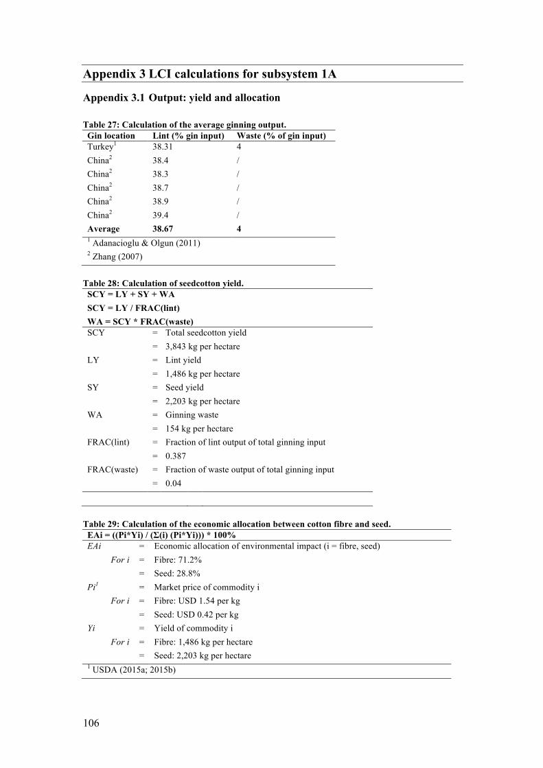
106
Appendix 3 LCI calculations for subsystem 1A
Appendix 3.1 Output: yield and allocation
Table 27: Calculation of the average ginning output. Gin location Lint (% gin input) Waste (% of gin input) Turkey1 38.31 4 China2 38.4 / China2 38.3 / China2 38.7 / China2 38.9 / China2 39.4 / Average 38.67 4 1 Adanacioglu & Olgun (2011) 2 Zhang (2007)
Table 28: Calculation of seedcotton yield. SCY = LY + SY + WA SCY = LY / FRAC(lint) WA = SCY * FRAC(waste) SCY = Total seedcotton yield = 3,843 kg per hectare LY = Lint yield = 1,486 kg per hectare SY = Seed yield = 2,203 kg per hectare WA = Ginning waste = 154 kg per hectare FRAC(lint) = Fraction of lint output of total ginning input = 0.387 FRAC(waste) = Fraction of waste output of total ginning input = 0.04
Table 29: Calculation of the economic allocation between cotton fibre and seed. EAi = ((Pi*Yi) / (Σ(i) (Pi*Yi))) * 100% EAi = Economic allocation of environmental impact (i = fibre, seed)
For i = Fibre: 71.2% = Seed: 28.8% Pi1 = Market price of commodity i
For i = Fibre: USD 1.54 per kg = Seed: USD 0.42 per kg Yi = Yield of commodity i
For i = Fibre: 1,486 kg per hectare = Seed: 2,203 kg per hectare 1 USDA (2015a; 2015b)

107
Appendix 3.2 Input: pesticides
Table 30: Calculation of the pesticide use in cotton cultivation. Product (kg ha-1) Bevilacqua et al. (2014) USDA (2006) Average Parathion (OP) 0.50 0 0.25 Malathion (OP) 0 4.3 2.15 Aldicarb (C) 0 0.75 0.38 Pyrethroid (P) 0.50 0 0.25 Acephate (OP) 0 0.96 0.48 Organophosphorus (OP) 0.50 0 0.25 Trifluralin (DNA) 0 1.01 0.50 Fluormetron (PU) 0.94 0 0.47 Glyphosate 0.91 1.78 1.35 Prometryn (T) 0.74 0.89 0.82 Total active ingredient 4.07 9.70 6.89 OP = organophosphates, C = carbamates, P = pyrethroids, DNA = dinitroaniline, PU = phenylurea, T = triazine
Appendix 3.3 Input: fertilizers
Table 31: Calculation of the fertilizer input in cotton cultivation. TFi = FY * (FEi/YE) TFi = Total amount of fertilizer (i = urea, N-compound, P2O5-compound, K2O-
compound) for i = Kg per hectare GAP scenario CP scenario*
Urea-N: 106 168 N-compound: 85 135 P2O5-compound: 85 85 K2O-compound: 85 85 FY = Fibre yield = 1,486 kg per hectare FEi1 = Good agricultural practice fertilizer use in experiment
for i = Urea-N: 101 kg per hectare N-compound: 81 kg per hectare P2O5-compound: 81 kg per hectare K2O-compound: 81 kg per hectare YE1 = Yield of cotton lint in experiment = 1,430 kg per hectare * For the CP scenario the same amounts are assumed as the GAP scenario but with a total N-application of 303 kg ha-1 instead of 191 kg ha-1 (Lemon et al. 2009; Bevilacqua et al. 2014; Dai & Dong 2014) 1 Dai et al. (2014)

108
Appendix 3.4 Input: irrigation
Table 32: Comparison of the YRR climate with that of southeastern US cotton-growing regions. Location Rain2 (mm) Temperature2 (°C) (% production1) May-Oct May June July August Sept Oct Shaanxi (3.2) 446 20.5 25.6 27.6 26.1 20.4 14.8 Shanxi (4.3) 359 18.3 22.4 24.8 22.8 17.4 10.5 Henan (18.6) 503 21.6 26.8 28.2 26.4 21.6 15.8 Hebei (31.9) 458 20.9 25.7 26.9 25.4 20.6 14.1 Shandong (38.3) 537 21.9 26.5 27.7 26.5 21.9 15.9 Tianjin (3.7) 494 19.9 24.4 26.5 25.7 20.9 14.1 YRR weighted average 493.4 21.3 26.0 27.3 25.9 21.2 15.0 Memphis, Tennessee 548 21.3 25.6 27.4 26.4 22.8 16.9 Montgomery, Alabama 593 22.3 26.0 27.3 26.9 24.3 18.2 1 Barnes et al. (2012) 2 Climate data (2014)
Table 33: Calculation of the minimum irrigation used in YRR cotton cultivation. IR = ((ET-RF) / FFE) * A IR = Total amount of irrigation = 1,512 m3 per hectare ET1 = Evapotranspiration of cotton in warm and humid climate = 637 mm RF = Average rainfall during the cotton growing season = 493 mm FFE2 = Factor incorporating efficiency of Flood-and-furrow
irrigation = 0.4 A3 = Percentage of cotton area irrigated in YRR = 0.42 1 Suleiman et al. (2007) & Perry et al. (2012) 2 Bevilacqua et al. (2014) 3 Barnes et al. (2012)
Appendix 3.5 Input: seed
Table 34: Calculation of the average seed use in cotton cultivation. Source Amount seed (kg ha-1) Average (kg ha-1) Dai & Dong (2014) 35-45 40 Barnes et al. (2012) 15-30 22.5 Personal communication Tian Changyan 45 45 Total 35.8

109
Appendix 3.6 Input: plastic mulch
Table 35: Calculation of the low-density polyethylene film used in cotton production. LDPE = A * TH * D(LDPE) * MF LDPE = Total amount of low density polyethylene film used = 41.3 kg per hectare A1 = Area per hectare covered in plastic mulch = 8,000 m2 TH2 = Average thickness of LPDE film = 8 µm D(LDPE)3 = Density of low density polyethylene film = 922 kg per m3 MF2 = Mulching factor that corrects for farmers not using the
technique = 0.7 1 Zhou et al. (2012) 2 Dai & Dong (2014) 3 Exxon Mobil (2014)
Appendix 3.7 Input: on-farm fuel use
Table 36: Calculation of the total average mechanization in YRR. TAM = Mean(AWA(tillage) + AWA(sowing)) Province of YRR Production (%) Mechanization percentage
Tillage (%) Sowing (%) Shaanxi 3.2 88 34 Shanxi 4.3 100 88 Henan 18.6 25 0.5 Hebei 31.9 100 98 Shandong 38.3 88 69 Area-weighted averages (AWA) 80.2 57.9 Total average mechanization (TAM) 69.05 Source: Dai & Dong (2014)
Table 37: Comparison of a hand tractor with a normal tractor. Factor Hand tractor (HT)1 Tractor (T)2 Ratio HT/T Weight (kg) 318 3,000 0.106 Power (HP) 8.8 80 0.110 Fuel consumption (l h-1) 2.04 16 0.127 Mean ratio 0.117 1 Tractordata (2014) 2 Turunen & van der Werf (2006)

110
Table 38: Calculation of on-farm fuel use in cotton cultivation. FU = Σ(i) (Ni * Ti * HFU * TAM) Ti = Area/width*V FU = Total fuel use = 93.3 l per hectare Ni = Number of application of operation i Ti = Time needed per operation i Operation (i)1 N1 Area (m2)* Width (m)** T (h) Tillage 2 10,000 0.5 8 Intertillage 7 5,000 0.5 4 Sowing 1 10,000 0.5 8 Fertilizing 3 10,000 1 4 Mulching 1 5,600 1 2.24 HFU2 = Average hourly fuel use = 2.04 l per hour TAM = Total average mechanization in YRR = 0.69 * The application area of intertillage is assumed at half a hectare because this happens in between the rows of cotton. The area for mulching is calculated from the area per hectare that is actually mulched (See Dai & Dong (2014)). ** The width is an estimate from the width of a hand tractor and plough (Tractordata 2014). Fertilizer is assumed to have a wider spraying range and mulching plastic is assumed at a width of 1 meter. 1 Dai & Dong (2014) 2 Tractordata (2014)
Appendix 3.8 Input: Ginning
Table 39: Calculation of the electricity consumption in cotton ginning. ECgin = AEC * FY
ECgin = Electricity consumption of ginning = 2095 MJ per hectare
AEC = Average electricity consumption of gins = Australia1: 0.86 MJ per kg
= US2: 1.69 MJ per kg = US3: 1.68 MJ per kg = Average: 1.41 MJ per kg FY = Fibre yield = 1,486 kg per hectare 1 Ismail et al. (2011) 2 Reed & Barnes (2009) 3 Barnes et al. (2012)

111
Table 40: Calculation of the gas consumption in cotton ginning. GCgin = AGC * FY
GCgin = Gas consumption of ginning = 681 MJ per hectare
AGC = Average gas consumption of 6 Australian gins = 0.459 MJ per kg FY = Fibre yield = 1,486 kg per hectare 1 Ismail et al. (2011)
Appendix 3.9 Output: fertilizer emissions
Table 41: Calculation of the NMVOC emissions from cotton cultivation. NMVOC = FE(NMVOC) NMVOC = Emissions of non-methane volatile organic compounds = 0.86 kg per hectare FE(NMVOC) = Fixed emission of NMVOC = 0.86 kg per hectare 1 Hutchings et al. (2013)
Table 42: Calculation of the ammonia emissions from cotton cultivation. NH3 = (((EF(urea1)*N(urea)) + (EF(com)*N(com))) * F(pH)) * (1-EF(N2O1))
NH3 = Emissions of ammonia GAP CP = 28.48 kg per hectare 45.32 kg per hectare EF(urea1)1 = Emission factor for ammonia from urea fertilizer (pH-independent) = 0.243 kg NH3 per kg N from urea fertilizer N(urea) = Amount of N applied per hectare from urea fertilizer GAP CP = 105.5 kg per hectare 167.9 kg per hectare EF(com)1 = Emission factor for ammonia from compound fertilizer (pH-independent) = 0.037 kg NH3 per kg N from compound fertilizer N(com) = Amount of N applied per hectare from compound fertilizer GAP CP = 84.7 kg per hectare 135.2 kg per hectare F(pH)1 = pH-dependent factor from the tier 2 model = 1 (because both EFs are pH-independent) EF(N2O1)2 = Emission factor for indirect nitrous oxides from ammonia emissions = 0.01 1 Hutchings et al. (2013) 2 De Klein et al. (2006)

112
Table 43: Calculation of the nitric oxides emissions from cotton cultivation. NOx = (EF(tot1)*N(tot)) * (1-EF(N2O2)) NOx = Emissions of nitrogen oxides GAP CP = 10.49 kg per hectare 16.66 kg per hectare EF(tot1)1 = Emission factor for nitrogen oxides from total nitrogen fertilizer = 0.026 kg NOx per kg N from fertilizer N(tot) = Amount of N applied per hectare from all nitrogen fertilizer GAP CP = 190.2 kg per hectare 303.1 kg per hectare EF(N2O2)2 = Emission factor for indirect nitrous oxides from nitrogen oxide emissions = 0.01 1 Hutchings et al. (2013)
2 De Klein et al. (2006) Table 44: Calculation of the nitrate emissions from cotton cultivation. NO3 = ((EF(tot3)*N(tot)) * (1-EF(N2O3))) * W(NO3) NO3 = Leached nitrate emissions GAP CP = 250.81 kg per hectare 398.22 kg per hectare EF(tot3)1 = Emission factor for nitrates from total nitrogen fertilizer = 0.3 kg NO3-N per kg N from fertilizer N(tot) = Amount of N applied per hectare from all nitrogen fertilizer GAP CP = 190.2 kg per hectare 303.1 kg per hectare EF(N2O3)2 = Emission factor for indirect nitrous oxides from leached nitrates = 0.0075 kg N2O-N per kg N from NO3 emissions W(NO3) = Factor for multiplying NO3-N weight to NO3 weight = 62/14 1 Mosier et al. (1998) 2 De Klein et al. (2006)

113
Table 45: Calculation of the nitrous oxide emissions from cotton cultivation. N2O = N2O(direct) + N2O(indirect) N2O(direct) = (EF(tot2)*N(tot)) * W(N2O) N2O(indirect) = (EF(N2O1)*N(NH3)) + (EF(N2O2)*N(NOx)) + (EF(N2O3)*N(NO3)) N2O = Total emissions of nitrous oxides GAP CP = 4.11 kg per hectare 6.48 kg per hectare N2O(direct) = Direct nitrous oxide emissions GAP CP = 2.99 kg per hectare 4.76 kg per hectare N2O(indirect) = Indirect nitrous oxide emissions GAP CP = 1.12 kg per hectare 1.72 kg per hectare EF(tot2)1 = Emission factor for nitrous oxides from total nitrogen fertilizer = 0.01 kg N2O-N per kg N from fertilizer N(tot) = Amount of N applied per hectare from all nitrogen fertilizer = 190.2 kg per hectare W(N2O) = Factor for multiplying N2O-N weight to N2O weight = 44/28 EF(N2O1)1 = Emission factor for indirect nitrous oxides from ammonia emissions = 0.01 kg N2O-N per kg N from NH3 emissions N(NH3) = Amount of nitrogen in NH3 emissions = NH3/(17/14) GAP CP = 23.69 kg per hectare 37.70 kg per hectare EF(N2O2)1 = Emission factor for indirect nitrous oxides from nitrogen oxide emissions = 0.01 kg N2O-N per kg N from NOx emissions N(NOx) = Amount of nitrogen in NOx emissions = NOx/(30/14)* GAP CP = 4.95 kg per hectare 7.85 kg per hectare EF(N2O3)1 = Emission factor for indirect nitrous oxides from leached nitrates = 0.0075 kg N2O-N per kg N from NO3 emissions N(NOx) = Amount of nitrogen in leached NO3 = NO3/(62/14) GAP CP = 57.06 kg per hectare 90.60 kg per hectare * For weight only NO is assumed. 1 De Klein et al. (2006)

114
Table 46: Calculation of the phosphate emissions from cotton cultivation. PO4 = PO4(leach) + PO4(runoff) PO4(leach) = FE(PO4) * W(PO4) PO4(runoff) = (AF * (1+(0.0025*P(tot)))) * W(PO4) PO4 = Total phosphate emissions = 0.86 kg per hectare PO4(leach) = Phosphate emissions from leaching = 0.21 kg per hectare PO4(runoff) = Phosphate emissions from field runoff = 0.65 kg per hectare FE(PO4)1 = Fixed emission estimate for arable land = 0.07 kg PO4-P per hectare W(PO4) = Factor for multiplying PO4-P weight to PO4 weight = 95/31 AC1 = Arable land constant = 0.175 kg PO4-P per hectare P(tot) = Amount of P2O5 applied per hectare from all phosporus fertilizer = 84.7 kg per hectare 1 Nemecek (2013)
Table 47: Calculation of the carbon dioxide emissions from cotton cultivation. CO2 = EF(urea2) * N(urea) * W(CO2) CO2 = Emission of CO2 from urea fertilizer GAP CP = 165.8 kg per hectare 264.9 kg per hectare EF(urea2)1 = Emission factor of carbon from urea fertilizer = 0.43 kg CO2-C per kg of urea-N N(urea) = Amount of N applied per hectare from urea fertilizer GAP CP = 105.5 kg per hectare 167.9 kg per hectare W(CO2) = Factor for multiplying CO2-C weight to CO2 weight = 44/12 1 De Klein et al. (2006)

115
Table 48: Calculation of the heavy metal emissions from cotton cultivation. HMi = HMi(fert) - HMi(cot) HMi(fert) = Σ(j) (MCji*TOTj) HMi(cot) = ((MCFi*FY) + (MCSi*SY)) HMi = Net heavy metal i emission to soil (i = Cd, Cu, Zn, Pb, Ni, Cr)
GAP CP For i = Cd: 4.2 g per ha 4.2 g per ha
Cu: 5.8 g per ha 8.4 g per ha Zn: 37.5 g per ha 51.2 g per ha Pb: 1.1 g per ha 1.7 g per ha Ni: 3.4 g per ha 5.3 g per ha Cr: 56.2 g per ha 57.1 g per ha HMi(fert) = Amount of heavy metal i added to the soil by fertilizers MCji1 = Mean content of heavy metal i (mg per kg j) in j-fertilizer (j = N, P2O5,
K2O) = i/j N P2O5 K2O Cd 0.21 51.32 0.11 Cu 22.25 118.22 6.17 Zn 121.43 751.32 70.33 Pb 5.37 49.42 7.88 Ni 17.17 100.46 7.52 Cr 7.81 589.46 88.54 TOTj = Total amount of j-fertilizer
GAP CP For j = N: 190.2 kg per ha 303.1 kg per ha
P2O5: 84.7 kg per ha 84.7 kg per ha K2O: 84.7 kg per ha 84.7 kg per ha HMi(cot) = Amount of heavy metal i accumulated in cotton fibre and seed MCFi/MCSi1,2 = Mean content for metal I in cotton fibre and cotton seed = Fibre
(mg kg-1) Seed (mg kg-1)
Cd 0.07 0.05 Cu 1.1 3.3 Zn 11.5 17.3 Pb 2.5 0.5 Ni* 2.44 Cr* 0.73 FY/SY = Fibre/seed yield = 1,486/2,203 kg per ha * Specific values for cotton are only available for Cd, Cu, Zn and Pb (Angelova et al. 2004). Estimates for Ni and Cr were made by averaging heavy metal contents of grass, potatoes and soybeans as reported by Freiermuth (2006). These averages for Cd, Cu, Zn and Pb were in the correct order of magnitude so the estimate is assumed as solid. 1 Freiermuth (2006) 2 Angelova et al. (2004)

116
Appendix 3.10 Output: pesticide emissions
Table 49: Comparison of assumed environmental fates of pesticides in cotton cultivation. Pesticide emissions Vapor pressure
(mPa) Fraction to air
Soil mobility
Fraction to soil4
Solubility (g l-1)
Fraction to water
Parathion1 5 0.50 none 0.50 negligible 0 Malathion2 16.6 0.95 high 0 0.145 0.05 Aldicarb1 10 0.50 high 0 9 0.50 Pyrethroid2 low 0.01 none 0.99 negligible 0 Acephate2 2.3 0.50 high 0 790 0.50 Organophosporus3 / 0.50 high 0.50 / 0 Trifluralin1 15 0.95 none 0.05 0.0024 0 Fluormeturon1 0.066 0.05 high 0 0.1 0.95 Glyphosate2 negligible 0.05 none 0.95 10 0 Prometryn1 0.16 0.15 low 0.85 0.033 0 1 PMEP (2015) 2 NPIC (2015) 3 PIO (2015) 4 Webb et al. (2013)
Table 50: Calculation of the pesticide emissions from cotton cultivation. Emissions Air (kg ha-1) Water (kg ha-1) Soil (kg ha-1) Parathion 0.125 0 0.125 Malathion 2.0425 0.1075 0 Aldicarb 0.19 0.19 0 Pyrethroid 0.0025 0 0.2475 Acephate 0.24 0.24 0 Organophosporus 0.125 0 0.125 Trifluralin 0.475 0 0.025 Fluormeturon 0.0235 0.4465 0 Glyphosate 0.0675 0 1.2825 Prometryn 0.123 0 0.697
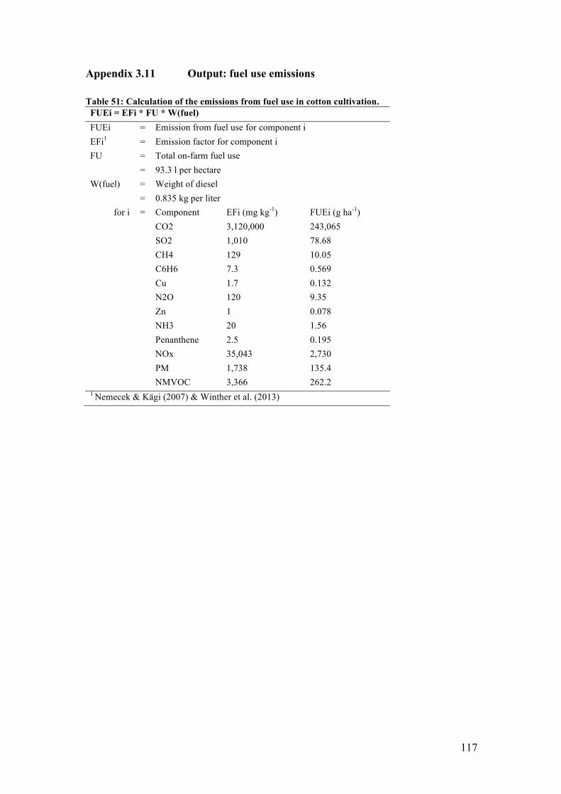
117
Appendix 3.11 Output: fuel use emissions
Table 51: Calculation of the emissions from fuel use in cotton cultivation. FUEi = EFi * FU * W(fuel) FUEi = Emission from fuel use for component i EFi1 = Emission factor for component i FU = Total on-farm fuel use = 93.3 l per hectare W(fuel) = Weight of diesel = 0.835 kg per liter
for i = Component EFi (mg kg-1) FUEi (g ha-1) CO2 3,120,000 243,065 SO2 1,010 78.68 CH4 129 10.05 C6H6 7.3 0.569 Cu 1.7 0.132 N2O 120 9.35 Zn 1 0.078 NH3 20 1.56 Penanthene 2.5 0.195 NOx 35,043 2,730 PM 1,738 135.4 NMVOC 3,366 262.2 1 Nemecek & Kägi (2007) & Winther et al. (2013)

118
Appendix 4 LCI calculations for subsystem 1B
Appendix 4.1 Output: yield and allocation
Table 52: Comparison of hemp yields with distribution of fibre and shivs. Source Location Total stem yield
(t DM ha-1) Fibre content (%)
Shivs content (%)
Amaducci et al. (2014) China 6.6 - 10.9 / / Clarke 1(995) China 8 - 12 / / Zheng et al. (2013) China / 22.3 / Barth & Carus (2015) Europe 7 - 9 28 55 Assumed Heilongjiang 10 22 55
Table 53: Calculation of hemp yield in Heilongjiang province. FY = TSY - RL - SY - SW
FY = Fibre yield after scutching = 2,200 kg per hectare TSY = Total stem yield before retting and scutching = 10,000 kg per hectare RL1 = Retting loss of stem biomass = 0.1 * TSY = 1,000 kg per hectare SY = Shivs yield after scutching = 5,500 kg per hectare SW = Scutching waste = 1,300 kg per hectare 1 Turunen & van der Werf (2006)
Table 54: Calculation of the economic allocation between hemp fibre and shivs. EAi = ((Pi * Yi) / (Σ(i) (Pi * Yi))) * 100%
EAi = Economic allocation of environmental impact (i = fibre, seed) For i = Fibre: 52.8%
= Shivs: 47.2% Pi1 = Market price of commodity i
For i = Fibre: EUR 0.70 per kg = Shivs: EUR 0.25 per kg Yi = Yield of commodity i
For i = Fibre: 2,200 kg per hectare = Shivs: 5,500 kg per hectare 1 Personal communication Martha Barth (March 27th 2015)

119
Appendix 4.2 Input: pesticides
Table 55: Calculation of the pesticide use in hemp cultivation. AI = AR * C * D AI = Total amount of active ingredient metolachlor = 2,145 g per hectare AR1 = Application rate = 3 L per hectare C1 = Concentration of emulsion = 65% metolachlor per liter D2 = Density of metolachlor = 1.1 kg per liter 1 Amaducci et al. (2014) 2 NPIC (2015)
Appendix 4.3 Input: fertilizer
Table 56: Comparison of the fertilizer input in GAP and CP hemp cultivation scenarios. Scenario Urea-N (kg ha-1) P2O5 (kg ha-1) K2O (kg ha-1)
GAP1 90 100 80 CP2 200 75 150 1 Song et al. (2012) 2 Liu (2013)
Appendix 4.4 Input: seeds
Table 57: Calculation of the seed used in hemp cultivation. IS = (SR / SY) * IHH IS = Impact of seed = 0.0485*IHH SR1 = Seed rate of fibre hemp = 80 kg per hectare SY2 = Average seed yield in China = 1,650 kg per hectare IHH = Impact hectare hemp production = Fertilizer, pesticide, fuel use and emissions from LCI 1 Liu (2013) 2 Yunnan Industrial Hemp (2015)

120
Appendix 4.5 Input: on-farm fuel use
Table 58: Calculation of the on-farm fuel use in hemp cultivation. FU = Σ(i) (Ni * Ti * HFU * TAM) Ti = Area/width*V FU = Total fuel use = 69.4 l per hectare Ni = Number of application of operation i Ti = Time needed per operation i Operation1 N Area (m2)* width (m)** T (h) Tillage 2 10,000 0.5 8 Sowing 1 10,000 0.5 8 Fertilizing/
pesticide 3 10,000 1 4
Harvesting 1 10,000 1 2.24 HFU2 = Average hourly fuel use = 2.04 l per hour TAM = Total average mechanization in Heilongjiang = 0.85 * As opposed to cotton, all operations are applied to the entire field area. ** The with is an estimate from the width of a hand tractor and plough (Tractordata 2014). Fertilizing and pesticide application is assumed to have a wider spraying range. 1 Liu (2013) 2 Tractordata (2014)
Appendix 4.6 Input: scutching
Table 59: Calculation of the electricity consumption of hemp scutching. ECscutch = AEC * FY
ECgin = Electricity consumption of scutching = 3,146 MJ per hectare
AEC = Average electricity consumption of scutching machines = Hungary1: 1.65 MJ per kg
= Spain2: 1.21 MJ per kg = Average: 1.43 MJ per kg FY = Fibre yield = 2,200 kg per hectare 1 Turunen & van der Werf (2006) 2 González-García et al. (2010)

121
Appendix 4.7 Output: fertilizer emissions
Table 60: Calculation of the NMVOC emissions from hemp cultivation. NMVOC = FE(NMVOC) NMVOC = Emissions of non-methane volatile organic compounds = 0.86 kg per hectare FE(NMVOC) = Fixed emission of NMVOC = 0.86 kg per hectare 1 Hutchings et al. (2013)
Table 61: Calculation of the ammonia emissions from hemp cultivation. NH3 = (((EF(urea1)*N(urea)) + (EF(com)*N(com))) * F(pH)) * (1-EF(N2O1))
NH3 = Emissions of ammonia GAP CP = 21.87 kg per hectare 48.11 kg per hectare EF(urea1)1 = Emission factor for ammonia from urea fertilizer (pH-independent) = 0.243 kg NH3 per kg N from urea fertilizer N(urea) = Amount of N applied per hectare from urea fertilizer GAP CP = 90 kg per hectare 200 kg per hectare EF(com)1 = Emission factor for ammonia from compound fertilizer (pH-independent) = 0.037 kg NH3 per kg N from compound fertilizer N(com) = Amount of N applied per hectare from compound fertilizer = 0 kg per ha F(pH)1 = pH-dependent factor from the tier 2 model = 1 (because both EFs are pH-independent) EF(N2O1)2 = Emission factor for indirect nitrous oxides from ammonia emissions = 0.01 1 Hutchings et al. (2013) 2 De Klein et al. (2006)
Table 62: Calculation of the nitric oxides emissions from hemp cultivation. NOx = (EF(tot1)*N(tot)) * (1-EF(N2O2)) NOx = Emissions of nitrogen oxides GAP CP = 4.96 kg per hectare 11.03 kg per hectare EF(tot1)1 = Emission factor for nitrogen oxides from total nitrogen fertilizer = 0.026 kg NOx per kg N from fertilizer N(tot) = Amount of N applied per hectare from all nitrogen fertilizer GAP CP = 90 kg per hectare 200 kg per hectare EF(N2O2)2 = Emission factor for indirect nitrous oxides from nitrogen oxide emissions = 0.01 1 Hutchings et al. (2013)
2 De Klein et al. (2006)

122
Table 63: Calculation of the nitrous oxide emissions from hemp cultivation. N2O = N2O(direct) + N2O(indirect) N2O(direct) = (EF(tot2)*N(tot)) * W(N2O) N2O(indirect) = (EF(N2O1)*N(NH3)) + (EF(N2O2)*N(NOx)) + (EF(N2O3)*N(NO3)) N2O = Total emissions of nitrous oxides GAP CP = 2.05 kg per hectare 4.56 kg per hectare N2O(direct) = Direct nitrous oxide emissions GAP CP = 1.41 kg per hectare 3.14 kg per hectare N2O(indirect) = Indirect nitrous oxide emissions GAP CP = 0.64 kg per hectare 1.42 kg per hectare EF(tot2)1 = Emission factor for nitrous oxides from total nitrogen fertilizer = 0.01 kg N2O-N per kg N from fertilizer N(tot) = Amount of N applied per hectare from all nitrogen fertilizer = 190.2 kg per hectare W(N2O) = Factor for multiplying N2O-N weight to N2O weight = 44/28 EF(N2O1)1 = Emission factor for indirect nitrous oxides from ammonia emissions = 0.01 kg N2O-N per kg N from NH3 emissions N(NH3) = Amount of nitrogen in NH3 emissions = NH3/(17/14) GAP CP = 18.01 kg per hectare 40.02 kg per hectare EF(N2O2)1 = Emission factor for indirect nitrous oxides from nitrogen oxide emissions = 0.01 kg N2O-N per kg N from NOx emissions N(NOx) = Amount of nitrogen in NOx emissions = NOx/(30/14)* GAP CP = 2.34 kg per hectare 5.20 kg per hectare EF(N2O3)1 = Emission factor for indirect nitrous oxides from leached nitrates = 0.0075 kg N2O-N per kg N from NO3 emissions N(NOx) = Amount of nitrogen in leached NO3 = NO3/(62/14) GAP CP = 27.00 kg per hectare 59.55 kg per hectare * For weight only NO is assumed. 1 De Klein et al. (2006)

123
Table 64: Calculation of the nitrate emissions from hemp cultivation. NO3 = ((EF(tot3)*N(tot)) * (1-EF(N2O3))) * W(NO3) NO3 = Leached nitrate emissions GAP CP = 118.67 kg per hectare 263.72 kg per hectare EF(tot3)1 = Emission factor for nitrates from total nitrogen fertilizer = 0.3 kg NO3-N per kg N from fertilizer N(tot) = Amount of N applied per hectare from all nitrogen fertilizer GAP CP = 90 kg per hectare 200 kg per hectare EF(N2O3)2 = Emission factor for indirect nitrous oxides from leached nitrates = 0.0075 kg N2O-N per kg N from NO3 emissions W(NO3) = Factor for multiplying NO3-N weight to NO3 weight = 62/14 1 Mosier et al. (1998) 2 De Klein et al. (2006)
Table 65: Calculation of the phosphate emissions from hemp cultivation. PO4 = PO4(leach) + PO4(runoff) PO4(leach) = FE(PO4) * W(PO4) PO4(runoff) = (AF * (1+(0.0025*P(tot)))) * W(PO4) PO4 = Total phosphate emissions GAP CP = 0.88 kg per hectare 0.85 kg per hectare PO4(leach) = Phosphate emissions from leaching GAP CP = 0.21 kg per hectare 0.21 kg per hectare PO4(runoff) = Phosphate emissions from field runoff GAP CP = 0.67 kg per hectare 0.64 FE(PO4)1 = Fixed emission estimate for arable land = 0.07 kg PO4-P per hectare W(PO4) = Factor for multiplying PO4-P weight to PO4 weight = 95/31 AC1 = Arable land constant = 0.175 kg PO4-P per hectare P(tot) = Amount of P2O5 applied per hectare from all phosporus fertilizer GAP CP = 100 kg per hectare 75 kg per hectare 1 Nemecek (2013)

124
Table 66: Calculation of the carbon dioxide emissions from hemp cultivation. CO2 = EF(urea2) * N(urea) * W(CO2) CO2 = Emission of CO2 from urea fertilizer GAP CP = 141.9 kg per hectare 315.3 kg per hectare EF(urea2)1 = Emission factor of carbon from urea fertilizer = 0.43 kg CO2-C per kg of urea-N N(urea) = Amount of N applied per hectare from urea fertilizer GAP CP = 90 kg per hectare 200 kg per hectare W(CO2) = Factor for multiplying CO2-C weight to CO2 weight = 44/12 1 De Klein et al. (2006)

125
Table 67: Calculation of the heavy metal emissions from hemp cultivation. HMi = HMi(fert) - HMi(cot) HMi(fert) = Σ(j) (MCji * TOTj) HMi(cot) = ((MCFi*FY) + (MCSi*SY)) HMi = Net heavy metal i emission to soil (i = Cd, Cu, Zn, Pb, Ni, Cr)
GAP CP For i = Cd: 2.3 g per ha 1 g per ha
Cu: -14.3 g per ha -14.4 g per ha Zn: -10.2 g per ha -10.7 g per ha Pb: -17.3 g per ha -17.4 g per ha Ni: -12.2 g per ha -12.3 g per ha Cr: 59.4 g per ha 51.8 g per ha HMi(fert) = Amount of heavy metal i added to the soil by fertilizers MCji1 = Mean content of heavy metal i (mg per kg j) in j-fertilizer (j = N, P2O5,
K2O) = i/j N P2O5 K2O Cd 0.21 51.32 0.11 Cu 22.25 118.22 6.17 Zn 121.43 751.32 70.33 Pb 5.37 49.42 7.88 Ni 17.17 100.46 7.52 Cr 7.81 589.46 88.54 TOTj = Total amount of j-fertilizer
GAP CP For j = N: 90 kg per ha 200 kg per ha
P2O5: 100 kg per ha 75 kg per ha K2O: 80 kg per ha 150 kg per ha HMi(cot) = Amount of heavy metal i accumulated in hemp fibre and residual stem MCFi/MCSi1,2 = Mean content for metal I in hemp fibre and residual stem = Fibre
(mg kg-1) Stems (mg kg-1)
Cd 0.15 0.33 Cu 1.3 3.3 Zn 1.3 12.7 Pb 2.1 2.4 Ni* 2.44 Cr* 0.73 FY/SY = Fibre/residual stem yield = 2,200/7,800 kg per ha * Specific values for cotton are only available for Cd, Cu, Zn and Pb (Angelova et al. 2004). Estimates for Ni and Cr were made by averaging heavy metal contents of grass, potatoes and soybeans as reported by Freiermuth (2006). These averages for Cd, Cu, Zn and Pb were in the correct order of magnitude so the estimate is assumed as solid. 1 Freiermuth (2006) 2 Angelova et al. (2004)
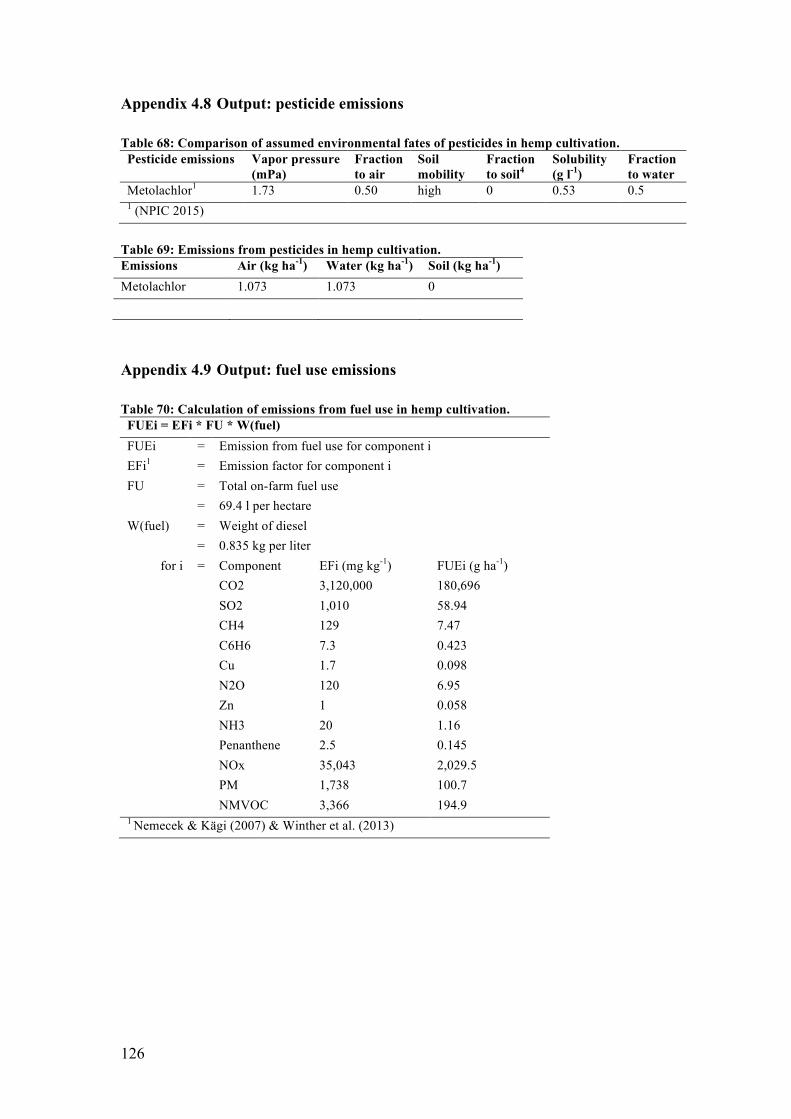
126
Appendix 4.8 Output: pesticide emissions
Table 68: Comparison of assumed environmental fates of pesticides in hemp cultivation. Pesticide emissions Vapor pressure
(mPa) Fraction to air
Soil mobility
Fraction to soil4
Solubility (g l-1)
Fraction to water
Metolachlor1 1.73 0.50 high 0 0.53 0.5 1 (NPIC 2015)
Table 69: Emissions from pesticides in hemp cultivation. Emissions Air (kg ha-1) Water (kg ha-1) Soil (kg ha-1) Metolachlor 1.073 1.073 0
Appendix 4.9 Output: fuel use emissions
Table 70: Calculation of emissions from fuel use in hemp cultivation. FUEi = EFi * FU * W(fuel) FUEi = Emission from fuel use for component i EFi1 = Emission factor for component i FU = Total on-farm fuel use = 69.4 l per hectare W(fuel) = Weight of diesel = 0.835 kg per liter
for i = Component EFi (mg kg-1) FUEi (g ha-1) CO2 3,120,000 180,696 SO2 1,010 58.94 CH4 129 7.47 C6H6 7.3 0.423 Cu 1.7 0.098 N2O 120 6.95 Zn 1 0.058 NH3 20 1.16 Penanthene 2.5 0.145 NOx 35,043 2,029.5 PM 1,738 100.7 NMVOC 3,366 194.9 1 Nemecek & Kägi (2007) & Winther et al. (2013)

127
Appendix 4.10 Output: retting emissions
Table 71: Calculation of the nitrogen emissions from hemp retting. REi = RL * NC * EFi
REi = Emissions from retting (i = N2O, NH3 and NOx) For i = N2O: 448 g per hectare
= NH3: 950 g per hectare = NOx: 988 g per hectare RL = Retting loss of stem biomass = 1,000 kg per hectare NC1 = Average N-content of hemp plant material = 0.0095 kg N per kg hemp stem EFi2,3 = Emission factor for N from decomposing organic matter (most conservative)
For i = N2O: 0.047 kg N2O per kg N = NH3: 0.1 kg NH3 per kg N = NOx: 0.104 kg NOx per kg N
1 Liu (2013) 2 De Klein et al. (2006) 3 Hutchings et al. (2013)

128
Appendix 5 LCI of subsystem 1A and 1B
Appendix 5.1 LCI of subsystem 1A: Cotton scenario
Table 72: LCI of two scenarios for one hectare cotton production. Type Category Compound Quantity*: GAP CP Unit Comp.** Ouptut Product Ginned cotton lint 1,486 kg Output By-product Ginned cottonseed 2,203 kg Output Waste Ginning waste 154 kg Waste Input Insecticide Parathion (OP) 0.25 kg Input Insecticide Malathion (OP) 2.15 kg Input Insecticide Aldicarb (C) 0.38 kg Input Insecticide Pyrethroid (P) 0.25 kg Input Insecticide Acephate (OP) 0.48 kg Input Insecticide Organophosphorus (OP) 0.25 kg Input Herbicide Trifluralin (DNA) 0.50 kg Input Herbicide Fluormetron (PU) 0.47 kg Input Herbicide Glyphosate 1.35 kg Input Herbicide Prometryn (T) 0.82 kg Input Fertilizer N from ammonium in compound fertilizer 84.7 133.7 kg Input Fertilizer N from urea fertilizer 105.5 167.8 kg Input Fertilizer P2O5 from compound fertilizer 84.7 84.7 kg Input Fertilizer K2O from compound fertilizer 84.7 84.7 kg Input Irrigation Pumping of irrigation water 1,512 m3 Input Seed Cotton seed for sowing 35.8 kg Input Mulching Low-density polyethylene mulch 41.3 kg Input Fuel use On-farm fuel use 93.3 l Input Ginning Electricity consumption 2,095.3 MJ Input Ginning Heating energy from natural gas 681.5 MJ Output Fertilizer Non-methane volatile organic compounds 0.86 0.86 kg Air Output Fertilizer Ammonia 28.48 45.32 kg Air Output Fertilizer Nitrogen oxides 10.49 16.66 kg Air Output Fertilizer Nitrous oxides 4.11 6.48 kg Air Output Fertilizer Nitrates 250.81 398.22 kg Water Output Fertilizer Phosphates 0.86 0.86 kg Water Output Fertilizer Carbon dioxide 165.80 264.88 kg Air Output Fertilizer Cadmium 4.2 4.2 g Soil Output Fertilizer Copper 6.0 8.4 g Soil Output Fertilizer Zinc 37.5 51.2 g Soil Output Fertilizer Lead 1.0 1.7 g Soil Output Fertilizer Nickel 3.4 5.3 g Soil Output Fertilizer Chrome 56.2 57.1 g Soil Output Insecticide Parathion (OP) 125 g Air Output Insecticide Parathion (OP) 125 g Soil Output Insecticide Malathion (OP) 2,043 g Air Output Insecticide Malathion (OP) 108 g Water Output Insecticide Aldicarb (C) 190 g Air Output Insecticide Aldicarb (C) 190 g Water Output Insecticide Pyrethroid (P) 2.5 g Air Output Insecticide Pyrethroid (P) 248 g Soil Output Insecticide Acephate (OP) 240 g Air Output Insecticide Acephate (OP) 240 g Water Output Insecticide Organophosphorus (OP) 125 g Air Output Insecticide Organophosphorus (OP) 125 g Soil Output Herbicide Trifluralin (DNA) 475 g Air Output Herbicide Trifluralin (DNA) 25 g Soil Output Herbicide Fluormeturon (PU) 34 g Air Output Herbicide Fluormeturon (PU) 447 g Water Output Herbicide Glyphosate 68 g Air Output Herbicide Glyphosate 1,283 g Soil Output Herbicide Prometryn (T) 123 g Air Output Herbicide Prometryn (T) 697 g Soil Output Fuel use Carbon dioxide 243.1 kg Air Output Fuel use Sulfur dioxide 78.68 g Air Output Fuel use Methane 10.05 g Air Output Fuel use Benzene 0.569 g Air Output Fuel use Nitrous oxide 9.35 g Air Output Fuel use Zinc 0.078 g Air

129
Output Fuel use Ammonia 1.56 g Air Output Fuel use Penanthene 0.195 g Air Output Fuel use Nitrogens oxids 2,730 g Air Output Fuel use Particulate matter 135.4 g Air Output Fuel use Non-methane volatile organic compounds 262.2 g Air * Table contains LCI before economic allocation between cotton fibre and seed. ** Comp. = Compartment
Appendix 5.2 LCI of subsystem 1B: Hemp scenario
Table 73: LCI of two scenarios for one hectare hemp production. Type Category Compound Quantity*: GAP CP Unit Comp. Ouptut Product Scutched hemp fibre 2,200 kg Output By-product Hemp shivs 5,500 kg Output Waste Scutching waste 1,300 kg Waste Input Herbicide Metolachlor 2.15 kg Input Fertilizer N from urea fertilizer 90 200 kg Input Fertilizer P2O5 from compound fertilizer 100 75 kg Input Fertilizer K2O from compound fertilizer 80 150 kg Input Seed Hemp seed for sowing 80 kg Input Fuel use On-farm fuel use 69.4 l Input Scutching Electricity consumption 3,146 MJ Output Fertilizer Non-methane volatile organic compounds 0.86 0.86 kg Air Output Fertilizer Ammonia 21.65 48.11 kg Air Output Fertilizer Nitrogen oxides 4.96 11.03 kg Air Output Fertilizer Nitrous oxide 2.05 4.56 kg Air Output Fertilizer Nitrates 118.67 263.72 kg Water Output Fertilizer Phosphates 0.88 0.85 kg Water Output Fertilizer Carbon dioxide 141.9 315.3 kg Air Output Fertilizer Cadmium 2.3 1.0 g Soil Output Fertilizer Copper -14.3 -14.4 g Soil Output Fertilizer Zinc -10.2 -10.7 g Soil Output Fertilizer Lead -17.3 -17.4 g Soil Output Fertilizer Nickel -12.2 -12.3 g Soil Output Fertilizer Chrome 59.4 51.8 g Soil Output Herbicide Metolachlor 1,073 g Air Output Herbicide Metolachlor 1,073 g Water Output Fuel use Carbon dioxide 180.7 kg Air Output Fuel use Sulfur dioxide 58.49 g Air Output Fuel use Methane 7.47 g Air Output Fuel use Benzene 0.423 g Air Output Fuel use Nitrous oxide 6.95 g Air Output Fuel use Zinc 0.058 g Air Output Fuel use Ammonia 1.16 g Air Output Fuel use Penanthene 0.145 g Air Output Fuel use Nitrogen oxides 2,029.5 g Air Output Fuel use Particulate matter 100.7 g Air Output Fuel use Non-methane volatile organic compounds 194.9 g Air Output Scutching Nitrous oxide 448 g Air Output Scutching Ammonia 950 g Air Output Scutching Nitrogen oxides 988 g Air * Table contains LCI before economic allocation between hemp fibre and shivs. ** Comp. = Compartment

130
Appendix 6 Data quality assessment
Appendix 6.1 Quality of hemp LCI data
Table 74: Summary of the uncertainty ranking of the data in the hemp LCI.
Phase Data Source Uncertainty
Cul
tivat
ion
Yield Secondary Literature-based estimate
Medium
Economic allocation
Secondary Expert communication
Medium
Pesticide production
Secondary Literature
Low
Fertilizer production
Secondary Literature
Medium
Seed Secondary Literature average
Low
Fuel use Secondary Literature-based estimate
High
Scutching Secondary Literature
Medium
Pesticide emissions
Secondary Literature and expert communication
High
Fertilizer emissions
Secondary Literature
Medium
Fuel emissions
Secondary Literature
Low
Spin
ning
and
wea
ving
Degumming agents
Primary Chinese textile manufacturer1
Medium
Degumming emissions
Secondary Expert communication
High
Energy Primary Chinese textile manufacturer1
High
Material efficiency
Primary Chinese textile manufacturer1
High
Sizing agent Primary Chinese textile manufacturer1
Medium
1 The manufacturer wishes for remain anonymous

131
Appendix 6.2 Quality of cotton LCI data
Table 75: Summary of the uncertainty ranking of the data in the cotton LCI. Phase Data Type Uncertainty
Cul
tivat
ion
Yield Secondary Databases and literature
Low
Economic allocation
Secondary Databases
Low
Pesticide production
Secondary LCI and database
Medium
Fertilizer production
Secondary Literature
Low
Irrigation Secondary Literature-based estimate
Medium
Seed Secondary Literature average
Medium
Mulching Secondary Literature and expert communication
Low
Fuel use Secondary Literature-based estimate
High
Ginning Secondary Literature
Low
Pesticide emissions
Secondary Literature and expert communication
High
Fertilizer emissions
Secondary Literature
Medium
Fuel emissions
Secondary Literature
Low
Spin
ning
an
d w
eavi
ng Energy Secondary
Literature-based estimate High
Material efficiency
Secondary Literature
Low
Sizing agent
Primary Chinese textile manufacturer
Medium
1 The manufacturer wishes for remain anonymous
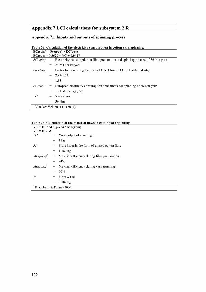
132
Appendix 7 LCI calculations for subsystem 2 R
Appendix 7.1 Inputs and outputs of spinning process
Table 76: Calculation of the electricity consumption in cotton yarn spinning. EC(spin) = F(cn/eu) * EC(eus) EC(eus) = 0.3627 * YC + 0.0427 EC(spin) = Electricity consumption in fibre preparation and spinning process of 36 Nm yarn = 24 MJ per kg yarn F(cn/eu) = Factor for correcting European EU to Chinese EU in textile industry = 2.97/1.62 = 1.83 EC(eus)1 = European electricity consumption benchmark for spinning of 36 Nm yarn = 13.1 MJ per kg yarn YC = Yarn count = 36 Nm 1 Van Der Velden et al. (2014)
Table 77: Calculation of the material flows in cotton yarn spinning. YO = FI * ME(prep) * ME(spin) YO = FI - W YO = Yarn output of spinning = 1 kg FI = Fibre input in the form of ginned cotton fibre = 1.182 kg ME(prep)1 = Material efficiency during fibre preparation = 94% ME(spin)1 = Material efficiency during yarn spinning = 90% W = Fibre waste = 0.182 kg 1 Blackburn & Payne (2004)

133
Appendix 7.2 Outputs of sizing process
Table 78: Calculation of the COD removed in treatment and emitted from cotton sizing. COD(tot) = CODC(st) * SC COD(tot) = COD(treat) + COD(env) COD(tot) = Total COD in wastewater = 90 g per kg yarn CODC(st)1 = COD-content for starch = 1 g per g SC = Starch consumption = 90 g per kg yarn COD(treat)2 = COD removed by treatment = 82.8 g per kg yarn COD(env) = COD not removed and emitted to environment = 7.2 g per kg yarn 1 IPPC (2003) 2 Yuan et al. (2013)
Appendix 7.3 Inputs and outputs of weaving process
Table 79 Calculation of the electricity consumption in cotton fabric weaving. EC(we) = F(cn/eu) * EC(euw) EC(euw) = 0.5328 * YC – 0.0311 EC(we) = Electricity consumption in sizing and weaving process of 36 Nm yarn = 35 MJ per kg fabric F(cn/eu) = Factor for correcting European EU to Chinese EU in textile industry = 1.83 EC(euw)1 = European electricity consumption benchmark for weaving of 36 Nm yarn = 19.1 MJ per kg yarn YC = Yarn count = 36 Nm 1 Van Der Velden et al. (2014)

134
Table 80: Calculation of the material flows in cotton fabric weaving. FO = YI * ME(we) FO = YI(weft) + YI(warp) - W FO = Fabric output of weaving = 1 kg YI(weft) = Yarn input of weft yarn = 0.5 kg per kg fabric YI(warp) = Yarn input of warp yarn = 0.57 kg per kg fabric ME(we)1 = Material efficiency during weaving = 94% W = Fibre waste = 0.07 kg 1 ITMF (2012)

135
Appendix 8 LCI calculations for subsystem 2 A, B and C
Appendix 8.1 Material efficiencies
Table 81: Calculation of the material flow in the spinning process of scenario A. W = FI - SFO + LFO SFO = HC / ME(spin) W = Waste from carding process = 0.059 kg per kg yarn FI = Degummed fibre input in carding process* = 0.849 kg per kg yarn SFO = Short fibre output of carding process = 0.594 kg per kg yarn LFO = Long fibre output of carding process**
= 0.33 * SFO = 0.196 kg per kg yarn HC = Hemp content of scenario A yarn = 0.550 kg per kg yarn ME(spin) = Material efficiency of spinning process = 92.5% * The textile mill uses 849 grams of degummed hemp fibre per kg blended yarn. ** This ratio of 1/3 LFO/SFO is provided as well.
Table 82: Calculation of the material efficiency in the hemp carding process in scenario A and B. ME(cardAB) = (FI-W) / FI * 100% ME(cardAB) = Material efficiency of carding in scenario A and B = 93% W = Waste from carding process = 0.196 kg per kg yarn FI = Degummed fibre input in carding process
= 0.849 kg per kg yarn

136
Table 83: Calculation of the material flow in the spinning process of scenario C. W = FI - SO + TO SO = HY / ME(spin) / ME(bleach) FI = Scutched fibre input in carding process* = 3.3 kg per kg yarn SO = Sliver output of carding process = 1.44 kg per kg yarn TO = Tow output of carding process**
= 0.5 * FI = 1.65 kg per kg yarn W = Waste from carding process = 0.21 kg per kg yarn HY = Amount of hemp yarn = 1 kg ME(spin) = Material efficiency of spinning process = 92.5% ME(bleach) = Material efficiency of bleaching process = 75% * The textile mill used 3.3 kg scutched hemp fibre per kg scenario C yarn. ** The tow output is provided by the mill as well.
Table 84: Calculation of the material efficiency in the hemp carding process in scenario C. ME(cardC) = (FI-W) / FI * 100% ME(cardAB) = Material efficiency of carding in scenario A and B = 94% W = Waste from carding process = 0.21 kg per kg yarn FI = Scutched fibre input in carding process
= 3.3 kg per kg yarn

137
Appendix 8.2 Inputs and outputs of degumming or bleaching process
Table 85: Calculation of the heating energy used in hemp degumming and bleaching. HE = (ΔT * M(water) * C) * (1 + LF) HE = Heating energy from burning coal
Scenario A, B Scenario C = 17.3 MJ per kg degummed fibre 10.4 MJ per kg bleached fibre ΔT1 = Water temperature difference of before and after heating* = 75°C M(water) = Mass of water being heated
Scenario A, B Scenario C = 50 kg 30 kg C = Specific heat capacity of water = 4.2 kJ (kg K)-1 LF = Loss factor accounting for heating inefficiencies = 0.1 * A starting temperature of 15°C is assumed. 1 Turunen & van der Werf (2006)
Table 86: Calculation of the material flow in hemp degumming and bleaching. FO = FI * ME(proc) FO = FI - W FO = Fibre ouput from degumming/bleaching process = 1 kg FI = Scutched fibre input in degumming/bleaching process
Scenario A, B Scenario C = 1.67 kg 1.33 kg ME(degum) = Material efficiency of degumming/bleaching process
Scenario A, B Scenario C = 60% 75% W = Waste from degumming process dissolved in degumming/bleaching liquor
Scenario A, B Scenario C = 0.67 kg 0.33 kg

138
Table 87: Calculation of the COD removed in treatment and emitted from the degumming. COD(tot) = CODC(W) * W COD(tot) = COD(treat) + COD(env) COD(tot) = Total COD in wastewater
Scenario A, B Scenario C = 0.67 kg per kg degummed fibres 0.33 kg per kg degummed fibres CODC(W)1 = COD-content for degummed organic waste material = 1 g per g W = Organic waste from degumming process dissolved in degumming liquor
Scenario A, B Scenario C = 0.67 kg per kg degummed fibres 0.33 kg per kg degummed fibres COD(treat) = COD removed by treatment = 92% * COD(tot)
Scenario A, B Scenario C = 0.615 kg per kg yarn 0.306 kg per kg yarn COD(env) = COD not removed and emitted to environment
Scenario A, B Scenario C = 0.053 g per kg yarn 0.027 kg per kg yarn 1 Assumption that results from a discussion with water treatment experts Bart Van der Bruggen and Ilse Smets.
Appendix 8.3 Economic allocation in carding
Table 88: Calculation of the economic allocation of the hemp carding process. EAi = ((Pi * Yi) / (Σ(i) (Pi * Yi))) * 100%
EAi = Economic allocation of environmental impact (i = short, long fibre/sliver, tow) Scenario A, B Scenario C
For i = Short: 75% Sliver: 65.2% = Long: 25% Tow: 34.8% Pi1 = Market price of commodity i
Scenario A, B Scenario C For i = / Sliver: EUR 0.75 per kg
= / Tow: EUR 0.35 per kg Yi = Process yield of commodity i
Scenario A, B Scenario C For i = Short: 0.75 kg per kg output Sliver: 0.53 kg per kg output
= Long: 0.25 kg per kg output Tow: 0.47 kg per kg output 1 Personal communication Martha Barth (March 27th 2015)

139
Appendix 8.4 Outputs of sizing process
Table 89: Calculation of the COD removed in treatment and emitted from sizing wastewater. COD(tot) = CODC(st) * SC COD(tot) = COD(treat) + COD(env) COD(tot) = Total COD in wastewater = 80 g per kg yarn CODC(st)1 = COD-content for starch = 1 g per g SC = Starch consumption = 80 g per kg yarn COD(treat) = COD removed by treatment = 92% * COD(tot) = 73.6 g per kg yarn COD(env) = COD not removed and emitted to environment = 6.4 g per kg yarn 1 (IPPC 2003)
Appendix 8.5 Inputs of weaving process
Table 90: Calculation of the electricity consumption in weaving in scenario A, B and C. EC(kg) = EC(m) / WI / W(fabric) EC(kg) = Electricity consumption per kg Scenario A Scenario B Scenario C = 31.35 MJ 17.56 MJ 49.98 MJ EC(m) = Electricity consumption per kg Scenario A Scenario B Scenario C = 6.12 MJ 5.76 MJ 9.72 MJ WI = Width of the fabric = 1.6 m W(fabric) = Weight of the fabric Scenario A Scenario B Scenario C = 0.122 kg per m2 0.205 kg per m2 0.117 kg per m2

140
Appendix 9 Output ReCiPe modeling from Simapro
Appendix 9.1 Fibre production scenarios
Table 91: Characterization output from Simapro of 1 kg scutched hemp fibre in the CP scenario.
Table 92: Characterization output from Simapro of 1 kg ginned cotton fibre in the CP scenario.

141

142
Figure 20: Agricultural land occupation of hemp and cotton. A graphical representation of the agricultural land occupation for 1 kg of scutched hemp and ginned cotton fibre.
Table 93: Characterization output of 1 kg degummed hemp and ginned cotton fibre. Impact category
Unit Hemp total Hemp cultivation
Hemp degumming
Cotton cultivation
CC kg CO2-eq 6.791622176 1.618614501 5.173007675 3.15328095 TA kg SO2 eq 0.090030119 0.060152863 0.029877256 0.070619487 FE kg P eq 0.00150084 0.000306272 0.001194568 0.000569973 ME kg N eq 0.028681726 0.027873652 0.000808075 0.046801305 HT kg 1,4-DB eq 1.335919561 0.272847 1.063072562 1.063576076 PMF kg PM10-eq 0.018993651 0.009851779 0.009141872 0.012785212 TET kg 1,4-DB eq 0.000893406 0.000655857 0.000237549 0.005317543 FET kg 1,4-DB eq 0.078411972 0.054521722 0.023890251 0.052298825 MET kg 1,4-DB eq 0.032418024 0.009159693 0.023258331 0.016949399
Table 94: Characterization output of the degumming of hemp fibre per kg output. Impact category
Unit Total Chemical inputs
Electricity production
Heat from coal
Wastewater treatment
CC kg CO2-eq 5.173007663 0.493829159 1.709893067 2.526969316 0.44231612
100% 10% 33% 49% 9% TA kg SO2-eq 0.029877256 0.002904403 0.015049362 0.011573024 0.000350467
100% 10% 50% 39% 1% FE kg P-eq 0.001194568 0.00020459 0.00022035 0.000769515 1.13021E-07
100% 17% 18% 64% 0% ME kg N-eq 0.000808075 0.00028291 0.000260712 0.000241059 2.33934E-05
100% 35% 32% 30% 3% HT kg 1,4-DB-eq 1.063072558 0.248362567 0.207792652 0.60482471 0.00209263
100% 23% 20% 57% 0% PMF kg PM10-eq 0.009141872 0.001080953 0.00468076 0.00323744 0.000142719
100% 12% 51% 35% 2% TET kg 1,4-DB-eq 0.000237549 0.00014806 3.27303E-05 5.57395E-05 1.01916E-06

143
100% 62% 14% 23% 0% FET kg 1,4-DB-eq 0.023890251 0.00749127 0.00436175 0.012029877 7.35358E-06
100% 31% 18% 50% 0% MET kg 1,4-DB-eq 0.023258331 0.007050445 0.00432814 0.011869464 1.02818E-05
100% 30% 19% 51% 0%
Appendix 9.2 Scenario R, A, B and C
Table 95: Characterization output from Simapro of scenario R. Impact category
Unit Total Cotton production
Prep. and spinning
Sizing and weaving
CC kg CO2-eq 22.16350336 3.965250781 7.586843003 10.61140958 100% 18% 34% 48% TA kg SO2-eq 0.247951905 0.088804005 0.066774438 0.092373463 100% 36% 27% 37% FE kg P-eq 0.00305837 0.000716741 0.000977699 0.00136393 100% 23% 32% 45% ME kg N-eq 0.062131064 0.058852641 0.001156785 0.002121639 100% 95% 2% 3% HT kg 1,4-DB-eq 3.542100373 1.337446918 0.921981762 1.282671693 100% 38% 26% 36% PMF kg PM10-eq 0.065542378 0.016077404 0.020768663 0.028696311 100% 25% 32% 44% FET kg 1,4-DB-eq 0.112089344 0.065765773 0.019353204 0.026970367 100% 59% 17% 24% MET kg 1,4-DB-eq 0.067378077 0.02131387 0.019204078 0.026860129 100% 32% 29% 40% FD kg 1,4-DB-eq 4.145632056 0.615645063 1.465090967 2.064896026
15% 35% 50%
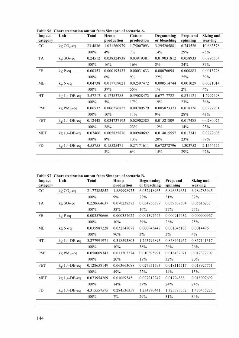
144
Table 96: Characterization output from Simapro of scenario A. Impact category
Unit Total Hemp production
Cotton production
Degumming or bleaching
Prep. and spinning
Sizing and weaving
CC kg CO2-eq 23.4836 1.031260979 1.75007093 3.295205881 6.743526 10.663578 100% 4% 7% 14% 29% 45% TA kg SO2-eq 0.24512 0.038324938 0.03919381 0.019031812 0.058933 0.0896354 100% 16% 16% 8% 24% 37% FE kg P-eq 0.00353 0.000195133 0.00031633 0.00076094 0.000883 0.0013728 100% 6% 9% 22% 25% 39% ME kg N-eq 0.04738 0.017759021 0.02597472 0.000514744 0.001029 0.0021014 100% 37% 55% 1% 2% 4% HT kg 1,4-DB-eq 3.57217 0.17383785 0.59028472 0.67717722 0.831121 1.2997498 100% 5% 17% 19% 23% 36% PMF kg PM10-eq 0.06532 0.006276822 0.00709579 0.005823373 0.018326 0.0277931 100% 10% 11% 9% 28% 43% FET kg 1,4-DB-eq 0.12448 0.034737193 0.02902585 0.01521809 0.017488 0.0280075 100% 28% 23% 12% 14% 23% MET kg 1,4-DB-eq 0.07466 0.005835876 0.00940692 0.014815557 0.017341 0.0272608 100% 8% 13% 20% 23% 37% FD kg 1,4-DB-eq 4.55755 0.15525471 0.27171611 0.672372796 1.303752 2.1544555
3% 6% 15% 29% 47%
Table 97: Characterization output from Simapro of scenario B. Impact category
Unit Total Hemp production
Degumming or bleaching
Prep. and spinning
Sizing and weaving
CC kg CO2-eq 21.77385852 1.889998975 6.052418965 6.846654631 6.984785945 100% 9% 28% 31% 32% TA kg SO2-eq 0.220664637 0.070238373 0.034956389 0.059307504 0.05616237 100% 32% 16% 27% 25% FE kg P-eq 0.003570666 0.000357622 0.001397645 0.000914432 0.000900967 100% 10% 39% 26% 25% ME kg N-eq 0.035987228 0.032547078 0.000945447 0.001045103 0.0014496 100% 90% 3% 3% 4% HT kg 1,4-DB-eq 3.277991971 0.318593803 1.243794893 0.858461957 0.857141317 100% 10% 38% 26% 26% PMF kg PM10-eq 0.058009343 0.011503574 0.010695991 0.018437071 0.017372707 100% 20% 18% 32% 30% FET kg 1,4-DB-eq 0.128658149 0.063663088 0.027951593 0.018115717 0.018927751 100% 49% 22% 14% 15% MET kg 1,4-DB-eq 0.073954269 0.01069545 0.027212247 0.01794888 0.018097692 100% 14% 37% 24% 24% FD kg 1,4-DB-eq 4.315557575 0.284536357 1.234970441 1.325595552 1.470455225
100% 7% 29% 31% 34%

145
Table 98: Characterization output from Simapro of scenario C. Impact category
Unit Total Hemp production
Degumming or bleaching
Prep. and spinning
Sizing and weaving
CC kg CO2-eq 31.8292476 2.18755266 4.78542733 8.708259029 16.14800858 100% 7% 15% 27% 51% TA kg SO2-eq 0.324304131 0.081296415 0.032575013 0.072383893 0.13804881 100% 25% 10% 22% 43% FE kg P-eq 0.004607833 0.000413925 0.000946904 0.001167378 0.002079627 100% 9% 21% 25% 45% ME kg N-eq 0.042521489 0.037671157 0.000649803 0.001278977 0.002921552 100% 89% 2% 3% 7% HT kg 1,4-DB-eq 4.290639817 0.368751905 0.842215784 1.113564863 1.966107266 100% 9% 20% 26% 46% PMF kg PM10-eq 0.088678095 0.01331465 0.010013861 0.022495718 0.042853866 100% 15% 11% 25% 48% FET kg 1,4-DB-eq 0.15848019 0.073685944 0.018283312 0.024540547 0.041970386 100% 46% 12% 15% 26% MET kg 1,4-DB-eq 0.095180124 0.012379297 0.017905679 0.023761093 0.041134055 100% 13% 19% 25% 43% FD kg 1,4-DB-eq 6.259723017 0.329332594 0.948248665 1.771818582 3.210323177
100% 5% 15% 28% 51%
Figure 21: Agricultural land occupation of four fabric scenarios. This figure presents a graphical representation of the agricultural land occupation for 1 kg fabric in the four different fabric scenarios.

146
Appendix 10 Biogenic carbon sequestration
Appendix 10.1 Calculation of biogenic carbon content in cotton and hemp
Table 99: Back-of-the-envelope calculations of CO2-sequestration in hemp and cotton fibres. CO2(i) = CC * TY(i) * W(CO2) * EA(i) / FY(i) CO2(i) = Biogenic CO2 sequestered per kg of fibre (i = hemp or cotton)
For i = Hemp Cotton = 3.76 kg per kg fibre 3.21 kg per kg fibre CC = Average carbon content of dry biomass = 47.5% TY(i) = Total harvested dry matter yield
For i = Hemp Cotton = 9000 3843 W(CO2) = Factor for multiplying CO2-C weight to CO2 weight = 44/12 EA = Economic allocation to the fibre
For i = Hemp Cotton = 53% 72% FY(i) = Fibre yield
For i = Hemp Cotton = 2200 kg per hectare 1486 kg per hectare


