Bivariate data analysis

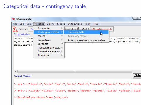
Categorical data - creating data set

Upload the following data set to R Commander

sex female male male male male female female male female femaleeye black black blue green green green black green blue blue

I Method 1: Type the table in the Notepad, save it and importto Rcmdr

I Method 2: Introduce directly in the Script Window

eye = c("black","black","blue","green","green",

"green","black","green","blue","blue")

sex = c("female","male","male","male","male",

"female", "female","male","female","female")

DataSexEye = data.frame(sex ,eye)

Categorical data - contingency table

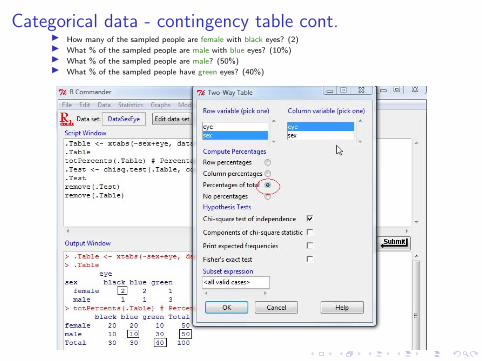
Categorical data - contingency table cont.I How many of the sampled people are female with black eyes? (2)I What % of the sampled people are male with blue eyes? (10%)I What % of the sampled people are male? (50%)I What % of the sampled people have green eyes? (40%)

Categorical data - barchart

I Load the library lattice, then create barchart grouping thedata by sex

library(lattice)

barchart(DataSexEye , groups=DataSexEye$sex)

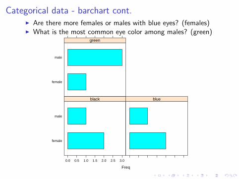
Categorical data - barchart cont.I Are there more females or males with blue eyes? (females)I What is the most common eye color among males? (green)

Freq

female

male

0.0 0.5 1.0 1.5 2.0 2.5 3.0

black blue

female

male

green

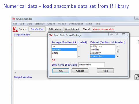
Numerical data - load anscombe data set from R library

Numerical data - scatterplot of y1 versus x1

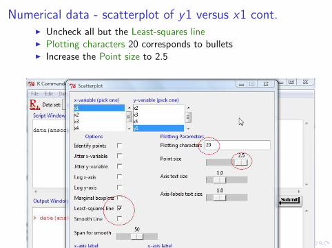
Numerical data - scatterplot of y1 versus x1 cont.I Uncheck all but the Least-squares lineI Plotting characters 20 corresponds to bulletsI Increase the Point size to 2.5

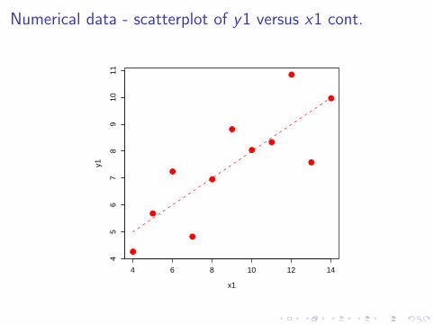
Numerical data - scatterplot of y1 versus x1 cont.

4 6 8 10 12 14

45

67

89

1011

x1

y1

●

●

●

●

●

●

●

●

●

●

●

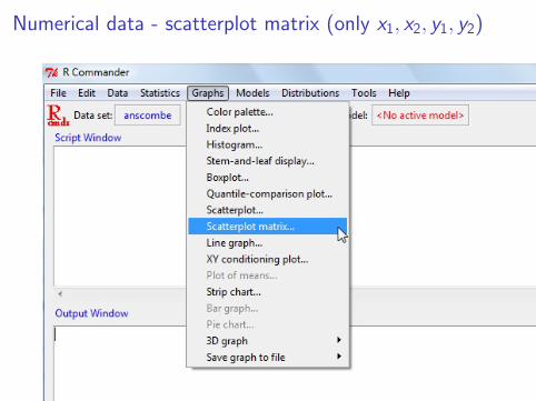
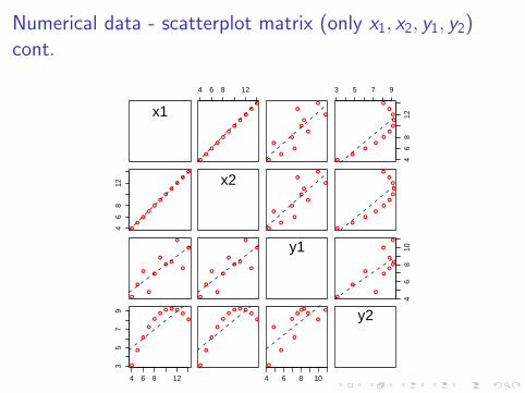
Numerical data - scatterplot matrix (only x1, x2, y1, y2)

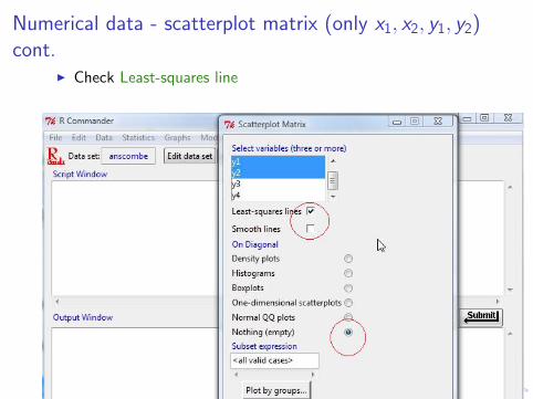
Numerical data - scatterplot matrix (only x1, x2, y1, y2)cont.

I Check Least-squares line

Numerical data - scatterplot matrix (only x1, x2, y1, y2)cont.

x1

4 6 8 12

●

●

●

●

●

●

●

●

●

●

●

●

●

●

●

●

●

●

●

●

●

●

3 5 7 9

46

812

●

●

●

●

●

●

●

●

●

●

●

46

812

●

●

●

●

●

●

●

●

●

●

●

x2●

●

●

●

●

●

●

●

●

●

●

●

●

●

●

●

●

●

●

●

●

●

●

●

●

●●

●

●

●

●

●

●

●

●

●

●●

●

●

●

●

●

●

y1

46

810

●

●

●

●●

●

●

●

●

●

●

4 6 8 12

35

79 ●

●

●●●

●

●

●

●

●

●

●

●

●●●

●

●

●

●

●

●

4 6 8 10

●

●

● ●●

●

●

●

●

●

●

y2

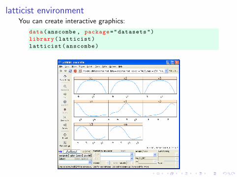
latticist environmentYou can create interactive graphics:

data(anscombe , package="datasets")

library(latticist)

latticist(anscombe)

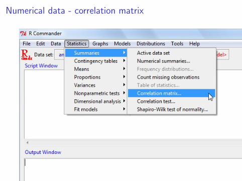
Numerical data - correlation matrix

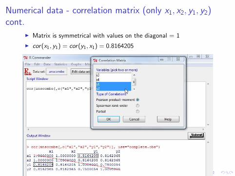
Numerical data - correlation matrix (only x1, x2, y1, y2)cont.

I Matrix is symmetrical with values on the diagonal = 1

I cor(x1, y1) = cor(y1, x1) = 0.8164205

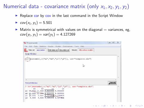
Numerical data - covariance matrix (only x1, x2, y1, y2)

I Replace cor by cov in the last command in the Script Window

I cov(x1, y1) = 5.501

I Matrix is symmetrical with values on the diagonal = variances, eg,cov(y1, y1) = var(y1) = 4.127269

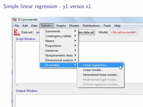
Simple linear regression - y1 versus x1

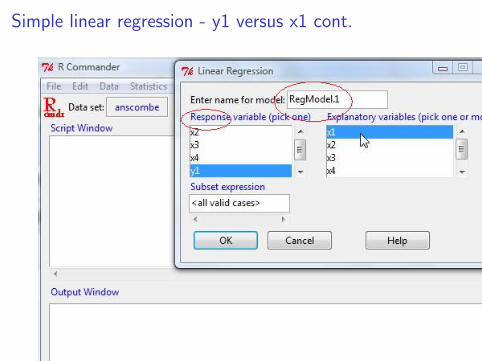
Simple linear regression - y1 versus x1 cont.

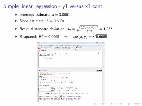
Simple linear regression - y1 versus x1 cont.

I Intercept estimate: a = 3.0001

I Slope estimate: b = 0.5001

I Residual standard deviation: sR =√∑n

i=1(yi−yi )2

n−2 = 1.237

I R-squared: R2 = 0.6665 ⇒ cor(x , y) =√

0.6665

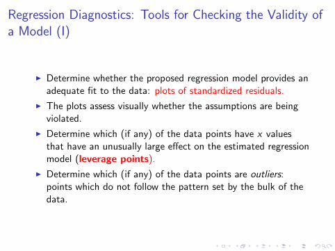
Regression Diagnostics: Tools for Checking the Validity ofa Model (I)

I Determine whether the proposed regression model provides anadequate fit to the data: plots of standardized residuals.

I The plots assess visually whether the assumptions are beingviolated.

I Determine which (if any) of the data points have x valuesthat have an unusually large effect on the estimated regressionmodel (leverage points).

I Determine which (if any) of the data points are outliers:points which do not follow the pattern set by the bulk of thedata.

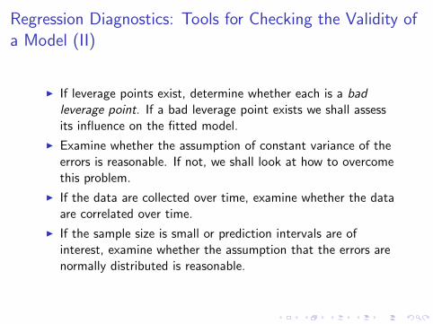
Regression Diagnostics: Tools for Checking the Validity ofa Model (II)

I If leverage points exist, determine whether each is a badleverage point. If a bad leverage point exists we shall assessits influence on the fitted model.

I Examine whether the assumption of constant variance of theerrors is reasonable. If not, we shall look at how to overcomethis problem.

I If the data are collected over time, examine whether the dataare correlated over time.

I If the sample size is small or prediction intervals are ofinterest, examine whether the assumption that the errors arenormally distributed is reasonable.

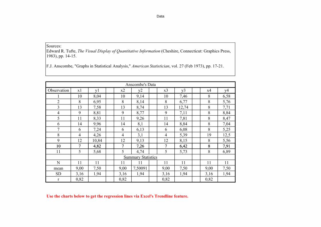
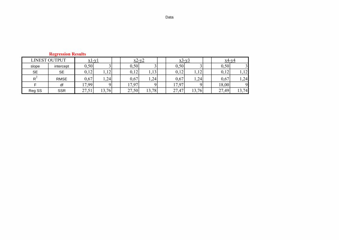
Data

Anscombe's Data

Observation x1 y1 x2 y2 x3 y3 x4 y4

1 10 8,04 10 9,14 10 7,46 8 6,58

2 8 6,95 8 8,14 8 6,77 8 5,76

3 13 7,58 13 8,74 13 12,74 8 7,71

4 9 8,81 9 8,77 9 7,11 8 8,84

5 11 8,33 11 9,26 11 7,81 8 8,47

6 14 9,96 14 8,1 14 8,84 8 7,04

7 6 7,24 6 6,13 6 6,08 8 5,25

8 4 4,26 4 3,1 4 5,39 19 12,5

9 12 10,84 12 9,13 12 8,15 8 5,56

10 7 4,82 7 7,26 7 6,42 8 7,91

Sources:

Edward R. Tufte, The Visual Display of Quantitative Information (Cheshire, Connecticut: Graphics Press,

1983), pp. 14-15.

F.J. Anscombe, "Graphs in Statistical Analysis," American Statistician, vol. 27 (Feb 1973), pp. 17-21.

10 7 4,82 7 7,26 7 6,42 8 7,91

11 5 5,68 5 4,74 5 5,73 8 6,89

Summary Statistics

N 11 11 11 11 11 11 11 11

mean 9,00 7,50 9,00 7,50091 9,00 7,50 9,00 7,50

SD 3,16 1,94 3,16 1,94 3,16 1,94 3,16 1,94

r 0,82 0,82 0,82 0,82

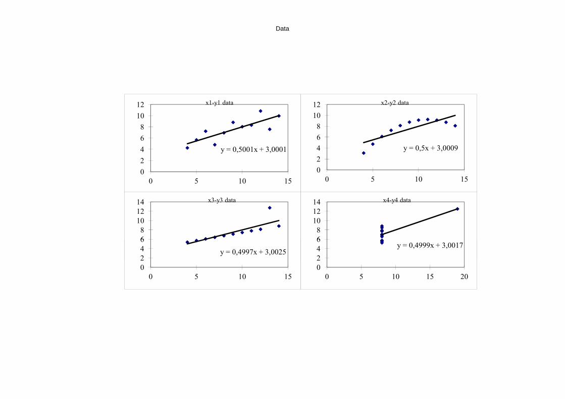
Use the charts below to get the regression lines via Excel's Trendline feature.

Data

0

2

4

6

8

10

12

14

0 5 10 15 20

x1-y1

0

2

4

6

8

10

12

14

0 5 10 15 20

x2-y2

4

6

8

10

12

14x3-y3

468

101214

x4-y4

0

2

4

6

8

0 5 10 15 20

02468

0 5 10 15 20

Data

Regression Results

slope intercept 0,50 3 0,50 3 0,50 3 0,50 3

SE SE 0,12 1,12 0,12 1,13 0,12 1,12 0,12 1,12

R2

RMSE 0,67 1,24 0,67 1,24 0,67 1,24 0,67 1,24

F df 17,99 9 17,97 9 17,97 9 18,00 9

Reg SS SSR 27,51 13,76 27,50 13,78 27,47 13,76 27,49 13,74

x4-y4LINEST OUTPUT x1-y1 x2-y2 x3-y3

Data

y = 0,5001x + 3,0001

0

2

4

6

8

10

12

0 5 10 15

x1-y1 data

y = 0,5x + 3,0009

0

2

4

6

8

10

12

0 5 10 15

x2-y2 data

y = 0,4997x + 3,00252

4

6

8

10

12

14 x3-y3 data

y = 0,4999x + 3,0017

2

4

6

8

10

12

14 x4-y4 data

y = 0,4997x + 3,0025

0

2

4

6

0 5 10 15

y = 0,4999x + 3,0017

0

2

4

6

0 5 10 15 20

Simple linear regression - residual plot (method 1)

Simple linear regression - residual plot (method 1) cont.I Residuals versus fitted (top left plot)

5 6 7 8 9 10

−2

−1

01

2

Fitted values

Res

idua

ls

●●

●

●

● ●

●

●

●

●

●

Residuals vs Fitted

3

9

10

●●

●

●

● ●

●

●

●

●

●

−1.5 −0.5 0.5 1.5

−1

01

2

Theoretical Quantiles

Sta

ndar

dize

d re

sidu

als

Normal Q−Q

3

9

10

5 6 7 8 9 10

0.0

0.4

0.8

1.2

Fitted values

Sta

ndar

dize

d re

sidu

als

●●

●

●

●

●

●

●

●●

●

Scale−Location39

10

0.00 0.10 0.20 0.30

−2

−1

01

2

Leverage

Sta

ndar

dize

d re

sidu

als

●●

●

●

● ●

●

●

●

●

●

Cook's distance1

0.5

0.5

1Residuals vs Leverage

3

9

10

lm(y1 ~ x1)

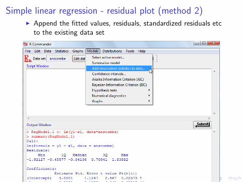
Simple linear regression - residual plot (method 2)I Append the fitted values, residuals, standardized residuals etc

to the existing data set

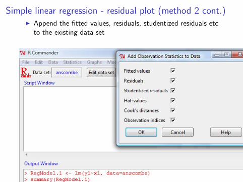
Simple linear regression - residual plot (method 2 cont.)I Append the fitted values, residuals, studentized residuals etc

to the existing data set

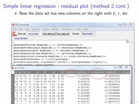
Simple linear regression - residual plot (method 2 cont.)I Now the data set has new columns on the right with y , r , etc

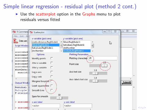
Simple linear regression - residual plot (method 2 cont.)I Use the scatterplot option in the Graphs menu to plot

residuals versus fitted

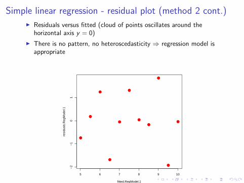
Simple linear regression - residual plot (method 2 cont.)

I Residuals versus fitted (cloud of points oscillates around thehorizontal axis y = 0)

I There is no pattern, no heteroscedasticity ⇒ regression model isappropriate

5 6 7 8 9 10

−2

−1

01

fitted.RegModel.1

resi

dual

s.R

egM

odel

.1

●●

●

●

●●

●

●

●

●

●

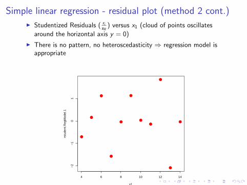
Simple linear regression - residual plot (method 2 cont.)

I Studentized Residuals ( risR

) versus x1 (cloud of points oscillates

around the horizontal axis y = 0)

I There is no pattern, no heteroscedasticity ⇒ regression model isappropriate

4 6 8 10 12 14

−2

−1

01

x1

rstu

dent

.Reg

Mod

el.1

●●

●

●

●●

●

●

●

●

●