Binary Logistic Regression

Background and Examples, Binary Logistic Regression in R, and Communicating Results

Prepared by Allison Horst for ESM 244

Bren School of Environmental Science & Management, UCSB Introduction, Conceptual Background and Examples Binary logistic regression is used to understand relationships between one or more independent variables (measured or categorical) and a dichotomous dependent variable (i.e., a variable with only two possible outcomes: yes/no, pass/fail, live/die, etc.). Logistic regression is particularly useful in determining the probability of a categorical outcome occurring based on the value or category of input variable(s). Examples that may benefit from analysis by logistic regression:

Example 1. You measure patient blood pressure and heart rate, and want to understand how they influence the probability of a patient having a heart attack within the next 5 years.

Independent measurement variables: blood pressure and heart rate. Dichotomous dependent variable: heart attack/no heart attack within 5 years.

Example 2. How do gender and age influence a person’s likelihood to vote in an election?

Independent categorical variables: gender and age. Dichotomous dependent variable: votes/does not vote.

Logistic regression explores the odds of an event occurring. The odds ratio is the probability of an event occurring divided by the probability of the event not occurring:

!""# =  !

1 − !

The log odds of an event (also called the logit) are given by:

ln!

1 − ! = !"#$% ! = !! + !!!! +⋯+ !!!!

Where the coefficients (β) are determined from the logistic regression model (see approach in R below), and the variables (x1, x2, …xn) are the values of the independent variables. If the independent variables are measured, the values are input directly. If the independent variables are categorical, the use of dummy variables is required. Dummy variables (typically) assign a value of 0 or 1 to categorical input variables and dichotomous dependent variables. For example, using Example 2 above, we might code the dichotomous dependent variable as [Does Not Vote = 0, Votes = 1], and the categorical input variable (gender) as [Female = 0, Male = 1]. Thus, categorical information is coded as quantitative information using proxies (also called Boolean operators).

Since we have an expression for the log odds (above), we can convert (using the exponential) that equation into an expression for the odds as follows:

!

1 − != !(!!!!!!!!⋯ )

And, if we want to express the probability of the outcome, we can rewrite the equation as:

! =!(!!!!!!!!⋯ )

1 + !(!!!!!!!!⋯ )

So if we know the coefficients (β0, β1, … βn), and we know the values of the input variables x1…xn (either as measured values or coded dummy variables), then to find the probability of an outcome we can use the equation above. Before moving on to how to determine the coefficients in R, let’s take a look at a simple (fictional) example to see how the equations above are useful in interpreting logistic regression results.

Example: One categorical input variable, one dichotomous dependent variable.

A researcher is investigating the influence of gender (Female = 0, Male = 1) on the likelihood of a child having an attention disorder (dichotomous: yes/no for disorder/no disorder). Logistic regression yields the following:

!"#$%  ! =  −1.45 + 1.61 ∗ !"#$"%

What are the odds of a female child having an attention disorder?

The log odds are found by:

!"#$%  ! =  −1.45 + 1.61 ∗ 0 =  −1.45 So the odds of a girl having an attention disorder is calculated by:

!1 − ! = !(!!!!!!!!⋯ ) = !!!.!" = 0.234

What are the odds of a male child having an attention disorder? The log odds are found by:

!"#$%  ! =  −1.45 + 1.61 ∗ 1 =  0.16

So the odds of a boy having an attention disorder is calculated by:

!1 − ! = !(!!!!!!!!⋯ ) = !!.!" = 1.17

How do the odds for boys and girls compare? You find the comparison of odds two ways: by dividing the boys odds by the girls odds (1.17/0.23 = 5.00), or simply by taking the exponential of the coefficient in front of the

gender term (here, β1), to similarly find an odds ratio (male:female) by e1.61 = 5.00. Either way, you see that the relative odds of a boy having an attention disorder compared to a girl is ~5. What if you have a measured predictor variable? Below, consider the example (in which you are trying to predict the odds of a rat contracting a tumor when exposed to varying dosages of a chemical. Example (based on example described in lecture by Dr. Bruce Kendall in ESM 244): One continuous (measured) input variable, one dichotomous dependent variable.

You are investigating the influence of a chemical dosage (in ppm) on tumor formation in rats, where the dependent variable is dichotomous (no tumor/tumor). Performing logistic regression yields the following expression:

!"#$%  ! = −4.34+ 0.013 ∗ !"#$  

What types of information can we get from this expression? A lot! In fact, you can explore the complete logistic model to determine likelihood of tumor formation at any concentration! But let’s start by considering some simple ways to think about it:

What are the odds of a rat contracting a tumor at a dosage of 250 ppm?

!"#$%  ! =  −4.34 + 0.013 ∗ 250 =  −1.09

!

1 − != !!!.!" = 0.34

And the probability of a rat contracting a tumor at a dosage of 250 ppm?

Rearrange the above equation and solve for P to find: P250 = 0.25. Or, based on this model there is a 25% chance that a rate exposed to 250 ppm of the chemical will develop a tumor.

Another interesting question might be to ask: at what dosage is there a 50% likelihood that a rat will develop a tumor? We can again use the logit expression, substituting 0.5 in for ‘P’:

ln!

1 − ! = !! + !!!! +⋯+ !!!! = −4.34 + 0.013 ∗ !"#$

ln0.5

1 − 0.5 = −4.34 + 0.013 ∗ !"#$

0 = −4.34 + 0.013 ∗ !"#$

Dose = 334  ppm

So the dose at which the likelihood of a rat developing a tumor is 50% is 334 ppm (these are slightly different that reported in the lecture, due to rounding).

Example: Multiple (>1) predictor variables and one dichotomous dependent variable.

Often, you will have multiple predictor variables (categorical, measured, or a mix!) that influence the outcome of a dichotomous dependent variable. In those cases, it can also be useful to perform logistic regression.

Let’s consider another example. A researcher is studying the influence of systolic blood pressure (SBP; mm Hg) and heart rate (HR; bpm) on likelihood of male over the age of 85 having a heart attack (no heart attack = 0, heart attack = 1). Logistic regression yields the following:

!"#$%  ! =  −5.09+ 0.015 ∗ !"# + 0.043 ∗ !"

As above, we can easily answer questions about the odds of a heart attack for varying values of BP and HR.

What are the odds of a heart attack occurring for a patient with a SBP of 138 and HR of 76?

!

1 − ! = !(!!!!!!!!⋯ ) = !(!!.!"!!.!"#∗!"#!!.!"#∗!") = 1.28

Since the odds are 1.28, the probability of a heart attack is solved by rearranging the odds equation to yield P = 0.56.

It can also be interesting to think about the influence of the individual predictor variables on the outcome likelihood. What can we learn from the coefficients for each independent variable?

Well, we know that the coefficient for SBP is 0.015, which means that the odds ratio for that component is e0.015 = 1.015. We can interpret the value as follows: for every one unit increase in SBP, males over the age of 85 are 1.015 times more likely to suffer a heart attack. Similarly, if we consider the influence of HR, the odds ratio is e0.043 = 1.043, which we can interpret as follows: for every one unit increase in HR, the likelihood of having a heart attack is increased 1.043 times. Or, an alternate way to say this is: for every one unit increase in heart rate, the likelihood of a man over 85 years old having a heart attack is increased by 4.3%.

Binary Logistic Regression in R

**You can download an Excel file with the sheep data used in the example below to follow along – in the example below, the data frame is loaded from a .csv file called ‘Sheep.’ So now you (hopefully!) have an idea of when, how and why logistic regression can be useful. There are two major things left to learn: how to do it (how do I find those coefficients?) and how to communicate the results graphically and in text.

Luckily, once you understanding the basics of logistic regression, finding the coefficients in R is pretty straightforward using the glm() function (where ‘glm’ stands for generalized linear model). Here, an example will be used to demonstrate binary logistic regression in R.

Let’s consider a (fictional) dataset for which male bighorn sheep weight (in lbs) is used as a predictor variable for the success of male bighorn sheep in finding a mate (no mate = 0, mate = 1). The first 5 lines of the dataset are shown below (67 sheep total):

. . . .

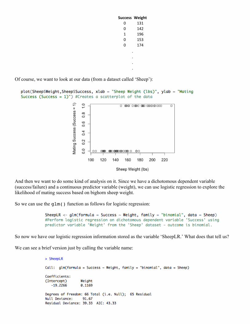
Of course, we want to look at our data (from a dataset called ‘Sheep’):

And then we want to do some kind of analysis on it. Since we have a dichotomous dependent variable (success/failure) and a continuous predictor variable (weight), we can use logistic regression to explore the likelihood of mating success based on bighorn sheep weight.

So we can use the glm() function as follows for logistic regression:

So now we have our logistic regression information stored as the variable ‘SheepLR.’ What does that tell us? We can see a brief version just by calling the variable name:

!"##$%% &$'()*! "#"! "$%" "&'! "(#! ")$

Which provides the coefficients for the logit (β0 = -19.22, β1 = 0.1169). So, just using the glm() function we are able to find the expression:

!"#$%  ! = ln!

1− ! = −19.22+ 0.1169 ∗!"#$ℎ!

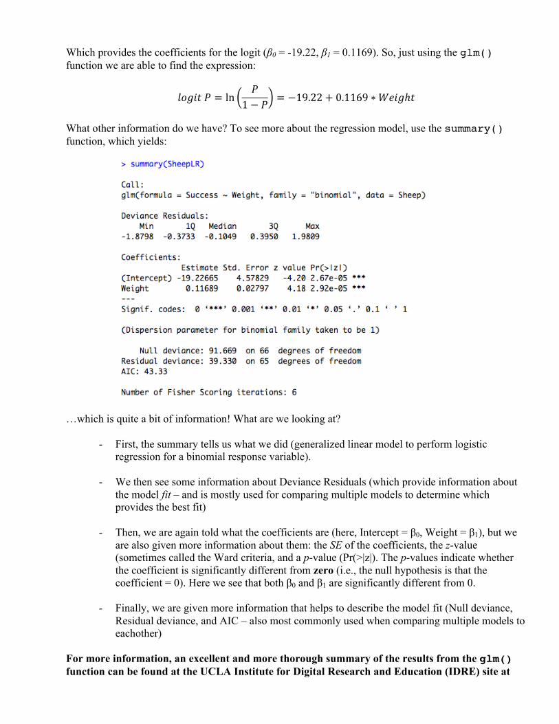
What other information do we have? To see more about the regression model, use the summary() function, which yields:

…which is quite a bit of information! What are we looking at?

- First, the summary tells us what we did (generalized linear model to perform logistic regression for a binomial response variable).

- We then see some information about Deviance Residuals (which provide information about the model fit – and is mostly used for comparing multiple models to determine which provides the best fit)

- Then, we are again told what the coefficients are (here, Intercept = β0, Weight = β1), but we

are also given more information about them: the SE of the coefficients, the z-value (sometimes called the Ward criteria, and a p-value (Pr(>|z|). The p-values indicate whether the coefficient is significantly different from zero (i.e., the null hypothesis is that the coefficient = 0). Here we see that both β0 and β1 are significantly different from 0.

- Finally, we are given more information that helps to describe the model fit (Null deviance,

Residual deviance, and AIC – also most commonly used when comparing multiple models to eachother)

For more information, an excellent and more thorough summary of the results from the glm() function can be found at the UCLA Institute for Digital Research and Education (IDRE) site at

http://www.ats.ucla.edu/stat/r/dae/logit.htm. There are also really great graphics examples at that site!

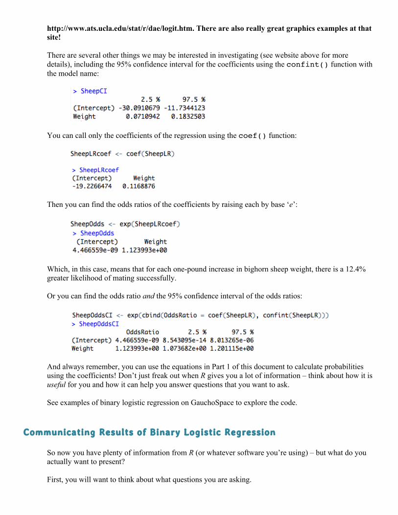
There are several other things we may be interested in investigating (see website above for more details), including the 95% confidence interval for the coefficients using the confint() function with the model name:

You can call only the coefficients of the regression using the coef() function:

Then you can find the odds ratios of the coefficients by raising each by base ‘e’:

Which, in this case, means that for each one-pound increase in bighorn sheep weight, there is a 12.4% greater likelihood of mating successfully. Or you can find the odds ratio and the 95% confidence interval of the odds ratios:

And always remember, you can use the equations in Part 1 of this document to calculate probabilities using the coefficients! Don’t just freak out when R gives you a lot of information – think about how it is useful for you and how it can help you answer questions that you want to ask. See examples of binary logistic regression on GauchoSpace to explore the code.

Communicating Results of Binary Logistic Regression

So now you have plenty of information from R (or whatever software you’re using) – but what do you actually want to present? First, you will want to think about what questions you are asking.

For example, to use the bighorn example above, you might ask if it is helpful to:

- Calculate the sheep weight at which there is a 50% chance of the sheep mating successfully? - Determine he probability that a sheep weighing 140 lbs will mate successfully? - Calculate the increase in likelihood of a male bighorn mating successfully with each 1 lb

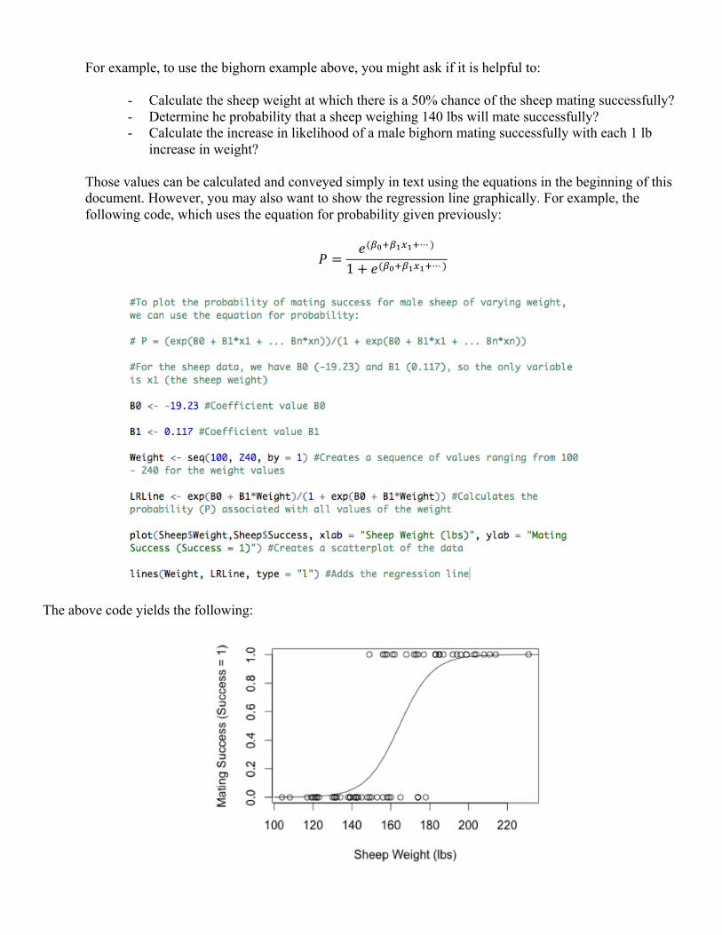
increase in weight? Those values can be calculated and conveyed simply in text using the equations in the beginning of this document. However, you may also want to show the regression line graphically. For example, the following code, which uses the equation for probability given previously:

! =!(!!!!!!!!⋯ )

1+ !(!!!!!!!!⋯ )

The above code yields the following:

In addition to a graphical representation of the logistic regression, you may also want to write out the equation explicitly. For the sheep example, you would probably want to include the equation as (make sure to let the audience know the units of the predictor variables – here, ‘Weight’ is bighorn sheep weight in pounds):

ln!

1− ! = −19.23+ 0.117 ∗!"#$ℎ!

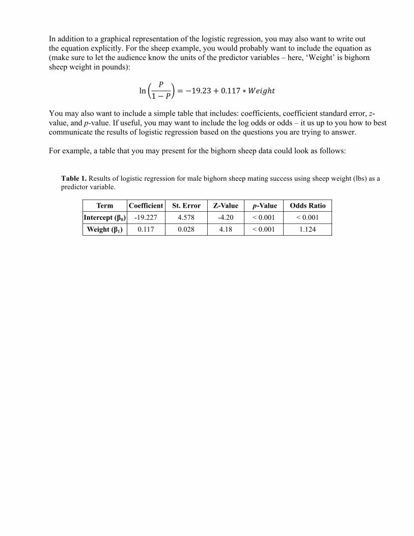
You may also want to include a simple table that includes: coefficients, coefficient standard error, z-value, and p-value. If useful, you may want to include the log odds or odds – it us up to you how to best communicate the results of logistic regression based on the questions you are trying to answer.

For example, a table that you may present for the bighorn sheep data could look as follows:

Table 1. Results of logistic regression for male bighorn sheep mating success using sheep weight (lbs) as a predictor variable.

Term Coefficient St. Error Z-Value p-Value Odds RatioIntercept (!0) -19.227 4.578 -4.20 < 0.001 < 0.001Weight (!1) 0.117 0.028 4.18 < 0.001 1.124