Download - An empirical investigation of economic growth and debt

University of PiraeusDepartment of Economics

An empirical investigation of economic growth and debt

Dimitrios KiritsisDonatela SalaiAntzela Ouroutsi

Piraeus, June 2015

05/02/23

Outline• Motivation• Graph• Model• Data• Results• Estimated Model• Robustness • Conclusions / References

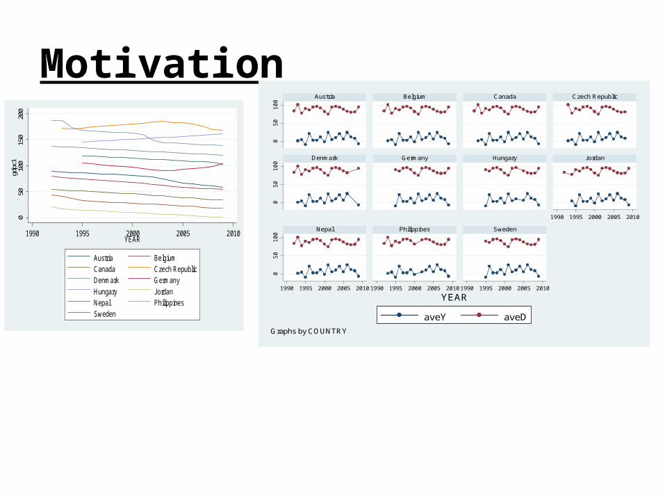
Motivation

050

100

050

100

050

100

1990 1995 2000 2005 2010

1990 1995 2000 2005 2010 1990 1995 2000 2005 2010 1990 1995 2000 2005 2010

Austria Belgium Canada Czech Republic

Denmark Germany Hungary Jordan

Nepal Philippines Sweden

aveY aveD

YEAR

Graphs by COUNTRY

050

100

150

200

gdpc

1

1990 1995 2000 2005 2010YEAR

Austria BelgiumCanada Czech RepublicDenmark GermanyHungary JordanNepal PhilippinesSweden

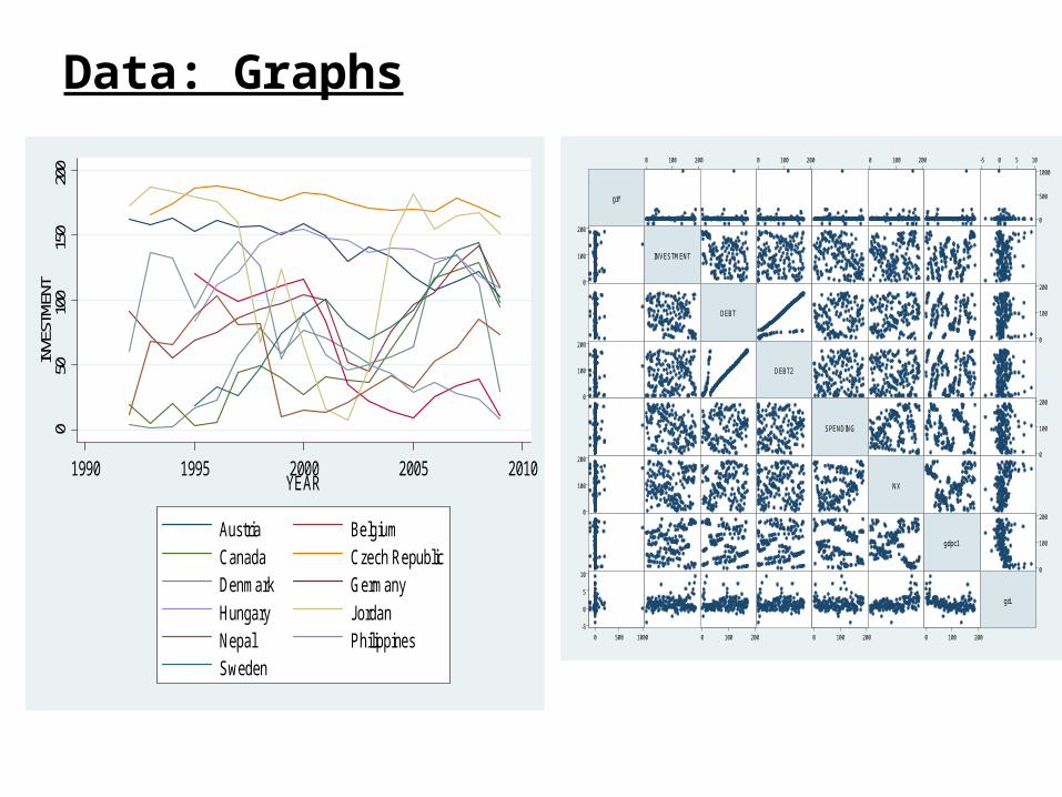
Data: Graphs0

5010

015

020

0IN

VESTM

ENT

1990 1995 2000 2005 2010YEAR


grY

INVESTMENT

DEBT

DEBT2

SPENDING

NX

gdpc1

grL

0

500

1000

0 500 1000

0

100

200

0 100 200

0

100

200

0 100 200

0

100

200

0 100 200

0

100

200

0 100 200

0

100

200

0 100 200

0

100

200

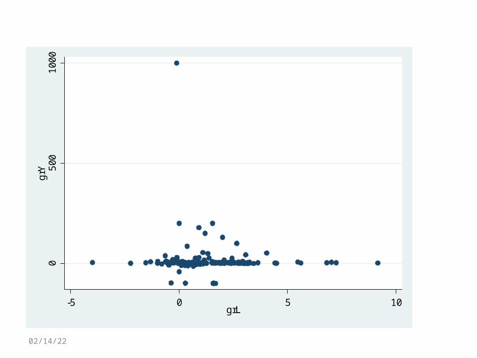
0 100 200-5

0

5

10

-5 0 5 10

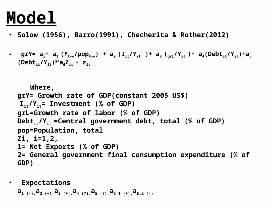
Model

• Solow (1956), Barro(1991), Checherita & Rother(2012)

• grY= ai+ a1 (Yt=o/popt=o) + a2 (Iit/Yit )+ a3 (grL/Yit )+ a4(Debtit/Yit)+a5 (Debtit/Yit)2+a6Zit + εit

Where, grY= Growth rate of GDP(constant 2005 US$) Iit/Yit= Investment (% of GDP)grL=Growth rate of labor (% of GDP)Debtit/Yit =Central government debt, total (% of GDP)pop=Population, totalZi, i=1,2,1= Net Exports (% of GDP) 2= General government final consumption expenditure (% of GDP)

• Expectations

a1 (-),a2 (+),a3 (+),a4 (?),a5 (?),a6.1 (+),a6.2 (-)

Data• Countries : Austria, Canada, Czech Republic, Denmark,

Hungary, Jordan, Nepal, Philippines, Sweden

• Time span : 1992/1995-2009

• Source : World Bank Indicator (WDI)

Results

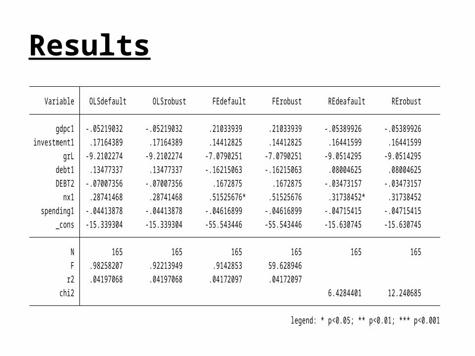
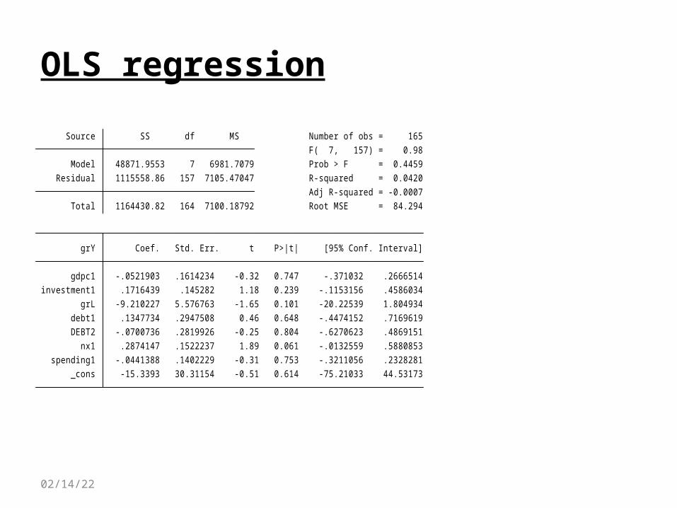
legend: * p<0.05; ** p<0.01; *** p<0.001 chi2 6.4284401 12.240685 r2 .04197068 .04197068 .04172097 .04172097 F .98258207 .92213949 .9142853 59.628946 N 165 165 165 165 165 165 _cons -15.339304 -15.339304 -55.543446 -55.543446 -15.630745 -15.630745 spending1 -.04413878 -.04413878 -.04616899 -.04616899 -.04715415 -.04715415 nx1 .28741468 .28741468 .51525676* .51525676 .31738452* .31738452 DEBT2 -.07007356 -.07007356 .1672875 .1672875 -.03473157 -.03473157 debt1 .13477337 .13477337 -.16215063 -.16215063 .08004625 .08004625 grL -9.2102274 -9.2102274 -7.0790251 -7.0790251 -9.0514295 -9.0514295 investment1 .17164389 .17164389 .14412825 .14412825 .16441599 .16441599 gdpc1 -.05219032 -.05219032 .21033939 .21033939 -.05389926 -.05389926 Variable OLSdefault OLSrobust FEdefault FErobust REdeafault RErobust

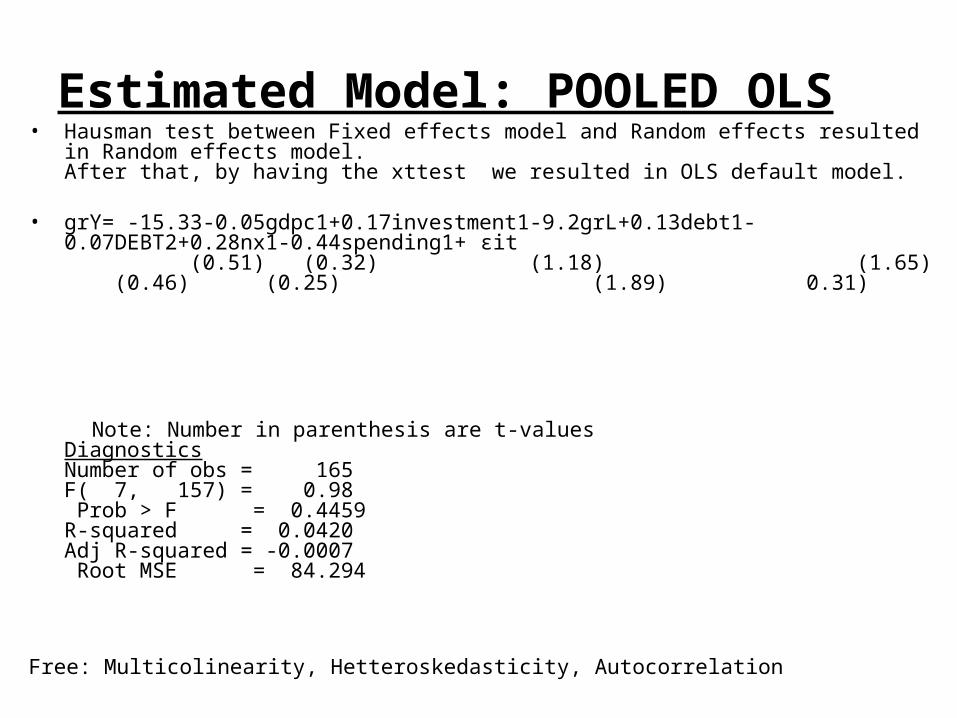
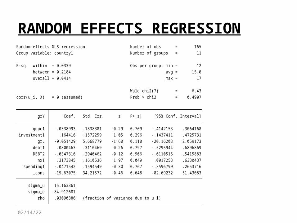
Estimated Model: POOLED OLS• Hausman test between Fixed effects model and Random effects resulted in Random effects model.

After that, by having the xttest we resulted in OLS default model.

• grY= -15.33-0.05gdpc1+0.17investment1-9.2grL+0.13debt1-0.07DEBT2+0.28nx1-0.44spending1+ εit (0.51) (0.32) (1.18) (1.65) (0.46) (0.25) (1.89) 0.31)

Note: Number in parenthesis are t-valuesDiagnosticsNumber of obs = 165F( 7, 157) = 0.98 Prob > F = 0.4459 R-squared = 0.0420Adj R-squared = -0.0007 Root MSE = 84.294

Free: Multicolinearity, Hetteroskedasticity, Autocorrelation

05/02/23

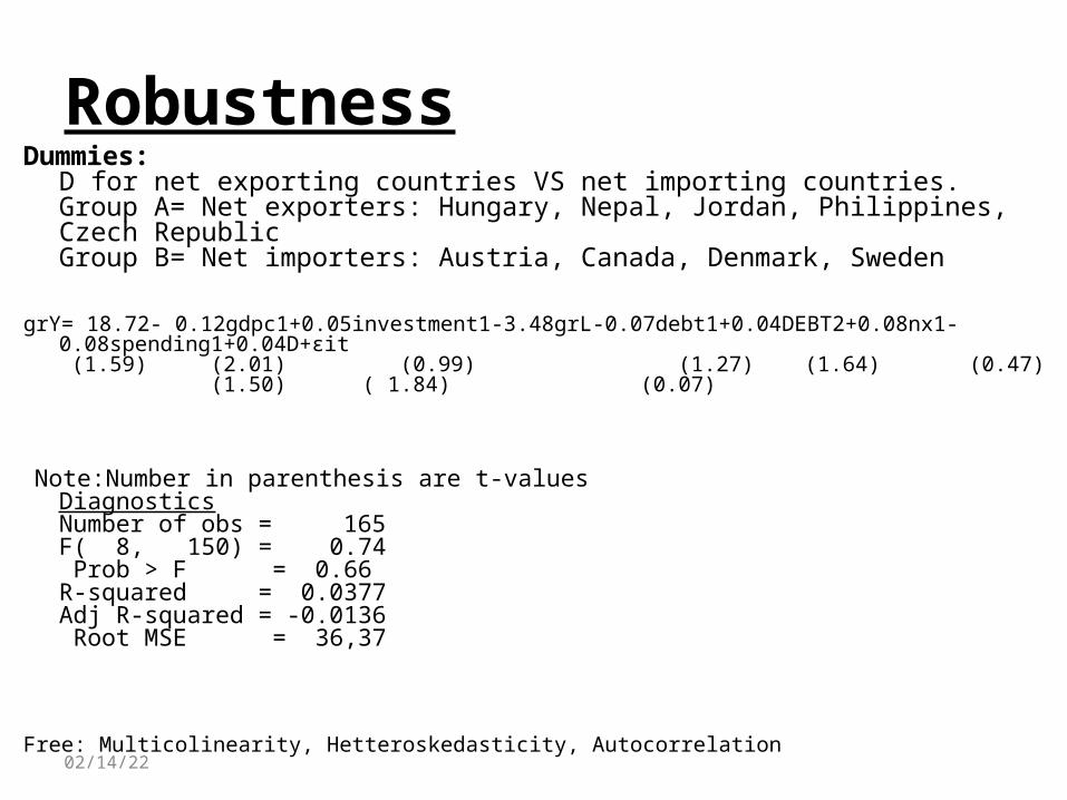
RobustnessDummies:

D for net exporting countries VS net importing countries.Group A= Net exporters: Hungary, Nepal, Jordan, Philippines, Czech RepublicGroup B= Net importers: Austria, Canada, Denmark, Sweden

grY= 18.72- 0.12gdpc1+0.05investment1-3.48grL-0.07debt1+0.04DEBT2+0.08nx1-0.08spending1+0.04D+εit (1.59) (2.01) (0.99) (1.27) (1.64) (0.47) (1.50) ( 1.84) (0.07)

Note:Number in parenthesis are t-values

DiagnosticsNumber of obs = 165F( 8, 150) = 0.74 Prob > F = 0.66 R-squared = 0.0377Adj R-squared = -0.0136 Root MSE = 36,37

Free: Multicolinearity, Hetteroskedasticity, Autocorrelation

05/02/23

Conclusions

• a7: (Net Exports (% of GDP) positive effect and statistical significant

Daniel Lederman & William F. Maloney (2003): "Trade Structure and Growth”, World Bank Policy Research Working Paper, No. 3025

05/02/23

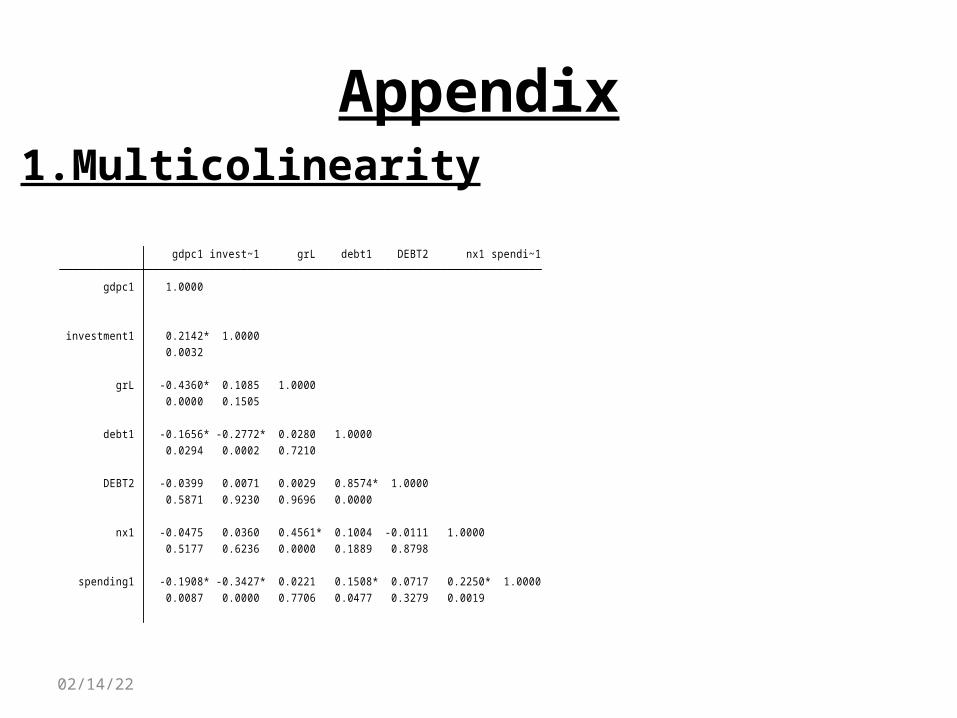
Appendix1.Multicolinearity

0.0087 0.0000 0.7706 0.0477 0.3279 0.0019 spending1 -0.1908* -0.3427* 0.0221 0.1508* 0.0717 0.2250* 1.0000 0.5177 0.6236 0.0000 0.1889 0.8798 nx1 -0.0475 0.0360 0.4561* 0.1004 -0.0111 1.0000 0.5871 0.9230 0.9696 0.0000 DEBT2 -0.0399 0.0071 0.0029 0.8574* 1.0000 0.0294 0.0002 0.7210 debt1 -0.1656* -0.2772* 0.0280 1.0000 0.0000 0.1505 grL -0.4360* 0.1085 1.0000 0.0032 investment1 0.2142* 1.0000 gdpc1 1.0000 gdpc1 invest~1 grL debt1 DEBT2 nx1 spendi~1

05/02/23

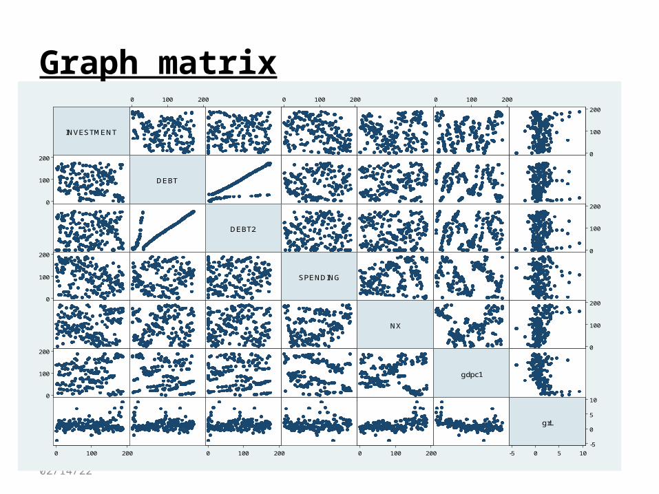
Graph matrix

INVESTMENT

DEBT

DEBT2

SPENDING

NX

gdpc1

grL

0

100

200

0 100 200

0

100

200

0 100 200

0

100

200

0 100 200

0

100

200

0 100 200

0

100

200

0 100 200

0

100

200

0 100 200

-5

0

5

10

-5 0 5 10

05/02/23

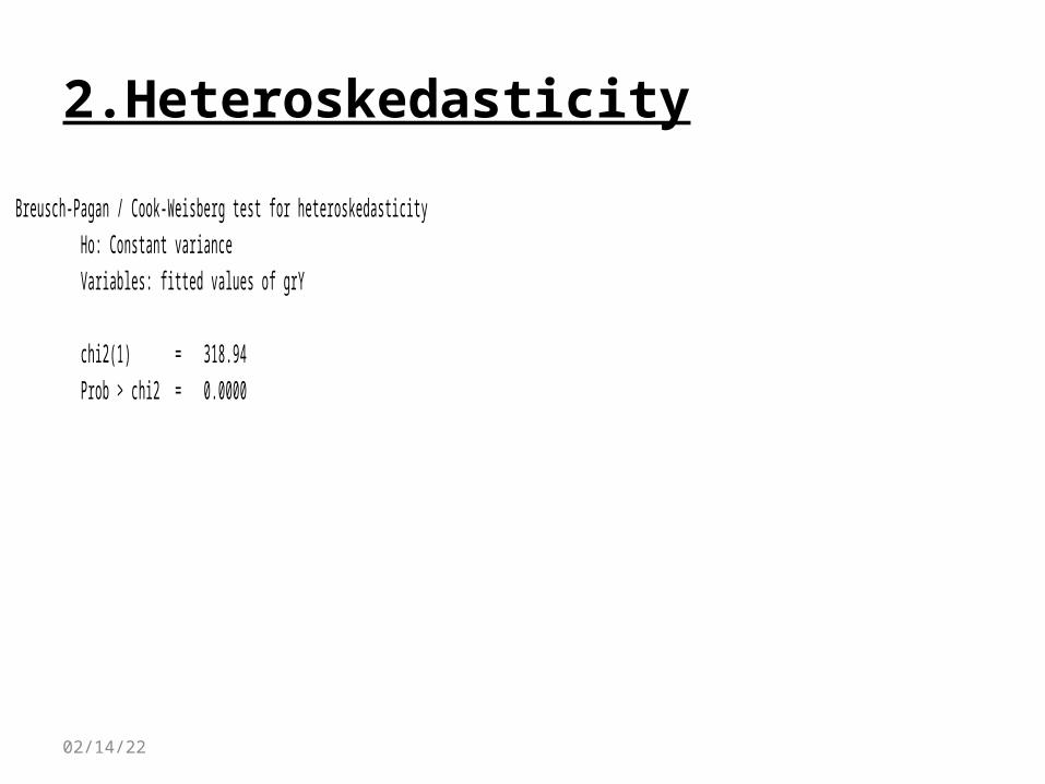
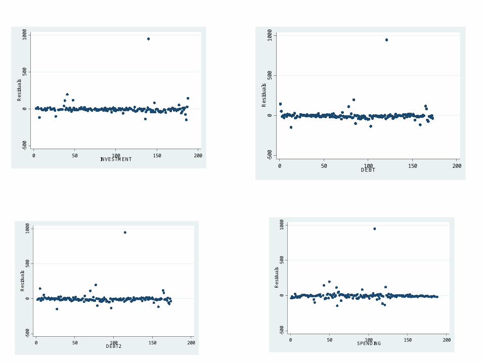
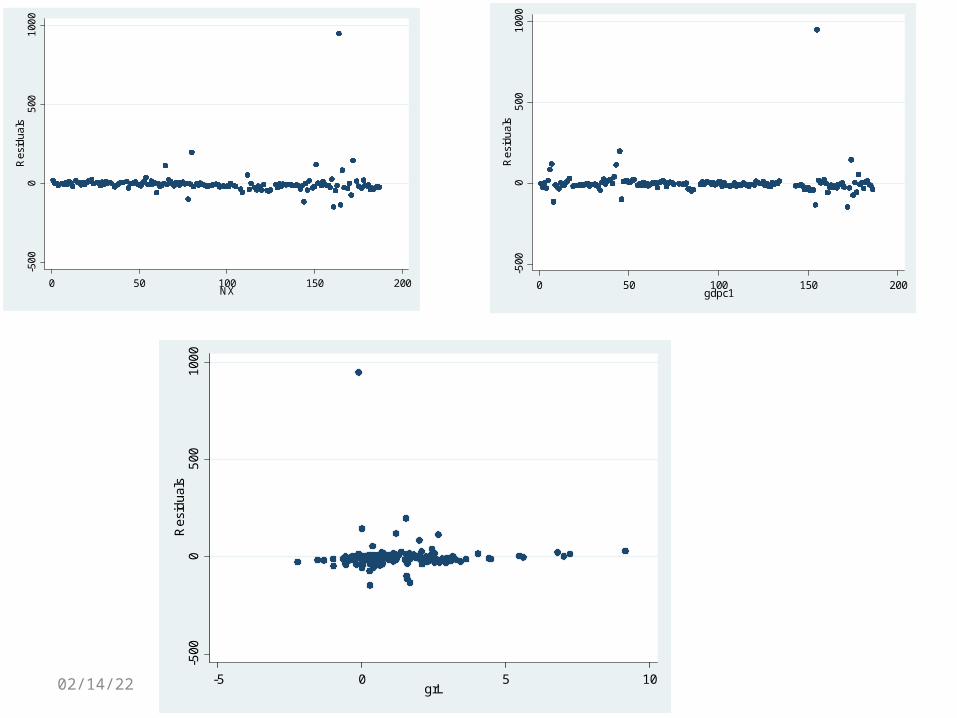
2.Heteroskedasticity

Prob > chi2 = 0.0000 chi2(1) = 318.94

Variables: fitted values of grY Ho: Constant varianceBreusch-Pagan / Cook-Weisberg test for heteroskedasticity

05/02/23

-500

050

010

00R

esid

uals

0 50 100 150 200INVESTMENT -5

000

500

1000

Res

idua

ls

0 50 100 150 200DEBT

-500

050

010

00R

esid

uals

0 50 100 150 200DEBT2

-500

050

010

00R

esid

uals

0 50 100 150 200 SPENDING

05/02/23

-500

050

010

00R

esid

uals

0 50 100 150 200NX

-500

050

010

00R

esid

uals

0 50 100 150 200gdpc1

-500

050

010

00R

esid

uals

-5 0 5 10grL

05/02/23

-500

050

010

00R

esid

uals

-500 0 500 1000Residuals, L

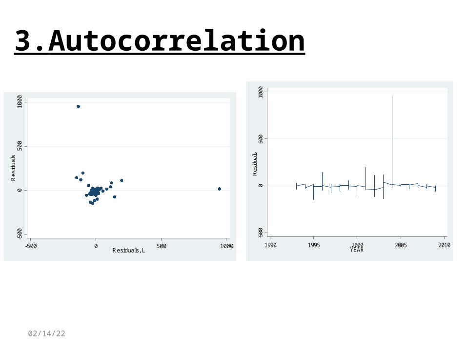
3.Autocorrelation

-500

050

010

00R

esid

uals

1990 1995 2000 2005 2010YEAR

05/02/23

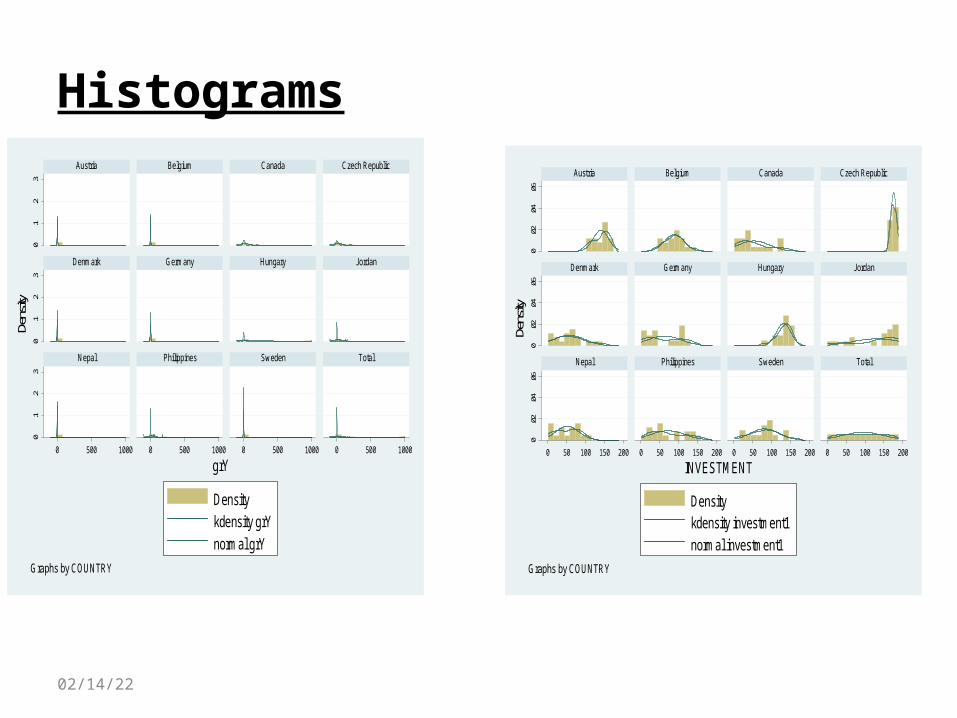
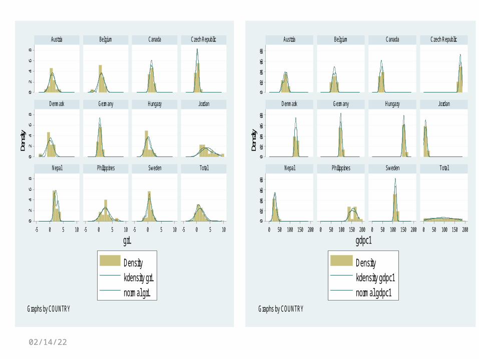
Histograms0

.1.2

.30

.1.2

.30

.1.2

.3

0 500 1000 0 500 1000 0 500 1000 0 500 1000



Nepal Philippines Sweden Total

Densitykdensity grYnormal grY

Den

sity

grY

Graphs by COUNTRY

0.0

2.0

4.0

60

.02

.04

.06

0.0

2.0

4.0

6

0 50 100 150 200 0 50 100 150 200 0 50 100 150 200 0 50 100 150 200




Densitykdensity investment1normal investment1

Den

sity

INVESTMENT

Graphs by COUNTRY

05/02/23

0.01

.02

.03

.04

0.01

.02

.03

.04

0.01

.02

.03

.04

0 50 100 150 200 0 50 100 150 200 0 50 100 150 200 0 50 100 150 200




Densitykdensity DEBT2normal DEBT2

Den

sity

DEBT2

Graphs by COUNTRY

0.0

2.0

4.0

60

.02

.04

.06

0.0

2.0

4.0

6

0 50 100 150 200 0 50 100 150 200 0 50 100 150 200 0 50 100 150 200




Densitykdensity debt1normal debt1

Den

sity

DEBT

Graphs by COUNTRY

05/02/23

0.05

0.05

0.05

0 50 100 150 200 0 50 100 150 200 0 50 100 150 200 0 50 100 150 200




Densitykdensity spending1normal spending1

Den

sity

SPENDING

Graphs by COUNTRY

0.02

.04

.06

0.02

.04

.06

0.02

.04

.06

0 50 100 150 200 0 50 100 150 200 0 50 100 150 200 0 50 100 150 200




Densitykdensity nx1normal nx1

Den

sity

NX

Graphs by COUNTRY

05/02/23

0.2

.4.6

.80

.2.4

.6.8

0.2

.4.6

.8

-5 0 5 10 -5 0 5 10 -5 0 5 10 -5 0 5 10




Densitykdensity grLnormal grL

Den

sity

grL

Graphs by COUNTRY

0.02

.04

.06

.08

0.02

.04

.06

.08

0.02

.04

.06

.08

0 50 100 150 200 0 50 100 150 200 0 50 100 150 200 0 50 100 150 200




Densitykdensity gdpc1normal gdpc1

Den

sity

gdpc1

Graphs by COUNTRY

05/02/23

050

01,00

00

500

1,00

00

500

1,00

0




grY

Graphs by COUNTRY

050

100

150

200

050

100

150

200

050

100

150

200




DEBT

Graphs by COUNTRY

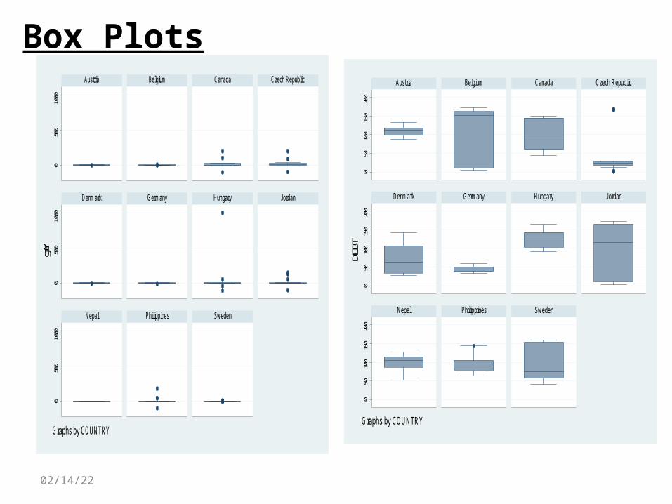
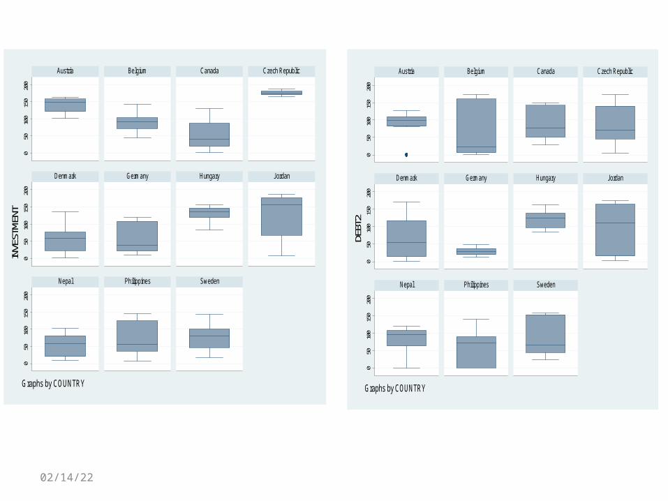
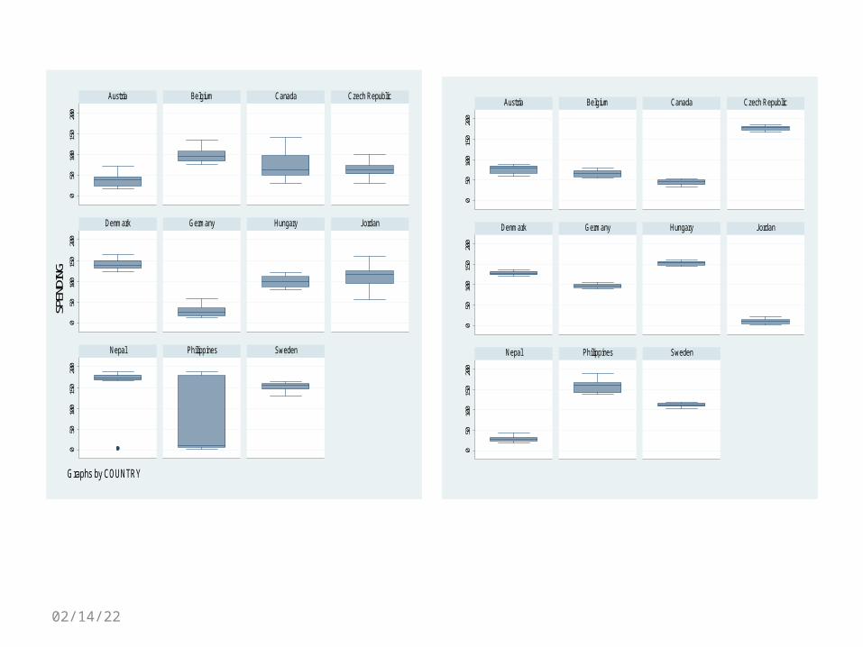
Box Plots

05/02/23

050

100

150

200

050

100

150

200

050

100

150

200




INVESTM

ENT

Graphs by COUNTRY

050

100

150

200

050

100

150

200

050

100

150

200




DEBT2

Graphs by COUNTRY

05/02/23

050

100

150

200

050

100

150

200

050

100

150

200




SPENDIN

G

Graphs by COUNTRY0

5010

015

020

00

5010

015

020

00

5010

015

020

0




05/02/23

050

100

150

200

050

100

150

200

050

100

150

200




NX

Graphs by COUNTRY-5

05

10-5

05

10-5

05

10




grL

Graphs by COUNTRY

05/02/23

050

010

00gr

Y

1990 1995 2000 2005 2010YEAR


050

100

150

200

DEBT

1990 1995 2000 2005 2010YEAR


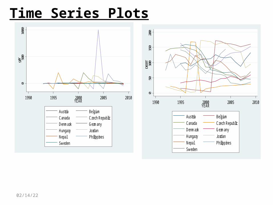
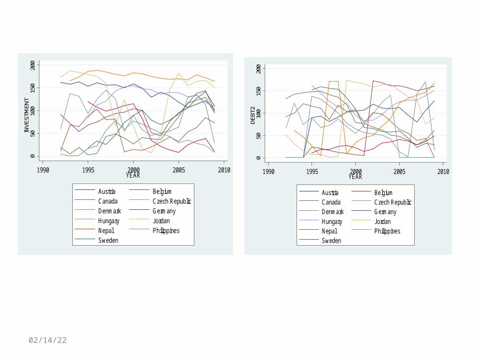
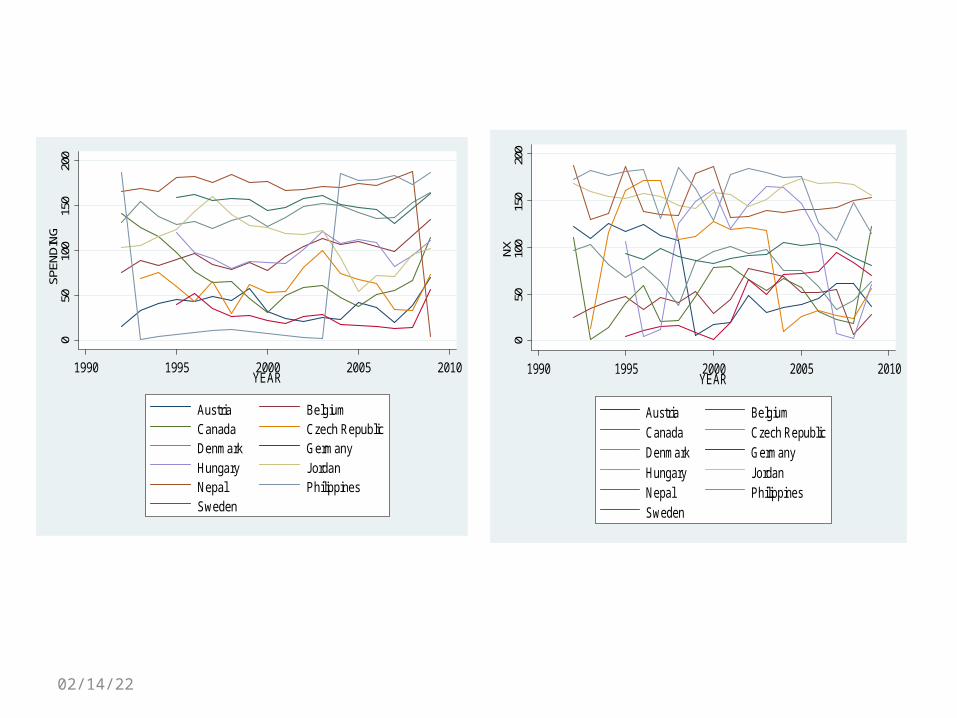
Time Series Plots

05/02/23

050

100

150

200

INVESTM

ENT

1990 1995 2000 2005 2010YEAR


050

100

150

200

DEBT2

1990 1995 2000 2005 2010YEAR


05/02/23

050

100

150

200

SPEN

DIN

G

1990 1995 2000 2005 2010YEAR


050

100

150

200

NX

1990 1995 2000 2005 2010YEAR


05/02/23

050

100

150

200

gdpc

1

1990 1995 2000 2005 2010YEAR


-50

510

grL

1990 1995 2000 2005 2010YEAR


05/02/23

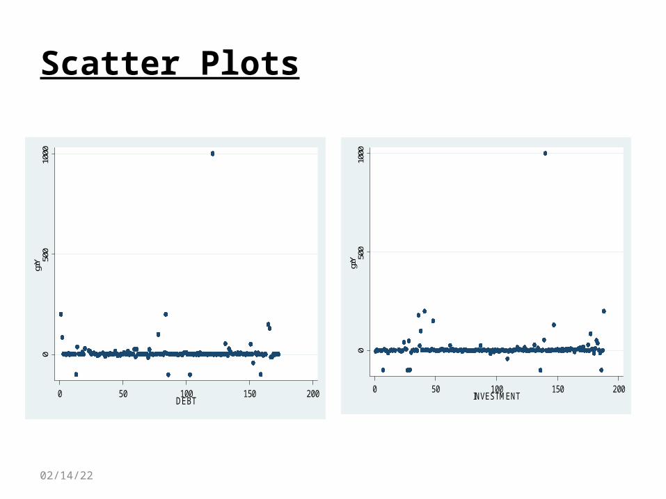
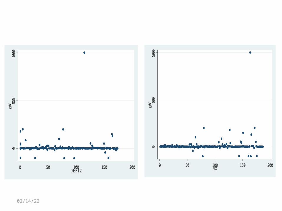
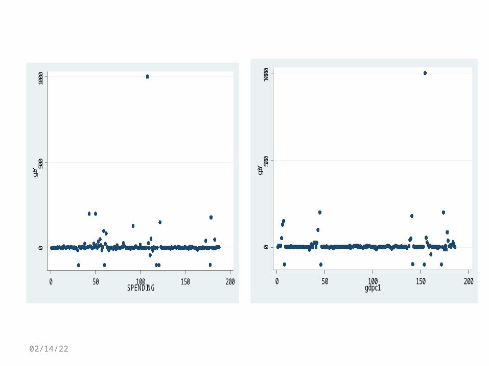
Scatter Plots0

500

1000

grY

0 50 100 150 200DEBT

050

010

00gr

Y

0 50 100 150 200INVESTMENT

05/02/23

050

010

00gr

Y

0 50 100 150 200DEBT2

050

010

00gr

Y

0 50 100 150 200NX

05/02/23

050

010

00gr

Y

0 50 100 150 200 SPENDING

050

010

00gr

Y

0 50 100 150 200gdpc1

05/02/23

050

010

00gr

Y

-5 0 5 10grL

05/02/23

OLS regression

_cons -15.3393 30.31154 -0.51 0.614 -75.21033 44.53173 spending1 -.0441388 .1402229 -0.31 0.753 -.3211056 .2328281 nx1 .2874147 .1522237 1.89 0.061 -.0132559 .5880853 DEBT2 -.0700736 .2819926 -0.25 0.804 -.6270623 .4869151 debt1 .1347734 .2947508 0.46 0.648 -.4474152 .7169619 grL -9.210227 5.576763 -1.65 0.101 -20.22539 1.804934 investment1 .1716439 .145282 1.18 0.239 -.1153156 .4586034 gdpc1 -.0521903 .1614234 -0.32 0.747 -.371032 .2666514 grY Coef. Std. Err. t P>|t| [95% Conf. Interval]

Total 1164430.82 164 7100.18792 Root MSE = 84.294 Adj R-squared = -0.0007 Residual 1115558.86 157 7105.47047 R-squared = 0.0420 Model 48871.9553 7 6981.7079 Prob > F = 0.4459 F( 7, 157) = 0.98 Source SS df MS Number of obs = 165

05/02/23

OLS ROBUST REGRESSION

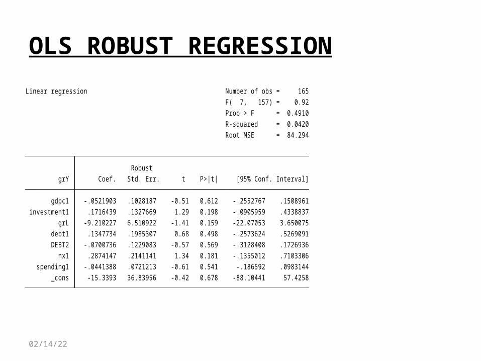
_cons -15.3393 36.83956 -0.42 0.678 -88.10441 57.4258 spending1 -.0441388 .0721213 -0.61 0.541 -.186592 .0983144 nx1 .2874147 .2141141 1.34 0.181 -.1355012 .7103306 DEBT2 -.0700736 .1229083 -0.57 0.569 -.3128408 .1726936 debt1 .1347734 .1985307 0.68 0.498 -.2573624 .5269091 grL -9.210227 6.510922 -1.41 0.159 -22.07053 3.650075 investment1 .1716439 .1327669 1.29 0.198 -.0905959 .4338837 gdpc1 -.0521903 .1028187 -0.51 0.612 -.2552767 .1508961 grY Coef. Std. Err. t P>|t| [95% Conf. Interval] Robust

Root MSE = 84.294 R-squared = 0.0420 Prob > F = 0.4910 F( 7, 157) = 0.92Linear regression Number of obs = 165

05/02/23

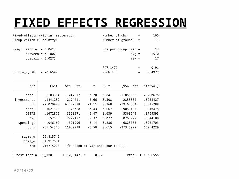
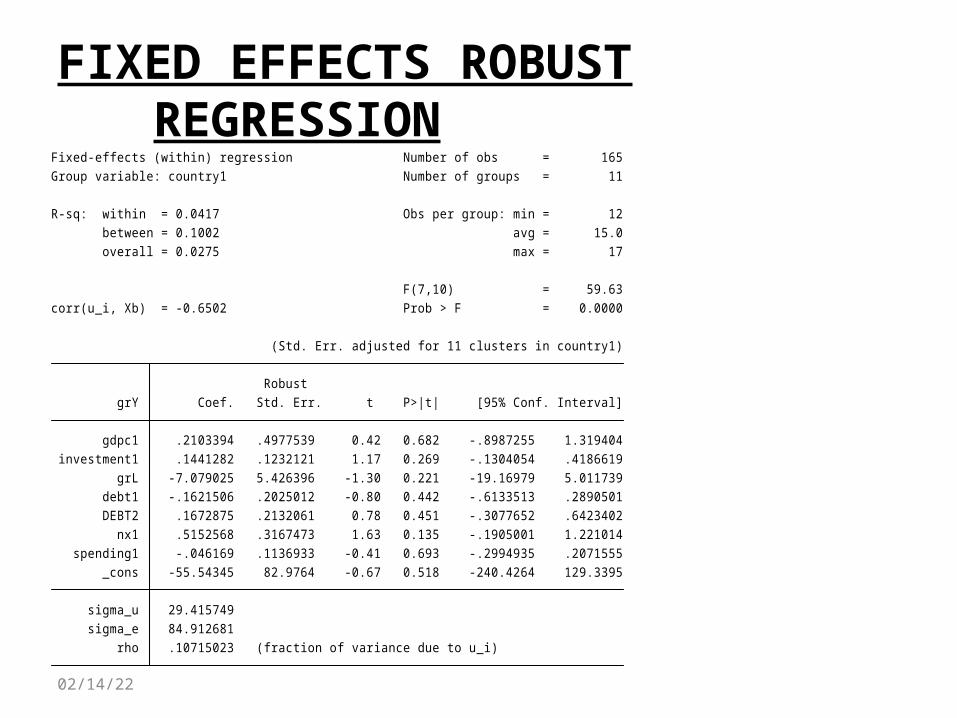
FIXED EFFECTS REGRESSION

F test that all u_i=0: F(10, 147) = 0.77 Prob > F = 0.6555 rho .10715023 (fraction of variance due to u_i) sigma_e 84.912681 sigma_u 29.415749 _cons -55.54345 110.2938 -0.50 0.615 -273.5097 162.4229 spending1 -.046169 .321996 -0.14 0.886 -.6825083 .5901703 nx1 .5152568 .2222177 2.32 0.022 .0761027 .9544108 DEBT2 .1672875 .3560571 0.47 0.639 -.5363645 .8709395 debt1 -.1621506 .376068 -0.43 0.667 -.9053487 .5810475 grL -7.079025 6.372888 -1.11 0.268 -19.67334 5.515288 investment1 .1441282 .2174411 0.66 0.508 -.2855862 .5738427 gdpc1 .2103394 1.047617 0.20 0.841 -1.859996 2.280675 grY Coef. Std. Err. t P>|t| [95% Conf. Interval]

corr(u_i, Xb) = -0.6502 Prob > F = 0.4972 F(7,147) = 0.91

overall = 0.0275 max = 17 between = 0.1002 avg = 15.0R-sq: within = 0.0417 Obs per group: min = 12

Group variable: country1 Number of groups = 11Fixed-effects (within) regression Number of obs = 165

05/02/23

FIXED EFFECTS ROBUST REGRESSION

rho .10715023 (fraction of variance due to u_i) sigma_e 84.912681 sigma_u 29.415749 _cons -55.54345 82.9764 -0.67 0.518 -240.4264 129.3395 spending1 -.046169 .1136933 -0.41 0.693 -.2994935 .2071555 nx1 .5152568 .3167473 1.63 0.135 -.1905001 1.221014 DEBT2 .1672875 .2132061 0.78 0.451 -.3077652 .6423402 debt1 -.1621506 .2025012 -0.80 0.442 -.6133513 .2890501 grL -7.079025 5.426396 -1.30 0.221 -19.16979 5.011739 investment1 .1441282 .1232121 1.17 0.269 -.1304054 .4186619 gdpc1 .2103394 .4977539 0.42 0.682 -.8987255 1.319404 grY Coef. Std. Err. t P>|t| [95% Conf. Interval] Robust (Std. Err. adjusted for 11 clusters in country1)

corr(u_i, Xb) = -0.6502 Prob > F = 0.0000 F(7,10) = 59.63


Group variable: country1 Number of groups = 11Fixed-effects (within) regression Number of obs = 165

05/02/23

RANDOM EFFECTS REGRESSION

rho .03090386 (fraction of variance due to u_i) sigma_e 84.912681 sigma_u 15.163361 _cons -15.63075 34.21572 -0.46 0.648 -82.69232 51.43083 spending1 -.0471542 .1594549 -0.30 0.767 -.3596799 .2653716 nx1 .3173845 .1610536 1.97 0.049 .0017253 .6330437 DEBT2 -.0347316 .2940462 -0.12 0.906 -.6110515 .5415883 debt1 .0800463 .3110469 0.26 0.797 -.5295944 .6896869 grL -9.051429 5.668779 -1.60 0.110 -20.16203 2.059173 investment1 .164416 .1572259 1.05 0.296 -.1437411 .4725731 gdpc1 -.0538993 .1838381 -0.29 0.769 -.4142153 .3064168 grY Coef. Std. Err. z P>|z| [95% Conf. Interval]

corr(u_i, X) = 0 (assumed) Prob > chi2 = 0.4907 Wald chi2(7) = 6.43


Group variable: country1 Number of groups = 11Random-effects GLS regression Number of obs = 165

05/02/23

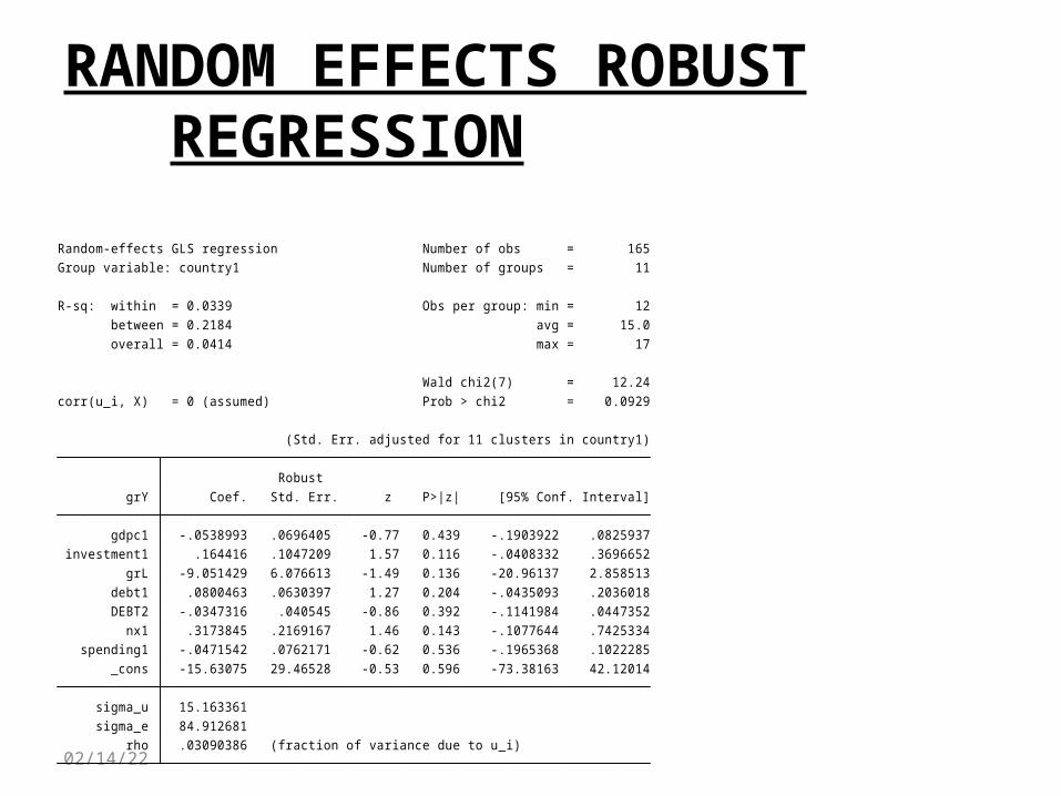
RANDOM EFFECTS ROBUST REGRESSION

rho .03090386 (fraction of variance due to u_i) sigma_e 84.912681 sigma_u 15.163361 _cons -15.63075 29.46528 -0.53 0.596 -73.38163 42.12014 spending1 -.0471542 .0762171 -0.62 0.536 -.1965368 .1022285 nx1 .3173845 .2169167 1.46 0.143 -.1077644 .7425334 DEBT2 -.0347316 .040545 -0.86 0.392 -.1141984 .0447352 debt1 .0800463 .0630397 1.27 0.204 -.0435093 .2036018 grL -9.051429 6.076613 -1.49 0.136 -20.96137 2.858513 investment1 .164416 .1047209 1.57 0.116 -.0408332 .3696652 gdpc1 -.0538993 .0696405 -0.77 0.439 -.1903922 .0825937 grY Coef. Std. Err. z P>|z| [95% Conf. Interval] Robust (Std. Err. adjusted for 11 clusters in country1)

corr(u_i, X) = 0 (assumed) Prob > chi2 = 0.0929 Wald chi2(7) = 12.24


Group variable: country1 Number of groups = 11Random-effects GLS regression Number of obs = 165

05/02/23

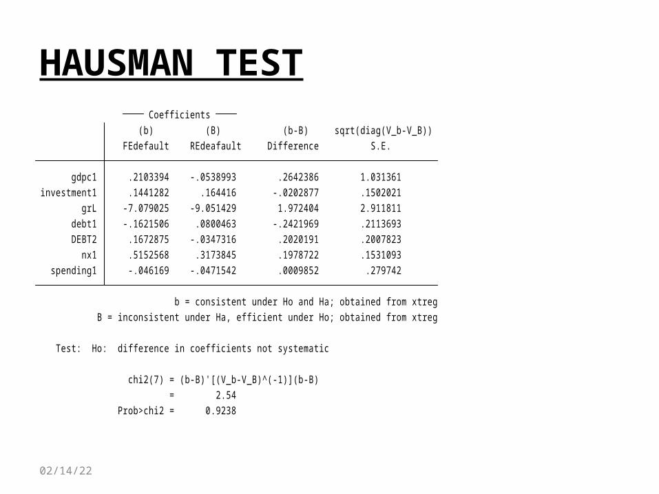
HAUSMAN TEST

Prob>chi2 = 0.9238 = 2.54 chi2(7) = (b-B)'[(V_b-V_B)^(-1)](b-B)

Test: Ho: difference in coefficients not systematic

B = inconsistent under Ha, efficient under Ho; obtained from xtreg b = consistent under Ho and Ha; obtained from xtreg spending1 -.046169 -.0471542 .0009852 .279742 nx1 .5152568 .3173845 .1978722 .1531093 DEBT2 .1672875 -.0347316 .2020191 .2007823 debt1 -.1621506 .0800463 -.2421969 .2113693 grL -7.079025 -9.051429 1.972404 2.911811 investment1 .1441282 .164416 -.0202877 .1502021 gdpc1 .2103394 -.0538993 .2642386 1.031361 FEdefault REdeafault Difference S.E. (b) (B) (b-B) sqrt(diag(V_b-V_B)) Coefficients

05/02/23

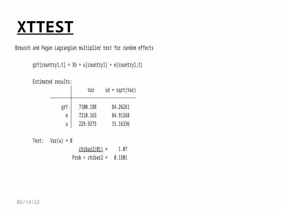
XTTEST

Prob > chibar2 = 0.1501 chibar2(01) = 1.07 Test: Var(u) = 0

u 229.9275 15.16336 e 7210.163 84.91268 grY 7100.188 84.26261 Var sd = sqrt(Var) Estimated results:

grY[country1,t] = Xb + u[country1] + e[country1,t]

Breusch and Pagan Lagrangian multiplier test for random effects

05/02/23

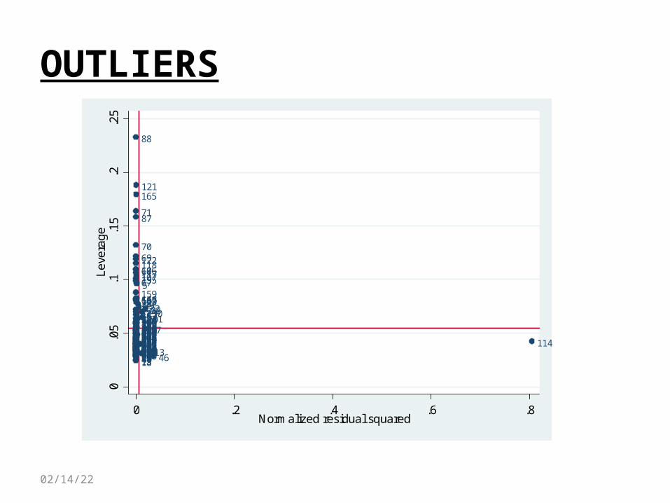
OUTLIERS

4

5

67

8910111213

1415161718222324252627

28

293031323334

35

363839404142434445

46474849505152535456

57

5859

60

6162636465

66

67686970

71

75

76777879808182838485

86

87

88

89

919293949596979899100101102103104

106107

108109110111112113114

115116

117118

119

121

122

123124125126127128129

130131132

133

134

135

136137

139140141142143144

145146147148149150151152153154157158

159

160161

162163

164

165

166167

168175176177178179180181182183184185186187188

0.0

5.1

.15

.2.2

5Le

vera

ge

0 .2 .4 .6 .8Normalized residual squared

05/02/23

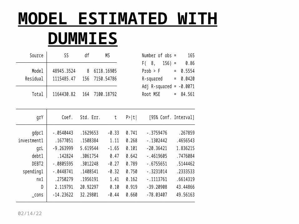
MODEL ESTIMATED WITH DUMMIES

_cons -14.23622 32.29801 -0.44 0.660 -78.03407 49.56163 D 2.119791 20.92297 0.10 0.919 -39.20908 43.44866 nx1 .2750279 .1956191 1.41 0.162 -.1113761 .6614319 spending1 -.0448741 .1408541 -0.32 0.750 -.3231014 .2333533 DEBT2 -.0805595 .3012248 -0.27 0.789 -.6755651 .5144462 debt1 .142824 .3061754 0.47 0.642 -.4619605 .7476084 grL -9.263999 5.619544 -1.65 0.101 -20.36421 1.836215 investment1 .1677051 .1508384 1.11 0.268 -.1302442 .4656543 gdpc1 -.0540443 .1629653 -0.33 0.741 -.3759476 .267859 grY Coef. Std. Err. t P>|t| [95% Conf. Interval]


05/02/23

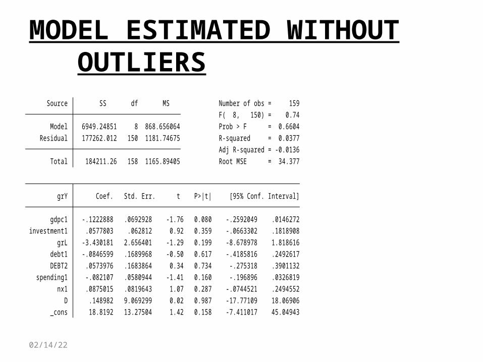
MODEL ESTIMATED WITHOUT OUTLIERS

_cons 18.8192 13.27504 1.42 0.158 -7.411017 45.04943 D .148982 9.069299 0.02 0.987 -17.77109 18.06906 nx1 .0875015 .0819643 1.07 0.287 -.0744521 .2494552 spending1 -.082107 .0580944 -1.41 0.160 -.196896 .0326819 DEBT2 .0573976 .1683864 0.34 0.734 -.275318 .3901132 debt1 -.0846599 .1689968 -0.50 0.617 -.4185816 .2492617 grL -3.430181 2.656401 -1.29 0.199 -8.678978 1.818616 investment1 .0577803 .062812 0.92 0.359 -.0663302 .1818908 gdpc1 -.1222888 .0692928 -1.76 0.080 -.2592049 .0146272 grY Coef. Std. Err. t P>|t| [95% Conf. Interval]


Download - An empirical investigation of economic growth and debt

Top Related