
07-036
Copyright © 2006, 2007, 2008 by Noel H. Watson
Working papers are in draft form. This working paper is distributed for purposes of comment and discussion only. It may not be reproduced without permission of the copyright holder. Copies of working papers are available from the author.
A Perceptions Framework for Categorizing Inventory Policies in Single-stage Inventory Systems Noel H. Watson

A Perceptions Framework for Categorizing Inventory Policies inSingle-stage Inventory Systems
Noel Watson
Harvard Business School, Soldiers Field Road, Boston, MA 02163
July 31, 2008
In this paper we propose a perceptions framework for categorizing a range of inventory decisionmaking that can be employed in a single-stage supply chain. We take the existence of a wide rangeof inventory decision making processes, as given and strive not to model the reasons that the rangepersists but seek a way to categorize them via their effects on inventory levels, orders placed giventhe demand faced by the inventory system. Using a perspective that we consider natural and thusappealing, the categorization involves the use of conceptual perceptions of demand to underpinthe link across three features of the inventory system: inventory levels, orders placed and actualdemand faced. The perceptions framework is based on forecasting with Auto-Regressive IntegratedMoving Average (ARIMA) time series models. The context in which we develop this perceptionsframework is of a single stage stochastic inventory system with periodic review, constant leadtimes,infinite supply, full backlogging, linear holding and penalty costs and no ordering costs. Forecast-ing ARIMA time series requires tracking forecast errors (interpolating) and using these forecasterrors and past demand realizations to predict future demand (extrapolating). So called optimalinventory policies are categorized here by perceptions of demand that align with reality. Naturallythen, deviations from optimal inventory policies are characterized by allowing the perception aboutdemand implied by the interpolations or extrapolations to be primarily different from the actualdemand process. Extrapolations and interpolations being separate activities, can in addition, implydiffering perceptions from each other and this can further categorize inventory decision making.
1 Introduction
In this paper we propose a perceptions framework for categorizing a range of inventory decision
making in a single-stage supply chain. The perceptions framework is based on forecasting with
Auto-Regressive Integrated Moving Average (ARIMA) time series models. In this paper, we take
the existence of a wide range of inventory decision making processes as given and strive not to model
the reasons that the range persists but seek a way to categorize them via their effects on inventory
levels, orders placed given the demand faced by the inventory system. Using a perspective that we
consider natural and thus appealing, the categorization involves the use of conceptual perceptions
of demand to underpin the link across three features of the inventory system: inventory levels,
orders placed and actual demand faced. With limited emphasis on the cost consequences of the
1

inventory policies, (sake in the distinction of optimal and suboptimal,) our categorization is less an
economics-based one, but rather process-based, focusing instead on the stochastic processes that
characterize the inventory levels, orders and demand levels at the inventory system and how they
can be considered inter-related. We also examine the implications of our inventory decision making
categories with respect to the variance and uncertainty of these stochastic processes, characteristics
which we expect would have significant influence on the costs for an inventory system and for its
supply chain.
Our use of the term perception is motivated by its use in organizational behavior theory on
organizational decision making, March and Simon (1993), Cyert and March (1992). In such theory,
perception of reality in terms of environment, decision alternatives, goals or consequences of actions
are considered significant drivers of decision making. These perceptions can be misaligned with
reality (assuming an objective assessment of this reality) since they are considered the outcome of
psychological, sociological and operational processes with their attendant strengths and weaknesses.
Why do we need such a framework? In the operations literature, the assumption of the com-
pletely rational agent has dominated the research surrounding inventory policies. However devi-
ations from the optimal policy are prevalent in practice and analytical models to understand the
effects of inventory dynamics on practice may require means of modeling them. Modeling devi-
ations from optimal policy can also augment our understanding of inventory systems and supply
chains, in a manner akin to sensitivity analysis in mathematical programming, as the dynamics
surrounding optimal management of these systems may not completely describe these systems. For
example, although the optimal EOQ is determined via strict optimization of standard setup and
holding costs, the inventory cost function is well-known to be fairly “flat” around this point.
Inventory decision making, in addition to being influenced by the above mentioned perceptions
of reality, will also be the outcome of a combination of psychological, sociological, organizational
and operational processes, Oliva and Watson (2004, 2007). We refer to a particular combination
of perceptions and decision making processes as an inventory decision making setting. In order to
categorize these settings, we make the strong assumption that such settings can be grouped based
on the inventory levels, orders and demand persistently exhibited within the system, despite these
settings being otherwise considered different from each other. For example, when the operations
literature has assumed a rational agent for particular inventory decisions say in response to i.i.d.
demand, we would infer a reference to all settings where the particular combination of perceptions
and decision making processes results in processes for inventory levels and orders along with de-
mand that resemble rational behavior. In this paper, the commonality used for grouping settings
2

is represented by stochastic processes, serving as conceptual perceptions of demand. These per-
ceptions form both a conceptual and a satisfying analytic link between inventory levels and orders
placed and the actual demand faced by the inventory. The details of this analytic link and thus
the particular operationalization of our perceptions framework make use of the ARIMA time series
models, Box et. al. (1994).
From Box et. al., forecasting ARIMA time series requires tracking forecast errors (interpolating)
and using these forecast errors and past demand realizations to predict future demand (extrapo-
lating). Both interpolation and extrapolation are actions that can be considered to imply a belief
about the demand process or a perception, as they are based on a particular time series demand
model when performed by a completely rational agent. So called optimal inventory policies are
categorized here by perceptions of demand that align with reality. Naturally then, categorizing
deviation from optimal inventory policies is possible if we allow that the time series used for in-
terpolating or extrapolating, that is, what we interpret as a belief about the demand process or
perception, may not be the same as the actual demand process. Further deviations can even be
categorized by allowing that the perception implied by interpolations do not match those implied
by extrapolations.
In this paper, we establish these conceptual perceptions as analytic links connecting inventory
levels or orders and the actual demand. In so doing, we also provide a prediction for the effects
of a range of inventory decision making settings on inventory levels and orders. For example, we
can suggest the effects of inventory decision making that ignore any non-stationary properties of
demand. In an effort to further our appreciation of the framework, we interpret simple forecasting
techniques used for inventory policies such as the moving average and exponential smoothing using
our framework. Interestingly we show that in order to categorize the use of the moving average, we
need slightly different perceptions in interpolation versus that of extrapolation justifying the need
for the framework’s flexibility. In an effort to improve our understanding of the effects of suboptimal
policies on the process characteristics of inventory levels and orders, we also examine separately, the
effects of misaligned perceptions along the autoregressive and then the moving average dimensions
of the ARIMA modeled demand process and focus on the implications for variance and uncertainty
of the inventory and order processes. Given that these are the two critical dimensions of the
ARIMA processes which model our perceptions, understanding how each dimension separately
affects inventory levels and orders should help our understanding of their effects in tandem.
The use of ARIMA processes as the foundation for this perceptions framework is motivated by
the following two important observations: First as cited in Gaur et. al. real-life demand patterns
3

often follow higher-order autoregressive processes due to the presence of seasonality and business
cycles. For example, the monthly demand for a seasonal item can be an AR(12) process. More
general ARMA processes are found to fit demand for long lifecycle goods such as fuel, food products,
machine tools, etc., as observed in Chopra and Meindl (2001) and Nahmias (1993). Second, the
results in this paper along with recent research show that ARMA demand processes occur naturally
in multistage supply chains. For example, Zhang (2004) studied the time-series characterization
of the order process for a decision maker serving ARMA demand and using a periodic-review
order-up-to policy. They show an “ARMA-in-ARMA-out” principle for perceptions aligned with
actual demand, i.e., if demand follows an ARMA(p, q) process, then the order process is an ARMA
(p,max [p, q − l]) process, where l is the replenishment lead time. Gilbert (2005) extended these
results to ARIMA process but still for aligned perceptions. We find a similar ”ARIMA-in-ARIMA-
out” principle for orders given a wider range of inventory policies. Such a result increases our
expectations for the prevalence of these processes in real world supply chains.
It needs to be pointed out that in our framework we do not use perception in its more con-
ventional sense. We are not making any claims about the actual perception of any manager in
this paper and how decisions are made by these managers. However, there are real world scenar-
ios which resemble details of our perception framework more closely than others. One scenario
involves fitting ARIMA stochastic models to historical demand data, Gooijer (1985), Koreisha
and Yoshimoto (1991). Different methods for fitting these stochastic processes including the Box-
Jenkins approach, the corner method and extended sample autocorrelations, have been shown to
have varying performance in correctly identifying these processes. Poor identification then could
result in a situation where the demand process used for inventory management is misaligned with
reality. A second scenario involves subjective forecasting. Lawrence and O’Connor (1992) in a fore-
casting study investigate the extent to which some of the widely documented judgemental biases
and heuristics apply to time series forecasting. The time series used were modeled from stationary
ARMA processes. The authors found that subjects’ forecasts could be modeled as an AR(1) process
that was not always aligned with actual.
Supply chain issues which we expect could benefit from our framework include the bullwhip
effect and its mitigation Lee, et. al. (1997), value of information sharing in a supply chain, Lee, et.
al. (2000), Cachon and Fisher (2000), Raghunathan (2001), Gaur et. al. (2005) and the general
coordination of a supply chain whether via incentives Cachon (2000) or more structural approaches
such as leadtime reduction, Cachon and Fisher, or network rationalization. For example, in section
4.2, we make some comments on the value of sharing information in a supply chain. In Watson and
4

Zheng (2005), misaligned perceptions implying deviations from optimal inventory policies, were
also used to test the robustness of decentralization schemes for serial supply chains, that is, how
well the schemes mitigated the resulting increase in total systems costs.
Section 2 presents the general demand model and inventory system while Section 3 introduces
the perceptions framework within the context of optimal inventory management. Section 4 con-
tinues the introduction but within the context of suboptimal inventory policies focusing, for sake
of simplicity, on true demand modeled as stationary ARMA stochastic processes. Section 5 exam-
ines misaligned perceptions along the autoregressive and moving average dimensions separately. In
Section 6 we also examine policies based on simple forecasting techniques. Section 7 completes the
presentation of the perceptions framework within the context of suboptimal inventory policies with
a treatment of demand modeled as non-stationary ARIMA processes.
2 The Demand Model and Inventory System
In this paper, we use the general class of Auto-Regressive Integrated Moving Average (ARIMA)
time-series models to model both demand and perceptions of demand. In this section we describe
the methodology for forecasting with these time series models once they have been specified. Since
perceptions are also modeled as ARIMA time series models, the description is applicable for un-
derstanding the details of the mechanics of the perceptions framework.
We follow the notation of Box et. al. (1994). Stationary demand will be represented by an
autoregressive moving average model, ARMA(p, q) with p the number of autoregressive terms and
q the number of moving average terms:
Zt = µ+ φ1 (Zt−1 − µ) + φ2 (Zt−2 − µ) + ...+ φp (Zt−p − µ) + at − θ1at−1 − θ2at−2 − ...− θqat−q
(1)
= µ+
pXi=1
φi (Zt−i − µ) + at +qXi=1
−θiat−i,
where Zt is the demand at time, µ is the level or mean of demand and at is a noise series of
independent identically distributed random variables with mean 0 and variance σ2a.
The ARMA models can be represented more concisely and are more easily manipulated math-
ematically by using a backshift operator. Let B denote the time-series backshift operator such
that
BZt = Zt−1 and BnZt = Zt−n.
5

The above stationary series (1) can be written using the backshift operator as follows:
φ (B) (Zt − µ) = θ (B) at,
where φ (B) = 1− φ1B − φ2B2 − ...− φpB
p and is referred to as the autoregressive operator with
order p, and θ (B) = 1−θ1B−θ2B2− ...−θqBq which is referred to as the moving average operator
with order q.
Non-stationary demand can be modeled by assuming that some differencing results in a station-
ary ARMA series. ∇ will be used to denote the difference operation such that ∇Zt = (1−B)Ztand ∇dZt = (1−B)d Zt where ∇d = (1−B)d is the polynomial resulting from raising 1−B to the
dth power. Assuming the dth difference of a non-stationary demand series is stationary, the series
can be represented by an autoregressive integrated moving average or ARIMA(p, d, q) series:
φ (B)∇dZt = θ (B) at (2)
or
ϕ (B)Zt = θ (B) at,
where ϕ (B) = φ (B)∇d is a polynomial of order p+ d and is referred to as the generalized autore-
gressive operator .
2.1 ARIMA(p, d, q) Forms and Forecasting
There are three different “explicit” forms for the general model (2) . The current value of Zt can
be expressed:
1. In terms of the realizations of previous Zt−j : j > 0 and current and previous realizations
at−j , j = 0, 1, ... as implied by (2) :
(Zt − µ) = (1− ϕ (B)) (Zt−1 − µ) + θ (B) at.
2. In terms of the current and previous realizations at−j , j = 0, 1, .... This representation is seen
by rewriting (2) as follows
(Zt − µ) = ψ (B) at, (3)
where ψ (B) = 1 +P∞j=1 ψjB
j = θ (B) /ϕ (B) . In particular:
ψj = ϕp+dψj−p−d + ...+ ϕ1ψj−1 − θj : j > 0
6

where ψ0 = 1, ψj = 0 for j < 0, and θj = 0 for j > q. For the ARMA time series, the stationary
property is guaranteed if the series ψ (B) is infinitely summable, that is, ifP∞j=1 |ψj | < ∞.
For an ARIMA time series Zt, although ∇dZt is stationary, Zt is not. Therefore the infinite
sum (3) above, is not summable and so does not converge in any sense. Alternatively we
can rewrite (18) in terms of the dth difference which does have a converging sum of random
shocks. As a notational device, for ARIMA time series we will refer to this infinite random
shock form to represent the infinite random shock form of the dth difference.
3. In terms of the realizations of previous Zt−j and current at. This representation is seen by
rewriting (2) as follows
π (B) (Zt − µ) = at,
where π (B) = 1−P∞j=1 πjB
j = ϕ (B) /θ (B) . This implies the following
(Zt − µ) =∞Xj=1
πj (Zt−j − µ) + at.
In particular:
πj = θqπj−q + ...+ θ1πj−1 + φj : j > 0
where π0 = −1, πj = 0 for j < 0 and φj = 0 for j > p. An invertibility property for (2) implies
that this is a legitimate form. The property is guaranteed by restricting the series π (B) to
be infinitely summable, that is,P∞j=1 |πj | <∞. This property can hold for stationary ARMA
as well as non-stationary ARIMA time series.
These three forms can be used for forecasting Zt once the model of demand process has been
estimated or specified and are equivalent, i.e., the forecast is the same independent of which fore-
casting form is used. We show that their effect on inventory systems are not always equivalent for
perceptions that are not aligned with reality.
2.2 The Inventory System
The inventory context in which we develop the perceptions framework is the following. We assume
an inventory system managed by a retailer with periodic review and constant leadtime L, infinite
supply, full backlogging, linear holding and penalty costs, no ordering costs and infinite history.
Demand is assumed to follow an ARIMA process (2) with d ≥ 0 satisfying the stationary property
but not necessarily the invertibility property. The sequence of operations in a period are that 1)
there is receipt of inventory previously ordered 2) demand arrives within a period and is met from
7

on-hand inventory, and then 3) orders are placed. Let It be the inventory at the retailer at the end
of period t. Consistent with the assumptions on the costs of the inventory system, we will assume
an order up-to policy for the retailer with target st for period t.Where necessary we allow costless
returns which implies that orders from the retailer in period t are given by
Ot = Zt + st+1 − st. (4)
The primary purpose of this paper is to examine the use of perceptions as a framework for
categorizing inventory policies, therefore we will for simplicity and brevity assume that the inventory
system has zero leadtime, that is, L = 0. The results for arbitrary leadtime have similar themes.
3 The Perceptions Framework Applied to Optimal Inventory Poli-cies
In this section we introduce the perceptions framework within the context of optimal inventory
management.
3.1 Aligned Perceptions: Optimal Inventory policies.
Consider the general demand process for the retailer (2) and the optimal inventory policy for
minimizing expected single period costs which, in this setting, is the myopic order up-to policy.
For this optimal policy, at the end of period t − 1, the retailer calculates the forecast Zt−1 which
minimizes the forecast error for period t and combines this forecast with a constant safety stock
T . From Box et. al. as mentioned earlier this forecast can be generated using any of the three
explicit forms of the demand process. The first two forms require, however, the retailer to calculate
at least the most recent random shock at−1. This is calculated as the difference between the actual
realization and the one period ahead forecast, that is, at−1 = Zt−1 − Zt−2 for an ARMA time
series or at−1 = ∇dZt−1 −∇dZt−2 for an ARIMA time series. (Here ∇dZt−2 serves as convenient
notation for the forecasted dth difference.) When our retailer calculates the difference between the
actual realization and the one period ahead forecast, she interpolates the realizations of the unseen
random shocks. When the retailer makes her forecast Zt−1 using any of the explicit forms, she is
extrapolating, that is, using previous realizations and interpolations to predict future realizations.
Both interpolation and extrapolation as actions can be considered to imply a belief about the
demand process as they are based on a particular time series model. We attribute this time series
implied by either forecasting operation of interpolation or extrapolation as a perception about the
demand process. The resulting optimal forecasts and inventory policies can then be considered
8

optimal partly because the perception of the retailer, that is, the belief of the demand process,
is aligned (or matches) with the actual demand process. The terms introduced here, perception,
interpolation and extrapolation will be used in the next section for categorizing a wider range of
inventory policies beyond the optimal policy for an inventory system.
The theorems below characterize the stochastic process for the inventory levels at the retailer
and her orders assuming the myopic policy described above and comes from Gilbert. These results
will be compared with those obtained when we examine the perceptions framework within a context
of misaligned perceptions of demand.
Theorem 3.1 An aligned perception is associated with a time series of inventory It which is
ARIMA(0,0,1) with the form It − T = aIt where aIt = −at.
Theorem 3.2 An aligned perception is associated with a time series of orders Ot which is
ARIMA¡p, d, qO
¢with the form
ϕ (B) (Ot − µ) = θO (B) aOt
where aO = KOat, θO (B) = θ(B)−ϕ(B)
BKO + ϕ(B)KO , q
O = max (p+ d, q − 1) and KO = 1 + ϕ1 − θ1.
Proposition 3.3 For stationary ARMA demand process, the variance of the time series (Ot − µ)
is greater than that of (Zt − µ) if and only if φ1 − θ1 > 0.
3.2 Discussion of Optimal Policy
Theorem 3.1 suggests that inventory would rarely follow a process more complex than a simple
i.i.d. process despite the complexity of the demand process and further, that the mean of this
inventory process is equal to the intended safety stock T. Theorem 3.2 shows that the optimal
orders follow an ARIMA process similar to that of demand except for differences in the variance of
the random shock and in the moving average operator of the process. The random shock for the
order process has variance¡KOσa
¢2= (1 + ϕ1 − θ1)
2 σ2a. In Gilbert and Watson and Zheng (2008)
the coefficient |KO| is interpreted as an alternative measure of the bullwhip effect complementing
the more conventional measure of the ratio of variance of orders to demand. Watson and Zheng
refer to the coefficient |KO| as the bullwhip effect modulo full information and interpret it as the
best case increase (or decrease) in uncertainty for a potential supplier given full distributional
knowledge about demand and knowledge about the inventory policy of the retailer. The greater
the coefficient |KO|, the greater the expected uncertainty for the supplier despite her extensive
9

information. Proposition 3.3 shows that for aligned perceptions, this bullwhip effect modulo full
information is consistent with the traditional measure of the bullwhip effect.
The results for aligned perceptions here provide added argument for the need for a framework on
deviations from the optimal policy. Theorem 3.1 provides very strict expectations for the inventories
of a retailer, (that it follows a ARIMA (0,0,1) process,) which we would be surprised, if we found
completely characterized a majority of inventory systems.
3.3 Formalizing Framework Concepts: Perceptions, Interpolations and Extrap-olations
We assimilate the concepts of perception, interpolation and extrapolation introduced in the previous
subsections within a context of forecasting with ARIMA time series models in order to provide
our framework. Perception we will define as the implied characterization of the demand process
facing the inventory system. Conceptually, perceptions can be implied from interpolations and
extrapolations. In this paper, interpolation is the action of inferring past but hidden realizations,
in this case, the unseen random shock from demand realizations. Extrapolation is the action
of using historical realizations and/or interpolations to predict future demand realizations. In
order to impute a characterization of demand, that is, a perception, from an action requires an
explicit mapping of demand processes to actions. Our mapping corresponds to that generated by a
completely rational agent making forecasts for a given ARIMA demand specification. In essence, a
perception is implied from an interpolation or extrapolation by assuming the action to be performed
by a completely rational agent and then inferring the demand process which drives the action. By
our definition of perception, it will not be necessary for the perception imputed from interpolations
to be the same with that imputed from extrapolations (as implicitly assumed in the optimal policy
above) even though the implicit assumption is that the actions (and perceptions) categorize the
same inventory system. More importantly neither of these perceptions need be aligned with reality.
Using the above introduced definitions, we can examine a range of inventory policy responses by
our retailer and study the effects on her orders and inventory levels.
4 Perceptions Framework for Suboptimal policies: Misaligned Sta-tionary Perceptions
In this section we move beyond optimal policies and begin to examine inventory decision mak-
ing that can be termed suboptimal. In our framework, such policies are categorized by percep-
tions which do not align with reality and thus we will term them misaligned perceptions. In this
10

section we will concentrate on stationary demand processes and stationary perceptions, that is,
ARMA (ARIMA with d = 0) processes as in (1) , while in Section 7 we focus on non-stationary
ARIMA (d > 0) demand processes. Our categorization will be based on two perceptions, one for
interpolations and one for extrapolations. Therefore we can consider two variations in the extent
of the misaligned perceptions. The first (section 4.2) considers the same misaligned perceptions in
both extrapolations and interpolations and the second considers different perceptions for extrapola-
tions and interpolations. Although the first variation concerns perceptions that could be described
as internally consistent since that used for extrapolation matches that used for interpolations, the
second variation follows from recognizing that these perceptions do not have to be so. In section
4.3 we consider one example where the perception used for interpolation is different from that used
for extrapolation. In particular we consider misaligned perceptions in extrapolations but aligned
perceptions in interpolations. Furthermore, in section 6, we interpret the use of the moving av-
erage and exponential smoothing using our perceptions framework. The example of the moving
average policy considered in section 6.1 will serve as another example where the perception used
for interpolation will be different from the perception used for extrapolation. Our main goal in this
section (and paper) is to establish these perceptions as the fundamental component of an analytic
link between the demand process and the process for inventory levels and orders. In so doing, we
also provide a prediction for the effects of “suboptimal” inventory decision making on inventory
levels and orders.
4.1 Misaligned Stationary Perceptions : ARMA(p, q) processes
In this subsection we discuss the general stationary perceptions that can be attributed to inter-
polations and extrapolations which we will allow to differ from the actual demand process. All
stationary and invertible ARMA processes can serve as misaligned perceptions, thus follow an
ARMA(p, q) process:
φ (B) (Zt − µ) = θ (B) at (5)
where φ (B) = 1− φ1B− φ2B2− ...− φpBp, θ (B) = 1− θ1B− θ2B2− ...− θqBq, and at is a random
noise series with mean 0 and variance σa. The stationary and invertible properties from section 2.1
are assumed to hold and thus all three explicit forms of forecasting will be legitimate. In (5) it is
possible for p = p, q = q, µ = µ, φj = φj , θj = θj for some j or σa = σa.
We will assume that the forecasts for extrapolations are denoted by Zet [k] which specifically
denotes the forecast of demand at time t + k made at time t after demand is observed. Since we
concentrate on zero leadtimes, we only deal with single period ahead forecasts, Zet [1] , which we
11

will denote Zet . Recall from section 2.1 that there are three different explicit forms for the general
ARIMA models and that these forms imply three different approaches to calculating Zet . We will
denote these three forms as Zet (1), Zet (2) and Z
et (3) which coincide sequentially with the three
explicit forms from Section 2.1 and define them explicitly as follows:
Zet (1) = µ+1− φ (B)
B(Zt − µ) +
θ (B)− 1B
at, (6)
Zet (2) = µ+ψ (B)− 1
Bat, (7)
Zet (3) = µ+1− π (B)
B(Zt − µ) , (8)
where ψ (B) = θ (B) /φ (B) and π (B) = φ (B) /θ (B) . The above formulas are generated by taking
the expectation at time t of demand in period t+ 1, Zt+1, using the three explicit forms listed in
Section 2.1 for the process (5). Note that at time t, Eat+1 = 0. Furthermore the realizations ak,
k ≤ t, are determined from interpolations. Note finally that Zet (3) does not use any interpolations.
For interpolations, recall that it is the difference between the actual realization and the one
period ahead forecast that is used to generate the realization for the demand shock at that are used
for extrapolations in (6) and (7) above. We let Zit denote this one period ahead forecast based
on the perceptions used for the interpolation. As with extrapolation, we can denote three forms
for Zit as Zit (1), Z
it (2) and Z
it (3) which again coincide sequentially with the three explicit forms
listed in Section 2.1. Specifically at = (Zt − µ) −³Zit−1 (J)− µ
´where the forecast used in the
interpolation could be of any of the three forms J = 1, 2, 3. For J = 3, is it is easy to show that we
can then write at = π (B) (Zt − µ) where π (B) = φ (B) /θ (B) . Note that since the perception (5)
is invertible, π (B) is legitimate. Note that the other two forms J = 1, 2 also make use of demand
realizations determined from prior interpolations. For these forms it only takes a little more work
to show that we still get at = π (B) (Zt − µ) . We write this as a proposition:
Proposition 4.1 For misaligned interpolations, either form of the single period ahead forecast
Zit (J) , J = 1, 2, 3, results in realization of demand shocks which can be formulated as at =
π (B) (Zt − µ) where π (B) = φ (B) /θ (B) .
4.2 Consistent Misaligned Perceptions in Interpolation and Extrapolation
In this subsection by characterizing the stochastic processes for the inventory levels and orders
given the same misaligned perception in both interpolations and extrapolations, we establish this
perception as the basis for the link between the process characteristics of the system. After the
12

results provided below we describe the more interesting relationships between the categorizing
perception and the process results.
Assume without loss of generality that this misaligned perception is defined as the ARMA(p, q)
process (5) . We have the following theorems:
Theorem 4.2 A misaligned perception attributed to both interpolation and extrapolation is associ-
ated with a time series of inventory It which is ARMA¡pI , qI
¢is with the form
φI (B)³It − T I
´= θI (B) aIt
and:aIt = K
Iat pI = q + p θI (B) = −φ(B)θ(B)KI
KI = −1 qI = p+ q
T I = T +³1−B−π(B)
B
´(µ− µ) φI (B) = φ (B) θ (B)
This time series is stationary and independent of the explicit forecasting form used for either
interpolation or extrapolation. The time series is also invertible if the demand process is invertible.
Theorem 4.3 A misaligned perception attributed to both interpolation and extrapolation is associ-
ated with a time series of orders Ot which is ARMA¡pO, qO
¢with the form
φO (B)³Ot − µ
´= θO (B) aOt
and:aOt = K
Oat pO = p+ q θO (B) =³θ(B)−φ(B)(1−B)
BKO
´θ (B)
KO = 1 + φ1 − θ1 qO = max (p+ q, q + q − 1)φO (B) = θ (B)φ (B)
This time series is stationary and independent of the explicit form used for either interpolation
or extrapolation but not necessarily invertible.
Perceptions Perspective on the Inventory Level Process: Theorem 4.2 above shows that
the inventory level process for a misaligned perception in both interpolations and extrapolations
is not i.i.d. (versus results for aligned perception in Theorem 3.1) but can follow a wide range of
ARMA processes. The inventory level process is driven by both the perception and the demand
process. In particular, the autoregressive and moving average operators from both the perception
and the demand process determine the operators of the inventory level process. Furthermore, since
T I = T +³1−B−π(B)
B
´(µ− µ) , a perception which has mean µ 6= µ results in essentially a different
safety factor as the mean of the inventory level process. Here notice that except for the mean of
actual demand, this safety factor is completely determined by the perception and is independent
13

of the stochastic process for actual demand. As expected this safety factor T I is usually lower
than T if µ ≥ µ since³1−B−π(B)
B
´tends to be negative (since -1 is the constant in the polynomial³
1−B−π(B)B
´,) however this relation does not have to hold.
Perceptions Perspective on the Order Process: As with the inventory level process,
the order process is determined by the perception and the demand process. This is an important
observation given its relationship to supply chain research on sharing demand for improving supply
chain coordination, e.g., Lee, So and Tang. Researchers have argued that sharing such demand
would help supply chain coordination in three ways: 1) historical demand information would help
upstream stages forecast end-customer demand more accurately, which would then improve the
forecasts of future orders from downstream stages, 2) knowing real-time demand realizations would
also improve accuracy of forecasts of future orders, Lee, So and Tang, and 3) end-customer demand
can prove a more robust guide for orders placed by upstream partners than their incoming orders,
Watson and Zheng (2005). Our perceptions perspective here speak to the first two arguments. To
the first argument, our results suggest that for improving forecasts of orders, an understanding of
the demand process needs to be complemented by an understanding of the inventory policy of the
downstream stage creating the orders. Historically, these orders have been assumed to come from
aligned perceptions with the demand process, but if in reality these perceptions are not aligned,
then forecasting demand is not sufficient for forecasting incoming orders. In particular, we see in
Theorem 4.3 that the bullwhip effect modulo information for orders |KO|, that is the uncertainty
inherent in orders, is related only to the parameters of the misaligned perception and not to that of
the actual demand process. With respect to the second argument, the results suggest interestingly
that sharing current demand realizations does not improve accuracy of order forecasts since the
order process is also ARMA and thus completely characterized by previous orders and interpolated
errors in forecasting, see Raghunathan (2001) for similar finding with aligned perceptions.
4.3 Inconsistent Misaligned Perceptions in Extrapolation and Interpolation
In this subsection we continue our examination of inventory decision making that can be termed
suboptimal, focusing on those which are categorized by differing perceptions in extrapolations
versus interpolations. We will consider a simple example of this variation where the perceptions
from extrapolations are not aligned with the actual demand process (1), while the perceptions
from interpolations are so aligned. This variation is considered to be one example but not the
only such example where the perception used for interpolation is different from that used for
extrapolation. Our results show that allowing perceptions to differ between interpolations and
14

extrapolations, allows us to categorize a larger range of inventory decision making settings than
when the perceptions are not allowed to differ. The example of the moving average policy considered
in section 6.1 will serve as an example where the perception used for interpolation will be different
from the perception used for extrapolation.
First consider interpolations. Since the perceptions here is of a belief that matches with reality,
we assume that the one period ahead forecasts used here, Zit , are equal to those of the completely
rational agent, that is, Zit = Zt. This gives generated realizations for the random shocks, which will
be used in extrapolation, that match with reality, i.e., at = at.
Now consider extrapolations. Assume w.l.o.g. that the misaligned perception attributed to our
extrapolation follows the ARMA(p, q) process (5) . For clarity, we write below the three explicit
forms of the one period ahead forecasts:
Zet (1) = µ+1− φ (B)
B(Zt − µ) +
θ (B)− 1B
at; (9)
Zet (2) = µ+ψ (B)− 1
Bat; (10)
Zet (3) = µ+1− π (B)
B(Zt − µ) ; (11)
Note that in the first two explicit forms of Zet we use the random shock terms at instead of at to
reflect interpolations with aligned perceptions.
The following are theorems characterizing the inventory levels and orders from our retailer for
the first and second explicit forecasting form. Note that since the third explicit forecasting form
is the same here as when extrapolations and interpolations are both misaligned, the results in
theorems 4.2 and 4.3 apply in that case. The first difference to note between the results here and
in section 4.2 is that here for inconsistent misaligned perceptions, the form of forecasting affects
the results for inventory and orders, whereas for consistent misaligned perceptions in section 4.2,
it does not.
Theorem 4.4 A misaligned perception in extrapolation only and where extrapolations use the first
explicit form of forecasts, is associated with a time series of inventory It which is ARMA¡p, qI
¢with the form
φ (B) (It − T I) = θI (B) aIt
and:aIt = K
Iat qI = max {p+ q − 1, p+ q, p+ q}KI = −(1 + φ1 − φ1) θI (B) = 1
KI
³φ(B)−φ(B)
B θ (B) + φ(B)³θ (B)− 1− θ (B)
´´T I = T +
³1−B−φ(B)
B
´(µ− µ)
15

and associated with a time series of orders Ot which is ARMA¡p, qO
¢with the form
φ (B)³Ot − µ
´= θO (B) aOt
and:aOt = K
Oat qO = max {p+ q, p+ q}KO = 1 + φ1 − θ1 θO (B) = 1
KO
³θ(B)B −
³φ (B)
³θ (B)− 1
´− θ (B) φ (B)
´(1−B)B
´Both time series It and Ot are stationary but not necessarily invertible.
Theorem 4.5 A misaligned perception in extrapolations only and where extrapolations use the
second explicit form of forecasts, is associated with a time series of inventory It which is ARMA¡pI , qI
¢with the form
φI (B) (It − T I) = θI (B) aIt
and:aIt = K
Iat qI = max {p+ q, q + p, p+ p}KI = −1 θI (B) = 1
KI
³θ (B)φ (B)− θ (B) φ (B)− φ (B)φ (B)
´T I = T − (µ− µ)pI = p+ p φI (B) = φ (B)φ (B)
and associated with a time series of orders Ot which is ARMA¡pO, qO
¢with the form
φO (B)³Ot − µ
´= θO (B) aOt
and:aOt = K
Oat qO = max {p+ q, q + p, p+ p}KO = 1 + φ1 − θ1 θO (B) = 1
KO θ (B) φ (B) +θ(B)−φ(B)
B φ (B) (1−B)pO = p+ p φO (B) = φ (B)φ (B)
Both time series It and Ot are stationary but not necessarily invertible.
Theorems 4.4 and 4.5 above show that the resulting processes for inventory and orders depend
on which form of forecasting is used. For example, inventory and orders under the first form of fore-
casting in Theorem 4.4 have the same autoregressive operator as the demand process while under
the second form, in Theorem 4.5, the autoregressive operator for inventory and orders can be quite
different from actual demand, i.e., φ (B) 6= φI (B) and φ (B) 6= φO (B). Comparing Theorems 4.4
and 4.5 for inconsistent misaligned perceptions with Theorems 4.2 and 4.3 for consistent misaligned
perceptions further shows how the inventory and order processes can differ when the perceptions
are not consistent. For example, the variational coefficient KI in the inventory model in Theorem
4.4 is rarely equal to -1 for inconsistent misaligned perceptions while it is always equal to -1 in The-
orem 4.2. Furthermore inconsistent misaligned perceptions can result in inventory level processes
16

that are not invertible while consistent misaligned perceptions always result in invertible inventory
level processes if the demand process is invertible. This implies that allowing the perceptions for
interpolations and extrapolations to differ from each other can help categorize a greater range of
inventory decision making settings than when the perceptions are confined to be the same.
5 Investigating the Effects of Consistent Misaligned Perceptionsalong Auto-Regressive and Moving Average Dimensions
In an effort to improve our understanding of the effects of suboptimal policies on the process
characteristics of inventory levels and orders, and promote the utility of our perceptions framework,
we examine perceptions where the misalignment is either along the autoregressive dimension or
moving average dimension but not both. Given that these are the two critical dimensions of the
ARIMA processes which model our perceptions, understanding how each dimension separately
affects inventory levels and orders should help our understanding of their effects in tandem. We
will refer to these misalignments as autoregressive based misalignments and moving average based
misalignments respectively and restrict our attention to consistent misaligned perceptions. We will
examine the implications of both types of misalignment with respect to the variance and uncertainty
of the inventory level and order processes.
5.1 Auto-regressive based Misalignments
In this subsection we consider misaligned perceptions with the misalignment along the autore-
gressive dimension. Given that demand follows the ARMA process (1), an autoregressive based
misaligned perception is the following ARMA(p, q) process
φ (B) (Zt − µ) = θ (B) at (12)
where φ (B) = 1− φ1B − φ2B2 − ...− φpB
p. Note that we assume that the mean of perception is
the same as that of actual demand. The following proposition will be used to discuss this type of
misalignment.
Proposition 5.1 An autoregressive based misaligned perception in both the interpolation and ex-
trapolation is associated with a time series of inventory It which is ARMA¡p, qI
¢is with the form
φ (B) (It − T ) = θI (B) aIt
and:
17

aIt = KIat KI = −1 qI = p θI (B) =
³− φ(B)
KI
´and associated with a time series of orders Ot which is ARMA
¡p, qO
¢with the form
φ (B) (Ot − µ) = θO (B) aOt
and:
aOt = KOat qO = max (p, q − 1) KO = 1 + φ1 − θ1 θO (B) = θ(B)
BKO − φ(B)(1−B)BKO
These inventory and order time series are independent of the explicit form used for either
interpolations or extrapolations.
Perception Perspective on the Inventory Level Process: Comparing results for aligned
perceptions from Theorem 3.1 with results for autoregressive based misalignments from Proposition
5.1, we see that an autoregressive based misalignment introduces an autoregressive operator into the
inventory level process which is the same as that of the demand process. Recall that under aligned
perceptions, the inventory level process was i.i.d. A moving average operator is also introduced
into the inventory level process. As expected, in Proposition 5.2, we show that aligned perceptions
result in the lowest variance for the inventory process.
Proposition 5.2 If φ (B) 6= φ (B) then³It − T
´has a larger variance than (It − T ) .
Monotonic results for changes in variance of inventory with changes in parameters of the mis-
aligned perception depend on the parameters of actual demand. In Proposition 5.3 below when the
coefficients of the autoregressive operator for actual demand are all positive and either all greater
than or less than those of the misaligned perception, then variance will increase with the divergence
of the misaligned perception from that of actual demand. Such monotonic properties do not always
hold however for example, if some of the autoregressive coefficients are negative.
Proposition 5.3 Assume p ≤ p and φi ≥ 0, for all i, if φi − φi ≥ 0 for all i or φi − φi ≤ 0 for all
i, then the variance of It is increasing in¯φi − φi
¯for all i.
Perception Perspective on the Order Process: Comparing results for aligned perceptions
from Theorem 3.2 with results for autoregressive based misalignment from Proposition 5.1, we see
an autoregressive based misalignment does not change the autoregressive operator of the order
process from what would have resulted from an aligned perception. Furthermore, the bullwhip
effect modulo full information, that is the uncertainty inherent in orders, is determined by the
18

mis-estimate of the first coefficient of the autoregressive operator φ1. When φ1 ≥ φ1, this implies
that the bullwhip effect modulo full information is greater than for aligned perceptions, else lower.
With respect to the variance of orders, Proposition 5.4 provides monotonic results for changes in the
coefficients of the autoregressive operator of the perception. We find that given positive coefficients
in the autoregressive operator of demand, the variance of orders increases as the coefficients of the
autoregressive operator of the perception increase. The assumption in the proposition that ψi for
i ≥ 1 is a decreasing sequence is not too onerous due to the assumption of the stationarity property
but it does mean that ψi ≥ 0 for all i.
Proposition 5.4 Given Ot − µ = ψ (B) aot , assume that the sequence ψi for i ≥ 1 is a decreasing
sequence. If φi ≥ 0 for all i, then for all i, V ar³Ot − µ
´increases as φi increases.
5.2 Moving Average based Misalignments
In this subsection we consider misaligned perceptions with the misalignment along the moving
average dimension. Given that demand follows the ARMA process (1), a moving average based
misaligned perception is the following ARMA(p, q) process
φ (B) (Zt − µ) = θ (B) at. (13)
where θ (B) = 1− θ1B− θ2B2− ...− θqB
q. Note that we again assume that the mean of perception
is the same as that of actual demand.
Proposition 5.5 A moving average based misalignment in both the interpolation and extrapolation
is associated with a time series of inventory It which is ARMA¡pI , q
¢is with the form
φI (B) (It − T ) = θ (B) aIt
and:aIt = K
Iat pI = q φI (B) = 1KI
³−θ (B)
´KI = −1and associated with a time series of orders Ot which is ARMA
¡pO, qO
¢with the form
φO (B) (Ot − µ) = θO (B) aOt
and:aOt = K
Oat pO = q + p φO (B) = φ (B) θ (B)
KO = 1 + φ1 − θ1 qO = max (p+ q, q + q − 1) θO (B) =³
θ(B)BKO − φ(B)(1−B)
BKO
´θ (B)
This order time series is independent of the explicit form used for either interpolations or
extrapolations.
19

Perceptions Perspective on the Inventory Level Process: Comparing the results for
aligned perceptions in Theorem 3.1 with the results for moving average based misalignments in
Proposition 5.5, we see that a moving average based misalignment introduces a moving average
operator to the inventory process which is the same as that of the demand process. Recall again
that under aligned perceptions, the inventory level process was i.i.d. An autoregressive operator
is also introduced into the inventory process since pI = q. As expected, from Proposition 5.6
below, misaligned perceptions increase the variance of the inventory level process versus aligned
perceptions.
Proposition 5.6 If θ (B) 6= θ (B) then³It − T
´has a larger variance than (It − T ) .
As with autoregressive based misalignments, monotonic results for changes in variance of inven-
tory with changes in parameters of the misaligned perception depend on the parameters of actual
demand. In Proposition 5.7 below, when the coefficients of the moving average operator of the per-
ception are all positive and either all greater than or less than those of the demand, then variance
will increase with the divergence of the misaligned perception from that of actual demand. Such
monotonic properties do not always hold however for example, if some of all of the moving average
coefficients in the misaligned perception are negative.
Proposition 5.7 Assume q ≤ q and θi ≥ 0, for all i, if θi − θi ≥ 0 for all i or θi − θi ≤ 0 for all
i, then the variance of It is increasing in¯θi − θi
¯for all i.
Perception Perspective on the Order Process: Comparing the results for aligned percep-
tions in Theorem 3.2 with the results for moving average based misalignments in Proposition 5.5,
we see that a moving average based misalignment has an effect on both the autoregressive and on
the moving average dimensions of the order process compared to aligned perceptions. The bull-
whip effect modulo full information is determined by the mis-estimate of the first moving average
coefficient θ1. If θ1 ≥ θ1 then the uncertainty surrounding orders is less than that for aligned per-
ceptions, else greater. With respect to the variance of orders we are unable to prove monotonicity
results for changes in the parameters of the misaligned perception. Rather, Proposition 5.8 pro-
vides monotonic results for changes in the coefficients of the moving average operator of the actual
demand holding the moving average operator of the misaligned perception constant. (This is the
reverse of our findings for the autoregressive based alignments above, justifying somewhat the need
for separating the analysis along the two dimensions as we do here.) We find that given positive
coefficients in the moving average operator of perception, the variance of orders increases as the
20

coefficients of the moving average operator of the demand increase. Again the assumption that
ψi for i ≥ 1 is a decreasing sequence is not too onerous due to the assumption of the stationarity
property but it does mean that ψi ≥ 0 for all i.
Proposition 5.8 Given Ot − µ = ψ (B) aot , assume that the sequence ψi for i ≥ 1 is a decreasing
sequence. If θi ≥ 0 for all i, then for all i, Ot − µ increases as θi increases.
6 Perceptions Perspective on Moving Average Forecasting andExponential Smoothing
In this section we will see how simple forecasting approaches such as the moving average and
exponential smoothing can be examined using the perceptions framework. The main goal will be
to describe the perceptions that could be attributed to the use of these forecasting approaches. For
completeness, the predictions on the stochastic processes for inventory levels and orders are also
provided.
6.1 Moving Average Forecasting
The moving average involves the use of the simple average of the previous n demand realizations,
Znt as an estimate of the mean of the demand process. Here
Znt =
Pni=1 Zt−i+1n
.
Forecast errors for the moving average are calculated as Znt−i − Zt−i+1 for all i and the simple
average of the previous n forecast errors, σnt is also used as an estimate of the standard deviation of
the forecast error and used to determine a proxy for the safety stock of the inventory policy. Here
σnt =
Pni=1
¡Znt−i − Zt−i+1
¢n
. (14)
The order up-to target for the inventory system is Znt + σnt k with σnt k as the implied safety factor.
Here the estimate of the mean of the demand process and the safety factor comprise the order-up-to
target, implying that our safety stock T = 0. This results in the following claim for inconsistent
misaligned perceptions which categorize the use of the moving average for setting inventory policies.
The claim follows since it directly mimics the use of the moving average just described and lemmas
6.1 and 6.2 show the perceptions to be stationary and invertible.
21

Claim 1 The perceptions implied by the use of an order up-to target Znt + σnt k is of the following
ARMA(n, 0) process for interpolations:
φ (B) (Zt − µ) = at
where φ (B) = 1−Pni=1
1nB
i and the following ARMA(n, n) process for extrapolations:
φ (B) (Zt − µ) = θ (B) at
where θ (B) = 1−Pni=1
−kn B
i, and φ (B) = φ (B) .
Lemma 6.1 The time series
φ (B) (Zt − µ) = at
where φ (B) = 1−Pni=1
1nB
i is stationary and invertible.
Lemma 6.2 The time series
φ (B) (Zt − µ) = θ (B) at
where θ (B) = 1−Pni=1
−kn B
i, and φ (B) = φ (B) is stationary and invertible.
Note here that the mean of the demand process assumed in the perception is the same as
actual since the moving average is used intuitively to estimate the actual level rather than assume
a preconceived one. The explicit form of forecasting used for either interpolation or extrapolation
here is the first explicit form, that is, J = 1. The perception implied by interpolations matches
with how forecast errors are calculated for the moving average, thus note that it is an ARMA
(n, 0) process. The perception implied by extrapolation matches with how inventory targets are
set, thus note that the moving average dimension of this perception calculates the simple average
of the previous n forecast errors and then combines it with the safety factor k. For completeness
we provide the results for inventory levels and orders that are associated with the perceptions in
Claim 1, given that demand follows the ARMA process (1).
Proposition 6.3 The use of the moving average of the n previous demand realizations for an order
up-to Znt + σnt k inventory policy is associated with a time series of inventory It which is ARMA¡p, qI
¢with the form
φ (B) It = θI (B) aIt
and:
22
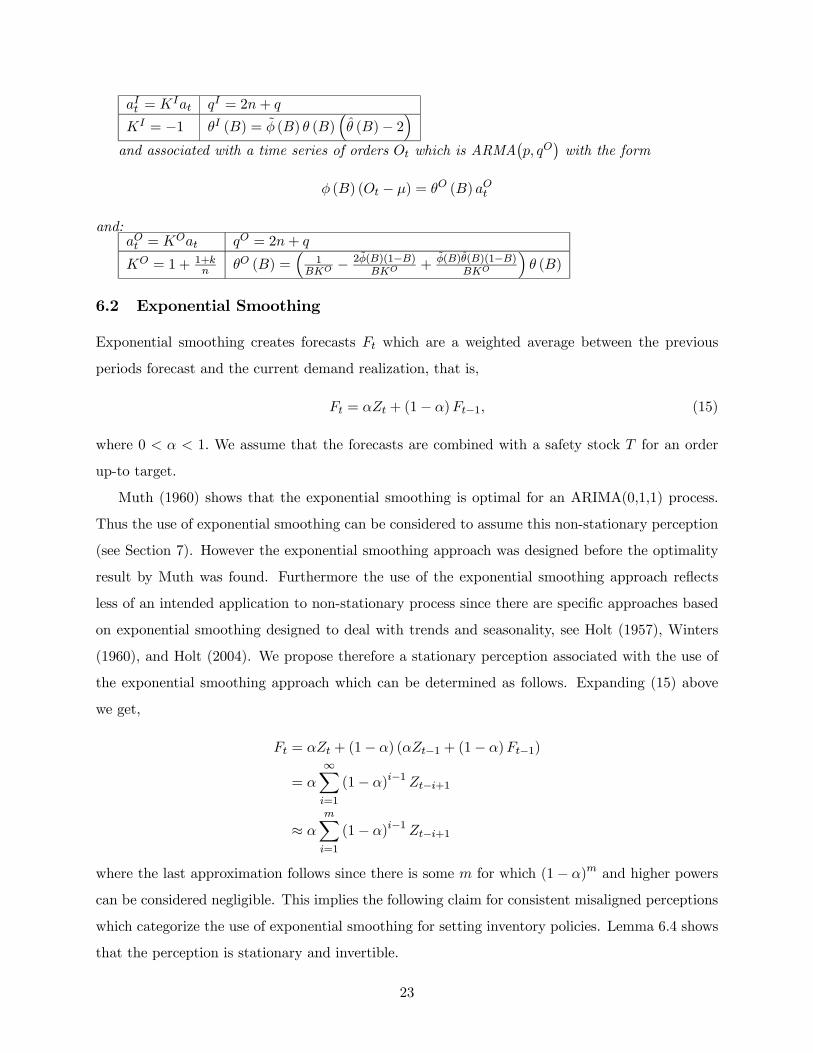
aIt = KIat qI = 2n+ q
KI = −1 θI (B) = φ (B) θ (B)³θ (B)− 2
´and associated with a time series of orders Ot which is ARMA
¡p, qO
¢with the form
φ (B) (Ot − µ) = θO (B) aOt
and:aOt = K
Oat qO = 2n+ q
KO = 1 + 1+kn θO (B) =
³1
BKO − 2φ(B)(1−B)BKO + φ(B)θ(B)(1−B)
BKO
´θ (B)
6.2 Exponential Smoothing
Exponential smoothing creates forecasts Ft which are a weighted average between the previous
periods forecast and the current demand realization, that is,
Ft = αZt + (1− α)Ft−1, (15)
where 0 < α < 1. We assume that the forecasts are combined with a safety stock T for an order
up-to target.
Muth (1960) shows that the exponential smoothing is optimal for an ARIMA(0,1,1) process.
Thus the use of exponential smoothing can be considered to assume this non-stationary perception
(see Section 7). However the exponential smoothing approach was designed before the optimality
result by Muth was found. Furthermore the use of the exponential smoothing approach reflects
less of an intended application to non-stationary process since there are specific approaches based
on exponential smoothing designed to deal with trends and seasonality, see Holt (1957), Winters
(1960), and Holt (2004). We propose therefore a stationary perception associated with the use of
the exponential smoothing approach which can be determined as follows. Expanding (15) above
we get,
Ft = αZt + (1− α) (αZt−1 + (1− α)Ft−1)
= α∞Xi=1
(1− α)i−1 Zt−i+1
≈ αmXi=1
(1− α)i−1 Zt−i+1
where the last approximation follows since there is some m for which (1− α)m and higher powers
can be considered negligible. This implies the following claim for consistent misaligned perceptions
which categorize the use of exponential smoothing for setting inventory policies. Lemma 6.4 shows
that the perception is stationary and invertible.
23

Claim 2 The perception implied by using exponential smoothing with a weighting factor α is the
following ARMA(m) process for both interpolations and extrapolations:
φ (B) (Zt − µ) = at
where φ (B) = 1−Pmi=1 α (1− α)i−1Bi.
Lemma 6.4 The time series
φ (B) (Zt − µ) = at
where φ (B) = 1−Pmi=1 α (1− α)i−1Bi is stationary and invertible.
Note here that the mean of the demand process assumed in the perception is the same as the
actual mean, that is µ = µ, as should be expected since exponential smoothing intuitively does
not incorporate a preconceived mean. Here the explicit form used could be either of the three
explicit forms since the perceptions implied by interpolations and extrapolations are the same. For
completeness we provide the results for inventory levels and orders that are associated with the
perceptions in Claim 2 and are corollaries of Theorems 4.2 and 4.3:
Proposition 6.5 The use of exponential smoothing with weighting factor α is associated with a
time series of inventory It which is ARMA¡p, qI
¢with the form
φ (B) (It − T ) = θI (B) aIt
and:aIt = K
Iat qI = m+ q
KI = −1 θI (B) = −1KI
³φ(B)θ (B)
´and associated with a time series of orders Ot which is ARMA
¡p, qO
¢with the form
φ (B) (Ot − µ) = θO (B) aOt
and:aOt = K
Oat qO = m+ q
KO = 1 + α θO (B) =³−φ(B)(1−B)
BKO
´θ (B)
6.3 Discussion
The above examination reveals a couple of interesting points about our perceptions framework.
Firstly, from our examination of the use of the moving average forecasting, we see that it is very
plausible for a setting where the perceptions implied by the extrapolation and interpolation are
24

different. The setting also suggests reasons why the perceptions could be different as here, extrap-
olations seem directly related to the form of the inventory policy leaving interpolations to be more
focused on estimating demand shocks. Secondly from our examination of exponential smoothing,
there might be more than one perception which “fits” a particular extrapolation and interpolation
combination, as the exponential smoothing is optimal for a non-stationary demand process. How-
ever we claim that its use suggests a stationary perception which we provide and show the expected
orders and inventory as a result of this perception.
7 Perceptions Framework for Suboptimal policies: ConsistentMis-aligned Non-stationary Perceptions
In this section we complete the presentation of our perceptions framework with a treatment of
demand modeled as non-stationary demand processes. For brevity, we will only consider consistent
misaligned perception. As in Section 4, by characterizing the stochastic processes for the inventory
levels and order levels given the same misaligned perception in both interpolations and extrapola-
tions, we establish this perception as the basis for the link between the process characteristics of the
system. After the results provided below, we describe the more interesting relationships between
the categorizing perception and the process results. This misaligned perception is the following
ARIMA³p, d, q
´process:
ϕ (B) (Zt − µ) = θ (B) at (16)
where ϕ (B) = φ (B)∇d and the implied ARMA(p, q) process on the dth difference,
φ (B)³∇d (Zt − µ)
´= θ (B) at, is stationary and invertible.
We describe the approaches for extrapolation and interpolation which are analogous to their
descriptions in section 4. Consider extrapolations, that is our one period ahead forecasts Zet , from
origin t. As with stationary misaligned perceptions, Zet can be defined in the following three ways
given the three explicit forms of the forecasts for an ARIMA process:
Zet (1) = µ+1− ϕ (B)
B(Zt − µ) +
θ (B)− 1B
at (17)
or
Zet (2) = µ+ψ (B)− 1
Bat (18)
where ψ (B) = 1 +P∞j=1 ψjB
j = θ (B) /ϕ (B) or
Zet (3) = µ+1− π (B)
B(Zt − µ) (19)
25

where 1−P∞j=1 πjB
j = π (B) = ϕ (B) /θ (B) . Note that in the first two explicit forms of Zet we use
the random shock terms at to reflect interpolations with misaligned perceptions. Also note that the
third form does not use any interpolations. Also recall that for an ARIMA time series Zt, although
∇dZt is stationary and invertible, Zt is not stationary though it is invertible. Therefore the infinite
sum ψ (B) above, is not summable and so does not converge in any sense. Alternatively we can
rewrite (18) in terms of the dth difference which does have a converging sum of random shocks. As
a notational device, we will refer to this infinite random shock form to represent the forecast based
on infinite random shock form of the dth difference.
Consider now the perceptions for interpolations. Recall that it is the difference between the
actual realization of the dth difference and the one period ahead forecast of the dth difference that is
used to generate the realization for the demand errors at. We can again let Zit denote the one period
ahead forecast of demand used to create the one period ahead forecast of the dth difference and
denote three forms for Zit as Zit (1), Z
it (2) and Z
it (3) which again coincide sequentially with the three
explicit forms listed in Section 2.1. Again as with Proposition 4.1, we can write at = π (B) (Zt − µ)
where π (B) = ϕ (B) /θ (B) for either of the three forms Zit (j) . Theorems 7.1 and 7.2 below
characterize the stochastic processes for the inventory levels and orders.
Theorem 7.1 A misaligned implied perception is associated with a time series of inventory It
which is ARMA¡pI , dI , qI
¢with the form
ϕI (B)¡It − T I
¢= θI (B) aIt
and:aIt = K
Iat dI = max(0, d− d) ϕI (B) = θ (B)φ (B)∇max(0,d−d)
KI = −1 qI = p+max(0, d− d) + q T I = T +³1−B−π(B)
B
´(µ− µ)
pI = q + p θI (B) = 1KI (−θ (B) ϕ (B))
This time series is independent of the explicit forecasting form used for either interpolations or
extrapolations and the dIth difference of inventory time series It is stationary. The time series is
also invertible if the demand process is invertible.
Theorem 7.2 A misaligned perception attributed to both the interpolations and the extrapolation
is associated with a time series of orders Ot which is ARMA¡pO, d, qO
¢with the form
ϕO (B) (Ot − µ) = θO (B) aOt
and:
26

aOt = KOat ϕO (B) = ϕ (B) θ (B)
KO = 1 + ϕ1 − θ1 qO = max³p+ q + d, q + q − 1
´pO = q + p θO (B) = ϕ(B)θ(B)
KO + θ (B)(θ(B)−ϕ(B))
BKO
This time series is independent of the explicit form used for either interpolations or extrapola-
tions and the dth difference of the order time series Ot is stationary but not necessarily invertible.
Perceptions Perspective on the Inventory Level Process: Theorem 7.1 shows that
for consistent misaligned perceptions, the inventory level will follow a non-stationary stochastic
process if the perception represents a lower difference than that of the demand, irrespective of
accuracy of the autoregressive and moving average operators of the perception. These operators
of the perception still determine the autoregressive and moving average operators of the stochastic
process for the inventory level.
Perceptions Perspective on the Order Process: Theorem 7.2 shows that for consistent
misaligned perceptions, orders will exhibit the same number of differences as demand. The order
of the moving average operator for the order process is increasing in the number of differences in
the perception d provided d is large enough.
8 Conclusion
In this paper we proposed a perceptions framework for categorizing a range of inventory decision
making settings in a single-stage supply chain. The perceptions framework is based on forecasting
with Auto-Regressive Integrated Moving Average (ARIMA) time series models. In order to cate-
gorize these settings, we make the strong assumption that such settings can be grouped based on
the combination of inventory levels, orders and demand persistently exhibited within the system,
despite these settings being otherwise considered different from each other. These settings are then
categorized by conceptual perceptions of demand which underpin an analytic link between inventory
levels, orders and actual demand, a link that we establish in the paper. Our perceptions perspective
relies on both interpolations and extrapolations using these ARIMA models. Optimal inventory
policies can be categorized as perceptions that are aligned with reality and deviations from such
polices as perceptions that are not aligned. With respect to misaligned perceptions, there are two
variations. Consistent misaligned perceptions have the same perception for both interpolations and
extrapolations while inconsistent misaligned perceptions do not. In support of our framework we
categorize commonly used forecasting approaches using our perceptions perspective.
27
For stationary processes we examined the inventory level process and the order process re-
sulting from misaligned perceptions. In order to examine these effects, we separately examined
autoregressive based misalignments and moving average based misalignments. Any misalignment
in perception increases the variance of inventory level process over that of aligned perceptions.
Monotonic properties related to change in parameters of misaligned perception depended on actual
demand. For autoregressive based misalignment and moving average based misalignment, there
was some support for variance of inventory levels increasing with difference in coefficients of oper-
ators between perception and actual demand. For moving average based misalignment, monotonic
properties for the variance of orders were found for changing the parameters of actual demand and
keeping the misaligned perception constant, in particular, variance increased with an increase in
the coefficients of the moving average operator of demand. For autoregressive based misalignments,
variance of orders increased with an increase in the coefficients of the autoregressive operator of
the perception.
We expect our proposed perceptions framework will be useful for more robust examinations of
supply chain management dynamics. In particular we believe we help broaden the language that can
be used surrounding inventory decision making. So called optimal policies are a very restricted class
of inventory dynamics both analytically and conceptually. A categorization, such as ours, which
incorporates some latitude in describing and modeling inventory policies independent of costs,
creates the opportunity for addressing a wider range of real-world situations where optimality is
not an objective, either because costs are not known, are subjectively perceived or the goals of the
organization are construed and pursued differently.
References
[1] Box, George E. P., Gwilym M. Jenkins, Gregory C. Reinsel. 1994. Time Series Analysis: Fore-
casting and Control, 3rd ed. Prentice Hall, Englewood Cliffs, NJ.
[2] Cachon, G. and Fisher, M. 2000. Supply chain inventory management and the value of shared
information, Management Sci., 46 (8), 1032-48.
[3] Chopra, S., P. Meindl. 2001. Supply Chain Management. Prentice-Hall, Upper Saddle River,
NJ.
[4] Cyert, R. M. and J. G. March 1992. A Behavioral Theory of the Firm, 2nd ed. Blackwell
Publishing, Malden MA.
28

[5] Gardner, E. S., 1985. Exponential Smoothing: The State of the Art, Journal of Forecasting, 4
1, 1-29.
[6] Gaur, V., A. Giloni, S. Seshadri. 2005. Information sharing in a supply chain under ARMA
demand. Management Sci. 51(6) 961—969.
[7] Gilbert, K. 2005. An ARIMA supply chain model. Management Sci. 51(2) 305-310.
[8] Gooijer, J. G., B. Abraham, A. Gould, and L. Robinson. 1985. Methods for Determining the
Order of an Autoregressive-Moving Average Process: A Survey, International Statistical Review
/ Revue Internationale de Statistique, Vol. 53, No. 3. pp. 301-329.
[9] Holt, C. C. 1957. Forecasting seasonals and trends by exponential weighted moving averages,
ONR Research Memorandum 52 .
[10] Holt, C.C. 2004. Author’s retrospective on ‘Forecasting seasonals and trends by exponentially
weighted moving averages’, International Journal of Forecasting 20, 11-13.
[11] Koreisha S., and G. Yoshimoto. 1991. A Comparison among Identification Procedures for
Autoregressive Moving Average Models, International Statistical Review / Revue Internationale
de Statistique, Vol. 59, No. 1. pp. 37-57.
[12] Lawrence, M. and M. O’Connor. 1992. Exploring Judgmental Forecasting, International Jour-
nal of Forecasting, 8 15-26.
[13] Lee, H. L., V. Padmanabhan, S. Whang. 1997. Information distortion in a supply chain: The
bullwhip effect, Management Sci. 43(4) 546—556.
[14] Lee, H. L., K. C. So, C. S. Tang. 2000. The value of information sharing in a two-level supply
chain, Management Sci. 46(5) 626—643.
[15] March, J. and H. Simon. 1993. Organizations, 2nd ed. Blackwell, Camrbidge MA.
[16] Muth, J. F., 1960. Optimal properties of exponentially weighted forecasts, Journal of the
American Statistical Association, 55 , 299-306.
[17] Nahmias, S. 1993. Production and Operations Analysis. Irwin Publishers, Boston, MA.
[18] Oliva, R. and N. Watson. 2004. What Drives Supply Chain Behavior? Har-
vard Business School Working Knowledge, June 7, 2004. Available from
http://hbswk.hbs.edu/item.jhtml?id=4170&t=bizhistory.
29

[19] Oliva, R. and N. Watson. 2007. Cross Functional Alignment in Supply Chain Planning: A
Case Study of Sales & Operations Planning. Harvard Business School Working paper #07-001.
[20] Raghunathan, S. 2001. Information sharing in a supply chain: A note on its value when demand
is non-stationary, Management Sci. 47(4) 605—610.
[21] Watson, N. and Y.-S. Zheng 2005. Decentralized Serial Supply Chains Subject to Order De-
lays and Information Distortion: Exploiting Real Time Sales Data. Manufacturing & Service
Operations Management 7(2)152-168.
[22] Watson, N. and Y-S. Zheng. 2008. Over-reaction to Demand Changes due to Subjective and
Quantitative Forecasting, Harvard Business School Working Paper.
[23] Winters , P. R., 1960. Forecasting sales by exponentially weighted moving averages, Manage-
ment Science, 6, 324-342.
[24] Zhang, X. 2004. Evolution of ARMA demand in supply chains, Manufacturing Service Oper.
Management 6 195—198.
9 Appendix:
9.1 Proofs of Theorems 3.1, 3.2, 4.2, 4.3 and Proposition 3.3.
In this appendix we provide selected proofs and only parts of said proof so as to give the reader a
sense of the mechanics used to get our results. These mechanics characterize all of the proofs for the
results in this manuscript. All proofs can be found in an online supplement at
http://www.people.hbs.edu/nwatson/.
Proof of Theorem 3.1
By definition we have
It = T + Zt−1 − Zt.
Recall
Zt−1 = µ+1− ϕ (B)
B(Zt−1 − µ) +
θ (B)− 1B
at−1.
We also have that
Zt = µ+1− ϕ (B)
B(Zt−1 − µ) + θ (B) at.
This gives
It − T =θ (B)− 1
Bat−1 − θ (B) at.
= −at.
30

Proof of Theorem 3.2
Recall
Zt = µ+1− ϕ (B)
B(Zt − µ) +
θ (B)− 1B
at.
Now Ot = Zt + Zt − Zt−1 which gives
Ot − µ = Zt − µ+1− ϕ (B)
B(1−B) (Zt − µ) +
θ (B)− 1B
(1−B) at.
Since (Zt − µ) = (θ (B) /ϕ (B)) at we get
ϕ (B) (Ot − µ) = θ (B) at +1− ϕ (B)−B +Bϕ (B)
Bθ (B) at +
(θ (B)− 1) (1−B)B
ϕ (B) at
=B + 1− ϕ (B)−B +Bϕ (B)
Bθ (B) at +
(θ (B)− 1) (1−B)B
ϕ (B) at
=
µθ (B)
B− θ (B)ϕ (B) (1−B)
B+
ϕ (B) (θ (B)− 1) (1−B)B
¶at
=
µθ (B)− ϕ (B)
B+ ϕ (B)
¶at.
The above order process can be rewritten
φ (B)∇d (Ot − µ) =µθ (B)− ϕ (B)
B+ ϕ (B)
¶at,
with autoregressive order p, difference order d and moving average order
max {p+ d, q − 1} . Note first term in polynomial θ(B)−ϕ(B)B +ϕ (B) is 1+ϕ1− θ1 so the above can
be normalized as
φ (B)∇d (Ot − µ) =µθ (B)− ϕ (B)
BKO+
ϕ (B)
KO
¶aOt ,
where KO = 1 + ϕ1 − θ1 and aOt = KOat.
Proof of Proposition 3.3
We have
V ar (Zt − µ) = V arµθ (B)
φ (B)at
¶= σ2
Ã1 +
∞Xi=1
ψ2i
!while
V ar (Ot − µ) = V arµθ (B)− φ (B)
φ (B)BKO+
φ (B)
φ (B)KOaOt
¶= V ar
µθ (B)
φ (B)BKO− 1 +BBKO
aOt
¶= σ2
¡KO
¢2Ã1 +
∞Xi=1
ψ2i
!
31

From algebra we have that KO = 1 + ψ1 and KOψi = ψi+1 for i ≥ 1. This implies that
V ar (Zt − µ) < V ar (Ot − µ)⇔ ψ1 = φ1 − θ1 > 0.
Proof of Theorem 4.2
We only show the proof for extrapolating with the second explicit form of forecasting, i.e.,
Zet−1 (2) . From the definition of the inventory policy, we have
It = T + Zet−1 (2)− Zt.
Since
Zet−1 (2) = µ+ψ (B)− 1
Bat−1,
and we also have that
Zt = µ+ ψ (B) at,
this gives
It = T +ψ (B)− 1
Bat−1 − ψ (B) at − (µ− µ) .
Since at = π (B) (Zt − µ), (Zt − µ) = ψ (B) at, π (B) = φ (B) /θ (B) and ψ (B) = θ (B) /φ (B) , if
we let again µ =³1−B−π(B)
B
´(µ− µ) , we get our claim for J = 2:
³It − T
´=
ψ (B)− 1B
π (B) (Zt−1 − µ)− ψ (B) at − (µ− µ)
=1− π (B)
B(Zt−1 − µ) +
µ1− π (B)
B
¶(µ− µ)
− ψ (B) (B) at − (µ− µ)³It − T − µ
´=1− π (B)
Bψ (B) at−1 − ψ (B) at
= −π (B)ψ (B) at
θ (B)φ (B)³It − T − µ
´= −φ (B) θ (B) at.
For all forms J = 1, 2, 3 the process for It is: θ (B)φ (B)³It − T −
³1−B−π(B)
B
´(µ− µ)
´=
−φ (B) θ (B) at where the order of θ (B)φ (B) is p+ q while the order of φ (B) θ (B) is p+ q. Note
that if both demand and the perception are assumed stationary and invertible, It is also stationary
and invertible. Note first term in polynomial −φ (B) θ (B) is −³1− φ1 − θ1
´which we can use to
normalize the process as in Theorem 3.2.
Proof of Theorem 4.3
We only show the proof for J = 3. Consider Zet (3),
Zet (3) = µ+1− π (B)
B(Zt − µ) .
32

Now Ot = Zt + Zet (3)− Zet−1 (3) which gives
Ot = Zt +1− π (B)
B(1−B) (Zt − µ)
Ot − µ = Zt − µ+1− π (B)
B(1−B) (Zt − µ)
=1− π (B) (1−B)
B(Zt − µ)
+
µ1− π (B)
B(1−B)
¶(µ− µ)
Since³1−π(B)B (1−B)
´(µ− µ) = 0, (Zt − µ) = (θ (B) /φ (B)) at and π (B) = φ (B) /θ (B) we get
Ot − µ =1− φ (B) /θ (B) (1−B)
B(θ (B) /φ (B)) at
θ (B)φ (B)³Ot − µ
´=
Ãθ (B)− φ (B) (1−B)
B
!θ (B) at.
For all forms J = 1, 2, 3, the process for Ot is the same, that is, θ (B)φ (B)³Ot − µ
´=³
θ(B)−φ(B)(1−B)B
´θ (B) at where the order of θ (B)φ (B) is p+q while the order of
³θ(B)−φ(B)(1−B)
B
´θ (B)
is max {p+ q, q + q − 1} . Note that if both demand and the perception are assumed stationary
and invertible, Ot is also stationary but not necessarily invertible. Note first term in polynomial³θ(B)−φ(B)(1−B)
B
´θ (B) is 1 + φ1 − θ1.
33


