Download - A numerical method for the simulation of low Mach number liquid–gas flows

Journal of Computational Physics 229 (2010) 8844–8867

Contents lists available at ScienceDirect

Journal of Computational Physics

journal homepage: www.elsevier .com/locate / jcp

A numerical method for the simulation of low Mach numberliquid–gas flows

V. Daru a,b,*, P. Le Quéré a, M.-C. Duluc a,c, O. Le Maître a

a LIMSI-UPR CNRS 3251, BP 133, 91403 ORSAY Cedex, Franceb Arts et Métiers ParisTech, DynFluid Lab., 151 Bd de l’Hôpital, 75013 Paris, Francec CNAM, 292 Rue Saint Martin, 75141 Paris Cedex 03, France

a r t i c l e i n f o

Article history:Received 20 October 2009Received in revised form 29 July 2010Accepted 11 August 2010Available online 17 August 2010

Keywords:Two-phase flowFront-trackingLow Mach number flowCompressibility

0021-9991/$ - see front matter � 2010 Elsevier Incdoi:10.1016/j.jcp.2010.08.013

* Corresponding author at: Arts et Métiers ParisTE-mail address: [email protected] (V.

a b s t r a c t

This work is devoted to the numerical simulation of liquid–gas flows. The liquid phase isconsidered as incompressible, while the gas phase is treated as compressible in the lowMach number approximation. A single fluid two pressure model is developed and thefront-tracking method is used to track the interface. Navier–Stokes equations coupled withthat of temperature are solved in the whole computational domain. Velocity, pressure andtemperature fields are computed yielding a complete description of the dynamics for bothphases. We show that our method is much more efficient than the so-called all-Machmethods involving a single pressure, since large time steps can be used while retainingtime accuracy. The model is first validated on a reference test problem solved using anaccurate ALE technique to track the interface. Numerical examples in two space dimen-sions are next presented. They consist of air bubbles immersed in a closed cavity filledup with liquid water. The forced oscillations of the system consisting of the air bubblesand the liquid water are investigated. They are driven by a heat supply or a thermodynamicpressure difference between the bubbles.

� 2010 Elsevier Inc. All rights reserved.

1. Introduction

The numerical simulation of two-phase flow and related phenomena raises many different and difficult issues, from bothmodeling and computational standpoints. Several of these difficulties, such as dealing with the interface between twophases, tracking of the interface, implementing surface tension, coalescence, etc. are common to the simulation of flowsof isothermal and incompressible multiphase fluids. Early attempts have made use of boundary fitted co-ordinates to sim-ulate the flow around isolated bubbles of stationary or unsteady shapes [26]. These techniques allow one to impose veryprecisely the full interface conditions, but are limited to weak deformations and can hardly be extended to configurationsinvolving many bubbles. These limitations have led to the development of Eulerian approaches, which have received muchattention in the recent past and are still the subject of intensive ongoing research. Many types of numerical techniques havebeen developed to follow the interfaces, amongst which the VOF method [23,37], the level set method [42,38,43], the front-tracking method [44,40], interface capturing methods [1], and mixed methods [29]. A unified perspective of most of thesemethods can be found in [35].

One of the promising field of application of these techniques is the simulation of two-phase boiling flows that occur inconfined environments. These simulations can be used to study various local dynamics processes and related heat transfer

. All rights reserved.

ech, DynFluid Lab., 151 Bd de l’Hôpital, 75013 Paris, France.Daru).

http://dx.doi.org/10.1016/j.jcp.2010.08.013

mailto:[email protected]

http://dx.doi.org/10.1016/j.jcp.2010.08.013

http://www.sciencedirect.com/science/journal/00219991

http://www.elsevier.com/locate/jcp

V. Daru et al. / Journal of Computational Physics 229 (2010) 8844–8867 8845

such as bubble growth or collapse, interaction between several bubbles, in the aim of deriving macroscopic interaction lawsbetween phases used in more conventional modeling techniques, in which each of the two phases is defined as a local vol-ume or mass fraction. One specific issue in the simulation of these boiling phenomena is the coexistence of a liquid and a gasphase in a non-isothermal environment, the gas being made up totally or partially of the liquid vapor. An additional difficultyarises in the case of confined flows, for which the variations of the thermodynamic pressure in the gaseous phase play animportant role and must be taken into account. For instance, in situations like in a pressure cooker, it is the fact that themean pressure in the vessel can rise above the atmospheric pressure that allows the liquid-vapor phase change to take placeat temperatures well above 100 �C, improving the Carnot efficiency or reducing the cooking time. The present work is de-voted to the design of such a model and its numerical implementation providing a way to give access to some value ofthe thermodynamic pressure.

One way to give access to the thermodynamic pressure is to treat all fluid phases as fully compressible. For high speedflows, this has promoted the development of explicit algorithms in which both the liquid and the gas phases are modeledwith the fully compressible Navier–Stokes equations [20,41,36]. Let us also cite the work of Caiden et al. [5], consideringtwo-phase flow consisting of separate incompressible and high speed compressible regions. However, in many applicationslike those mentioned above, the velocities in the gas are very small, and the fully compressible approach raises different dif-ficulties or issues of modeling or numerical nature. For low speed flows, one of these difficulties is linked to numerical rep-resentation of the pressure. Dynamic pressure variations corresponding to flow speeds of velocity V are of order qV2 whichcan be very small for flows of light low speed fluids and this raises the issue of finite precision arithmetic used in digital com-puters. For instance air flow velocities of 10�2 ms�1 correspond to differences in pressure of 10�4 Pa, which cannot be rep-resented in single precision arithmetic within a pressure field whose mean value is equal to the atmospheric pressure’105 Pa, independently of the poor conditioning of the Jacobian matrix.

For fully compressible explicit methods, another major difficulty is linked to the severe limitation of the time step in-duced by the large value of sound velocity in the liquid. The speed of sound in a liquid can be more than 104 or 105 timeslarger than the convection velocity. For natural convection configurations where one has to integrate the equations on theorder of a viscous or diffusion time scales, this limitation makes virtually impossible to attain the asymptotic flow regime.Alleviating this limitation leads one to promote an approach where the liquid is treated as completely incompressible.However, in many applications like those mentioned above, the velocities in the gas are very small, and the limitationof the time step based on the speed of sound (acoustic time step) in the gas remains severe. The so-called all-Mach orMach-uniform methods that have received much attention in recent years are aimed at remedying this problem. Thesealgorithms fall into two classes: density-based methods which we do not consider here as time accuracy is difficult to re-cover, and pressure based methods. The latter are derived from projection methods that are classically used for incom-pressible flows. They use an implicit algorithm for the calculation of pressure, which integrate the acoustic waverelated part in the governing equations. Thereby the stability limitation of the time step due to acoustic propagation isavoided. Pressure-based methods also have the interesting property of being capable of handling both incompressibleand compressible flows, as the pressure equation reduces to the usual Poisson equation when the Mach number tendsto zero. This class of methods has been developed in several articles. Yabe et al. [47] utilize a Cubic Interpolated Polynomial(CIP) based time splitting predictor–corrector technique, separating advection and non-advection parts in the governingequations. Xiao [45,46] brings several improvements to the method and proposes a conservative algorithm. Ida [16] incor-porates into the CIP algorithm a multi-time step integration involving sub-iterations for solving the components of differ-ent time scales of the Navier–Stokes equations. In [18] a fully conservative method that uses a second order ENO methodfor the non-oscillatory treatment of discontinuities is developed. The work in [22] presents a method quite similar but thatrather uses a staggered MAC grid discretization.

Although this kind of methods may be thought of as a good candidate for our problem, the analysis in the literature showsthat for unsteady calculations time steps of the order of the acoustic time step are generally used for accuracy reasons. In[16] is treated a case of bubble dynamics in an acoustic field, where it is shown that acoustics must be solved accuratelyfor the entire flow accuracy, thus limiting the time step in the acoustic part of the solver to values close to the explicit value.The unsteady Oscillating Water Column test case is treated in [18] using an acoustic CFL number of 3 at most. In [22] a lowMach unsteady flow case is reported using again an acoustic CFL number of 3 for time accuracy of the solution. The conclu-sion that seems to emerge is that although the time step is not limited by a stability condition, it is still limited to valuesclose to the explicit one for time accuracy reasons. This is also our finding, as we demonstrate below treating the OscillatingWater Column test case.

Although not subject to stability restrictions owing to their implicit nature, all Mach pressure based methods still con-sider the fully compressible model involving acoustics. However, for applications where the velocities in the gas are verysmall, a low Mach number model seems well adapted. In such an approach, acoustics is removed beforehand from the equa-tions. The use of this approach was already proposed by [9] in the context of multicomponent gaseous flows, in the case of apotential approximation. Those methods were initially designed to handle low speed gas flows which can experience largevariations of the mean pressure such as discharging flows from pressurized vessels [13] or natural convection flows due tovery large temperature differences for which the Boussinesq approximation is no longer valid [33,24]. In these methods thepressure is split into a mean pressure that can evolve in time and an additional component which is responsible for satisfyingthe continuity equation. This pressure splitting inhibits the local coupling between pressure and density, thus avoiding thesimulation of acoustic waves and alleviating the corresponding stability criteria. Indeed, low Mach number approaches have

8846 V. Daru et al. / Journal of Computational Physics 229 (2010) 8844–8867

been shown to be much more efficient and reliable than fully compressible models for the computation of natural convectionflows in closed cavities [25,32].

Another question to be addressed concerns the appropriate description of the dynamics of the flow within the gas phase.One strategy is to neglect the flow within each gaseous inclusion, which is then just described by its shape, mean pressure andtemperature. Such an approach was followed by Caboussat et al. [4,3] in the isothermal case to handle mould filling. The caseof bubbles with uniform but time dependent temperatures was largely investigated by Prosperetti’s group, considering a gasbubble in a small tube [14] or a vapour bubble in a micro-channel [48]. The physical description considers uniform propertiesin the bubble (pressure, temperature, density). The liquid description is performed using an approximate potential flow [30]or the complete Navier–Stokes equations [31]. At the interface, the connection with bubble properties is achieved throughstandard jump equations while the numerical description performed in [31] makes use of free surface techniques.

Neglecting the gas dynamics may result in the impossibility to describe physical phenomena such as thermal convectioneffects for instance. In the microfluidic context, some operations like pumping or mixing rely on the gas dilatability to im-pose the liquid motion. We have shown that in such configurations the complete description of the flow in the gas is indeednecessary [7,10].

In this work we report the development and numerical implementation of a physical model dedicated to the simulation oflow speed non-isothermal two-phase flows in closed vessels. To be specific, amongst the type of configurations we have inmind we can list a steam engine or a pressure cooker, or microfluidic devices like thermopneumatic actuators. To this aim,we propose a numerical algorithm in which both the liquid and gaseous phases are governed by their correspondingmomentum and energy equations, the liquid phase being truly incompressible while the gaseous phase follows a low Machnumber approximation. A single field formulation is derived that can describe the whole flow field. The two phases are sep-arated by a dynamic interface across which the physical properties of both phases are discontinuous, and on which surfacetension forces are taken into account. Phase change however is not considered in the present article, and is the object ofongoing work. The numerical integration of the single field model is based on front tracking techniques that have been devel-oped for purely incompressible flows in [44,17,40].

The paper is organized as follows: Section 2 is devoted to the physical modeling equations, considering the case of multi-ple gaseous inclusions in an incompressible liquid. A single field formulation of such multiphase flows is derived. In this sec-tion we also discuss some specific details concerning the link between the thermodynamic pressure in the bubbles and thepressure in the liquid phase. Numerical methods are presented in Section 3. A comparison with a single pressure method onan isentropic classical test case is provided in Section 4, illustrating the high efficiency of our low Mach method. Section 5presents numerical results for several non-isothermal cases. A validation study performed on a reference 1D case is first pre-sented. Next are investigated 2D cases consisting of air bubbles embedded in a closed cavity filled with liquid water. Con-clusions and perspectives will finally be drawn in Section 6.

2. Physical modeling and governing equations

2.1. Specific models for each phase

In this section we develop a single field formulation of a multiphase flow involving a strictly incompressible liquid phaseand a compressible gaseous phase, the latter being considered under the low Mach number assumption. We consider a vol-ume region of interest, R, containing a liquid phase (volume Xl) and N gaseous inclusions. The volume of each bubble is Xk(t)(k = 1, 2, . . .,N). No mass transfer occurs at the gas–liquid interfaces noted Rk(t). Neglecting viscous loss in the energy balance,the following Navier–Stokes equations allow the description of the flow in the liquid and in the gas bubbles:

@q@t þr � ðqvÞ ¼ 0q @v

@t þ v � rv� �

¼ �rpþr � sþ qg

qcp@T@t þ v � rT� �

¼ r � ðkrTÞ � Tq

@q@T

� �p

DpDt

p ¼ f ðq; TÞ

8>>>><>>>>:

ð1Þ

where p(x,t) is the pressure, q the density, v the velocity, T the temperature, cp the specific heat, k the thermal conductivityand g the gravitational acceleration. The viscous tensor s is equal to kr � vI + 2lD with Lamé coefficients k and l, D being thestrain rate tensor and I the identity tensor. The material derivative is denoted by D

Dt ¼ @@t þ v � r.

The interfaces between the liquid and the gas inclusions act as surfaces of discontinuity and jump conditions have to beused [8,12]. As no mass transfer is considered in the present case, these conditions read:

vl � n ¼ vg � n ðaÞðpg � plÞI � n ¼ ðsg � slÞ � nþ rjn ðbÞðqg � qlÞ � n ¼ 0 ðcÞ

8><>: ð2Þ

where r is the surface tension coefficient, j is twice the mean interface curvature which is positive when the center of cur-vature lies in the gas, n is the unit normal to the interface, defined to point outside the gaseous phase and q is the heat flux. In(2) the subscripts l and g denote the values on the liquid and gaseous sides of the interface.


We will consider in the present paper two-phase systems where an incompressible liquid is in contact with various gasbubbles, each one of them having its own pressure. For the liquid phase of constant density ql, the Navier–Stokes equations(1) reduce to:

r � v ¼ 0 ðaÞql

@v@t þ v � rv� �

¼ �rpþr � sþ qlg ðbÞqlcp

@T@t þ v � rT� �

¼ r � ðkrTÞ ðcÞ

8><>: ð3Þ

Now considering that bubbles are made of the same perfect gas, the Navier–Stokes equations (1) read in the gaseous phase:

@q@t þr � ðqvÞ ¼ 0q @v

@t þ v � rv� �

¼ �rpþr � sþ qg@T@t þ v � rT ¼ 1

qcpr � ðkrTÞ þ c�1

cTp

DpDt

p ¼ qrT

8>>>><>>>>:

ð4Þ

where r is the ideal gas constant r = cp � cv and c = cp/cv is the ratio of specific heats.The jump equations given by (2) are unchanged. The linear momentum jump condition notably shows that pressure is

continuous through the interface provided that viscous and surface tension effects be negligible. Velocity should also be con-tinuous at the interfaces by virtue of the continuity equation.

In this paper are solely considered gas liquid two-phase flows and small velocities. In this particular case, the Mach num-ber in the compressible gaseous phase is small. The flow in the bubbles may then be described using a low Mach model[33,6,24]. Such a model is derived from the fully compressible Navier–Stokes equations (1) expanding each variable intoa power series of the Mach number M0, and taking the asymptotic limit for M0 going to zero. For each variable, the lowestorder term remains in the equations, except for the pressure p(x,t) which is split in two components, a thermodynamic pres-sure, uniform in space P(t) and a hydrodynamic pressure p2(x,t). One has p(x,t) ’ P(t) + p2(x,t). As the ratio p2ðx; tÞ=PðtÞ � M2

0,the hydrodynamic pressure p2(x,t) is much smaller than the thermodynamic pressure P(t). For a single-phase compressibleflow of a perfect gas, the low Mach model can be written, expressing the conservation of mass, momentum and energy (vis-cous loss is neglected in the energy balance):

@q@t þr � ðqvÞ ¼ 0 ðaÞq @v

@t þ v � rv� �

¼ �rp2 þr � sþ qg ðbÞ@T@t þ v � rT ¼ 1


cTP

dPdt ðcÞ

P ¼ qrT ðdÞ

8>>>><>>>>:

ð5Þ

Using the ideal gas law P(t) = q(x,t)rT(x,t), the continuity equation in (5) may also be written:

r � v ¼ � 1q

DqDt¼ 1

TDTDt� 1

PdPdt

ð6Þ

2.2. Derivation of a single field formulation

We now have to build a single set of governing equations that can represent both phases. As our aim is to model the liquidphase as incompressible and the gas phase as compressible under the low Mach approximation, this set of equations must beconsistent with Eqs. (2), (3) and (5). In order to develop a generalized single field model, let us classically introduce a Heav-iside function H(x,t), which is the characteristic function of the gaseous phase (H is equal to 1 in the gas, and equal to 0 in theliquid phase). If N bubbles of volume Xj, j = 1, 2, . . .,N are present in R, each one is marked by its own characteristic functionHj(x,t) and its own thermodynamic pressure Pj(t). The gas characteristic function H(x,t) is given by H ¼

PNj¼1Hj since

XjT

Xi = £ for i – j.As no phase change is considered in the present paper, H is simply advected by the flow, and thus obeys to the following

transport equation (although this equation is not directly solved in the front-tracking method that we use for interfacetreatment):

@H@tþ v � rH ¼ 0 ð7Þ

2.2.1. Continuity and energy equationsWe also must define a generalized equation of state valid for the two phases. The liquid assumed to be incompressible has

a constant density ql. Using the perfect gas law, a two-phase generalized equation of state can be written as:

qðx; tÞ ¼XN

j¼1

Hjðx; tÞPjðtÞ

rTðx; tÞ þ ð1� Hðx; tÞÞql ð8Þ


Using (6)–(8), it is now possible to establish a generalized continuity equation valid in both liquid (H = 0) and gas (H = 1)phases:

r � v ¼ Hðx; tÞ1T

DTDt�XN

j¼1

Hjðx; tÞ1Pj

dPj

dtð9Þ

Similarly is established a generalized energy equation:

@T@tþ v � rT

� �¼ 1

qcpr � ðkrTÞ þ c� 1

cTXN

j¼1

Hjðx; tÞ1Pj

dPj

dtð10Þ

The thermodynamic pressure may be calculated using an integral relation that is now derived. Let us suppose that the gas-eous phase Xj(t) is enclosed by walls or by the liquid phase (case of a bubble for example), and let us denote by n the unitoutward normal to the bounding surface Rj(t). We integrate the mass Eq. (9) over Xj(t) to obtain:

1Pj

dPj

dt¼ 1R

XjðtÞdx

ZXjðtÞ

1T

DTDt

dx�Z

XjðtÞr � vdx

!ð11Þ

or equivalently:

1Pj

dPj

dt¼ 1R

RHjdx

ZR

Hj1T

DTDt

dx�Z

RjðtÞv � nds

!ð12Þ

This formulation allows for the calculation of the source term 1Pj

dPj

dt in the energy Eq. (10). Once 1Pj

dPj

dt is known, the pressurePj(t) can be obtained directly from a time integration, i.e.:

PjðtÞ ¼ Pjðt0Þ � expZ t

t0

1Pj

dPj

dt0

� �dt0 ð13Þ

Let us note for further usage that, owing to incompressibility, the surface term integration in (12) can be done over anyclosed contour in the liquid enclosing the gaseous zone Xj(t).

An important point to emphasize concerning the above model is that, in addition to the increased accuracy that can beexpected from the splitting of the pressure into two components of different magnitudes, the calculation of the thermody-namic pressure using the integral relation (11) constitutes a means of imposing mass conservation of the gaseous phase sep-arately. This is a very important advantage over other methods based on the use of a single pressure field, as will beillustrated on 1D numerical results (Section 4).

2.2.2. Momentum equation and pressure issuesWe now have to consider the momentum equation issue. Its treatment cannot be as straightforward as for continuity and

energy equations and deserves a few preliminary comments. Even though the momentum equations as written in (3b) and(5b) appear to be very similar, an essential difference arises due to the pressure gradient term. Let us recall that the problemsof interest in the present paper concern a liquid volume with several gaseous inclusions, each one having its own (thermo-dynamic) pressure. The linear momentum jump Eq. (2b) shows that for any interface, the local pressure is the same on bothgaseous and liquid sides (viscous and surface tension effects are disregarded here for the sake of comprehension). The dif-ference in the bubbles’ pressure therefore generates a pressure gradient in the liquid volume which induces in turn an accel-eration of the liquid. This pressure gradient, rp in Eq. (3b), is expected to scale as P0/L0 where L0 and P0 are respectively thecharacteristic values for the liquid dimension and for the thermodynamic pressure in the bubbles. On the other hand, thepressure p2 defined in the low Mach model (5) scales as M2

0P0 leading the pressure gradient in Eq. (5b) to scale asM2

0P0=L0. At that point, it is obvious that a proper description of the incompressible liquid flow cannot be achieved throughmomentum Eq. (5b). It is clear however that the problem does not arise if the thermodynamic pressure, although being con-stant, is retained in the momentum equation of the low Mach model Eq. (5b), that can equivalently be written:

q@v@tþ v � rv

� �¼ �rðp2 þ PÞ þ r � sþ qg ð14Þ

When using Eq. (14) to derive the momentum jump equation at the interfaces, which now reads:

ððp2 þ PÞg � plÞI � n ¼ ðsg � slÞ � nþ rjn ð15Þ

then the total pressure at the gas side has the proper magnitude.The splitting of pressure in the gas suggests a corresponding splitting of pressure in the liquid, aimed at providing a single

momentum equation valid for both phases. We thus propose to split the liquid pressure field into two components Pl and pl

that is:

pðx; tÞ ¼ plðx; tÞ þ Plðx; tÞ ð16Þ


in the liquid.We choose to define the respective components of the pressure in such a way that the momentum jump relations split

like:

ðp2g � plÞI � n ¼ ðsg � slÞ � nþ rjn ðaÞðPg � PlÞI � n ¼ 0 ðbÞ

�ð17Þ

i.e. the jump relations due to surface tension and viscous tensor are ascribed to p2g and pl whereas Pg and Pl are equal at theliquid gas interface.

In addition, in the same way as p2 is the Lagrangian multiplier of the continuity equation in the gas, we ascribe to pl itsrespective role of Lagrangian multiplier of the divergence free continuity equation in the liquid. This will later be used tosolve simultaneously for p2 and pl in the framework of a single field equation in the projection step of the time stepping algo-rithm. This is achieved by requiring that Pl be harmonic in the liquid since the divergence of its gradient is then identicallyzero.

Finally let us call Pe(x,t) (extended thermodynamic pressure field) the pressure field that is equal to Pj(t) in each bubbleand to Pl(x,t) in the liquid. Pe is continuous at the interfaces from (17b). Similarly we call p the hydrodynamic pressure fieldthat is equal to p2 in the gas, and to pl in the liquid. We thus have built two pressure fields defined in the whole domain, theirsum giving the correct jump relations at the interfaces. Using these two pressure fields a single field momentum equationcapable of treating both phases can be written as:

q@v@tþ v � rv

� �¼ �rp�rPe þr � sþ qg ð18Þ

Let us now construct the equation for this auxiliary field Pe(x,t). As said above, Pe satisfies:

r2Peðx; tÞ ¼ 0; in the liquidPeðx; tÞ ¼ PjðtÞ; in each gas bubble

(ð19Þ

Moreover, since this auxiliary pressure field should not modify the velocity at the domain boundaries, Pe(x,t) satisfies anhomogeneous Neumann boundary condition on the walls of any closed domain. The above constraints are summarized inthe following equation for Pe:

1g2 Peðx; tÞ � Hðx; tÞ þ ð1� Hðx; tÞÞ � r2Peðx; tÞ ¼

XN

j¼1

Hjðx; tÞ �1g2 PjðtÞ ð20Þ

supplemented with homogeneous Neumann boundary conditions on the walls. The quantity g, which is homogeneous to alength, is introduced in the composite Eq. (20) for dimensional consistency. If the Heaviside function H was strictly a char-acteristic function equal to either 0 or 1, the value of g would have no influence on the solution. However, in the numericalimplementation of the model, H is smoothed over a few mesh cells, leading to the existence of a transition zone (of fixedwidth) between the two pure phases where H can take values between 0 and 1 (see Section 3.1). The influence of g onthe numerical solution is analyzed in Section 3.2.

As a summary, the governing equations of the single field model are now:

r � v ¼ Hðx; tÞ 1T

DTDt �

PNj¼1

Hjðx; tÞ 1Pj

dPj

dt ðaÞ

DvDt ¼ � 1

qrp� 1qrPe þ 1

qr � sþ g ðbÞ

DTDt ¼ 1


c TPNj¼1

Hjðx; tÞ 1Pj

dPj

dt ðcÞ

8>>>>>><>>>>>>:

ð21Þ

Surface tension was not included so far. It can be taken into account by adding in the right hand side of the momentum Eq.(21b) the following integral source term acting on the interface:

� 1q

ZRðtÞ

rjndðx� xsÞds ð22Þ

where xs = x(s,t) is a parametrization of R(t). The function d(x � xs) is a three-dimensional delta function that is non-zeroonly where x = xs. We also use H to construct the material property fields of the fluid for both the liquid and gaseous phases.For example, one way to construct the viscosity field is given by:

lðx; tÞ ¼ ll þ ðlg � llÞHðx; tÞ ð23Þ

where the subscripts g and l refer to the gas and liquid phases respectively. Similar equations can be written for the thermalconductivity, k, constant volume, cv, or constant pressure, cp, specific heats.


The jump conditions associated to system (21) are given by Eqs. (2a), (2c), (17). These conditions are not explicitly neededfor our formulation, and are not used in the numerical method. However we will check that they are indeed satisfied by thenumerical solution.

2.3. Illustration on a 1D Cartesian case

As an illustration, we apply this model on a simple 1D Cartesian case consisting of a moving liquid zone Xl = [x1,x2] ofconstant length L = x2 � x1, enclosed between two gaseous zones X1 and X2 of variable length. This case was investigatedin detail in [10], using an ALE approach where liquid and gaseous domains were considered separately. The thermodynamicpressures in the gaseous zones are P1(t) and P2(t). We consider here a simplified problem with no gravity and no viscouseffects. Following (3), the formulation of the dynamic problem in the liquid is:

@ul@x ¼ 0@ul@t þ ul

@ul@x ¼ � 1

ql

@pl@x

(ð24Þ

The continuity equation shows that ul(x,t) = ul(t). The pressure gradient is thus uniform in the liquid and may be written:

@pl

@x¼ plðx2; tÞ � plðx1; tÞ

Lð25Þ

In 1D Cartesian co-ordinates, the momentum jump Eq. (2b) reduces to:

pgðxk; tÞ ¼ plðxk; tÞ k ¼ 1;2 ð26Þ

Using a low Mach model for the gas description, the pressure on the gaseous side of any interface reads:

pgðxk; tÞ ¼ PkðtÞ þ pgðxk; tÞ k ¼ 1;2 ð27Þ

Splitting the pressure pl in two components Pe and pl, it comes:

@pl

@x¼ @Pe

@xþ @pl

@xð28Þ

Both terms in the r.h.s. are next identified using Eqs. (25)–(28):

@Pe

@x¼ P2ðtÞ � P1ðtÞ

L@pl

@x¼ plðx2; tÞ � plðx1; tÞ

L

ð29Þ

In this particular 1D Cartesian case, both pressure fields Pe and p are linear in the liquid. Using Eqs. (24)–(27), the momentumequation in the liquid may also be written:

qlLdul

dt¼ ½P1ðtÞ þ pgðx1; tÞ� � ½P2ðtÞ þ pgðx2; tÞ� ð30Þ

qlLdul

dtffi P1ðtÞ � P2ðtÞ ð31Þ

One recognizes here the second law of Newton applied to the whole liquid domain Xl. It states that a liquid accelerationarises from the difference between the (thermodynamic) pressure forces in the two gaseous media.

3. Numerical method

3.1. Interface treatment

The model described above must be coupled to a specific method for tracking the liquid–gas interface. Among the existingmethods, we have chosen here to use the Lagrangian front-tracking method developed in [11,17,44] and subsequent papers.A robust and connectivity free method to reconstruct the interface for both two and three-dimensional flows is discussed in[40]. This method uses a Lagrangian discretization and movement of the interface. The interface is represented by separate,non-stationary computational elements (straight lines in 2D, triangles in 3D) which are physically connected at their verticesto form a Lagrangian interface mesh which lies within a stationary Eulerian finite-difference mesh. The interface elementsare used to calculate geometric information and their vertices are advected in an explicit Lagrangian way, by integrating:

dxs

dt¼ v ð32Þ

A Heaviside function H(x,t), defined on the Eulerian grid, is found from the Lagrangian definition of the interface at each timestep, by solving the following Poisson equation:

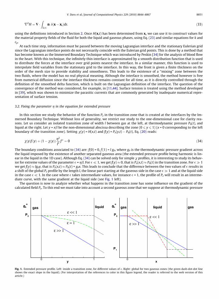
Fig. 1.showsarticle.)


r2H ¼ $ �Z

RðtÞn dðx� xsÞds: ð33Þ

using the definitions introduced in Section 2. Once H(x,t) has been determined from xs we can use it to construct values forthe material property fields of the fluid for both the liquid and gaseous phases, using Eq. (23) and similar equations for k andcp.

At each time step, information must be passed between the moving Lagrangian interface and the stationary Eulerian gridsince the Lagrangian interface points do not necessarily coincide with the Eulerian grid points. This is done by a method thathas become known as the Immersed Boundary Technique which was introduced by Peskin [34] for the analysis of blood flowin the heart. With this technique, the infinitely thin interface is approximated by a smooth distribution function that is usedto distribute the forces at the interface over grid points nearest the interface. In a similar manner, this function is used tointerpolate field variables from the stationary grid to the interface. In this way, the front is given a finite thickness on theorder of the mesh size to provide stability and smoothness. This leads to the existence of a ‘‘mixing” zone between thetwo fluids, where the model has no real physical meaning. Although the interface is smoothed, the method however is freefrom numerical diffusion since the interface thickness remains constant for all time, as it is directly controlled through thedefinition of the smoothed delta function, which is built on the Lagrangian definition of the interface. The question of theconvergence of the method was considered, for example, in [11,44]. Surface tension is treated using the method developedin [39], which was shown to minimize the parasitic currents that are commonly generated by inadequate numerical repre-sentation of surface tension.

3.2. Fixing the parameter g in the equation for extended pressure

In this section we study the behavior of the function Pe in the transition zone that is created at the interfaces by the Im-mersed Boundary Technique. Without loss of generality, we restrict our study to the one-dimensional case for clarity rea-sons. Let us consider an isolated transition zone of width l between gas at the left, at thermodynamic pressure P0(t), andliquid at the right. Let y = x/l be the non-dimensional abscissa describing the zone (0 6 y 6 1) (x = 0 corresponding to the leftboundary of the transition zone). Setting v(y) = H(x,t) and f(y) = Pe(y,t) � P0(t), Eq. (20) reads:

vðyÞf ðyÞ þ ð1� vðyÞÞg2

l2 f 00 ¼ 0 ð34Þ

The boundary conditions associated to (34) are: f(0) = 0, f0(1) = l gP, where gP is the thermodynamic pressure gradient across

the liquid imposed by the existence of another separated gaseous area (the extended pressure profile being harmonic is lin-ear in the liquid in the 1D case). Although Eq. (34) can be solved only for simple v profiles, it is interesting to study its behav-ior for extreme values of the parameter � = g/l. For �� 1, we get f(y) � 0, that is Pe(x,t) � P0(t) in the transition zone. For � 1we get f(y) � lgPy, that is Pe(x,t) � P0(t) + gPx. This leads to conclude that the difference between the two values of � results ina shift of the global Pe profile by the length l, the linear part starting at the gaseous side in the case � 1 and at the liquid sidein the case �� 1. In the case where � takes intermediate values, for instance � = 1, the profile of Pe will result in an interme-diate curve, with the same gradient at the liquid side (see Fig. 1 left).

The question is now to analyze whether what happens in the transition zone has some influence on the gradient of thecalculated field Pe. To this end we must take into account a second gaseous zone that we suppose at thermodynamic pressure

y

P e

0 1

P0

ε = 1

ε >> 1

ε << 1liquidgas

x

P e

0

P0

ε >> 1

ε << 1

liquidgas gas

P1

Extended pressure profile. Left: inside a transition zone, for different values of �. Right: global for two gaseous zones (the green dash-dot-dot linethe exact slope in the liquid). (For interpretation of the references to color in this figure legend, the reader is referred to the web version of this


P1, which will fix the extended pressure gradient inside the liquid. Considering the previous analysis, we can conclude that,in function of the value of �, the linear variation of the calculated Pe takes place between the two gaseous sides (� 1), orbetween the two liquid sides (�� 1). This will change the extended pressure gradient of an amount proportional to thewidth of the transition zone (thus on the order of the mesh size) as is illustrated in Fig. 1(right). The exact value of the gra-dient will be obtained if the linear part of Pe originates at the interface, that is in the middle of the transition zone. Indeed theerror will be reduced with mesh refinement. The error also decreases when the ratio of the transition zone length to liquidwidth is small.

From the previous analysis we can conclude that g should be of the same order than l, although any other value will givethe correct result at grid convergence. In results presented in the following, we fixed g = l = 4dx, dx being the grid cell size.

3.3. Discretization and projection method

The spatial discretization of model (21), (11), (20) is based on centered finite differences for both the convection and dif-fusion terms. A staggered mesh is used, where density, hydrodynamic pressure, extended pressure and temperature arelocated at the center of the cells, while the components of the velocity are located on the faces. We have used here a firstorder explicit temporal discretization, but the extension to semi-implicit second order should be considered in the future.A classical prediction–projection algorithm is used to compute the velocities [15]. The predicted velocity v* is calculatedfrom:

v � vn

dt¼ �vn � rvn þ 1

qnþ1r � sn � 1

qnþ1rpn � 1qnþ1rPn

e þ g ð35Þ

Calculating v* from Eq. (35) needs to calculate first the extended thermodynamic pressure field Pe. To this end Eq. (20) issolved using a BiCGStab solver.

Once v* is known, the projection step consists in extracting vn+1 from v* in such a way that r � vn+1 is zero in the liquid,and equal to its specified value in the gas. This amounts to solving the following Poisson equation for the hydrodynamicpressure:

r � 1qnþ1r/

� �¼ 1

dtðr � v � r � vnþ1Þ ð36Þ

where / = pn+1 � pn is the pressure increment. In the r.h.s. of Eq. (36), r � vn+1 is obtained using the mass conservation Eq.(21a), after the temperature field and 1

Pj

dPj

dt in each gaseous inclusion have been calculated. The latter are calculated using amore convenient form of Eq. (11):

1Pj

dPj

dt¼ 1R

RHjdx

ZR

Hj1T

DTDt

dx�Z

R

Hjr � vdx� �

ð37Þ

The solution of (36) requires a robust matrix solver as the coefficients 1/q are discontinuous, the ratio between the gas andliquid density being generally very large (around 1000 for air–water, much more for example if the liquid is molten glass). Tothis end, we have used a multigrid method that is described in Appendix A.

Once the hydrodynamic pressure is obtained, the velocity is calculated from:

vnþ1 ¼ v � dt1

qnþ1r/ ð38Þ

and the hydrodynamic pressure field is updated by:

pnþ1 ¼ pn þ / ð39Þ

Let us now sum up the complete numerical methodology for the determination of the solution at time t = (n + 1)dt, assumingthe solution known at time t = ndt. Due to the non-linear coupling of the equations, iterations are necessary within each timestep. Indeed, the calculation of 1

PdPdt

� �nþ1j using Eq. (37) makes use of the velocity vn+1 which is unknown at the first iteration. A

convenient first guess for vn+1 can be obtained from the discretization of a simplified momentum equation, where only theexternal forces (extended thermodynamic and gravity forces) are taken into account. It is important to include the extendedpressure force in the first guess in order to avoid selecting the trivial solution consisting of fluid at rest. For this solution, inthe absence of gravity, the hydrodynamic pressure field is obtained as the opposite of the thermodynamic pressure field.

The whole procedure is then:

(1) using the front-tracking method, calculate Hnþ1j in each gaseous zone, Hnþ1 ¼

PNj¼1Hnþ1

j and the new values of k, cp.

(2) Set guessed estimates Pnþ1j ¼ Pn

j ;1P

dPdt

� �nþ1j ¼ 1

PdPdt

� �n

j ; qnþ1 ¼ qn; vnþ1 ¼ vn � dt 1qnrPn

e þ dtg.(3) � �
� solve Eq. (21c) for Tn+1 using 1
PdPdt

nþ1j ;

� calculate the new value of 1P

dPdt

� �nþ1j and Pnþ1

j in each gaseous zone using vn+1, Hn+1 and Tn+1 in (37) and (13);


� calculate qn+1 using (8);� calculate the extended thermodynamic pressure Pnþ1

e ðx; tÞ from (20) using Pnþ1j ; Hnþ1

j ;� calculate r�vn+1 for the Poisson equation using the mass Eq. (21a);� calculate the predicted velocities v* from (35);� solve (36) for the hydrodynamic pressure increment / (multigrid);� project the velocity by (38);� increment the hydrodynamic pressure by (39).

(4) If the computed thermodynamical pressure, density and velocity are different from the ones used at the beginning ofstep 3, restart from step 3 for a new iteration.

In the computations presented in this study, two to four iterations were needed for the convergence of the thermodynam-ical pressure. However the results with or without internal iterations were indistinguishable. This might not be true for othertypes of flows.

For closed gaseous zones, an important point to emphasize is the compatibility relation that must be satisfied when pro-cessing the integration of (37) to calculate 1

PdPdt

� �nþ1in each gaseous zone. In the case where the fluid domain is bounded by

walls and includes N closed gaseous zones, replacing the N Eq. (37) in (21a) and integrating over the whole domain results inthe following relation:

XN

j¼1

ZXjðtÞr � vdx ¼ 0 ð40Þ

However, in the front-tracking method, as already mentioned, there exists a mixing zone, a few cells thick, inside which thevelocity results from the blending of the liquid velocity, which is divergence free, and the gas velocity which is not. Thusthere is no chance that the global balances (40) be zero if the contour of integration for each gaseous zone is located insidethis mixing zone. In fact the contour of integration must include the mixing zone up to the liquid, or equivalently the volumeintegral in (40) must take into account all grid cells for which Hj is not zero. To do this we define an ‘‘enlarged” function Hext

j ,such that:

Hextj ðx; tÞ ¼ 1; if Hjðx; tÞ–0

Hextj ðx; tÞ ¼ 0; if Hjðx; tÞ ¼ 0

(ð41Þ

This enlarged characteristic function is used for the integration of (37) that becomes:

1Pj

dPj

dt¼ 1R

RHjdx

ZR

Hj1T

DTDt

dx�Z

R

Hextj r � vdx

� �ð42Þ

4. Comparison of the 1D low Mach method with a single pressure method on the oscillating water column test case

In this section we highlight the capability of our low Mach method to produce accurate results, even when the time step isof the order of the convective time step, i.e. large compared to an explicit acoustic stability criteria. On the opposite, we showthat a method involving a single pressure (falling in the class of all-Mach methods) needs to be used with small time steps, asit produces very large numerical diffusion when too large time steps are used. It is likely that other single pressure methods,which use more or less the same equation for the pressure, will lead to similar conclusions. This demonstrates that a verysignificant gain in efficiency is obtained using our low Mach method. Moreover the gain is expected to be inversely propor-tional to the Mach number.

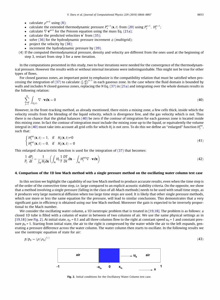
We consider the oscillating water column, a 1D isentropic problem that is treated in [19,18]. The problem is as follows: aclosed 1D tube is filled with a column of water in between of two columns of air. We use the same physical settings as in[19,18] (see Fig. 2). At initial state, xfs = 0.1 and all three columns flow to the right at constant speed u0 = 1 and constant pres-sure p0 = 1. Starting from initial state, the air to the right is compressed by the water while the air to the left expands, gen-erating a pressure difference across the water column. The water column then starts to oscillate. In the following results weuse the isentropic equation of state for air:

p=p0 ¼ ðq=q0Þ1=c ð43Þ

air airu0

10 xfs-xfs-1x

Fig. 2. Initial conditions for the Oscillatory Water Column test case.


with c = 1.4, and initial value q0 = 0.001. This also sets the reference speed of sound value in air ca = (cp0/q0)1/2 = 37.42.Water is considered as incompressible, of constant density qw = 1, and the fluid viscosities are set to zero. In our low Machmodel, the thermodynamic pressure P is used in (43). Let us notice that in this problem the Mach number in the gas neverexceeds 0.03 as we have verified, justifying the low Mach assumption.

In [19], water and air are both treated as compressible fluids, and an explicit method is used. The work in [18] also treatsthe water as compressible, and makes use of a single pressure implicit method aimed at solving all speed multiphase flows,where a Helmholtz equation comparable to the one in [7] is solved for pressure. However in [18] the gas-dynamics equationsare not solved in the gas, avoiding the difficulties of a real two-phase flow computation.

Let us briefly describe the single pressure method that we use for these computations. The flow model is a single pressureisentropic version of (21), that writes:

Fig. 3.boundareader

r � v ¼ �Hðx; tÞ 1q

DqDt ¼ �Hðx; tÞ 1

cpDpDt

@v@t þ v � rv þ 1

qrp ¼ 1qr � sþ g

(ð44Þ

where p is the (unique) pressure that is involved in the equation of state. We first approximate the continuity equation by:

r � vnþ1 ¼ �Hnþ1 1cp

pnþ1 � pn

dtþ vrpnþ1

� �ð45Þ

v* being the predicted velocity and p* obtained by second order backward time extrapolation. This results in the followingequation for the pressure:

r � 1qr/

� �� 1

dt2

Hnþ1

cp/� 1

dtHnþ1

cpvr/ ¼ 1

dtr � v þ 1

dtHnþ1

cpvrpn ð46Þ

with q* = Hn+1q0(p*/p0)c + (1 � Hn+1)qw.We first present the results obtained using our two-pressure low Mach method. For comparison with an explicit method

and the results in [19,18], the time step is calculated as a multiple of the one obtained by using the stability criteria in [19]:

dt ¼ CFLdx

maxjjujj þ cwð47Þ

where cw is the value of speed of sound in water used in [19], cw = 144.94. In the explicit case the stability criterion is CFL 6 1,while a stability criterion based on the convective velocity would allow values of CFL of the order of 100.

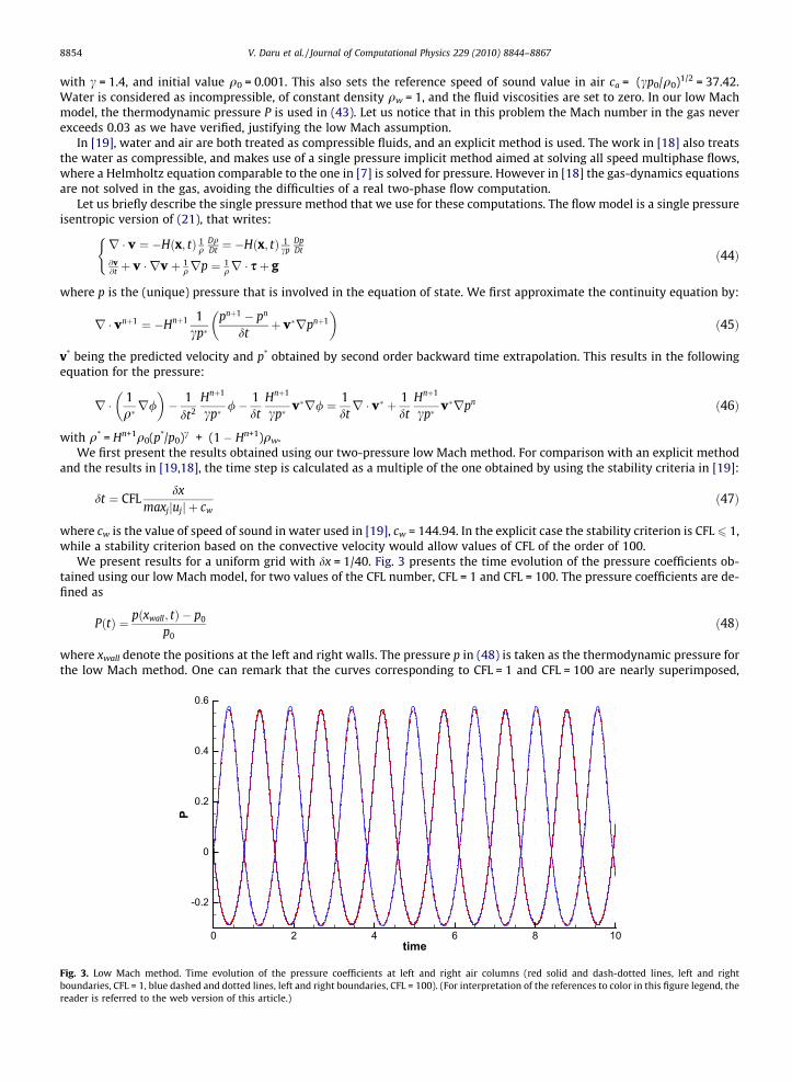
We present results for a uniform grid with dx = 1/40. Fig. 3 presents the time evolution of the pressure coefficients ob-tained using our low Mach model, for two values of the CFL number, CFL = 1 and CFL = 100. The pressure coefficients are de-fined as

PðtÞ ¼ pðxwall; tÞ � p0

p0ð48Þ

where xwall denote the positions at the left and right walls. The pressure p in (48) is taken as the thermodynamic pressure forthe low Mach method. One can remark that the curves corresponding to CFL = 1 and CFL = 100 are nearly superimposed,

time

P

0 2 4 6 8 10

-0.2

0

0.2

0.4

0.6

Low Mach method. Time evolution of the pressure coefficients at left and right air columns (red solid and dash-dotted lines, left and rightries, CFL = 1, blue dashed and dotted lines, left and right boundaries, CFL = 100). (For interpretation of the references to color in this figure legend, theis referred to the web version of this article.)

time

P

0 2 4 6 8 10

-0.2

0

0.2

0.4

0.6

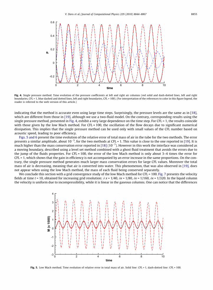
Fig. 4. Single pressure method. Time evolution of the pressure coefficients at left and right air columns (red solid and dash-dotted lines, left and rightboundaries, CFL = 1, blue dashed and dotted lines, left and right boundaries, CFL = 100). (For interpretation of the references to color in this figure legend, thereader is referred to the web version of this article.)


indicating that the method is accurate even using large time steps. Surprisingly, the pressure levels are the same as in [18],which are different from those in [19], although we use a two-fluid model. On the contrary, corresponding results using thesingle pressure method, presented in Fig. 4, exhibit a very large dependence on the time step. For CFL = 1, the results coincidewith those given by the low Mach method. For CFL = 100, the oscillation of the flow decays due to significant numericaldissipation. This implies that the single pressure method can be used only with small values of the CFL number based onacoustic speed, leading to poor efficiency.

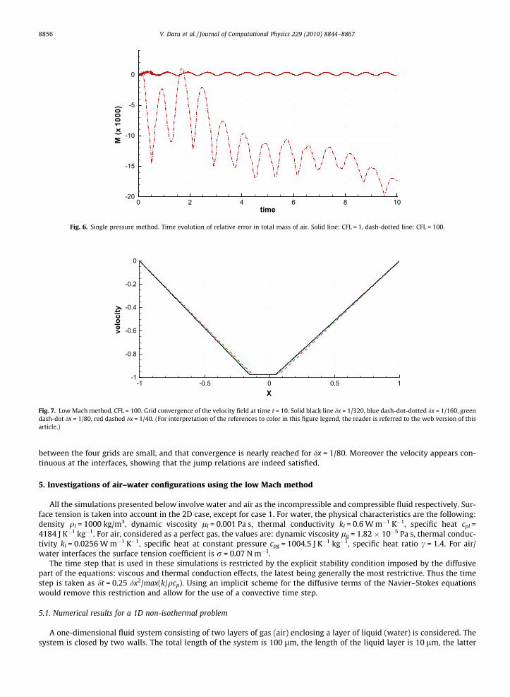
Figs. 5 and 6 present the time evolution of the relative error of total mass of air in the tube for the two methods. The errorpresents a similar amplitude, about 10�3, for the two methods at CFL = 1. This value is close to the one reported in [19]. It ismuch higher than the mass conservation error reported in [18] (10�7). However in this work the interface was considered asa moving boundary, described using a level set method combined with a ghost fluid treatment that avoids the errors due tothe jump of the fluids properties. For CFL = 100, the error of the low Mach method is only about 3–4 times the error forCFL = 1, which shows that the gain in efficiency is not accompanied by an error increase in the same proportions. On the con-trary, the single pressure method generates much larger mass conservation errors for large CFL values. Moreover the totalmass of air is decreasing, meaning that air is converted into water. This phenomenon, that was also observed in [19], doesnot appear when using the low Mach method, the mass of each fluid being conserved separately.

We conclude this section with a grid convergence study of the low Mach method for CFL = 100. Fig. 7 presents the velocityfields at time t = 10, obtained for increasing grid resolution: d x = 1/40, dx = 1/80, dx = 1/160, dx = 1/320. In the liquid columnthe velocity is uniform due to incompressibility, while it is linear in the gaseous columns. One can notice that the differences

time

M(x

1000

)

0 2 4 6 8 10-3

-2

-1

0

1

2

3

4

Fig. 5. Low Mach method. Time evolution of relative error in total mass of air. Solid line: CFL = 1, dash-dotted line: CFL = 100.

time

M(x

1000

)

0 2 4 6 8 10-20

-15

-10

-5

0

Fig. 6. Single pressure method. Time evolution of relative error in total mass of air. Solid line: CFL = 1, dash-dotted line: CFL = 100.

X

velo

city

-1 -0.5 0 0.5 1-1

-0.8

-0.6

-0.4

-0.2

0

Fig. 7. Low Mach method, CFL = 100. Grid convergence of the velocity field at time t = 10. Solid black line dx = 1/320, blue dash-dot-dotted dx = 1/160, greendash-dot dx = 1/80, red dashed dx = 1/40. (For interpretation of the references to color in this figure legend, the reader is referred to the web version of thisarticle.)


between the four grids are small, and that convergence is nearly reached for dx = 1/80. Moreover the velocity appears con-tinuous at the interfaces, showing that the jump relations are indeed satisfied.

5. Investigations of air–water configurations using the low Mach method

All the simulations presented below involve water and air as the incompressible and compressible fluid respectively. Sur-face tension is taken into account in the 2D case, except for case 1. For water, the physical characteristics are the following:density ql = 1000 kg/m3, dynamic viscosity ll = 0.001 Pa s, thermal conductivity kl = 0.6 W m�1 K�1, specific heat cpl =4184 J K�1 kg�1. For air, considered as a perfect gas, the values are: dynamic viscosity lg = 1.82 � 10�5 Pa s, thermal conduc-tivity kl = 0.0256 W m�1 K�1, specific heat at constant pressure cpg = 1004.5 J K�1 kg�1, specific heat ratio c = 1.4. For air/water interfaces the surface tension coefficient is r = 0.07 N m�1.

The time step that is used in these simulations is restricted by the explicit stability condition imposed by the diffusivepart of the equations: viscous and thermal conduction effects, the latest being generally the most restrictive. Thus the timestep is taken as dt = 0.25 dx2/max(k/qcp). Using an implicit scheme for the diffusive terms of the Navier–Stokes equationswould remove this restriction and allow for the use of a convective time step.

5.1. Numerical results for a 1D non-isothermal problem

A one-dimensional fluid system consisting of two layers of gas (air) enclosing a layer of liquid (water) is considered. Thesystem is closed by two walls. The total length of the system is 100 lm, the length of the liquid layer is 10 lm, the latter


being initially situated at the center of the system. The initial thermodynamic conditions are P0 = 101,325 Pa, T0 = 293.15 K.At initial time, the left wall is heated to Tw = 373.15 K, the right wall being insulated. After a transient evolution, a steadystate establishes where the initial positions of the liquid–gas interfaces are recovered, due to mass conservation. In thegas, the density at steady state is unchanged, Tf = Tw everywhere, and Pf = P0�Tf/T0 = 128,976.37 Pa following the perfectgas equation of state. This test case was treated in [10], based on a Arbitrary Lagrangian Eulerian (ALE) method (movingmesh). In this way, the interfaces between liquid and gas are real discontinuities, and there are no errors that could be attrib-uted to the front-tracking method and the existence of a mixing zone. Using an accurate discretization, we can consider theresults given by this code as reference results (see [10] for more details about the ALE procedure).

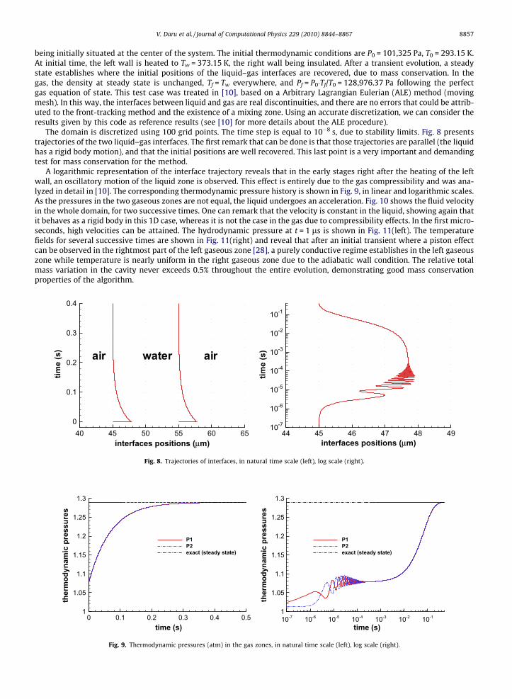
The domain is discretized using 100 grid points. The time step is equal to 10�8 s, due to stability limits. Fig. 8 presentstrajectories of the two liquid–gas interfaces. The first remark that can be done is that those trajectories are parallel (the liquidhas a rigid body motion), and that the initial positions are well recovered. This last point is a very important and demandingtest for mass conservation for the method.

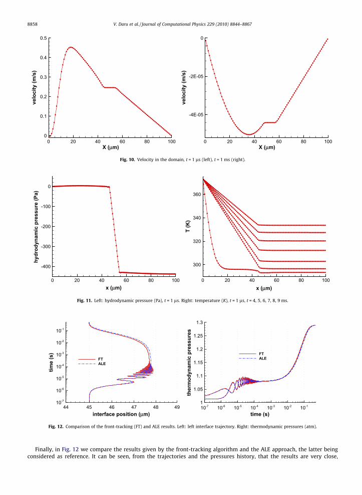
A logarithmic representation of the interface trajectory reveals that in the early stages right after the heating of the leftwall, an oscillatory motion of the liquid zone is observed. This effect is entirely due to the gas compressibility and was ana-lyzed in detail in [10]. The corresponding thermodynamic pressure history is shown in Fig. 9, in linear and logarithmic scales.As the pressures in the two gaseous zones are not equal, the liquid undergoes an acceleration. Fig. 10 shows the fluid velocityin the whole domain, for two successive times. One can remark that the velocity is constant in the liquid, showing again thatit behaves as a rigid body in this 1D case, whereas it is not the case in the gas due to compressibility effects. In the first micro-seconds, high velocities can be attained. The hydrodynamic pressure at t = 1 ls is shown in Fig. 11(left). The temperaturefields for several successive times are shown in Fig. 11(right) and reveal that after an initial transient where a piston effectcan be observed in the rightmost part of the left gaseous zone [28], a purely conductive regime establishes in the left gaseouszone while temperature is nearly uniform in the right gaseous zone due to the adiabatic wall condition. The relative totalmass variation in the cavity never exceeds 0.5% throughout the entire evolution, demonstrating good mass conservationproperties of the algorithm.

interfaces positions (μm)

time

(s)

40 45 50 55 60 650

0.1

0.2

0.3

0.4

waterair air

interfaces positions (μm)

time

(s)

44 45 46 47 48 4910-7

10-6

10-5

10-4

10-3

10-2

10-1

Fig. 8. Trajectories of interfaces, in natural time scale (left), log scale (right).

time (s)

ther

mod

ynam

ic p

ress

ures

0 0.1 0.2 0.3 0.4 0.51

1.05

1.1

1.15

1.2

1.25

1.3

P1P2exact (steady state)

time (s)

ther

mod

ynam

ic p

ress

ures

10-7 10-6 10-5 10-4 10-3 10-2 10-11

1.05

1.1

1.15

1.2

1.25

1.3

P1P2exact (steady state)

Fig. 9. Thermodynamic pressures (atm) in the gas zones, in natural time scale (left), log scale (right).

X (μm)

velo

city

(m/s

)

0 20 40 60 80 1000

0.1

0.2

0.3

0.4

0.5

X (μm)

velo

city

(m/s

)

0 20 40 60 80 100

-4E-05

-2E-05

0

Fig. 10. Velocity in the domain, t = 1 ls (left), t = 1 ms (right).

x (μm) x (μm)

hydr

odyn

amic

pre

ssur

e (P

a)

0 20 40 60 80 100

-400

-300

-200

-100

0T

(K)

0 20 40 60 80 100

300

320

340

360

Fig. 11. Left: hydrodynamic pressure (Pa), t = 1 ls. Right: temperature (K), t = 1 ls, t = 4, 5, 6, 7, 8, 9 ms.

interface position (μm)

time

(s)

44 45 46 47 48 4910-7

10-6

10-5

10-4

10-3

10-2

10-1

FTALE

time (s)

ther

mod

ynam

ic p

ress

ures

10-7 10-6 10-5 10-4 10-3 10-2 10-11

1.05

1.1

1.15

1.2

1.25

1.3

FTALE

Fig. 12. Comparison of the front-tracking (FT) and ALE results. Left: left interface trajectory. Right: thermodynamic pressures (atm).


Finally, in Fig. 12 we compare the results given by the front-tracking algorithm and the ALE approach, the latter beingconsidered as reference. It can be seen, from the trajectories and the pressures history, that the results are very close,


although the front-tracking algorithm is only first order in time. This validates the low Mach compressible/incompressibleapproach in the front-tracking framework.

5.2. 2D numerical results

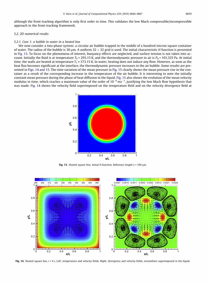
5.2.1. Case 1: a bubble in water in a heated boxWe now consider a two-phase system: a circular air bubble trapped in the middle of a hundred micron square container

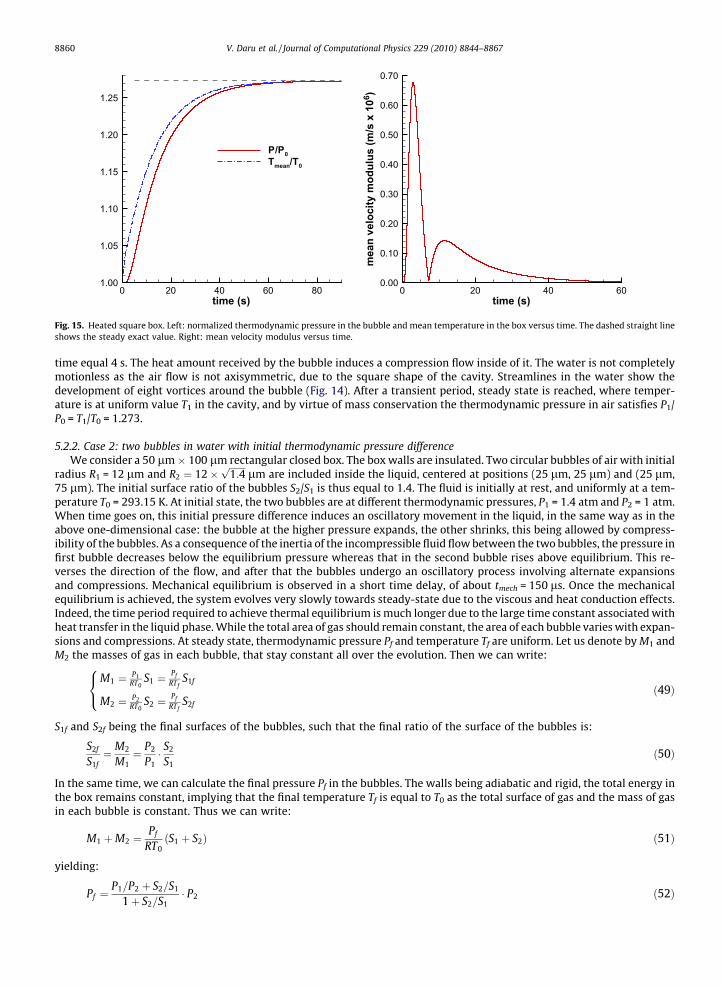
of water. The radius of the bubble is 30 lm. A uniform 32 � 32 grid is used. The initial characteristic H function is presentedin Fig. 13. To focus on the phenomena of interest, buoyancy effects are neglected, and surface tension is not taken into ac-count. Initially the fluid is at temperature T0 = 293.15 K, and the thermodynamic pressure in air is P0 = 101,325 Pa. At initialtime, the walls are heated at temperature T1 = 373.15 K. In water, heating does not induce any flow. However, as soon as theheat flux becomes significant at the interface, the thermodynamic pressure increases in the air bubble. Some results are pre-sented in Figs. 14 and 15. The time variation of the mean pressure in Fig. 15 clearly shows the mean pressure rise in the con-tainer as a result of the corresponding increase in the temperature of the air bubble. It is interesting to note the initiallyconstant mean pressure during the phase of heat diffusion in the liquid. Fig. 15 also shows the evolution of the mean velocitymodulus in time, which reaches a maximum value of the order of 10�6 ms�1, justifying the low Mach flow hypothesis thatwas made. Fig. 14 shows the velocity field superimposed on the temperature field and on the velocity divergence field at

Fig. 13. Heated square box. Initial H function. Reference length L = 100 lm.

x/L

y/L

0 0.2 0.4 0.6 0.8 10

0.2

0.4

0.6

0.8

1296 304 312 320 328 336 344 352 360 368

x/L

y/L

0 0.2 0.4 0.6 0.8 10

0.2

0.4

0.6

0.8

1-0.0027 -0.0019 -0.0011 -0.0003 0.0005 0.0013 0.0021 0.0029

Fig. 14. Heated square box, t = 4 s. Left: temperature and velocity fields. Right: divergence and velocity fields, streamlines superimposed in the liquid.

time (s)0 20 40 60 80

1.00

1.05

1.10

1.15

1.20

1.25

P/P0Tmean/T0

time (s)

mea

n ve

loci

ty m

odul

us (m

/s x

106 )

0 20 40 600.00

0.10

0.20

0.30

0.40

0.50

0.60

0.70

Fig. 15. Heated square box. Left: normalized thermodynamic pressure in the bubble and mean temperature in the box versus time. The dashed straight lineshows the steady exact value. Right: mean velocity modulus versus time.


time equal 4 s. The heat amount received by the bubble induces a compression flow inside of it. The water is not completelymotionless as the air flow is not axisymmetric, due to the square shape of the cavity. Streamlines in the water show thedevelopment of eight vortices around the bubble (Fig. 14). After a transient period, steady state is reached, where temper-ature is at uniform value T1 in the cavity, and by virtue of mass conservation the thermodynamic pressure in air satisfies P1/P0 = T1/T0 = 1.273.

5.2.2. Case 2: two bubbles in water with initial thermodynamic pressure differenceWe consider a 50 lm � 100 lm rectangular closed box. The box walls are insulated. Two circular bubbles of air with initial

radius R1 = 12 lm and R2 ¼ 12�ffiffiffiffiffiffiffi1:4p

lm are included inside the liquid, centered at positions (25 lm, 25 lm) and (25 lm,75 lm). The initial surface ratio of the bubbles S2/S1 is thus equal to 1.4. The fluid is initially at rest, and uniformly at a tem-perature T0 = 293.15 K. At initial state, the two bubbles are at different thermodynamic pressures, P1 = 1.4 atm and P2 = 1 atm.When time goes on, this initial pressure difference induces an oscillatory movement in the liquid, in the same way as in theabove one-dimensional case: the bubble at the higher pressure expands, the other shrinks, this being allowed by compress-ibility of the bubbles. As a consequence of the inertia of the incompressible fluid flow between the two bubbles, the pressure infirst bubble decreases below the equilibrium pressure whereas that in the second bubble rises above equilibrium. This re-verses the direction of the flow, and after that the bubbles undergo an oscillatory process involving alternate expansionsand compressions. Mechanical equilibrium is observed in a short time delay, of about tmech = 150 ls. Once the mechanicalequilibrium is achieved, the system evolves very slowly towards steady-state due to the viscous and heat conduction effects.Indeed, the time period required to achieve thermal equilibrium is much longer due to the large time constant associated withheat transfer in the liquid phase. While the total area of gas should remain constant, the area of each bubble varies with expan-sions and compressions. At steady state, thermodynamic pressure Pf and temperature Tf are uniform. Let us denote by M1 andM2 the masses of gas in each bubble, that stay constant all over the evolution. Then we can write:

M1 ¼ P1RT0

S1 ¼Pf

RTfS1f

M2 ¼ P2RT0

S2 ¼Pf

RTfS2f

8<: ð49Þ

S1f and S2f being the final surfaces of the bubbles, such that the final ratio of the surface of the bubbles is:

S2f

S1f¼ M2

M1¼ P2

P1� S2

S1ð50Þ

In the same time, we can calculate the final pressure Pf in the bubbles. The walls being adiabatic and rigid, the total energy inthe box remains constant, implying that the final temperature Tf is equal to T0 as the total surface of gas and the mass of gasin each bubble is constant. Thus we can write:

M1 þM2 ¼Pf

RT0ðS1 þ S2Þ ð51Þ

yielding:

Pf ¼P1=P2 þ S2=S1

1þ S2=S1� P2 ð52Þ

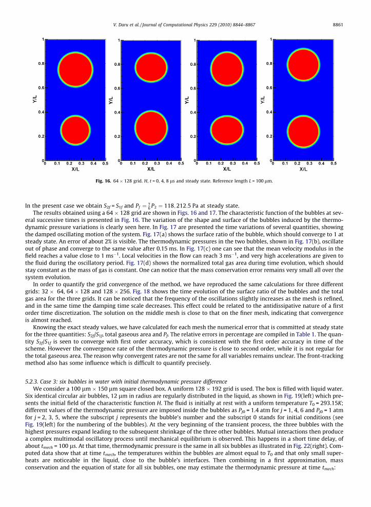
Fig. 16. 64 � 128 grid. H, t = 0, 4, 8 ls and steady state. Reference length L = 100 lm.


In the present case we obtain S2f = S1f and Pf ¼ 76 P2 ¼ 118;212:5 Pa at steady state.

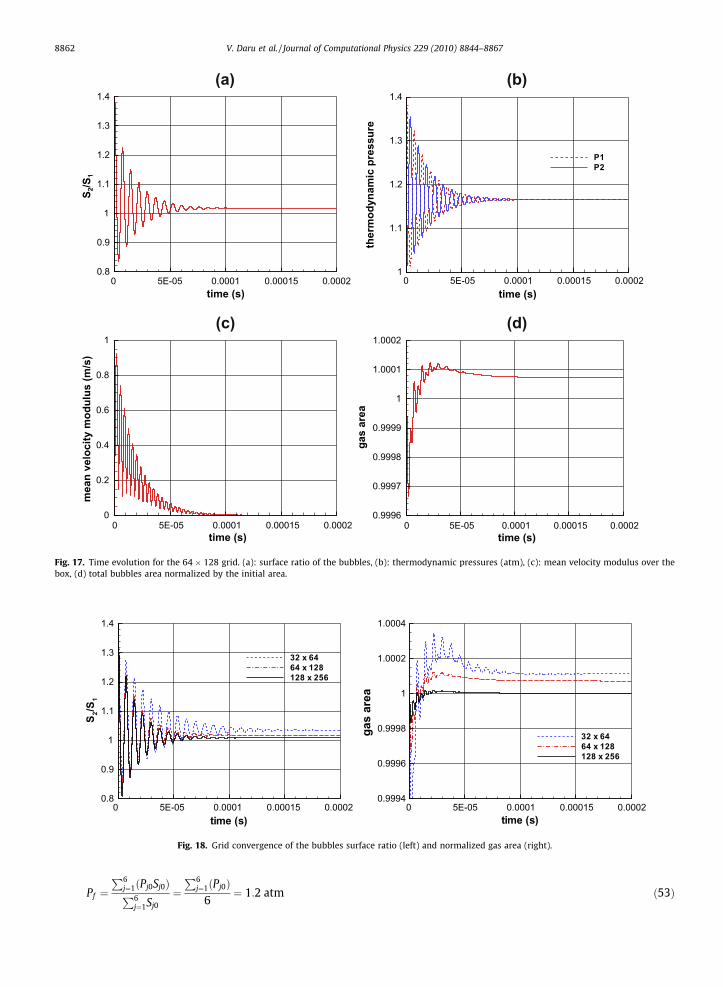
The results obtained using a 64 � 128 grid are shown in Figs. 16 and 17. The characteristic function of the bubbles at sev-eral successive times is presented in Fig. 16. The variation of the shape and surface of the bubbles induced by the thermo-dynamic pressure variations is clearly seen here. In Fig. 17 are presented the time variations of several quantities, showingthe damped oscillating motion of the system. Fig. 17(a) shows the surface ratio of the bubble, which should converge to 1 atsteady state. An error of about 2% is visible. The thermodynamic pressures in the two bubbles, shown in Fig. 17(b), oscillateout of phase and converge to the same value after 0.15 ms. In Fig. 17(c) one can see that the mean velocity modulus in thefield reaches a value close to 1 ms�1. Local velocities in the flow can reach 3 ms�1, and very high accelerations are given tothe fluid during the oscillatory period. Fig. 17(d) shows the normalized total gas area during time evolution, which shouldstay constant as the mass of gas is constant. One can notice that the mass conservation error remains very small all over thesystem evolution.

In order to quantify the grid convergence of the method, we have reproduced the same calculations for three differentgrids: 32 � 64, 64 � 128 and 128 � 256. Fig. 18 shows the time evolution of the surface ratio of the bubbles and the totalgas area for the three grids. It can be noticed that the frequency of the oscillations slightly increases as the mesh is refined,and in the same time the damping time scale decreases. This effect could be related to the antidissipative nature of a firstorder time discretization. The solution on the middle mesh is close to that on the finer mesh, indicating that convergenceis almost reached.

Knowing the exact steady values, we have calculated for each mesh the numerical error that is committed at steady statefor the three quantities: S2f/S1f, total gaseous area and Pf. The relative errors in percentage are compiled in Table 1. The quan-tity S2f/S1f is seen to converge with first order accuracy, which is consistent with the first order accuracy in time of thescheme. However the convergence rate of the thermodynamic pressure is close to second order, while it is not regular forthe total gaseous area. The reason why convergent rates are not the same for all variables remains unclear. The front-trackingmethod also has some influence which is difficult to quantify precisely.

5.2.3. Case 3: six bubbles in water with initial thermodynamic pressure differenceWe consider a 100 lm � 150 lm square closed box. A uniform 128 � 192 grid is used. The box is filled with liquid water.

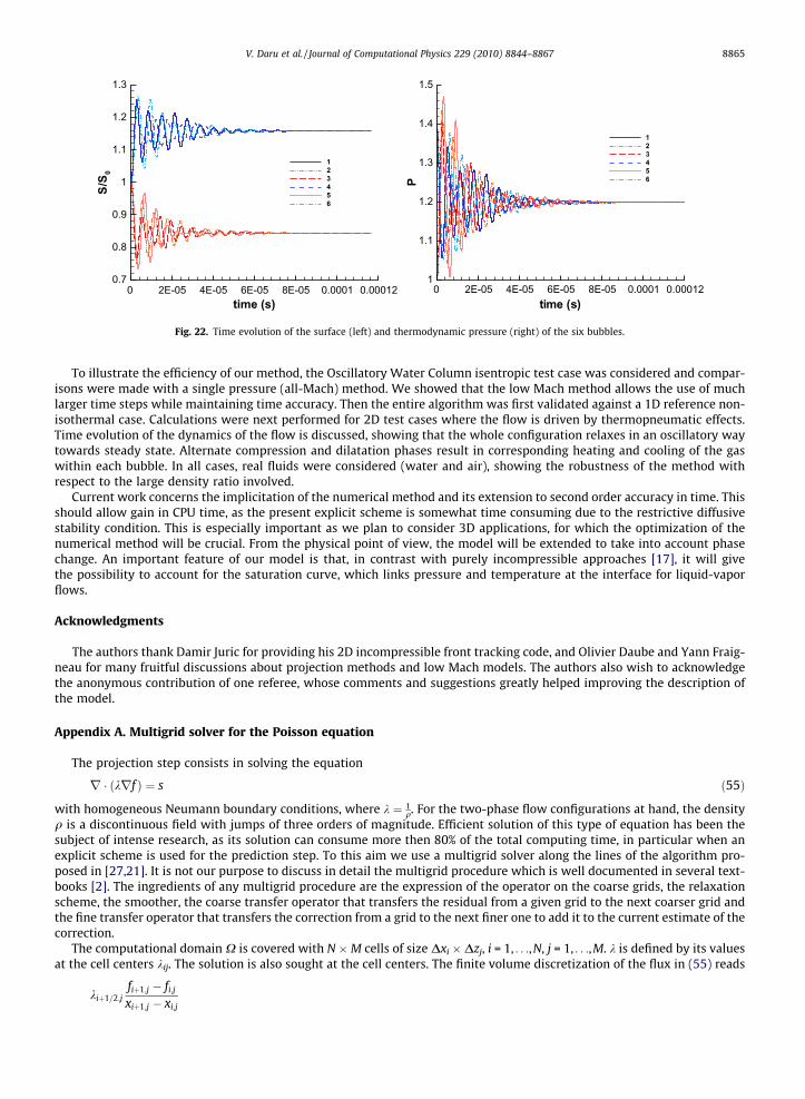
Six identical circular air bubbles, 12 lm in radius are regularly distributed in the liquid, as shown in Fig. 19(left) which pre-sents the initial field of the characteristic function H. The fluid is initially at rest with a uniform temperature T0 = 293.15K;different values of the thermodynamic pressure are imposed inside the bubbles as Pj0 = 1.4 atm for j = 1, 4, 6 and Pj0 = 1 atmfor j = 2, 3, 5, where the subscript j represents the bubble’s number and the subscript 0 stands for initial conditions (seeFig. 19(left) for the numbering of the bubbles). At the very beginning of the transient process, the three bubbles with thehighest pressures expand leading to the subsequent shrinkage of the three other bubbles. Mutual interactions then producea complex multimodal oscillatory process until mechanical equilibrium is observed. This happens in a short time delay, ofabout tmech = 100 ls. At that time, thermodynamic pressure is the same in all six bubbles as illustrated in Fig. 22(right). Com-puted data show that at time tmech, the temperatures within the bubbles are almost equal to T0 and that only small super-heats are noticeable in the liquid, close to the bubble’s interfaces. Then combining in a first approximation, massconservation and the equation of state for all six bubbles, one may estimate the thermodynamic pressure at time tmech:

(b)(a)

time (s)

S 2/S

1

0 5E-05 0.0001 0.00015 0.00020.8

0.9

1

1.1

1.2

1.3

1.4

time (s)

ther

mod

ynam

ic p

ress

ure

0 5E-05 0.0001 0.00015 0.00021

1.1

1.2

1.3

1.4

P1P2

(d)(c)

time (s)

mea

n ve

loci

ty m

odul

us (m

/s)

0 5E-05 0.0001 0.00015 0.00020

0.2

0.4

0.6

0.8

1

time (s)

gas

area

0 5E-05 0.0001 0.00015 0.00020.9996

0.9997

0.9998

0.9999

1

1.0001

1.0002

Fig. 17. Time evolution for the 64 � 128 grid. (a): surface ratio of the bubbles, (b): thermodynamic pressures (atm), (c): mean velocity modulus over thebox, (d) total bubbles area normalized by the initial area.

time (s)

S 2/S1

0 5E-05 0.0001 0.00015 0.00020.8

0.9

1

1.1

1.2

1.3

1.4

32 x 6464 x 128128 x 256

time (s)

gas

area

0 5E-05 0.0001 0.00015 0.00020.9994

0.9996

0.9998

1

1.0002

1.0004

32 x 6464 x 128128 x 256

Fig. 18. Grid convergence of the bubbles surface ratio (left) and normalized gas area (right).


Pf ¼P6

j¼1ðPj0Sj0ÞP6j¼1Sj0

¼P6

j¼1ðPj0Þ6

¼ 1:2 atm ð53Þ

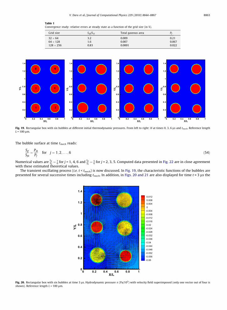
Table 1Convergence study: relative errors at steady state as a function of the grid size (in %).

Grid size S2f/S1f Total gaseous area Pf

32 � 64 3.2 0.009 0.2164 � 128 1.6 0.007 0.067128 � 256 0.83 0.0001 0.022

Fig. 19. Rectangular box with six bubbles at different initial thermodynamic pressures. From left to right: H at times 0, 3, 6 ls and tmech. Reference lengthL = 100 lm.


The bubble surface at time tmech reads:

Fig. 20.shown)

Sjf

Sj0¼ Pj0

Pffor j ¼ 1;2; . . . ;6 ð54Þ

Numerical values are Sjf

S0¼ 7

6 for j = 1, 4, 6 and Sjf

S0¼ 5

6 for j = 2, 3, 5. Computed data presented in Fig. 22 are in close agreementwith these estimated theoretical values.

The transient oscillating process (i.e. t < tmech) is now discussed. In Fig. 19, the characteristic functions of the bubbles arepresented for several successive times including tmech. In addition, in Figs. 20 and 21 are also displayed for time t = 3 ls the

X/L

Y/L

0 0.2 0.4 0.6 0.8 10

0.2

0.4

0.6

0.8

1

1.2

1.4

0.0120.0080.0040-0.004-0.008-0.012-0.016-0.02-0.024-0.028-0.032-0.036-0.04-0.044-0.048-0.052-0.056-0.06

Rectangular box with six bubbles at time 3 ls. Hydrodynamic pressure p (Pa/105) with velocity field superimposed (only one vector out of four is. Reference length L = 100 lm.

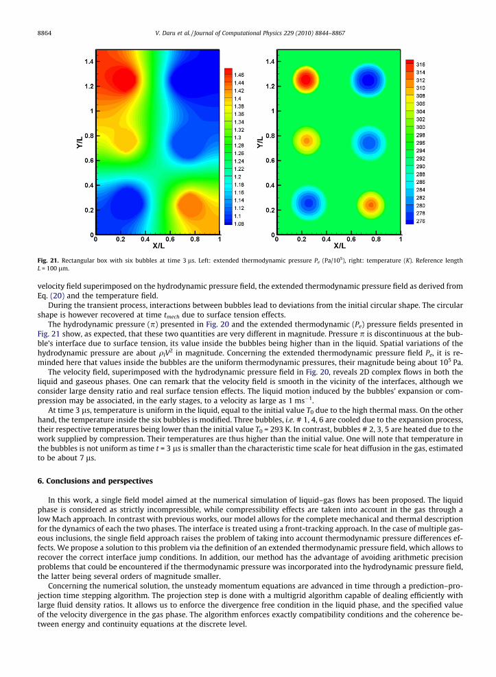
Fig. 21. Rectangular box with six bubbles at time 3 ls. Left: extended thermodynamic pressure Pe (Pa/105), right: temperature (K). Reference lengthL = 100 lm.


velocity field superimposed on the hydrodynamic pressure field, the extended thermodynamic pressure field as derived fromEq. (20) and the temperature field.

During the transient process, interactions between bubbles lead to deviations from the initial circular shape. The circularshape is however recovered at time tmech due to surface tension effects.

The hydrodynamic pressure (p) presented in Fig. 20 and the extended thermodynamic (Pe) pressure fields presented inFig. 21 show, as expected, that these two quantities are very different in magnitude. Pressure p is discontinuous at the bub-ble’s interface due to surface tension, its value inside the bubbles being higher than in the liquid. Spatial variations of thehydrodynamic pressure are about qlV

2 in magnitude. Concerning the extended thermodynamic pressure field Pe, it is re-minded here that values inside the bubbles are the uniform thermodynamic pressures, their magnitude being about 105 Pa.

The velocity field, superimposed with the hydrodynamic pressure field in Fig. 20, reveals 2D complex flows in both theliquid and gaseous phases. One can remark that the velocity field is smooth in the vicinity of the interfaces, although weconsider large density ratio and real surface tension effects. The liquid motion induced by the bubbles’ expansion or com-pression may be associated, in the early stages, to a velocity as large as 1 ms�1.

At time 3 ls, temperature is uniform in the liquid, equal to the initial value T0 due to the high thermal mass. On the otherhand, the temperature inside the six bubbles is modified. Three bubbles, i.e. # 1, 4, 6 are cooled due to the expansion process,their respective temperatures being lower than the initial value T0 = 293 K. In contrast, bubbles # 2, 3, 5 are heated due to thework supplied by compression. Their temperatures are thus higher than the initial value. One will note that temperature inthe bubbles is not uniform as time t = 3 ls is smaller than the characteristic time scale for heat diffusion in the gas, estimatedto be about 7 ls.

6. Conclusions and perspectives

In this work, a single field model aimed at the numerical simulation of liquid–gas flows has been proposed. The liquidphase is considered as strictly incompressible, while compressibility effects are taken into account in the gas through alow Mach approach. In contrast with previous works, our model allows for the complete mechanical and thermal descriptionfor the dynamics of each the two phases. The interface is treated using a front-tracking approach. In the case of multiple gas-eous inclusions, the single field approach raises the problem of taking into account thermodynamic pressure differences ef-fects. We propose a solution to this problem via the definition of an extended thermodynamic pressure field, which allows torecover the correct interface jump conditions. In addition, our method has the advantage of avoiding arithmetic precisionproblems that could be encountered if the thermodynamic pressure was incorporated into the hydrodynamic pressure field,the latter being several orders of magnitude smaller.

Concerning the numerical solution, the unsteady momentum equations are advanced in time through a prediction–pro-jection time stepping algorithm. The projection step is done with a multigrid algorithm capable of dealing efficiently withlarge fluid density ratios. It allows us to enforce the divergence free condition in the liquid phase, and the specified valueof the velocity divergence in the gas phase. The algorithm enforces exactly compatibility conditions and the coherence be-tween energy and continuity equations at the discrete level.

time (s)

S/S 0

0 2E-05 4E-05 6E-05 8E-05 0.0001 0.000120.7

0.8

0.9

1

1.1

1.2

1.3

123456

time (s)

P

0 2E-05 4E-05 6E-05 8E-05 0.0001 0.000121

1.1

1.2

1.3

1.4

1.5

123456

Fig. 22. Time evolution of the surface (left) and thermodynamic pressure (right) of the six bubbles.


To illustrate the efficiency of our method, the Oscillatory Water Column isentropic test case was considered and compar-isons were made with a single pressure (all-Mach) method. We showed that the low Mach method allows the use of muchlarger time steps while maintaining time accuracy. Then the entire algorithm was first validated against a 1D reference non-isothermal case. Calculations were next performed for 2D test cases where the flow is driven by thermopneumatic effects.Time evolution of the dynamics of the flow is discussed, showing that the whole configuration relaxes in an oscillatory waytowards steady state. Alternate compression and dilatation phases result in corresponding heating and cooling of the gaswithin each bubble. In all cases, real fluids were considered (water and air), showing the robustness of the method withrespect to the large density ratio involved.

Current work concerns the implicitation of the numerical method and its extension to second order accuracy in time. Thisshould allow gain in CPU time, as the present explicit scheme is somewhat time consuming due to the restrictive diffusivestability condition. This is especially important as we plan to consider 3D applications, for which the optimization of thenumerical method will be crucial. From the physical point of view, the model will be extended to take into account phasechange. An important feature of our model is that, in contrast with purely incompressible approaches [17], it will givethe possibility to account for the saturation curve, which links pressure and temperature at the interface for liquid-vaporflows.

Acknowledgments

The authors thank Damir Juric for providing his 2D incompressible front tracking code, and Olivier Daube and Yann Fraig-neau for many fruitful discussions about projection methods and low Mach models. The authors also wish to acknowledgethe anonymous contribution of one referee, whose comments and suggestions greatly helped improving the description ofthe model.

Appendix A. Multigrid solver for the Poisson equation

The projection step consists in solving the equation

r � ðkrf Þ ¼ s ð55Þ

with homogeneous Neumann boundary conditions, where k ¼ 1q. For the two-phase flow configurations at hand, the density

q is a discontinuous field with jumps of three orders of magnitude. Efficient solution of this type of equation has been thesubject of intense research, as its solution can consume more then 80% of the total computing time, in particular when anexplicit scheme is used for the prediction step. To this aim we use a multigrid solver along the lines of the algorithm pro-posed in [27,21]. It is not our purpose to discuss in detail the multigrid procedure which is well documented in several text-books [2]. The ingredients of any multigrid procedure are the expression of the operator on the coarse grids, the relaxationscheme, the smoother, the coarse transfer operator that transfers the residual from a given grid to the next coarser grid andthe fine transfer operator that transfers the correction from a grid to the next finer one to add it to the current estimate of thecorrection.

The computational domain X is covered with N �M cells of size Dxi � Dzj, i = 1, . . .,N, j = 1, . . .,M. k is defined by its valuesat the cell centers kij. The solution is also sought at the cell centers. The finite volume discretization of the flux in (55) reads

kiþ1=2;jfiþ1;j � fi;j

xiþ1;j � xi;j


at the east side of the cell with similar expressions for the other faces. Following [27,21], the main idea of the algorithm is toenforce continuity of fluxes at the cell interfaces. It is well known that this is achieved by defining ki+1/2,j as the harmonicaverage of ki+1,j and ki,j that is

2kiþ1=2;j

¼ 1kiþ1;j

þ 1ki;j

The coarse grids are defined by merging together two cells in each direction, which sets the cell boundaries as guidelines todefine the coarse grids. The cell centers are defined accordingly. Once the grid is defined, we define kij on a grid from theweighted average of the four corresponding values on the next finer grid. Likewise, the residual restriction transfer operatoris defined as the sum of the residuals of the 4 corresponding cells, which ensures conservativity of the mass unbalance.

The relaxation scheme is a simple SOR iteration whose acceleration parameter is adjusted empirically in order to producethe best convergence rate.

Concerning the interpolation operator for the correction of the error, it is also defined to ensure a constant flux interpo-lation in the following way: for each coarse cell, 8 constant flux interpolations are first produced from coarse cell neighbors, 4at the middle of the faces, 4 at the corners. With straightforward notations,

fe ¼kiþ1;jfiþ1;j þ ki;jfi;j

kiþ1;j þ ki;j; f en ¼

kiþ1;jþ1fiþ1;jþ1 þ ki;jfi;j

kiþ1;jþ1 þ ki;j

with similar expressions for the other values. For each coarse cell, the corresponding 4 fine cell values are then defined as thearithmetic mean of the interpolated coarse values at the four corresponding corners.

In addition, for other application purposes, we define a solid phase indicator allowing for the presence of solid parts. Onehas then to solve the pressure equation with the homogeneous Neumann boundary conditions imposed at the fluid solidinterface. The difficulty is to take into account this boundary condition to construct the operator in a systematic way. Todo this, we recursively define the solid indicator of the coarse grids with the following principle: a coarse grid is consideredas liquid iff one of the four corresponding fine cells is liquid. With all the ingredients, all operators can be recursively definedon all grids, allowing for an automatic algorithm once the various indicator functions are defined on the finest grid.

References

[1] T. Bonometti, J. Magnaudet, An interface-capturing method for incompressible two-phase flows. Validation and application to bubble dynamics, Int. J.Multiphase Flows 33 (2007) 109–133.

[2] W.L. Briggs, V.E. Henson, S.F. McCormick, A Multigrid Tutorial, second ed., SIAM, 2000.[3] A. Caboussat, A numerical method for the simulation of free surface flows with surface tension, Comput. Fluids 35 (2006) 1205–1216.[4] A. Caboussat, M. Picasso, J. Rappaz, Numerical simulation of free surface incompressible liquid flows surrounded by compressible gas, J. Comput. Phys.

203 (2005) 626–649.[5] R. Caiden, R.P. Fedkiw, C. Anderson, A numerical method for two-phase flow consisting of separate compressible and incompressible regions, J. Comput.

Phys. 166 (2001) 1–27.[6] D. Chenoweth, S. Paolucci, Natural convection in an enclosed vertical air layer with large horizontal temperature differences, J. Fluid Mech. 169 (1986)

173–210.[7] V. Daru, M.C. Duluc, O. Le Maı̂tre, D. Juric, P. Le Quéré, Modélisation et simulation numérique du changement de phase liquide-vapeur en cavité, CRAS

Mécanique 224 (2006) 25–33.[8] J.M. Delhaye, Jump conditions and entropy sources in two-phase systems. Local instant formulation, Int. J. Multiphase Flow 1 (1974) 395–409.[9] S. Dellacherie, Numerical resolution of a potential diphasic low Mach number system, J. Comput. Phys. 223 (2007) 151–187.

[10] M.C. Duluc, O. Le Maı̂tre, V. Daru, P. Le Quéré, Numerical study of liquid inclusion oscillations inside a closed 1-D microchannel filled with gas,Microfluidics Nanofluidics 6 (2009) 163–177.

[11] A. Esmaeeli, G. Tryggvason, Direct numerical simulations of bubbly flows. Part 1. Low Reynolds number arrays, J. Fluid Mech. 377 (1998) 313–345.[12] A. Esmaeeli, G. Tryggvason, Computations of film boiling. Part I: numerical method, Int. J. Heat Mass Transfer 47 (2004) 5451–5461.[13] C. Forester, A. Emery, A computational method for low Mach number unsteady compressible free convective flows, J. Comput. Phys. 10 (3) (1972) 487–

502.[14] X. Geng, H. Yuan, N. O~guz, A. Prosperetti, The oscillation of gas bubbles in tubes: experimental results, J. Acoust. Soc. Am. 106 (2) (1999) 674–681.[15] K. Goda, A multistep technique with implicit difference schemes for calculating two- or three-dimensional cavity flows, J. Comput. Phys. 30 (1) (1979)

76–95.[16] M. Ida, An improved unified solver for compressible and incompressible fluids involving free surfaces. II. Multi-time-step integration and applications,

Comput. Phys. Comm. 150 (3) (2003) 300–322.[17] D. Juric, G. Tryggvason, Computations of boiling flows, Int. J. Multiphase Flow 24 (3) (1998) 387–410.[18] S.Y. Kadioglu, M. Sussman, S. Osher, et al, A second order primitive preconditioner for solving all speed multi-phase flows, J. Comput. Phys. 209 (2)

(2005) 477–503.[19] B. Koren, M.R. Lewis, E.H. van Brummelen, B. van Leer, Riemann-problem and level-set approaches for homentropic two-fluid flow computations, J.

Comput. Phys. 181 (11) (2002) 654–674.[20] P. Kuszla, V. Daru, Multifluid computation of droplets impact, Lecture Notes in Physics, vol. 515, C.H. Bruneau ed., Springer, 1998, pp. 524–529.[21] D. Kwak, J. Lee, Multigrid algorithm for the cell-centered finite difference method II: discontinuous coefficient case, Numer. Methods Partial

Differential Equations 20 (5) (2004) 742–764.[22] N. Kwatra, J. Su, J.T. Gretarsson, R. Fedkiw, A method for avoiding the acoustic time step restriction in compressible flow, J. Comput. Phys. 228 (11)

(2009) 4146–4161.[23] B. Lafaurie, C. Nardone, R. Scardovelli, S. Zaleski, G. Zanetti, Modelling merging and fragmentation in multiphase flows with surfer, J. Comput. Phys. 113

(1994) 134–147.[24] P. Le Quéré, R. Masson, P. Perrot, A Chebyshev collocation algorithm for 2D non-Boussinesq convection, J. Comput. Phys. 103 (2) (1992) 320–335.[25] P. Le Quéré, C. Weisman, H. Paillère, J. Vierendeels, E. Dick, R. Becker, M. Braack, J. Locke, Modelling of natural convection flows with large temperature

differences. Part 1: reference solutions, Math. Model. Numer. Anal. 39 (3) (2005) 609–616.


[26] D. Legendre, J. Borée, J. Magnaudet, Thermal and dynamic evolution of a spherical bubble moving steadily in a superheated or subcooled liquid, Phys.Fluids 10 (1998) 1256–1272.

[27] C. Liu, Z. Liu, S. McCormick, An efficient multigrid scheme for elliptic equations with discontinuous coefficients, Comm. Appl. Numer. Methods 8 (1992)621–631.

[28] Y. Masuda, T. Aizawa, M. Kanakubo, N. Saito, Y. Ikushima, Numerical simulation of two-dimensional piston effect and natural convection in a squarecavity heated from one side, Int. Comm. Heat Mass Transfer 31 (2) (2004) 151–160.

[29] T. Ménard, S. Tanguy, A. Berlemont, Coupling level set/vof/ghost fluid methods: validation and application to 3D simulation of the primary break-up ofa liquid jet, Int. J. Multiphase Flow 33 (2007) 510–524.

[30] N. O~guz, A. Prosperetti, The natural frequency of oscillation of gas bubbles in tubes, J. Acoust. Soc. Am. 103 (6) (1998) 3301–3308.[31] E. Ory, H. Yuan, A. Prosperetti, S. Popinet, S. Zaleski, Growth and collapse of a vapour bubble in a narrow tube, Phys. Fluids 12 (6) (2000) 1268–1277.[32] H. Paillère, P. Le Quéré, C. Weisman, J. Vierendeels, E. Dick, Modelling of natural convection flows with large temperature differences. Part 2:

contributions, Math. Model. Numer. Anal. 39 (3) (2005) 617–621.[33] S. Paolucci, Sandia National Lab., Report SAND 82-8257, 1982 (unpublished).[34] C.S. Peskin, Numerical analysis of blood flow in the heart, J. Comput. Phys. 25 (1977) 220–252.[35] A. Prosperetti, G. Tryggvason, Computational Methods for Multiphase Flows, Cambridge University Press, 2007.[36] R. Saurel, R. Abgrall, A multiphase Godunov method for compressible multifluid and multiphase flows, J. Comput. Phys. 150 (1999) 425–467.[37] R. Scardovelli, S. Zaleski, Direct numerical simulation of free surface and interfacial flow, Ann. Rev. Fluid Mech. 31 (1999) 567–603.[38] J. Sethian, Level Set Methods and Fast Marching Methods, Cambridge University Press, 1999.[39] S. Shin, S. Abdel-Khalik, V. Daru, D. Juric, Accurate representation of surface tension using the level contour reconstruction method, J. Comput. Phys.

203 (2) (2005) 493–516.[40] S. Shin, D. Juric, Modeling three-dimensional multiphase flow using a level contour reconstruction method for front-tracking without connectivity, J.

Comput. Phys. 180 (2002) 427–470.[41] K.M. Shyue, An efficient shock-capturing algorithm for compressible multicomponent problems, J. Comput. Phys. 142 (1998) 208–242.[42] M. Sussman, P. Smereka, S. Osher, A level set approach for computing solutions in incompressible two-phase flows, J. Comput. Phys. 114 (1994) 146–

159.[43] S. Tanguy, A. Berlemont, Application of a level set method for simulation of droplet collisions, Int. J. Multiphase Flow 31 (2005) 1015–1035.[44] G. Tryggvason, B. Bunner, A. Esmaeeli, D. Juric, N. Al-Rawahi, W. Tauber, J. Han, S. Nas, Y. Jan, A front-tracking method for the computations of

multiphase flow, J. Comput. Phys. 169 (2) (2001) 708–759.[45] F. Xiao, Unified formulation for compressible and incompressible flows by using multi-integrated moments I: one-dimensional inviscid compressible

flow, J. Comput. Phys. 195 (2) (2004) 629–654.[46] F. Xiao, R. Akoh, S. Ii, Unified formulation for compressible and incompressible flows by using multi-integrated moments II: multi-dimensional version

for compressible and incompressible flows, J. Comput. Phys. 213 (1) (2006) 31–56.[47] T. Yabe, F. Xiao, T. Utsumi, The constrained interpolation profile method for multiphase analysis, J. Comput. Phys. 169 (2) (2001) 556–593.[48] Z. Yin, A. Prosperetti, A microfluidic ‘blinking bubble’ pump, J. Micromech. Microeng. 15 (2005) 643–651.

Download - A numerical method for the simulation of low Mach number liquid–gas flows

Top Related