GEOPHYSICS, VOL. 70, NO. 6 (NOVEMBER-DECEMBER 2005); P. 33ND–61ND, 6 FIGS.10.1190/1.2133784
75th Anniversary
The historical development of the magnetic method in exploration
M. N. Nabighian1, V. J. S. Grauch2, R. O. Hansen3, T. R. LaFehr4, Y. Li1, J. W. Peirce5,J. D. Phillips2, and M. E. Ruder6
ABSTRACT
The magnetic method, perhaps the oldest of geophysi-cal exploration techniques, blossomed after the advent ofairborne surveys in World War II. With improvements ininstrumentation, navigation, and platform compensation,it is now possible to map the entire crustal section at avariety of scales, from strongly magnetic basement at re-gional scale to weakly magnetic sedimentary contacts at lo-cal scale. Methods of data filtering, display, and interpreta-tion have also advanced, especially with the availability oflow-cost, high-performance personal computers and colorraster graphics. The magnetic method is the primary explo-
ration tool in the search for minerals. In other arenas, themagnetic method has evolved from its sole use for map-ping basement structure to include a wide range of newapplications, such as locating intrasedimentary faults,defining subtle lithologic contacts, mapping salt domesin weakly magnetic sediments, and better defining tar-gets through 3D inversion. These new applications haveincreased the method’s utility in all realms of explo-ration — in the search for minerals, oil and gas, geother-mal resources, and groundwater, and for a variety ofother purposes such as natural hazards assessment, map-ping impact structures, and engineering and environmentalstudies.
HISTORY OF MAGNETIC EXPLORATION
The earliest observations on magnets are supposedly tracedback to the Greek philosopher Thales in the sixth centuryB.C.E. (Appendix A). The Chinese were using the magneticcompass around A.D. 1100, western Europeans by 1187, Arabsby 1220, and Scandinavians by 1300. Some speculate that theChinese had discovered the orientating effect of magnetite, or
Manuscript received by the Editor May 19, 2005; revised manuscript received July 11, 2005; published online November 3, 2005.1Colorado School of Mines, 1500 Illinois Street, Golden, Colorado 80401-1887. E-mail: [email protected]; [email protected]. Geological Survey, Box 25046, Federal Center MS 964, Denver, Colorado 80225. E-mail: [email protected]; [email protected] Inc., 12640 West Cedar Drive, Suite 100, Lakewood, Colorado 80228. E-mail: [email protected] School of Mines (retired), 1500 Illinois Street, Golden, Colorado 80401-1887. E-mail: [email protected], 1200, 815–8th Avenue SW, Calgary, Alberta, T2P 3E2, Canada. E-mail: [email protected] Geotechnologies, Inc., 280 Columbine Street, Suite 301, Denver, Colorado 80206. E-mail: [email protected].
c© 2005 Society of Exploration Geophysicists. All rights reserved.
lodestone as early as the fourth century B.C.E. and that Chi-nese ships had reached the east coast of India for the first timein 101 BCE using a navigational compass.
Sir William Gilbert (1540–1603) made the first investigationof terrestrial magnetism. In De Magnete (abbreviated title) heshowed that the earth’s magnetic field can be approximated bythe field of a permanent magnet lying in a general north-southdirection near the earth’s rotational axis (Telford et al., 1990).
33ND
34ND Nabighian et al.
The attraction of compass needles to natural iron formationseventually led to their use as a prospecting tool by the 19thcentury. 1
As the association between magnetite and base metal de-posits became better understood, demand for more sensitiveinstruments grew. Until World War II, these instruments weremostly specialized adaptations of the vertical compass (dip-ping needle), although instruments based on rotating coil in-ductors were also developed and used both for ground andairborne surveys.
Victor Vacquier and his associates at Gulf Research andDevelopment Company were key players in developing thefirst fluxgate magnetometer for use in airborne submarinedetection during World War II (Reford and Sumner, 1964;Hanna, 1990). This instrument offered an order-of-magnitudeimprovement in sensitivity over previous designs. After thewar, this improvement initiated a new era in the use of air-borne magnetic surveys, both for the exploration industry andfor government efforts to map regional geology at nationalscales (Hanna, 1990; Hood, 1990).
Oceanographers quickly adapted early airborne magne-tometers to marine use. In 1948, Lamont Geological Obser-vatory borrowed a gimbal-mounted fluxgate magnetometerfrom the U. S. Geological Survey and towed it across the At-lantic (Heezen et al., 1953). Scripps Institution of Oceanogra-phy began towing a similar instrument in late 1952 and in 1955conducted the first 2D marine magnetic survey off the coast ofsouthern California (Mason, 1958). This now-famous marinemagnetic survey showed a pattern of magnetic stripes offsetby a fracture zone: the stripes were later attributed to seafloorspreading during periods of geomagnetic reversals (Vine andMathews, 1963; Morley and Larochelle, 1964).
As new instruments continued to be developed from the1950s to 1970s, sensitivity was increased from around 1 nTfor the proton precession magnetometer to 0.01 nT for alkali-vapor magnetometers. With higher sensitivities, the error bud-get for aeromagnetic surveys became dominated by locationaccuracy, heading errors, temporal variations of the magneticfield, and other external factors (e.g., Jensen, 1965). The de-velopment of magnetic gradiometer systems in the 1980s high-lighted the problem of maneuver noise caused by both the am-bient magnetic field of the platform and by currents inducedin the platform while moving in the earth’s magnetic field(Hardwick, 1984).
The availability of the Global Positioning System (GPS)by the early 1990s tremendously improved the location ac-curacy and thus the error budget of airborne surveys. At thesame time, explorationists began to design airborne surveysso they could resolve subtle magnetic-field variations suchas those caused by intrasedimentary sources (see papers inPeirce et al., 1998). The higher resolution was achieved pri-marily by tightening line spacing and lowering the flight al-titude. Today, high-resolution aeromagnetic (HRAM) sur-veys are considered industry standard, although exactly whatflight specifications constitute a high-resolution survey isill defined. Typical exploration HRAM surveys have flight
1There is a story that a Cretan shepherd named Magnes, while tend-ing sheep on the slopes of Mount Ida, found that the nails of his bootswere attracted to the ground. To find the source of the attraction hedug up the ground and found stones that we now refer to as lode-stones.
heights of 80–150 m and line spacings of 250–500 m (Mil-legan, 1998). Exploration surveys are generally flown lowerin Australia, at 60–80 m above ground (e.g., Robson andSpencer, 1997), and even lower if acquired by the Geologi-cal Survey of Finland (30–40 m flight height with 200–m linespacing; http://www.gsf.fi/aerogeo/eng0.htm). (Airspace regu-lations, urban development, or rugged terrain prevent suchlow-altitude flying in many places.) In contrast to these typicalexploration specifications, aeromagnetic studies that requirehigh resolution of anomalies in plan view, such as those gearedtoward mapping complicated geology, usually entail uniformline spacings and flight heights, following the guidelines es-tablished by Reid (1980). Unmanned aerial systems are alsobecoming available and should be a cost-effective tool for ac-quiring low-altitude magnetic data in relatively unpopulatedareas, although their eventual role in exploration is difficult topredict.
THE EARTH’S MAGNETIC FIELD
The largest component (80–90%) of the earth’s field is be-lieved to originate from convection of liquid iron in the earth’souter core (Campbell, 1997), which is monitored and studiedusing a global network of magnetic observatories and vari-ous satellite magnetic surveys (Langel and Hinze, 1998). Toa first approximation, this field is dipolar and has a strength ofapproximately 50 000 nT, but there are significant additionalspherical harmonic components up to about order 13. Further-more, this field changes slowly with time and is believed toundergo collapse, often followed by reversal, on a time scaleof 100 000 years or so. Understanding the history of reversals,both as a pattern over time and in terms of decay and rebuild-ing of the primary dipole field, is the focus of paleomagneticstudies [see Cox (1973) and McElhinny (1973) for excellenthistorical perspectives].
Although the crustal field is the focus of exploration, mag-netic fields external to the earth have a large effect on mag-netic measurements and must be removed during data pro-cessing. These effects are the product of interaction betweenthe global field and magnetic fields associated with solar wind(Campbell, 1997). First, the earth’s field is compressed on thesunward side, giving rise to a daily (diurnal) variation; at mid-latitudes, diurnal variations are roughly 60 nT. Second, the in-teraction generates electrically charged particles that maintaina persistent ring current along the equator, called the equato-rial electrojet. Instabilities in the ring current give rise to un-predictable magnetic-field fluctuations of tens of nT near theearth’s surface. Finally, near the poles, entrainment of chargedparticles along field lines creates strong magnetic-field fluctu-ations during magnetic storms on time scales of a few hoursand with amplitudes in excess of 200 nT.
The remaining component of the earth’s field originatesin iron-bearing rocks near the earth’s surface where temper-atures are sufficiently low, i.e., less than about 580◦C (theCurie temperature of magnetite). This region is confined tothe upper 20–30 km of the crust. The crustal field, its rela-tion to the distribution of magnetic minerals within the crust,and the information this relation provides about explorationtargets are the primary subjects of the magnetic method inexploration.
Historical Development of Magnetic Method 35ND
APPLICATIONS OF MAGNETIC MEASUREMENTS
Magnetic measurements for exploration are acquired fromthe ground, in the air, on the ocean, in space, and down bore-holes, covering a large range of scales and for a wide varietyof purposes. Measurements acquired from all but the boreholeplatform focus on variations in the magnetic field produced bylateral variations in the magnetization of the crust. Boreholemeasurements focus on vertical variations in the vicinity of theborehole.
Ground and airborne magnetic surveys
Ground and airborne magnetic surveys are used at justabout every conceivable scale and for a wide range of pur-poses. In exploration, they historically have been employedchiefly in the search for minerals. Regional and detailed mag-netic surveys continue to be a primary mineral explorationtool in the search for diverse commodities, such as iron, baseand precious metals, diamonds, molybdenum, and titanium.Historically, ground surveys and today primarily airborne sur-veys are used for the direct detection of mineralization such asiron oxide–copper–gold (FeO-Cu-Au) deposits, skarns, mas-sive sulfides, and heavy mineral sands; for locating favorablehost rocks or environments such as carbonatites, kimberlites,porphyritic intrusions, faulting, and hydrothermal alteration;and for general geologic mapping of prospective areas. Aero-magnetic surveys coupled with geologic insights were the pri-mary tools in discovering the Far West Rand Goldfields goldsystem, one of the most productive systems in history (Roux,1970). Kimberlites (the host rock for diamonds) are exploredsuccessfully using high-resolution aeromagnetic surveys (pos-itive or negative anomalies, depending on magnetization con-trasts) (Macnae, 1979; Keating, 1995; Power et al., 2004).
Another economically important use of the magneticmethod is the mapping of buried igneous bodies. These gen-erally have higher susceptibilities than the rocks that they in-trude, so it is often easy to map them in plan view. Com-monly, the approximate 3D geometry of the body can alsobe determined. Because igneous bodies are frequently asso-ciated with mineralization, a magnetic interpretation can bethe first step in finding areas favorable for the existence of amineral deposit. In sedimentary basins, buried igneous bod-ies may have destroyed hydrocarbon deposits in their imme-diate vicinity, their seismic signature can be mistaken for asedimentary structure (Chapin et al., 1998), or their orien-tation is important in understanding structural traps in anarea (e.g., the Eocene Lethbridge dikes in southern Alberta,Canada). Igneous bodies can also form structural traps forsubsequent hydrocarbon generation. For example, brecciatedigneous rocks [e.g., Eagle Springs Field, Nevada; Fabero Field,Mexico; Badejo and Linguado Fields, Brazil; Jatibarang Field,Indonesia; and reported potential in the Taranaki Basin, NewZealand, all cited in Batchelor and Gutmanis (2002)] areknown to be reservoirs.
For regional exploration, magnetic measurements are im-portant for understanding the tectonic setting. For example,continental terrane boundaries are commonly recognized bythe contrast in magnetic fabric across the line of contact (e.g.,Ross et al., 1994; examples in Finn, 2002). Such regional in-terpretations require continent-scale magnetic databases. De-velopment of these databases commonly involves merging
numerous individual aeromagnetic surveys with highly vari-able specifications and quality. Such efforts have been ongo-ing for decades. For example, two major compilations havebeen completed for North America (Committee for the Mag-netic Anomaly Map of North America, 1987; North AmericanMagnetic Anomaly Group, 2002), which updated earlier ef-forts for the United States (Zietz, 1982) and Canada (Teskeyet al., 1993). A comprehensive, near-global compilation ofmagnetic data outside the United States, Canada, Australia,and the Arctic regions was undertaken in a series of projectsby the University of Leeds, the International Institute forGeo-Information Science and Earth Observation (ITC), andcommercial partners (Fairhead et al., 1997).
Several countries (e.g., Australia, Canada, Finland, Swe-den, and Norway) have vigorous government programs todevelop countrywide, modern, high-resolution aeromagneticdatabases, which include data acquisition and merging of datafrom individual surveys. These efforts have been successful inpromoting mineral exploration and facilitating ore deposit dis-coveries.
The study of basin structure is an important economic ap-plication of magnetic surveys, especially in oil and gas ex-ploration. For the most part, basin fill typically has a muchlower susceptibility than the crystalline basement. Thus, it iscommonly possible to estimate the depth to basement and,under favorable circumstances, quantitatively map basementstructures, such as faults and horst blocks (e.g., Prieto andMorton, 2003). Since structure in shallower sections often liesconformably over the basement, at least to some depth, andfaulting in shallower sections is often controlled by reactiva-tion of basement faults, it is often possible to identify struc-tures favorable to hydrocarbon accumulation from basementinterpretation.
With the advent of HRAM surveys and the subnanoteslaresolution they offer, it is now possible to map intrasedimen-tary faults by identifying their small and complex magneticanomalies that occur where there are “marker beds” contain-ing greater than average quantities of magnetite. Displace-ment of these marker beds generates modest (a few tenthsto about 10 nT at 150 m elevation) anomalies that can beused to trace corresponding fault systems. The complex na-ture of these anomalies is illustrated in a case history in theAlbuquerque Basin (see Case Histories section) where themagnetizations are high enough to clearly understand the re-lationships of bed thickness, offset, fault dip, etc. (Grauchet al., 2001). In hydrocarbon exploration, such techniques canbe used to help correlate complex fault systems for explo-ration (Spaid-Reitz and Eick, 1998; Peirce et al., 1999) or forreservoir development (see Case Histories section; Goussevet al., 2004). In areas where beds carrying a magnetic signa-ture dip at a significant angle, a good magnetic survey can beused to map surface geology very precisely (e.g., Abaco andLawton, 2003).
The magnetic method has thus expanded from its initial usesolely as a tool for finding iron ore to a common tool usedin exploration for minerals, hydrocarbons, ground water, andgeothermal resources. The method is also widely used in addi-tional applications such as studies focused on water-resourceassessment (Smith and Pratt, 2003; Blakely et al., 2000a), en-vironmental contamination issues (Smith et al., 2000), seis-mic hazards (Blakely et al., 2000b; Saltus et al., 2001; Lan-genheim et al., 2004), park stewardship (Finn and Morgan,
36ND Nabighian et al.
2002), geothermal resources (Smith et al., 2002), volcano-related landslide hazards (Finn et al., 2001), regional and localgeologic mapping (Finn, 2002), mapping of unexploded ord-nances (Butler, 2001), locating buried pipelines (McConnellet al., 1999), archaeological mapping (Tsokas and Papazachos,1992), and delineating impact structures (Campos-Enriquezet al., 1996; Goussev et al., 2003), which can sometimes be ofeconomic importance (Mazur et al., 2000).
Borehole magnetic surveys
Borehole measurements of magnetic susceptibility and ofthe three orthogonal components of the magnetic field beganin the early 1950s (Broding et al., 1952). Both types of mea-surements can be used to determine rock magnetic properties,which aids in geologic correlation between wells. However,magnetic-field measurements in boreholes also can be used todetermine both location and orientation of magnetic bodiesmissed by previous drilling. Levanto (1959) describes the useof three-component fluxgate magnetometers to determine theextension of magnetic ore bodies.
Interpretation of borehole magnetic surveys was originallyaccomplished graphically by plotting the field lines along theborehole, extrapolating them outside the borehole, and look-ing for areas of field-line convergence. Least-square tech-niques were also employed to determine the parameters of themagnetic body (Silva and Hohmann, 1981). Today, acquisitionof borehole magnetic surveys is not common practice, perhapsowing to the expense required in accurately determining bore-hole azimuth and dip.
Marine magnetic surveys
Marine magnetic measurements began at Lamont in thelate 1940s (Oreskes, 2001) and led to the development of theVine-Matthews-Morley model of seafloor spreading (Dietz,1961; Hess, 1962; Vine and Matthews, 1963; and Morley andLarochelle, 1964). The name of this model has been updatedby consensus (Vine, 2001) to recognize Larry Morley of theGeological Survey of Canada as the independent developerof the theory of seafloor spreading (Morley’s original paper,which was rejected in early 1963, is reproduced in Morley,2001). In fact, these marine magnetic measurements were amajor factor in the acceptance of both the plate-tectonic the-ory and of the dynamo theory of generation of the earth’s corefield.
The seafloor spreading model is based on the concept thatthe seafloor is magnetized either positively or negatively, de-pending on the polarity epoch of the earth’s magnetic field.New seafloor is created at mid-ocean ridges and becomes partof oceanic plates moving away from the spreading center.Thus, magnetic anomalies along a section transverse to thespreading center show a regular pattern of highs and lows(stripes) — often symmetric about the spreading center —that can be calibrated in age to the geomagnetic timescale(this timescale was new and unproven in 1963; a more recentcompilation accompanies the Geological Society of Amer-ica’s 1999 geologic timescale). Leg 3 of the original Deep SeaDrilling Project (Maxwell and von Herzen et al., 1970) was de-signed to test the theory of sea-floor spreading by comparingthe paleontological ages of the oldest sediments in the SouthAtlantic Ocean to the ages predicted by the seafloor spreading
hypothesis. The two sets of ages matched very well, and theVine-Matthews-Morley model was generally accepted; platetectonics became a new paradigm in earth sciences.
Marine magnetic measurements also are routinely used fornormal exploration applications, although not in the volumeof aeromagnetic work.
Satellite magnetic measurements
Magnetic surveying entered the space age in 1964 withthe launch of a scalar magnetometer on the Cosmos 49 mis-sion. Subsequently, the POGO suite of polar-orbiting satel-lites, OGO-2, OGO-4, and OGO-6, conducted scalar mea-surements over a seven-year period. Magsat, flown in 1979–1980 in polar orbit, carried the first vector magnetometer.Satellite DE-1 collected vector information as well, in spiteof its highly elliptical orbit (500 km to 22,000 km perigee andapogee, respectively). Recent launches in 1999 and 2000 of theOersted (Olsen et al., 2000), CHAMP (Reigber et al., 2002),and Oersted-2/SAC-C missions were equipped with more sen-sitive scalar and vector magnetometers and have furthered ourunderstanding of the core, crustal, and external fields.
Since 1970, satellite measurements of the geomagnetic fieldhave been used to better model the dynamics of the corefield and its secular variation. These models have been incor-porated into the International Geomagnetic Reference Field(IGRF) (see Magnetic Data Processing section) to providemore accurate information for processing exploration-qualitymagnetic surveys. Satellite magnetometers have provided newinsights into the external magnetic field as well. Although ex-plorationists are not using satellite magnetic measurementsfor prospect generation and for mapping of the crustal field,we are reaping great benefits from their impact on the corefield model and its regular five-year updates. In recent years,the magnetic method has formed an important component ofextraterrestrial exploration (see the special section in the Au-gust 2003 issue of THE LEADING EDGE).
From planetary scales to areas of a few meters, the mag-netic method has had a role to play, in some cases a decisiveone. It could be argued that no other geophysical method hassuch a broad range of applicability or offers such economicalinformation.
MAGNETIC INSTRUMENTATION
Historical instruments
The Swedish mining compass was one of the earliestmagnetic prospecting instruments. Developed in the mid-nineteenth century, it consisted of a light needle suspended insuch a way as to allow it to move in both horizontal and ver-tical directions. An improved version, the American miningcompass, was developed around 1860. These were the first ina class of so-called dipping-needle instruments with automaticmeridian adjustment.
Although still in use these instruments were soon replacedby earth inductors, which could measure both the inclina-tion and the various components of the earth’s magneticfield from the voltage induced in a rotating coil. In 1936,Logachev (1946) used such a device with a sensitivity of about1000 nT over the Kursk iron-ore deposit (Reford and Sumner,1964). Soon after, the Schmidt vertical magnetometer was de-veloped, which could measure the vertical component of the
Historical Development of Magnetic Method 37ND
earth’s magnetic field using a magnetic system (rhomb-shapedneedle) oriented at a right angle to the magnetic meridian;it measured the system dip through a mirror attached to theneedle and an autocollimation telescope system. The verticalmagnetometer was followed by the Schmidt horizontal mag-netometer, which measured the horizontal component of theearth’s field. Both instruments had an accuracy of 10–20 nT.The Schmidt magnetometers came to be known as Askania-Schmidt magnetometers.
In 1910, Edelman designed a vertical balance to be used ina balloon (Heiland, 1935). In 1946, a vertical-intensity magne-tometer of the earth-inductor type was introduced by Lund-berg (1947) for helicopter surveys, and a vibrating coil varietyof the earth-inductor magnetometer was developed for bothairborne and shipborne use (Frowe, 1948).
A complete description of early magnetic prospecting in-struments and their uses can be found in Heiland (1940),Jakosky (1950), and Reford and Sumner (1964).
Fluxgate magnetometerThe fluxgate magnetometer was developed during World
War II for airborne antisubmarine warfare applications; af-ter the war, it was immediately adopted for exploration geo-physics and remained the primary airborne instrument untilthe proton precession magnetometer was introduced in the1960s.
Fluxgate magnetometers today have two major applica-tions. In airborne systems they are used in a strap-down(nonoriented) configuration to perform heading correctionsby measuring the altitude of the aircraft in the earth’s field.They are also the dominant instrument in downhole applica-tions because of their small size, ruggedness, and ability to tol-erate high temperatures.
The basic elements of a fluxgate magnetometer are twomatched cores of highly permeable material, typically ferrite,with primary and secondary windings around each core. Theprimary windings are connected in series but with oppositeorientations and are driven by a 50–1000-Hz current whichsaturates the cores in opposite directions, twice per cycle. Thesecondary coils are connected to a differential amplifier tomeasure the difference between the magnetic field producedin the two cores. This signal is asymmetrical because of theambient magnetic field along the core axis, producing a spikeat twice the input frequency whose amplitude is proportional(for small imbalances) to the field along the core axis. A de-tailed discussion of the fluxgate magnetometer can be foundin Telford et al. (1990).
Typically, fluxgate elements are packaged into sets of threecore pairs with orthogonal axes, so all three components ofthe earth’s field can be measured. The resolution of a fluxgatesystem is dependent on the accuracy with which the cores andwindings can be matched, hysteresis in the cores, and relatedeffects; nevertheless, fluxgate units with better than 1 nT sen-sitivity are widely available. They are rugged, lightweight, andcan be operated at relatively high measurement rates. Theirmajor disadvantage for airborne applications is that becausethey are component instruments, they must be oriented. Atleast until recently, the accuracy of fluxgate measurements waslimited by the stability of the gyro tables on which they weremounted.
Proton precession magnetometer
Proton precession magnetometers were introduced in themid-1950s, and by the mid-1960s had supplanted fluxgate mag-netometers for almost all exploration applications. Protonprecession magnetometers do not require orientation, a greatadvantage over earlier devices.
The proton precession magnetometer is based on the split-ting of nuclear spin states into substates in the presence of anambient magnetic field by an amount proportional to the in-tensity of the field and a proportionality factor (the nuclear gy-romagnetic ratio), which depends only on fundamental physi-cal constants. The sensor consists of a quantity of material withodd nuclear spin, almost always hydrogen. The actual sensorfilling is usually charcoal lighter fluid, decane, benzene, or, ifnecessary, even water.
The sensor is surrounded by a coil through which a dc cur-rent is applied. This induces transitions to the higher energyof two nuclear spin substates. The current is then turned offand used to detect the fields associated with the transitionback to the lower of the spin substates. This transition emitsan electromagnetic field whose frequency is proportional tothe earth’s field intensity, around 2 kHz. A frequency counteris then used to measure the field strength. The full treatmentof the physics behind proton precession magnetometers (Hall,1962) is usually explained intuitively in textbooks by envision-ing the transition between nuclear substates as a precession ofthe nuclear magnetic moments around the earth’s field direc-tion at an angular frequency proportional to the intensity ofthe field.
The proton precession magnetometer has a number ofadvantages: it is rugged, simple, has essentially no intrinsicheading error, and does not require an orienting platform.However, to obtain reasonable signal strength, a fairly largequantity of sensor liquid and a large coil are required, mak-ing the instrument somewhat heavy, bulky, and power hungry.Furthermore, because a significant polarizing time is requiredand because the output signal is only around 2 kHz, the samplerate is somewhat limited if reasonable sensitivity is required.The best airborne units (now out of production) had a sensi-tivity of 0.05 nT at 2 Hz. More typical values would be 0.1 nTat 0.2 Hz for portable instruments still in use.
A variant (the Overhauser magnetometer) uses radio-frequency excitation and effectively displays continuous os-cillation, which can be sampled at 5 Hz with resolution of0.01 nT. The Overhauser variant also offers the lowest powerdrain of any modern magnetometer, a small sensor head, andminimal heading error. It is widely used in subsea magnetome-ters and is also used for airborne and ground survey work, of-ten in gradient arrays.
Alkali vapor magnetometer
Alkali vapor magnetometers, with sensitivities around0.01 nT and sample rates of 10 Hz, appeared in labora-tories about the same time that proton precession magne-tometers became popular field instruments. Because theywere more fragile than proton precession magnetometers,and because the increased sensitivity was of marginal value,their use as field instruments was mostly restricted to gra-diometers until the late 1970s. Today, alkali vapor magne-tometers are the dominant instrument used for magnetic
38ND Nabighian et al.
surveys, although some proton precession instruments are stillin use for ground surveys, and fluxgates are used for boreholesurveys. The operating principle and the actual constructionof alkali vapor magnetometers are somewhat complex. How-ever, since they have become the dominant type in currentairborne, shipborne, and ground exploration, a summary ex-planation of their operation is appropriate.
The sensing medium is an alkali vapor consisting of atomsrandomly distributed between two different atomic-energylevels, separated by energy equivalent to a visible frequency.In the presence of a magnetic field, the most stable energylevel is split (Zeeman splitting) by an amount proportionalto the magnitude of the field. For ambient fields of around50 000 nT, the splitting energy will correspond to a fre-quency in the range of a few hundred kHz, i.e., the AM radioband.
By shining light of the correct frequency through a vaporof a single-valence atom such as cesium or potassium, all ofthe electrons are forced into the higher-energy component ofthe split state (optical pumping). When this absorption is com-plete, the glass cell in which the vapor is contained becomestransparent because there are no further electrons to absorbthe pumping radiation.
Now, a radio-frequency field is applied to this cell. If thefield is of exactly the right frequency, the electrons are redis-tributed back to the lower level, and the cell becomes opaque.The correct frequency depends on the ambient magnetic-fieldstrength, so a swept-frequency field is applied, and the pre-cise frequency at which opacity occurs is used to derive theambient-field intensity.
Alkali vapor instruments have excellent sensitivity, betterthan 0.01 nT. Because the frequency can be swept rapidly,10-Hz sample rates are typical, and considerably higher onesare possible. These features account for the overwhelmingpopularity of this design. In addition, alkali vapor magnetome-ters are built to be lightweight and compact. The less desirablefeatures are the fragility of the glass envelope and an intrinsicheading error. A good discussion of alkali vapor magnetome-ters can be found in Telford et al. (1990).
Superconducting quantum interference device(SQUID) magnetometer
The fact that a persistent current can exist in a supercon-ducting loop has been known since the 1930s. This current isinherently insensitive to the ambient magnetic field; one of themain features of superconductors is that they expel externalfields. Josephson (1962) showed that persistent currents couldbe maintained across small gaps in the superconducting loopand that the currents across the gap are sensitive to the mag-netic flux passing through the loop. Flux is the product of thecomponent of the magnetic field perpendicular to the loop andthe loop area. Current changes can be monitored by a normalresonant circuit and used to obtain component field values. In-struments of this type are called superconducting quantum in-terference devices (SQUIDs) (Weinstock and Overton, 1981).
SQUIDs have not been widely used in magnetic field ap-plications, although they have been used extensively in mag-netotelluric and paleomagnetic studies and, recently, in bothground and airborne EM surveys as magnetic component sen-sors. The main reason is the need for cryogenic supplies, whichreduces the mobility of SQUID magnetometers. Since the ap-
pearance of high-temperature superconductors, it has beenanticipated that liquid nitrogen could be used as the coolingfluid, which is much easier to manufacture and handle thanliquid helium. However, high-temperature SQUIDs have onlyrecently appeared on the market. They have somewhat lowersensitivities than the liquid-helium instruments, primarily be-cause the 1/f noise in the amplifier electronics is higher, butthis should not be a major concern for most applications. Itseems likely that the use of SQUIDs may increase in the nearfuture, as shown by recent surveys flown in gradient mode formineral surveys.
Stuart (1972) gives a comprehensive review of magnetic in-struments used in geophysical applications. Grivet and Malnar(1967) give detailed discussions of instruments based on Zee-man splitting, including proton precession magnetometers, al-kali vapor magnetometers, and related designs, not limited togeophysical instruments.
ROCK-MAGNETIC PROPERTIES
In geologic interpretation of magnetic data, knowledgeof rock-magnetic properties for a particular study area re-quires an understanding of both magnetic susceptibility andremanent magnetization. Seventy-five years ago, studies werealready underway to explain the geologic factors influenc-ing rock-magnetic properties that produce magnetic anoma-lies (Slichter, 1929; Stearn, 1929a). Factors influencing rock-magnetic properties for various rock types are summarized byHaggerty (1979), McIntyre (1980), Clark (1983, 1997), Bathand Jahren (1984), Grant (1985), Reynolds et al. (1990a),and Clark and Emerson (1991). The Norwegian, Swedish, andFinnish surveys have been amassing large amounts of rock-property information in conjunction with their national geo-physical programs. Several studies have focused on develop-ing classification schemes based on the statistical correlationsbetween rock types and these petrophysical measurements(Korhonen et al., 2003).
Less progress has been made in understanding how infor-mation on magnetic properties measured from hand samplescan be transferred to scales more appropriate for aeromag-netic interpretation. Reford and Sumner (1964) and Clark(1983) discussed how the high variability of properties mea-sured in hand samples contradicts the apparent homogeneityin the bulk effects of large bodies at the scale of aeromagneticstudies. Understanding this contradiction remains elusive,especially in understanding sedimentary sources. Improvedunderstanding may result from case studies that directly in-vestigate the relationship between magnetic anomalies, rockproperties, and geology (Abaco and Lawton, 2003; Davies etal., 2004).
The importance of sedimentary sources of magnetic anoma-lies was the subject of considerable discussion before the endof World War II (e.g., Jenny, 1936; Wantland, 1944). Magneticanomalies produced by glacial till were also widely known(summarized in Gay, 2004). However, experience with therelatively low resolution of the early aeromagnetic dataallowed workers to effectively ignore their effects (Steen-land, 1965; Nettleton, 1971), giving rise to the misconcep-tion that sediments are nonmagnetic. As data resolution in-creased, magnetic anomalies arising from sedimentary sourceswere again recognized (Grant, 1972). This recognition gainedprominence in the 1980s, when studies were initiated to test
Historical Development of Magnetic Method 39ND
for magnetic effects related to hydrocarbon seepage. Theseand subsequent studies demonstrated that magnetization ca-pable of producing aeromagnetic anomalies in clastic sedi-mentary rocks and sediments arise from the abundance ofdetrital magnetite (Reynolds, Rosenbaum et al., 1990, 1991;Gay and Hawley, 1991; Gunn, 1997, 1998; Wilson et al., 1997;Grauch et al., 2001; Abaco and Lawton, 2003), remanence re-siding in iron sulfides that replaced the original detrital ma-terial (Reynolds, Rosenbaum et al., 1990, 1991), or possiblysome other kind of remanence (Phillips et al., 1998). A recentstudy of the Edwards aquifer in central Texas has revealed,in a low-level helicopter survey, that carbonates may also con-tain enough detrital magnetite to produce magnetic anomaliesat faults (Smith and Pratt, 2003).
At local scales, magnetite can be produced by microbial ac-tivity (Machel and Burton, 1991) or destroyed by sulfidiza-tion (Goldhaber and Reynolds, 1991) in processes related tohydrocarbon migration, although it is still debated whetherthis effect can be detected from airborne surveys (Gay, 1992;Reynolds et al., 1990; Millegan, 1998; Stone et al., 2004). Mor-gan (1998) postulates that weak aeromagnetic lows in oil fieldsof the Irish Sea are caused by complex migration and mixingof fluids with hydrocarbons that reduced the magnetization ofthe host sandstones.
The importance of remanent magnetization in magnetic in-terpretation has been recognized by many previous work-ers (see references in Zietz and Andreasen, 1967). To sim-plify analytical methods, remanent magnetization has beencommonly neglected or assumed to be collinear with the in-duced component. Bath (1968) considered remanent and in-duced components within 25◦ of each other to be collinearfor practical purposes. Although valid in many geologic sit-uations, a common misconception is that only mafic igneousrocks have high remanence. Several rock-magnetic and aero-magnetic studies have shown that remanence can be very highin felsic ash-flow tuffs (Bath, 1968; Rosenbaum and Snyder,1985; Reynolds, Rosenbaum et al., 1990a; Grauch et al., 1999;Finn and Morgan, 2002).
MAGNETIC DATA PROCESSING
Data processing includes everything done to the data be-tween acquisition and the creation of an interpretable profile,map, or digital data set. Standard steps in the reduction ofaeromagnetic data, some of which also apply to marine andground data, include removal of heading error and lag, com-pensation for errors caused by the magnetic field of the plat-form, the removal of the effects of time-varying external fields,removal of the International Geomagnetic Reference Field,leveling using tie-lines, microleveling, and gridding. One com-prehensive reference that summarizes most aspects of mag-netic data processing is Blakely (1995).
Compensation
All moving-platform magnetic measurements are subject toerrors caused by the magnetic field of the platform, whetherfrom in situ magnetic properties of the platform or from cur-rents induced in the platform while moving in the earth’s mag-netic field. In shipborne and helicopter surveys, these effectsare typically minimized by mounting the sensor on a long tow
cable, thereby reducing the errors caused by the magnetic fieldof the vehicle. Fixed-wing airborne operations, on the otherhand, usually use rigid magnetometer installations, such as astinger protruding from the rear of the aircraft. Fixed installa-tions offer better control of the sensor location and have beenthe preferred configuration since the early days of airbornedata acquisition.
The field of the aircraft is significant unless the aircraft hasbeen extensively rebuilt. This problem is overcome by com-pensating for the platform field. Error models were devel-oped during World War II but not published until much later(Leliak, 1961). Early compensation methods consisted of at-taching bar magnets and strips of Permalloy near the sensorto approximately cancel the aircraft field (EG&G Geometrics,1970s).
Later, feedback compensators were developed for militaryuse (CAE, 1968, Study guide for the 9-term compensator:Tech. Doc. TD-2501, as cited in Hardwick, 1984). However,Hardwick (1984) pointed out in a landmark paper that thesewere unsuitable for geophysical use because they were limitedto the frequency band appropriate for submarine detection.
Hardwick (1984) also noted that good compensation wascrucial to the usefulness of the magnetic gradiometer sys-tems then being built. He described a software compensa-tion system that was eventually commercialized and is now inwidespread use, even in single-sensor systems. Alternatives,such as postprocessing compensation, are also available. It isfair to say that, along with the introduction of GPS, the use ofthese more sophisticated compensation models has producedthe largest improvement in data quality over the past 20 years.
Global field models
The main component of the measured magnetic field orig-inates from the magnetic dynamo in the earth’s outer core(Campbell, 1997). This field is primarily dipolar, with ampli-tude of around 50 000 nT, but spherical harmonic terms up toabout order 13 are significant. Since the core field is almost al-ways much larger than that of the crustal geology, and since ithas a significant gradient in many parts of the world, it is desir-able to remove a model of the global field from the data beforefurther processing; this can be done as soon as all positioningerrors are corrected.
The model most widely used today is the InternationalGeomagnetic Reference Field (IGRF, Maus and Macmillan,2005). It was established in 1968 and became widely used withthe availability of digital data in the mid-1970s (Reford, 1980).In 1981 the IGRF was modified in order to be continuous forall dates after 1944 (Peddie, 1982, 1983; Paterson and Reeves,1985; Langel, 1992). Today, the IGRF is updated every fiveyears and includes coefficients for predicting the core field intothe near future. Coefficients are available for the time period1900 through 2005 (Barton, 1997; Macmillan et al., 2003). Inpractice today, the IGRF is calculated for every data pointbefore any further processing. Prior to GPS navigation, how-ever, it was common practice to level surveys first, then re-move a trend based on the best fit, either to the data or toa few IGRF values. For many of the earliest analog surveys,an arbitrary (sometimes unspecified) constant was subtractedfrom the measured data solely as a matter of convenience be-fore contouring.
40ND Nabighian et al.
In the future, the IGRF is likely to be supplanted by theComprehensive Model (CM), which does a much better job ofmodeling time-varying fields from a variety of sources (Sabakaet al., 2002, 2004; Ravat et al., 2003).
External (time-varying) field removal
Ground-based and airborne surveys generally include a sta-tionary magnetometer that simultaneously measures the sta-tionary, time-varying magnetic field for later subtraction fromthe survey data (Hoylman, 1961; Whitham and Niblett, 1961;Morley, 1963; Reford and Sumner, 1964; Paterson and Reeves,1985). There is still considerable debate on how many base sta-tions are needed to adequately sample the spatial variations ofthe external field for larger surveys or when the survey area isat a considerable distance from the base of operations. At sea,it is generally not possible to have a base-station magnetome-ter in the survey area, and the problem is either ignored ormeasurements are made in a gradient mode. The measure-ment of multisensor gradiometer data can reduce the needfor a base station because the common external signal at thetwo sensors is removed by the differencing process, but recov-ery of the total field data from the gradiometer data can bedifficult (Breiner, 1981; Hansen, 1984; Paterson and Reeves,1985). A method to fit distant base signals to the field sig-nal in order to remove time-varying effects was proposed byO’Connel (2001) using a variable time-shift cross-correlator.
The leveling of surveys using tie-lines was originally de-veloped as an alternative to the use of base-station data(Whitham and Niblett, 1961; Reford and Sumner, 1964; Mittal,1984; Paterson and Reeves, 1985) but is now a standard stepafter base-station correction. The purpose of leveling todayis to minimize residual differences in level between adjacentlines and long-wavelength errors along lines that inevitablyremain after compensation and correction for external fieldvariations by base station subtraction. These residual long-wavelength effects, even if small, can be visually distracting,particularly on image displays.
A set of tie-lines perpendicular to the main survey lines isnormally acquired for leveling. The tie-line spacing is gener-ally considerably greater than that of the main survey lines,although 1:1 ratios have been used where geologic featureslack a dominant strike. The differences in field values at theintersections of the survey and tie-lines are calculated and cor-rections are applied to minimize these differences. A numberof different strategies for computing these corrections are inuse. Perhaps the most common is to calculate a constant cor-rection for all lines by least-squares methods, sometimes aug-mented to a low-order polynomial. Other algorithms regardthe tie-lines as fixed and adjust only the survey lines. All ofthese strategies are empirical, and no one method performsbest under all circumstances.
Microleveling
Leveling, as described in the previous subsection, gener-ally produces acceptable results for contour map displays,but small corrugations generally can still be seen on images.To suppress these, microleveling or decorrugation is applied(Hogg, 1979; Paterson and Reeves, 1985; Urquhart, 1988;Minty, 1991). One of the ironies of modern GPS navigation
is that we know exactly where our data are located horizon-tally at the time of measurement, but we can only guess at thefinal observation surface after leveling and microleveling havebeen applied.
As in tie-line leveling, a number of microleveling algorithmsare in use that differ in detail but all rely on the principle ofremoving the corrugation effects from a grid and using thedecorrugated grid to correct the long-wavelength errors on theprofile data. Because microleveling uses the grid in an essen-tial way, it effectively erases the small corrugations. However,it also largely obliterates any features that actually trend alongthe survey lines.
Deculturing
Cultural anomalies are a serious problem in the geologicinterpretation of airborne magnetic data, especially modernHRAM surveys that typically fly low above cultural sources.Many man-made structures (e.g., wells, pipelines, railroads,bridges, steel towers, and commercial buildings) are ferrousand so create sharp anomalies of tens to hundreds of nan-oteslas. Cultural anomalies are often much larger in magni-tude than the geologic anomalies of interest. Moreover, theirshapes are effectively spikes with broadband frequency re-sponses, making them difficult if not impossible to removewith linear filters.
Several approaches have been developed for cultural edit-ing. The utility of each approach depends on the magnitudeand type of cultural anomalies present. One approach is toavoid flying low-level surveys to suppress the cultural signal(Balsley, 1952), but this may diminish useful geological sig-nals from shallow sources and does not eliminate noise spikes.The Naudy filter (Naudy and Dreyer, 1968) uses nonlinearfilters to solve the problem. Hassan et al. (1998) discuss therelative merits and limitations of manual editing on a profile-by-profile basis, of semiautomatic filtering using a Naudy-type filter, and of fully automatic filtering using neural nets.Hassan and Peirce (2005) present an improved approach tomanual editing for situations where good digital databasesof existing culture are available. Wavelet filtering is anothermethod that offers promise in terms of developing more ef-fective automated techniques, but there will always be a needto manually oversee the results to prevent the removal of animportant shallow geological signal.
For special cases where the source structure can be mod-eled, such as for well casings (Frischknecht et al., 1983; Board-man, 1985), it is possible to design effective automatic removaltechniques (Dickinson, 1986; Pearson, 1996). However, all ofthese methods depend on recognition of a known anomaly sig-nature. In general, it is not possible to construct such models;for example, the anomaly of a town is an aggregate of anoma-lies from many man-made sources, clearly beyond reasonablemodeling capabilities. In such cases, it is necessary to resort todeleting the cultural anomaly from the data using flight-pathvideo or digital cultural data as a guide and replacing it withinterpolated values (Hassan and Peirce, 2005).
Gridding
Gridding of flight-line data is another area of continuing re-search. Because the density of data is so much greater along
Historical Development of Magnetic Method 41ND
the flight-line direction than across flight lines, early effortsconcentrated on bidirectional interpolation (Bhattacharyya,1969). Minimum curvature (Briggs, 1974) has proved to be apopular gridding algorithm for unaliased data. Present surveysare planned to minimize the amount of cross-track aliasing,following the guidelines of Reid (1980). However, for recon-naissance surveys and for fixed-wing surveys in areas of roughterrain, there will always be residual cross-track aliasing. Anextension of the minimum-curvature-gridding algorithm de-signed to address this problem has recently been developedby O’Connell et al. (2005).
Another way to address the issue of flight-line data den-sity is to use kriging with an anisotropic covariance func-tion (Hansen, 1993). More exotic approaches use equivalentsources to produce a grid with the characteristics of a potentialfield (Cordell, 1992; Mendonca and Silva, 1994, 1995); othersemploy fractals (Keating, 1993) and wavelets (Ridsdill-Smith,2000).
The evolution of magnetic data processing can be charac-terized more by the things we no longer need to discuss thanthose mentioned above. Included in the dustbin of earlier con-cerns are contouring algorithms, display hardware, camera-and map-based navigation, radio navigation systems, and basestations versus control lines.
ACCOUNTING FOR MAGNETIC TERRAIN
Rugged terrain poses a number of difficulties for data acqui-sition, processing, analysis, and interpretation (Hinze, 1985a).Data processing and acquisition errors caused by difficultiesin flying over rugged terrain have been largely overcomewith the advent of preplanned draped surfaces and GPS nav-igation, but these steps do not account for the effects ofmagnetic sources in the terrain itself. Magnetic anomaliesproduced by the magnetic effects of rocks that form topog-raphy are called topographic anomalies or magnetic terraineffects (Allingham, 1964; Grauch, 1987) and should not beconfused with the effects produced by irregular terrain clear-ance. They are easily recognized by the strong correlationof the anomaly shapes to topography (Blakely and Grauch,1983).
Magnetic terrain effects can severely mask the signatures ofunderlying sources, as demonstrated by Grauch and Cordell(1987). Many workers have attempted to remove or mini-mize magnetic terrain effects by using some form of filter-ing or modeling scheme (summarized in Grauch, 1987). Un-like gravity terrain corrections, however, these attempts havebeen successful only in favorable conditions. In more recentstudies, workers have used rugged terrain to their advantage.In a basaltic volcanic field within the Rio Grande rift, for ex-ample, high-amplitude negative and positive anomalies corre-late with topography and helped geologists distinguish similar-looking basalts with different ages (Thompson et al., 2002).At Mt. Rainier, the lack of magnetic anomalies correlatingwith terrain helped estimate the volume of hydrothermally al-tered material available for potential landslides (Finn et al.,2001).
MAGNETIC DATA FILTERING
The beginning stages of magnetic data interpretation gen-erally involve the application of mathematical filters to ob-
served data. The specific goals of these filters vary, dependingon the situation. The general purpose is to enhance anoma-lies of interest and/or to gain some preliminary informationon source location or magnetization. Most of these methodshave a long history, preceding the computer age. Modern com-puting power has increased their efficiency and applicabil-ity tremendously, especially in the face of the ever-increasingquantity of digital data associated with modern airborne sur-veys.
Most filter and interpretation techniques are applicable toboth gravity and magnetic data. As such, it is common, whenapplicable, to reference a paper describing a technique for fil-tering magnetic data when processing gravity data and viceversa.
Regional-residual separation
Regional-residual separation is a crucial step in the inter-pretation of magnetic data for mining or unexplored ordnance(UXO) applications but less so for petroleum applications be-cause the depth range of hydrocarbon exploration extendsthroughout the sedimentary section. Historically, this problemwas approached either by using a simple graphical approach(manually selecting data points to represent a smooth regionalfield) or by using various mathematical tools to obtain theregional field. This problem has been extensively treated forgravity data (Nabighian et al., 2005), and the proposed tech-niques apply equally well to magnetic investigations.
The graphical approach was initially limited to analyzingprofile data and, to a lesser extent, gridded data. The earliestnongraphical approach considered the regional field at a pointto be the average of observed values around a circle centeredon the point; the residual field was simply the difference be-tween this average value and the value observed at the centralpoint (Griffin, 1949). Henderson and Zietz (1949) and Roy(1958) showed that this method was equivalent to calculat-ing the second vertical derivative except for a constant factor.Agocs (1951) proposed using a least-squares polynomial fit todata to determine the regional field, an approach criticized bySkeels (1967) since the anomalies themselves will affect some-what the determined regional. Zurflueh (1967) proposed usingtwo-dimensional linear wavelength filters of different cutoffwavelengths. This method was further expanded by Agarwaland Kanasewich (1971), who also used a crosscorrelation func-tion to obtain trend directions from magnetic data. A com-prehensive discussion of application of Fourier transforms topotential field data can be found in Gunn (1975).
Syberg (1972a) described a matched-filter method for sep-arating the residual field from the regional field. A methodbased on frequency-domain Wiener filtering for gravity datawas proposed by Pawlowski and Hansen (1990) that isequally applicable to magnetic data. Matched filters andWiener filters have much in common with other linear band-pass filters but have the distinct advantage of being optimalfor a class of geologic models. Based on experience, however,it seems that significantly better results can be obtained usingappropriate statistical geologic models than by attempting toadjust band the parameters of band-pass filter manually.
Li and Oldenburg (1998a) use a 3D magnetic inversionalgorithm to invert the data over a large area in order toconstruct a regional susceptibility distribution from which a
42ND Nabighian et al.
regional field can then be calculated. In certain aspects, thismethod is a magnetic application of a gravity interpretationtechnique known as stripping (Hammer, 1963). Spector andGrant (1970) analyzed the shape of power spectra calculatedfrom observed data. Clear breaks between low- and high-frequency components of the spectrum were used to designeither band-pass or matched filters. In hydrocarbon explo-ration, this is the most common approach to separating differ-ent depth ranges of interest based on their frequency content.This approach is discussed in a modern context by Guspi andIntrocaso (2000).
The existence of so many techniques for regional-residualseparation proves that there are still some unresolved prob-lems in this area. There is no single right answer for how tohighlight one’s target of interest.
Reduction to pole (RTP)
Like a gravity anomaly, the shape of a magnetic anomalydepends on the shape of the causative body. But unlike a grav-ity anomaly, a magnetic anomaly also depends on the inclina-tion and declination of the body’s magnetization, the inclina-tion and declination of the local earth’s magnetic field, andthe orientation of the body with respect to magnetic north.To simplify anomaly shape, Baranov (1957) and Baranov andNaudy (1964) proposed a mathematical approach known asreduction to the pole. This method transforms the observedmagnetic anomaly into the anomaly that would have beenmeasured if the magnetization and ambient field were bothvertical — as if the measurements were made at the magneticpole. This method requires knowledge of the direction of mag-netization, often assumed to be parallel to the ambient field,as would be the case if remanent magnetization is either negli-gible or aligned parallel to the ambient field. If such is not thecase, the reduced-to-the-pole operation will yield unsatisfac-tory results. Reduction to the pole is now routinely applied toall data except for data collected at high magnetic latitudes.
The RTP operator becomes unstable at lower magneticlatitudes because of a singularity that appears when the az-imuth of the body and the magnetic inclination both approachzero. Numerous approaches have been proposed to over-come this problem. Leu (1982) suggested reducing anoma-lies measured at low magnetic latitudes to the equator ratherthan the pole; this approach overcomes the instability, butanomaly shapes are difficult to interpret. Pearson and Skin-ner (1982) proposed a whitening approach that strongly re-duced the peak amplitude of the RTP filter, thus reducingnoise. Silva (1986) used equivalent sources, which gave goodresults but could become unwieldy for large-scale problems.Hansen and Pawlowski (1989) designed an approximately reg-ulated filter using Wiener techniques that accounted well fornoise. Mendonca and Silva (1993) used a truncated series ap-proximation of the RTP operator. Gunn (1972, 1995) designedWiener filters in the space domain by determining filter co-efficients that transform a known input model at the surveylocation to a desired output at the pole. Keating and Zerbo(1996) also used Wiener filtering by introducing a determin-istic noise model, allowing the method to be fully automated.Li and Oldenburg (1998b, 2000a) proposed a technique thatattempts to find the RTP field under the general frameworkof an inverse formulation, with the RTP field constructed by
solving an inverse problem in which a global objective func-tion is minimized subject to fitting the observed data.
All of these techniques assume that the directions of mag-netization and ambient field are invariant over the entire sur-vey area. While this is appropriate for many studies, it is notappropriate for continent-scale studies, over which the earth’smagnetic-field direction varies significantly, or in geologic en-vironments, where remanent magnetization is important andvariable. Arkani-Hamed (1988) addressed the former prob-lem with an equivalent-layer scheme, in which variations inmagnetization and ambient-field directions were treated asperturbations on uniform directions.
Pseudogravity transformation
Poisson’s relation shows that gravity and magnetic anoma-lies caused by a uniformly dense, uniformly magnetized bodyare related by a first derivative. Baranov (1957) used thisprinciple to transform an observed magnetic anomaly intothe gravity anomaly that would be observed if the distribu-tion of magnetization were replaced with a proportional den-sity distribution. Baranov called the transformed data pseu-dogravity, although the pseudogravity anomaly is equivalentto the magnetic potential. The pseudogravity transformationis most commonly used as an interim step to several otheredge-detection or depth-estimation techniques or in compar-ing with observed gravity anomalies. Since calculation of thepseudogravity anomaly involves a reduction to the pole fol-lowed by a vertical integration, it is affected by the sameinstabilities that were present in calculating the RTP field.In addition, the pseudogravity transformation amplifies longwavelengths, and so grids must be expanded carefully be-fore processing to minimize amplification of long-wavelengthnoise.
Upward-downward continuation
Magnetic data measured on a given plane can be trans-formed to data measured at a higher or lower elevation,thus either attenuating or emphasizing shorter wavelengthanomalies (Kellogg, 1953). These analytic continuations leadto convolution integrals which can be solved either in thespace or frequency domain. The earliest attempts were donein the space domain by deriving a set of weights which,when convolved with field data, yielded approximately thedesired transform (Peters, 1949; Henderson, 1960; Byerly,1965). Fuller (1967) developed a rigorous approach to de-termining the required weights and analyzing their perfor-mance. The space-domain operators were soon replaced byfrequency-domain operators. Dean (1958) was the first to rec-ognize the utility of using Fourier transform techniques in per-forming analytic continuations. Bhattacharyya (1965), Byerly(1965), Mesko (1965), and Clarke (1969) contributed to theunderstanding of such transforms, which now are carried outon a routine basis. It is worth mentioning that while upwardcontinuation is a very stable process, the opposite is true fordownward continuation where special techniques, includingfilter response tapering and regularization, have to be appliedin order to control noise.
Analytic continuations are usually performed from onelevel surface to another. To overcome this limitation, Syberg(1972b) and Hansen and Miyazaki (1984) extended the
Historical Development of Magnetic Method 43ND
potential-field theory to continuation between arbitrary sur-faces, and Parker and Klitgord (1972) used a Schwarz-Christoffel transformation to upward continue uneven pro-file data. Methods using equivalent sources were proposedby Bhattacharyya and Chan (1977a) and Li and Oldenburg(1999). Techniques designed to approximate the continuationbetween arbitrary surfaces include the popular chessboardtechnique (Cordell, 1985a), which calculates the field at suc-cessively higher elevations, followed by a vertical interpola-tion between various strata and a Taylor series expansion(Cordell and Grauch, 1985).
Derivative-based filters
First and second vertical derivatives emphasize shalloweranomalies and can be calculated either in the space or fre-quency domains. These operators also amplify high-frequencynoise, and special tapering of the frequency response is usu-ally applied to control this problem. A stable calculation ofthe first vertical derivative was proposed by Nabighian (1984)using 3D Hilbert transforms in the X and Y directions. Beforethe digital age, use of the second vertical derivative for delin-eating and estimating depths to the basement formed the ba-sis of aeromagnetic interpretation (Vacquier et al., 1951; An-dreasen and Zietz, 1969).
Many modern methods for edge detection and depth-to-source estimation rely on horizontal and vertical derivatives.Gunn et al. (1996) proposed using vertical gradients of order1.5 and also showed the first use of complex analytic signal at-tributes in interpretation. Use of the horizontal gradient forlocating the edges of magnetic sources developed as an ex-tension of Cordell’s (1979) technique to locate edges of tab-ular bodies from the steepest gradients of gravity data. Likegravity anomalies, a pseudogravity anomaly has its steepestgradients located approximately over the edges of a tabularbody. Thus, Cordell and Grauch (1982, 1985) used crests ofthe magnitude of the horizontal gradient of the pseudogravityfield as an approximate tool for locating the edges of magneticbodies. In practice, this approach can also be applied to thereduced-to-the-pole magnetic field. This results in improvededge resolution, but some caution is required to avoid misin-terpreting low-amplitude gradients attributable to side lobes(Phillips, 2000; Grauch et al., 2001).
Blakely and Simpson (1986) presented a useful method forautomatically locating and characterizing the crests of the hor-izontal gradient magnitude. A method by Pearson (2001) findsbreaks in the direction of the horizontal gradient by applica-tion of a moving-window artificial-intelligence operator. An-other, similar technique is skeletonization (Eaton and Va-sudevan, 2004), which produces not only an image but alsoa database of each lineament element, which can be sortedand decimated by length or azimuth criteria. Thurston andBrown (1994) developed convolution operators for control-ling the frequency content of the horizontal derivatives and,thus, of the resulting edges. Cooper and Cowan (2003) intro-duced the combination of visualization techniques and frac-tional horizontal gradients to more precisely highlight subtlefeatures of interest.
The main advantages of the horizontal gradient methodare its ease of use and stability in the presence of noise(Phillips, 2000; Pilkington and Keating, 2004). Its disadvan-
tages arise when edges are dipping or close together (Grauchand Cordell, 1987; Phillips, 2000) or when assumptions regard-ing magnetization direction are incorrect during the initialRTP or pseudogravity transformation. The method can alsogive misleading results when gradients from short-wavelengthanomalies are superposed on those from long-wavelengthanomalies. To address this problem, Grauch and Johnston(2002) developed a windowed approach to help separate lo-cal from regional gradients.
The total gradient (analytic signal) is another popularmethod for locating the edges of magnetic bodies. For mag-netic profile data, the horizontal and vertical derivatives fitnaturally into the real and imaginary parts of a complex an-alytic signal (Nabighian, 1972, 1974, 1984; Craig, 1996). In 2D(Nabighian, 1972), the amplitude of the analytic signal is thesame as the total gradient, is independent of the direction ofmagnetization, and represents the envelope of both the ver-tical and horizontal derivatives over all possible directions ofthe earth’s field and source magnetization. In 3D, Roest et al.(1992) introduced the total gradient of magnetic data as anextension to the 2D case. Unlike the 2D case, the total gra-dient in 3D is not independent of the direction of magnetiza-tion (Haney et al., 2003), nor does it represent the envelopeof both the vertical and horizontal derivatives over all possi-ble directions of the earth’s field and source magnetization.Thus, despite its popularity, the total gradient is not the cor-rect amplitude of the analytic signal in 3D. It is worth notingthat what is now commonly called analytic signal should cor-rectly be called the total gradient.
The main advantage of the total gradient over the maximumhorizontal gradient is its lack of dependence on dip and mag-netization direction, at least in 2D. The approaches used tolocate magnetic edges using the crests of the horizontal gradi-ent can also be applied to the crests of the total gradient. Thisdifference in the two methods can be used to advantage — dif-ferences in edge locations determined by the two techniquescan be used to identify the dip direction of contacts (Phillips,2000) or to identify remanent magnetization (Roest and Pilk-ington, 1993).
If the total gradient of the magnetic field is somewhat analo-gous to the instantaneous amplitude used in seismic data anal-ysis, then the local phase, defined as the arctangent of the ratioof the vertical derivative of the magnetic field to the horizon-tal derivative of the field, is analogous to the instantaneousphase. The local wavenumber, analogous to the instantaneousfrequency, is defined as the horizontal derivative in the di-rection of maximum curvature of the local phase. Thurstonand Smith (1997) and Thurston et al. (1999, 2002) showedthat the local wavenumber is another function that has max-ima over the edges of magnetic sources. Like the total gra-dient, the local wavenumber places maxima over the edgesof isolated sources, regardless of dip, geomagnetic latitude,magnetization direction, or source geometry (see “MagneticInverse Modeling” section, “Source parameter imaging” sub-section, which follows). The full expression for calculat-ing the 3D local wavenumber is complicated (Huang andVersnel, 2000) and tends to produce noisy results. A better re-sult is achieved by considering only the effects of 2D sources(Phillips, 2000; Pilkington and Keating, 2004).
An alternate function that is easy to compute and approx-imates the absolute value of the full 3D local wavenumber
44ND Nabighian et al.
is the horizontal gradient magnitude of the tilt angle (Millerand Singh, 1994; Pilkington and Keating, 2004; Verduzcoet al., 2004). The tilt angle, first introduced by Miller and Singh(1994), is the ratio of the first vertical derivative to the hori-zontal gradient and is designed to enhance subtle and promi-nent features evenly.
Finally, a form of filter that can be used to highlight faultsis the Goussev filter, which is the scalar difference betweenthe total gradient and the horizontal gradient (Goussev et al.,2003). This filter, in combination with a depth separation filter(Jacobsen, 1987), provides a different perspective from otherfilters and helps discriminate between contacts and simple off-set faults. Wrench faults show up particularly well as breaks inthe linear patterns of a Goussev filter.
Matched filtering
Spector (1968) and Spector and Grant (1970) showed thatlogarithmic radial-power spectra of gridded magnetic datacontain constant-slope segments that can be interpreted asarising from statistical ensembles of sources, or equivalentsource layers, at different depths. Spector (1968) designed thefirst Fourier and convolution filters designed to separate themagnetic anomalies produced at two different source depths.The convolution filter was published by Spector (1971), whilethe Fourier filter was published, in simplified form, by Spec-tor and Parker (1979). Syberg (1972a) first applied the termmatched filter to this process of matching the filter parame-ters to the power spectrum and developed Fourier-domain fil-ters for separating the magnetic field of a thin, shallow layerwith azimuthally dependent power from the magnetic field ofa deeper magnetic half-space having different azimuthally de-pendent power. A Fourier filter for extracting the anomalyof the deepest source ensemble, without requiring any es-timated parameters for shallow sources, was presented byCordell (1985b). Ridsdill-Smith (1998a, b) developed wavelet-based matched filters, while Phillips (2001) generalized theFourier approach of Syberg (1972a) to sources at more thantwo depths and explained how matched Wiener filters couldbe used as an alternative to the more common amplitudefilters.
An alternative to matched filters, based on differencing ofupward continued fields, was developed by Jacobsen (1987).Cowan and Cowan (1993) reviewed separation filtering andcompared results of Spector’s matched filter, the Cordell filter,the Jacobsen filter, and a second vertical derivative filter on anaeromagnetic data set from Western Australia.
Wavelet transform
The wavelet transform is emerging as an important process-ing technique in potential-field methods and has contributedsignificantly to the processing and inversion of both grav-ity and magnetic data. The concept of continuous wavelettransform was initially introduced in seismic data processing(Goupillaud et al., 1984), while a form of discrete wavelettransform has long been used in communication theory. Thesewere unified through an explosion of theoretical develop-ments in applied mathematics. Potential-field analysis andmagnetic methods in particular, have benefited greatly fromthese developments.
The use of wavelets has been approached in three princi-ple ways. The first approach uses continuous wavelet trans-forms based on physical wavelets, such as those developedby Moreau et al. (1997) and Hornby et al. (1999). Theformer analyzes potential-field data using various waveletsderived from a solution of Poisson’s equation, while the lat-ter group takes a more intuitive approach and recasts com-monly used processing methods in potential fields in termsof continuous wavelet transforms. These wavelets are es-sentially second-order derivatives of the potential producedby a point monopole source taken in different directions.Methods based on the continuous wavelet transform identifylocations and boundaries of causative bodies by tracking theextrema of the transforms. Sailhac et al. (2000) applied a con-tinuous wavelet transform to aeromagnetic profiles to identifysource location and boundaries. Haney and Li (2002) devel-oped a method for estimating dip and the magnetization di-rection of two-dimensional sources by examining the behaviorof extrema of continuous wavelet transforms.
A second class of wavelet methodologies utilizes discretewavelet transforms based on compactly supported orthonor-mal wavelets. Chapin (1997) applied wavelet transforms to theinterpretation of gravity and magnetic profiles. Ridsdill-Smithand Dentith (1999) used wavelet transforms to enhance aero-magnetic data. LeBlanc and Morris (2001) applied discretewavelet transforms to remove noise from aeromagnetic data.Finally, Vallee et al. (2004) used this method to perform depthestimation and identify source types.
In a third approach, discrete wavelet transforms are usedto improve the numerical efficiency of inversion-based tech-niques. Li and Oldenburg (2003) used discrete wavelet trans-forms to compress the dense sensitivity matrix in 3D mag-netic inversion and thus reduce both memory requirement andCPU time in large-scale 3D inverse problem. A similar ap-proach is also applied to the problem of upward continuationfrom uneven surfaces (Li and Oldenburg, 1999) and reduc-tion to the pole using equivalent sources (Li and Oldenburg,2000a).
MAGNETIC FORWARD MODELING
Before the use of electronic computers, magnetic anomalieswere interpreted using characteristic curves calculated fromsimple models (Nettleton, 1942) or by comparison with cal-culated anomalies over tabular bodies (Vacquier et al., 1951).In the 1960s, computer algorithms became available for calcu-lating magnetic anomalies across two-dimensional bodies ofpolygonal cross sections (Talwani and Heirtzler, 1964) andover three-dimensional bodies represented by right rectan-gular prisms (Bott, 1963; Bhattacharyya, 1964), by polygonalfaces (Bott, 1963), or by stacked, thin, horizontal sheets ofpolygonal shape (Talwani, 1965).
The 2D magnetic forward-modeling algorithm of Talwaniand Heirtzler (1964) was later modified to include bodies of fi-nite strike length (Shuey and Pasquale, 1973; Rasmussen andPedersen, 1979; Cady, 1980), referred to as 2 1/2D. Computerprograms to calculate magnetic and gravity profiles acrossthese 2 1/2D bodies, and also perform inversions, began to ap-pear in the 1980s (Saltus and Blakely, 1983, 1993; Webring,1985).
The 3D magnetic forward-modeling algorithm of Talwani(1965) was modified by Plouff (1975, 1976), who replaced the
Historical Development of Magnetic Method 45ND
thin horizontal sheets with finite-thickness prisms. The ap-proach of Bott (1963) to modeling 3D bodies using polygonalfacets was also used by Barnett (1976), who used triangularfacets, and by Okabe (1979). A subroutine based on Bott’sapproach appears in Blakely (1995). A complete treatment ofgravity and magnetic anomalies of polyhedral bodies can befound in Holstein (2002a, b).
Much attention has been paid to expressions for the Fouriertransforms of magnetic fields of simple sources, both as ameans of forward modeling and as an aid to inversion (Bhat-tacharyya, 1966; Spector and Bhattacharyya, 1966; Peder-sen, 1978; Blakely, 1995). Parker (1972) presented a practicalFourier method for modeling complex topography, in whichthe observations are on a flat plane or other surface that isabove all the sources. Blakely (1981) published a computerprogram based on Parker’s method, and Blakely and Grauch(1983) used the method to investigate terrain effects in aero-magnetic data flown on a barometric surface over the CascadeMountains of Oregon.
The venerable right-rectangular prism has remained pop-ular for voxel-based magnetic forward modeling and inver-sion. Hjelt (1972) presented the equations for the magneticfield of a dipping prism having two opposite vertical sides thatare parallelograms. This particular form of the voxel is usefulfor modeling magnetic anomalies caused by layered strata dis-torted by geologic processes, such as faulting and folding (Jes-sell et al., 1993; Jessell and Valenta, 1996; Jessell, 2001; Jesselland Fractal Geophysics, 2002).
MAGNETIC INVERSE MODELING
From a purely mathematical point of view, there is alwaysmore than one model that will reproduce the observed datato the same degree of accuracy (the so-called nonuniquenessproblem). However, geologic units producing the magneticdata that we acquire in real-world problems do not have an ar-bitrary variability. Imposing simple restrictions on admissiblesolutions based on geologic knowledge and integration withother independent data sets and constraints leads usually todistinct and robust results.
Depth-to-source estimation techniques
With the first aeromagnetic surveys came the recognitionthat the largest magnetic anomalies were produced by sourcesnear the top of the crystalline basement, and that the wave-lengths of these anomalies increased as the basement rocks be-came deeper. Techniques were devised to estimate the depthsto the magnetic sources and, thus, the thickness of the overly-ing sedimentary basins. Mapping basement structure becamean important application of the new aeromagnetic method.
Early depth-to-source techniques were mostly of graph-ical nature and applicable only to single-source anomalies(Henderson and Zietz, 1948; Peters, 1949; Vacquier et al.,1951; Smellie, 1956; Hutchison, 1958; Grant and Martin, 1966;Koulomzine et al., 1970; Barongo, 1985). These techniquesestimated target parameters by looking at various attributesof an anomaly (curve matching, straight-slope, half-width,amplitude, horizontal extent between various characteristicpoints, etc). The straight-slope method in particular enjoyedimmense popularity with interpreters working in petroleum
exploration. Smith (1959) gave various rules for estimating themaximum possible depth to various magnetic sources. Trial-and-error methods were also developed (Talwani, 1965), inwhich magnetic anomalies were calculated iteratively until agood fit with observed data was obtained.
In the 1970s, automated depth analysis began to supplantthe graphical and trial-and-error techniques. These new meth-ods took advantage of the digital aeromagnetic data that be-gan to appear at that time, and they typically generated largenumbers of depth estimates along magnetic profiles based onsimple but geologically reasonable 2D models such as sheets,contacts, or polygonal corners. Because validity of the modelscould not be assumed, the depth estimates still needed to betested for reasonableness by appropriate forward modeling.
In the 1990s, 3D automated depth-estimation methods be-gan to appear. These were largely extensions of 2D methodsdesigned for application to gridded magnetic data. Most of themethods mentioned below still exist in commercial or public-domain software. There is no best method, and it is wise touse a variety of methods to identify consistent results: forwardmodeling is still a good idea.
Werner deconvolution
Automated depth-determination techniques have been lim-ited mostly to profile data by assuming that targets are two-dimensional. Werner (1955) proposed a method for inter-preting overlapping effects of nearby anomalies if they canbe interpreted as attributable to thin sheets. Assuming thecausative bodies are two-dimensional and have a polygonalcross section, this can be achieved by taking the horizontalderivative of the observed profile. The method, now knownas Werner deconvolution, was first implemented by Hartmanet al. (1971) and further refined by Jain (1976), Kilty (1983),Ku and Sharp (1983) and Tsokas and Hansen (1996). Themethod was first extended to multiple 2D sources by Hansenand Simmonds (1993) and later extended to 3D multiplesources by Hansen (2002). The extension to multiple sourceswas achieved using deconvolution on the complex form of theanalytic signal.
CompuDepth
O’Brien (1972) introduced CompuDepth, a frequency-domain technique that determines location and depth to 2Dmagnetic sources based on successive frequency shifting ofthe Fourier spectrum, linear phase filtering, and solving a sys-tem of equations for the various target parameters. Wang andHansen (1990) extended the method of O’Brien to invert forthe corners of 3D homogeneous polyhedral bodies.
Naudy method
Naudy (1971) proposed a method that uses a matched fil-ter based on the calculated profile over a vertical dike or thinplate. The filter is applied twice, first to the symmetrical com-ponent of the aeromagnetic profile and then to the symmetri-cal component of the same profile reduced to the pole. Shi(1991) improved convergence of the Naudy method by us-ing horizontal and vertical components of the magnetic pro-file instead of observed and reduced-to-the-pole components
46ND Nabighian et al.
and also extended the analysis to include dip estimates for thedikes.
Analytic signal
Nabighian (1972, 1974) introduced the concept of the an-alytic signal for magnetic interpretation and showed that itsamplitude yields a bell-shaped function over each corner of a2D body with polygonal cross section. For an isolated corner,the maximum of the bell-shaped curve is located exactly overthe corner, and the width of the curve at half its maximumamplitude equals twice the depth to the corner. The determi-nation of these parameters is not affected by the presence ofremanent magnetization. Horizontal locations are usually welldetermined by this method, but depth determinations are onlyreliable for polyhedral bodies. Roest et al. (1992) used the to-tal magnetic gradient, which they called the 3D analytic signalto approximately estimate positions of magnetic contacts andobtain some depth estimates from gridded data. Their results,however, are strongly dependent on the direction of total mag-netization, in sharp contrast with the 2D case.
Euler deconvolution
Thompson (1982) proposed a technique for analyzing mag-netic profiles based on Euler’s relation for homogeneous func-tions. The Euler deconvolution technique uses first-order x, y-and z derivatives to determine location and depth for variousidealized targets (sphere, cylinder, thin dike, contact), eachcharacterized by a specific structural index. Although theo-retically the technique is applicable only to a few body typeswhich have a known constant structural index, the method isapplicable in principle to all body types. Reid et al. (1990) ex-tended the technique to 3D data by applying the Euler oper-ator to windows of gridded data sets. Mushayandebvu et al.(2000) and Silva and Barbosa (2003), among others, helped inunderstanding the applicability of the technique. Mushayan-debvu et al. (2001) introduced a second equation derived fromEuler’s homogeneity equation which, when used in conjunc-tion with the standard Euler equation, led to more stable solu-tions. This technique is now known as extended Euler decon-volution. The extended Euler deconvolution technique wasgeneralized to 3D by Nabighian and Hansen (2001) using gen-eralized Hilbert transforms (Nabighian, 1984). In the same pa-per, the authors showed that their proposed technique is alsoa 3D generalization of the Werner deconvolution technique,and thus both can be presented under a single unified theory.Although Barbosa et al. (1999) showed that attempting jointestimation of depth and structural index leads to unstable re-sults using the traditional least-squares approach, others haveclaimed success by using alternative approaches such as dif-ferential similarity transformations (Stavrev, 1997; Gerovskaand Arauzo-Bravo, 2003) and generalized Hilbert transform(Nabighian and Hansen, 2001; Fitzgerald et al., 2003). Hansenand Suciu (2002) extended the single-source Euler deconvo-lution technique to multiple sources to better account for theoverlapping effects of nearby anomalies. Keating and Pilking-ton (2000) and Salem and Ravat (2003) proposed applyingEuler deconvolution to the amplitude of the analytic signal,while Zhang et al. (2000) showed how the technique couldbe applied to tensor data. Phillips (2002) proposed a two-step
methodology for 3D magnetic source locations and structuralindices using extended Euler or analytic signal methods. Fi-nally, Mushayandebvu et al. (2004) showed that eigenvaluesgenerated in the grid Euler solution could be exploited to de-cide automatically whether an individual anomaly was 2D or3D and, in the former case, could be exploited to deduce strikeand dip.
Source parameter imaging (SPITM)
Thurston and Smith (1997) and Thurston et al. (1999, 2002)developed the source parameter imaging (SPI) technique,based on the complex analytic signal, which computes sourceparameters from gridded magnetic data. The technique issometimes referred to as the local wavenumber method. Thelocal wavenumber has maxima located over isolated contacts,and depths can be estimated without assumptions about thethickness of the source bodies (Smith et al., 1998). Solutiongrids using the SPI technique show the edge locations, depths,dips and susceptibility contrasts. The local wavenumber mapmore closely resembles geology than either the magnetic mapor its derivatives. The technique works best for isolated 2Dsources such as contacts, thin sheet edges, or horizontal cylin-ders.
The SPI method requires first- and second-order derivativesand is thus susceptible to both noise in the data and to inter-ference effects. Phillips (2000) compared the SPI method withthe total-horizontal-gradient and analytic-signal methods andshowed how the methods differ in their assumptions, accuracy,and sensitivity to noise and anomaly interference.
Statistical methods
All of the above techniques attempt to determine the lo-cation, shape, and depth of specific isolated targets. An en-tirely different approach considers the anomaly to be causedby an ensemble of magnetic sources in order to determinetheir average depth. The method was first proposed by Spec-tor and Grant (1970) and further refined by Treitel et al.(1971). Their method assumes that parameters of individualsources (length, width, depth, etc.) are governed by proba-bilities. Spector and Grant (1970) showed that the spectralproperties of an ensemble of sources is equivalent to thespectral properties of an average member of the ensemble.For a single ensemble, the natural log of the radial powerdensity spectrum as a function of wavenumber will have alinear slope approximately twice the maximum depth of theensemble. For multiple ensembles, one obtains linear slopesapproximately twice the maximum depths to the various mag-netic ensembles. More accurate depths can be estimated byprogressively stripping off effects of the shallowest ensembles(or equivalent layers), and by correcting the power spectrumfor source body width (Spector and Grant, 1970, 1974) or forfractal magnetization models (Pilkington et al., 1994). The lastapproach was further expanded by Maus (1999) and Mauset al. (1999) as a robust method for depth-to-basement calcu-lations. Computer programs for source depth estimation frommagnetic profiles using windowed statistical approaches werepublished by Phillips (1979) and Blakely and Hassanzadeh(1981).
Historical Development of Magnetic Method 47ND
Physical Property Mapping
Terracing
Terracing (Cordell and McCafferty, 1989) is an iterativefiltering method applied to gridded magnetic (or gravity)data that gradually increases the slopes of the first horizontalderivatives while simultaneously flattening the field betweengradients. The resulting map is similar to a terraced landscape,hence the name applied to this technique. When imaged as acolor map and illuminated from above, a terraced map resem-bles a geologic map in which the color scheme approximatesthe relative magnetizations of the geologic units. The methodcan be further refined by assigning susceptibility values to eachunit by least-squares approximations until the calculated fieldagrees reasonably well with the measured data.
Susceptibility mapping
Grant (1973) introduced a special form of inversion in whichgridded magnetic data are inverted in the frequency domainto provide the apparent magnetic susceptibility of a basementrepresented by a large number of infinite vertical prisms. Themaps thus obtained reflect the geology of the area, insofar assusceptibility is related to rock type. A similar approach wasapplied to the inversion of marine magnetic anomalies in 2D(Parker and Huestis, 1974) and 3D (Macdonald et al., 1980).Analogous space-domain methods were developed by Bhat-tacharyya and Chan (1977b), Silva and Hohmann (1984), andMisener et al. (1984) by reducing the problem to solving alarge system of equations relating the observed data to mag-netic sources in the ground.
Inversion
Inversion refers to an automated numerical procedure thatconstructs a model of subsurface geology from measured mag-netic data and any prior information, with the additional con-dition that the input data are reproduced within a given errortolerance. Quantitative interpretation is then carried out bydrawing geologic conclusions from the inverted models.
As is typical for geophysical inverse problems, a purelymathematical solution of magnetic inversion is nonunique.The nonuniqueness arises mainly for two reasons. First, thereare only a finite number of inaccurate measurements. Con-sequently, there is always more than one model that will re-produce the observed data to the same degree of accuracy.Second, Green’s theorems dictate that many subsurface dis-tributions of magnetization can produce exactly the same sur-face response. It is therefore important to recognize that eventhough magnetic inversion is nonunique from a purely math-ematical point of view, it is equally important to understandthat the often overemphasized nonuniqueness stems mainlyfrom the mathematical properties of potential fields and haslittle to do with realistic geologic scenarios. In reality, geo-logic units producing the magnetic data that we acquire inreal-world problems do not have an arbitrary variability. Im-posing simple restrictions on admissible solutions based ongeologic knowledge and integration with other independentdata sets and constraints usually leads to distinct and robustresults.
In inversion methodology, a model is parameterized to de-scribe either source geometry or the distribution of a physi-
cal property such as magnetic susceptibility. These lead to twomajor approaches to magnetic inversion.
The first approach inverts for the geometry of the sourcedistribution. For example, following Bott’s (1960) work on in-verting gravity data for basin depth by iteratively adjustingthe depth of vertical prisms, several authors have formulateddepth-to-basement inversion in a similar manner (e.g., Ped-ersen, 1977). Pilkington and Crossley (1986) inverted mag-netic anomalies to estimate basement relief by applying linearinverse theory and Parker’s (1972) forward-calculation tech-nique. Pustisek (1990) developed a noniterative procedure toinvert for magnetic basement.
For isolated anomalies, the first attempts parameterizedthe causative body with a single dike in 2D and rectangularprism in 3D. A parametric inversion was then carried out torecover the target parameters through the use of nonlinearleast squares (e.g., Whitehill, 1973; Ballantyne, 1980; Bhat-tacharyya, 1980; and Silva and Homann, 1983). Alternatively,causative bodies are represented as polygonal bodies in 2Dor polyhydronal bodies in 3D (Pedersen, 1979; Wang andHansen, 1990), and the vertices of the objects are recoveredas the unknowns.
The second approach inverts for either magnetic suscep-tibility or magnetization. Parker and Huestis (1974) in theircrustal studies inverted for the distribution of magnetizationin a layer. Cribb (1976) represented the magnetic source by aset of dipoles and attempted to recover the dipole strengths byapplying linear inverse theory. Guillen and Menichetti (1984)used a prismatic representation and performed a regularizedinversion by minimizing the moment of inertia of the causativebody. Li and Oldenburg (1996) formulated a generalized 3Dinversion of magnetic data by using the Tikhonov regular-ization and a model objective function that measures thestructural complexity of the model and incorporates a depth-weighting function. A positivity constraint was also imposedon the recovered density contrast to further stabilize the solu-tion. Pilkington (1997) introduced acceleration to this methodby using the conjugate gradient. Li and Oldenburg (2000b,2003) extended the method to include borehole data and ap-plied wavelet-compression-based acceleration and a logarith-mic method for imposing positivity.
Most of these methods assume that the magnetization di-rection is known. As a result, their application is limited whenstrong remanent magnetization alters the total magnetizationdirection. To overcome this difficulty, Shearer and Li (2004)developed a 3D nonlinear inversion to recover the magnetiza-tion magnitude by inverting the amplitude of the anomalousmagnetic vector or the total gradient of the magnetic anomaly.These two quantities exhibit weak dependence on the direc-tion of magnetization; therefore, precise knowledge of the lat-ter is not required.
GEOLOGIC INTERPRETATION OFMAGNETIC DATA
Magnetic data, processing, and analysis give informationand constraints about the distribution of magnetic materialsat the surface and below. The goal of geologic interpretationis to render this information into a model of salient geologicfeatures where they are not exposed. Modern geologic inter-pretation involves a complex synthesis of multiple aspects: theresults of magnetic analysis, geologic knowledge of the study
48ND Nabighian et al.
area, an understanding of rock-magnetic properties, integra-tion with other independent data sets and constraints, geologiccharacterization of anomaly shapes and patterns, and identifi-cation of the contributions of topography and cultural sources.Over the past 75 years, the most significant improvementsin the quality and reliability of geologic interpretation havefollowed from increased data resolution, concurrent advance-ments in our understanding of all the aspects of the synthesis,and improvements to the processes used to synthesize them(e.g., modeling/inversion, data presentation, and data integra-tion). These advances have continually improved our abilityto constrain nonunique results predicted by theory, allowingfor solutions that are distinct and robust in practice (see dis-cussions in Gibson and Millegan, 1998, p. 6–8).
Magnetic basement mapping
Shortly after World War II, when the antisubmarinewarfare magnetometer was converted to use in geophys-ical airborne surveys, a new era in oil and gas explo-ration was born [along with a number of new aeromagneticcompanies: AeroService, Fairchild, Compagnie Generale deGeophysique (CGG), Airmag, and Hunting]. The principalproduct of this flourishing activity was the magnetic basementmap interpretation, as described by Steenland (1998).
Steenland’s interpretations, when coupled with an under-standing of the local and regional geology, were intended asa basis for determining economic basement and (where itwas deemed warranted) sedimentary structures controlled bylocal basement structures. The first step in generating mag-netic basement maps was to determine the depths to magneticsources. He and others favored the straight-slope method,which grew out of the model anomalies comprehensively pro-duced by Vacquier et al. (1951). Because they relied on hu-man computers and were required to interpret very large vol-umes of aeromagnetic data, many interpreters of that era usedthis method to such an extent that it dominated the magneticbasement mapping industry. Based on simplicity and speed ofcalculation, the horizontal distance between points of depar-ture of the magnetic trace from a coincident straight edge (cor-rected for azimuth) formed the basis for determining depth tobasement. Steenland (1963a) gave a description of this tech-nique and a comparison between the magnetic depth esti-mates and drilling results in the Peace River Arch in westernCanada, and his statistical estimates of depth accuracy are stillvalid. At that time, the only model used was the so-called in-trabasement model, believed to be zones of higher magneticsusceptibilities occurring within the basement rocks havinggreat depth extent. At about the same time, but too late to in-corporate in the Peace River publication, the suprabasement(or thin-plate) model was introduced, together with new in-dices for adjusting the derived depths. This model is includedin a study of the Paradox Basin, Utah, together with a discus-sion of several aeromagnetic products that were generated inthe 1960s and later (Steenland, 1962).
Steenland (1963a) did not argue that the straight-slopemethod is the most accurate method; he and others favoredit for economic reasons. But they did insist (Nettleton, 1971,p. 98) that this method particularly, and the aeromagneticmethod generally, produced consistently accurate depth-to-basement maps. Not all agreed. Jacobsen (1961, p. 316) pub-lished an interesting blind test, in which two contractors
had submitted interpretations of an aeromagnetic survey inVenezuela: “Local basement relief shown by the two magneticinterpretations is in poor agreement with basement depth in-formation from seismograph and well data. Moreover, the twomagnetic pictures bear little resemblance one to the other.”However, in a discussion of this paper [R. J. Bean of Shell(Bean et al., 1961, p. 317)] commented that “One of thecontour maps (Interpretation A) is excellent” and that “anymagnetic interpreter would be extremely gratified if all hisbasement contour maps checked as well as this one with dataobtained subsequently by seismic surveys or by drilling.” In-terestingly, Steenland (who did not comment at the time be-cause he was the Editor of (GEOPHYSICS) later (1963b) re-vealed that he was the author of Interpretation A.
Geologic characterization of magnetic anomalies
Recognition of characteristic patterns and shapes of anoma-lies in relation to particular rock units or geologic structures isone of the first steps in qualitative interpretation of a mag-netic map. Correlation of magnetic maps to exposed geologicunits was well established over 75 years ago (Stearn, 1929a).The correlation involves recognition of anomaly patterns typ-ical of certain rock types or units particular to a study area,identification of breaks in anomaly patterns that may indicatestructures, and delineating linear gradients. Seeing changes inanomaly patterns can be subjective and interpreted as differ-ences in terranes, lithologies, or alteration.
With the advent of HRAM surveys, many near-surfacegeologic features are so clearly expressed that their geo-logic origin is obvious in color shaded-relief images. Forexample, dendritic patterns of modern channels and pa-leochannels or glacial till are mimicked in the aeromag-netic data (Figure 1; Gunn, 1997; Davies et al., 2004; Gay,2004). Folds look like folds (Figure 1); fault expressions canexhibit en echelon and anastomosing behavior (Figure 2;Grauch et al., 2001; Langenheim et al., 2004); and individ-ual dikes within swarms are clearly resolved (Hildenbrandand Raines, 1990; Modisi et al., 2000). Within sedimentarybasins, HRAM surveys allow a clear distinction between base-ment anomalies and near-surface volcanic rocks and betweenbasement faults and near-surface faults (southwest corner ofFigure 2). Volcanic rocks are typically associated with char-acteristic high-frequency patterns, which can be differenti-ated from circular and sometimes broader anomalies associ-ated with intrusions (Figure 2). Magnetic anomalies producedby rocks with strong, reverse-polarity remanence displaycharacteristic, high-amplitude negative anomalies (south-central border of Figure 2; Books, 1962; Grauch et al., 1999)that, without high-resolution data, might be confused withmagnetic lows caused by a lack of magnetization, which arealso negative but generally featureless (Airo, 2002). The fea-tureless character is well demonstrated in the HRAM imagefrom the Murray Basin (Figure 1), where the underlying in-terpreted granite was confirmed by drilling (Bush et al., 1995).
DATA INTEGRATION / PRESENTATION
Some of the most profound improvements in geologic in-terpretation over the past 75 years have occurred in the realmof data presentation and integration with other data sets.
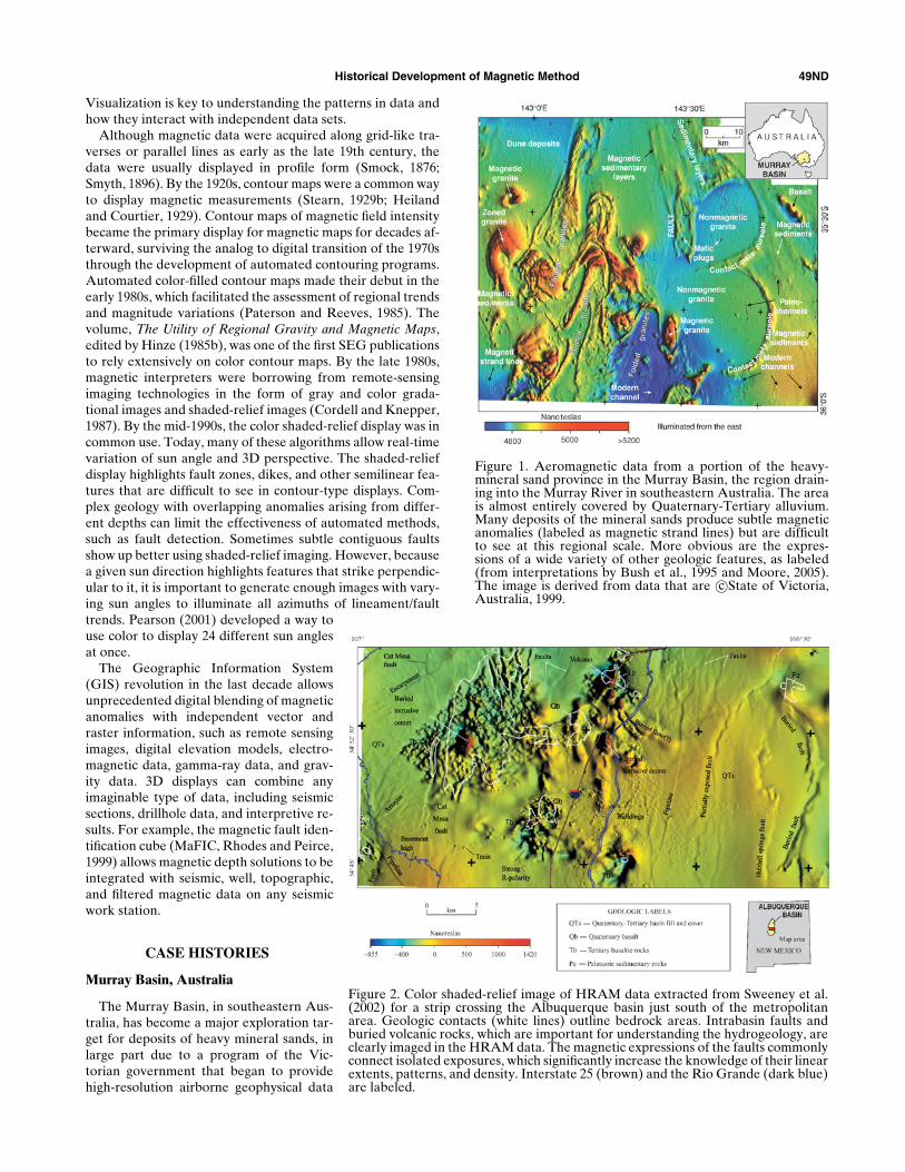
Historical Development of Magnetic Method 49ND
Visualization is key to understanding the patterns in data andhow they interact with independent data sets.
Although magnetic data were acquired along grid-like tra-verses or parallel lines as early as the late 19th century, thedata were usually displayed in profile form (Smock, 1876;Smyth, 1896). By the 1920s, contour maps were a common wayto display magnetic measurements (Stearn, 1929b; Heilandand Courtier, 1929). Contour maps of magnetic field intensitybecame the primary display for magnetic maps for decades af-terward, surviving the analog to digital transition of the 1970sthrough the development of automated contouring programs.Automated color-filled contour maps made their debut in theearly 1980s, which facilitated the assessment of regional trendsand magnitude variations (Paterson and Reeves, 1985). Thevolume, The Utility of Regional Gravity and Magnetic Maps,edited by Hinze (1985b), was one of the first SEG publicationsto rely extensively on color contour maps. By the late 1980s,magnetic interpreters were borrowing from remote-sensingimaging technologies in the form of gray and color grada-tional images and shaded-relief images (Cordell and Knepper,1987). By the mid-1990s, the color shaded-relief display was incommon use. Today, many of these algorithms allow real-timevariation of sun angle and 3D perspective. The shaded-reliefdisplay highlights fault zones, dikes, and other semilinear fea-tures that are difficult to see in contour-type displays. Com-plex geology with overlapping anomalies arising from differ-ent depths can limit the effectiveness of automated methods,such as fault detection. Sometimes subtle contiguous faultsshow up better using shaded-relief imaging. However, becausea given sun direction highlights features that strike perpendic-ular to it, it is important to generate enough images with vary-ing sun angles to illuminate all azimuths of lineament/faulttrends. Pearson (2001) developed a way touse color to display 24 different sun anglesat once.
The Geographic Information System(GIS) revolution in the last decade allowsunprecedented digital blending of magneticanomalies with independent vector andraster information, such as remote sensingimages, digital elevation models, electro-magnetic data, gamma-ray data, and grav-ity data. 3D displays can combine anyimaginable type of data, including seismicsections, drillhole data, and interpretive re-sults. For example, the magnetic fault iden-tification cube (MaFIC, Rhodes and Peirce,1999) allows magnetic depth solutions to beintegrated with seismic, well, topographic,and filtered magnetic data on any seismicwork station.
CASE HISTORIES
Murray Basin, Australia
The Murray Basin, in southeastern Aus-tralia, has become a major exploration tar-get for deposits of heavy mineral sands, inlarge part due to a program of the Vic-torian government that began to providehigh-resolution airborne geophysical data
Figure 1. Aeromagnetic data from a portion of the heavy-mineral sand province in the Murray Basin, the region drain-ing into the Murray River in southeastern Australia. The areais almost entirely covered by Quaternary-Tertiary alluvium.Many deposits of the mineral sands produce subtle magneticanomalies (labeled as magnetic strand lines) but are difficultto see at this regional scale. More obvious are the expres-sions of a wide variety of other geologic features, as labeled(from interpretations by Bush et al., 1995 and Moore, 2005).The image is derived from data that are c©State of Victoria,Australia, 1999.
Figure 2. Color shaded-relief image of HRAM data extracted from Sweeney et al.(2002) for a strip crossing the Albuquerque basin just south of the metropolitanarea. Geologic contacts (white lines) outline bedrock areas. Intrabasin faults andburied volcanic rocks, which are important for understanding the hydrogeology, areclearly imaged in the HRAM data. The magnetic expressions of the faults commonlyconnect isolated exposures, which significantly increase the knowledge of their linearextents, patterns, and density. Interstate 25 (brown) and the Rio Grande (dark blue)are labeled.
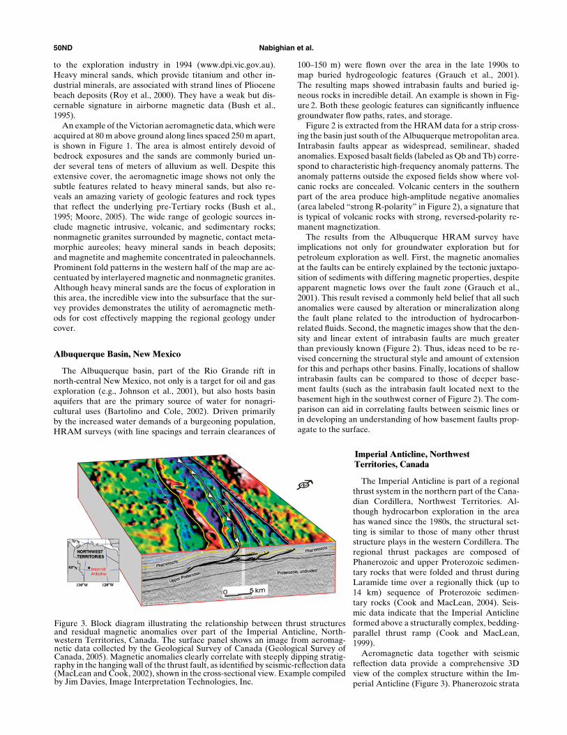
50ND Nabighian et al.
to the exploration industry in 1994 (www.dpi.vic.gov.au).Heavy mineral sands, which provide titanium and other in-dustrial minerals, are associated with strand lines of Pliocenebeach deposits (Roy et al., 2000). They have a weak but dis-cernable signature in airborne magnetic data (Bush et al.,1995).
An example of the Victorian aeromagnetic data, which wereacquired at 80 m above ground along lines spaced 250 m apart,is shown in Figure 1. The area is almost entirely devoid ofbedrock exposures and the sands are commonly buried un-der several tens of meters of alluvium as well. Despite thisextensive cover, the aeromagnetic image shows not only thesubtle features related to heavy mineral sands, but also re-veals an amazing variety of geologic features and rock typesthat reflect the underlying pre-Tertiary rocks (Bush et al.,1995; Moore, 2005). The wide range of geologic sources in-clude magnetic intrusive, volcanic, and sedimentary rocks;nonmagnetic granites surrounded by magnetic, contact meta-morphic aureoles; heavy mineral sands in beach deposits;and magnetite and maghemite concentrated in paleochannels.Prominent fold patterns in the western half of the map are ac-centuated by interlayered magnetic and nonmagnetic granites.Although heavy mineral sands are the focus of exploration inthis area, the incredible view into the subsurface that the sur-vey provides demonstrates the utility of aeromagnetic meth-ods for cost effectively mapping the regional geology undercover.
Albuquerque Basin, New Mexico
The Albuquerque basin, part of the Rio Grande rift innorth-central New Mexico, not only is a target for oil and gasexploration (e.g., Johnson et al., 2001), but also hosts basinaquifers that are the primary source of water for nonagri-cultural uses (Bartolino and Cole, 2002). Driven primarilyby the increased water demands of a burgeoning population,HRAM surveys (with line spacings and terrain clearances of
Figure 3. Block diagram illustrating the relationship between thrust structuresand residual magnetic anomalies over part of the Imperial Anticline, North-western Territories, Canada. The surface panel shows an image from aeromag-netic data collected by the Geological Survey of Canada (Geological Survey ofCanada, 2005). Magnetic anomalies clearly correlate with steeply dipping stratig-raphy in the hanging wall of the thrust fault, as identified by seismic-reflection data(MacLean and Cook, 2002), shown in the cross-sectional view. Example compiledby Jim Davies, Image Interpretation Technologies, Inc.
100–150 m) were flown over the area in the late 1990s tomap buried hydrogeologic features (Grauch et al., 2001).The resulting maps showed intrabasin faults and buried ig-neous rocks in incredible detail. An example is shown in Fig-ure 2. Both these geologic features can significantly influencegroundwater flow paths, rates, and storage.
Figure 2 is extracted from the HRAM data for a strip cross-ing the basin just south of the Albuquerque metropolitan area.Intrabasin faults appear as widespread, semilinear, shadedanomalies. Exposed basalt fields (labeled as Qb and Tb) corre-spond to characteristic high-frequency anomaly patterns. Theanomaly patterns outside the exposed fields show where vol-canic rocks are concealed. Volcanic centers in the southernpart of the area produce high-amplitude negative anomalies(area labeled “strong R-polarity” in Figure 2), a signature thatis typical of volcanic rocks with strong, reversed-polarity re-manent magnetization.
The results from the Albuquerque HRAM survey haveimplications not only for groundwater exploration but forpetroleum exploration as well. First, the magnetic anomaliesat the faults can be entirely explained by the tectonic juxtapo-sition of sediments with differing magnetic properties, despiteapparent magnetic lows over the fault zone (Grauch et al.,2001). This result revised a commonly held belief that all suchanomalies were caused by alteration or mineralization alongthe fault plane related to the introduction of hydrocarbon-related fluids. Second, the magnetic images show that the den-sity and linear extent of intrabasin faults are much greaterthan previously known (Figure 2). Thus, ideas need to be re-vised concerning the structural style and amount of extensionfor this and perhaps other basins. Finally, locations of shallowintrabasin faults can be compared to those of deeper base-ment faults (such as the intrabasin fault located next to thebasement high in the southwest corner of Figure 2). The com-parison can aid in correlating faults between seismic lines orin developing an understanding of how basement faults prop-agate to the surface.
Imperial Anticline, NorthwestTerritories, Canada
The Imperial Anticline is part of a regionalthrust system in the northern part of the Cana-dian Cordillera, Northwest Territories. Al-though hydrocarbon exploration in the areahas waned since the 1980s, the structural set-ting is similar to those of many other thruststructure plays in the western Cordillera. Theregional thrust packages are composed ofPhanerozoic and upper Proterozoic sedimen-tary rocks that were folded and thrust duringLaramide time over a regionally thick (up to14 km) sequence of Proterozoic sedimen-tary rocks (Cook and MacLean, 2004). Seis-mic data indicate that the Imperial Anticlineformed above a structurally complex, bedding-parallel thrust ramp (Cook and MacLean,1999).
Aeromagnetic data together with seismicreflection data provide a comprehensive 3Dview of the complex structure within the Im-perial Anticline (Figure 3). Phanerozoic strata
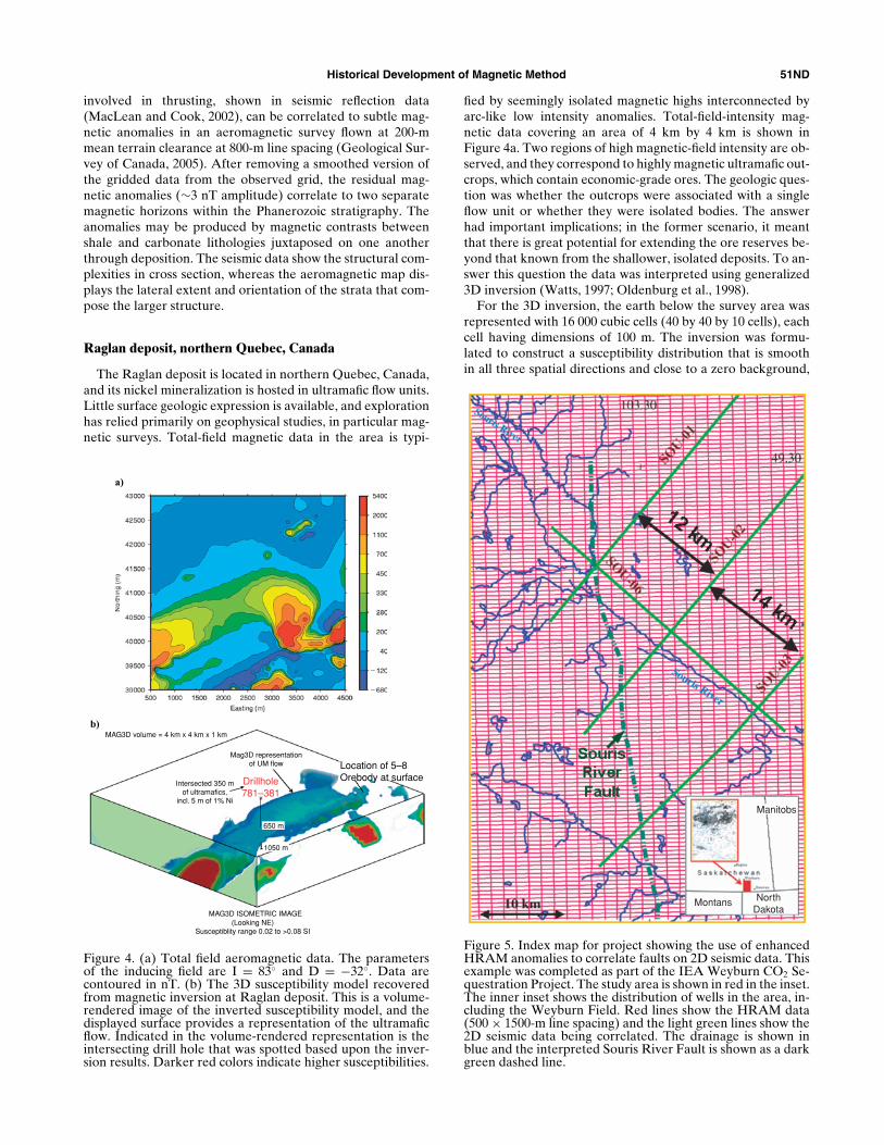
Historical Development of Magnetic Method 51ND
involved in thrusting, shown in seismic reflection data(MacLean and Cook, 2002), can be correlated to subtle mag-netic anomalies in an aeromagnetic survey flown at 200-mmean terrain clearance at 800-m line spacing (Geological Sur-vey of Canada, 2005). After removing a smoothed version ofthe gridded data from the observed grid, the residual mag-netic anomalies (∼3 nT amplitude) correlate to two separatemagnetic horizons within the Phanerozoic stratigraphy. Theanomalies may be produced by magnetic contrasts betweenshale and carbonate lithologies juxtaposed on one anotherthrough deposition. The seismic data show the structural com-plexities in cross section, whereas the aeromagnetic map dis-plays the lateral extent and orientation of the strata that com-pose the larger structure.
Raglan deposit, northern Quebec, Canada
The Raglan deposit is located in northern Quebec, Canada,and its nickel mineralization is hosted in ultramafic flow units.Little surface geologic expression is available, and explorationhas relied primarily on geophysical studies, in particular mag-netic surveys. Total-field magnetic data in the area is typi-
a)
−
−
Mag3D representationof UM flow Location of 5–8
Orebody at surfaceDrillhole781–381
Intersected 350 mof ultramafics,
incl. 5 m of 1% Ni
1050 m
650 m
MAG3D ISOMETRIC IMAGE(Looking NE)
Susceptiblity range 0.02 to >0.08 SI
b)MAG3D volume = 4 km x 4 km x 1 km
Figure 4. (a) Total field aeromagnetic data. The parametersof the inducing field are I = 83◦ and D = −32◦. Data arecontoured in nT. (b) The 3D susceptibility model recoveredfrom magnetic inversion at Raglan deposit. This is a volume-rendered image of the inverted susceptibility model, and thedisplayed surface provides a representation of the ultramaficflow. Indicated in the volume-rendered representation is theintersecting drill hole that was spotted based upon the inver-sion results. Darker red colors indicate higher susceptibilities.
fied by seemingly isolated magnetic highs interconnected byarc-like low intensity anomalies. Total-field-intensity mag-netic data covering an area of 4 km by 4 km is shown inFigure 4a. Two regions of high magnetic-field intensity are ob-served, and they correspond to highly magnetic ultramafic out-crops, which contain economic-grade ores. The geologic ques-tion was whether the outcrops were associated with a singleflow unit or whether they were isolated bodies. The answerhad important implications; in the former scenario, it meantthat there is great potential for extending the ore reserves be-yond that known from the shallower, isolated deposits. To an-swer this question the data was interpreted using generalized3D inversion (Watts, 1997; Oldenburg et al., 1998).
For the 3D inversion, the earth below the survey area wasrepresented with 16 000 cubic cells (40 by 40 by 10 cells), eachcell having dimensions of 100 m. The inversion was formu-lated to construct a susceptibility distribution that is smoothin all three spatial directions and close to a zero background,
Montans
Manitobs
NorthDakota
Figure 5. Index map for project showing the use of enhancedHRAM anomalies to correlate faults on 2D seismic data. Thisexample was completed as part of the IEA Weyburn CO2 Se-questration Project. The study area is shown in red in the inset.The inner inset shows the distribution of wells in the area, in-cluding the Weyburn Field. Red lines show the HRAM data(500 × 1500-m line spacing) and the light green lines show the2D seismic data being correlated. The drainage is shown inblue and the interpreted Souris River Fault is shown as a darkgreen dashed line.
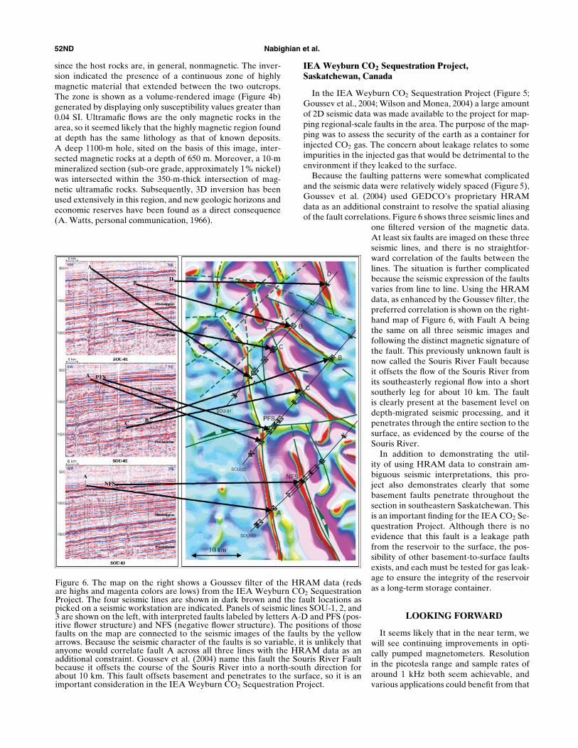
52ND Nabighian et al.
since the host rocks are, in general, nonmagnetic. The inver-sion indicated the presence of a continuous zone of highlymagnetic material that extended between the two outcrops.The zone is shown as a volume-rendered image (Figure 4b)generated by displaying only susceptibility values greater than0.04 SI. Ultramafic flows are the only magnetic rocks in thearea, so it seemed likely that the highly magnetic region foundat depth has the same lithology as that of known deposits.A deep 1100-m hole, sited on the basis of this image, inter-sected magnetic rocks at a depth of 650 m. Moreover, a 10-mmineralized section (sub-ore grade, approximately 1% nickel)was intersected within the 350-m-thick intersection of mag-netic ultramafic rocks. Subsequently, 3D inversion has beenused extensively in this region, and new geologic horizons andeconomic reserves have been found as a direct consequence(A. Watts, personal communication, 1966).
Figure 6. The map on the right shows a Goussev filter of the HRAM data (redsare highs and magenta colors are lows) from the IEA Weyburn CO2 SequestrationProject. The four seismic lines are shown in dark brown and the fault locations aspicked on a seismic workstation are indicated. Panels of seismic lines SOU-1, 2, and3 are shown on the left, with interpreted faults labeled by letters A-D and PFS (pos-itive flower structure) and NFS (negative flower structure). The positions of thosefaults on the map are connected to the seismic images of the faults by the yellowarrows. Because the seismic character of the faults is so variable, it is unlikely thatanyone would correlate fault A across all three lines with the HRAM data as anadditional constraint. Goussev et al. (2004) name this fault the Souris River Faultbecause it offsets the course of the Souris River into a north-south direction forabout 10 km. This fault offsets basement and penetrates to the surface, so it is animportant consideration in the IEA Weyburn CO2 Sequestration Project.
IEA Weyburn CO2 Sequestration Project,Saskatchewan, Canada
In the IEA Weyburn CO2 Sequestration Project (Figure 5;Goussev et al., 2004; Wilson and Monea, 2004) a large amountof 2D seismic data was made available to the project for map-ping regional-scale faults in the area. The purpose of the map-ping was to assess the security of the earth as a container forinjected CO2 gas. The concern about leakage relates to someimpurities in the injected gas that would be detrimental to theenvironment if they leaked to the surface.
Because the faulting patterns were somewhat complicatedand the seismic data were relatively widely spaced (Figure 5),Goussev et al. (2004) used GEDCO’s proprietary HRAMdata as an additional constraint to resolve the spatial aliasingof the fault correlations. Figure 6 shows three seismic lines and
one filtered version of the magnetic data.At least six faults are imaged on these threeseismic lines, and there is no straightfor-ward correlation of the faults between thelines. The situation is further complicatedbecause the seismic expression of the faultsvaries from line to line. Using the HRAMdata, as enhanced by the Goussev filter, thepreferred correlation is shown on the right-hand map of Figure 6, with Fault A beingthe same on all three seismic images andfollowing the distinct magnetic signature ofthe fault. This previously unknown fault isnow called the Souris River Fault becauseit offsets the flow of the Souris River fromits southeasterly regional flow into a shortsoutherly leg for about 10 km. The faultis clearly present at the basement level ondepth-migrated seismic processing, and itpenetrates through the entire section to thesurface, as evidenced by the course of theSouris River.
In addition to demonstrating the util-ity of using HRAM data to constrain am-biguous seismic interpretations, this pro-ject also demonstrates clearly that somebasement faults penetrate throughout thesection in southeastern Saskatchewan. Thisis an important finding for the IEA CO2 Se-questration Project. Although there is noevidence that this fault is a leakage pathfrom the reservoir to the surface, the pos-sibility of other basement-to-surface faultsexists, and each must be tested for gas leak-age to ensure the integrity of the reservoiras a long-term storage container.
LOOKING FORWARD
It seems likely that in the near term, wewill see continuing improvements in opti-cally pumped magnetometers. Resolutionin the picotesla range and sample rates ofaround 1 kHz both seem achievable, andvarious applications could benefit from that
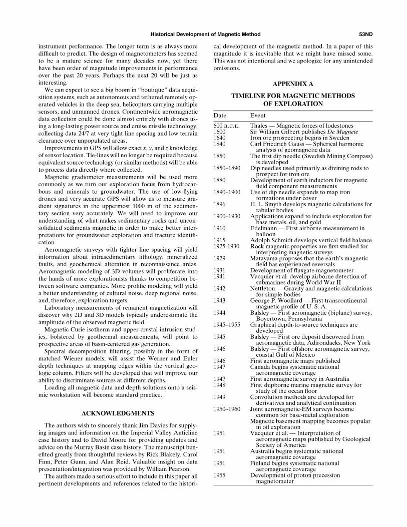
Historical Development of Magnetic Method 53ND
instrument performance. The longer term is as always moredifficult to predict. The design of magnetometers has seemedto be a mature science for many decades now, yet therehave been order of magnitude improvements in performanceover the past 20 years. Perhaps the next 20 will be just asinteresting.
We can expect to see a big boom in “boutique” data acqui-sition systems, such as autonomous and tethered remotely op-erated vehicles in the deep sea, helicopters carrying multiplesensors, and unmanned drones. Continentwide aeromagneticdata collection could be done almost entirely with drones us-ing a long-lasting power source and cruise missile technology,collecting data 24/7 at very tight line spacing and low terrainclearance over unpopulated areas.
Improvements in GPS will allow exact x, y, and z knowledgeof sensor location. Tie-lines will no longer be required becauseequivalent source technology (or similar methods) will be ableto process data directly where collected.
Magnetic gradiometer measurements will be used morecommonly as we turn our exploration focus from hydrocar-bons and minerals to groundwater. The use of low-flyingdrones and very accurate GPS will allow us to measure gra-dient signatures in the uppermost 1000 m of the sedimen-tary section very accurately. We will need to improve ourunderstanding of what makes sedimentary rocks and uncon-solidated sediments magnetic in order to make better inter-pretations for groundwater exploration and fracture identifi-cation.
Aeromagnetic surveys with tighter line spacing will yieldinformation about intrasedimentary lithology, mineralizedfaults, and geochemical alteration in reconnaissance areas.Aeromagnetic modeling of 3D volumes will proliferate intothe hands of more explorationists thanks to competition be-tween software companies. More prolific modeling will yielda better understanding of cultural noise, deep regional noise,and, therefore, exploration targets.
Laboratory measurements of remanent magnetization willdiscover why 2D and 3D models typically underestimate theamplitude of the observed magnetic field.
Magnetic Curie isotherm and upper-crustal intrusion stud-ies, bolstered by geothermal measurements, will point toprospective areas of basin-centered gas generation.
Spectral decomposition filtering, possibly in the form ofmatched Wiener models, will assist the Werner and Eulerdepth techniques at mapping edges within the vertical geo-logic column. Filters will be developed that will improve ourability to discriminate sources at different depths.
Loading all magnetic data and depth solutions onto a seis-mic workstation will become standard practice.
ACKNOWLEDGMENTS
The authors wish to sincerely thank Jim Davies for supply-ing images and information on the Imperial Valley Anticlinecase history and to David Moore for providing updates andadvice on the Murray Basin case history. The manuscript ben-efited greatly from thoughtful reviews by Rick Blakely, CarolFinn, Peter Gunn, and Alan Reid. Valuable insight on datapresentation/integration was provided by William Pearson.
The authors made a serious effort to include in this paper allpertinent developments and references related to the histori-
cal development of the magnetic method. In a paper of thismagnitude it is inevitable that we might have missed some.This was not intentional and we apologize for any unintendedomissions.
APPENDIX A
TIMELINE FOR MAGNETIC METHODSOF EXPLORATION
Date Event
600 B.C.E. Thales — Magnetic forces of lodestones1600 Sir William Gilbert publishes De Magnete1640 Iron ore prospecting begins in Sweden1840 Carl Friedrich Gauss — Spherical harmonic
analysis of geomagnetic data1850 The first dip needle (Swedish Mining Compass)
is developed1850–1890 Dip needles used primarily as divining rods to
prospect for iron ore1880 Development of earth inductors for magnetic
field component measurements1890–1900 Use of dip needle expands to map iron
formations under cover1896 H. L. Smyth develops magnetic calculations for
tabular bodies1900–1930 Applications expand to include exploration for
base metals, oil, and gold1910 Edelmann — First airborne measurement in
balloon1915 Adolph Schmidt develops vertical field balance1925-1930 Rock magnetic properties are first studied for
interpreting magnetic surveys1929 Matayama proposes that the earth’s magnetic
field has experienced reversals1931 Development of fluxgate magnetometer1941 Vacquier et al. develop airborne detection of
submarines during World War II1942 Nettleton — Gravity and magnetic calculations
for simple bodies1943 George P. Woollard — First transcontinental
magnetic profile of U. S. A.1944 Balsley — First aeromagnetic (biplane) survey,
Boyertown, Pennsylvania1945–1955 Graphical depth-to-source techniques are
developed1945 Balsley — First ore deposit discovered from
aeromagnetic data, Adirondacks, New York1946 Balsley — First offshore aeromagnetic survey,
coastal Gulf of Mexico1946 First aeromagnetic maps published1947 Canada begins systematic national
aeromagnetic coverage1947 First aeromagnetic survey in Australia1948 First shipborne marine magnetic survey for
study of the ocean floor1949 Convolution methods are developed for
derivatives and analytical continuation1950–1960 Joint aeromagnetic-EM surveys become
common for base-metal explorationMagnetic basement mapping becomes popular
in oil exploration1951 Vacquier et al. — Interpretation of
aeromagnetic maps published by GeologicalSociety of America
1951 Australia begins systematic nationalaeromagnetic coverage
1951 Finland begins systematic nationalaeromagnetic coverage
1955 Development of proton precessionmagnetometer
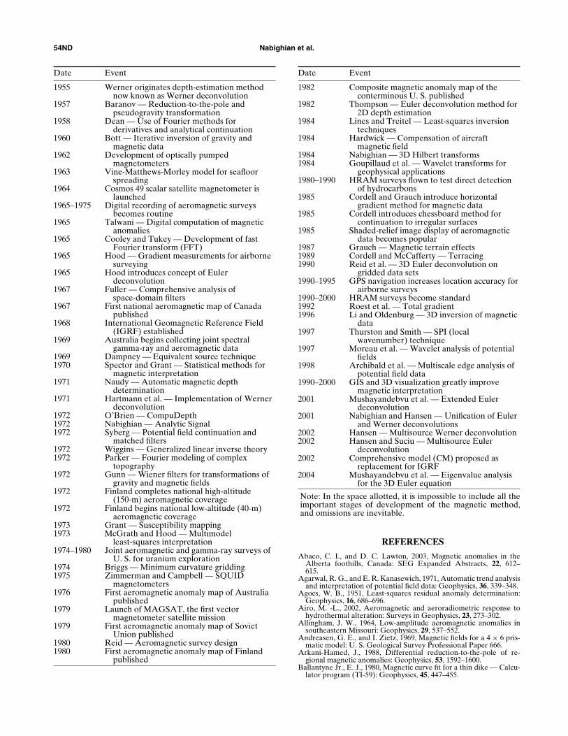
54ND Nabighian et al.
Date Event
1955 Werner originates depth-estimation methodnow known as Werner deconvolution
1957 Baranov — Reduction-to-the-pole andpseudogravity transformation
1958 Dean — Use of Fourier methods forderivatives and analytical continuation
1960 Bott — Iterative inversion of gravity andmagnetic data
1962 Development of optically pumpedmagnetometers
1963 Vine-Matthews-Morley model for seafloorspreading
1964 Cosmos 49 scalar satellite magnetometer islaunched
1965–1975 Digital recording of aeromagnetic surveysbecomes routine
1965 Talwani — Digital computation of magneticanomalies
1965 Cooley and Tukey — Development of fastFourier transform (FFT)
1965 Hood — Gradient measurements for airbornesurveying
1965 Hood introduces concept of Eulerdeconvolution
1967 Fuller — Comprehensive analysis ofspace-domain filters
1967 First national aeromagnetic map of Canadapublished
1968 International Geomagnetic Reference Field(IGRF) established
1969 Australia begins collecting joint spectralgamma-ray and aeromagnetic data
1969 Dampney — Equivalent source technique1970 Spector and Grant — Statistical methods for
magnetic interpretation1971 Naudy — Automatic magnetic depth
determination1971 Hartmann et al. — Implementation of Werner
deconvolution1972 O’Brien — CompuDepth1972 Nabighian — Analytic Signal1972 Syberg — Potential field continuation and
matched filters1972 Wiggins — Generalized linear inverse theory1972 Parker — Fourier modeling of complex
topography1972 Gunn — Wiener filters for transformations of
gravity and magnetic fields1972 Finland completes national high-altitude
(150-m) aeromagnetic coverage1972 Finland begins national low-altitude (40-m)
aeromagnetic coverage1973 Grant — Susceptibility mapping1973 McGrath and Hood — Multimodel
least-squares interpretation1974–1980 Joint aeromagnetic and gamma-ray surveys of
U. S. for uranium exploration1974 Briggs — Minimum curvature gridding1975 Zimmerman and Campbell — SQUID
magnetometers1976 First aeromagnetic anomaly map of Australia
published1979 Launch of MAGSAT, the first vector
magnetometer satellite mission1979 First aeromagnetic anomaly map of Soviet
Union published1980 Reid — Aeromagnetic survey design1980 First aeromagnetic anomaly map of Finland
published
Date Event
1982 Composite magnetic anomaly map of theconterminous U. S. published
1982 Thompson — Euler deconvolution method for2D depth estimation
1984 Lines and Treitel — Least-squares inversiontechniques
1984 Hardwick — Compensation of aircraftmagnetic field
1984 Nabighian — 3D Hilbert transforms1984 Goupillaud et al. — Wavelet transforms for
geophysical applications1980–1990 HRAM surveys flown to test direct detection
of hydrocarbons1985 Cordell and Grauch introduce horizontal
gradient method for magnetic data1985 Cordell introduces chessboard method for
continuation to irregular surfaces1985 Shaded-relief image display of aeromagnetic
data becomes popular1987 Grauch — Magnetic terrain effects1989 Cordell and McCafferty — Terracing1990 Reid et al. — 3D Euler deconvolution on
gridded data sets1990–1995 GPS navigation increases location accuracy for
airborne surveys1990–2000 HRAM surveys become standard1992 Roest et al. — Total gradient1996 Li and Oldenburg — 3D inversion of magnetic
data1997 Thurston and Smith — SPI (local
wavenumber) technique1997 Moreau et al. — Wavelet analysis of potential
fields1998 Archibald et al. — Multiscale edge analysis of
potential field data1990–2000 GIS and 3D visualization greatly improve
magnetic interpretation2001 Mushayandebvu et al. — Extended Euler
deconvolution2001 Nabighian and Hansen — Unification of Euler
and Werner deconvolutions2002 Hansen — Multisource Werner deconvolution2002 Hansen and Suciu — Multisource Euler
deconvolution2002 Comprehensive model (CM) proposed as
replacement for IGRF2004 Mushayandebvu et al. — Eigenvalue analysis
for the 3D Euler equation
Note: In the space allotted, it is impossible to include all theimportant stages of development of the magnetic method,and omissions are inevitable.
REFERENCES
Abaco, C. I., and D. C. Lawton, 2003, Magnetic anomalies in theAlberta foothills, Canada: SEG Expanded Abstracts, 22, 612–615.
Agarwal, R. G., and E. R. Kanasewich, 1971, Automatic trend analysisand interpretation of potential field data: Geophysics, 36, 339–348.
Agocs, W. B., 1951, Least-squares residual anomaly determination:Geophysics, 16, 686–696.
Airo, M. -L., 2002, Aeromagnetic and aeroradiometric response tohydrothermal alteration: Surveys in Geophysics, 23, 273–302.
Allingham, J. W., 1964, Low-amplitude aeromagnetic anomalies insoutheastern Missouri: Geophysics, 29, 537–552.
Andreasen, G. E., and I. Zietz, 1969, Magnetic fields for a 4 × 6 pris-matic model: U. S. Geological Survey Professional Paper 666.
Arkani-Hamed, J., 1988, Differential reduction-to-the-pole of re-gional magnetic anomalies: Geophysics, 53, 1592–1600.
Ballantyne Jr., E. J., 1980, Magnetic curve fit for a thin dike — Calcu-lator program (TI-59): Geophysics, 45, 447–455.
Historical Development of Magnetic Method 55ND
Balsley, J. R., 1952, Aeromagnetic surveying, in H. E. Landsberg, ed.,Advances in Geophysics, 1: Academic Press, 313–350.
Baranov, V., 1957, A new method for interpretation of aeromagneticmaps pseudo-gravimetric anomalies: Geophysics, 22, 359–383.
Baranov, V., and H. Naudy, 1964, Numerical calculation of theformula of reduction to the magnetic pole: Geophysics, 29,67–79.
Barbosa, V. C. F., J. B. C. Silva, and W. E. Medeiros, 1999, Stabilityanalysis and improvement of structural index estimation in Eulerdeconvolution: Geophysics, 64, 48–60.
Barnett, C. T., 1976, Theoretical modeling of the magnetic and grav-itational fields of an arbitrarily shaped three-dimensional body:Geophysics, 41, 1353–1364.
Barongo, J. O., 1985, Method for depth estimation and aeromagneticvertical gradient anomalies: Geophysics, 50, 963–968.
Bartolino, J. R., and J. C. Cole, 2002, Ground-water resources of theMiddle Rio Grande Basin, New Mexico: U. S. Geological SurveyCircular 1222.
Barton, C. E., 1997, International Geomagnetic Reference Field: Theseventh generation: Journal of Geomagnetism and Geoelectricity,49, 123–148.
Batchelor, A., and J. Gutmanis, 2002, Hydrocarbon production fromfractured basement reservoirs — version 7: www.geoscience.co.uk/downloads/fracturedbasementver7.pdf.
Bath, G. D., 1968, Aeromagnetic anomalies related to remanent mag-netism in volcanic rock, Nevada Test Site: Geological Society ofAmerica Memoir 110, 135–146.
Bath, G. D. and C. E. Jahren, 1984, Interpretation of magnetic anoma-lies at a potential repository site located in the Yucca Mountainarea, Nevada Test Site: U. S. Geological Survey Open File Report84–120.
Bean, R. J., W. F. Fillippone, N. R. Paterson, and I. Zietz, 1961, Dis-cussion of “An evaluation of basement depth determination fromairborne magnetometer data,” by Peter Jacobsen Jr.: Geophysics,26, 317–319.
Bhattacharyya, B. K., 1964, Magnetic anomalies due to prism-shapedbodies with arbitrary polarization: Geophysics, 29, 517–531.
———, 1965, Two-dimensional harmonic analysis as a tool for mag-netic interpretation: Geophysics, 30, 829–857.
———, 1966, Continuous spectrum of the total-magnetic-fieldanomaly due to a rectangular prismatic body: Geophysics, 31, 97–121.
———, 1969, Bicubic spline interpolation as a method for treatmentof potential field data: Geophysics, 34, 402–423.
———, 1980, A generalized multibody model for inversion of mag-netic anomalies: Geophysics, 45, 255–270.
Bhattacharyya, B. K., and K. C. Chan, 1977a, Reduction of magneticand gravity data on an arbitrary surface acquired in a region of hightopographic relief: Geophysics, 42, 1411–1430.
———, 1977b, Computation of gravity and magnetic anomalies dueto inhomogeneous distribution of magnetization and density in alocalized region: Geophysics, 42, 602–609.
Blakely, R. J., 1981, A program for rapidly computing the magneticanomaly over digital topography: U. S. Geological Survey OpenFile Report 81–298.
———, 1995, Potential theory in gravity and magnetic applications:Cambridge University Press.
Blakely, R. J., and V. J. S. Grauch, 1983, Magnetic models of crys-talline terrane; accounting for the effect of topography: Geophysics,48, 1551–1557.
Blakely, R. J., and S. Hassanzadeh, 1981, Estimation of depth to mag-netic source using maximum entropy power spectra, with applica-tion to the Peru-Chile Trench, Nazca Plate; Crustal formation andAndean convergence: Geological Society of America Memoir 154,667–682.
Blakely, R. J., and R. W. Simpson, 1986, Approximating edges ofsource bodies from magnetic or gravity anomalies: Geophysics, 51,1494–1498.
Blakely, R. J., V. E. Langenheim, D. A. Ponce, and G. L. Dixon,2000a, Aeromagnetic survey of the Amargosa Desert, Nevadaand California; a tool for understanding near-surface geology andhydrology: U. S. Geological Survey Open File Report 00-0188,http://pubs.usgs.gov/open-file/of00-188/.
Blakely, R. J., R. E. Wells, T. L. Tolan, M. H. Beeson, A. M. Trehu,and L. M. Liberty, 2000b, New aeromagnetic data reveal largestrike-slip faults in the northern Willamette Valley, Oregon: Ge-ological Society of America Bulletin, 112, 1225–1233.
Boardman, J. W., 1985, Magnetic anomalies over oil fields: M.S. thesis,Colorado School of Mines.
Books, K. G., 1962, Remanent magnetism as a contributor to someaeromagnetic anomalies: Geophysics, 27, 359–375.
Bott, M. H. P., 1960, The use of rapid digital computing meth-ods for direct gravity interpretation of sedimentary basins:
Geophysical Journal of the Royal Astronomical Society, 3,63–67.
———, 1963, Two methods applicable to computers for evaluatingmagnetic anomalies due to finite three dimensional bodies: Geo-physical Prospecting, 11, 292–299.
Breiner, S., 1981, Horizontal gradient methods for airborne and ma-rine geophysical exploration: 51st Annual International Meeting,SEG, Expanded Abstracts, Geophysics, 441–442.
Briggs, I. C., 1974, Machine contouring using minimum curvature:Geophysics, 39, 39–48.
Broding, R. A., C. W. Zimmerman, E. V. Somers, E. S. Wilhelm,and A. A. Stripling, 1952, Magnetic well-logging: Geophysics, 17,1–26.
Bush, M. D., R. A. Cayley, S. Rooney, K. Slater, and M. L. Whitehead,1995, The geology and prospectivity of the southern margin of theMurray Basin: Geological Survey of Victoria VIMP Report 4.
Butler, D. K., 2001, Potential fields methods for location of unex-ploded ordnance: The Leading Edge, 20, 890–895.
Byerly, P. E., 1965, Convolution filtering of gravity and magneticmaps: Geophysics, 30, 281–283.
Cady, J. W., 1980, Calculation of gravity and magnetic anomalies offinite-length right polygonal prisms: Geophysics, 45, 1507–1512.
Campbell, W. C., 1997, Introduction to geomagnetic fields: CambridgeUniversity Press.
Campos-Enriquez, J. O., R. Diaz-Navarro, J. M. Espindola, andM. Mena, 1996, Chicxulub — Subsurface structure of impact craterinferred from gravity and magnetic data: The Leading Edge, 15,357–359.
Chapin, D. A., 1997, Wavelet transforms: A new paradigm for in-terpreting gravity and magnetics data?: 67th Annual InternationalMeeting, SEG, Expanded Abstracts, 486–489.
Chapin, D. A., S. V. Yalamanchili, and P. H. Daggett, 1998, The St.George Basin, Alaska, COST #1 well: An example of the need forintegrated interpretation, in R. I. Gibson, and P. S. Millegan, eds.,Geologic applications of gravity and magnetics: Case histories: SEGand AAPG.
Clark, D. A., 1983, Comments on magnetic petrophysics: Bulletin ofAustralian Society of Exploration Geophysicists, 14, 49–62.
———, 1997, Magnetic petrophysics and magnetic petrology; aids togeological interpretation of magnetic surveys: AGSO Journal ofAustralian Geology and Geophysics, 17, 83–103.
Clark, D. A., and D. W. Emerson, 1991, Notes on rock magneti-zation characteristics in applied geophysical studies: ExplorationGeophysics, 22, 547–555.
Clarke, G. K. C., 1969, Optimum second derivative and downwardcontinuation filters: Geophysics, 34, 424–437.
Committee for the Magnetic Anomaly Map of North America, 1987,Magnetic anomaly map of North America: Geological Society ofAmerica Continent Scale Map 003.
Cook, D. G., and B. C. MacLean, 1999: The Imperial Anticline,a fault-bend fold above a bedding-parallel thrust ramp, North-west Territories, Canada: Journal of Structural Geology, 21,215–228.
———, 2004: Subsurface Proterozoic stratigraphy and tectonics of thewestern plains of the Northwest Territories. Geological Survey ofCanada, Bulletin 575.
Cooper, G. R. J., and D. R. Cowan, 2003, Sunshading geophysical datausing fractional order horizontal gradients: The Leading Edge, 22,204.
Cordell, L., 1979, Gravimetric expression of graben faulting in SantaFe County and the Espanola Basin, New Mexico, in R. V. Ingersoll,ed., Guidebook to Santa Fe County: 30th Field Conference, NewMexico Geological Society, 59–64.
———, 1985a, Applications and problems of analytical continuationof New Mexico aeromagnetic data between arbitrary surfaces ofvery high relief: Proceedings of International Meeting on PotentialFields in Rugged Topography, Institut de Geophysique de Univer-site de Lausanne, Bulletin 7, 96–101
———, 1985b, A stripping filter for potential field data: SEG, Ex-panded Abstracts, 55th Annual International Meeting, SEG, Ex-panded Abstracts, 217–218.
———, 1992, A scattered equivalent-source method for the interpola-tion and gridding of potential-field data in three dimensions: Geo-physics, 57, 629–636.
Cordell, L., and V. J. S. Grauch, 1982, Mapping basement magneti-zation zones from aeromagnetic data in the San Juan Basin, NewMexico: 52nd Annual International Meeting, SEG, Expanded Ab-stracts, 246–247.
———, 1985, Mapping basement magnetization zones from aero-magnetic data in the San Juan Basin New Mexico, in W. J.Hinze, ed., Utility of regional gravity and magnetic maps: SEG,181–197.
Cordell, L., and D. H. Knepper, 1987, Aeromagnetic images: Fresh in-
56ND Nabighian et al.
sight to the buried basement, Rolla quadrangle, southeast Missouri:Geophysics, 52, 218–231.
Cordell, L., and A. E. McCafferty, 1989, A terracing operator forphysical property mapping with potential field data: Geophysics, 54,621–634.
Cowan, D. R., and S. Cowan, 1993, Separation filtering applied toaeromagnetic data: Exploration Geophysics, 24, 429–436.
Cox, A., 1973, Plate tectonics and geomagnetic reversals: W. H. Free-man and Company.
Craig, M., 1996, Analytic signals for multivariate data: MathematicalGeology, 28, 315–329.
Cribb, J., 1976, Application of the generalized linear inverse to theinversion of static potential data: Geophysics, 41, 1365–1369.
Davies, J., M. F. Mushayandebvu, and R. Smith, 2004, Magnetic de-tection and characterization of Tertiary and Quaternary buriedchannels: 74th Annual International Meeting, SEG, Expanded Ab-stracts, 734.
Dean, W. C., 1958, Frequency analysis for gravity and magnetic inter-pretation: Geophysics, 23, 97–127.
Dickinson, M., 1986, A search for intra-sedimentary aeromagneticanomalies over a known oil field in the Denver Basin: M.S. thesis,Colorado School of Mines.
Dietz, R. S., 1961, Continent and ocean basin evolution by spreadingof the sea floor: Nature, 190, 854–857.
Eaton, D., and K. Vasudevan, 2004, Skeletonization of aeromagneticdata: Geophysics, 69, 478–488.
EG&G Geometrics (ca.1970s), A guide to passive magnetic com-pensation of aircrafts: EG&G Geometrics Technical ReportNumber 15.
Fairhead, J. D., J. D. Misener, C. M. Green, G. Bainbridge, and S. W.Reford, 1997, Large scale compilations of magnetic, gravity, radio-metric and electromagnetic data: The new exploration strategy forthe 90s, in A. G. Gubins, ed., Proceedings of Exploration 97: FourthDecennial International Conference on Mineral Exploration,805–816.
Finn, C. A., ed., 2002, Examples of the utility of magnetic anomalydata for geologic mapping: U. S. Geological Survey Open-file Re-port 02-0400, available at http://pubs.usgs.gov/of/2002/ofr-02-0400/
Finn, C. A., T. W. Sisson, and M. Deszcz-Pan, 2001, Aerogeophysicalmeasurements of collapse-prone hydrothermally altered zones atMount Rainier Volcano: Nature, 409, 600–603.
Finn, C. A., and L. A. Morgan, 2002, High-resolution aeromagneticmapping of volcanic terrain, Yellowstone National Park: Journal ofVolcanology and Geothermal Research, 115, 207–231.
Fitzgerald, D., A. Reid, and P. McInerney, 2003, New discriminationtechniques for Euler deconvolution: 8th South African GeophysicalAssociation (SAGA) Biennial Technical Meeting and Exhibition.
Frischknecht, F. C., L. Muth, R. Grette, T. Buckley, and B. Korne-gay, 1983, Geophysical methods for locating abandoned wells: U. S.Geological Survey Open File Report 83–702.
Frowe, E., 1948, A total field magnetometer for mobile operation:Geophysics, 13, 209–214.
Fuller, B. D., 1967, Two-dimensional frequency analysis and designof grid operators, in Mining Geophysics, II: Society of ExplorationGeophysicists, 658–708.
Gay Jr., S. P., 1992, Epigenetic versus syngenetic magnetite as a causeof magnetic anomalies: Geophysics, 57, 60–68.
———, 2004, Glacial till: A troublesome source of near-surface mag-netic anomalies: The Leading Edge, 23, 542–547.
Gay, S. P., and B. W. Hawley, 1991, Syngenetic magnetic anomalysources: Three examples: Geophysics, 56, 902–913.
Geological Survey of Canada, 2005, Canadian Aeromagnetic DataBase, Central Canada Division, Earth Sciences Sector, Natural Re-sources Canada.
Gerovska, D., and M. J. Arauzo-Bravo, 2003, Automatic interpreta-tion of magnetic data based on Euler deconvolution with unpre-scribed structural index: Computers & Geosciences, 29, 949–960.
Gibson, R. I., and P. S. Millegan, eds., 1998, Geologic applications ofgravity and magnetics: Case histories: SEG and AAPG.
Goldhaber, M. B., and R. L. Reynolds, 1991, Relations among hydro-carbon reservoirs, epigenetic sulfidization, and rock magnetization:Examples from the south Texas coastal plain: Geophysics, 56, 748–757.
Goupillaud, P. L., A. Grossmann, and J. Morlet, 1984, Cycle-octaveand related transforms in seismic signal analysis: Geoexploration,23, 85–102.
Goussev, S. A., R. A. Charters, J. W. Peirce, and W. E. Glenn, 2003,Jackpine magnetic anomaly: Identification of a buried meteorite im-pact structure: The Leading Edge, 22, 740–741.
Goussev, S. A., L. Griffith, J. Peirce, and A. Cordsen, 2004, EnhancedHRAM anomalies correlate faults between 2D seismic lines: 74thAnnual International Meeting, SEG, Extended Abstracts, 730.
Grant, F. S., 1972, Review of data processing and interpreta-
tion methods in gravity and magnetics, 1964–71: Geophysics, 37,647–661.
Grant, F. S., 1973, The magnetic susceptibility mapping method for in-terpreting aeromagnetic surveys: 43rd Annual International Meet-ing, SEG, Expanded Abstracts, 1201.
———, 1985, Aeromagnetics, geology and ore environments, inMagnetite in igneous, sedimentary and metamorphic rocks: Anoverview: Geoexploration, 23, 303–333.
Grant, F. S., and L. Martin, 1966, Interpretation of aeromagneticanomalies by the use of characteristic curves: Geophysics, 31,135–148.
Grauch, V. J. S., 1987, A new variable-magnetization terrain correc-tion method for aeromagnetic data: Geophysics, 52, 94–107.
Grauch, V. J. S., and L. Cordell, 1987, Limitations on determiningdensity or magnetic boundaries from the horizontal gradient ofgravity or pseudogravity data: Geophysics, 52, 118–121.
Grauch, V. J. S., and C. S. Johnston, 2002, Gradient window method:A simple way to separate regional from local horizontal gradientsin gridded potential-field data: 72nd Annual International Meeting,SEG, Expanded Abstracts, 762–765.
Grauch, V. J. S., D. A. Sawyer, C. J. Fridrich, and M. R. Hudson,1999, Geophysical framework of the southwestern Nevada volcanicfield and hydrogeologic implications: U. S. Geological Survey Pro-fessional Paper1608.
Grauch, V. J. S., M. R. Hudson, and S. A. Minor, 2001, Aeromagneticexpression of faults that offset basin fill, Albuquerque basin, NewMexico: Geophysics, 66, 707–720.
Griffin, W. R., 1949, Residual gravity in theory and practice: Geo-physics, 14, 39–56.
Grivet, P. A., and L. Malnar, 1967, Measurement of weak magneticfields by magnetic resonance: Advances in Electronics and ElectronPhysics, 23, 39–151.
Guillen, A., and V. Menichetti, 1984, Gravity and magnetic inversionwith minimization of a specific functional: Geophysics, 49, 1354–1360.
Gunn, P. J., 1972, Application of Wiener filters to transforma-tions of gravity and magnetic fields: Geophysical Prospecting, 20,860–871.
———, 1975, Linear transformations of gravity and magnetic fields:Geophysical Prospecting, 23, 300–312.
———, 1995, An algorithm for reduction to the pole that works at allmagnetic latitudes: Exploration Geophysics, 26, 247–254.
———, 1997, Application of aeromagnetic surveys to sedimentarybasin studies: AGSO Journal of Australian Geology and Geo-physics, 17, 133–144.
———, 1998, Aeromagnetics locates prospective areas and prospects:The Leading Edge, 17, 67–69.
Gunn, P. J., D. FitzGerald, and N. Yassi, 1996, Complex attributes:New tools for enhancing aeromagnetic data: Australian Geolog-ical Survey Organization (AGSO) Research Newsletter, no. 25,16–17.
Guspi, F., and B. Introcaso, 2000, A sparse spectrum technique forgridding and separating potential field anomalies: Geophysics, 65,1154–1161.
Haggerty, S. E., 1979, The aeromagnetic mineralogy of igneous rocks:Canadian Journal of Earth Sciences, 16, 1281–1293.
Hall, S. H., 1962, The modulation of a proton magnetometer signaldue to rotation: Geophysical Journal, 7, 131–142.
Hammer, S., 1963, Deep gravity interpretation by stripping: Geo-physics, 28, 369–378.
Haney, M., and Y. Li, 2002, Total magnetization direction and dipfrom multiscale edge: 72nd Annual International Meeting, SEG,Expanded Abstracts, 735–738.
Haney, M., C. Johnston, Y. Li, and M. Nabighian, 2003, Envelopes of2D and 3D magnetic data and their relationship to the analytic sig-nal: Preliminary results: 73rd Annual International Meeting, SEGExpanded Abstracts, 596–599.
Hanna, W. F., 1990, Some historical notes on early magnetic surveyingin the U. S. Geological Survey, in W. F. Hanna, ed., Geologic appli-cations of modern aeromagnetic surveys: U. S. Geological SurveyBulletin 1924, 63–73.
Hansen, R. O., 1984, Two approaches to total field reconstructionfrom gradiometer data: 54th Annual International Meeting, SEGExpanded Abstracts, 245.
———, 1993, Interpretative gridding by anisotropic kriging: Geo-physics, 58, 1491–1497.
———, 2002, 3D multiple-source Werner deconvolution: 72nd An-nual International Meeting, SEG, Expanded Abstracts, 802–805.
Hansen, R. O., and Y. Miyazaki, 1984, Continuation of potential fieldsbetween arbitrary surfaces: Geophysics, 49, 787–795.
Hansen, R. O., and R. S. Pawlowski, 1989, Reduction-to-the-pole at low latitudes by Wiener filtering: Geophysics, 54, 1607–1613.
Historical Development of Magnetic Method 57ND
Hansen, R. O., and M. Simmonds, 1993, Multiple-source Werner de-convolution: Geophysics, 58, 1792–1800.
Hansen, R. O., and L. Suciu, 2002, Multiple-source Euler deconvolu-tion: Geophysics, 67, 525–535.
Hardwick, C. D., 1984, Important design considerations for inboardairborne magnetic gradiometers: Geophysics, 49, 2004–2018.
Hartman, R. R., D. J. Teskey, and J. L. Friedberg, 1971, A sys-tem for rapid digital aeromagnetic interpretation: Geophysics, 36,891–918.
Hassan, H. H., and J. W. Peirce, 2005, SAUCE: A new technique toremove cultural noise from HRAM: The Leading Edge, 24, 246–250.
Hassan, H. H., J. W. Peirce, W. C. Pearson, and M. J. Pearson, 1998,Cultural editing of HRAM data: Comparison of techniques: Cana-dian Journal of Exploration Geophysics, 34, www.cseg.ca.
Heezen, B. C., M. Ewing, and E. T. Miller, 1953, Trans-Atlantic pro-file of total magnetic intensity and topography: Dakar to Barbados:Deep Sea Research, 1, 25–23.
Heiland, C. A., 1935, Geophysical mapping from the air: Its possibili-ties and advantages: Engineering and Mining Journal, 136, 609–610.
———, 1940, Geophysical Exploration: Prentice Hall.Heiland, C. A., and W. H. Courtier, 1929, Magnetometric investiga-
tion and gold placer deposits near Golden (Jefferson County), Col-orado: Transactions of the American Institute of Mining, Metallur-gical and Petroleum Engineers (AIME), 81, 364–384.
Henderson, R., 1960, A comprehensive system of automatic compu-tation in magnetic and gravity interpretation: Geophysics, 25, 569–585.
Henderson, R. G., and I. Zietz, 1948, Analysis of total magnetic inten-sity anomalies produced by point and line sources: Geophysics, 13,428–436.
———, 1949, The computation of second vertical derivatives of geo-magnetic fields: Geophysics, 14, 508–516.
Hess, H. H., 1962, History of ocean basins, in A. E. J. Engel, H. L.James, and B. F. Leonard, eds., Petrologic studies: A volume tohonor A. F. Buddington: Geological Society of America, 599–620.
Hildenbrand, T. G., and G. . Raines, 1990, Need for aeromagneticdata and a national airborne geophysics program: U. S. GeologicalSurvey Bulletin 1924, 1–5.
Hinze, W. J., 1985a, ed., Proceedings of the International Meeting onPotential Fields in Rugged Topography: Institut de Geophysiquede Universite de Lausanne, Bulletin no. 7.
———, 1985b, ed., The utility of regional gravity and magneticanomaly maps: SEG, 181–197.
Hjelt, S. E., 1972, Magnetostatic anomalies of a dipping prism: Geo-exploration, 10, 239–254.
Hogg, R. L. S., 1979, Illustration of a new Northway process for elim-inating the “herringbone” component from problem geophysicaldata: Annual Meeting of Canadian Society of Exploration Geo-physicists.
Holstein, H., 2002a, Gravimagnetic similarity in anomaly formulas foruniform polyhedra: Geophysics, 67, 1126–1133.
Holstein, H., 2002b, Invariance in gravimagnetic anomaly formulasfor uniform polyhedra: Geophysics, 67, 1134–1137.
Hood, P. J., 1990, Aeromagnetic survey program of Canada, mineralapplications, and vertical gradiometry, in W. F. Hanna, ed., Geo-logic applications of modern aeromagnetic surveys: U. S. Geologi-cal Survey Bulletin 1924, 7–23.
Hornby, P., F. Boschetti, and F. G. Horowitz, 1999, Analysis of poten-tial field data in the wavelet domain: Geophysical Journal Interna-tional, 137, 175–196.
Hoylman, H. W., 1961, How to determine and remove diurnal effectsprecisely: World Oil, December, 107–112.
Huang, D., and P. A. Versnel, 2000, Depth estimation algorithm ap-plied to FTG data: 70th Annual International Meeting, SEG, Ex-panded Abstracts, 394–397.
Hutchison, R. D., 1958, Magnetic analysis by logarithmic curves: Geo-physics, 23, 749–769.
Jacobsen, B., 1987, A case for upward continuation as a stan-dard separation filter for potential-field maps: Geophysics, 52,1138–1148.
Jacobson Jr., P., 1961, An evaluation of basement depth determina-tions from airborne magnetometer data: Geophysics, 26, 309–317.
Jain, S., 1976, An automatic method of direct interpretation of mag-netic profiles: Geophysics, 41, 531–545.
Jakosky, J. J., 1950, Exploration geophysics: Trija Publishing Com-pany.
Jenny, W. P., 1936, Micromagnetic surveys: Gulf Coast structures maybe outlined by this new method: The Oil Weekly, April 27.
Jensen, H., 1965, Instrument details and application of a new airbornemagnetometer: Geophysics, 30, 875–882.
Jessell, M. W., 2001, Three-dimensional modeling of potential-fielddata: Computers & Geosciences, 27, 455–465.
Jessell, M. W., and Fractal Geophysics Pty Ltd., 2002, An atlasof structural geophysics II: Journal of the Virtual Explorer, 5,http://www.mssu.edu/seg-vm/exhibits/structuraatlas/index.html.
Jessell, M. W., and R. K. Valenta, 1996, Structural geophysics: In-tegrated structural and geophysical mapping, in D. DePaor, ed.,Structural geology and personal computers: Elsevier Science Pub-lishing Co., 303–324.
Jessell, M. W., R. K. Valenta, G. Jung, J. P. Cull, and A. Gerio, 1993,Structural geophysics: Exploration Geophysics, 24, 599–602.
Johnson, R. C., T.M. Finn, and V. F. Nuccio, 2001, Potential for abasin-centered gas accumulation in the Albuquerque Basin, NewMexico: U. S. Geological Survey Bulletin 2184-C, available onlineat http://pubs.usgs.gov/bul/b2184-c/.
Josephson, B. D., 1962, Possible new effect in superconductive tun-neling: Physics Letters, 1, 251–253.
Keating, P., 1993, The fractal dimension of gravity data sets and itsimplication for gridding: Geophysical Prospecting, 41, 983–994.
———, 1995, A simple technique to identify magnetic anomalies dueto kimberlite pipes: Exploration Mining Geology, 4, 121–125.
Keating, P., and M. Pilkington, 2000, Euler deconvolution of the an-alytic signal: 62nd Annual International Meeting, EAGE, SessionP0193.
Keating, P., and L. Zerbo, 1996, An improved technique for reductionto the pole at low latitudes: Geophysics, 61, 131–137.
Kellogg, O. D., 1953, Foundations of potential theory: Dover Publica-tions.
Kilty, K. T., 1983, Werner deconvolution of profile potential field data:Geophysics, 48, 234–237.
Korhonen, J. V., H. Saavuori, and T. Koistinen, 2003, Petrophysicalcorrelation of Fennoscandian magnetic and gravity anomalies: Eu-ropean Geophysical Society (EGS) –American Geophysical Union(AGU)–European Union of Geosciences (EUG) Joint Assembly,abstract #13230.
Koulomzine, T., Y. Lamontagne, and A. Nadeau, 1970, New meth-ods for the direct interpretation of magnetic anomalies caused byinclined dikes of infinite length: Geophysics, 35, 812–830.
Ku, C. C., and J. A. Sharp, 1983, Werner deconvolution for automatedmagnetic interpretation and its refinement using Marquardt inversemodeling: Geophysics, 48, 754–774.
Langel, R. A., 1992, International Geomagnetic Reference Field: Thesixth generation: Journal of Geomagnetism and Geoelectricity, 44,679–707.
Langel, R. A., and W. J. Hinze, 1998, The magnetic field of the Earth’slithosphere: The satellite perspective: Cambridge University Press.
Langenheim, V. E., R. C. Jachens, D. M. Morton, R. W. Kistler, andJ. C. Matti, 2004, Geophysical and isotopic mapping of preexistingcrustal structures that influenced the location and development ofthe San Jacinto fault zone, southern California: Geological Societyof America Bulletin, 116, 1143–1157.
Leblanc, G., and W. A. Morris, 2001, Denoising of aeromagnetic datavia the wavelet transform: Geophysics, 66, 1793–1804.
Leliak, P., 1961, Identification and evaluation of magnetic-fieldsources of magnetic airborne detector equipped aircraft: IRETransactions on Aerospace and Navigational Electronics, 8,95–106.
Leu, L., 1982, Use of reduction-to-the-equator process for magneticdata interpretation: Geophysics, 47, 445
Levanto, A. E., 1959, A three-component magnetometer for smalldrill holes and its use in ore prospecting: Geophysical Prospecting,7, 183–195
Li, Y., and D. W. Oldenburg, 1996, 3-D inversion of magnetic data:Geophysics, 61, 394–408.
———, 1998a, Separation of regional and residual magnetic field data:Geophysics, 63, 431–439.
———, 1998b, Stable reduction to the pole at the magnetic equa-tor: 68th Annual International Meeting, SEG, Expanded Abstracts,533–536.
———, 1999, Rapid construction of equivalent sources using wavelets:60th Annual International Meeting, SEG, Expanded Abstracts,374–377.
———, 2000a, Reduction to the pole using equivalent sources: 60thAnnual International Meeting, SEG, Expanded Abstracts, 386–389.
———, 2000b, Joint inversion of surface and three-component bore-hole magnetic data: Geophysics, 65, 540–552.
———, 2003, Fast inversion of large-scale magnetic data using wavelettransforms and logarithmic barrier method: Geophysical JournalInternational, 152, 251–265.
Logachev, A. A., 1946, The development and application of airbornemagnetometers in the U.S.S.R.: Geophysics, 11, 135–147.
Lundberg, H., 1947, Results obtained by a helicopter borne magne-tometer: Transactions, Canadian Institute of Mining and Metal-lurgy, 50, 392–400.
58ND Nabighian et al.
Macdonald, K. C., S. P. Miller, S. P. Huestis, and F. N. Spiess, 1980,Three-dimensional modeling of a magnetic reversal boundary frominversion of deep-tow measurements: Journal of Geophysical Re-search, 85, 3670–3680.
Machel, H. G., and E. A. Burton, 1991, Chemical and microbial pro-cesses causing anomalous magnetization in environments affectedby hydrocarbon seepage: Geophysics, 56, 598–605.
MacLean, B. C., and D. G. Cook, 2002(updated), Subsurface and sur-face distribution of Proterozoic units, northwestern NWT: a Cam-brian sub-crop map: Geological Survey of Canada, Open File 3502.
Macmillan, S., S. Maus, T. Bondar, A. Chambodut, V. Golovkov,R. Holme, B. Langlais et al., 2003, Ninth generation InternationalGeomagnetic Reference Field released: EOS Transactions of theAmerican Geophysical Union, 84, 503.
Macnae, J. C., 1979, Kimberlites and exploration geophysics: Geo-physics, 44, 1395–1416.
Mason, R. G., 1958, A magnetic survey off the west coast of theUnited States between latitudes 30◦ and 36◦ N, longitudes 121◦ and128◦ W: Geophysical Journal of the Royal Astronomical Society, 1,320–329.
Maus, S., 1999, Variogram analysis of magnetic and gravity data: Geo-physics, 64, 776–784.
Maus, S., K. P. Sengpiel, B. Rottger, and E. A. W. Tordiffe, 1999, Var-iogram analysis of helicopter magnetic data to identify paleochan-nels of the Omaruru River, Namibia: Geophysics, 64, 785–794.
Maus, S., and S. Macmillan, 2005, 10th generation International Geo-magnetic Reference Field: EOS Transactions of the American Geo-physical Union, 86, 159.
Maxwell, A. E., R. P. von Herzen, et al., 1970, Initial Reports ofthe Deep Sea Drilling Project; covering Leg 3 of the cruises ofthe drilling vessel “Glomar Challenger,” Dakar, Senegal to Rio deJaneiro, Brazil, December 1968 to January 1969: Deep Sea DrillingProject: U. S. Government Printing Office.
Mazur, M. J., R. R. Stewart, and A. R. Hildebrand, 2000, The seismicsignature of meteorite impact craters: Canadian Society of Explo-ration Geophysicists Recorder, 35, June, 10–16.
McConnell, T. J., B. Lo, A. Ryder-Turner, and J. A. Musser, 1999,Enhanced 3D seismic surveys using a new airborne pipeline map-ping system: 69th Annual International Meeting, SEG, ExpandedAbstracts, 516–519.
McElhinny, M. W., 1973, Paleomagnetics and plate tectonics: Cam-bridge University Press.
McIntyre, J. I., 1980, Geological significance of magnetic patterns re-lated to magnetite in sediments and metasediments — A review:Bulletin of the Australian Society of Exploration Geophysicists, 11,19–33.
Mendonca, C. A., and J. B. C. Silva, 1993, A stable truncated seriesapproximation of the reduction-to-the-pole operator: Geophysics,58, 1084–1090.
———, 1994, The equivalent data concept applied to the interpolationof potential-field data: Geophysics, 59, 722–732.
———, 1995, Interpolation of potential-field data by equivalent layerand minimum curvature: A comparative analysis: Geophysics, 60,399–407.
Mesko, A., 1965, Some notes concerning the frequency analysis forgravity interpretation: Geophysical Prospecting, 13, 475–488.
Millegan, P. S., 1998, High-resolution aeromagnetic surveying, inR. I. Gibson, and P. S. Millegan, eds., Geologic applications of grav-ity and magnetics: Case histories: SEG and AAPG.
Miller, H. G., and V. Singh, 1994, Potential field tilt; a new concept forlocation of potential field sources: Journal of Applied Geophysics,32, 213–217.
Minty, B. R. S., 1991, Simple microlevelling for aeromagnetic data:Exploration Geophysics, 22, 591–592.
Misener, D. J., F. S. Grant, and P. Walker, 1984, Variable depth,space-domain magnetic susceptibility mapping: 54th Annual Inter-national Meeting, SEG, Expanded Abstracts, 237.
Mittal, P. K., 1984, Algorithm for error adjustment of potential-fielddata along a survey network: Geophysics, 49, 467–469.
Modisi, M. P., E. A. Atekwana, A. B. Kampunzu, and T. H. Ng-wisanyi, 2000, Rift kinematics during the incipient stages of con-tinental extension: Evidence from the nascent Okavango rift basin,northwest Botswana: Geology, 28, 939–942.
Moore, D. H., 2005, Swan Hill 1:250,000 and parts of Balranald andDeniliquin 1:250,000 map areas: A geological interpretation of thegeophysical data: Victorian Initiative for Minerals and PetroleumReport 84, Department of Primary Industries, Victoria, Australia.
Moreau, F., D. Gibert, M. Holschneider, and G. Saracco, 1997,Wavelet analysis of potential fields: Inverse Problems, 13, 165–178.
Morgan, R., 1998, Magnetic anomalies associated with the North andSouth Morecambe Fields, U. K., in R. I. Gibson, and P. R. Milligan,eds., Geologic applications of gravity and magnetics: Case histories:SEG and AAPG, 89–91.
Morley, L. W., 1963, The geophysics division of the Geological Surveyof Canada: Bulletin of the Canadian Institute of Mining Metallurgy,5, 358–364.
———, 2001, The zebra pattern, in N. Orestes, ed., Plate tectonics:An insider’s history of the modern theory of the Earth: WestviewPress, 67–85.
Morley, L. W., and A. Larochelle, 1964, Paleomagnetism as a meansof dating geological events: Royal Society of Canada Special Publi-cation 8, 39–50.
Mushayandebvu, M., A. Reid, and D. Fairhead, 2000, Grid Euler de-convolution with constraints for 2-D structures: 70th Annual Inter-national Meeting, SEG, Expanded Abstracts, 398–401.
Mushayandebvu, M. F., P. van Driel, A. B. Reid, and J. D.Fairhead, 2001, Magnetic source parameters of two-dimensionalstructures using extended Euler deconvolution: Geophysics, 66,814–823.
Mushayandebvu, M. F., V. Lesur, A. B. Reid, and J. D. Fairhead, 2004,Grid Euler deconvolution with constraints for 2D structures: Geo-physics, 69, 489–496.
Nabighian, M. N., 1972, The analytic signal of two-dimensionalmagnetic bodies with polygonal cross-section — Its propertiesand use for automated anomaly interpretation: Geophysics, 37,507–517.
———, 1974, Additional comments on the analytic signal of two-dimensional magnetic bodies with polygonal cross-section: Geo-physics, 39, 85–92.
———, 1984, Toward a three-dimensional automatic interpretationof potential field data via generalized Hilbert transforms — Funda-mental relations: Geophysics, 49, 780–786.
Nabighian, M. N., and R. O. Hansen, 2001, Unification of Eulerand Werner deconvolution in three dimensions via the generalizedHilbert transform: Geophysics, 66, 1805–1810.
Naudy, H., 1971, Automatic determination of depth on aeromagneticprofiles: Geophysics, 36, 717–722.
Naudy, H., and H. Dreyer, 1968, Essai de filtrage non-lineaire ap-plique aux profiles aeromagnetiques (Attempt to apply nonlinearfiltering to aeromagnetic profiles): Geophysical Prospecting, 16,171–178.
Nettleton, L. L., 1942, Gravity and magnetic calculations: Geophysics,7, 293–310.
———, 1971, Elementary gravity and magnetics for geologists andseismologists: SEG.
North American Magnetic Anomaly Group, 2002, Magnetic anomalymap of North America: U. S. Geological Survey Special Map, avail-able online at http://pubs.usgs.gov/sm/mag map/.
O’Brien, D. P., 1972, CompuDepth, a new method for depth-to-basement computation: Presented at the 42nd Annual InternationalMeeting, SEG.
O’Connell, M. D., 2001, A heuristic method of removing micropul-sations from airborne magnetic data: The Leading Edge, 20, 1242–1244.
O’Connell, M. D., R. S. Smith, and M. A. Vallee, 2005, Gridding aero-magnetic data using longitudinal and transverse gradients with theminimum curvature operator: The Leading Edge, 24, 142–145.
Okabe, M., 1979, Analytical expressions for gravity anomalies dueto homogeneous polyhedral bodies and translations into magneticanomalies: Geophysics, 44, 730–741.
Oldenburg, D. W., Y. Li, C. G. Farquharson, P. Kowalczyk, T. Ara-vanis, A. King, P. Zhang, and A. Watts, 1998, Applications of geo-physical inversions in mineral exploration: The Leading Edge, 17,461–465.
Olsen, N., R. Holm, G. Hulot, T. Sabaka, T. Neubert, L. Tøffner-Clausen, F. Primdahl, et al., 2000, Ørsted initial field model: Geo-physical Research Letters, 27, 3607.
Oreskes, N., 2001, Plate tectonics: An insider’s history of the moderntheory of the Earth: Westview Press.
Parker, R. L., 1972, The rapid calculation of potential anomalies: Geo-physical Journal of the Royal Astronomical Society, 31, 447–455.
Parker, R. L., and S. P. Huestis, 1974, Inversion of magnetic anomaliesin the presence of topography: Journal of Geophysical Research,79, 1587–1593.
Parker, R. L., and K. D. Klitgord, 1972, Magnetic upward continua-tion from an uneven track: Geophysics, 37, 662–668.
Paterson, N. R., and C. V. Reeves, 1985, Applications of gravity andmagnetic surveys — The state of the art in 1985: Geophysics, 50,2558–2594.
Pawlowski, R. S., and R. O. Hansen, 1990, Gravity anomaly separa-tion by Wiener filtering: Geophysics, 55, 539–548.
Pearson, W. C., 1996, Removing culture from southern Texas — Amagnetic clean-up and imaging revolution: 66th Annual Interna-tional Meeting, SEG, Expanded Abstracts, 1407–1410.
———, 2001, Finding faults in a gas play: AAPG Explorer, May,52–55.
Historical Development of Magnetic Method 59ND
Pearson, W. C., and C. M. Skinner, 1982, Reduction-to-the-pole of lowlatitude magnetic anomalies: 52nd Annual International Meeting,SEG, Expanded Abstracts, 356.
Peddie, N. W., 1982, International Geomagnetic Reference Field: Thethird generation: Journal of Geomagnetism and Geoelectricity, 34,309–326.
———, 1983, International Geomagnetic Reference Field — Its evo-lution and the difference in total field intensity between new andold models for 1965–1980: Geophysics, 48, 1691–1696.
Pedersen, L. B., 1977, Interpretation of potential field data — A gen-eralized inverse approach: Geophysical Prospecting, 25, 199–230.
———, 1978, Wavenumber domain expressions for potential fieldsfrom arbitrary 2-, 2 1
2 -, and 3-dimensional bodies: Geophysics, 43,626–630.
———, 1979, Constrained inversion of potential field data: Geophys-ical Prospecting, 27, 726–748.
Peirce, J. W., W. E. Glenn, and K. Brown, eds., 1998, High resolutionaeromagnetics for hydrocarbon exploration: Canadian Journal ofExploration Geophysics, 34, available online at www.cseg.ca.
Peirce, J. W., S. A. Goussev, R. McLean, and M. Marshall, 1999,Aeromagnetic interpretation of the Dianango Trough HRAM sur-vey, onshore Gabon: 69th Annual International Meeting, SEG, Ex-tended Abstracts, 343–346.
Peters, L. J., 1949, The direct approach to magnetic interpretation andits practical application: Geophysics, 14, 290–320.
Phillips, J. D., 1979, ADEPT, A program to estimate depth to mag-netic basement from sampled magnetic profiles: U. S. GeologicalSurvey Open File Report No. 79-367.
———, 2000, Locating magnetic contacts: A comparison of the hor-izontal gradient, analytic signal, and local wavenumber methods:70th Annual International Meeting, SEG, Expanded Abstracts,402–405.
———, 2001, Designing matched bandpass and azimuthal filters forthe separation of potential-field anomalies by source region andsource type: 15th Geophysical Conference and Exhibition, Aus-tralian Society of Exploration Geophysicists, Expanded Abstracts,CD-ROM.
———, 2002, Two-step processing for 3D magnetic source locationsand structural indices using extended Euler or analytic signal meth-ods: 72nd Annual International Meeting, SEG, Expanded Ab-stracts, 727–730.
Phillips, J. D., R. W. Saltus, and R. L. Reynolds, 1998, Sources of mag-netic anomalies over a sedimentary basin: Preliminary results fromthe Coastal Plain of the Arctic National Wildlife Refuge, Alaska,in R. I. Gibson and P. S. Millegan, eds., Geologic applications ofgravity and magnetics: Case histories: SEG and AAPG, 130–134.
Pilkington, M., 1997, 3-D magnetic imaging using conjugate gradients:Geophysics, 62, 1132–1142.
Pilkington, M., and D. J. Crossley, 1986, Determination of crustalinterface topography from potential fields: Geophysics, 51, 1277–1284.
Pilkington, M., and P. Keating, 2004, Contact mapping from griddedmagnetic data — A comparison of techniques: Exploration Geo-physics, 35, 306–311.
Pilkington, M., M. E. Gregotski, and J. P. Todoeschuck, 1994, Us-ing fractal crustal magnetization models in magnetic interpretation:Geophysical Prospecting, 42, 677–692.
Plouff, D., 1975, Derivation of formulas and FORTRAN programs tocompute magnetic anomalies of prisms: National Technical Infor-mation Service No. PB-243-525, U. S. Department of Commerce.
———, 1976, Gravity and magnetic fields of polygonal prisms and ap-plication to magnetic terrain corrections: Geophysics, 41, 727–741.
Power, M., G. Belcourt, and E. Rockel, 2004, Geophysical methodsfor kimberlite exploration in northern Canada: The Leading Edge,23, 1124
Prieto, C., and G. Morton, 2003, New insights from a 3D earth model,deepwater Gulf of Mexico: The Leading Edge, 22, 356–360.
Pustisek, A. M., 1990, Noniterative three-dimensional inversion ofmagnetic data: Geophysics, 55, 782–785.
Rasmussen, R., and L. B. Pedersen, 1979, End corrections in potentialfield modeling: Geophysical Prospecting, 27, 749–760.
Ravat, D., T. G. Hildenbrand, and W. Roest, 2003, New way of pro-cessing near-surface magnetic data: The utility of the Comprehen-sive Model of the magnetic field: The Leading Edge, 22, 784–785.
Reford, M. S., 1980, History of geophysical exploration — Magneticmethod: Geophysics, 45, 1640–1658.
Reford, M. S., and J. S. Sumner, 1964, Aeromagnetics: Geophysics,29, 482–516.
Reid, A. B., 1980, Aeromagnetic survey design: Geophysics, 45, 973–976.
Reid, A. B., J. M. Allsop, H. Granser, A. J. Millett, and I. W. Somer-ton, 1990, Magnetic interpretation in three dimensions using Eulerdeconvolution: Geophysics, 55, 80–91.
Reigber, C., H. Luehr, and P. Schwintzer, 2002, CHAMP mission sta-tus: Advances in Space Research, 30, 289–293.
Reynolds, R. L., J. G. Rosenbaum, M. R. Hudson, and N. S. Fishman,1990, Rock magnetism, the distribution of magnetic minerals in theEarth’s crust, and aeromagnetic anomalies: U. S. Geological SurveyBulletin1924, 24–45.
Reynolds, R. L., M. Webring, V. J. S. Grauch, and M. Tuttle, 1990,Magnetic forward models of Cement oil field, Oklahoma, based onrock magnetic, geochemical and petrologic constraints: Geophysics,55, 344–353.
Reynolds, R. L., N. S. Fishman, and M. R. Hudson, 1991, Sources ofaeromagnetic anomalies over Cement oil field (Oklahoma), Simp-son oil field (Alaska), and the Wyoming-Idaho-Utah thrust belt:Geophysics, 56, 606–617.
Rhodes, J., and J. W. Peirce, 1999, MaFIC — Magnetic interpreta-tion in 3-D using a seismic workstation: 69th Annual InternationalMeeting, SEG, Expanded Abstracts, 335–338.
Ridsdill-Smith, T. A., 1998a, Separating aeromagnetic anomalies us-ing wavelet matched filters: 68th Annual International Meeting,SEG, Expanded Abstracts, 550–553.
———, 1998b, Separation filtering of aeromagnetic data using filter-banks: Exploration Geophysics, 29, 577–583.
———, 2000, Wavelet compression of an equivalent layer: 70th An-nual International Meeting, SEG, Expanded Abstracts, 378–381.
Ridsdill-Smith, T. A., and M. C. Dentith, 1999, The wavelet transformin aeromagnetic processing: Geophysics, 64, 1003–1013.
Robson, D. F., and R. Spencer, 1997, The New South Wales govern-ment’s Discovery 2000 — Geophysical surveys and their effect onexploration: Exploration Geophysics, 28, 296–298.
Roest, W. R., and M. Pilkington, 1993, Identifying remanent magneti-zation effects in magnetic data: Geophysics, 58, 653–659.
Roest, W. R., J. Verhoef, and M. Pilkington, 1992, Magnetic interpre-tation using the 3D analytic signal: Geophysics, 57, 116–125.
Rosenbaum, J. G., and D. B. Snyder, 1985, Preliminary interpretationof paleomagnetic and magnetic property data from drill holes USWG-1, G-2, GU-3, G-3, and VH-1 and surface localities in the vicinityof Yucca Mountain, Nye County, Nevada: U. S. Geological SurveyOpen File Report 85-49.
Ross, G. M., J. Broome, and W. Miles., 1994, Potential fields andbasement structure: Western Canada Sedimentary Basin, in G. D.Mossop and I. Shetsen, comps., Geological atlas of the WesternCanada Sedimentary Basin: Canadian Society of Petroleum Geolo-gists and Alberta Research Council, 41–46.
Roux, A. T., 1970, The application of geophysics to gold explorationin South Africa, in L. W. Morley, ed., Mining and groundwatergeophysics, 1967: Geological Survey of Canada, Economic GeologyReport No. 26, 425–438.
Roy, A., 1958, Letter on residual and second derivative of gravity andmagnetic maps: Geophysics, 23, 860–861.
Roy, P. S., J. Whitehouse, P. J. Cowell, and G. Oakes, 2000, Min-eral sands occurrences in the Murray Basin, southeastern Australia:Economic Geology, 95, 1107–1128.
Sabaka, T. J., N. Olsen, and R. A. Langel, 2002, A comprehensivemodel of the quiet-time, near-the-earth magnetic field: Phase 3:Geophysical Journal International, 151, 32–68.
Sabaka, T. J., N. Olsen, and M. E. Purucker, 2004, Extendingcomprehensive models of the Earth’s magnetic field with Oer-sted and Champ data: Geophysical Journal International, 159,521–547.
Sailhac, P., A. Galdeano, D. Gibert, F. Moreau, and C. Delor, 2000,Identification of sources of potential fields with the continuouswavelet transform: Complex wavelets and application to aeromag-netic profiles in French Guiana: Journal of Geophysical Research,105, 19455–19475.
Salem, A., and D. Ravat, 2003, A combined analytic signal and Eulermethod (AN-EUL) for automatic interpretation of magnetic data:Geophysics, 68, 1952–1961.
Saltus, R. W., and R. J. Blakely, 1983, HYPERMAG, an interactive,two-dimensional gravity and magnetic modeling program: U. S. Ge-ological Survey Open File Report 83-241.
———, 1993, HYPERMAG, an interactive, 2- and 221/2-dimensionalgravity and magnetic modeling program, version 3.5: U. S. Geolog-ical Survey Open File Report93–287.
Saltus, R. W., P. J. Haeussler, and J. D. Phillips, 2001, Geophysicalmapping of subsurface structures in the upper Cook Inlet basin,Alaska: Geological Society of America, Abstracts with Programs,33, 345.
Shearer, S., and Y. Li., 2004, 3D inversion of magnetic total gradientdata in the presence of remanent magnetization: 74th Annual Inter-national Meeting, SEG, Expanded Abstracts, 774–777.
Shi, Z., 1991, An improved Naudy-based technique for estimatingdepth from magnetic profiles: Exploration Geophysics, 22, 357–362.
60ND Nabighian et al.
Shuey, R. T., and A. S. Pasquale, 1973, End corrections in magneticprofile interpretation: Geophysics, 38, 507–512.
Silva, J. B. C., 1986, Reduction to the pole as an inverse prob-lem and its application to low-latitude anomalies: Geophysics, 51,369–382.
Silva, J. B. C., and G. W. Hohmann, 1981, Interpretation of three-component borehole magnetometer data: Geophysics, 46, 1721–1731.
———, 1983, Nonlinear magnetic inversion using a random searchmethod: Geophysics, 48, 1645–1658.
———, 1984, Airborne magnetic susceptibility mapping: ExplorationGeophysics, 15, 1–13.
Silva, J. B. C., and V. C. F. Barbosa, 2003, Euler deconvolution: Theo-retical basis for automatically selecting good solutions: Geophysics,68, 1962–1968.
Skeels, D. C., 1967, What is residual gravity?: Geophysics, 32, 872–876.
Slichter, L. B., 1929, Certain aspects of magnetic surveying: AmericanInstitute of Mining and Metallurgical Engineers, Transactions, 81,238–260.
Smellie, D. W., 1956, Elementary approximations in aeromagnetic in-terpretation: Geophysics, 21, 1021–1040.
Smith, B. D., A. E. McCafferty, and R. R. McDougal, 2000,Utilization of airborne magnetic, electromagnetic, and radio-metric data in abandoned mine land investigations, in S. E.Church, ed., Preliminary release of scientific reports on the acidicdrainage in the Animas River watershed, San Juan County,Colorado: U. S. Geological Survey Open File Report 00-0034,86–91.
Smith, D. V., and D. Pratt, 2003, Advanced processing and interpreta-tion of the high resolution aeromagnetic survey data over the Cen-tral Edwards Aquifer, Texas: Proceedings from the Symposium onthe Application of Geophysics to Engineering and EnvironmentalProblems, Environmental and Engineering Society.
Smith, R. A., 1959, Some depth formulae for local magnetic and grav-ity anomalies: Geophysical Prospecting, 7, 55–63.
Smith, R. P., V. J. S. Grauch, and D. D. Blackwell, 2002, Preliminaryresults of a high-resolution aeromagnetic survey to identify buriedfaults at Dixie Valley, Nevada: Geothermal Resources CouncilTransactions, 26, 543–546.
Smith, R. S., J. G. Thurston, T.-F. Dai, and I. N. MacLeod, 1998,ISPITM — the improved source parameter imaging method: Geo-physical Prospecting, 46, 141–151.
Smock, J. C., 1876, The use of the magnetic needle in searching formagnetic iron ore: Transactions, American Institute of Mining andMetallurgical Engineers (AIME), 4, 353–362.
Smyth, H. L., 1896, Magnetic observations in geological mapping:American Institute of Mining and Metallurgical Engineers, Trans-actions, 26, 640–709.
Spaid-Reitz, M., and P. M. Eick, 1998, HRAM as a tool for petroleumsystem analysis and trend exploration: A case study of the Missis-sippi Delta survey, southeast Louisiana: Canadian Journal of Ex-ploration Geophysics, 34, 83–96.
Spector, A., 1968, Spectral analysis of aeromagnetic data: Ph.D. thesis,University of Toronto.
———, 1971, Aeromagnetic map interpretation with the aid of thedigital computer: Canadian Institute of Mining, Metallurgy andPetroleum Bulletin, 64, 711, 27–33.
Spector, A., and B. K. Bhattacharyya, 1966, Energy density spectrumand autocorrelation function of anomalies due to simple magneticmodels: Geophysical Prospecting, 14, 242–272.
Spector, A., and F. Grant, 1970, Statistical models for interpretingaeromagnetic data: Geophysics, 35, 293–3302.
———, 1974, Reply to the discussion by G. Gudmunddson on “Sta-tistical models for interpreting aeromagnetic data:” Geophysics, 39,112–113.
Spector, A., and W. Parker, 1979, Computer compilation and inter-pretation of geophysical data, in P. J. Hood, ed., Geophysics andgeochemistry in the search for metallic ores: Geological Survey ofCanada, Economic Report 31, 527–544.
Stavrev, P. Y., 1997, Euler deconvolution using differential similar-ity transformations of gravity or magnetic anomalies: GeophysicalProspecting, 45, 207–246.
Stearn, N. H., 1929a, A background for the application of geomagnet-ics to exploration: Transactions of the American Institute of Miningand Metallurgical Engineers, 81, 315–345.
———, 1929b, The dip needle as a geological instrument: Transac-tions of the American Institute of Mining and Metallurgical Engi-neers, 81, 345–363.
Steenland, N. C., 1962, Gravity and aeromagnetic exploration in theParadox basin: Geophysics, 27, 73–89.
———, 1963a, An evaluation of the Peace River aeromagnetic inter-pretation: Geophysics, 28, 745–755.
———, 1963b, Discussion on “An evaluation of basement depthdeterminations from airborne magnetometer data,” by PeterJacobsen, Jr. (GEO-26-03-0309-0319): Geophysics, 28, 491–492.
———, 1965, Oil fields and aeromagnetic anomalies: Geophysics, 30,706–739.
———, 1998, Reflecting on exploration in the North Sea in the 1960s:The Leading Edge, 17, 479–482.
Stone, V. C. A., J. D. Fairhead, and W. H. Oterdoom, 2004, Micro-magnetic seep detection in the Sudan: The Leading Edge, 23, 734–737.
Stuart, W. F., 1972, Earth’s field magnetometry: Reports of Progressin Physics, 35, 803–881.
Sweeney, R. E., V. J. S. Grauch, and J. D. Phillips, 2002, Merged digi-tal aeromagnetic data for the Albuquerque and southern EspanolaBasins, New Mexico: U. S. Geological Survey Open File Report02–205.
Syberg, F. J. R., 1972a, A Fourier method for the regional-residualproblem of potential fields: Geophysical Prospecting, 20, 47–75.
———, 1972b, Potential field continuation between general surfaces:Geophysical Prospecting, 20, 267–282.
Talwani, M., 1965, Computation with the help of a digital computerof magnetic anomalies caused by bodies of arbitrary shape: Geo-physics, 30, 797–817.
Talwani, M., and J. R. Heirtzler, 1964, Computation of magneticanomalies caused by two-dimensional structures of arbitrary shape:Stanford University Publications of the Geological Sciences, Com-puters in the Mineral Industries.
Telford, W. M., L. P. Geldart, and R. E. Sheriff, 1990, Applied geo-physics, 2nd ed.: Cambridge University Press.
Teskey, D. J., P. J. Hood, L. W. Morley, R. A. Gibb, P. Sawatzky,M. Bower, and E. E. Ready, 1993, The aeromagnetic survey pro-gram of the Geological Survey of Canada; contribution to regionalgeological mapping and mineral exploration: Canadian Journal ofEarth Sciences, 30, 243–260.
Thompson, D. T., 1982, EULDPH — A new technique for makingcomputer-assisted depth estimates from magnetic data: Geophysics,47, 31–37.
Thompson, R., V. J. S. Grauch, D. Sawyer, and M. R. Hudson, 2002,Aeromagnetic expression of volcanic rocks of the Cerros Del Riovolcanic field, Rio Grande rift, north-central New Mexico: Geolog-ical Society of America, Abstracts with Programs, 34, 451–452.
Thurston, J. B., and R. J. Brown, 1994, Automated source-edge lo-cation with a new variable-pass horizontal gradient operator: Geo-physics, 59, 546–554.
Thurston, J. B., and R. S. Smith, 1997, Automatic conversion ofmagnetic data to depth, dip, and susceptibility contrast using theSPITM method: Geophysics, 62, 807–813
Thurston, J., J.-C. Guillon, and R. Smith, 1999, Model-independentdepth estimation with the SPITM method: 69th Annual InternationalMeeting, SEG, Expanded Abstracts, 403–406.
Thurston, J. B., R. S. Smith, and J.-C. Guillon, 2002, A multimodelmethod for depth estimation from magnetic data: Geophysics, 67,555–561.
Treitel, S., W. G. Clement, and R. K. Kaul, 1971, The spec-tral determination of depths to buried magnetic basement rocks:Geophysical Journal of the Royal Astronomical Society, 24,415–428.
Tsokas, G. N., and C. B. Papazachos, 1992, Two-dimensional inver-sion filters in magnetic prospecting: Application to the explorationfor buried antiquities: Geophysics, 57, 1004–1013.
Tsokas, G. N., and R. O. Hansen, 1996, A comparison be-tween inverse filtering and multiple-source Werner deconvolution:66th Annual International Meeting, SEG, Expanded Abstracts,1153–1156.
Urquhart, T., 1988, Decorrugation of enhanced magnetic field maps:58th Annual International Meeting, SEG, Expanded Abstracts,371–372.
Vacquier, V., N C. Steenland, R. G. Henderson, and I. Zietz, 1951, In-terpretation of aeromagnetic maps: Geological Society of America,Memoir 47.
Vallee, M. A., P. Keating, R. S. Smith, and C. St-Hilaire, 2004, Esti-mating depth and model type using the continuous wavelet trans-form of magnetic data: Geophysics, 69, 191–199.
Verduzco, B., J. D. Fairhead, C. M. Green, and C. MacKenzie, 2004,New insights into magnetic derivatives for structural mapping: TheLeading Edge, 23, 116–119.
Vine, F. J., 2001, Reversals of fortune, in N. Orestes, ed., Plate tecton-ics: An insider’s history of the modern theory of the Earth: West-view Press, 46–66.
Vine, F. J., and D. H. Matthews, 1963, Magnetic anomalies overoceanic ridges: Nature, 199, 947–949.
Wang, X., and R. O. Hansen, 1990, Inversion for magnetic anomaliesof arbitrary three-dimensional bodies: Geophysics, 55, 1321–1326.
Historical Development of Magnetic Method 61ND
Wantland, D., 1944, Magnetic interpretation: Geophysics, 9, 47–58.Watts, A., 1997, Exploration for nickel in the 90s, or “Til depth us
do part:” in A. G. Gubins, ed., Proceedings of Fourth DecennialInternational Conference on Mineral Exploration, Prospectors andDevelopers Association of Canada, 1003.
Webring, M., 1985, SAKI, A Fortran program for generalized linearinversion of gravity and magnetic profiles: U. S. Geological SurveyOpen File Report 85-122.
Weinstock, H., and W. C. Overton, eds., 1981, SQUID applications togeophysics: SEG.
Werner, S., 1955, Interpretation of magnetic anomalies of sheet-likebodies, Sveriges Geologiska Undersokning, Series C, Arsbok 43,No. 6.
Whitehill, D. E., 1973, Automated interpretation of magnetic anoma-lies using the vertical prism model: Geophysics, 38, 1070–1087.
Whitham, K., and E. R. Niblett, 1961, The diurnal problem in aero-magnetic surveying in Canada: Geophysics, 26, 211–228.
Wilson, M., and M. Monea, 2004, IEA GHG Weyburn CO2 Moni-
toring & Storage Project Summary Report2000–2004: Proceedingsof the 7th International Conference on Greenhouse Gas ControlTechnologies: Petroleum Technology Research Centre.
Wilson, C. R., G. Tsoflias, and M. Bartelmann, 1997, A high-precisionaeromagnetic survey near the Glen Hummel Field in Texas; Identi-fication of cultural and sedimentary anomaly sources: The LeadingEdge, 16, 37–44.
Zhang, C., M. F. Mushayandebvu, A. B. Reid, J. D. Fairhead, andM. E. Odegard, 2000, Euler deconvolution of gravity tensor gradi-ent data: Geophysics, 65, 512–520.
Zietz, I., comp., 1982, Composite magnetic anomaly map of theUnited States; Part A, Conterminous United States: U. S. Geologi-cal Survey Geophysical Investigations Map GP-954-A.
Zietz, I., and G. E. Andreasen, 1967, Remanent magnetization andaeromagnetic interpretation, Mining geophysics, vol. II: Theory:SEG, 569–590.
Zurflueh, E. G., 1967, Applications of two-dimensional linear wave-length filtering: Geophysics, 32, 1015–1035.


