Does Human Capital Specificity Affect Employer Capital Structure?

Evidence from a Natural Experiment

Hyunseob Kim*

Duke University Fuqua School of Business

November 19, 2011

Job Market Paper

Abstract

I examine how employing workers with specific human capital affects capital structure decisions by

employers. Based on plant-level data from the U.S. Census Bureau, I use the opening of new plants as an

exogenous reduction in human capital specificity for incumbent workers in a local labor market. My

results indicate that the opening of a new manufacturing plant in a given county leads to a 2.6-3.9%

increase in the leverage of existing manufacturing firms in the county, relative to the leverage of

manufacturing firms in an otherwise comparable county. Moreover, plant openings have a larger impact

on firms that are more likely to share labor with the new plant, that have high labor intensity, and that

have high marginal tax benefits of debt. Alternative explanations concerning productivity spillovers,

product market competition, and county-wide shocks do not appear to account for the results. I find

consistent evidence in a separate sample that contains a broad panel of firms. Overall, these results are

supportive of theories of investment in specific human capital.

                                                            * Address: Duke University Fuqua School of Business, 100 Fuqua Drive, Durham, NC 27708; Email: hyunseob.kim@duke.edu; Phone: (919) 452-1104. I am indebted to the dissertation committee members, Peter Arcidiacono, Alon Brav, John Graham (Chair), Manju Puri, and S. Viswanathan. I also appreciate helpful comments from Hengjie Ai, Gale Boyd, Barney Hartman-Glaser, Jonathan James, Dalida Kadyrzhanova, Justin Murfin, Adriano Rampini, David Robinson, and seminar participants at Duke University and the Triangle Census Research Data Center (TCRDC) 2011 Conference. I thank Bert Grider at the Triangle Census Research Data Center for help with data and clearance requests. Any opinions and conclusions expressed herein are those of the author and do not necessarily represent the views of the U.S. Census Bureau. All results have been reviewed to ensure that no confidential information is disclosed. This research uses data from the Census Bureau's Longitudinal Employer Household Dynamics Program, which was partially supported by the following National Science Foundation Grants SES-9978093, SES-0339191 and ITR-0427889; National Institute on Aging Grant AG018854; and grants from the Alfred P. Sloan Foundation. I greatly acknowledge financial support from the Kwanjeong Educational Foundation. All errors are my own.

1

1. Introduction

How does human capital affect capital structure decisions by employers? A large theoretical literature

suggests that the inability to transfer specific skill sets across employers— the so-called specificity of human

capital—is an important determinant of workers’ investment in human capital, in particular, when they face the

probability of job displacement (Becker 1962; Parsons 1971; Hashimoto 1981; Lazear 2009). Meanwhile, because

financial leverage increases the probability of involuntary turnovers (i.e., layoffs) due to potential financial

distress and bankruptcy, the specificity of human capital may raise the cost of debt, thereby impacting the capital

structure choices of employers. In this paper, I provide the first empirical evidence on the link between human

capital specificity and capital structure by exploiting the opening of manufacturing plants as a source of regional

variation in human capital specificity of manufacturing workers. The evidence suggests that specificity is a

significant contributor to the cost of debt and thus a determinant of capital structure.

Testing this prediction requires detailed data on the degree of human capital specificity, which is

challenging given that human capital and its specificity in particular are not directly observable. In addition,

analysis using coarse firm-level proxies in a cross-sectional framework could suffer from endogeneity concerns

that plague the empirical capital structure literature. To address these concerns, I use variation in the

reemployability of manufacturing workers caused by the opening of new manufacturing plants to capture regional

variation in human capital specificity. In particular, I hand-collect data on the counties that were ultimately

successful in attracting new manufacturing plants (“winners”) and on the counties that were the new plant’s

runner-up choice. Using plant-level data from the U.S. Census Bureau, I identify plants that are located in these

counties and the firms that own those plants (but excluding firms that are the owners of the new plants). Then

using the incumbent firms in a runner-up county as a counterfactual for the winning firms, I search for estimates

of the causal effect of human capital specificity on capital structure.

This empirical approach has several important advantages to test the theoretical relation between human

capital specificity and capital structure. First, the identification strategy to exploit the geographical-level variation

in human capital specificity circumvents the issue that human capital specificity is hard to observe. 1 Second, the

winner and runner-up counties have survived a long site selection process which often involves more than 100

initial candidates, and the runner-up is one of the two or three final candidates. Hence, it may be reasonable to

argue that both counties satisfy important specifications for the site of a new plant such as the availability of labor

forces, transportation infrastructure, and the proximity to suppliers, which are generally unobservable to the

                                                            1 The lack of readily available cross-sectional measures of human capital specificity is in part because one focus of the human capital literature is on testing whether models of human capital account for wage patterns observed in the data and the wage-tenure profile in particular (see Farber 1999 for a survey). Hence, the implications of heterogeneity in human capital specificity for labor outcomes have not been the main focus of the literature.

2

econometrician (Greenstone, Hornbeck, and Moretti 2010). Third, in this sense, the incumbent firms in the

runner-up county are likely to form a counterfactual for the incumbents in the winner county. Therefore, by

comparing the changes in capital structure after the plant opening between the incumbent firms in the winner and

runner-up counties, the analysis provides a credible estimate for the effect of human capital specificity on capital

structure.

My empirical approach is motivated by the argument in the labor and urban economics literature that

human capital is less specific when there are many alternative employment opportunities in the (local) labor

market2 (Rotemberg and Saloner 2000; Duranton and Puga 2004; Almazan, De Motta, and Titman 2007; Lazear

2009). In labor markets where the number of potential employers is large, workers would worry less about their

potential earnings losses due to separation from the current employer and thus the incentive problem of workers is

mitigated.3 Moreover, given the limited geographical mobility of workers (Sjaastad 1962; Topel 1986), the

existence of other employers in a local market is particularly important to measure workers’ outside option and

thus human capital specificity. For example, a manufacturing worker employed by an automobile plant in

Michigan would be much less concerned about her alternative job opportunities within the auto manufacturing

industry (because her human capital is less specific), and therefore more willing to invest in skills for assembling

automobiles than an observationally equivalent worker employed by another automobile plant in Texas.

I find that the opening of a new manufacturing plant leads to a 2.6 percentage point increase in leverage

ratio for manufacturing firms that operate plants in the winner county (but excluding the owner firm of the new

plant). In contrast, the leverage ratios of the firms operating plants in the runner-up county remain flat during the

same period, controlling for firm, year, and plant opening event fixed effects and time-varying determinants of

leverage. Four years after the plant opening, the increase in leverage ratio for the firms in the winner county

relative to those in the runner-up county amounts to 3.9 percentage points. The increase in leverage is magnified

for firms whose workforces are concentrated in the treated counties. Further, including controls for productivity

and county-level property values does not alter these estimates. Before the opening of a new plant, the leverage

ratios of firms in the winner and runner-up counties exhibit statistically equivalent trends. This result lends

credibility to my identifying assumption that the incumbent firms in the runner-up county form a valid

counterfactual for the firms in the winner county in the absence of the new plant, thus allowing a causal

interpretation of the results.

                                                            2 These labor markets are often referred to as “thick markets” in the urban economics literature (see e.g., Moretti 2011). 3 In particular, Duranton and Puga (2004, p. 2096) suggest an important theoretical link between human capital specificity and the number of potential employers: “asset specificity is likely to be less of an issue in an environment where the number of potential partners is large.”

3

These key findings also hold in conditional analysis in ways that are consistent with it being the effect of

human capital specificity (i.e., reemployability of workers) driving my results. In particular, I show that the effect

of plant opening is more pronounced for firms with high labor intensity, low capital intensity, and firms that are

more likely to use the same type of employees that work at the new plant. Furthermore, I find that the opening of

manufacturing plants has virtually no impact on the capital structure choices of non-manufacturing firms that are

in the same county, and vice versa. For example, while the opening of a manufacturing plant has a strong positive

effect on the leverage of incumbent manufacturing firms, it has virtually no impact on the capital structure of

retail or restaurant firms in the same county. This result is consistent with a large literature in labor economics

suggesting that human capital is likely specific at the industry level, particularly within each of the manufacturing

and non-manufacturing sectors (for evidence see Jacobson et al. 1993; Neal 1995). Finally, the effect of plant

opening on leverage is concentrated in firms with large unexploited tax benefits of debt, suggesting that when the

cost of debt decreases due to the new plant, those firms with larger benefits of using additional debt would

increase their leverage more.

Finally, I show that after the opening of a new manufacturing plant, the wages of manufacturing workers

in the winner county increase by 5.8% relative to those in the runner-up county, while the wages of non-

manufacturing workers in the winner county increase by only 2.1% relative to those in the runner-up county

(insignificant). This result is consistent with the argument that the opening of the new manufacturing plant

improves the outside option (i.e., reemployability) for the manufacturing workers (but not necessarily for non-

manufacturing workers who have different skill sets), which in turn increases their wages.

One potential concern for my empirical analysis is that it may be affected by changes in omitted

economic characteristics of the incumbent firms or local economies. For example, as Greenstone et al. (2010)

show, the incumbent plants in the winner county experience an improvement in productivity due to agglomeration

spillovers, which is also reflected in increased property values (Greenstone and Moretti 2004). In addition, the

new plant might change the competitive dynamics of the local product market among existing firms. However,

endogeneity concerns of this type are not particularly relevant for my analysis for several reasons. First, to isolate

the effect of decreased human capital specificity for existing workers caused by the opening of the new plant from

other economic forces, I examine the impact of plant opening on the capital structure of other existing firms

controlling for changes in key economic outcomes including total factor productivity (TFP) and county-level

property values. These variables are likely to soak up the variation in leverage related to changes in overall

productivity and property collateral, respectively.

Second, the manufacturing industries that I focus on exhibit product market competition at the national

(or international) level, as opposed to a local (e.g., counties, states) level (Glaeser and Kohlhase 2004), and

4

therefore the opening of a new manufacturing plant is not likely to significantly change the competitiveness of

product markets in the winning county. Nonetheless, I further address this possibility by examining the effect of

plant opening on counties with low local industry concentration measured by the Herfindahl–Hirschman Index

(HHI). If changes in product market competition are driving my results, then the effect of a plant opening (i.e., an

increase in the number of competitors) would be essentially zero in local markets where the degree of

concentration is already low because the new plant would have a negligible impact on industry competition in

those local markets. However, inconsistent with this prediction, I find that the effect of plant openings on the

leverage of incumbent firms is significant in those local markets with low industry concentration, suggesting that

changes in local market competition do not explain my results.

The empirical work discussed thus far is based on a selected set of plants from the U.S. Census Bureau

data (see Section 4 for details). To explore the empirical link between human capital specificity and capital

structure for a broader sample of firms, I estimate the relation using a panel of firms in Compustat from 1977 to

2010. Consistent with the approach for plant opening events described above, I focus on the manufacturing

industries and use the (negative log) number of employers (i.e., plants) in a given industry and county (except for

those owned by the firm itself) as a proxy for human capital specificity. I find that, controlling for firm and year

fixed effects and the firm-level determinants of capital structure, firms located in counties with a smaller number

of other plants in the same two-digit SIC industry (i.e., human capital is more specific) have a significantly lower

leverage ratio. In terms of economic magnitude, a one-standard-deviation increase in the measure of human

capital specificity is associated with a 1.4 percentage point decrease in leverage. I find qualitatively similar results

when I use the number workers in the labor market as the measure of specificity. While I interpret these results

with caution due to potential endogeneity concerns related to panel estimation, they are consistent with the

prediction that human capital specificity and financial leverage are negatively associated, and also provide

external validity of my above-mentioned results based on the opening of new manufacturing plants.

To further explore the implication of specific human capital for labor outcomes and the validity of my

research design, I estimate the wage loss of displaced workers conditional on the degree of human capital

specificity (measured by the number of potential employers in a given industry and location). Using worker-level

wage data from the Longitudinal Employment and Household Dynamics (LEHD) program at the U.S. Census

Bureau, I find that workers exogenously displaced from a plant in labor markets with a smaller number of

potential employers experience significantly larger wage losses. This result provides validity for my research

design to measure human capital specificity using the number of potential employers in the labor market at the

industry and geographic level.

5

A growing literature in corporate finance shows that labor market frictions have important implications

for capital structure decisions of the firm. Bronars and Deere (1993) and Matsa (2010) examine how the firm’s

capital structure choices are affected by its bargaining power against unionized labor, and Berk, Stanton, and

Zechner (2010) and Agrawal and Matsa (2011) show that the worker’s unemployment risks impact employer

capital structure choices. 4 In particular, Agrawal and Matsa (2011) use state-level variation in unemployment

insurance (UI) benefits to show that firms that employ workers facing larger unemployment risks have lower

leverage, all else equal. However, none of these papers examines the impact of human capital specificity on

capital structure, even though theory suggests an important link. This is the focus of my paper.

My paper is also related to the empirical literature on how the redeployability (or specificity) of fixed

assets (i.e., plants, land, and machinery) affects corporate financing decisions. Based on theoretical work by

Williamson (1988), Shleifer and Vishny (1992), and Hart and Moore (1994), this line of research (e.g.,

Benmelech 2009; Benmelech and Bergman 2009; Campello and Giambona 2010) shows that the more

redeployable the firm’s assets are, the higher its debt capacity (and thus debt usage) is, the longer debt maturities

are, and the lower the cost of debt is.5 While this literature focuses on the relation between the redeployability of

physical capital and financing of firms, the empirical link between the specificity of human capital and capital

structure is yet to be investigated. In addition, the driving force in the asset-redeployability literature is the ability

of creditors to liquidate the debtor’s assets in case of default, while in my paper it is the disincentive of workers to

invest in specific human capital when they face a significant chance of being laid off.

My evidence based on the opening of plants in local markets contributes to a large literature on

“agglomeration economies.” 6 Previous research has documented positive effects of the clustering of economic

activities on “real” outcomes such as productivity, costs of productions, and wages. To the best of my knowledge,

my paper provides the first evidence that firms operating in geographically clustered areas can employ more debt

because human capital is less specific in those labor markets and thus their employees are more willing to

specialize their human capital. Given apparent benefits of debt, such as interest tax deductions (Graham 2000) and

improved incentives for managers (Harris and Raviv 1990), the increased debt capacity due to an improvement in

reemployability of labor is another benefit of agglomeration. Furthermore, the results in this paper provide

indirect evidence for theories in labor and urban economics which argue that firms locate near other firms

employing the same type of workers in part to induce their workers to invest in specific human capital

(Rotemberg and Saloner 2000; Matouschek and Robert-Nicoud 2005).                                                             4 The few early studies of the empirical link between firms’ labor and capital structure policies include Sharpe (1994) who takes a “financing constraint” approach to examining hiring and firing decisions over business cycles, and Hanka (1998) who shows broad correlations between labor and capital structure policies. 5 See also Kim and Kung (2011) for evidence on how asset specificity affects corporate investment decisions in response to exogenous changes in economic uncertainty. 6 See Duranton and Puga (2004) and Moretti (2011) for recent surveys of the agglomeration economies literature.

6

Lastly, my research design to study the opening of large manufacturing plants builds upon earlier work by

Greenstone and Moretti (2004) and Greenstone, Hornbeck, and Moretti (2010). These authors examine how the

opening of large plants affects the productivity of incumbent plants in the region (“agglomeration spillovers”) and

the prices of “local” inputs such as labor and land. Furthermore, they provide convincing evidence that the winner

and runner-up counties as well as plants therein are highly comparable, validating the winner vs. runner-up

comparison in my research design. However, the research questions that they study are dramatically different

from mine. Other differences between my paper and Greenstone and Moretti and Greenstone et al. are discussed

in Section 3.

This paper proceeds as follows. Section 2 provides the main theoretical prediction regarding human

capital specificity and capital structure. Section 3 discusses my research design to identify the relation between

human capital specificity and leverage using a natural experiment. Section 4 presents data sources and sample

selection procedure as well as descriptive statistics on the samples. In Section 5, I estimate the effect of human

capital specificity on capital structure decisions by using the opening of new manufacturing plants as a source of

exogenous variation in human capital specificity. Section 6 examines alternative explanations and the robustness

of the results. Section 7 examines the external validity of the main results by estimating the relation using a broad

Compustat panel of firms. The final section offers conclusions.

2. Human Capital Specificity and Capital Structure

I focus on the implication of human capital specificity for corporate leverage decisions. In particular, the

following prediction emerges from theories of specific human capital investment and capital structure.

Prediction: Optimal leverage decreases in human capital specificity.

This prediction follows from Becker (1962), Parsons (1971), Butt-Jaggia and Thakor (1994), and Lazear

(2009). Becker (1962), Parsons (1971), and Lazear (2009) show that employees are generally reluctant to

specialize their human capital to the current employer particularly when they face a high probability of job

displacement and thus a potential loss of earnings. Because financial leverage increases the probability of

involuntary turnovers (i.e., layoffs), the specificity of human capital raises the cost of debt stemming from the

disincentive of workers to specialize their skills. In addition, Butt-Jaggia and Thakor (1994) show that leverage is

particularly costly for firms using specific human capital in production because it reduces the incentive (to invest

in specific human capital) effects of long-term labor contracts by the potential invalidation of the contracts in

bankruptcy. Therefore, taken together, these models suggest that firms with more specific human capital

7

optimally choose lower leverage to avoid these costs of debt. 7 In contrast, when human capital is completely

general, leverage would not affect the incentive of workers to acquire (general) skills.8

3. Empirical Approach: Natural Experiment

I use quasi-random variation in the alternative employment opportunities of workers at the geographical

level as a natural experiment to identify the relation between human capital specificity and employer capital

structure decisions. In the empirical setting, the opening of a large manufacturing plant in a given county

decreases the human capital specificity (or improves the outside employment opportunity) of workers employed

by existing manufacturing plants (Dumais, Ellison, and Gleaser 1997; Duranton and Puga 2004). This decrease in

the specificity of human capital, in turn, reduces the cost of debt related to the incentive of workers to invest in

specific human capital, and therefore all else equal, leads to increased use of debt for the existing firms in the

region.

One important challenge to identifying the relation using this approach is that plant opening decisions are

driven by economic forces, and thus could be endogenous. For example, the local economy of a county that

ultimately attracts a large manufacturing plant might have been growing faster than that of another county that

was not successful in attracting a plant. Then, it is possible that the incumbent firms in the county that won the

new plant have larger debt capacity and thus increase leverage due to better investment opportunities, even in the

absence of the new plant.

To avoid endogeneity concerns of this sort, I rely on revealed rankings of potential plant sites in my

analysis. More specifically, I hand-collect data on events of large manufacturing plant openings from the

corporate real estate journal Site Selection. One of the sections called ‘Million Dollar Plants (MDP)’ provides

                                                            7 Myers (2003, p. 228) supports this theoretical prediction: “There is another first-order reason why firms favor equity finance. Employees will shy from committing and specializing human capital to a firm threatened by default." 8 Theories of compensating wage differentials and capital structure (Abowd and Ashenfelter 1981; Topel 1983; Berk, Stanton, and Zechner 2010) suggest that debt makes the firm pay risk-averse workers a wage premium to compensate them for “unemployment risks.” Therefore, in their framework, the probability of layoffs could have a consequence for workers with completely general human capital. Note that the mechanisms in these models and those of specific human capital are different in the following ways. First, the key friction in the models of compensating differentials is the risk aversion of workers and their inability to efficiently insure the unemployment risk outside the firm, while the models of investment in specific human capital do not require this friction. The key friction in the second type of models is the disincentive of workers to specialize human capital given that they can lose the value of the investment outside a certain type of employers. In contrast, the first type of models does not necessarily require investment in (specific) human capital. Moreover, in the context of my empirical setting, the models of compensating differentials predict that the opening of a new plant in a local market leads to a decrease in wage, all else equal, because the existence of a new potential employer reduces the unemployment risk for existing workers. In contrast, the theories of specific human capital suggest that the new plant leads to an increase in wages because now the incumbent workers are more willing to specialize human capital given the improved outside option. I examine this prediction in Section 5.2.4.

8

detailed information on the site selection process for large plants including the identity and characteristics of the

new plant, key specifications, and which localities were considered by the firm. Importantly, the MDP articles

provide the identity of both i) the county that was ultimately successful in attracting the new plant (the “winner”),

and ii) the county that was one of the final candidates but narrowly lost the competition (the “runner-up”). These

runner-up locations are important to identify the impact of human capital specificity on leverage: Using the

runner-up county as a counterfactual of the winner county in the absence of the new plant, I estimate the causal

effect of human capital specificity on capital structure by comparing leverage changes for firms in the winner

versus the runner-up counties.

My empirical approach to using plant opening cases builds upon previous work by Greenstone and

Moretti (2004) and Greenstone, Hornbeck, and Moretti (2010). Importantly, these authors provide evidence that

the winner and runner-up counties as well as plants therein are comparable, validating the winner vs. runner-up

comparison in my research design. While using similar datasets on plant opening events, these two papers

examine the effect of agglomeration spillovers on real economic outcomes for existing plants and local economies

including productivity, wages, and property values. In particular, Greenstone, Hornbeck, and Moretti (2010) focus

on estimating the effect of “agglomeration spillovers” on total factor productivity (TFP) of incumbent plants.

Furthermore, my paper’s methodology differs from that in Greenstone and Moretti and Greenstone et al. in the

following ways. First, I extensively examine all of the plant opening cases from Site Selection and match each of

the new plants to an establishment in the Census Bureau data to expand the sample by including additional events.

I also exclude some cases not relevant for my analysis. In the process, I am able to collect some events missed in

those papers and to correct the information on the location of a few new plants in the sample. As a result, my

sample includes 40 cases of manufacturing plant opening for the 1980 to 1995 period, while the sample used in

Greenstone, Hornbeck, and Moretti (2010) includes 48 events of manufacturing plant opening from 1982 to 1993.

Second, while both of the papers study the impact of new plant openings on local- or plant-level real outcomes,

my paper shows that the plant opening in the local market also has important implications for firm-level financing

decisions.

There are important advantages of using the information on the winner and runner-up counties of the

plant opening cases. First, the winner and runner-up counties have survived a long site selection process which

usually involves 50 to 100 initial candidates across the U.S. and takes as long as several years, and the runner-up

is one of the two or three final candidates that survived this process. Hence, it may be reasonable to argue that

both counties satisfy important specifications (albeit not all of them) for the site of a new plant such as the

availability of labor forces, transportation infrastructure, and the quality of life for employees, which are generally

unobservable to the econometrician (Greenstone et al. 2010). Therefore, the runner-up county and the firms

operating therein are likely valid counterfactuals of the winner county and the firms in the county. Second, these

9

decisions, particularly at the final stage, are often driven by subjective factors. In many cases the competition is

very close among the top candidates, and thus it appears plausible to assume that the runner-up lost the

competition only by a narrow margin. Some examples of quotes from the Million Dollar Plants articles illustrating

this point include: “We found the three locations equally suitable.” (TRW); “Yamaha officials stressed that any of

the four final areas under consideration would have been an excellent location for their new facility.” (Yamaha

Motors); “The final decision was highly subjective. Any other firm evaluating the same five places might, for its

own particular reasons, rank them differently." (Otsuka Pharmaceutical); and “Jacksonville [a runner-up] was

certainly a prime candidate for the center. We just had to choose between two excellent candidates” (MCI

Communications).

In combination with these advantages of my research design in identifying a valid counterfactual of the

winners, in the next section, I provide evidence that firms as well as plants the winner and runner-up counties are

highly similar in terms of observable characteristics including output, growth rate, and key determinants of capital

structure (e.g., firm size and tangibility of assets).

4. Data and Descriptive Statistics

4.1. Data Sources and Sample Construction

I hand-collect data on the opening of large manufacturing plants from the ‘Million Dollar Plants’9 articles

in the corporate real estate journal Site Selection 10 from 1980 to 1995 and supplement the data with the

information on the location of plants from Greenstone and Moretti (2004). 11 The MDP articles provide

information on the location (i.e., city or county) that the firm ultimately chose for the new plant site and one or

two “runner-up” locations which the firm had considered as potential sites for notable new plants in the U.S. In

my main analysis, I focus on the impact of plant openings on other existing firms in the county and examine the

robustness of results for the existing firms in the Metropolitan Statistical Area (MSA) in Section 6.5.

I focus on events of manufacturing plant openings for the following reasons. First, much of the human

capital employed in the manufacturing sector is unlikely to be used efficiently in the non-manufacturing sector,

and vice versa (see e.g., Jacobson et al. 1993 for evidence), implying that the opening of a new employer of

manufacturing workers would not have a direct impact on the reemployability and thus human capital specificity

                                                            9 The actual title of the section varies from ‘Million Dollar Plants,’ ‘Million Dollar Facilities,’ or ‘Location Reports.’ However, I refer to ‘Million Dollar Plants’ for consistency. 10 The exact title of the journal varies from ‘Site Selection,’ ‘Industrial Development,’ and ‘Site Selection & Industrial Development’ depending on the year of publication. I refer to ‘Site Selection’ for consistency. 11 I use the information from Greenstone and Moretti (2004) only when relevant information is not available from Site Selection.

10

of workers in the non-manufacturing sector. Therefore, I can identify the impact of a new plant on the capital

structure of incumbent firms more accurately by focusing on one sector (i.e., either manufacturing or non-

manufacturing). In addition, as a majority of the plant opening events are concentrated in the manufacturing sector

(63 out of 88 from Site Selection), focusing on the manufacturing sector would allow a more powerful test of the

prediction.

Second, the manufacturing industries are likely to exhibit product market competition at the national or

international level, as opposed to the local level (Gleaser and Kohlhase 2004).12 Hence, by focusing on the

manufacturing industries, I am practically able to avoid alternative explanations related to changes in the degree

of product market competition at the local level. In contrast, the opening of a new retail shop, for example, would

lead to a significant increase in the intensity of local competition in the retail sector. And this change in turn could

affect capital structure decisions of incumbent retailers in the locality (Chevalier 1995).

In order to examine the effect of manufacturing plant openings in a given county on the capital structure

choices of other existing firms in the region, I first identify each of the new manufacturing plants from Site

Selection in the Census establishment-level databases. Specifically, I manually match each new manufacturing

plant with a plant in the Standard Statistical Establishment List (SSEL) and the Longitudinal Business Database

(LBD) using the parent company name, state, county, opening year, and industry.13 The SSEL contains the

Census Bureau’s most complete, current, and consistent data for business establishments in the U.S. and the LBD

tracks more than five million (both manufacturing and non-manufacturing) establishments every year, essentially

covering the entire U.S. economy. The variables available in the database include the number of employees,

annual payroll, industry classifications, geographical location (at the county or zip code level), and parent firm

identifiers. I drop a plant opening case if the new plant is not matched to a plant observation in the LBD or SSEL.

Second, I identify all establishments in the winner and runner-up counties that are owned by other firms

than the firm opening the new plant using the geographical location information in the SSEL and LBD.

Presumably, employees of these plants are affected by the opening of the new plant. Third, I match these existing

plants to firm observations in Compustat using a bridge file between a firm identifier in Census files and a unique

public firm identifier created by the Census Bureau. I obtain firm-level variables for leverage and financial

controls from Compustat. In the main analysis, I focus on firm-year observations from Compustat in the

manufacturing industries with SIC codes between 2000 and 3999. Applying this matching procedure often leads

                                                            12 Gleaser and Kohlhase (2004) argue that transportation costs for manufacturing goods have fallen by over 90% in the last century, and that the world is better characterized as a place where it is essentially free to move goods. 13 The plant opening year is recorded as the earliest of the year of publication in Site Selection and the year in which the matched new plant appears in the LBD or SSEL for the first time (Greenstone et al. 2010). The locations are recorded at the city level in Site Selection for the most part. Therefore, I need to convert this information into county-level information given that the city of plant location is not directly available in either of the LBD and SSEL.

11

to highly unbalanced numbers of firms between the winner and runner-up groups for a given event. Since my

identification strategy crucially relies on the within-event comparability of the winner and runner-up firms (i.e.,

treatment and control groups), to avoid potential biases in the estimate, I drop a plant opening event if the ratio of

firms in the winner county to those in the winner or runner-up counties is less than 0.05 or larger than 0.95.

This sample selection procedure yields a sample of 40 manufacturing plant opening cases from 1980 to

1995. I define the “treatment window” as four years before to four years after a plant opening for each event. I

also require that firms in the sample have at least 3% of their total employees located in a county affected by the

plant opening (i.e., either in the winner or runner-up county). I use this cutoff to avoid defining firms with a very

small fraction of employees in the winner or runner-up counties as “affected” by the opening of a new plant.

Moreover, in Section 5.1, I examine whether the capital structure choices of firms with a larger fraction of

employees in the winner or runner-up counties are more affected by the new plant. Finally, I require that each

firm-year in the sample have key control and conditioning variables used in the analysis, including book assets,

market-to-book, return on assets, labor intensity, and Altman’s Z-score, all of which are lagged by one year

relative to leverage. This sample selection procedure yields a sample of 5,872 firm-year observations that have at

least 3% of their workforces in the winner or runner-up counties and required Compustat variables from 1976 to

1999. By adding 46,083 firm-years from Compustat that have required data but are not affected by those events,

the final sample includes 51,955 firm-year observations for the 1975-2000 period.

I obtain additional data on plant observations from the Census of Manufacturers (CMF) and the Annual

Survey of Manufacturers (ASM) maintained by the U.S. Census Bureau. The CMF covers all manufacturing

plants in the U.S. with at least one employee for years ending ‘2’ or ‘7’ (the “Census years”), including

approximately 300,000 plants in each census. The ASM covers about 50,000 plants for the “non-Census years.”

Plants with more than 250 employees are always included in the ASM, while those with fewer employees are

randomly sampled with the probability increasing in size. Both the CMF and ASM provide detailed information

on the operation of plants including total value of shipments, capital stock and investment, labor hours, and

material costs. These data are particularly useful when I control for changes in productivity in response to the

opening of a new plant in Section 6.1.

In addition to these firm- or plant-level data, I use worker-level information on wages and characteristics

from the employer-employee matched Longitudinal Employment-Household Dynamics (LEHD) data, maintained

by the U.S. Census Bureau, and the Public Use Micro Sample (PUMS) data of the Census of Population in 1980,

1990, and 2000. The LEHD data are based on the unemployment insurance (UI) records and track individual

workers across employers for the 1992 to 2008 period. In particular, I use these datasets to examine the effect of

12

plant opening on the wages of incumbent workers and the implications of human capital specificity on the wage

loss of displaced workers.

4.2. Descriptive Statistics

Table 1 provides descriptive statistics on the 40 events of manufacturing plant openings used in the

analysis. Panel A shows that there are 43 and 59 winner and runner-up counties represented in those events,

respectively, implying that a few cases have more than one winner or runner-up localities. The cases are equally

distributed between the former and the latter part of the sample period. In addition, the distribution of the winner

and runner-up counties between the Census regions shows that while the winners are concentrated in the South

and West, the runner-up counties are more often located in the Northeast and Midwest.14 I later examine whether

the unbalanced geographical distribution of winners and runner-ups introduces any biases to my estimates.

[Insert Table 1 here.]

Panel B shows the characteristics of the new manufacturing plants in the sample as a fraction of those of

the winner counties as a whole obtained from the ASM and CMF. Characteristics of the new plants are measured

five years after the opening, while those of the existing plants in the counties are measured one year prior to it.

The average new plant in the sample accounts for 16% of total output and 27% of total employees in the winning

county. In addition, numbers for production worker hour and capital stock show similar magnitudes. Given this

relatively large size of the new plant, its location in a given county would have a significant impact on the

reemployment opportunities of workers in the local labor market.15

[Insert Table 2 here.]

Table 2 shows firm-level characteristics for samples of firms operating in the winner and runner-up

counties (columns 1 and 2). For these samples, all firm characteristics are measured one year prior to the plant

opening. First, the columns show that these firms have significant operations in the winner or runner-up counties.

On average, the faction of the firm’s total workforces located in the winner or the counterfactual counties is 0.25.

Second, and more importantly, the comparison of columns 1 with 2 indicates that observable firm characteristics

including market leverage, asset size, market-to-book, and sale growth are well balanced between the firms in the

winner and runner-up localities. In particular, column 5 shows t-statistics for testing whether the difference in

each of these variables is significant. The t-statistics indicate that a majority of the differences between firms in

                                                            14 Census disclosure rules prevent me from breaking down the distribution of the winners and runner-ups in further detail. 15 Note that in computing these numbers, I exclude a few largest new plants in my sample to provide a more representative estimate of the relative size of the new plants. Thus, they are likely to underestimate the size of these new plants and their labor market impact.

13

the winner and runner-up are statistically not significant at a conventional level. (Only the differences in book

leverage and return on assets are marginally significant, but the economic magnitude is small).

This result contrasts with the significant differences between firms in the winner county and those neither

in the winner nor runner-up counties in column 3. Column 6 shows that for most of the variables, the differences

between these two groups are significantly different from zero, with most of the t-statistics larger than two. Hence,

this descriptive analysis illustrates the importance of my research design which relies on firms in the runner-up

counties, rather than all other firms in Compustat, as a control group. If I were to naively compare changes in the

capital structure decisions of firms in the winner counties with those of the rest of firms in Compustat, the

estimate of the effect is likely biased. In addition, in Appendix Table 1, I show that key plant-level characteristics

are also statistically equivalent between the winner and counterfactual counties prior to the new plant opening,

while the differences are significant between the winner and all other U.S. counties. The evidence provides further

support for my identifying assumption.16

5. Empirical Analysis

5.1. Baseline Results

I estimate the effect of the opening of a new manufacturing plant in the local market (i.e., a decrease in

human capital specificity for existing manufacturing workers) on the capital structure of incumbent firms using

the following difference-in-difference specification:

, (1)

where αi is firm fixed effects, αt is year fixed effects, αe is plant opening event fixed effects, Leverageit is book or

market leverage ratio defined as total debt (long-term plus short-term debt) divided by the sum of book or market

value of equity and total debt, Afterit is a dummy variable equal to one if the new plant opening has been

announced by year t, and zero otherwise, Winnerit is a dummy variable equal to one if firm i operates in the

winner county, and zero otherwise, Runner-upit is a dummy variable equal to one if firm i operates in the runner-

up county, and zero otherwise, γit is a set of firm-level control variables, and εit is the residual for firm i in year t.

In the main specification, I include the event fixed effects to assure that the estimation is based on within-event

variation. This specification generalizes pair-wise comparison of the winner and runner-up firms for each of the

                                                            16In addition, Greenstone, Hornbeck, and Moretti (2010) show that the winner and runner-up counties have similar county-level characteristics prior to the plant opening. 

14

plant opening events in a regression framework. Finally, time-varying firm-level control variables include (log)

assets, tangibility of assets, book-to-market, and return on assets (ROA) as defined in Table 2.

[Insert Table 3 here.]

Panel A of Table 3 shows the estimation results for equation (1) with book leverage as dependent variable.

I use book leverage as dependent variable for most of my analysis, and use market leverage to examine the

robustness of baseline results. Column 1 presents the baseline difference-in-difference estimates. This

specification uses the full sample of firms in the winner and runner-up counties as well as other firms that do not

have significant (i.e., at least 3%) operations in either of those counties, and excludes event fixed effects and the

firm-level financial control variables. The coefficients on “After × Winner” and “After × Runner-up” in the

column show that the leverage ratios of manufacturing firms in the winner county increase by 2.41 percentage

points after the opening of the plant in the location, while the leverage ratios of incumbent manufacturing firms in

the runner-up county insignificantly decrease by 0.63 percentage points during the same period. The magnitude of

the effect is statistically and economically significant. As shown in the last row of the panel, the difference

between the interaction terms, “After × (Winner - Runner-up),” indicates that the estimated effect on the leverage

of the treatment group (i.e., firms in the winner county) relative to that of the counterfactual group (i.e., firms in

the runner-up county) is 3.04 (= 2.41 + 0.63) percentage points, which is significant at the 1% level. This result is

consistent with the prediction that the opening of a new manufacturing plant leads to a decrease in human capital

specificity for manufacturing workers employed by existing firms in the winner county, which in turn increases

the optimal leverage of those firms.

In column 2, I include additional controls for firm size, tangibility of assets, growth opportunities, and

profitability, which are common control variables in the capital structure literature (e.g., Rajan and Zingales 1995;

Lemmon, Roberts, and Zender 2008). In addition, I add plant opening event fixed effects to the regression to

assure that the estimation is based on within-event variation. Adding these control variables does not significantly

alter the coefficient estimates on “After × Winner” or “After × Runner-up.” In particular, the estimate of “After ×

(Winner - Runner-up)” is 2.61 and significant at the 5% level. This result indicates that the effect of plant opening

on leverage reported in column 1 is unlikely to be driven by concurrent changes in the omitted firm-level

outcomes such as firm size, growth opportunities, and profitability.

To controls for any time-varying industry-wide shocks, the specification in column 3 further adds two-

digit SIC industry × year fixed effects. The coefficient estimates and their statistical significance in the column

are very similar with those in column 2, indicating that industry-level shocks are not an important concern for the

results. In column 4, I check the robustness of the baseline results by using the market leverage ratio as dependent

variable, and in column 5, I restrict the estimation only to the firms located in the winner or runner-up counties

15

(i.e., exclude firms that are neither in the winner nor runner-up counties). Again, both columns show qualitatively

similar estimates with those in columns 1 and 2.

Next, I examine whether the magnitude of the estimated effect varies by the fraction of the incumbent

firm’s employees located in the winner or runner-up counties (i.e., treatment intensity). In particular, I split the

sample of winner and runner-up firms into two equal-sized groups at the median of the fraction of workers in the

affected counties. I define dummy variables “High” (“Low”) equal to one if the fraction is larger than (smaller

than or equal to) the median, and zero otherwise. By interacting these dummy variables with the variables of

interest (i.e., “After × Winner” and “After × Runner-up”), I test whether firms that employ more workers in the

affected labor markets change their leverage ratios more in response to the plant opening. Specifically, I estimate

the following difference-in-difference-in-difference (DDD) empirical specification which augments equation (1)

with interaction terms between the dummy variables “High” and “Low” and the dummy variables in equation (1):

. (2)

Panel B shows that consistent with this prediction, the effect of plant opening on leverage is statistically

and economically significant for firms with a high fraction of employees in the treated counties, while the effect is

insignificant for firms with a low fraction of workers in the affected localities. In particular, the last row of the

panel shows that the coefficient estimate on “After × (Winner – Runner-up) × High” (“After × (Winner – Runner-

up) × Low”) is 4.21 (1.02) and statistically significant at the 1% level (insignificant).

Furthermore, I estimate the dynamic effect of the opening of a manufacturing plant on the capital

structure of existing manufacturing firms using the following specifications:

∑ ∑

∑ ∑ . (3)

This specification is similar to that in equation (1), except that I replace the dummy variable “After” with

the eight dummy variables “d[t + k],” -4 ≤ k ≤ -2 or 0 ≤ k ≤ 4, which equals to one for firm i that operates in the

winner or runner-up counties in four years before to four years after the opening of the new plant.17 By including

these dummies for each of the years relative to the year of plant opening, interacted with the dummies “Winner”

and “Runner-up,” I estimate the dynamics of capital structure around the opening of the new plant separately for

those two groups.

                                                            17 Note that a dummy for “year t-1” is omitted in the estimation and thus all event time dummies represent leverage ratios relative to that for one year prior to the event.

16

[Insert Table 4 here.]

Table 4 shows the results of estimating equation (3). Note that all estimates in the table are from one

regression which includes all dummies in the equation, and I present the coefficients on the event time dummies

interacted with “Winner” and “Runner-up” separately in columns 1 and 2, respectively, to facilitate visual

comparison. In addition, column 3 shows the differences between the coefficients in the two columns. The

estimated coefficients on “Winner × d[t + k]” (-4 ≤ k < 0) in column 1 show that there is no significant pattern of

leverage for the firms in the winner county before the opening of the new plant (d[t - 1] is equal to zero and by

construction). In fact, I cannot reject the null hypothesis that each of the coefficients is equal to zero at a

conventional level. Similarly, the coefficients on “Runner-up × d[t + k]” (-4 ≤ k < 0) in column 2 show a

statistically negligible pattern of leverage for the runner-up firms before the plant opening. In column 3, I cannot

reject the null hypothesis that each of the differences between the coefficients on “Winner × d[t + k]” and

“Runner-up × d[t + k],” (-4 ≤ k < 0) is equal to zero, which suggests that the leverage ratios of the winner and

runner-up firms had statistically equivalent trends before a firm decided to open the plant in the winning county.

This result, combined with the balance in predetermined firm characteristics between the two groups documented

in Section 4.2, lends credibility to my identifying assumption that the firms located in the winner and runner-up

counties are comparable prior to the event.

In contrast, the coefficients on “Winner × d[t + k]” (0 ≤ k ≤ 4) in column 1 show that the leverage ratios

of winner firms begin to increase from the year of plant opening (“year t”). Although the coefficient on d[t] of

0.58 is insignificant, all of the coefficients on “Winner × d[t + k]” (1 ≤ k ≤ 4) are statistically and economically

significant. For example, one year after the new plant opening, the leverage of the winner firms increases by 2.23

percentage points compared to their leverage one year prior to the opening. The coefficient is statistically

significant at the 5% level. The coefficient estimates on “Runner-up × d[t + k]” (0 ≤ k ≤ 4) in column 2 suggest

that incumbent firms operating in a county that failed to receive the new plant show a somewhat decreasing trend

of leverage, although none of these coefficients are statistically significant at a conventional level. 18 The

coefficients on “(Winner - Runner-up) × d[t + k]” (0 ≤ k ≤ 4) in column 3 show that the leverage ratios of the

winner firms increase significantly relative to those of the runner-up firms, after the opening of the plant. Under

the identifying assumption that the firms in the runner-up localities are a counterfactual of those in the winners,

this result suggests that the new plant causes the increase in leverage for the winner firms.

[Insert Figure 1 here.]

                                                            18 One possible explanation of this decrease (albeit relatively small) in leverage for the incumbent firms in the runner-up county is they had marginally levered up prior to the plant opening decision with the expectation of a potential plant opening in their county, but levered down afterwards at the negative outcome (i.e., no plant opening in the county).

17

This pattern is visually clear in Figure 1 which depicts the dynamics of leverage for firms operating in the

winner and runner-up counties based on the estimates in Table 4. The leverage ratios of the incumbent firms in

the winner and runner-up counties show similar trends prior to the plant opening, and then the leverage of the

winners starts to trend upwardly from the year of the event leading to an almost four percentage point difference

in leverage between the winner and runner-up firms after four years.

How big is the economic magnitude of the effect of a typical plant opening on the leverage ratios of

incumbent firms? To address this question, in Table 5, I compare the impact of a typical change in the other

determinants of leverage with that of a typical plant opening on leverage.

[Insert Table 5 here.]

Based on the coefficient estimates in Table 4, the table shows that a one-standard-deviation change in

each of the common determinants of capital structure (i.e., log assets, tangibility, market-to-book, and profitability)

is associated with a change in leverage ratio of 0.75 to 4.17 percentage points in absolute value. In comparison,

four years after the opening of a typical manufacturing plant in the sample, the leverage of the winner

manufacturing firms increases by 3.90 percentage points relative to the leverage of the runner-up manufacturing

firms. In particular, the absolute magnitude of the effect is larger than that of the change in leverage due to a

typical change in tangibility, market-to-book, or return on assets (3.82, 0.75, and 3.38 percentage points,

respectively). In sum, the results in Table 5 indicate that a change in human capital specificity, caused by a new

plant opening in a given county, significantly affects the capital structure choices of existing firms, with the

magnitude of the effect comparable to those of other common determinants.

5.2. Mechanisms: The Human Capital Channel

In this section, I further explore the mechanisms of the results documented in the previous section,

particularly providing evidence that a “human capital channel” is driving my results.

5.2.1. Similarity in Human Capital: Industry and Labor Flow

Theories of specific human capital suggest that part of human capital cannot be transferred across

different employers (Becker 1962; Lazear 2009). Therefore, when a new plant opens, the improved alternative

employment opportunity would affect the workers who can be employed by the new plant. Hence, one important

implication of these theories is that plant openings would have an impact on the leverage of incumbent firms that

18

employ workers with the “same type of human capital” with that of the new plant. I test this implication by

employing two empirical approaches.

In the first approach, I estimate whether the opening of a non-manufacturing plant has an impact on the

leverage of incumbent manufacturing firms in the county, and vice versa. This approach is motivated by a large

labor economics literature on wage formation (Jacobson et al. 1993; Farber 1999) which suggests that (part of)

human capital is specific at the industry-level, particularly within each of the manufacturing and non-

manufacturing sectors. Given that much of the human capital employed in the manufacturing sector is unlikely to

be used efficiently in the non-manufacturing sector, when a non-manufacturing plant opens in a given county,

there would be no significant changes in the leverage ratios of existing manufacturing firms. To perform this

analysis, I further obtain data on 18 additional events of opening non-manufacturing “plants” such as utilities

operation centers and retail stores from Site Selection and the LBD and SSEL databases following a similar

procedure described in Section 4.1.

[Insert Table 6 here.]

Panel A of Table 6 shows the estimation results. The specification in column 1 uses the same sample of

incumbent manufacturing firms used in the main analysis, but the treatment is defined as the opening of a new

non-manufacturing plant. The column shows that the coefficients on “After × Winner” and “After × Runner-up”

are not statistically significant at a conventional level, suggesting that a new non-manufacturing establishment in

the winner county has no significant impact on the leverage choices of incumbent manufacturing firms in either of

the counties. In column 2, I define the treatment as the opening of a manufacturing plant but the sample of firms

includes existing non-manufacturing firms in the winner and runner-up counties as well as other non-

manufacturing firms from Compustat. The estimates for “After × Winner” and “After × Runner-up” are again not

significant at a conventional level. The last row indicates that I cannot reject the null hypothesis that “After ×

(Winner – Runner-up)” is equal to zero both in columns 1 and 2.

In the second approach, I measure the similarity of human capital between the industries of the existing

firm and new plant using the frequency of worker flows between them. Specifically, I compute the fraction of

workers who move from the two-digit SIC industry of the incumbent firm to that of the new plant using the

employer-employee matched Longitudinal Employment-Household Dynamics (LEHD) data from the U.S. Census

Bureau. I define the dummy variable “High” equal to one if i) the observed frequency of worker flow is higher

than the median, or ii) the existing firm and the new plant are in the same two-digit SIC industry, and zero

otherwise. The dummy “Low” is defined as 1 – “High.” Then, I estimate an empirical specification in equation (2)

which interacts the dummies “High” and “Low” with the other four dummies from equation (1).

19

Panel B shows the estimation results. The last row in the panel shows that the effect of plant opening on

the leverage of the winner firms relative to that of the runner-up firms is 2.86 and significant at the 10% level for

firms having a high frequency of worker flows to the new plant, while the effect of 2.22 is insignificant for those

having a low probability of sharing workers with the new plant. Taken together, the results in this section are

consistent with the prediction that the opening of a new plant has a larger impact on the capital structure of firms

that are more likely to use the same type of human capital with that of the new plant.

5.2.2. Labor and Capital Intensity

One extension of my main prediction that the specificity of human capital affects the use of debt is that

the effect of the new plant would be stronger for firms with high labor intensity. To examine the validity of this

prediction, I estimate a model in equation (2) in which “High” is equal to one if the firm’s labor intensity is higher

than the median, and zero otherwise. In particular, I measure the labor intensity of the firm using the number of

total employees scaled by real book assets (DeWenter and Malatesta 2001). Column 1 of Table 7 shows that

consistent with the prediction, the estimate for “After × (Winner - Runner-up) × High” is larger than that for

“After × (Winner - Runner-up) × Low” (2.91 vs. 2.53), indicating that the effect of plant opening is larger when

the incumbent firm’s labor intensity is higher than the median.

[Insert Table 7 here.]

In column 2, I employ another measure of human capital intensity: the mean years of education for

employees. I compute the measure at the two-digit SIC industry level using the LEHD worker characteristics data.

This measure potentially accounts for the quality of human capital not captured in the first measure which is

based on the number of employees in the firm. Coefficients in column 2 show that the effect of plant opening is

highly significant in industries with a high (i.e., above median) education level of workers, while it is not

significant in industries with a low education level of workers (3.25 vs. 1.84). Taken together, the results in

columns 1 and 2 indicate that plant openings have a larger impact on firms for which labor is an important

production factor in terms of quantity and quality.

Next, I estimate a variation of the model in equation (2) by conditioning on capital intensity in the

regression. Similar to the measure of labor intensity in column 1, I measure capital intensity using the fixed assets

(i.e., net value of plant, property, and equipment) to total assets ratio. Then, I employ the dummy variables “High”

and “Low” defined at the median of the distributions. The results of this analysis have two implications. First,

under some plausible assumptions on production functions (e.g., Cobb-Douglas), labor and capital intensities are

inversely related. That is, high capital intensity implies low labor intensity, and vice versa. Therefore, testing

20

whether the effect of plant openings is larger for firms with low capital intensity is an indirect test of the

prediction that the effect increases in labor intensity.

Second, this analysis also examines the validity of an alternative story concerning the redeployability of

fixed assets. Theories of asset liquidation value suggest that an improvement in asset redeployability (or reduction

in asset specificity) increases debt capacity (Williamson 1988; Shleifer and Vishny 1992). Hence, if the new plant

makes the local market for fixed assets more liquid in the winner county relative to the runner-up county,

incumbent firms in the winning region could increase leverage in response to the improved redeployability of

fixed assets. If this story holds, then the new plant should have a larger effect on the leverage of firms with higher

capital (i.e., fixed assets) intensity.

However, column 3 shows that the estimated coefficient on “After × (Winner - Runner-up) × Low” is

3.35 and statistically significant the 5% level, while “After × (Winner - Runner-up) × High” is 1.93 and not

significant at a conventional level. This result is inconsistent with the potential explanation that asset market

liquidity is driving my results, but consistent with the explanation based on the human capital channel.

Furthermore, given the evidence in the literature suggesting that secondary asset markets tend to be national,

rather than locally segmented (Ramey and Shapiro 2001), the alternative channel is unlikely to explain my results

based on regional variation in plant openings.19

5.2.3. Probability of Default and Tax Benefits of Debt

One important mechanism for my main prediction is that workers are not willing to invest in specific

human capital particularly when the probability of layoffs is high due to potential financial distress and

bankruptcy. Therefore, if the probability of termination drives my results, then the effect of plant openings on

leverage should be larger for i) firms for which a marginal increase in leverage has a significant effect on

bankruptcy or distress probability, and ii) that are not too close to financial distress and hence are able to adjust

their capital structure. I test this implication by estimating the effect separately for firms whose ex-ante

probability of bankruptcy is in the first quartile (i.e., far from bankruptcy) or in the fourth quartile (i.e., too close

to financial distress), and those in the second and third quartiles. In particular, I sort the full sample of firms on

Altman’s modified Z-score which excludes leverage ratios (Altman 1968; Mackie-Mason 1990). I define the

dummy variable “Medium” (“Others”) equal to one if the Z-score is in the second or third (first or fourth)

quartiles, and zero otherwise, and estimate a triple-difference (DDD) specification similar to that in equation (2).

                                                            19 In addition, Bloom (2009) shows that costs of adjusting fixed capital are significantly higher than those of adjusting labor, suggesting that the location of a new plant is unlikely to affects the liquidity of secondary (local) asset markets within a few years.

21

[Insert Table 8 here.]

Panel A of Table 8 presents the results for bankruptcy probability and the effect of the new plant. The

bottom row shows that the estimate for “After × (Winner - Runner-up) × Medium” is 3.43 and statistically

significant at the 5% level indicating that the effect of a decrease in human capital specificity on leverage is

significant for firms that are neither too close to bankruptcy nor far from it (i.e., in between). In contrast, “After ×

(Winner - Runner-up) × Others” is 1.60 and insignificant suggesting that for firms that are near financial distress

or very far from it, the opening of a new plant has an insignificant impact on leverage. In sum, the result in Panel

A suggests that the increase in leverage is concentrated among firms that can adjust debt usage and whose

leverage choice is an important determinant of bankruptcy probability.

Next, I investigate a question related to benefits of debt: Do firms with larger potential benefits of debt

increase leverage more in response to an exogenous reduction in the human capital specificity of their employees

(i.e., reduction in a cost of debt)? In particular, I examine the effect of unexploited tax benefits of debt on leverage

changes because i) theory suggests that debt tax shield is a key benefit of debt (Miller 1977; Hennessy and Whited

2005), and ii) quantifying the magnitude of the benefit at the firm-level is feasible using available methods.

Following the literature, I use the firm-level simulated marginal tax rate based on a random walk income process

as my measure of marginal tax benefits of debt (Graham 2000; Graham and Kim 2011). Presumably, additional

tax benefits from an increase in leverage are larger for firms with higher marginal tax rates, and thus a reduction

in costs of debt would lead those firms to lever up more than firms with lower marginal tax rates. To test this

prediction, I define firms as High- (Low-) MTR firms if their simulated tax rates are equal to (smaller than) the

statutory rate. The estimation result in Panel B shows that the increase in leverage is indeed concentrated among

firms with high MTRs for which an estimated relative increase in leverage is 3.29 percentage points and

statistically significant at the 1% level, while the effect is essentially zero (0.13) for firms with low marginal tax

rates. Hence, this result is consistent with the prediction that firms having larger potential benefits of using debt

would increase leverage ratios more in response to a reduction in costs of debt.

5.2.4. Plant Openings and Wages

What are the effects of a new plant opening on the wages of existing workers in the region? This question

has important implications for understanding the consequences of a decrease in human capital specificity for the

worker’s incentive to invest in specific human capital and the firm’s response to the change. In this section, I

examine the effect of a new manufacturing plant on the (log) wages of incumbent workers in the winning county

relative to those in the runner-up county using the following difference-in-difference specification:

22

log , (4)

where αi is worker fixed effects, αt is year fixed effects, αe is plant opening event fixed effects, log(wage)it is log

wage of worker i in year t, all dummies are defined as in equation (1), γit is a set of worker-level control variables,

and εit is the residual for worker i in year t. I construct worker-level data on wages, demographic information, and

the industry of employers from the Public Use Micro Sample (PUMS) Census of Population in 1980, 1990, and

2000. I use these data instead of the LEHD data given that the latter is only available from 1992. The control

variables in the wage regression are: education, age, and age squared, all interacted with year fixed effects, the

interaction between sex and a dummy for U.S. citizen, and the interaction between sex and a dummy for Hispanic.

[Insert Table 9 here.]

Table 9 presents the estimation results for equation (4). Column 1 shows that when a new manufacturing

plant opens in a given county, the wages of manufacturing workers in the county increase by 5.8% relative to the

wages of incumbent workers in the runner-up county, after controlling for the aforementioned fixed effects and

individual-level covariates. Next, in columns 2 and 3 I split the sample of workers into low- (i.e., the first quartile)

and high- (above the first quartile) experience groups and estimate the effect on wages separately for each group.

The coefficients on “After × Winner” in these columns suggest that the manufacturing workers with high

experience show a significant increase in wages (by 6.9%), while those with low experience see an insignificant

increase of 3.2%. This result is consistent with the theories of shared investment in specific human capital (Becker

1962; Hashimoto 1981) which argue that the wage-experience relationship is steeper when human capital

becomes less specific. The intuition behind this result is that because workers are more willing to invest in general

human capital compared to specific capital, a reduction in specificity implies that the firm needs to “share” a

smaller fraction of the cost of and returns to the human capital investment. Then, the wage-experience profile

becomes steeper as the worker invests more (lower wages) earlier and earns the returns (higher wages) later in her

career. Therefore, this result is consistent with the argument that the location of the new plant improves the

incentive of the workers to invest in human capital (because it is less specific after the plant opening).

Furthermore, the finding that wages increase after the plant opening indicates that compensating wage

differentials may not be a plausible mechanism to explain the results. Specifically, theories of compensating

differentials (e.g., Abowd and Ashenfelter 1981; Berk et al. 2010) would predict that when the “unemployment

risk” reduces because of the employment opportunity in the new plant, the wages of incumbent workers decrease

which is the opposite of my finding. Finally, column 4 shows that a new manufacturing plant has an insignificant

effect on the wages of non-manufacturing workers in the winner county, which is consistent with the argument

that the human capital specificity of non-manufacturing workers is not affected by the location of a new employer

of manufacturing workers in the county.

23

6. Alternative Explanations and Robustness

This section examines the validity of alternative explanations and the robustness of the baseline results

using complementary data and empirical approaches.

6.1. Effects of Agglomeration Spillovers

The increase in the number of manufacturing plants in a given local labor market improves the

willingness of incumbent workers to specialize their human capital (Rotemberg and Saloner 2000; Moretti 2011),

reducing costs of debt due to workers’ incentive problem. In addition, a large literature on agglomeration

economies suggests that the increased clustering of economic activities in a region generally leads to an

improvement in productivity (Duranton and Puga 2004). Particularly, in a similar context with my research design,

Greenstone and Moretti (2004) and Greenstone et al. (2010) show that counties that are successful in attracting

new plants experience significant increases in productivity as well as the prices of local inputs such as labor and

land after the new plant opening. Therefore, one potential explanation for my results is that concurrent changes in

these outcomes (which are omitted from the baseline regressions) drive the relative increase in leverage ratio for

firms in the winner county relative to those in the runner-up county. For example, an increase in property values

due to the increased demand for land could give rise to increased debt capacity via a collateral channel (e.g.,

Shleifer and Vishny 1992) and thus might account for the increase in debt usage by firms in the winner county.

[Insert Table 10 here.]

In Panel A of Table 10, I provide evidence that the endogeneity concerns of this sort are not very relevant

for my analysis. In particular, I isolate the effect of a human capital specificity channel from the influences of

other channels related to agglomeration spillovers by directly controlling for relevant variables including total

factor productivity (TFP) and property values.20 In column 1, I re-estimate a baseline model in equation (1) using

firms in the winner and runner-up counties with estimated TFP and county-level property values as a basis for

comparison. The magnitude of the estimated effect is similar to that of the baseline estimate in column 2 of Table

3, Panel A (3.00 vs. 2.61 for the net effect). Columns 2 to 4 show the estimation results when I include a measure

of TFP (based on Cobb-Douglas or translog production function) and log property values, respectively, as an

                                                            20 Specifically, I compute TFP as the residual of the year and two-digit SIC industry-specific production function regressions using the Cobb-Douglas and translog functional forms. See Appendix A for details of the construction of plant-level variables using the ASM and CMF databases for estimating TFP. Data on county-level property values are hand-collected from the Census of Governments, Volume 2 Taxable Property Values and Assessment-Sales Price Ratios, published in 1972, 1977, 1982, 1987, and 1992.

24

additional control variable, and column 5 shows the results including all of them as controls in one regression.

Across the specifications, the inclusion of these variables barely affects the coefficients on “After × Winner” and

“After × Runner-up,” leaving the estimate of “After × (Winner – Runner-up)” at about 2.95 and significant at the

5% level. Therefore, to the extent that these control variables soak up the variation in leverage resulting from

agglomeration externalities on productivity and local property values, the results in the panel suggest that

alternative explanations of this sort are not plausible.

6.2. Local Product Market Competition

Another type of alternative explanations concerns product market competition in the local market. In

particular, one might argue that the new plant opening leads to an increase in local product market competition,

which in turn causes changes in existing firms’ capital structure choices. However, this type of explanations are

unlikely to be an important concern for my analysis because most of the manufacturing industries that I focus on

tend to ship their products to national or even international markets, as opposed to local (i.e., county) markets

(Glaeser and Kohlhase 2004; Almazan, De Motta, Titman, and Uysal 2010). Therefore, the opening of a new

manufacturing plant is not likely to lead to a significant change in the competitiveness of product markets.

In addition, one plausible test of whether this alternative story explains my results is to estimate the effect

of plant opening for a sample of events for which local industry concentration in the winner county was already

low prior to the new plant opening. Since plant openings are unlikely to change the intensity of local-level

competition in local markets with low industry concentration, finding a significant effect for this subsample

would be evidence against the alternative hypothesis. I empirically address this issue by measuring the degree of

industry concentration for local markets in the winner counties using the Herfindahl-Hirschman Index (HHI) of

firm outputs at the all manufacturing industries and county (column 1 of Panel B) and two-digit SIC industry and

county levels (column 2). In each column, I define the dummy variable “High” equal to one if the HHI of the

winner county is larger than the median, and zero otherwise. “Low” is 1 - “High.” The bottom row of Panel B,

column 1 shows that the estimate for “After × (Winner - Runner-up) × Low” is 3.77 and significant at the 5%

level (competitive markets), while the coefficient on “After × (Winner - Runner-up) × High” is 1.79 and not

significant at a conventional level (concentrated markets). In addition, column 2 shows that these estimates have

similar magnitudes and statistical significance (2.66 vs. 2.56 and significant at the 10% level) when product

market is defined at the two-digit SIC industry and county level. Overall, these results indicate that the effect of

the plant opening is significant in local markets where product markets were competitive prior to the plant

25

opening, which is inconsistent with the argument that changes in local-level product market competition account

for my results. 21

6.3. Geographical Distribution of Winners and Runner-up Localities

Table 1 shows that the runner-up localities are concentrated in the Northeast and Midwest regions, while

the winner localities are relatively clustered in the South and West. While this result is consistent with the rise of

the South and fall of Northeast and Midwest as industrial clusters beginning from the 1980s, it could also raise the

concern that omitted economic factors specific to particular regions may be driving my results on corporate

capital structure decisions.

To explore the validity of this concern, in Panel C of Table 10, I estimate the effect of plant opening

conditional on whether both the winner and runner-up counties are located in the same Census region (i.e.,

Northeast, Midwest, South, or West) in a given event. There are 19 out of the 40 events in the full sample in

which the two groups of counties are in the same Census region. Specifically, I interact the dummy variable

“Same region” which is equal to one if both the winner and runner-up counties are in the same Census region and

the dummy “Others” which is one minus “Same region,” with the dummy variables of interest. Estimation results

suggest that the effect of new plants on the leverage of incumbent firms is independent of whether both of the

affected counties are in the same region or not. The estimates for “After × (Winner - Runner-up) × Others” and

“After × (Winner - Runner-up) × Same region” show very similar magnitudes (2.60 vs. 2.73) although only the

former is statistically significant at the 10% level. Thus, this result suggests that the non-even distribution of

winners and runner-ups across geographical regions does not induce significant biases to my estimates.

6.4. County-wide Shocks to Investment Opportunities

Another potential alternative explanation for my results is that concurrent, potentially unobserved changes

in investment or growth opportunities in the winner versus runner-up counties drive the change in leverage. In

particular, the opening of a new plant in a given county could lead to a positive shock to investment opportunities

across existing firms in the county (e.g., due to an improvement in overall productivity) and thus the existing

firms may respond by financing their new investment projects using debt. Under some assumptions on the

                                                            21 In addition, this alternative story implies that an increase in competition due to the new plant leads to an increase in leverage, which is the opposite of the empirically observed relation between product market competition and leverage in U.S. data (see Kovenock and Phillips 1997).

26

issuance costs of debt and equity, debt could be an efficient mode of financing investment, particularly “spikes” in

investment (see e.g., DeAngelo, DeAngelo, and Whited 2011).

However, this type of alternative stories is unlikely to explain my results for the following reasons. First,

key county-level economic variables, particularly the growth rates of output and employment, are well balanced

between the winner and runner-up counties before the opening of a plant (Greenstone, Hornbeck, and Moretti

2010). Therefore, it is unlikely that there were different county-wide trends of growth opportunities in the winner

and runner-up counties prior to the new plant opening. Second, as shown in Panel A of Table 6, when a new

manufacturing (non-manufacturing) plant opens in a given county, the leverage of incumbent non-manufacturing

(manufacturing) firms does not increase significantly. Presumably, if the new plant improves investment

opportunities across firms in the locality and this is driving the results, then there should be increases in leverage

across industry sectors in the same county. 22 (Of course, the magnitude of the effect could be smaller for firms in

a different sector with the new plant, but the direction of the change would be the same.) Therefore, this type of

alternative explanations is not consistent with the previous result.

To further examine the validity of this alternative story using firm-level outcomes, in Table 11 I estimate

a difference-in-difference model similar to that in equation (1) but with firm-level outcomes such as investment,

book-to-market, and return on assets as dependent variables. Contrary to the prediction of the alternative

explanation, column 1 shows that after the opening of a new manufacturing plant, the capital expenditure of

existing manufacturing firms in the winner county decreases significantly. In addition, estimates in columns 2 and

3 show that firm-level measures of growth opportunities (book-to-market) and profitability (ROA) decrease

(insignificantly) after the plant opening in the winner county, which is again inconsistent with an improvement in

investment opportunities. Taken together, the argument and evidence in this section suggest that county-wide

changes in growth opportunities are unlikely to explain the relative increase in leverage ratios for the winner

versus runner-up firms.

6.5. MSA-level Results

My main analysis uses existing firms in the winner and runner-up counties as the treatment and control

groups, respectively. However, to the extent that labor markets are integrated within a larger geographical area

(e.g., Metropolitan Statistical Area, MSA), the opening of a new plant in a given county could also affect the

leverage of incumbent firms in other counties in the same MSA (“winner MSA”). In unreported analysis, I find

                                                            22 For example, when a new food manufacturing plant opens in a given county, it is easy to imagine that there are significantly positive “spillover” effects for the growth of firms in the retail (e.g., Walmart) and transportation industries.

27

that when a new manufacturing plant opens, incumbent manufacturing firms in the winner MSA increase their

leverage by 0.81 percentage points compared to those in the runner-up MSA. However, this estimate is imprecise

with an associated t-statistic of 0.83. This relatively weak result for the MSA-level analysis relative to that for the

county-level study suggests that the spillover effects of plant opening on other firms’ leverage are concentrated in

a given county and attenuates quickly outside the county.

7. Analysis of Panel Data

The empirical analysis in the previous sections provides the first evidence on the relation between human

capital specificity and employer capital structure decisions. However, given that the analysis is based on a

selected sample of plant opening events, the external validity of the results is not warranted. In this section, I

address this issue using a broad panel of Compustat firms and a complementary empirical approach to measure

human capital specificity.

7.1. Empirical Approach and Sample Construction

In this section, I explore the empirical relation between human capital specificity and capital structure

choices in a broad panel of firms. This analysis aims to gauge whether the relationship that I identify in the

previous sections using the exogenous variation in reemployability also holds in a more general setting. To this

end, I first construct measures of human capital specificity following an approach very similar to that I use in the

previous sections. Specifically, I use variation in the number of potential employers in the following two

dimensions: industry and geographical region (i.e., county). Along the two dimensions, I count the number of

plants (i.e., employers) in a given two-digit SIC manufacturing industry and county using the information on the

location of plants in the LBD from the Census Bureau to capture the outside option of workers in the labor market.

This measure is motivated by the labor and urban economics literature which argues that human capital is appears

to be specific at the industry-level and labor markets are locally segmented (Topel 1986; Neal 1995; Moretti

2011).23 Then, I compute firm-level measures of human capital specificity by computing the value-weighted

average for the number of plants (i.e., potential employers) in the industry and county in which the firm operates:

log ∑ ∑ , (5)

                                                            23 In addition to that this approach is consistent with my previous approach and well based on the literature, it is also consistent with the approaches in the financial economics literature on liquidation values which measures the specificity of assets using the number of potential buyers determined by physical attributes of assets and/or the financial condition of potential buyers (e.g., Benmelech 2009; Benmelech and Bergman 2009; Gavazza 2011).

28

where Specificityi,t is the measure of human capital specificity of firm i in year t, wijct is the fraction of firm i’s

workers, and plantsjct is the number of plants located in industry j, county c, and year t. I use the log of the

measure in empirical analysis given that the raw measure is highly right-skewed, and add a negative sign so that a

large number of the measure implies a high degree of specificity.

To avoid biases in the estimate due to firm-specific permanent component in leverage ratios as well as the

measure of human capital specificity, I estimate the following leverage equation with firm and year fixed effects

(e.g., Lemmon, Roberts, and Zender 2008):

, (6)

where αi is firm fixed effects, αt is year fixed effects, Leverageit is leverage ratio, Specificityit is a firm-level

measure of human capital specificity computed in equation (5), γit is a set of firm-level control variables including

firm size, tangibility of assets, market-to-book ratio, and profitability, and εit is the residual for firm i in year t.

Given the firm fixed effects included, my identification relies on within-firm variation in human capital

specificity and leverage. I use book leverage as dependent variable for my main analysis, but results are

qualitatively similar for market leverage (unreported).

Consistent with the sample construction in the previous sections, I focus on firm-year observations in the

manufacturing industries from Compustat (SIC codes 2000-3999). Further, I obtain plant-level data on location,

industry classification, and the number of employees from the LBD. I link these plant observations to firm

observations from Compustat using a bridge file created by the Census Bureau. Given that the LBD data are

available from 1976 to 2009 and I lag the measure of human capital specificity computed using the LBD by one

year relative to firm-level variables from Compustat, the sample period is from 1977 to 2010. Finally, I focus on

firm-year observations with the measure of human capital specificity larger than its median24 because a marginal

change in the number of other plants is not likely to affect the outside option of workers when there are already

many potential employers. The resulting sample includes 22,959 firm-year observations from 1977 to 2010.

[Insert Table 12 here.]

Table 12 shows descriptive statistics on the firm-year observations used in the panel analysis. Notably, a

typical firm has approximately 63 (= exp(4.14)) other plants in its local labor markets defined at the two-digit SIC

industry and county level. Statistics for leverage ratios and financial control variables are generally similar with

corresponding values reported in Table 2.

                                                            24 I am not allowed to report medians of variables due to the Census disclosure rules.

29

7.2. Empirical Results

Table 13 presents the estimation results for a model in equation (6). The specification in column 1

includes firm and year fixed effects, but excludes other financial controls variables. The coefficient on “- log (1 +

num. of employers, SIC2-county),” which is my measure of human capital specificity, is -1.38 and statistically

significant at the 1% level suggesting that human capital specificity is negatively associated with firm leverage

ratios. Column 2 further includes the financial control variables to the baseline regression and shows a

qualitatively similar result with that in column 1. In terms of economic magnitude, the coefficient estimates in

column 2 suggest that a one-standard-deviation increase in the measure of specificity leads to a 1.33 (= -1.24 ×

1.08) percentage point decrease in leverage ratio. Column 3 includes “- log (1 + num. of all employers, county)”

as an additional control which proxies for general population of manufacturing plants in a given county. Although

the inclusion of this variable marginally increases the effect of human capital specificity, the result is qualitatively

similar to that in column 2.

[Insert Table 13 here.]

If variation in the firm-level measure of specificity is exogenous, controlling for firm and year fixed

effects and the financial characteristics, the estimate of the coefficient on “Specificity” could have a causal

interpretation. While not implausible (because variation in the measure is in part driven by the opening and

closing of plants owned by other firms in a given industry and county), but I interpret these results with caution

due to potential endogeneity concerns for large panel estimation. Nonetheless, these results are consistent with the

prediction that firms with high human capital specificity use less debt, and the results based on plant opening

events in the previous sections.

One potential concern for the panel analysis is that the measure of human capital specificity might be

correlated with industry concentration (i.e., product market competition), which could drive the results. 25 This

concern is partly mitigated by the facts that i) the manufacturing sector shows product market competition at the

national level while my measure of specificity relies on local-level variation (see a related discussion in Section

6.2), and that ii) my estimates are based on changes in leverage and specificity because firm and year fixed

components are differenced out in the regression. Nonetheless, I address this potential omitted variable bias by

controlling for local-level industry concentration using the Herfildal-Hirshiman Index (HHI). I compute the index

using output from the ASM and CMF databases. Column 4 presents the result for estimating equation (6) with the

HHI computed at the two-digit SIC industry and county level. The estimates in the column show that the                                                             25 The theoretical relation between the intensity of product market competition and corporate leverage is ambiguous. On the one hand, leverage makes firms “weak” competitors in product markets because other competitors can exploit the firms with high leverage (e.g., Bolton and Scharfstein 1990). On the other hand, leverage can make firms “strong” in that the increased incentives provided by debt service lead to an efficiency and profitability gain (e.g., Jensen 1986). Given this trade-off, the relation between industry competition and capital structure is an ultimately empirical question.

30

coefficient on “- log (1 + num. of employers, SIC2-county)” of -1.26 is similar to that in column 3 (-1.24),

suggesting that industry competition does not account for the negative relation between specificity and leverage

ratios. Finally, column 5 shows that the result is qualitatively similar when the measure of human capital

specificity is computed at the two-digit SIC industry and national level.

7.3. Number of Potential Employers and Displaced Worker Wage Loss

Results in the previous sections suggest that human capital specificity and leverage are negatively

associated, which is consistent with the theoretical prediction. In this section, I provide ex-post validation of my

research design which essentially measures human capital specificity using variation in the number of potential

employers (e.g., due to plant openings). Motivated by a large literature on displaced worker wage losses

(Jacobson et al. 1993; Neal 1995; Couch and Placzek 2010) which argues that these wage losses are driven by the

loss of specific human capital when switching employers, I investigate whether the wage loss is smaller when a

larger number of potential employers exist in local labor markets. I obtain worker-level wages and characteristics

from the Longitudinal Employer-Household Dynamics (LEHD) data maintained by the Census Bureau.

Following the literature, I define an exogenous job displacement as a change in the employer of the

worker due to plant closing which is identified using the LBD. Proxying for the number of potential employers

using the number of plants measured at the two-digit SIC industry-county level, I estimate the wage dynamics

around the year of exogenous job displacement:

log ∑ ∑ log ,

(7)

where αi is worker fixed effects, αt is year fixed effects, log(wage)it is log annual wage, d[t + k]it, 4 ≤ k ≤ 4 is a

dummy variable equal to one if the worker is displaced from a job four years before to four years after year t, and

zero otherwise, log(plants) represents the number of plants located in the displaced worker’s local labor market, γit

is a set of worker-level control variables, including sex, education, age and interaction terms among them, and εit

is the residual for worker i in year t.

[Insert Table 14 here.]

Table 14 shows the estimation results of a model in equation (7). First, column 1 shows that the average

wage loss for displaced workers amounts to 34 and 22% of their pre-displacement wages, two and four years after

job displacement, respectively. These magnitudes are consistent with those reported in the literature (e.g.,

Jacobson et al. 1993; Couch and Placzek 2010). In column 2, I condition the wage loss on the (log) number of

31

plants in the two-digit SIC industry and county which proxies for alternative employment opportunities of

displaced workers. Consistent with the argument that the number of potential employers proxies for human capital

specificity, the estimation results show that the wage loss is indeed smaller when there are a larger number of

potential employers in the labor market. In terms of economic magnitude, a one-standard-deviation increase in the

(log) number of plants leads to a 3.5 (= 3.3 × 1.08) and 2.4 (= 2.2 × 1.08) percentage point decrease in wage loss

one year and two years after displacement, respectively. Therefore, these results suggest that the number of

potential employers is a valid measure of workers’ outside employment opportunity and thus human capital

specificity.

8. Conclusions

I investigate how the specificity of human capital, or the inability to transfer specific skills across

employers, determines the capital structure choices of employers. To identify this relation, I use the opening of

new manufacturing plants as an exogenous reduction in human capital specificity for manufacturing workers

employed by existing plants in a local market. My estimates indicate that after a new manufacturing plant opens

in a given county, existing manufacturing firms in the county increase their leverage ratios by 2.6 to 3.9

percentage points, while firms in an otherwise comparable county with similar characteristics do not significantly

change their capital structure. Additional analysis suggests that this effect is driven by a “human capital channel.”

For example, plant openings have a larger impact on firms that are more likely to share labor with the new plant,

that have higher labor intensity, and that have a higher level of worker education. In contrast, I find no evidence

that alternative explanations related to product market competition, productivity spillovers, and county-wide

shocks to investment opportunities account for the results. Overall, the evidence suggests that human capital

specificity is an important determinant of costs of debt and capital structure decisions.

There remain questions to be answered. For example, do firms increase their share of investment in

specific human capital when they increase the probability of layoffs (e.g., by levering up) as models of human

capital investment predict? (e.g., Becker 1962; Hashimoto 1981) Alternatively, do firms suffer productivity losses

because workers do not invest at the first best level and firms do not share the investment (potentially due to

financial constraint)? Can we quantify changes in the shares of human capital investment for the worker and the

firm when the specificity or the probability of layoffs changes? Future research may address these questions.

32

Reference:

Abowd, John M. and Orley C. Ashenfelter, 1981, Anticipated Unemployment, Temporary Layoffs, and Compensating Wage Differentials, NBER Chapters, in: Studies in Labor Markets, 141-186.

Agrawal, Ashwini and David A. Matsa, 2011, Labor Unemployment Risk and Corporate Financing Decisions, Working paper, NYU and Northwestern.

Almazan, Andres, Adolfo De Motta, and Sheridan Titman, 2007, Firm Location and the Creation and Utilization of Human Capital, Review of Economic Studies 74, 1305–1327.

Almazan, Andres, Adolfo De Motta, Sheridan Titman, and Vahap Uysal, 2010, Financial Structure, Acquisition Opportunities, and Firm Locations, Journal of Finance 65, 529-563.

Altman, Edward I., 1968, Financial Ratios, Discriminant Analysis and the Prediction of Corporate Bankruptcy, Journal of Finance 23, 589-609.

Bartelsman, Eric J., Randy A. Becker, and Wayne B. Gray, 2000, NBER-CES Manufacturing Industry Database.

Becker, Gary S., 1962, Investment in Human Capital: A Theoretical Analysis, Journal of Political Economy 70, 9-49.

Benmelech, Efraim, 2009, Asset Salability and Debt Maturity: Evidence from Nineteenth Century American Railroads, Review of Financial Studies 22, 1545-1583.

Benmelech, Efraim and Nittai Bergman, 2009, Collateral Pricing, Journal of Financial Economics 91, 339-360.

Berk, Jonathan B., Richard Stanton, and Josef Zechner, 2010, Human Capital, Bankruptcy and Capital Structure, Journal of Finance 65, 891-926.

Bloom, Nicholas, 2009, The Impact of Uncertainty Shocks, Econometrica 77, 623-685.

Bolton, Patrick and David S. Scharfstein, 1990, A Theory of Predation Based on Agency Problems in Financial Contracting, American Economic Review 80, 93-106.

Bronars, Stephen G. and Donald R. Deere, 1993, The Threat of Unionization, the Use of Debt, and the Preservation of Shareholder Wealth, Quarterly Journal of Economics 106, 231-254.

Butt-Jaggia, Priscilla and Anjan V. Thakor, 1994, Firm-Specific Human Capital and Optimal Capital Structure, International Economic Review 35, 283-308.

Campello, Murillo and Erasmo Giambona, 2010, Capital Structure and the Redeployability of Tangible Assets, Working Paper, University of Illinois and University of Amsterdam.

Chevalier, Judith A., 1995, Capital Structure and Product-market Competition: Empirical Evidence from the Supermarket Industry, Journal of Finance 50, 1095-1112.

Couch, Kenneth A. and Dana W. Placzek, 2010, Earnings Losses of Displaced Workers Revisited, American Economic Review 100, 572–589.

DeAngelo, Harry, Linda DeAngelo, and Toni M. Whited, 2011, Capital Structure Dynamics and Transitory Debt, Journal of Financial Economics 99, 235-261.

33

DeWenter, Kathryn L. and Paul H. Malatesta, 2001, State-Owned and Privately Owned Firms: An Empirical Analysis of Profitability, Leverage, and Labor Intensity, American Economic Review 91, 320-334.

Dumais, Guy, Glenn Ellison, and Edward Glaeser, 1997, Geographic Concentration as a Dynamic Process, NBER Working Papers 6270.

Duranton, Gilles and Puga, Diego, 2004, Micro-foundations of urban agglomeration economies, Handbook of Regional and Urban Economics, in: J. V. Henderson & J. F. Thisse (ed.), Chapter 48, 2063-2117.

Farber, Henry S., 1999, Mobility and stability: The Dynamics of Job Change in Labor Markets, O. Ashenfelter & D. Card (ed.) Handbook of Labor Economics, Chapter 37, 2439-2483.

Gavazza, Alessandro, 2011, The Role of Trading Frictions in Real Asset Markets, American Economic Review 101, 1106-1143.

Glaeser, Edward L. and Janet E. Kohlhase, 2004, Cities, regions and the decline of transportation costs, Papers in Regional Science 83, 197–228.

Graham, John R., 2000, How Big are the Tax Benefits of Debt?, Journal of Finance 55, 1901-1941.

Graham, John R. and Hyunseob Kim, 2011, Simulating Corporate Marginal Income Tax Rates and Implications for Corporate Debt Policy, Working paper, Duke University.

Greenstone, Michael, Richard Hornbeck, and Enrico Moretti, 2010, Identifying Agglomeration Spillovers: Evidence from Winners and Runner-ups of Large Plant Openings, Journal of Political Economy 118, 536-598.

Greenstone, Michael and Enrico Moretti, 2004, Bidding for Industrial Plants: Does Winning a ‘Million Dollar Plant’ Increase Welfare? NBER Working Paper 9844.

Hanka, Garvey, 1998, Debt and the Terms of Employment, Journal of Financial Economics 48, 245-82.

Harris, Milton and Artur Raviv, 1990, Capital Structure and the Informational Role of Debt, Journal of Finance 45, 321-349.

Hart, Oliver D. and John Moore, 1994, A Theory of Debt Based on the Inalienability of Human Capital, Quarterly Journal of Economics 109, 841–879.

Hashimoto, Masanori, 1981, Firm-Specific Human Capital as a Shared Investment, American Economic Review 71, 475-482.

Hennessy, Christopher and Toni Whited, 2005, Debt Dynamics, Journal of Finance 60, 1129–1165.

Jacobson, Louis S., Robert J. LaLonde, and Daniel G. Sullivan, 1993, Earnings Losses of Displaced Workers, American Economic Review 83, 685-709.

Jensen, Michael C., 1986, Agency Costs of Free Cash Flow, Corporate Finance, and Takeovers, American Economic Review 76, 323-329.

Kim, Hyunseob and Howard Kung, 2011, Asset Specificity, Economic Uncertainty, and Corporate Investment, Working paper, Duke University.

Kovenock, Dan and Gordon Phillips, 1997, Capital Structure and Product-Market Rivalry: How Do We Reconcile Theory and Evidence?, American Economic Review 85, 403-408.

34

Lazear, Edward P., 2009, Firm-Specific Human Capital: A Skill-Weights Approach, Journal of Political Economy 117, 914-940.

Lemmon, Michael L., Michael R. Roberts, and Jaime F. Zender, 2008, Back to the Beginning: Persistence and the Cross-section of Corporate Capital Structure, Journal of Finance 63, 1575-1608.

Lichtenberg, Frank R., 1992, Corporate Takeovers and Productivity, MIT Press, Cambridge, MA.

MacKie-Mason, Jeffrey K., 1990, Do Taxes Affect Corporate Financing Decisions? Journal of Finance 45, 1471-1493.

Maksimovic, Vojislav, Gordon M. Phillips, and Liu Yang, 2010, Private and Public Merger Waves, Working paper, University of Maryland and UCLA.

Matouschek, Niko and Frédéric Robert-Nicoud, 2005, The Role of Human Capital Investments in the Location Decision of Firms, Regional Science and Urban Economics 35, 570-583.

Matsa, David A., 2010, Capital Structure as a Strategic Variable: Evidence from Collective Bargaining, Journal of Finance 65, 1197-1232.

Miller, Merton H., 1977, Debt and Taxes, Journal of Finance 32, 261-275.

Moretti, Enrico, 2011, Local Labor Markets, Handbook of Labor Economics, Elsevier, N.H.

Myers, Stewart C., 2003, Financing of corporations, Handbook of the Economics of Finance, in: G.M. Constantinides, M. Harris, and R. M. Stulz (ed.), 215-253, Elsevier, N.H.

Neal, Derek, 1995, Industry-Specific Human Capital: Evidence from Displaced Workers, Journal of Labor Economics 13, 653-677.

Parsons, Donald O., 1971, Specific Human Capital: An Application to Quit Rates and Layoff Rates, Journal of Political Economy 80, 1120-1143.

Rajan, Raguram G. and Luigi Zingales, 1995, What Do We Know About Capital Structure? Some Evidence from International Data, Journal of Finance 50, 1421-1460.

Ramey, Valerie A. and Matthew D. Shapiro, 2001, Displaced Capital: A Study of Aerospace Plant Closings, Journal of Political Economy 109, 958-992.

Sharpe, Steven A., 1994, Financial Market Imperfections, Firm Leverage, and the Cyclicality of Employment, American Economic Review 84, 1060-1074.

Shleifer, Andrei and Robert W. Vishny, 1992, Liquidation Values and Debt Capacity: A Market Equilibrium Approach, Journal of Finance 47, 1343-1366.

Sjaastad, Larry A, 1962, The Costs and Returns of Human Migration, Journal of Political Economy 70, 80-93.

Topel, Robert H., 1983, On Layoffs and Unemployment Insurance, American Economic Review 73, 541-559.

Topel, Robert H., 1986, Local Labor Markets, Journal of Political Economy 94, S111-S143.

Topel, Robert H., 1991, Specific Capital, Mobility and Wages: Wages Rise with Job Seniority, Journal of Political Economy 99, 145-176.

Williamson, Oliver E., 1988, Corporate Finance and Corporate Governance, Journal of Finance 43, 567-591.

35

Appendix A – Procedures to Estimate Total Factor Productivity

This appendix describes the estimation procedure for total factor productivity (TFP), and the construction

of variables required to estimate the production function using variables in the CMF and ASM databases. Total

factor productivity (TFP) is defined as the difference between the actual and predicted output given inputs. In

order to compute the predicted output for each plant, I follow the literature (e.g., Lichtenberg 1992) and estimate a

log-linear Cobb-Douglas production function using Ordinary Least Squares (OLS) regressions by three-digit SIC

industry and year:

ln ln ln ln , (A-1)

where αjt is industry-year specific intercept, Yijt is output, Kijt is net capital stock, Lijt is labor input, Mijt represents

material costs. εijt is the residual and the estimate of the TFP for plant i, in industry j in year t. The coefficients in

(A-1) carry (j,t) subscripts, which allows for factor intensities that are industry-year specific. In addition, given

that TFP is the estimated residual of the industry-year specific regressions, I can interpret TFP of a given plant as

a relative productivity rank of the plant within a given industry and year. Finally, I “standardize” the TFP

measure from (A-1) by dividing it by its cross-sectional standard deviation for a given industry-year. Essentially,

this adjustment accounts for differences in the precision of TFP estimates among industry-years following the

practice of Maksimovic, Phillips, and Yang (2010).

Output is computed as the sum of total value of shipments (TVS) and the net increase in inventories of

finished goods and works in progress. To account for industry-level changes in output price, I deflate output using

the four-digit SIC level output price deflator from the NBER-CES manufacturing database constructed by

Bartelsman, Becker, and Gray (2000).

Capital stock is constructed using a recursive perpetual inventory formula (Lichtenberg 1992). First, I

obtain the initial value of nominal capital stock for each plant when the plant is born (identified using the LBD) or

first appears in the CMF or ASM. Second, I translate this initial historical value of gross capital stock into a

constant value of net capital stock using a NAICS-based industry-level capital stock deflator from the Bureau of

Economic Analysis (BEA). Third, I account for changes in the price of capital by deflating the computed real, net

capital stock using the four-digit SIC level investment deflator from the NBER-CES manufacturing database.

Fourth, beginning with the constructed initial net capital stock in constant dollars for each plant, I accumulate

capital stock going forward using the following recursive formula:

1 , (A-2)

where Kit is net capital stock, δit is a two-digit SIC level depreciation rate from the BEA, and Iit is investment for

plant i in year t. The measure of investment is deflated using the four-digit SIC level investment deflator from the

NBER-CES manufacturing database. Before 1997, variables for investment were available separately for

36

equipment and structure, and I thus construct capital stock separately for each category and then sum the two

capital stock measures to obtain total capital stock. After 1997, only variables for total capital are available, and

so I only construct total capital stock.

I use “production-worker equivalent hours” as my measure of labor input. Specifically, labor input is

constructed as the total production worker hours times total wage bills divided by wage bills for production

workers. The underlying assumption to construct this measure of labor hour is that the per-hour wage rates for

production and non-production workers are similar. Material costs are computed as the costs of materials and

parts plus the costs of fuel and electricity.

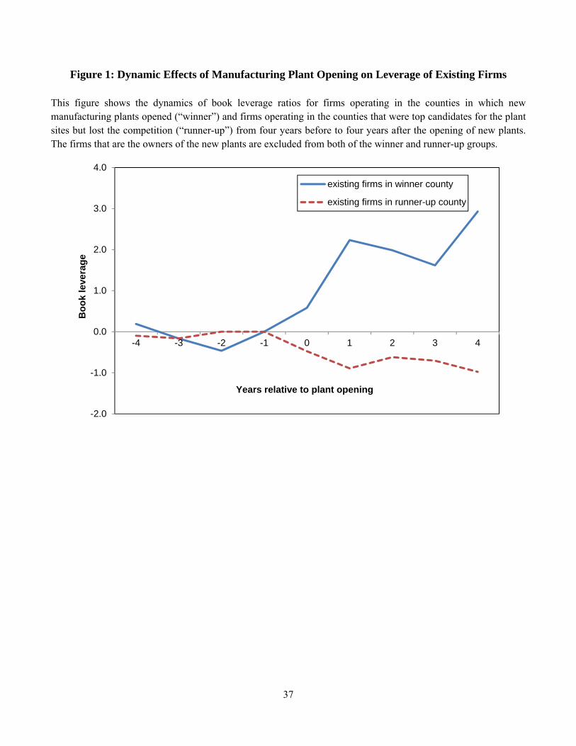
37

Figure 1: Dynamic Effects of Manufacturing Plant Opening on Leverage of Existing Firms

This figure shows the dynamics of book leverage ratios for firms operating in the counties in which new manufacturing plants opened (“winner”) and firms operating in the counties that were top candidates for the plant sites but lost the competition (“runner-up”) from four years before to four years after the opening of new plants. The firms that are the owners of the new plants are excluded from both of the winner and runner-up groups.

-2.0

-1.0

0.0

1.0

2.0

3.0

4.0

-4 -3 -2 -1 0 1 2 3 4

Bo

ok

leve

rag

e

Years relative to plant opening

existing firms in winner county

existing firms in runner-up county

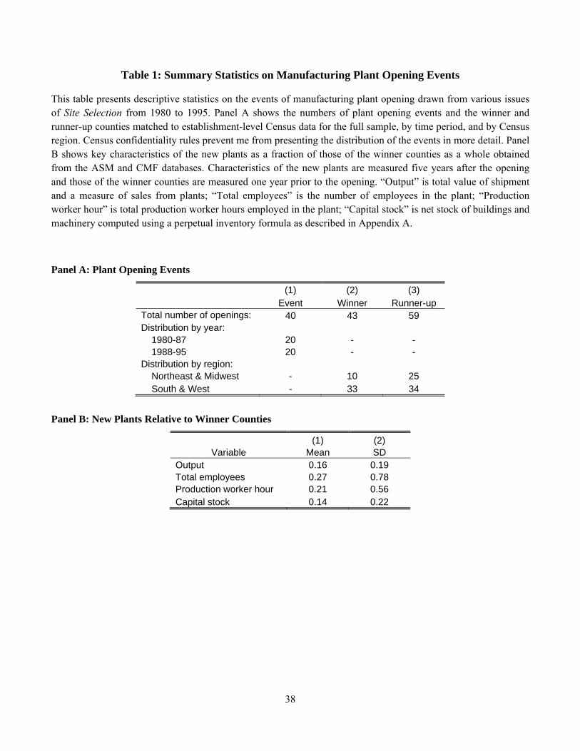
38

Table 1: Summary Statistics on Manufacturing Plant Opening Events

This table presents descriptive statistics on the events of manufacturing plant opening drawn from various issues of Site Selection from 1980 to 1995. Panel A shows the numbers of plant opening events and the winner and runner-up counties matched to establishment-level Census data for the full sample, by time period, and by Census region. Census confidentiality rules prevent me from presenting the distribution of the events in more detail. Panel B shows key characteristics of the new plants as a fraction of those of the winner counties as a whole obtained from the ASM and CMF databases. Characteristics of the new plants are measured five years after the opening and those of the winner counties are measured one year prior to the opening. “Output” is total value of shipment and a measure of sales from plants; “Total employees” is the number of employees in the plant; “Production worker hour” is total production worker hours employed in the plant; “Capital stock” is net stock of buildings and machinery computed using a perpetual inventory formula as described in Appendix A.

Panel A: Plant Opening Events

(1) (2) (3) Event Winner Runner-up Total number of openings: 40 43 59 Distribution by year: 1980-87 20 - - 1988-95 20 - - Distribution by region: Northeast & Midwest - 10 25 South & West - 33 34

Panel B: New Plants Relative to Winner Counties

(1) (2) Variable Mean SD

Output 0.16 0.19 Total employees 0.27 0.78 Production worker hour 0.21 0.56 Capital stock 0.14 0.22

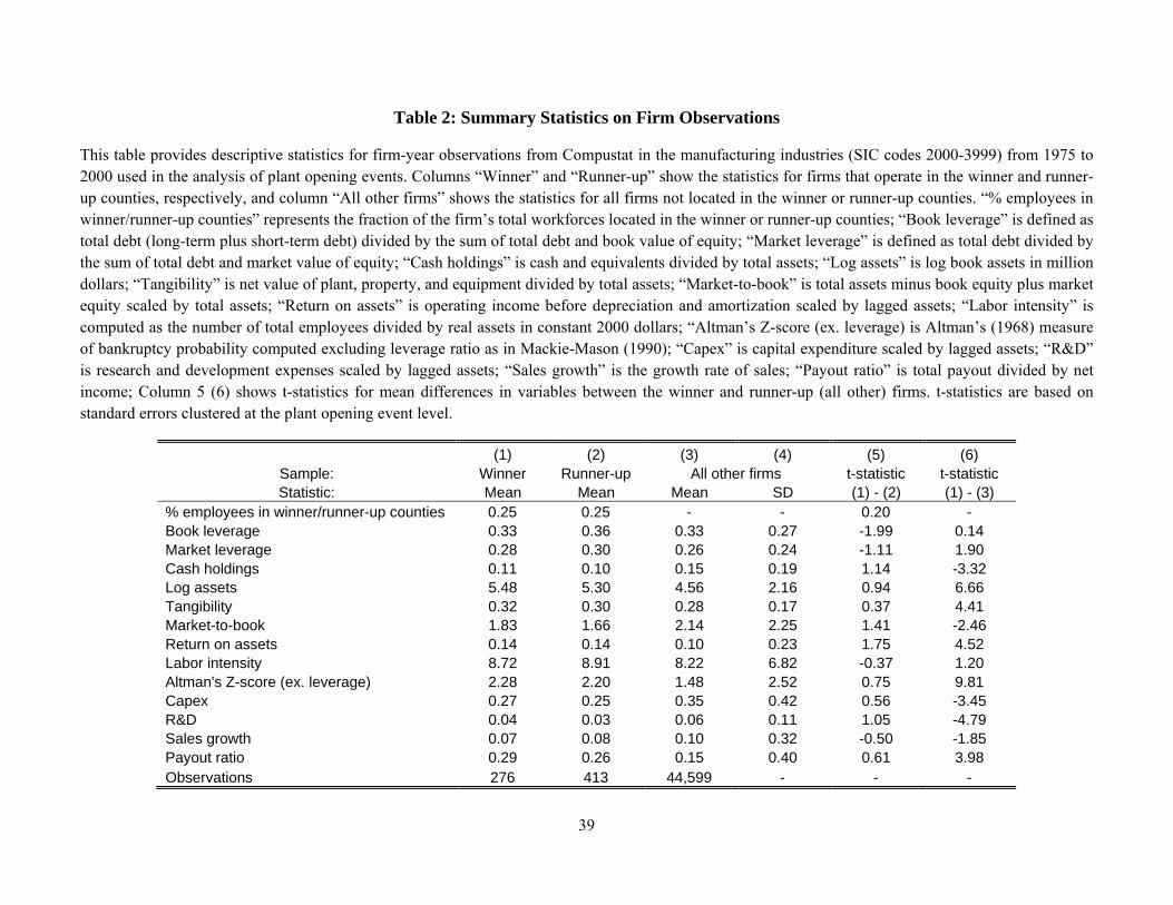
39

Table 2: Summary Statistics on Firm Observations

This table provides descriptive statistics for firm-year observations from Compustat in the manufacturing industries (SIC codes 2000-3999) from 1975 to 2000 used in the analysis of plant opening events. Columns “Winner” and “Runner-up” show the statistics for firms that operate in the winner and runner-up counties, respectively, and column “All other firms” shows the statistics for all firms not located in the winner or runner-up counties. “% employees in winner/runner-up counties” represents the fraction of the firm’s total workforces located in the winner or runner-up counties; “Book leverage” is defined as total debt (long-term plus short-term debt) divided by the sum of total debt and book value of equity; “Market leverage” is defined as total debt divided by the sum of total debt and market value of equity; “Cash holdings” is cash and equivalents divided by total assets; “Log assets” is log book assets in million dollars; “Tangibility” is net value of plant, property, and equipment divided by total assets; “Market-to-book” is total assets minus book equity plus market equity scaled by total assets; “Return on assets” is operating income before depreciation and amortization scaled by lagged assets; “Labor intensity” is computed as the number of total employees divided by real assets in constant 2000 dollars; “Altman’s Z-score (ex. leverage) is Altman’s (1968) measure of bankruptcy probability computed excluding leverage ratio as in Mackie-Mason (1990); “Capex” is capital expenditure scaled by lagged assets; “R&D” is research and development expenses scaled by lagged assets; “Sales growth” is the growth rate of sales; “Payout ratio” is total payout divided by net income; Column 5 (6) shows t-statistics for mean differences in variables between the winner and runner-up (all other) firms. t-statistics are based on standard errors clustered at the plant opening event level.

(1) (2) (3) (4) (5) (6) Sample: Winner Runner-up All other firms t-statistic t-statistic Statistic: Mean Mean Mean SD (1) - (2) (1) - (3)

% employees in winner/runner-up counties 0.25 0.25 - - 0.20 - Book leverage 0.33 0.36 0.33 0.27 -1.99 0.14 Market leverage 0.28 0.30 0.26 0.24 -1.11 1.90 Cash holdings 0.11 0.10 0.15 0.19 1.14 -3.32 Log assets 5.48 5.30 4.56 2.16 0.94 6.66 Tangibility 0.32 0.30 0.28 0.17 0.37 4.41 Market-to-book 1.83 1.66 2.14 2.25 1.41 -2.46 Return on assets 0.14 0.14 0.10 0.23 1.75 4.52 Labor intensity 8.72 8.91 8.22 6.82 -0.37 1.20 Altman's Z-score (ex. leverage) 2.28 2.20 1.48 2.52 0.75 9.81 Capex 0.27 0.25 0.35 0.42 0.56 -3.45 R&D 0.04 0.03 0.06 0.11 1.05 -4.79 Sales growth 0.07 0.08 0.10 0.32 -0.50 -1.85 Payout ratio 0.29 0.26 0.15 0.40 0.61 3.98 Observations 276 413 44,599 - - -

40

Table 3: Effect of New Manufacturing Plants on Leverage of Existing Manufacturing Firms

This table shows the effect of the opening of a manufacturing plant on the leverage of existing manufacturing firms (Compustat SIC codes 2000-3999) that operate (i.e., have plant(s) and at least 3% of employees) in the winner county compared to those in the runner-up county for the 1975 to 2000 period. The firms that are the owners of the new plants are excluded from both of the winner and runner-up groups. Panel A shows the baseline estimates and Panel B estimates the effect conditional on the fraction of the existing firm’s employees located in the winner or runner-up counties. “Winner” and “Runner-up” are dummy variables equal to one if the firm operates in the winner and runner-up counties, respectively, and zero otherwise. “After” is a dummy variable equal to one if the firm operates in the winner or runner-up counties after the opening of a manufacturing plant, and zero otherwise. Other control variables are defined in Table 2. In Panel B, “High” (“Low”) is a dummy variable equal to one if the fraction of employees in the affected (i.e., winner or runner-up) counties is larger than (smaller than or equal to) the median. All regressions include firm, year, and plant opening event fixed effects, except for column (1) of Panel A in which the event fixed effects are excluded. In column 3 of Panel A, (two-digit SIC) industry-by-year fixed effects are included. t-statistics based on standard errors adjusted for sample clustering at the firm level are reported below coefficient estimates in parentheses.

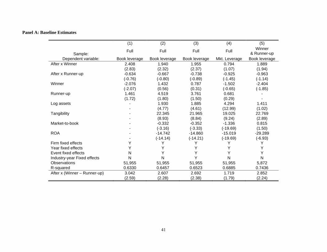
41

Panel A: Baseline Estimates

(1) (2) (3) (4) (5)

Sample: Full Full Full Full

Winner & Runner-up

Dependent variable: Book leverage Book leverage Book leverage Mkt. Leverage Book leverage After x Winner 2.408 1.940 1.955 0.794 1.889

(2.83) (2.32) (2.37) (1.07) (1.94) After x Runner-up -0.634 -0.667 -0.738 -0.925 -0.963

(-0.76) (-0.80) (-0.89) (-1.45) (-1.14) Winner -2.076 1.432 0.787 -1.502 -2.404

(-2.07) (0.56) (0.31) (-0.65) (-1.85) Runner-up 1.461 4.519 3.761 0.681 -

(1.72) (1.80) (1.50) (0.29) - Log assets - 1.930 1.885 4.294 1.411

- (4.77) (4.61) (12.99) (1.02) Tangibility - 22.345 21.965 19.025 22.769

- (8.93) (8.84) (9.24) (2.89) Market-to-book - -0.332 -0.352 -1.336 0.815

- (-3.16) (-3.33) (-19.69) (1.50) ROA - -14.742 -14.860 -15.019 -29.289

- (-14.14) (-14.21) (-19.69) (-6.93) Firm fixed effects Y Y Y Y Y Year fixed effects Y Y Y Y Y Event fixed effects N Y Y Y Y Industry-year Fixed effects N N Y N N Observations 51,955 51,955 51,955 51,955 5,872 R-squared 0.6330 0.6457 0.6523 0.6885 0.7436 After x (Winner – Runner-up) 3.042 2.607 2.692 1.719 2.852 (2.59) (2.28) (2.38) (1.79) (2.24)

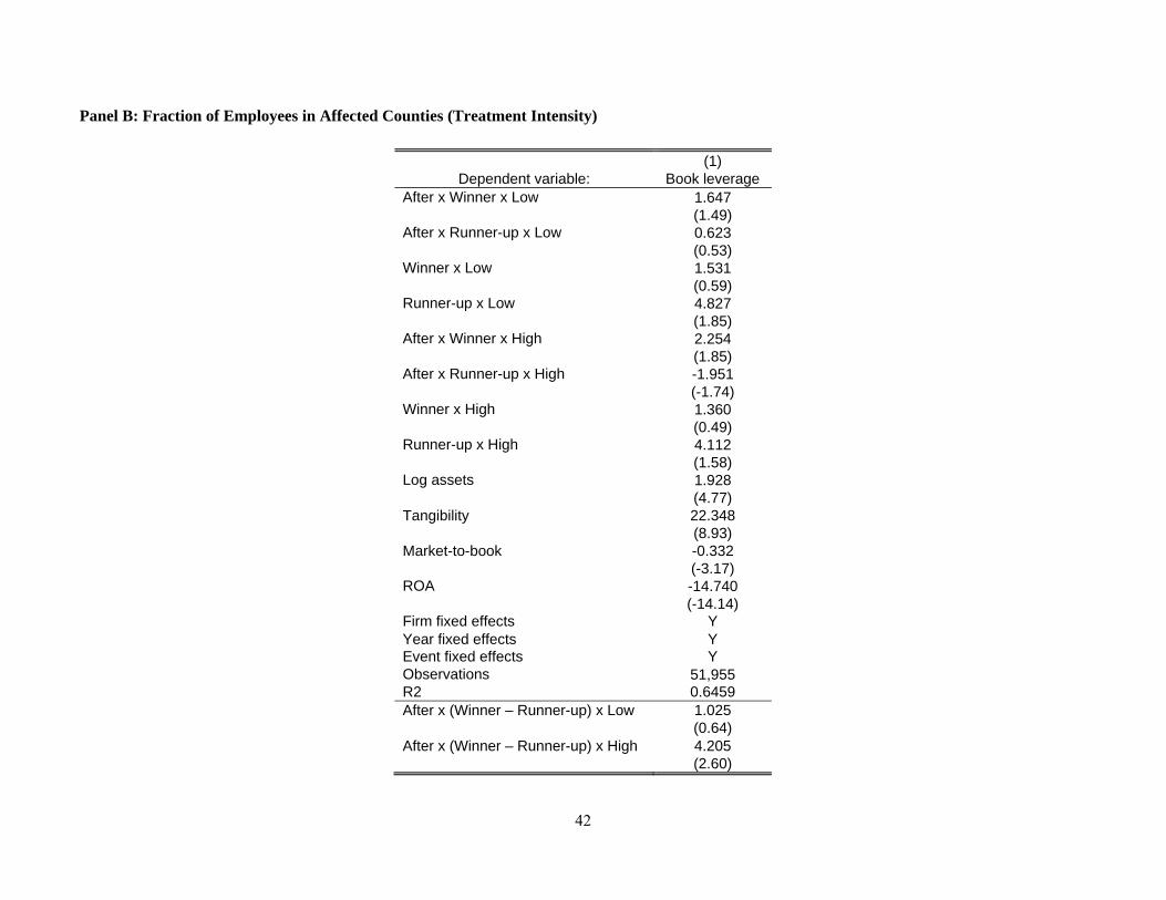
42

Panel B: Fraction of Employees in Affected Counties (Treatment Intensity)

(1) Dependent variable: Book leverage

After x Winner x Low 1.647 (1.49)

After x Runner-up x Low 0.623 (0.53)

Winner x Low 1.531 (0.59)

Runner-up x Low 4.827 (1.85)

After x Winner x High 2.254 (1.85)

After x Runner-up x High -1.951 (-1.74)

Winner x High 1.360 (0.49)

Runner-up x High 4.112 (1.58)

Log assets 1.928 (4.77)

Tangibility 22.348 (8.93)

Market-to-book -0.332 (-3.17)

ROA -14.740 (-14.14)

Firm fixed effects Y Year fixed effects Y Event fixed effects Y Observations 51,955 R2 0.6459 After x (Winner – Runner-up) x Low 1.025

(0.64) After x (Winner – Runner-up) x High 4.205 (2.60)

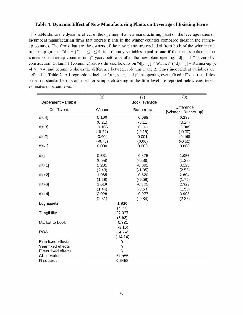
43

Table 4: Dynamic Effect of New Manufacturing Plants on Leverage of Existing Firms

This table shows the dynamic effect of the opening of a new manufacturing plant on the leverage ratios of incumbent manufacturing firms that operate plants in the winner counties compared those in the runner-up counties. The firms that are the owners of the new plants are excluded from both of the winner and runner-up groups. “d[t + j]”, -4 ≤ j ≤ 4, is a dummy variables equal to one if the firm is either in the winner or runner-up counties in “j” years before or after the new plant opening. “d[t – 1]” is zero by construction. Column 1 (column 2) shows the coefficients on “d[t + j] × Winner” (“d[t + j] × Runner-up”), -4 ≤ j ≤ 4, and column 3 shows the difference between columns 1 and 2. Other independent variables are defined in Table 2. All regressions include firm, year, and plant opening event fixed effects. t-statistics based on standard errors adjusted for sample clustering at the firm level are reported below coefficient estimates in parentheses.

(1) (2) (3) Dependent Variable: Book leverage

Coefficient: Winner Runner-up Difference

[Winner - Runner-up] d[t-4] 0.190 -0.098 0.287

(0.21) (-0.11) (0.24) d[t-3] -0.166 -0.161 -0.005

(-0.22) (-0.19) (-0.00) d[t-2] -0.464 0.001 -0.465

(-0.76) (0.00) (-0.52) d[t-1] 0.000 0.000 0.000

- - - d[t] 0.581 -0.475 1.056

(0.98) (-0.80) (1.28) d[t+1] 2.231 -0.892 3.123

(2.43) (-1.05) (2.55) d[t+2] 1.985 -0.620 2.604

(1.89) (-0.56) (1.75) d[t+3] 1.618 -0.705 2.323

(1.46) (-0.63) (1.50) d[t+4] 2.928 -0.977 3.905

(2.31) (-0.84) (2.35) Log assets 1.930

(4.77) Tangibility 22.337

(8.93) Market-to-book -0.331

(-3.15) ROA -14.745

(-14.14) Firm fixed effects Y Year fixed effects Y Event fixed effects Y Observations 51,955 R-squared 0.6458

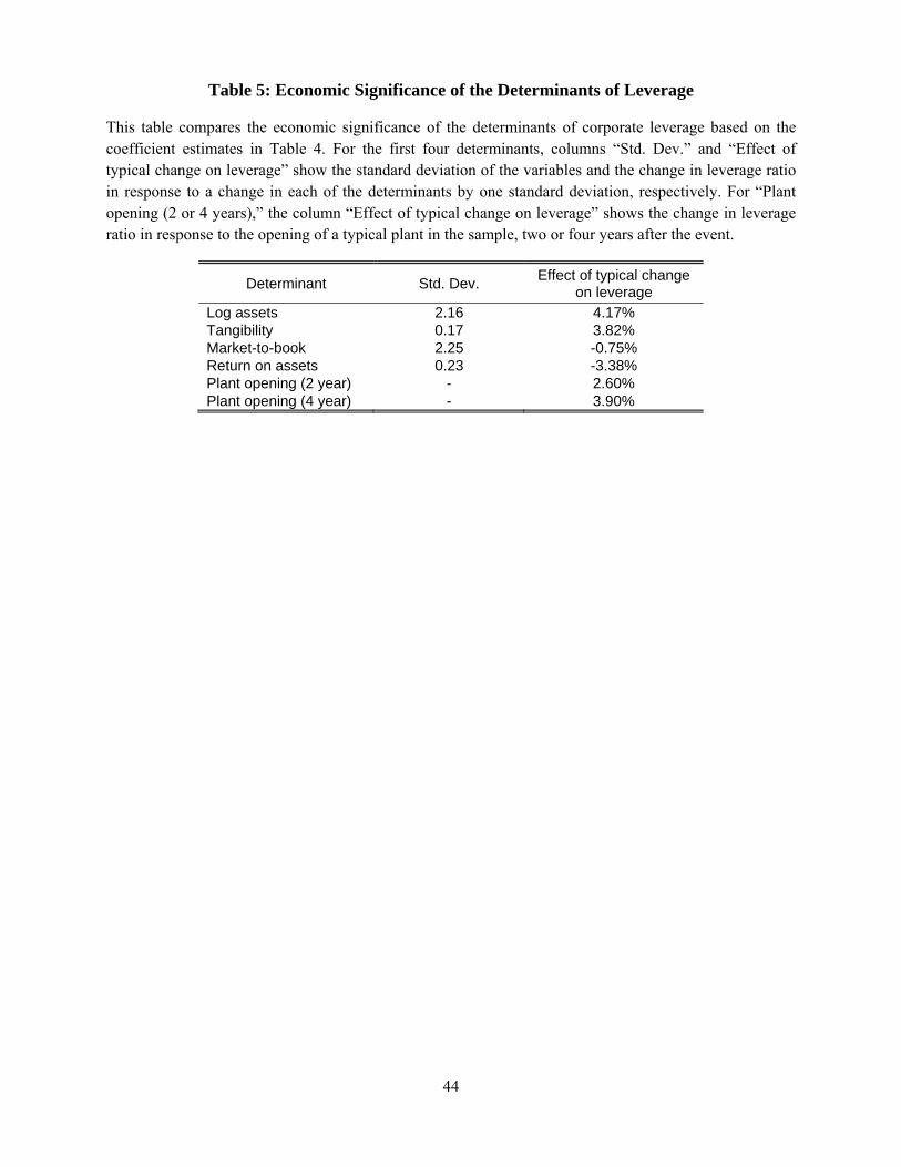
44

Table 5: Economic Significance of the Determinants of Leverage

This table compares the economic significance of the determinants of corporate leverage based on the coefficient estimates in Table 4. For the first four determinants, columns “Std. Dev.” and “Effect of typical change on leverage” show the standard deviation of the variables and the change in leverage ratio in response to a change in each of the determinants by one standard deviation, respectively. For “Plant opening (2 or 4 years),” the column “Effect of typical change on leverage” shows the change in leverage ratio in response to the opening of a typical plant in the sample, two or four years after the event.

Determinant Std. Dev. Effect of typical change

on leverage Log assets 2.16 4.17% Tangibility 0.17 3.82% Market-to-book 2.25 -0.75% Return on assets 0.23 -3.38% Plant opening (2 year) - 2.60% Plant opening (4 year) - 3.90%

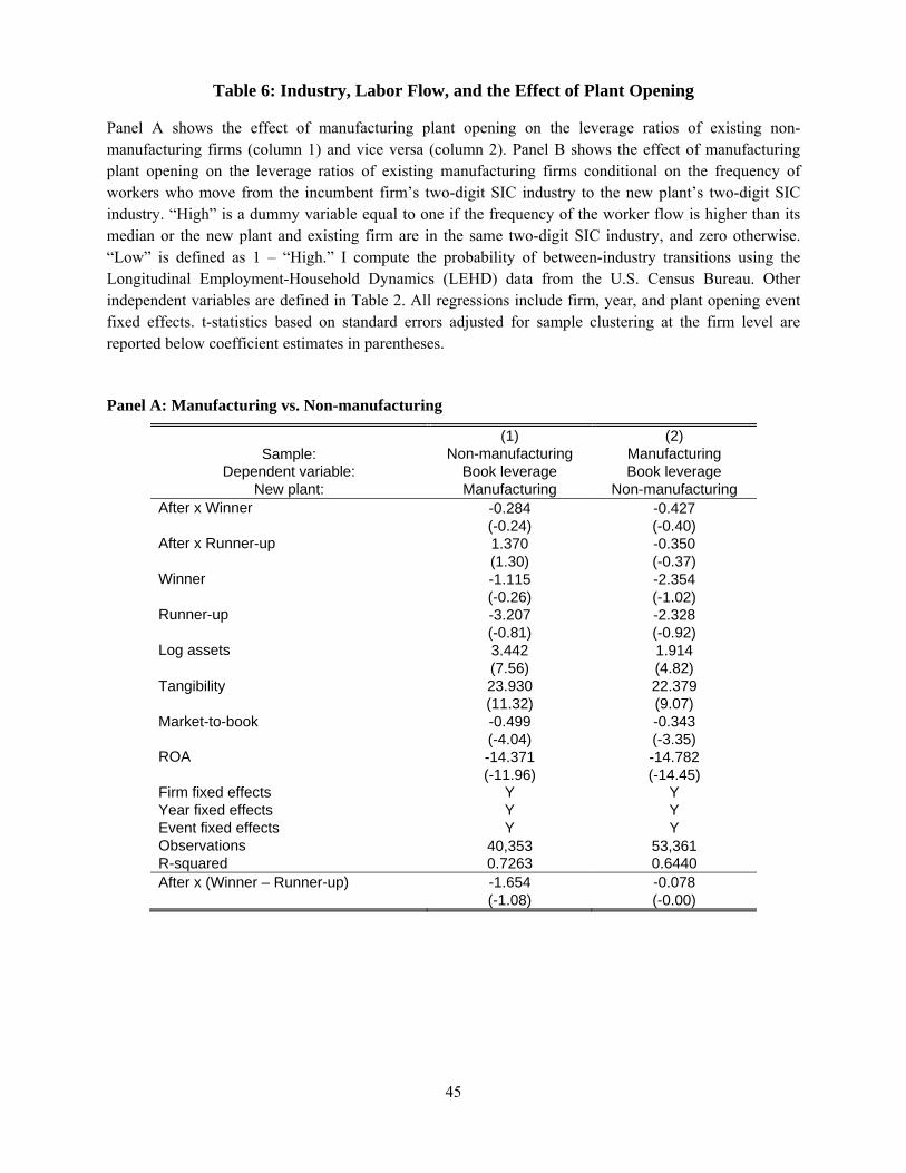
45

Table 6: Industry, Labor Flow, and the Effect of Plant Opening

Panel A shows the effect of manufacturing plant opening on the leverage ratios of existing non-manufacturing firms (column 1) and vice versa (column 2). Panel B shows the effect of manufacturing plant opening on the leverage ratios of existing manufacturing firms conditional on the frequency of workers who move from the incumbent firm’s two-digit SIC industry to the new plant’s two-digit SIC industry. “High” is a dummy variable equal to one if the frequency of the worker flow is higher than its median or the new plant and existing firm are in the same two-digit SIC industry, and zero otherwise. “Low” is defined as 1 – “High.” I compute the probability of between-industry transitions using the Longitudinal Employment-Household Dynamics (LEHD) data from the U.S. Census Bureau. Other independent variables are defined in Table 2. All regressions include firm, year, and plant opening event fixed effects. t-statistics based on standard errors adjusted for sample clustering at the firm level are reported below coefficient estimates in parentheses.

Panel A: Manufacturing vs. Non-manufacturing

(1) (2) Sample: Non-manufacturing Manufacturing

Dependent variable: Book leverage Book leverage New plant: Manufacturing Non-manufacturing

After x Winner -0.284 -0.427 (-0.24) (-0.40)

After x Runner-up 1.370 -0.350 (1.30) (-0.37)

Winner -1.115 -2.354 (-0.26) (-1.02)

Runner-up -3.207 -2.328 (-0.81) (-0.92)

Log assets 3.442 1.914 (7.56) (4.82)

Tangibility 23.930 22.379 (11.32) (9.07)

Market-to-book -0.499 -0.343 (-4.04) (-3.35)

ROA -14.371 -14.782 (-11.96) (-14.45)

Firm fixed effects Y Y Year fixed effects Y Y Event fixed effects Y Y Observations 40,353 53,361 R-squared 0.7263 0.6440 After x (Winner – Runner-up) -1.654 -0.078 (-1.08) (-0.00)

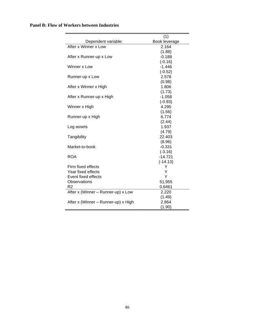
46

Panel B: Flow of Workers between Industries

(1) Dependent variable: Book leverage

After x Winner x Low 2.164 (1.88)

After x Runner-up x Low -0.188 (-0.16)

Winner x Low -1.446 (-0.52)

Runner-up x Low 2.578 (0.98)

After x Winner x High 1.806 (1.73)

After x Runner-up x High -1.058 (-0.93)

Winner x High 4.295 (1.56)

Runner-up x High 6.774 (2.44)

Log assets 1.937 (4.79)

Tangibility 22.403 (8.96)

Market-to-book -0.331 (-3.16)

ROA -14.721 (-14.13)

Firm fixed effects Y Year fixed effects Y Event fixed effects Y Observations 51,955 R2 0.6461 After x (Winner – Runner-up) x Low 2.220

(1.49) After x (Winner – Runner-up) x High 2.864 (1.90)

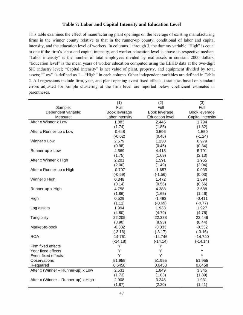
47

Table 7: Labor and Capital Intensity and Education Level

This table examines the effect of manufacturing plant openings on the leverage of existing manufacturing firms in the winner county relative to that in the runner-up county, conditional of labor and capital intensity, and the education level of workers. In columns 1 through 3, the dummy variable “High” is equal to one if the firm’s labor and capital intensity, and worker education level is above its respective median. “Labor intensity” is the number of total employees divided by real assets in constant 2000 dollars; “Education level” is the mean years of worker education computed using the LEHD data at the two-digit SIC industry level; “Capital intensity” is net value of plant, property, and equipment divided by total assets; “Low” is defined as 1 – “High” in each column. Other independent variables are defined in Table 2. All regressions include firm, year, and plant opening event fixed effects. t-statistics based on standard errors adjusted for sample clustering at the firm level are reported below coefficient estimates in parentheses.

(1) (2) (3) Sample: Full Full Full

Dependent variable: Book leverage Book leverage Book leverage Measure: Labor intensity Education level Capital intensity

After x Winner x Low 1.883 2.445 1.794 (1.74) (1.85) (1.32)

After x Runner-up x Low -0.648 0.596 -1.550 (-0.62) (0.46) (-1.24)

Winner x Low 2.579 1.230 0.979 (0.98) (0.45) (0.34)

Runner-up x Low 4.569 4.418 5.791 (1.75) (1.69) (2.13)

After x Winner x High 2.201 1.591 1.965 (2.00) (1.49) (2.04)

After x Runner-up x High -0.707 -1.657 0.035 (-0.59) (-1.56) (0.03)

Winner x High 0.348 1.472 1.694 (0.14) (0.56) (0.66)

Runner-up x High 4.758 4.388 3.688 (1.86) (1.65) (1.46)

High 0.529 -1.493 -0.411 (1.11) (-0.69) (-0.77)

Log assets 1.994 1.933 1.927 (4.80) (4.79) (4.76)

Tangibility 22.205 22.338 23.446 (8.90) (8.93) (8.44)

Market-to-book -0.332 -0.333 -0.332 (-3.16) (-3.17) (-3.16)

ROA -14.761 -14.746 -14.740 (-14.18) (-14.14) (-14.14)

Firm fixed effects Y Y Y Year fixed effects Y Y Y Event fixed effects Y Y Y Observations 51,955 51,955 51,955 R-squared 0.6458 0.6458 0.6458 After x (Winner – Runner-up) x Low 2.531 1.849 3.345

(1.73) (1.03) (1.89) After x (Winner – Runner-up) x High 2.908 3.248 1.931 (1.87) (2.20) (1.41)

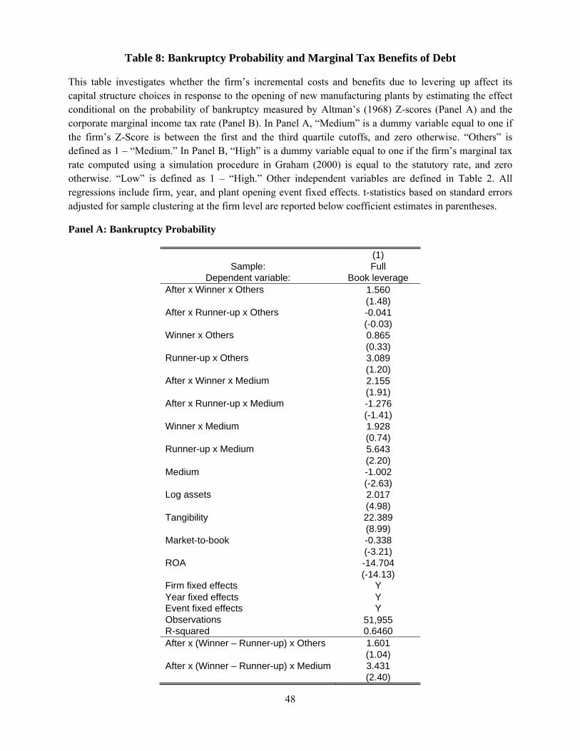
48

Table 8: Bankruptcy Probability and Marginal Tax Benefits of Debt

This table investigates whether the firm’s incremental costs and benefits due to levering up affect its capital structure choices in response to the opening of new manufacturing plants by estimating the effect conditional on the probability of bankruptcy measured by Altman’s (1968) Z-scores (Panel A) and the corporate marginal income tax rate (Panel B). In Panel A, “Medium” is a dummy variable equal to one if the firm’s Z-Score is between the first and the third quartile cutoffs, and zero otherwise. “Others” is defined as 1 – “Medium.” In Panel B, “High” is a dummy variable equal to one if the firm’s marginal tax rate computed using a simulation procedure in Graham (2000) is equal to the statutory rate, and zero otherwise. “Low” is defined as 1 – “High.” Other independent variables are defined in Table 2. All regressions include firm, year, and plant opening event fixed effects. t-statistics based on standard errors adjusted for sample clustering at the firm level are reported below coefficient estimates in parentheses.

Panel A: Bankruptcy Probability

(1) Sample: Full

Dependent variable: Book leverage After x Winner x Others 1.560

(1.48) After x Runner-up x Others -0.041

(-0.03) Winner x Others 0.865

(0.33) Runner-up x Others 3.089

(1.20) After x Winner x Medium 2.155

(1.91) After x Runner-up x Medium -1.276

(-1.41) Winner x Medium 1.928

(0.74) Runner-up x Medium 5.643

(2.20) Medium -1.002

(-2.63) Log assets 2.017

(4.98) Tangibility 22.389

(8.99) Market-to-book -0.338

(-3.21) ROA -14.704

(-14.13) Firm fixed effects Y Year fixed effects Y Event fixed effects Y Observations 51,955 R-squared 0.6460 After x (Winner – Runner-up) x Others 1.601

(1.04) After x (Winner – Runner-up) x Medium 3.431 (2.40)

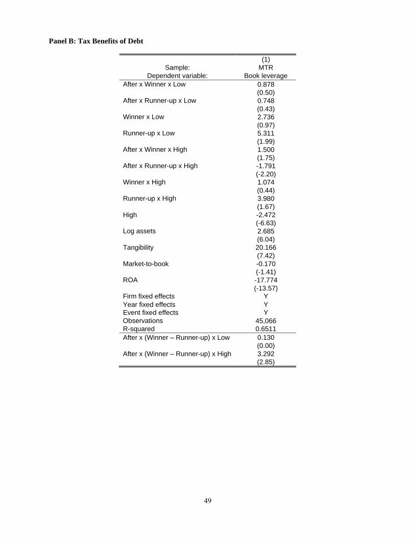
49

Panel B: Tax Benefits of Debt

(1) Sample: MTR

Dependent variable: Book leverage After x Winner x Low 0.878

(0.50) After x Runner-up x Low 0.748

(0.43) Winner x Low 2.736

(0.97) Runner-up x Low 5.311

(1.99) After x Winner x High 1.500

(1.75) After x Runner-up x High -1.791

(-2.20) Winner x High 1.074

(0.44) Runner-up x High 3.980

(1.67) High -2.472

(-6.63) Log assets 2.685

(6.04) Tangibility 20.166

(7.42) Market-to-book -0.170

(-1.41) ROA -17.774

(-13.57) Firm fixed effects Y Year fixed effects Y Event fixed effects Y Observations 45,066 R-squared 0.6511 After x (Winner – Runner-up) x Low 0.130

(0.00) After x (Winner – Runner-up) x High 3.292 (2.85)

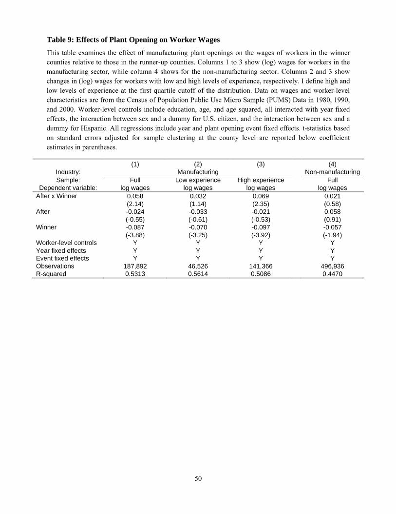
50

Table 9: Effects of Plant Opening on Worker Wages

This table examines the effect of manufacturing plant openings on the wages of workers in the winner counties relative to those in the runner-up counties. Columns 1 to 3 show (log) wages for workers in the manufacturing sector, while column 4 shows for the non-manufacturing sector. Columns 2 and 3 show changes in (log) wages for workers with low and high levels of experience, respectively. I define high and low levels of experience at the first quartile cutoff of the distribution. Data on wages and worker-level characteristics are from the Census of Population Public Use Micro Sample (PUMS) Data in 1980, 1990, and 2000. Worker-level controls include education, age, and age squared, all interacted with year fixed effects, the interaction between sex and a dummy for U.S. citizen, and the interaction between sex and a dummy for Hispanic. All regressions include year and plant opening event fixed effects. t-statistics based on standard errors adjusted for sample clustering at the county level are reported below coefficient estimates in parentheses.

(1) (2) (3) (4) Industry: Manufacturing Non-manufacturing Sample: Full Low experience High experience Full

Dependent variable: log wages log wages log wages log wages After x Winner 0.058 0.032 0.069 0.021

(2.14) (1.14) (2.35) (0.58) After -0.024 -0.033 -0.021 0.058

(-0.55) (-0.61) (-0.53) (0.91) Winner -0.087 -0.070 -0.097 -0.057

(-3.88) (-3.25) (-3.92) (-1.94) Worker-level controls Y Y Y Y Year fixed effects Y Y Y Y Event fixed effects Y Y Y Y Observations 187,892 46,526 141,366 496,936 R-squared 0.5313 0.5614 0.5086 0.4470

51

Table 10: Alternative Explanations and Robustness

This table examines the robustness of the main results to alternative explanations concerning agglomeration spillovers (Panel A), local product market competition (Panel B), and the non-even distribution of the winner and runner-up counties among geographic regions (Panel C). Panel A includes additional control variables to capture the effect of potential agglomeration spillovers on total factor productivity (TFP) and property values. “TFP” is estimated as the residual of the year by three-digit SIC industry production function regression of log real output on log labor hours, log real capital stock, and log materials following a method in Lichtenberg (1992). I assume production functions take the Cobb-Douglas or translog functional form. The computed plant-level TFP is aggregated at the firm level using real capital stock as weight. “Property values” are hand-collected from the Survey of Government, Volume 2 Taxable Property Values and Assessment-Sales Price Ratios (1977, 1982, 1987, and 1992). Panel B shows the effect of plant openings on leverage conditional on the product market competition of the winner counties measured one year prior to the opening. In column 1 (column 2), “High” is a dummy variable equal to one if the Herfindahl-Hirschman Index (HHI) computed at the all manufacturing industries and county (two-digit SIC industry and county) level is larger than the median, and zero otherwise. Panel C estimates the effect of manufacturing plant opening focusing on events in which both of the winner and runner-up counties are in the same Census region (i.e., Northeast, Midwest, South, or West). Other independent variables are defined in Table 2. All regressions include firm, year, and plant opening event fixed effects. t-statistics based on standard errors adjusted for sample clustering at the firm level are reported below coefficient estimates in parentheses.

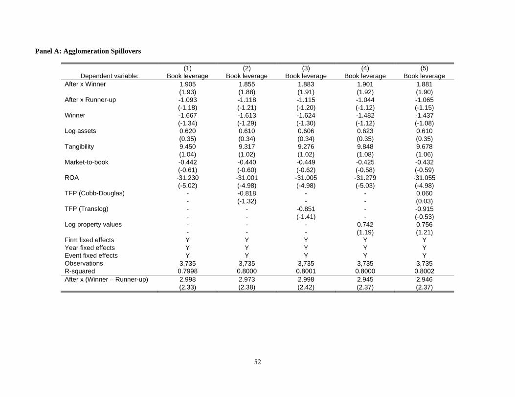
52

Panel A: Agglomeration Spillovers

(1) (2) (3) (4) (5) Dependent variable: Book leverage Book leverage Book leverage Book leverage Book leverage

After x Winner 1.905 1.855 1.883 1.901 1.881 (1.93) (1.88) (1.91) (1.92) (1.90)

After x Runner-up -1.093 -1.118 -1.115 -1.044 -1.065 (-1.18) (-1.21) (-1.20) (-1.12) (-1.15)

Winner -1.667 -1.613 -1.624 -1.482 -1.437 (-1.34) (-1.29) (-1.30) (-1.12) (-1.08)

Log assets 0.620 0.610 0.606 0.623 0.610 (0.35) (0.34) (0.34) (0.35) (0.35)

Tangibility 9.450 9.317 9.276 9.848 9.678 (1.04) (1.02) (1.02) (1.08) (1.06)

Market-to-book -0.442 -0.440 -0.449 -0.425 -0.432 (-0.61) (-0.60) (-0.62) (-0.58) (-0.59)

ROA -31.230 -31.001 -31.005 -31.279 -31.055 (-5.02) (-4.98) (-4.98) (-5.03) (-4.98)

TFP (Cobb-Douglas) - -0.818 - - 0.060 - (-1.32) - - (0.03)

TFP (Translog) - - -0.851 - -0.915 - - (-1.41) - (-0.53)

Log property values - - - 0.742 0.756 - - - (1.19) (1.21)

Firm fixed effects Y Y Y Y Y Year fixed effects Y Y Y Y Y Event fixed effects Y Y Y Y Y Observations 3,735 3,735 3,735 3,735 3,735 R-squared 0.7998 0.8000 0.8001 0.8000 0.8002 After x (Winner – Runner-up) 2.998 2.973 2.998 2.945 2.946 (2.33) (2.38) (2.42) (2.37) (2.37)

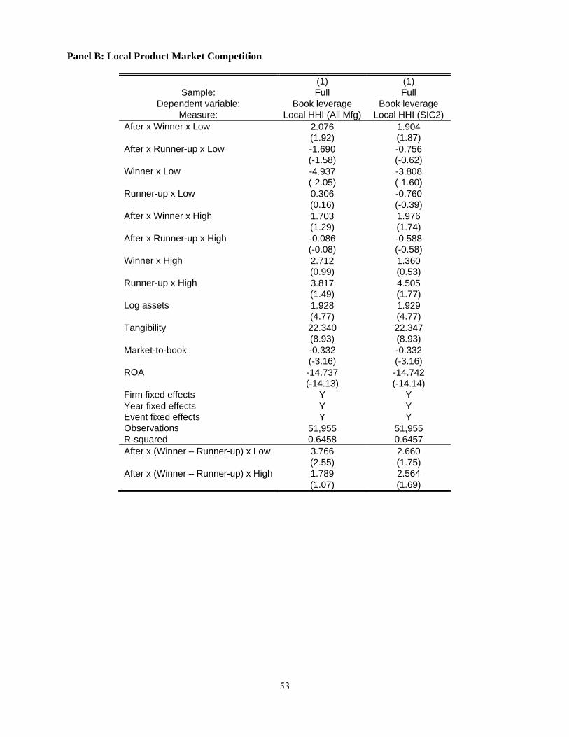
53

Panel B: Local Product Market Competition

(1) (1) Sample: Full Full

Dependent variable: Book leverage Book leverage Measure: Local HHI (All Mfg) Local HHI (SIC2)

After x Winner x Low 2.076 1.904 (1.92) (1.87)

After x Runner-up x Low -1.690 -0.756 (-1.58) (-0.62)

Winner x Low -4.937 -3.808 (-2.05) (-1.60)

Runner-up x Low 0.306 -0.760 (0.16) (-0.39)

After x Winner x High 1.703 1.976 (1.29) (1.74)

After x Runner-up x High -0.086 -0.588 (-0.08) (-0.58)

Winner x High 2.712 1.360 (0.99) (0.53)

Runner-up x High 3.817 4.505 (1.49) (1.77)

Log assets 1.928 1.929 (4.77) (4.77)

Tangibility 22.340 22.347 (8.93) (8.93)

Market-to-book -0.332 -0.332 (-3.16) (-3.16)

ROA -14.737 -14.742 (-14.13) (-14.14)

Firm fixed effects Y Y Year fixed effects Y Y Event fixed effects Y Y Observations 51,955 51,955 R-squared 0.6458 0.6457 After x (Winner – Runner-up) x Low 3.766 2.660

(2.55) (1.75) After x (Winner – Runner-up) x High 1.789 2.564 (1.07) (1.69)

54

Panel C: Non-even Distribution of Winners and Runner-ups among Geographical Regions

(1) Dependent variable: Book leverage

After x Winner x Others 2.034 (1.78)

After x Runner-up x Others -0.566 (-0.60)

Winner x Others 1.389 (0.54)

Runner-up x Others 4.463 (1.75)

After x Winner x Same region 1.851 (1.57)

After x Runner-up x Same region -0.878 (-0.65)

Winner x Same region -2.808 (-0.81)

Runner-up x Same region 0.365 (0.10)

Log assets 1.930 (4.77)

Tangibility 22.346 (8.93)

Market-to-book -0.332 (-3.16)

ROA -14.741 (-14.14)

Firm fixed effects Y Year fixed effects Y Event fixed effects Y Observations 51,955 R2 0.6457 After x (Winner – Runner-up) x Others 2.601

(1.81) After x (Winner – Runner-up) x Same 2.729

(1.54)

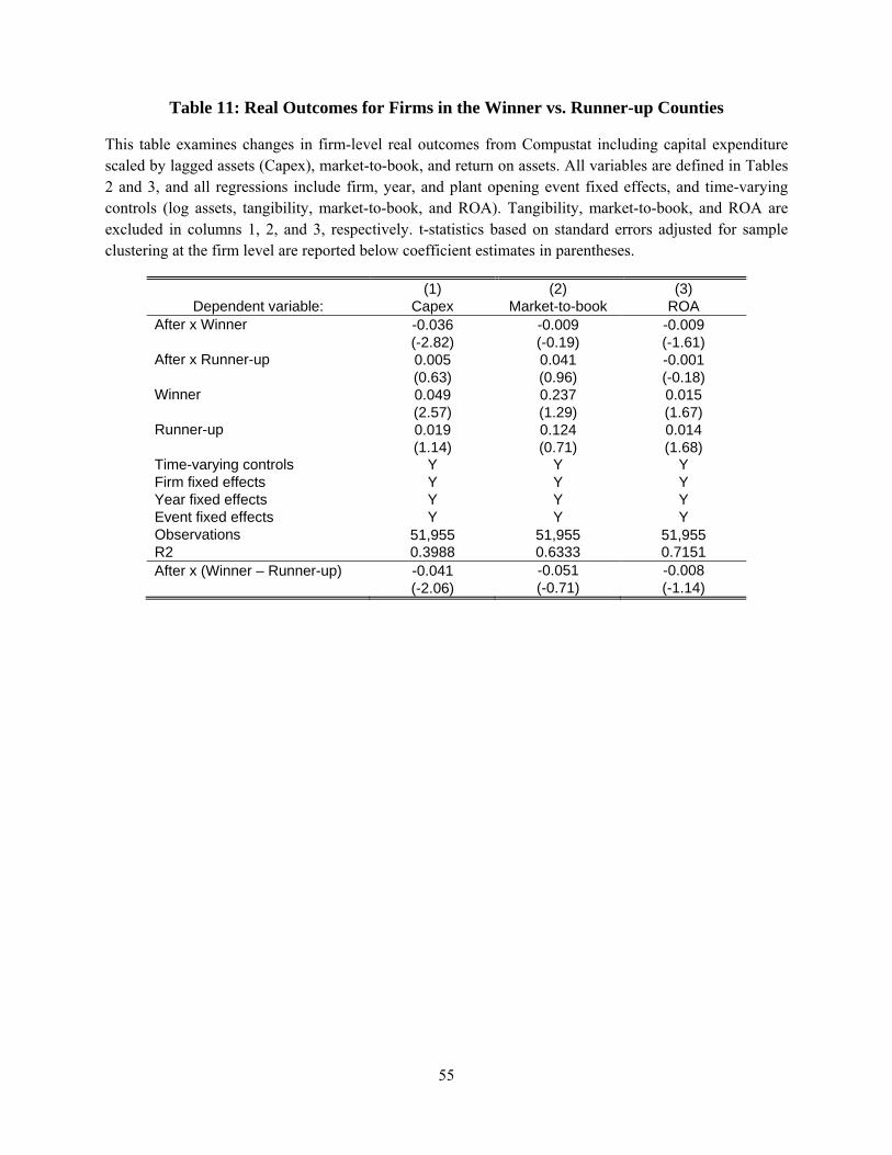
55

Table 11: Real Outcomes for Firms in the Winner vs. Runner-up Counties

This table examines changes in firm-level real outcomes from Compustat including capital expenditure scaled by lagged assets (Capex), market-to-book, and return on assets. All variables are defined in Tables 2 and 3, and all regressions include firm, year, and plant opening event fixed effects, and time-varying controls (log assets, tangibility, market-to-book, and ROA). Tangibility, market-to-book, and ROA are excluded in columns 1, 2, and 3, respectively. t-statistics based on standard errors adjusted for sample clustering at the firm level are reported below coefficient estimates in parentheses.

(1) (2) (3) Dependent variable: Capex Market-to-book ROA

After x Winner -0.036 -0.009 -0.009 (-2.82) (-0.19) (-1.61)

After x Runner-up 0.005 0.041 -0.001 (0.63) (0.96) (-0.18)

Winner 0.049 0.237 0.015 (2.57) (1.29) (1.67)

Runner-up 0.019 0.124 0.014 (1.14) (0.71) (1.68)

Time-varying controls Y Y Y Firm fixed effects Y Y Y Year fixed effects Y Y Y Event fixed effects Y Y Y Observations 51,955 51,955 51,955 R2 0.3988 0.6333 0.7151 After x (Winner – Runner-up) -0.041 -0.051 -0.008 (-2.06) (-0.71) (-1.14)

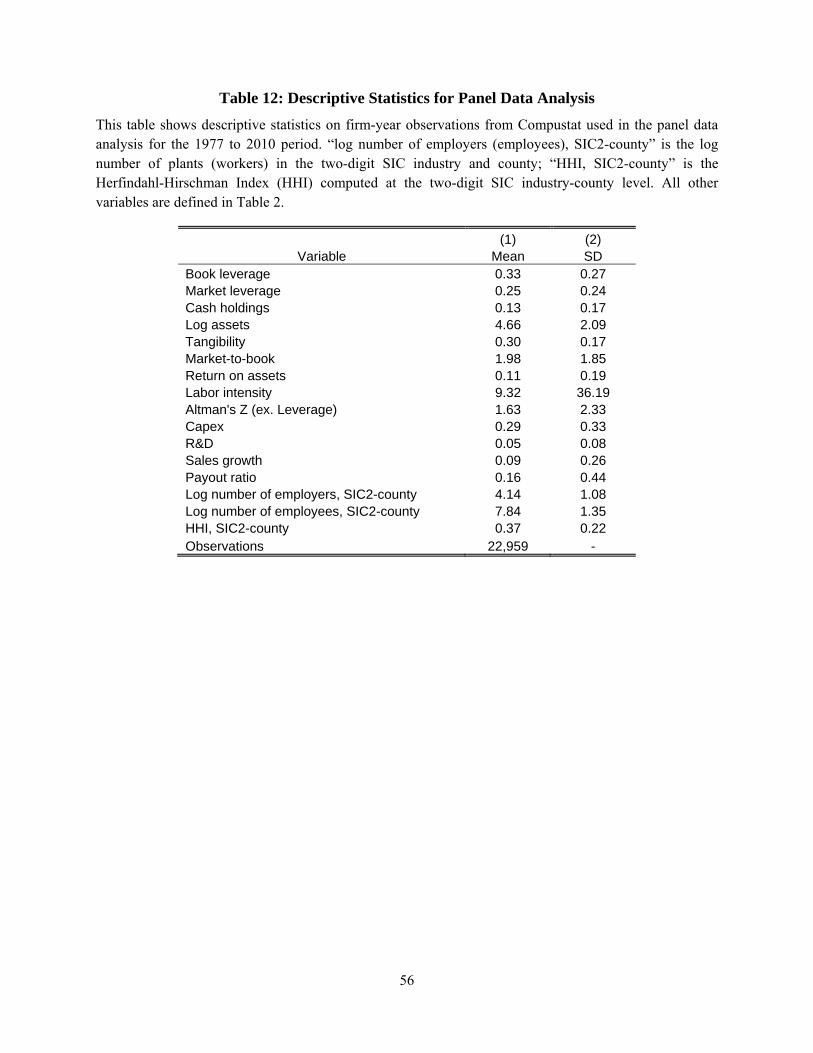
56

Table 12: Descriptive Statistics for Panel Data Analysis

This table shows descriptive statistics on firm-year observations from Compustat used in the panel data analysis for the 1977 to 2010 period. “log number of employers (employees), SIC2-county” is the log number of plants (workers) in the two-digit SIC industry and county; “HHI, SIC2-county” is the Herfindahl-Hirschman Index (HHI) computed at the two-digit SIC industry-county level. All other variables are defined in Table 2.

(1) (2) Variable Mean SD

Book leverage 0.33 0.27 Market leverage 0.25 0.24 Cash holdings 0.13 0.17 Log assets 4.66 2.09 Tangibility 0.30 0.17 Market-to-book 1.98 1.85 Return on assets 0.11 0.19 Labor intensity 9.32 36.19 Altman's Z (ex. Leverage) 1.63 2.33 Capex 0.29 0.33 R&D 0.05 0.08 Sales growth 0.09 0.26 Payout ratio 0.16 0.44 Log number of employers, SIC2-county 4.14 1.08 Log number of employees, SIC2-county 7.84 1.35 HHI, SIC2-county 0.37 0.22 Observations 22,959 -

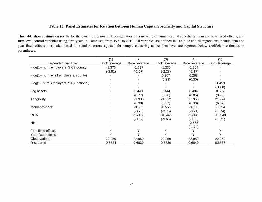
57

Table 13: Panel Estimates for Relation between Human Capital Specificity and Capital Structure

This table shows estimation results for the panel regression of leverage ratios on a measure of human capital specificity, firm and year fixed effects, and firm-level control variables using firm-years in Compustat from 1977 to 2010. All variables are defined in Table 12 and all regressions include firm and year fixed effects. t-statistics based on standard errors adjusted for sample clustering at the firm level are reported below coefficient estimates in parentheses.

(1) (2) (3) (4) (5) Dependent variable: Book leverage Book leverage Book leverage Book leverage Book leverage

- log(1+ num. employers, SIC2-county) -1.376 -1.237 -1.335 -1.264 - (-2.81) (-2.57) (-2.28) (-2.17) -

- log(1+ num. of all employers, county) - - 0.207 0.268 - - - (0.23) (0.30) -

- log(1+ num. employers, SIC2-national) - - - - -1.453 - - - - (-1.80)

Log assets - 0.440 0.444 0.484 0.567 - (0.77) (0.78) (0.85) (0.98)

Tangibility - 21.933 21.912 21.953 21.974 - (6.38) (6.37) (6.38) (6.37)

Market-to-book - -0.555 -0.555 -0.550 -0.554 - (-3.75) (-3.75) (-3.71) (-3.74)

ROA - -16.438 -16.445 -16.442 -16.548 - (-9.67) (-9.66) (-9.66) (-9.71)

HHI - - - -2.555 - - - - (-1.74) -

Firm fixed effects Y Y Y Y Y Year fixed effects Y Y Y Y Y Observations 22,959 22,959 22,959 22,959 22,959 R-squared 0.6724 0.6839 0.6839 0.6840 0.6837

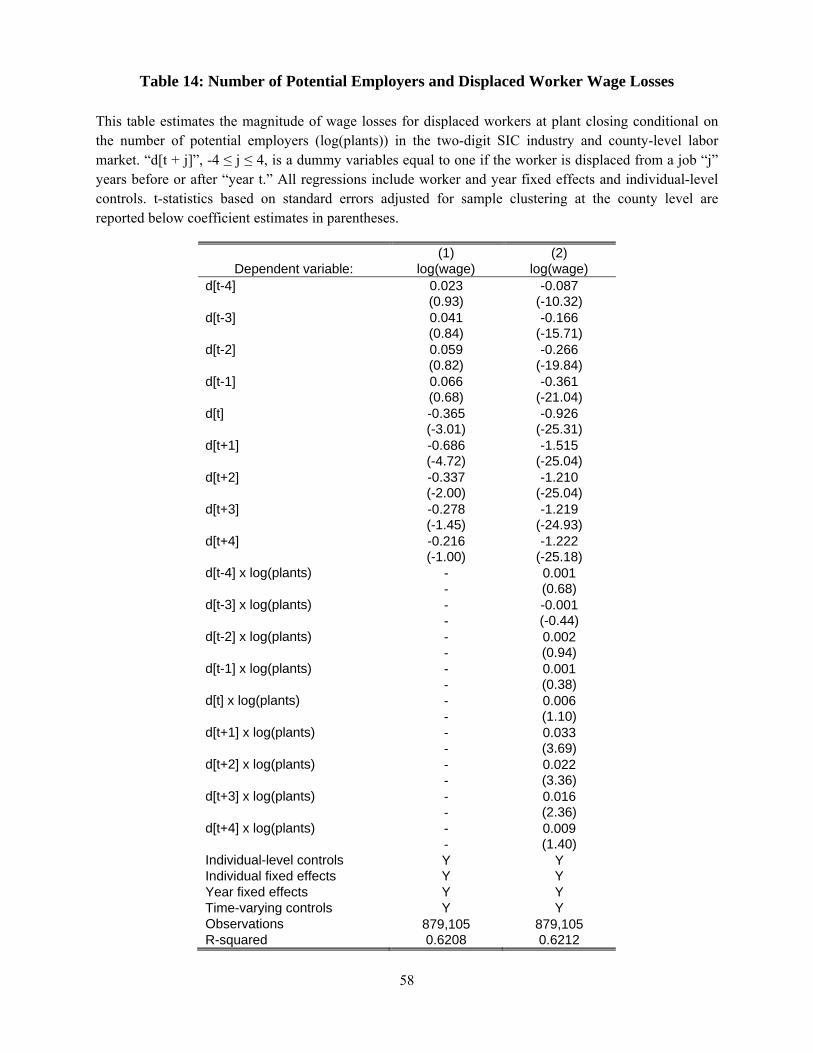
58

Table 14: Number of Potential Employers and Displaced Worker Wage Losses

This table estimates the magnitude of wage losses for displaced workers at plant closing conditional on the number of potential employers (log(plants)) in the two-digit SIC industry and county-level labor market. “d[t + j]”, -4 ≤ j ≤ 4, is a dummy variables equal to one if the worker is displaced from a job “j” years before or after “year t.” All regressions include worker and year fixed effects and individual-level controls. t-statistics based on standard errors adjusted for sample clustering at the county level are reported below coefficient estimates in parentheses.

(1) (2) Dependent variable: log(wage) log(wage)

d[t-4] 0.023 -0.087 (0.93) (-10.32)

d[t-3] 0.041 -0.166 (0.84) (-15.71)

d[t-2] 0.059 -0.266 (0.82) (-19.84)

d[t-1] 0.066 -0.361 (0.68) (-21.04)

d[t] -0.365 -0.926 (-3.01) (-25.31)

d[t+1] -0.686 -1.515 (-4.72) (-25.04)

d[t+2] -0.337 -1.210 (-2.00) (-25.04)

d[t+3] -0.278 -1.219 (-1.45) (-24.93)

d[t+4] -0.216 -1.222 (-1.00) (-25.18)

d[t-4] x log(plants) - 0.001 - (0.68)

d[t-3] x log(plants) - -0.001 - (-0.44)

d[t-2] x log(plants) - 0.002 - (0.94)

d[t-1] x log(plants) - 0.001 - (0.38)

d[t] x log(plants) - 0.006 - (1.10)

d[t+1] x log(plants) - 0.033 - (3.69)

d[t+2] x log(plants) - 0.022 - (3.36)

d[t+3] x log(plants) - 0.016 - (2.36)

d[t+4] x log(plants) - 0.009 - (1.40)

Individual-level controls Y Y Individual fixed effects Y Y Year fixed effects Y Y Time-varying controls Y Y Observations 879,105 879,105 R-squared 0.6208 0.6212

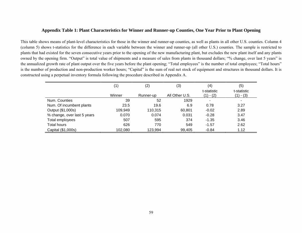
59

Appendix Table 1: Plant Characteristics for Winner and Runner-up Counties, One Year Prior to Plant Opening

This table shows means of plant-level characteristics for those in the winner and runner-up counties, as well as plants in all other U.S. counties. Column 4 (column 5) shows t-statistics for the difference in each variable between the winner and runner-up (all other U.S.) counties. The sample is restricted to plants that had existed for the seven consecutive years prior to the opening of the new manufacturing plant, but excludes the new plant itself and any plants owned by the opening firm. “Output” is total value of shipments and a measure of sales from plants in thousand dollars; “% change, over last 5 years” is the annualized growth rate of plant output over the five years before the plant opening; “Total employees” is the number of total employees; “Total hours” is the number of production and non-production worker hours; “Capital” is the sum of real net stock of equipment and structures in thousand dollars. It is constructed using a perpetual inventory formula following the procedure described in Appendix A.

(1) (2) (3) (4) (5)

Winner Runner-up All Other U.S. t-statistic (1) - (2)

t-statistic (1) - (3)

Num. Counties 39 52 1929 - - Num. Of incumbent plants 23.5 19.6 6.9 0.78 3.27 Output ($1,000s) 109,949 110,315 60,801 -0.02 2.89 % change, over last 5 years 0.070 0.074 0.031 -0.28 3.47 Total employees 507 595 374 -1.35 3.46 Total hours 626 770 549 -1.57 2.62 Capital ($1,000s) 102,080 123,994 99,405 -0.84 1.12