DOCUMENT RESUME

ED 033 659 HE 001 174

TITLE Construction and Analysis of a PrototypePlanning Simulation for Projecting CollegeEnrollments.

INSTTTUITCN Fenriselaer Pesearch Corp., Troy, N.Y.Put rate =et 69Note 204p., Peport Prepared for the Office of

Planning in Higher Education, StateEducation Department, University of theState of New York, Albany, New York

PDDS PriceDescriptors

Identifiers

Abstract

EDRS Price MF-f71.00 HC-510.30*Computer Oriented Programs, rataCollection, *Educational Planning,*Enrollment Projections, ExperimentalPrograms, *Higher Education, InformationSystems, *Mathematical Models, Programing,SimulationNew York

The preliminary purpose of this researchon educational Planning was tc develop the methodology forthe construction and to determine the feasibility of acomputerized mathematical model that would project collegeand university enrollments in New York State. It wasrecommended that a simulation model be constructed as aprototype for a comprehensive state-wide model. The majorthrust of this study was towards the development of such affodel, tc provide insights into its operatingcharacteristics, and to evaluate its relationship to aninformation system for higher education in New York State.Section I describes the structure of the protctypesimulation model --developed in the form of a workingcomputer program-- from the standpoint of both themathematics and the computer programing involved. Casestudies were conducted at the City University of New York,Rensselaer Polytechnic Institute, and the Hudson ValleyCommunity College in order to implement the model in 3

different yet collectively representative educationalsystems. Section II details the data requirements of theprototype model so that data collection problems discussedin the 3 case studies may be put into proper perspective.Section III reports on the case studies, which weredesigned to assess the facility cf --and to revealPotential problem areas in the implementation of afull-scale model. Based on the results of the case studies,Section IV presents a set cf conclusions andrecommendations fcr additional work toward full-scaleimplementation of the model. (WN)

441k

Wit

PIN

Pr\

C=3

LO CONSTRUCTION AND ANALYSIS OF

A PROTOTYPE PLANNING SIMULATION

FOR PROJECTING COLLEGE ENROLLMENTS

Rensselaer Research CorporationTroy, New YorkFebruary, 1969

This report was, prepared for the Office ofPlanning in Higher Education, StateEducation Department, University of theState of New York.

U,S, DEPARTMENT OF HEALTH. EDUCATION It WELFARE

OFFICE Of EDUCATION

THIS DOCUMENT HAS MEN REPRODUCED EXACTLY AS RECEIVED FROM THE

PERSON OR ORGANIZATION ORIGINATING It POINTS Of VIEW OR OPINIONS

STATED DO NOT NECESSARILY REPRESENT OFFICIAL OFFICE OF EDUCATION

POSITION OR POLICY.

11-1111t

TABLE OF CONTENTS

Page

SECTION I: INTRODUCTION

A. The Plan of the Report 1

B. Background 2

C. The Potential Role of Simulation inEducational Planning 4

D. A Brief Overview of Other EnrollmentProjection and Educational System SimulationModels 9

E. The Project as a Learning Process 12

SECTION:

A.

A SIMULATION MODEL OF AN EDUCATIONAL ENVIRONMENT

A General Overview 14

1. Definitions 14

2. Aging & Projection 22

3. Dynamic & Episodic Updating 25

B. The Mathematical Model 27

1. The Aging Process 27

2. The Projection Process433. The Updating Procedures in Detail . . .

3.1 Episodic Updating 44

3.2 Dynamic Updating 46

C. Data Requirements of the Model 55

D. Evolution of the Model 63

1. Concept Reformulation 63

2. Changes in Inner Structure 66

2.1 Introduction of the "EpisodicEvent" 67

2.2 Matrices of Students 68

2.3 Constant, Regularly Variable,and Irregularly VariableCharacteristics 70

3. Independence of Design from Mode ofOperation 71

iii

E. An Explanatory Run of the Prototype Model .

Pane

. . 73

1, Introduction and Overview2. Discussion

F. Concerning Predictive Accuracy

Appendix 2.A. Sample Output

SECTION III: CASE STUDIES

A. Introduction

B. Case Study: City University of New York. .

7375

94

97

105

. 109

111

119. 137

139

141

145. 154

157

157. 161

167

170

172

177

181

191

198

1. Feasibility of Unit Record Data

2. CUNY: A Pilot Model Based onAggregate Data and SubjectiveEstimates

3. CUNY: Evaluation and Conclusions .

C. Rensselaer: Unit Record Sampling

1. File Organization2. A Sampling Design for the

of Unit Record Data3. Unit Record Sampling: An

D. Hudson Valley Community College:Estimation

Acquisition

Evaluation.

Subjective

1. The Research Instrument2. Evaluation of the Collection Procedure.

SECTION IV: SUMMARY AND CONCLUSIONS

A. Conclusions: The Model

B. Conclusions: Data Evaluation

C. Potential Utility of a Planning Model

APPENDIX 4.A.1. Glossary of Variable and Parameter

Names

APPENDIX 4.A.2. Flowchart of the Computerized

Prototype

APPENDIX 4.B. Hudson Valley Questionnaire

FOOTNOTES

iv

FIGURE

FIGURE

FIGURE

FIGURE

FIGURE

FIGURE

FIGURE

FIGURE

FIGURE

LIST OF FIGURES

114.1t.

1. EXAMPLE OF A TRANSITION MATRIX 17

2. MATRIX OF STUDENTS BY CLASSIFICATION &CATEGORIES OF CHARACTERISTICS 21

3. 3-DIMENSIONAL REPRESENTATION OF ATRANSITION MATRIX 39

4. MATRIX OF OBSERVATIONS ON THE INDEPENDENTVARIABLES 40

5. THE EFFECT OF AN EPISODIC UPDATE 45

6. EFFECT OF A DYNAMIC UPDATE 47

7. DYNAMIC UPDATE WITHOUT SMOOTHING 54

8. THE MAJOR CLASSIFICATION SCHEME:

STATEWIDE MODEL 77

9. INFORMATION OBJECTIVES OF A CUNY MODEL. . 114

INDIVIDUAL STUDENT DATA REQUIRED 115

11, THE CUNY MAJOR CLASSIFICATION SCHEME. . . 121

12. EXAMPLE OF A TRANSITION MATRIX FOR

THE CUNY MODEL 122

13. GENERALIZED OUTPUT BREAKDOWN PROBABILITY

MATRIX126

14. STUDENT FLOW-COMMUNITY COLLEGES . . 129

15. STUDENT FLOW-SENIOR COLLEGES 130

16. R.P.I. UNIT DATA COLLECTION FORM 142

17. THE MAJOR CLASSIFICATION SCHEME AT

RENSSELAER150

18. THE MAJOR CLASSIFICATION SCHEME FOR

HVCC158

19. HVCC HISTORICAL DATA 162

20. HVCC HISTORICAL AND FORECASTED DATA AS

REPRESENTED IN THE MODEL 162

FIGURE 10.

FIGURE

FIGURE

FIGURE

FIGURE

FIGURE

FIGURE

FIGURE

FIGURE

FIGURE

FIGURE

ACKNOWLEDGEMENTS

It would be difficult to acknowledge all those

who cooperated in the development of this report.

Constant guidance of the overall research endeavor by

personnel of the Office of Higher Education Planning,

in particular, Dr. Robert McCambridge, Assistant

Commissioner; Dr. William Smith, Director; and Mr. Thomas

Shea, Associate Coordinator, was greatly appreciated.

An environment conducive to the evaluation of

subjective estimation and unit record sampling procedures

was made possible only through the complete administrative

assistance of the personnel at City University of New

York, Hudson Valley Community College, and Rensselaer

Polytechnic Institute. We wish to express our deepest

appreciation in this regard to: Mr. James Fitzgibbons,

President, Hudson Valley Community College; Dr. Raymond

A. Dansereau, Director of Institutional Research, Hudson

Valley Community College; the six Hudson Valley divisional

directors of studies leading to associate degrees

(Mr. Adrian Gonyea, Business, Mr. Paul F. Goliber,

Engineering Technologies, Dr. John Ehrke, Health Sciences,

Dr. Frank J, Morgan, Liberal Arts and General Studies,

Mr. Donald W. Schmidt, Physical Education, Health and

Recreation, and Dr. Joseph F. Marcelli, Physical and Natural

Sciences and Math), Mr. John Dunlop, Registrar, Rensselaer

vi

Polytechnic Institute, Dr. T. Edward Hollander, Vice

Chancellor for Budget and Planning, City University of

New York; the members of the City University Council of

Registrars, and Robert P. Weingarten, Assistant to the

Vice Chancellor, City College of New York.

vii

1

SECTION

INTRODUCTION

A. The Plan of the Report

The major emphasis of the second phase of the

research was two pronged: on the one hand, a prototype

simulation model for planning in higher education was

developed in the form of a working computer program; and

. on the other, three case studies were performed in order

to evaluate some of the difficulties associated with the

initialization and implementation of such a model.

Consequently, following this introductory section,

the report concerns itself basically with the structure

of the model from the standpoint of both the mathematics

and the computer programming involved. This structure,

as will be seen, has changed over time to a certain extent;

these changes are outlined following the mathematical

derivation. In order to clarify some of the capabilities

of the model under consideration, an example of output

from an actual computer run has been included. This out-

put indicates the form and information content that can

be expected, and shows how a "what if?" type question can

be implemented. Finally in Section II have been included

the details of the data requirements of the model so

that the problems of data collection discussed in the

cases can be put into proper perspective.

2

Section III of this report discusses three

experiments designed to illuminate potential problem areas

in the implementation of a full scale model. As experi-

ments, these cases should be viewed as independent efforts

directed toward the assessment of the facility with which

a full scale model might be implemented in a real world

context, rather than as actual attempts to implement the

prototype.

Based upon the results of the above experiments,

the final section deals with a set of conclusions

and recommendations for further work toward the full scale

implementation of a planning simulation model.

B. Background

In the summer of 1967, the Office of Planning

in Higher Education of the New York State Department of

Education contracted with Rensselaer Research Corporation

to develop a conceptual model for the projection cf

enrollments in the college and university system of the

State, and to determine the feasibility of construction

of such a model in computerized form.1 The results of

this study being highly promising, a second contractual

agreement was developed calling for:

1. programming of a prototype model for

projecting enrollments;

2. evaluation of state and institutional data

bases as they relate to implementation of

a projection model;

3

3. collection of data at a few "representative"

schools so that direction could be given to

future data base content and collection

methodology dhanges; and

4. use of this data with the prototype model so

that its efficacy as a projection device

could be evaluated.

As the research progressed, it became apparent

that the needs of the educational planners could be better

served if the capabilities of the prototype model were

enlarged to show how experimentation with the values of

model parameters for determination of their impact on

projected enrollments could be accomplished. Thus the

major thrust of the research has been redirected toward

study of an enrollment projection and simulation model.

Simulation shall be defined in the present context as

"the dynamic representation of processes and events

concomitant to the movement of students through the

structural components of an educational system whose

functional interrelationships are known or postulated and

arranged in the representation to correspond to their

assumed arrangement in the educational system." By this

definition, the changing of parameter values in the model

should give insights into the effects on the actual system

of such changes.

Until the time of a redirection of the research

activities, it was assumed that the model would be a

j

planning aid because of the projections it would develop

these projections to be used as a basis for such con-

siderations as budgetary, facilities, and manpower

decisions. It is, however, now xecognized that the

student flow depicting structure o± the model offers much

more for analytic purposes than projected aggregate

enrollments. Familiarization with this structure, originally

chosen because of its completeness of description, can

give educational planners the ability to comprehend the

educational system as such, albeit in a simplified way.

This comprehension will open new avenues of analytic

thought and direction for planning analysis.

C. The Potential Role of Simulation in EducationalPlannim

The unique role that a simulation model can

play in planning for a system of higher education is

evident upon examination of the planning function in

educational administration today. A highly specialized

society demands that higher education be made available

to increasing numbers of people from increasingly diverse

backgrounds. Ever greater enrollment demands are being

made on colleges and universities. College enrollments,

composed of many groupings of people, are dependent in

good measure on the exogeneous variables affecting these

groups. Such factors as the Selective Service system,

financial incentives, and federal policies have great

influence on not only the academic community as a whole

5

but on individual schools. While the planner must work

from a base of steady-state enrollment projections, it

is becoming even more important that we have a way of

estimating reactions of these projections to possible

external forces.

In addition, the need of educational planners

for enrollment projections must be balanced between the

desire for a maningful and comprehensive format, and the

need for enrollment projections in a more disaggregate

and operational format. Those interested in the

educational system's future faculty, facility, and

budgetary needs are not greatly aided by a single pro-

jection of the total number of students in the educational

system at some future date. More immediate questions

are "will more students be attending two-year colleges?

Will the proportions of students allocated to each

curriculum be the same? Will my sector (public or

private) gain in enrollment proportionately with present

enrollments?" The prerequisite to use of a model which

will aid in answering these questions is the input of

data whose disaggregation and information content are

commensurate with desired outputs.

The four techniques currently utilized in

developing enrollment projections are cohort survival,

ratio method, curve-fitting, and Markov analysis. In

essence, the first technique develops retention proportions

6

at successive levels of academic attainment (or grades)

for groups of students (student cohorts) from past data.

These retention proportions are then applied to present

day first, second, and third grade students and to all

other grades through twelve. Thus this year's hie: school

seniors are the basis for next year's college freshmen;

this year's high school juniors are the basis for

projection of college freshmen "year after next," and so

on. The ultimate result is a time-series of numbers of

students in each grade for a number of years.

The ratio method is based on the assumption

that a single age group comprising the bulk of the

college-going population contains a fixed percentage of

this population for each subsystem of the national

educational system, for example, given a national

projection of enrollment as well as total population in

the nationwide 18-21 year old age group, this ratio may

be applied to the State projection of the size of its

18-21 year old population resulting in an estimate of

Statewide enrollment.

Curve-fitting is a more general technique than

either the cohort survival or ratio methods Any curve

may be "fitted" with an equation. The use of the

technique in enrollment projections is highly flexible

and may be used to project any subgroup of the student

population whose numbers are known for a past series of

time periods and have a quantifiable relationship with

some other variables.

7

The above three techniques as generally used

do not give the analyst in higher education a complete

and detailed picture of the movement or flow of students

within the educational system as delimited by a detailed

classification scheme involving levels, curricula, and/or

institutions (See Figure 8 page for an example). As a

result of this deficiency, the analyst is in a position

to discuss the "how many" of future enrollments, but not

the "how" or "why." As will be seen, the student flow

approach combined with the concept of simulation yields

a model which can accept "what-if" questions in terms of

"how," "why," and "how many."

Since a simulation model can be made to react

to the planners' "what-if" questions and can lead them to

ask better ones, it enables them to assess their systems

quantitative reactions to proposed policy changes.

Although projections thus determined are to be thought of

as answers to questions, implications drawn from

qualitative observation of these figures enable the

planner to be successively more specific in testing the

system and his judgment; for example, the specification

of the student flow process aids decision-making with

regard to facilities location and curriculum development,

while providing planners with information on the

behavioral (or probabilistic) aspects of student flows

through the educational system. The latter type of

knowledge could then be recycled for use in the development

8

of relationships between student flows and occurrences

within or outside the system itself -- occurrences whose

effects would then be imposed on the simulated system for

analysis of their impacts.

The conceptual scheme of the simulation con-

structed is suitable for application to various educational

systems so long as they are well defined. The model,

then, can simulate a state system, a single university,

a college or school within that university, or even a

department within a college. When the Statewide simula-

tion is fully implemented, its usefulness will be

determined in part by the input from individual institutions

to the State. Ideally, this information will be taken

from within the framework of a standard data reporting

system. When such a system is implemented, the actual

computer model in use by the State offices would in turn

be directly useful to any institution within the State.

Thus, the model must be flexible, so that it may be

employed in planning throughout the segments of the total

educational system.

Although the information system required for

realization of the full potentiality of the model as an

enrollment predictor is not in full operation, the

prototype simulation model can provide additional under-

standing of the sensitivity of enrollments to changes

in the educational environment. This information

gives planners increased knowledge of the consequences

9

associated with policy changes. Therefore, the prototype

model has immediate utility and will increase in value

as a planning tool with the development of a higher

education information system.

D. A Brief Overview of Other Enrollment projectionand Educational System Simulation Models

The Markov type models being applied to

educational planning can conveniently be classified by

their scope, and the time-associated nature of their

transition matrices. As regards scope, they are applied

either to a single institution, or to some national

educational system; and the transition elements are either

constant or variable with time. In addition, the

enrollment-associatqd aspects of educational planning

may be approached basically in one of two ways: planning

for demand, and planning for manpower requirements.

Analytically, the latter is the more difficult in that

given the future profile of the student constituents of

the system under consideration, the analyst must solve for

the time-path of profiles leading to the required one; in

the case of planning for demand, no such solution is

necessary.

Combining the model classifications with the

two modes of approach yields a simple framework for the

discussion of the models found in the literature to date.

The most straightforward is DYNAMOD II. Developed for

10

demand planning, it models the U.S. educational system

with constant transition matrices. The human constituents

of the system are classified for intra-system migration

(flow) purposes as elementary, secondary, and college

level students and teachers, and others. The model's

fidelity may prove limited by transition matrix

stationarity, and, for the higher educational planner,

the need to spend time and effort on the projection of

elementary and secondary enrollments. Preliminary results

have been impressive and certainly useful, and work is

being conducted toward developing sophisticated

versions.

The models of Thonstad3 were developed as aids

to planning for manpower requirements, and they, too,

utilize constant transition matrices. Like DYNAMOD II,

they are large-scale in that they represent a national

educational system. Thonstad applies some of the formal

results of stationary Markov chains to gain insight into

the long-run implications of the present student flows

in Norway, and although he states the required

assumptions clearly, the justification of his application

remains to be seen as the assumptions do not logically

hold true (e.g., students have no memory).

The models of Ganes, and Koenig, et.al., developed

for demand planning, are smaller in scope, representing

only the single institution of higher learning. Neither

assumes stationary transition matrices, although Gani's

11

most recent work attributes a periodicity to them.

Neither model distinguishes, as yet, between the different

curriculum-switching characteristics of different types

of students (male versus female, etc.).

A comprehensive review of the relevant litera-

ture indicates that only a small number of eqrollment

projection models have been developed for experimental

purposes, one being DYNAMOD II, whose simulative

capabilities are not as comprehensive as the one under

consideration in this report.

The consulting firm of Peat, Marwick and Living-

ston, and the research team of R. W. Judy and J. B.

Levine at the University of Toronto have constructed

computer simulation models of educational systems,

although they are not strictly comparable to the present

work. Using a modified cohort survival approach in the

case of the former, and exogenous input of projected

enrollments in the case of the latter, the models

simulate the future states of such system components as

faculty, library, budget, and facilities based on the

policy decisions made by the analyst in simulated

"present time." While such computations are a highly

useful portion of any educational system simulation in

that they show the interrelationships between additional

components of the system and assign them dollar values,

the planner must still contend with the "how" and "why"

of enrollments and the accuracy of enrollment projections.

12

Therefore, the most comprehensive and beneficial

simulation model under consideration with the type of

model which transforms enrollments into facilities,

faculty, library, and dollar requirements.

E. The Project as a Learning Process

It should be stressed that the research and

development reported in this work involved a continuing

learning process on the part of all involved. Although

the basic concept of the model as earlier conceived

remains unchanged, it must be noted that the model

developed was a prototype -- and as such, subject to

change as experience with it was amassed. As will be

seen, the "case study" applications of the model required

different forms of input and output data, implying change

in the structure itself. While structural changes have

been made, they have been made purely as a function of

the desires of its potential users.

It is to be expected that additional changes

in the model will be made as educational planners gain

experience with it, and as their needs and those of the

educational system undergo change and development. Unless

the use of any model is accompanied by a constant

monitoring and continuing efforts to improve it, model

usage may be more damaging than constructive: measures

of confidence in model results will be unfounded, and

13

may lead to the choice of impractical alternatives as

courses of action. The importance of this statement cannot

be overemphasized.

SECTION II

A SIMULATION MODEL OF AN EDUCATIONAL ENVIRONMENT

A. A General Overview

1. Definitions

14

Before discussion of the mathematics of the

model, it would be efficacious to define some of the

terms to be used.

The basic structural delimiter of the educational

system as represented by the simulation model is called

the major classification scheme. As used henceforth, a

major classification scheme refers to some combination

of certain structural components of an educational system:

levels, such as freshman, sophomore, junior, senit r, and

graduate, or upper and lower divisions; colleges or

college types, such as two or four year, public or private,

large and small; or curricula such as science, non-

science, or architecture, engineering, humanities,

business, dnd science. Thus while one analyst may be

interested in a model depicting the educational system

as a series of levels, another may have specific interest

in university control and the science-non-science

curricula to the exclusion of academic level, while a

third's interests may lie with analysis of the single

institution as a series of levels each having a set of

major fields.

15

The foregoing definitions will be clarified in

the material to follow. It is suggested that the

reader refer to Figures 2, 11, 17 and 18 on pages

21, 121, 150, and 158, respectively, for examples of the

concept of major classification scheme and its application.

In an educational system, students move from

lcwer to higher levels as they fulfill the academic

requirements of the former; they move among the

curricula within a single institution, and among

institutions. Thus a student might move from the

sophomore level of science at college A to the junior

level in humanities at college B. In the aggregate,

these movements of students may be viewed as "flows"

through an educational system, whether that system be

delimited in terms of levels, curricula, college types,

colleges, or some combination of them. (Diagrammatic

examples of student flows can be found in Figures 14 and

15 on pages 129 and 130 respectively while further

discussion of this concept may be found in The Develop-

ment of a Computer Model for Projecting Statewide

College Enrollment: A Preliminary Study.)

A compact representation of these student flows

is offered through the use of matrices of percentages

representing the frequency or probability with which

students move among system components as delimited by

the major classification scheme. Such a matrix may be

termed a transition matrix, and the movements or flows

16

transitions. To clarify the notion of movements between

the components of an education system, the matrix on the

following page (Figure 1) represents the flows between

the components of one possible major classification

scheme. Here the major classification scheme has six

components: two divisions, two curricula, and two types

of school. Although in general it would be expected

that the number of components would equal the product

of the numbers associated with the levels, curricula,

colleges and college types, (2x2x2=8), the case

presented is an exception since there is no upper

division, as tacitly defined, in two year schools:

lower division includes only first and second year

students, while upper division also includes third,

fourth, and graduate students, none of whom exist in

two-year schools. Again, these definitions are germane

only to the example at hand, and are completely a

function of the system or subsystem of interest.

Following conventional subscripting notation

in Figure 1, the value in the ith row and jth column

cf the transition matrix, a.., represents the proportion

of students in major classification i who, between two

successive time periods, make a transition to major

classification j. Thus in our example, a45 would be

the proportion of lower division non-science students

in four year schools who, for the following period,

became upper division science majors in four year

17

STUDENTS' LOCATIONS AT TINE t+1

STUDENTS'LOCATIONSAT TIME t

LOWERDIVISION

I

UPPERDIVISION

2 Year 4 Year 4 Year

SCI I N-SCI

a12

SCI

a13

1

I N-SCI

a14

SCI

a15

N-SCI

a16

L0WER

DIVI

ST

0N

2

YEAR

SCIENCE

NON-SCIENCE

all

a21

a22 a2 I

a 24a26

4

YEAR

SCIENCE

NON-SCIENCE

a31

a32

a33

a34

a35

a36

a41

a42

a43

a44

a45

j

a46

UPp

ER

DIV1

S

I

4

YEAR

SCIENCE

NON-CESCIENCE

a51

a52

a53

a54

a55

a56

a61

a62

a63

a64

a65

a66

FIGURE 1

EXAMPLE OF A TRANSITION MATRIX

KEY:Major Classification Scheme Components:

Lower Division 2 year science.Lower Division 2 year non-science.Lower Division 4 year science.Lower Division 4 year non-scienceUpper Division 4 year science.Upper Division 4 year non-science.Number of components = 6.Direction of flow: i to j for a...

13

18

schools, as can be read from the row and column headings

about the matrix of the figure.

Strictly speaking, the above matrix is not

complete as it stands. The sum of the percentages

across any row must be one hundred per cent, since all

students who start in a classification must either stay

in that classification or move somewhere. "Somewhere"

might be either in the educational system or outside of

it: thus the matrix must be augmented by at least one

column representing "outside" the educational system as

delineated by the major classification scheme. The

latter single column might then be divided into "academic

attrition," "mortality," and "graduated," the7?bv

detailing the fate of those who leave the educational

system. Having augmented the transition matrix such

that the possible destinations of a group of students

starting in a given classification form a collectively

exhaustive set, the row sums of percentages will indeed

equal one hundred per cent.

If the analyst has chosen the major classifica-

tion scheme most suitable to his reference frame for

analysis, it is expected that he would be interested not

only in the flows between the components of the system

as he has defined them, but in the numbers of students

in each of the components at particular points in time.

The latter numbers can be arranged in vector form as

follows:

12 year

19

LOWER DIVISION UPPER DIVISIONA

A4 year

A

iSci. N-Sci. Sci. N-Scil Sci. N-Sci.

U year

( n1

n2

n3

n n5

n5

)

where 11. is the number of students in classification j,

and the subscript corresponds to the major classification

scheme used for delineation of the transition matrices

as shown by the headings over the vector.

Associated with each of the groups of students

n. is a set of attributes which shall be termed studentJ

characteristics. These characteristics, corresponding

to the informational needs of the planner, might be those

of sex, age, geographic origin, economic status, marital

status, or CEEB scores. Each characteristic would be

divisible into two or more categories: for example, sex

would be divided into the categories "male" and "female,"

while age could be divided into "under 17," "17-20,"

"21-25," and "26 or above." Moreover, additional

information concerning the major classification scheme

could be incorporated into the set of descriptive

attributes (characteristics): for the scheme under

consideration in the example, one such addition would be

that of "level," where the categories under level would

be "freshmen," "sophomore," and so forth. While flow

information on these specific categories would not be

available given the structure of the major classification

scheme, the planner would have the additional knowledge

20

of the projected breakdown by level of student in each of

the divisional levels.

The number of characteristics, and the number

of categories within each of the latter is bounded by

both the size of the computing equipment being used and

the availability of requisite data. The single require-

ment for the categories under a particular characteristic

is that they describe the characteristic exhaustively,

and that they be mutually exclusive. Thus, for example,

the categories under the characteristic age, above,

allowed for any age, and did not overlap.

Each group of students, nl, n2, n3, n4, n5, and

n6 in our example, would be described by the same set of

characteristics and categories. The vector of ncs may

thus be expanded into a matrix whose columns are

associated with the major classification scheme, and

each of whose rows corresponds to a single category of

a characteristic. An example is pictured in Figure 2:

the classification subscript on the n's has been

proceeded by a category subscript. The total number of

lower division, science students in two year schools n

(from the vector of students by major classification),

1

uLv.Lueu ectLe6uv_Leb. Obviously, every

student has a gender and an age, and obviously, the

number of students with a gender equals the number of

students with an age equals the total number of students

in that classification. Again following conventional

21

LOWERDIVISION

UPPERDIVISION

2 Year 4 Year 4 Year

SCI N SCI SCI N-SCI SCI N-SCI

SE

MALE n11

n12

n12

I

n14

n15

n16

FEMALE n21 n22

n23

n24

n25

n26

AGE

I

UNDER 17 n31

n32

n3

n34

n35

n36

17-20 n41

n42

n43

n44

n45

n46

21-25 n51 n52 n53 n54 1 n55 n56

26 AND UP

I

n61

n62

n63

n64

n65

n66

FIGURE 2

MATRIX OF STUDENTS BY CLASSIFICATION & CATEGORIESOF CHARACTERISTICS

KEY:Characteristics:

SexAge

Categories of Sex:MaleFemale

Total categories

Categories of AgeUnder 1717-2021-2526 and up

of characteristics = 6.

22

subscripting notation with the first subscript denoting

"row" and the second "column," nii + n equals n +3j

nitj + n5j + n5j for any j.

2. Aging and Projection

In essence, the matrix of total students

grouped by classification and category of cheracteristic

for one period is multiplied by the transition matrix for

that period which results in the matrix of those students

remaining in the educational system, by classification

and category of characteristic, for the next period.

To the latter matrix are added two similarly classified

and categorized matrices: one of first-time freshman

entrants into the educational system; the other of upper-

level entrants into the educational system. The sum of

the three matrices is a new matrix of total students

by classification and category of characteristic for this

next period. Performing this process repeatedly, the

outcome is a time-associated series of matrices of

numbers of students by the major classifi-!ation scheme

and categories of characteristics. In this way,

successive classes of students are 'aged" through the

educational system, ultimately leaving it either with

(or without) one or more degrees. Although the fact

has not yet been made explicit, there are three types

of "characteristics" which can be used to describe.

students. Some are "fixed;" such as sex; some are

23

"irregularly variable" such as status (full or part-time);

some are "regularly variable" such as age. Only the

first and third types may be validly cycled through a

transition matrix. The irregularly variable character-

istics are actually associated with student flows and

are accounted for, if not in the major classification

scheme, by separate projection of percentages in each

category of the given characteristic, over all

components in the major classification scheme.

Before this aging process can begin, the

model must first project the time series of transition

matrices and the matrices of entering students (first-

time freshmen and upper-level entrants) for the years

succeeding those for which historical data are available.

Since the projection methodology will be discussed in

detail in a later. section great detail is not

presented here, although a general view of the projection

method follows.

It is the historical data upon which the

projections are based. The vehicle for the projections

is linear regression.* As applied in the model under

discussion, the technique fits a curve to the time

ordered values of the historical data; the closeness of

fit is a function of the time-ordered values of another

*"The term linear regression implies linearity

in the parameters of the regression, but does notnecessarily denote 'a straight line".

24

set of (independent) variables felt to be relevant to the

former (dependent) variables. The equation of the

resultant curve, expressing the value of the dependent

variable as a function of any set of values of the

Independent variables, would then yield projections of

the value of the dependent variable for future sets of

values of the independent variables.

As the relationship (not necessarily causal)

between a given pair of dependent and independent

variables becomes more pronounced, the calculated

eauation fits the actual data more closely: in addition,

a closer "fit" is obtained as the number of independent

variables is increased, although the significance of the

regression may not increase meaningfully. However,

the number of independent variables is limited by the amount

of historical data upon which the projections are to be

based, more specifically, by the number of observations

on each datum. While there may be as many independent

variables as there are observations, typically the number

of such variables are kept much smaller than the number

of observations so that statistical confidence limits

may be attached to the coefficients of the predictive

regression equation.

Each element in each matrix is taken as a

dependent variable, so that projection of a matrix

actually reduces to the projection of each of its

separate elements. Moreover, the three matrices to be

25

projected are treated as separate projection problems to

allow the flexibility for change to potentially more

accurate methods of projection for the different

quantities. A simple example of this flexibility would

be that of using different sets of independent variables

for projection of the three different sets of matrices

used by the model.

3. Dynamic and Episodic Updating

After projection of matrices and aging of

successive classes of students have been accomplished,

the model user may develop a new set of projections

based on a different set of assumptions from those of

the first run. More specifically he may, for any

projected year, change the calculated transition pro-

portions and/or the calculated numbers of first-time

freshmen or upper-level entrants. Here the user is

asking, in essence, "what impact on future enrollments

will event 'X' have, if its initial effect is 'Y'?"

The model is constructed such that all projected values

for simulated years subsequent to that in which the

changes have been instituted are, updated as a function

of the changes.

Changed projections imposed by the user are

incorporated into the subsequent projections in one of

two ways. The planner may have the changed variable

values utilized in the curve-fitting process as

26

pseudo-historical data, thereby changing the calculated

trends of those variables; or he may alternatively

incorporate the changed values as a one-time affair or

"episodic event" whose effects will decrease over time

and eventually die out with no change in calculated

trends. The updating of the original projections which

takes place with each of these approaches is called a

" dynamic update" or an "episodic update," respectively.

It is important to note that two separate runs

based on changed assumptions regarding the same

projected year will give results as if all assumptions

had been incorporated in the same run. Thus if a given

run's assumptions are incorporated as new "trend data"

(a dynamic update) in transition matrices, and the

subsequent run's assumptions are incorporated as episodic

events affecting numbers of entering freshmen, the

result of the latter run will contain the revised trend

data of the transition elements. Both episodic and

dynamic updating will be discussed in more detail in the

following section. While the following delineation pro-

vides an analysis of the structure of the model as a

system of mathematical constructs, understanding of this

medium of presentation is by no means a prerequisite

to fully comprehend the logical framework of the

simulation.

27

B. The Mathematical Model

1. The Aging Process

Using the terms defined in A.1 of this Section,

let

nirepresent the number of students with

characteristic i in classification

at the start of academic period k;

apjk represent the percentage of students

who, during period k, transferred from

classification p to classification j

so that at the start of period k+1, they

entered classification j;

tijk. represent the number of first-time

freshmen with characteristic i in

classification j at the start of academic

period k;

eijk represent the number of students with

characteristic i who enter classification

j of the educational system in period k

other than first-time freshmen.

If we define vijk as the number of students with charac-

teristic i in classification j at the start of period k

excluding those that entered the educational system at

the start of or during period k, then

(1)

ijk tijk ijk

28

Assume a total of I categories of characteris-

tics, with cr representing the number of categories

under the rth characteristic. Then if N is the number

of characteristics,

c1

+ c2

+ + cv = I. (2)

Since the categories under each characteristic

are mutually exclusive and collectively exhaustive (in

terms of each characteristic), the number of students

with one characteristic must equal the number with any

other characteristic as we have defined the latter term.

Thus

c1

c1+c

2I

E n.. = E n.. = n.jk

, (3)- E_ _

I-cr+1 ijk4=1 ilk

1+1 ilk

- ...

where the dot indicates a sum over all relevant values of

the replaced subscript and each of the equated expressions

equals the total number of students in classification j

at the start of period k. It might be noted that the

model, as programmed, uses the first sum in the series

(3) for determination of this total number of students.

Since both first-time freshman and upper-level

entrants to the educational system are classified and

categorized in exactly the same way as are the groups

of total students, it is apparent that the number of

first-time freshmen in classification j at the start of

period k is

cE1

t.jk

= t11 ijk

(4)

29

and similarly that the number of upper -level entrants into

classification i in period k is

,1e.3k 1:1 3.3k

Summing over any single characteristic in equation (1)

therefore yields

n = v . + t . + e .

.3k .3k .3k .jk

(5)

(6)

At this point, note must be taken of an

assumption inherent in the present running program of the

model and, as will be seen, in the equations to follow.

As a first approximation, it has been assumed that

transition probabilities or frequencies are independent

of students' personal characteristics. Thus, for example,

sex has no bearing on inter-curricular or inter-

collegiate transitions. Obviously, such is not the case

in an actual educational system, and a measure of

the potential fidelity of the model is lost. As the

refinement and scope of educational data collection

systems increase, a relatively simple reprogramming of

the model coupled with input of more refined data will

allow relaxation of this assumption. The mathematical

relations of the more general case -- that is,

dependence between characteristics and transition

probabilities, will be shown subsequently.

Since as a first approximation we have made the

assumption that the characteristics describing students

30

have no bearing on the students' trcJIsition probabilities,

we may write

v11(k+1)

= nllk

a1ik+n

12ka2 1k

+ + n ajik'

(7.a)

where J ig the total nurthc4- of cl.=c4c4,-.A-1-4(Ing in the

major classification scheme chosen. In words, (7.a)

states that the number of students in personal character-

istics category 1 and major classification 1 at the start

of period k+1 who were in the educational system in the

previous period (k) is equal to the sum of the numbers

of students with that category (1) of personal character-

istic who transferred to classification 1 from all

classifications (including classification 1) at the

end of period k. In view of our aforementioned assumption,

we may write for the second characteristics category

v21(k+1)

= n21k

allk

+n22k

a21k

+ + n2Jk

aink

(7.b)

vIl(k+1) nIJkank.

(7.c)

The subscripts of the a's in (7.a) through (7.c) are, of

course, the same, indicating that the proportion of students

moving from a given classification to classification 1

is the same regardless of which of the I categories of

characteristics is possessed by each group of students.

Thus, for example, the percentage of males moving from

"A" to "B" is the same as the percentage of females doing

so. From equations (7) it is seen that for the ith

category of characteristics, the number of classification 1

31

students at the start of period k+1 who were in the

educational system at time k is

l_

.(8)

vil(k+1)= nik a

llk+nI2k a n21k iJkaJlk.

By analogy, the number of classification j students at

the start of period k+1 who were in the educational

system at time k is, for any category of characteristic

is

vij(0.1) = ni a +n. a + + n a . (9)lk ijk 12k 2jk iJk Jjk

Equations (7) are one of J subsets of the equations

represented by the expression in (9): in the former, j

is held equal to 1, while in the latter, the more general

expression, each of the J subsets contains I equations.

Recalling equation (2) and the fact that the categories

under a given characteristic are collectively exhaustive,

then for any classification j,

Cl= ..

vlj(k+1) i=1vij

(k+1)1(10)

and, summing now down the columns of the right-hand side

of equations (9) with j constant gives the expression

cc1

(11.a)

a.. E n. + a . E1 n. + + a . E n. ,

ilk i=1 ilk 23k 12k J3k 1=1 iJk

which from (3) may be rewritten

aij.. n + a n + + a n .

k .1k 2jk .2k Jjk .Jk(11.b)

Accordingly,J

v.j(k+1) = sE1

asjkn.skl=

and substitution of (12) into (6) finally yields

J

n e= S a.n +t.

.j(k+1) s=1 sjk .sk .](k+1) .j(k+15.

32

(12)

(13)

This recursive relationship succinctly indicates

the essence of the aging process of the model. In words

it states that the number of students in some classifica-

tion or component of the educational system at the start

of some time period is equal to the sum of the numbers

of students in three main segments of the student

population at the start of that period: those who were in

the system in the previous period and have made a transi-

tion to the classification in question; those who enter

the classification as first-time freshmen in the period

under consideration, and those who enter the pertinent

classification at other levels in that same time period.

As has been mentioned, the equations subsequent

to (6) are not valid unless the assumption is made of

independence between student characteristics and

transition probabilities. Strictly speaking, relation-

ship (13) should include reference to the fact that

different characteristics may relate to differing

transition probabilities. If it is postulated that

the most general case would be one in which each category

within each characteristic is associated with a different

set of transition probabilities, then (13) may be

generalized by introducing a superscript on the asjk.

The superscript would, of course, range from 1 to I,

indicating that asjk for one category may be different

from asjk for another. Starting with equations (7.a)-

(7.c) we have

v = n a(1)+n a(1) + + n a(1)11(k+1) llk llk 12k 21k 1Jk J1k/

= (I)+n (I) + . +vIl(k+1)

nIlk

allk I2k

a21k

.. n a(I)IJk Jlk

.

33

With equations (8) and (9) generalizing over category of

characteristic and classification, respectively, (9)

becomes

a (i) +n. (i) +vij(k+1) = nilk ljk 12k 23k(i)+ n.

'ilak Jjk*

While equation (1) still holds, (11.a) is invalid since

(i) is anasjk s no longer constant for (i=1,2,...1c1), and so

forth. Thus the a's cannot be removed from within the

summations as constants. When the columns of equations

(15) are summed over some characteristic (we will

continue to use the "first" with i=1,2,3,...,c1) and

the result of (10) is inserted, we have

cla' n. +E a .'v1

.1(k+1) i=l 13k ilk

JE

s=1

c1 (i)E a n. +.

i=l 2Jk 12k

c1 (i)

iE a n

'cic '=1 sjk i,.

c1 (i)

..+ E a . n.i=1 J3k iJk

t14.a)

(14.c)

(15)

(16)

(17)

and finally, substituting into (6),

ci (i)n =a + + e.j(k+1) s=E1 iE=1 sjk

niskt.j(k+1) .j(k+1)1

34

(18)

(1) (2) (3)

which reduces to (13) for asjk = a = asjk sjk*

It will facilitate future discussion if a matrix notation

is introduced for compactness.

definitions, then, let

Nk=

Ak

Tk

Analogous with

nllk n12k n13k nljk

n21k n22k n23k n2Jk

nIlk nI2k nI3k flIjk..=111,

allk al2k al3k aljk

a2lk a22k a23k a2Jk

aJlk aJ2k aJ3k ... aJJk

.war

t2lk t22k T23k .. . t2Jk.

[

tllk tl2k tl3k ... tijk

tIlk tI2k tISk tIJk

ellk el2k el3k ." elJk

e21k e22k e23k "' e2Jk

ellk eI]k eI3k "' eIJk

previous

(19.a)

(19.b)

(19.c)

(19.d)

35

an d let A (a) represent the non-square matrix of transitions

composed of Ak

and additional augmenting columns showing

the percentages of students leaving the educational

system either through academic attrition, mortality,

or completion of degree requirements.

Again reverting to the assumption that trans-

ition probabilities are independent of personal

characteristics, equations (19) may be substituted into

equations (13), thus expressing the recursive relation-

ship more compactly as

Nk11.1 = NkAk + Tk11.1 + Ek4.1. (20)

2. The Projection Process

Multiple regression was chosen as the projection

technique due to its flexibility in terms of the

selection of independent variables upon which the

projections are based. The number of independent variables

upon which the regression is based may be as large as

the number of distinct data points. We are, accordingly,

afforded ample opportunity for combining independent

variables assumed related to the dependent variables, and

thus increasing the "goodness of fit" of the regression

line although there is a corresponding loss of information

as to the statistical confidence limits on the projections

as the number of independent variables increases.

As used henceforth, "one observation" includes

36

all data pertaining to a particular point or interval of

time. Since the data for the model are presently being

collected for a yearly basis, values of all variables

for a given year would be included as part of the single

observation for that year. Thus, for example, Tk, Ek,

(a)and Aka) all included in the "single" observation

on the dependent variables for year k.

If Y were a uXl vector of observations on

some dependent variable, X were a uXm matrix of observa-

tion on m independent variables, and werewere the mXl

vector of regression coefficients which minimizes the sum

of squares of the differences between the elements of Y

and those of Y (the predicted value of Y based on 0),

then the normal equations

XTXR = X'Y

(where the ' indicates transpose) would be solved for 0

as

(21)

= (ctx)ixty (22)

with the (-1) superscript indicating the inverse of the

matrix. A projection would be made, for a given set of

values of the independent variables, as

Y = xR, (23)

where x represents the set of observations on the

independent variables.

The expansion of the normal equations to include

more than one set of dependent variables is straightforward:

37

if, in (21), Y were uX2, then with X unchanged, A would

be mX2. The tacit assumption here is that the same

regression model has been chosen to describe the

relationship between the independent variables and each

of the (2) dependent variables. The degree to which this

assumption holds is a function of:

(1) the similarity of the natures of the

dependent variables themselves, and

(2) the association to the dependent variables

of the set of independent variables,

one measure being their correlation.

As a first approximation, the same regression model for

prediction of first-time freshmen regardless of

curriculum or college has been assumed.

If Y were IX(PXu, that is, if u observations

were taken on a matrix with I rows and (I) columns, 11

would be IXOXm (again assuming m independent variables).

The normal equations, still unchanged in the matrix

notation, would be the same regardless of the number of

dimensions associated with Y. To exemplify the

tiaprojection process for the matrices making up the main

structure of the model, we detail the description of

the projection of an augmented transition matrix: the

latter is IXO, PI, and although the matrices Tk and

Ek

are IXJ, all are two-dimensional for a given k so

( .

that the methodology for projection of Aka) holds for

projection of Tk and Ek. As stated previously, however,

38

the latter three quantities are taken to present three

separate problems for projection, and they are treated

as such. Thus while the X matrix (matrix of observations

on the independent variable) may not vary for the

projection of the different elements of Tk, it may vary(

between the latter and Ek or Aka)

.

(a)Since Ak is 14 and we have assumed u

observations on Aka), assume that the plane of the

following page represents the first point in time at

which complete data required by the model are

available. Let an imaginary second plane, behind and

parallel to the first represent the matrix observed at

the second point in time for which complete data are

available, and so forth. Then the historical data

upon which the regression and projection are to be

based is represented by u planes, the uth representing

the last or most recent year for which complete data

are available. In essence, the time dimension is

perpendicular to the paper in Figure 3, on the

following page. With m independent variables upon

which to regress the dependent variables, and u

observations on each of the independent (as well as the

dependent) variables, X takes the form in Figure 4,

where at least one of the columns would represent

the values of some function of time, and the "zeroth"

column giving the opportunity for calculation of an

intercept of the regression curve.

39

allu a12u a13u al(Pu.

a24)u

a111a211.

a111

a112

a121a221.

a121

a122

a131a231

a131

a132.

a14)1

a24)1

al 'l

a102

.

:.a

14)2

FIGURE 3

3 - DIMENSIONAL REPRESENTATION OF ATRANSITION MATRIX

40

Ow.

x10

x11 x12

. xlm

x20

x21 x22

... x2m

x30

x31

x32

x3mX

. . . .

(211)

. . . .

xu0 xul xu2... x

11M

FIGURE 4

MATRIX OF OBSERVATIONS ON THE INDEPENDENT VARIABLES

Again, this matrix is the same for regression of any and

(all elements of A

k

a). Thus in the normal equations (21)

and their solution (22), X is constant as is (XiX)-1XT,

hereafter denoted

Ca

= (rX)-1X'.

Taking the projection of the "upper left-

hand" element of the transition matrix as a small

regression problem in itself, regression coefficients

can be found by solving

a

a113

allu

gll

(25)

(26)

where 'A11

is mX1 with elements

(a)Similarly for the jth element in the ith row of Ak

bOij

aij2 blijA.. = Ca x

'143 I

b2ij.

Lai4u

bmii

Thus the calculation of regression coefficients for the

41

(27)

(28)

transition matrix as a whole results in a three-

dimensional array of coefficients two of which

correspond to the size of the matrix TO be project-sd,

and one of which corresponds to the number of independent

variables (m) upon which the regression is based. An

obvious notation to describe all calculations represented

by (28) would be*

= CA(a)a a

where 0ais IXXm, and A(a) is the three-dimensional

array of Figure 3. Analogously, the coefficients

It is recognized that as defined, Ca is notconformable with A(a) for multiplication. Ca wouldbe (lxmxu) for conformability.

(29)

42

developed by regression of the observations on Ek and Tk

are given by

Oe = CeE (30)

and

Ot = CtT,

respectively, where E and T would be the three dimensional

representation, as in Figure 3, of the observations for

k = I to u on Ekand T_ g

eand St are the three-

dimensional matrices of regression coefficients; and Ce

and Ctare the constant terms (X1X)-1X1 which, as will

be recalled, may vary between A(a)

, T, and E.

Depending upon the judgment and experience of

the model user, and the data available, Ct and Cemay

or may not equal Ca. This implies that the independent

variables used for projection of first-time freshmen,

upper-level entrants, and transition probabilities

may be based on different variables, or upon different

functions of the same variables. To date, all runs with

the model have been carried out with Ca = Ct = Ce.

Having calculated the matrices of regression

coefficients, projected values of Ak(a)

, Tk and Ek

(Jcxu) are obtained for sequential sets of values of the

independent variables, essentially through the use of

equation (23).

Expanding the notation on the vector of

independent variable values used for projection of the

dependent variables (the former is the vector "x" of

43

equation (23)), let the first subscript (either a, e,

or t) represent the set of independent variables with

which the vector is associated, and the second represent

the point in time with which the values of the vector

are (assumed) associated. Thus, for example, xa(u+0

represents the lxm vector of assumed values of the

independent variables related to the transition elements

at time u+p. The matrix equations for projection of(a)

Akft, Tk+p, and Elop are given by equations (31.a)

through (31.c):

Ak+p = xa(k+p)ga 3(31.a)

Tk+p = xt(k+014 =(31.b)

Ek+p = xe(k+p)% (31.c)

3. The Updating Procedures in Detail

Application of the results of the previous

section yields a set of projections based on observed

historical data. These projections answer the question

"If present trends in enrollments and underlying causal

factors remain unchanged, what enrollment configuration

may we expect K years hence?" The model now gives the

user an opportunity to simulate future enrollments

under changed assumptions regarding trends and underlying

factors. The present state of development of the model

acquires translation of the new assumptions into the

44

numerical terms of enrollment; and these assumed future

enrollment configurations are then taken as the basis

upon which new projections are developed.

As has been stated, the user has at his

command two modes of incorporation of the new configura-

tion: in one case, it is assumed that the input future

configuration is representative of a new and continuing

trend; in the other, the assumption is that the input

future configuration is a one-time occurrence and

that henceforth, the underlying factors of and trends

in the parameters of the modeled system would revert

to their original states. These modes are called

dynamic and episodic updating, respectively. Since the

second requires no "curve-fitting," it is by nature the

easier understood, and will be discussed first in the

discussion to follow.

3.1. Episodic Updating

Referring to Figure 5, assume that the crosses

represent observations on "number of first-time

freshmen in curriculum 1" for the years 1,2,3, and 4 --

the assumed "historical" years of this example, and

that the points represented by dots are projected

values of "number of first-time freshmen in curriculum

1" for the years 5,6,7, and 8. In essence, the

regression line (the heavy line in the diagram) was

fitted to the crosses, and the projected points placed

on the line above the selected positions on the time axis.

45

The shaded square above the point representing

the year 6 projection is the "change" being instituted

in a projected value by the analyst. He desires to

estimate the impact on future enrollments if there is

a large, one-time influx of students in year 6 into

curriculum 1, and thus "episodic" is to be the method

of updating the subsequent enrollment projections. In

an episodic update, the model does not recalculate new

values of first-time freshmen in curriculum 1 for years

7 and 8, but reference to the recursive nature of the

2800

2700

2600

2500

2400

1 2 3 4 5 6 7 8A

Number of F-T-Fin Curriculum 1

YEARS --e

FIGURE 5

THE EFFECT OF AN "EPISODIC UPDATE"

model (equation 13) indicates that the effect of this

change will manifest itsel; in the projected values of

total students for not only year 6, but year 7 and year

8 for this and all subsequent iterations. The model

46

performs no calculations on those years before the changed

year since the past is not affected by the future.

3.2 Dynamic Updating

As opposed to the characteristics of the

episodic update, the basis of the dynamic update is one

of allowing the user the option of incorporating changes

in projected values as actual observations on the

dependent variable. When an input value is used as an

observation, it cannot be expected that the regression

equation fitted to the new and the (chronologically)

previous points will pass through the former. The

changed value, when used as an observation for

regression, becomes merely another point in a data set

which indicates trends or lacks thereof in the value of

some dependent variable.

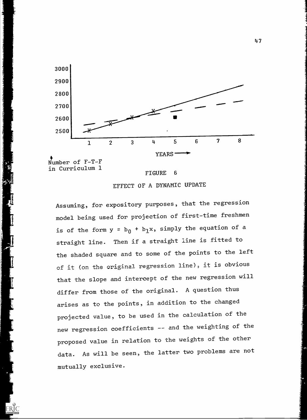
As a very simple example of dynamic updating,

assume that Figure 6 depicts, as in Figure 5, four

years of hard data and four years of projections of

numbers of first-time freshmen in curriculum 1. Again,

the crosses represent hard data, the dots projected

values, and the shaded square the change being instituted.440.

by the model user: the heavy line represents the

original regression line based on the hard data (years 1

through 4).

147

3000

2900

2800

2700

2600

2500

1 2 3 14 5 6 7 8

4Number of F-T-Fin Curriculum 1

YEARS ----4"

FIGURE 6

EFFECT OF A DYNAMIC UPDATE

Assuming, for expository purposes, that the regression

model being used for projection of first-time freshmen

is of the form y = b0 + b1x, simply the equation of a

straight line. Then if a straight line is fitted to

the shaded square and to some of the points to the left

of 41- (on the eNrig;r1=1 Yuzalnc3CCinn liTIP) it is obvious

that the slope and intercept of the new regression will

differ from those of the original. A question thus

arises as to the points, in addition to the changed

projected value, to be used in the calculation of the

new regression coefficients and the weighting of the

proposed value in relation to the weights of the other

data. As will be seen, the latter two problems are not

mutually exclusive.

48

Generally speaking, it would be expected that

the analyst has some reason behind his input of the

changed value, implying that this value is somehow

"important" to the planner in its effects on future

enrollments. Thus the new input value may merit greater

weight in the recalculation of the regression coefficients

than is accorded the other data to be used in the cal-

culations. Three possible approaches to the weighting

of the new value might be as follows:

(1) If the subsequent set of projections is

to be made on the basis of all data from

(relative) years 1 through to the changed

value, each observation would be weighted

exactly as every other. However, each

time an additional point is used as data,

the effect of all points is decreased,

the extent of this decrease depending

upon the total number of points taken as

data.

(2) The new value's importance is implicitely

increased by deletion of the first "few"

observations originally used for the

calculation of regression coefficients.

While the new coefficients would still be

based upon (in our example) 4 observations,

the latter would include all values up to

and including the new value. Thus "few"

49

is defined specifically as that number of

observations which, when dropped, will

leave as "hard" data the same number of

points originally used for calculation

of regression coefficients. It may be

well to note two important facts at this

point: first, that henceforth "hard"

data will mean those data upon which the

regressions are based rather than actual

historical, collected data; and second,

that projected points used as hard data

have the same equation associated with

them as with the original fit to the

collected data. Thus, in Figure 6, it

is not necessary that the change being

input by the model user be instituted in

the first projected year subsequent to

the data of years one through four: the

change might have been input in year

seven, using the collected data of year

four, and the projected points at years

five and six in conjunction with the

input value of year seven for regression.

The trend characteristics developed for

the years one through four data were

transmitted to the points projected for

years five and six. As can be seen, the

50

effect of the changed value on the

calculated trend would not be as diluted

as it was in Case 1, and the calculated

regression line would be, in effect,

composed of the trend inherent in three

collected data points and one assumed or

"changed" point.

(3) To include the capability of more complex

weighting, the model might use weighted

regression, where the solved normal

equations are rewritten 0 = (VVX)-1VVY

where V is a square matrix of weights.

With this technique, the changed value

could be made as "important" as desired

in terms of shifts in the regression

line as a result of its inclusion.

The approach outlined in (2) above is presently

being used as the weighting method. The most important

factor in this choice was from the point of view of the

user of the model, rather than from considerations of

mathematical validity. With method 1, the user could,

in fact would be forced to, perform complicated

calculations in order to give the newly entered value

the desired importance. It seemed thatthe weighting

implicit in the deletion of the most remote observation(s)

was, for small numbers of observations, large enough to

satisfy the user, and obviate the need for him to enter

51

into complicated calculation of the new value required to,

in essence, weight itself. Method (3) was chosen

originally, but the adaptation from batch-processing to

time-sharing use of the model dictated that the computer

memory requirements of the latter be kept relatively

small. Since Method (3) does offer the greatest

flexibility, however, it is recommended that it eventually

be incorporated into the model.

Assume that projections are tn be made on the

basis of the observations on two independent variables:

a "dummy" variable related to the intercept of the

regression line, and "time." The model assumed for the

observations cf Figure 6 is of this form, and thus the

regression lines of that figure have slope and inter-

cept, but no curvature. The original matrix of

observations on the independent variables (the X matrix)

is then of the form

X

where, again,

our example.

1 11 2

1 3

1

u is the number of observations 4 in

Following the procedure outlined in Method

u

(32)

(2), the changed value for some year "p" now becomes

the uth "observation" on the dependent variable, and the

previous u-1 (=3) points are used as the other dependent

variable observations. The X matrix must be changed to

52

1 p-1+11 p-u+21 p-u+3

X (33)

1 p

or, for P=5 and u=4 as in Figure 6;

X = 1 3 (34)

[1

1 41 5

The coupling of the X matrix of (34) with the "observations"

on the dependent variable for years 2 through 5 results

in the dashed regression line of Figure 6. The points

on this line subsequent to the changed year represent the

new set of projections, and have a different trend than

that inherent in the points of the original regression

line. The changed value has been taken to be indicative

of a continuing trend, and the new regression line, in

effect, answers the question "if the changed value had

simply been an actually collected datum, what would have

been the calculated regression line for this dependent

variable, and what effect on the enrollment projections

would this line have had?"

Each time this process is repeated, we say that

an "iteration" of the model has been performed. Changes

may be made in successive or non-successive years, as

long as the latter are in simulated chronological order.

Thus changes might be made in (relative) years 5,7,7,8,

and 10.

53

The dropping of the "oldest" data points brings

up a problem in all cases for which the regression line

does not fit the dependent variable observations

exactly. Previous examples have shown the observations

of the dependent variable to be a segment of a low

order plAynomial expression -- that is, a straight line

fits the data exactly. It is not expected that such

will be the case, and we may assume that the dependent

variable observations might be as shown below, with the

solid line representing the regression based on u=4

observations, the crosses being the actual observations,

and the dots representing projected points on the latter

regression line.

The variable under consideration might be

"numbers of first-time freshmen in curriculum 2" -- and

none of its projected values are being changed by the

model user for this particular iteration. If, however,

changes are being made in "numbers of first-time

freshmen in curriculum 1", the structure of the model

is such that a new regression line will be calculated

for the curriculum 2 freshmen. With no changes being

instituted in the latter, it should be expected that

none of its projected points change. The new

regression line will be calculated on the basis of the

same years' data as the variable actually being changed;

using the example of Figure 7, these years would be

21314, and 5. Using the crosses (in Figure 7) at years

54

2,3, and 4 as the first three "observed" points, and the

dot at year 5, originally a projected point, as the

fourth, it is apparent that the best fit to the latter

four points is the dashed regression line -- resulting

in a new set of projections for years 6,7, and 8 which

differs from the original -- an undesirable situation.

2500

2400

2300

2200

2100

2000

X

X X

I- 1 2 3 4 5 6 7 8

#F-T-F in YEARSCurriculum 1

FIGURE 7

DYNAMIC UPDATE WITHOUT SMOOTHING

The programmed procedure for alleviation of

the situation above is as follows. Prior to projection

for each iteration, the "observations" upon which the

regression coefficients are to be based are "smoothed":

they are placed directly upon the previous regression

line. If, in the next iteration, no "changes" are

desired for a given variable, the "smoothed" data are

taken as observations -- and dropping the "oldest" points

55

doeE; not change the properties of the new line from that

calculated previously. Thus the newly projected values

will equal the old, as they should. Thus in Figure 7,

the heavily shaded circles represent the original data

smoothed -- that is fitted -- to the calculated regression

line: and since these points now have exactly the same

characteristics as the projected points on that line,

the use of a combination of the former and the latter

in the calculation of a new regression line will yield the

old line. In the case of dynamic updating of an element

for which a change has been made, the same reasoning

holds: the data upon which the regression is to be

based must be smoothed to assure a lack of confounding

of the projections based on the change, by the changes

in the regression line due to the use of unsmoothed data.

It may be noted, too, that it is not only in the case

of straight-line projections that the smoothing

procedure must be followed.

C. Data Re uirements of the Model

The previous section has presented a

sophisticated mathematical model; however, the validity

and informational content of its output are a function

of the validity and informational content of the inputs

to it. Thus, while the model may rearrange the input

data in a manner more amenable to analysis, output

validity would require that the output be no more

56

disaggregate than the input data. Therefore, this (or

any) computer model does not produce new information:

it can only rearrange old information; and present it

in a more useful format. However, this procedure must

be prespecified before the computer can begin

processing the data.

The model under consideration produces

enrollment projections. A large part of the projection

process is, in essence, that of fitting curves to a

variety of different sets of data observed over time

and extending these curves into the future. New

information is not produced, but estimates of future

enrollments are made on the basis of that which has

been observed in the past. Therefore, information on

disaggregated projection of enrollments must have its

counterpart in past data. The need of educational

planners for enrollment projections must be balanced

between the desire for a meaningful and comprehensive

format, and the need for enrollment projections in

highly disaggregate form so that planning based on

these projections can be made operational. The person

(or persons) interested in the educational system's

future faculty, facility, and budgetary needs is not

aided by a single "lump" projection of total number of

students in the educational system for some future date.

His immediate questions are "will more students be

attending two-year colleges? Will the proportions of

0 0

0

57

students allocated to each currirmlum be the same? Will

my sector (public or private) gain in enrollment

proportionately with present enrollments, or will

another sector be flooded with students who might

have entered the one with which I am concerned? Will

the programs presently being instated for aid to the

educationally and economically disadvantaged show

significant effect?" The prerequisite to use of a

model which will aid in answering these questions is the

input of data whose disaggregation and information

content corresponds to those outputs which will, in

fact, be such an aid.

Inputs to the model constructed, since the

latter is a prototype, are indicative of the data

requirements of the model which might ultimately be

used as part of the planning function. Since it

was deemed desirable by the educational planners

consulted that projections of future numbers of students

be both classified and categorized (although the terms

used may not have been exactly the same), input data

require both a major classification scheme and a set

of categories of characteristics of students. In

addition, since the worth of the concepts surrounding

transition matrices and the information contained in

the latter were recognized, it was required that

historical transition matrices be obtained.

58

While the form of the input data is somewhat

flexible, there are certain minimum data required for

the running of the model, whose information content

is rigid. From the mathematical structure of the

model, and specifically the recursive relationship

which describes the cycling or aging process, we know

that the total population of the educational system,

grouped both by the major classification scheme and

the categories of characteristics, is cycled through

a transition matrix to yield a similarly classified

and categorized matrix of groups of students who remain

in the educational system for the immediately subsequent

period, To the latter matrix are added two similarly

classified and categorized matrices: one of first-time

freshmen and one of upper-level entrants. The

resulting sum is the total population of the educational

system for that subsequent year, by classification and

category of characteristic. In order for this process

to be carried out by the model for projected years,

the historical data must give information which allows

the components being acted upon by the process to be

developed. Since this development involves the

projection of historical data, the matrices referred

to above must be input for the years in which the

historical data were gathered. Specifically, for each

year for which historical data is to be collected, the

analyst must obtain:

59

(1) a matrix of first-time freshmen, classified

and categorized by the major classification

scheme and categories of characteristics,

respectively, desired by the analyst as

output groupings;

(2) a matrix of upper-level entrants, also

classified and categorized as were the

matrices of first-time freshmen;

(3) a matrix of the transition proportions

between each pair of components of the

major classification scheme and between

these components and the "outside world",

i.e., a transition matrix.

It might be noted parenthetically that if the model is to

be used on a semesterly or quarterly rather than a

yearly basis, the above matrices would have to be

collected for as many periods as were being used for

observation of historical data. Thus for five years of

data on a semesterly basis, ten sets of the above

matrices would be required.

One additional segment of student data is

required for completeness. As is stated in the

description of the recursive relationship, the processing

must start at some point. Because the process is

recursive, a logical starting point is one at which a

matrix of total students, classified and categorized

according to the major classification scheme and

4.

a

Mt

60

categories of characteristics desired for analysis, is

available. Thus it is imperative that such a matrix

is collected for a single year of the historical data;

and it is worthwhile that this year be the first year

for which complete historical data are available. If

this matrix is developed for the first year, one of

the validity checks on the model, designated "concurrent

validity," can be made. In testing concurrent validity,

we are asking the question "does the model (in terms of

the output it produces) represent the present and on-

going function of the system being modeled?" If some

of the historical data are estimates, there may exist

inconsistencies in them. The extent to which these

inconsistencies exist would be determined by comparison

of the simulated results for the historical years with

that which is known to actually have happened. To

reiterate then, the next data requirement would be

(4) for the first period for which complete

historical data are available, a matrix

of total students classified and

categorized as were the matrices of

first-time freshmen and upper-level

entrants.

Also required as input are data concerning

the independent variables upon which the regression

coefficients and ultimately the projected matrices are

to be based. At the very least, the values of all

61

independent variables through time must be input for

both the years to be projected and the historical data

years. For the models run in the time-sharing mode,

as has been stated, core size limitations were such that

the simple reading of the independent variable values

over time would have required too many subsequent

calculations to make the program of feasible length.

Thus the required calculations on the observations

on the independent variables are performed separately

from the computer program itself, and read into the

computer in processed form (where a set of calculations

must be performed for each set of independent variables

which might, during a given iteration of the model, be

used as "observations."). At the same time must be input

each year's values of the independent variables so that

having calculated the regression coefficients, the

projected values of the elements within the necessary

matrices can be calculated. It is in the models run

on the larger core computers that only the sets of

values of the independent variables need be input since

the calculations required for them will be performed

by the computer program itself.

As was indicated at the start of this section,

the form of the input data is somewhat at the direction

of the analyst. Study of the actual program listing by

those knowledgeable in the FORTRAN language will show

the exact input format presently required: this

62

formating is easily changed by the programmer. Thus, for

example, although transition matrix elements are presently

read in percentage terms, the elements might be read in

numerical flow terms and converted by a short subroutine

into the required percentages. In another instance,

the "starter matrix" (classified and categorized matrix

of total students for the first year for which complete

historical data are available) might be read as a vector

of numbers of students by classification, and

associated with each element in this vector a vector of

percentages would be read to convert this (in essence)

starter vector into a starter matrix. Because of the

great number of possible forms in which the data might

be collected, all forms could not be allowed for -- and

thus a single one was chosen which best fit the needs

of the researchers and the data available. Certainly

if the characteristics describing students are not all

of the same variety -- that is, if some are constant

and smite are variable (as discussed in this section

conce-ming evolution of the prototype) some data might

be read as numbers 0± students and others might be

read as percentages of students. The important point

to keep in mind is that regardless of the input form

of the data, they must ultimately be of the form

stated above.

N ti

63

D. Evolution of the Model

As was stated in the general introduction,

the development of the model under consideration

involved a continuous learning process on the part of

all involved. Many of the more tangible results of this

learning are embodied in the computer programs of the

model.

1. Concept Reformulation

As originally conceived, the pilot model would

be small in terms of the number of components in the

major classification scheme and the number of categories

of characteristics describing the student population

of the educational system. It was expected that many

of the operating characteristics of the pilot model

would be incorporated in a more encompassing full-scale

implementation, but that the number of components in the

major classification scheme of the latter would be much

greater than the number in the pilot model. Thus, it

was indicated that a major classification scheme of

two-hundred components was within the realm of

practicality in view of the capabilities of present-day

computing facilities, with perhaps one-hundred categories

of characteristics for description of student populations.

In view of the tremendous data needs of such a large

model, the four pilot applications of the model attempted

611

(Statewide, CUNY, HVCC, RPI) had eight, six, twelve,

and thirty components in their respective major

classification schemes, and nine, twenty-four, two, and

eighteen categories in their respective categorization

schemes. Since one of the facets of the analysis of

the output from these models was that of studying the

trends in transition matri elements over time, it was

found that the output of a given run could reach fairly

large though readily analyzable proportions. Ultimately,

however, it occurred to all concerned that analysis of

a chronologically-ordered array of, say, ten

transition matrices from a model with a major classifica-

tion scheme of two hundred components would involve

some four hundred thousand values: certainly not an

amount amenable to rapid analysis by a single person

or small planning group. Moreover, with the addition

of a one-hundred by two-hundred element array (for each

year) to describe the characteristics of the student

population, 200,000 more numbers await analysis,

bringing the total to more than 600,000 or six-hundred

large pages of computer printout, assuming twenty

columns of fifty numbers each per page. Of course,

all this would be for one iteration of the model, and

even selective printing would yield a prodigious amount

of output at large overall cost. To keep the results

useful, the course taken vas that of considering a

series of less-encompassing models, each permitting

65

analysis of different combinations of components of

that which might be termed the "overall" classification

scheme of the educational system -- a scheme whose

components would include the most disaggregative

delimitations of the system. A series of smaller

models would not only be more amenable to analysis, but

would give more accurate results due to their aggregative

nature. In these studies the structure of the model

would be identical -- only the "labels" associated with

the classifications and categorizations would change.

While this actual use of this new concept some

information would be lost it would not now be possible

to model all the interrelationships among the components

of the overall classification scheme at once -- the

gains in analytic efficacy would appear to far offset

the losses, particularly in light of the fact that

some of these interrelationships might not be of

prime importance to the educational planner. In sum

then, it is expected that the size-range exhibited by

the pilot models developed will more nearly approximate

the size-range of any model actually used as a full-

scale planning aid, as opposed to the rather large

models previously envisioned as full-scale. "Full-

scale" has taken on a new connotation of "flexibility,

capability, and utility," as opposed to that of mere

size.

2. Changes in Inner Structure

A second change in the concept of the model

has direct bearing on the evolution of its inner

structure. As originally conceived, the model would

have associated with each element in a vector of students

by classification a second vector of percentages

representing the proportions of that classification's

students falling into one or more sets of mutually

exclusive and collectively exhaustive categories. These

66

Mai

vectors of percentages were projected as entities

separate from the vectors of first-time freshmen and

the matrices of transition proportions. Determination

of the number of students in each category for a given

projected year and component of the major classification

scheme was then made by multiplying the total number of

students in the component by the projected vector of

percentages associated with the component.

Since at the beginning stages of the research

less consideration was given to the simulative

potentialities of the model, all vectors of percentages could

be considered as a separate projection problem since only

one iteration of the program needed to be made for the

entire set of desired enrollment projections. The researchers

became aware however, that the needs of the educational

planners were such that the simulative capability would

67

be highly important. Therefore much effort was devoted

to the introduction and explanation of the model as a

simulative device with the capacity to aid in evaluation

of policy decisions and exogenous variable changes as

they related to projected college and university

enrollments.

2.1 Introduction of the "Episodic Event"

One of the main operating characteristics of

the simulation model which aids the evaluation of

proposed alternatives and the analysis of the impact of

chance happenings is that of the pvocess of recalculating

the regression curves for projection on the basis of

projections input by the planner. The assumption

implicit in this procedure is that the projection

being input by the planner is to be representative of

some continuing trend. However, as familiarity with

the model on the parts of the planners grew, a question

arose as to the desirability of guaranteeing that input

changes would imply changing trends.

During one demonstration of the model, the

researchers asked for the input of "what-if?" type

questions from the floor: the event decided upon was

that of a one-time influx of black students. In

order to effect this changed projection, the components

of the major classification scheme in which the influx

would be distributed were first determined (by querying

68

the planner responsible for the original question) and

the numerical value of this influx was spread in correct

proportion over the vector of first-time freshmen. A

calculation then had to be performed to determine the

change in the distribution of Negroes. At this point,

the obvious fact was brought out that since the

percentage of Negroes had changed for the freshmen of

a particular year, modeling validity would require

that some change occur in the percentage distribution

of Negroes for the sophomores of the subsequent year --

and that this change would, of course, be a function

of the original change in the percentage distribution.

The model at that time could not handle adequately

this type of a change.

2.2 Matrices of Students

In expanding the capability of the model to

assimilate a "what-if" question of the episodic variety,

a major change was made in the structure of the model:

instead of a vector of classified students whose

elements were each associated with a vector of

categorizing percentages (again, as these terms have

been defined for specific usage in ,this report), the

vector of classified students was expanded into a

matrix of students grouped both by classification and

category of characteristic (See IIA.1., General

Overview, p. 14). Thus in the case of first-time

69

freshmen, a niatrix exists where had previously existed

a vector -- and this matrix was then projected to give

not only the numbers of expected first-time freshmen by

classification, but also by category of characteristic.

This change in the structure of the model set the

stage for the ability of the model to simulate the

episodic event. When the additional influx of students

is input, it is input in raw numerical terms -- and

there are no percentages upon which calculations must

be performed. However, if the simulated students are

described by more than one characteristic, this same

influx must be input into each. Thus, for example, if

one-hundred males are added to the "gender"

characteristic of classification 1; and "age" is a

second descriptor of the simulated students, then

the hundred males added to classification 1 must be

distributed among the categories of age under

classification 1. The aging process then becomes the

cycling of a matrix of students through a transition

matrix, rather than the cycling of a vector through

the transition matrix. As seen in the section concerning

the mathematical derivation of the model, the assumption

of independence between student characteristics and

transition probabilities is highly visible in this newer

though not yet most finalized structure, since a vector

associated with each (fixed) category of characteristic

is cycled through the same transition matrix.

A

70

2.3. Constant, Replarly Variable, and IrregularlyVariable Characteristics

The most recent advance with respect to

categorization of students come with the realization that

while categories such as male, female, and/or "New York

City resident" lend themselves quite readily to the

cycling process described in the mathematical derivation,

categories within such characteristics as "status" or

"age" do not. The fact that a student attends college

on a part-time basis during one time-period does not

necessarily mean that he will do so in the next. The

latter type of characteristic is more correctly included

in the section of the model devoted to student flows

e.g., it should be included in the major classification

scheme rather than as a characteristic. If, however,

flow data on the descriptor in question are not

available or, if available, make the major classification

scheme too large for convenient analysis, certainly some

course of action must be taken. The course chosen was

that of reinstating the separate projection of vectors

of percentages for each component of the major

classification scheme as had been done originally. To

sum up, those characteristics of students which are

relatively constant are cycled through the transition

matrix, while those which can vary in an irregular

manner are projected separately in percentage form, and

later converted to numbers of students by multiplying

71

the number of students in a classification by the vector

of percentages associated with that classification. A

third type of characteristic, one which varies in a

regular manner through time, must be processed as a

function of the manner in which it varies. Thus, for

example, in a model based on one-year time periods age

categories may be spaced in one-year intervals for

simplicity, and these categories cycled through the

transition matrices as in the case of the gender or

geographic origin categories. However, after this aging

process, the number of students in each age category

would have to be shifted to the subsequent age category

so that cycling through the transition matrix would also

have as a result all students being one year older. As

can be seen, the processing of the characteristics of

students would depend on the characteristics themselves,

and a methodology has been developed for each type of

characteristic.

3. Independence of Design from Mode of Operation

A final consideration to be made explicit is

that of the. independence from mode of operation for the

prototype model developed. Originally, only the batch-

processing mode was considered. In an effort to speed

programming and debugging, use was made of a time-

sharing computer service. It should be stressed that

this'han-machine interaction" is a highly desirable

72

feature in the use of a simulation model since

alternatives may be proposed and evaluated almost

instantaneously. Perhaps the greatest usage of the

model would be found in a "real-time environment -- that

is, during actual meetings. Since it was realized that

the interaction between man and computer that had been

by far the most important contribution of the time-

sharing system was an important capability for a

simulation model, the model developed for the analysis

of a particular institution in a "batch" mode was given

an input-output structure adaptable to a time-sharing

mode; an identical structure is maintained in either

mode; the model merely contains the necessary input/

output modifications necessary for communication in

each mode. The same questions are asked, and

similar responses required of the model, in either

of the above two modes. While in the time-sharing

mode the commands and responses of the planner would

be typed directly into the computer via the

teletypewriter, the batch mode requires a deck of

"control cards" which for general usage might be pre-

printed with the queries of the program and punched

just prior to running of the latter. Certainly

several differing versions of the simulation operating

in both a batch and time-sharing mode could be utilized

concurrently. The particular mode of operation utilized

is solely dependent upon the requirements of the user

rather than any exigencies of the simulation.

73

E. An Explanatory Run of the Prototype Model

1. Introduction and Overview

The explanation on the following pages is con-

cerned with the output of the model representing the

New York State educational syst-Im as a whole;* and for

facility of discussion, specific 'referral will be made

to the major classification scheme and categorizations

used. A listing of the results of the run under

consideration is given at the end of this section, and

will be used as the vehicle of the discussion. The

commands and responses of the model user are darkly

underlined to distinguish them from the questions and

responses of the model itself: it will be noted that

the man and the computer are instructed to communicate

in English wherever possible and efficacious,

although the mode of communication is extremely flexible

in computer models in general.

The data for implementation of the statewide

pilot rodel were gathered from a great many sources,

most of which were compiled over the past six years by

the State Education Department, and particularly the

Office of Planning in Higher Education. While a portion

of the data required were available in precisely the

correct form, much did not exist -- particularly those

`Strictly speaking, only the data are thedetermining agents in "as a whole".

74

data concerned with transition proportions. As a result,

many subjective estimates and assumptions were made,

just so that a viable data set could be developed: the

reader is thus cautioned that the results shown in the

output listing are not meant to represent expected New

York State higher educational enrollments for the

coming years, but are meant to represent the form,

content, and usability of the results and model,

respectively.

The subsequent discussion describes in detail

the requests for information, responses of the user,

and type of output involved in a "typical" run of the

prototype model. Generally speaking, the first

iteration performs all projections automatically for a

number of years specified by the first user input.

The first few requests by the computer for information

thus involve giving the user the option of printing or

not printing portions of the projected result. The

"change procedure" of the model is the.1 encountered:

here are chosen the parameters to be changed and the

new assumed future values. Subsequently, the user

chooses the mode of updating the projections (dynamic

or episodic) and is returned to the section of the

model which requests information on those parameters and

variables to be printed.

75

The actual printout begins on page 97. The

discussion follows exactly the order in which the

communications noted above are arranged. Before reading

the text, it may be advisable to skim the printout to

gain at least a sketchy idea of the man-machine

dialogue therein.

2. Discussion

The first question asked of the user is the

number of years he desires to have projected in the

first iteration of the program. Input of the number 8

not only answers the question but determines the

"futuremost" year to be projected: with historical data

for the years 1965, 1966, and 1967 being the foundation

of the projections, the "futuremost" or "max" year as

it will be called, is 1975. For the program under

discussion, up to twelve years might be projected --

a max year of 1979. It might be noted that the three

years' historical data is not a fixed requirement that,

in fact the more years' data used as the basis of the

projections, the more statistical confidence can be

put in the projections.

The user next must choose whether or not to

print the data --Joncerning first-time freshmen. Since he

is viewing the results of the first iteration of the

program, he would, in general, desire to see the

enrollments projected solely on the basis of the

1

76

historical data before they are altered by alternative

assumptions which might be made for the future. In

addition, the first iteration is the only one in which

the opportunity is presented for printout of the

historical data. Since the latter never change, they

need be shown only once.

Wherever possible, the format of the printout

has been made to correspond closely with that found in

already-existing sources of data. After setting up

column headings corresponding to the major classification

scheme which in this particular case is the combination

of college types, controls, and levels pictured in

Figure 8 on the following page, eleven years of "first-

time freshmen by classification" are 'printed -- the

three years of historical data and the eight years of

projections requested. The second group of numbers

is merely a set of aggregations of the above figures

by year for all eleven years: note for example that

for any year, PUB-2YR (public two-year) is the total

of two-year public career plus two-year public transfer

program students for that year in the first group of

numbers.

The next question asked by the program regards

printout of the total number of students in the

educational system, again grouped according to the major

classification scheme, for the projected years and --

in the case of this, the first iteration -- for the

2 Year. Colleges

4 Year Colleges

1

Public

1.Private

Public

Private

FIGURE 8

77

--Career Program (Terminal)

Transfer Program

1-

Career Program

Transfer Program

II.Undergraduate

Graduate

Y7Undergraduate

Graduate

THE MAJOR CLASSIFICATION SCHEME:STATEWIDE MODEL

alp

78

historical years. The user types YES on the teletypewriter,

and the desired printout follows. Again, the major

classification scheme is printed as a convenient reference,

and again are prespecified aggregations printed for each

year. Although it is not necessary that the aggregate

groupings be the same as those for first-time freshmen,

they are the same for this particular model. Again,

it is desirable that "total students be printed for

purposes of comparison with the results of later

iterations.

The user is now queried as to whether he

desires output concerning upper-level entrants, and Fe

must again answer either YES or NO. (Actually any

answer other than YES is interpreted as a negativi.!

response.) Upper-level entrants are grouped by the

major classification scheme, although no aggrr.gation

of them has been carried out However, aggregation

schemes such as those used in the first-tiiie freshmen

and total students -Drintouts are not difficult to

incorporate, and may be installed if desired.

As yet, no mention has been rade of the

categories of characteristics by which students are

described. Following the optional printout of upper-

level entrants, the user may request Euch a printout

for total students by answering YES tc the question

"PRINT STUDENTS BY CHARACTERISTIC?" Data regarding

79

f4rcir-i-ime freshmen and upper-level entrants by category

of characteristic are available and the program can be

modified to print this information.

If the user desires printout on total students

by category of characteristic (and major classification

scheme components), he will then be asked to input the

number of years of output desired, and the specific

dates corresponding to that number of years. In

addition, the user is reminded of the earliest year

available to him for printing. Thus the question of

"how many and which years" is answered by typing 3 (for

three years of output) and the specific years chosen

for viewing, 1967, 1970, and 1975. Two facts must be

noted at this point: first, that the user is reminded

of the earliest year avaiable to him for viewing -- in

the first iteration it is the first year from which

historical data have been utilized, while in subsequent

iterations, it is the changed year, since output from

before the changed year would exactly equal that from

the previous iteration. Secondly, that in comparison

to batch-processing systems in general, on-line

printing is quite slow. The six-line per minute typing

speed of the teletypewriter makes it imperative that

the user have the option of specifying some portion'of

the output which is most critical to his needs, and not

printing all those results which he might. For some

segements of the potential output, a considerable time-

80

savings can result from this option: the three years'

results shown took approximately six minutes to print; a

total printout at this point would have taken about 16

minutes.

The printout of total students by classification

and category of characteristic is preceded by the

printing of a key so that each years' set of numbers can

be understood. Thus the nine categories of characteris-

tics are read from the key: the categories are male,

female, full-time, part-time, U.S., foreign, residence

in same county as school attended, residence in same

economic area (excluding county) as school attended,

and finally, residence in New York State other than

economic area of school attended. The characteristics

are sex, status, and geographic origin; since the key

states that these categories are found "reading down," the

first row of the printout represents "male," the second

row, "female," and so on. Thus, for example, the

upper-left-hand corner element of the first (1967)

matrix of values indicates that in 1967 there were 34,478

males in career (terminal) programs in the State's

two-year public schools. Furthermore, it is seen by

the third (1975) matrix printed that there will be

63,606 such students by 1975.

Having printed the total students by category

of characteristic for- the desired years, the user must

answer YES or NO to the question of whether or not to

81

print any transition matrices. For the reasons iterated

in the case of categories of characteristics, the user

can choose the specific years he is most highly interested

in, and have those years only printed out.

Accordingly, he answered YES to the question of

whether or not to PRINT TRANSITION MATRICES, and three

years were indicated: 1968, 1970, and 1975. Again,

as with all printout on the first iteration, the

earliest year available is the first year of historical

data.

In viewing the printout of the transition

matrices, the user must recall that the quantities

within them represent flows or movements of students

between all the components of the major classification

scheme delineating the possible student locations within

the educational system. Thus before actual printout of

the matrices themselves, the user is reminded that the

row headings are those of the first eight columns,

ordered in the same manner as the order of the column

headings. It may be well to note that this ordering

is exactly the same as that inherent in the printout of

first-time freshmen, total students, and upper- level

entrants. The headings (understood) for the rows, and

the abbreviated headings for the columns then represent,

in order, two-year public career (2PC) two-year public

transfer (2PT), two-year private career (2PRC), and so

forth. The last two columns of the matrix of transitions

82

should be interpreted as "those who leave the educational

system without a degree," and "those who leave the

educational system with a degree," respectively.

While for computational purposes the elements

within the transition matrices must be in percentage

form, it was felt that for purposes of analysis, more

meaning could be gained if printout were in terms of

"numbers of students" making the component-to-component

transitions, and this conversion is made prior to output.

Associated with each year is a transition

matrix. The convention adopted was that the associated

year would be the "first term" in the actual academic

year. Thus the first matrix printed, that for 1968,

represents transitions over the academic year 1968-1969.

In this "1968 transition matrix," the numbers represent

projected inter-component flows of students. Reading

across the first row of the matrix, of the total number

of students in two-year public schools, in career

programs in 1968, 22,597 remained in that classification

for the start of 1969; 3,507 switched to transfer pro-

grams within the two-year public schools; 133 remained

in the career program but switched to private schools;

133 switched to the transfer program at private two-

year schools; 999 became undergraduates at public 4-year

colleges; none became graduate students, 564 became

undergraduates at private four-year colleges, 32,651

left the system with a degree. If all the latter numbers

83

are summed, it will be found that the result is 66,593

the number of two-year public career students in the

educational system in 1968 as previously printed.

Analysis of each of the rows in turn, (two-year public

career, two-year private transfer, and so forth) would

be performed in the same manner, for each transition

matrix.

Transition matrices are the last projected data

Printed by the prototype at present. At this point we

may say that the first iteration of the program has

ended: a complete set of projections has been made,

although to save printing time, only the "important"

ones have been viewed. The word "important" has been

put in quotes since the printout being shown was the

result of a run made purely for explanatory purposes.

In an actual planning situation, however, it is assumed

that the user of the model will be concerning himself

with specific portions of the total potential output,

and thus there will be different measures of

"importance" associated with different portions of

printout in different runs, and, for that matter,

iterations of the same run.

The user is now queried as to whether he

desires to make another set of projections, implying

the question "are changes to be made in projected

values for analysis of their impact on system variables?"

Put another way, "does the user wish to evaluate the

84

effect on projected enrollments of some policy change(s),

change(s) in the environment exogenous to the

educational system, student behavior change(s) or

resource allocation change(s)?" In the present form of

the model, these changes would be input in terms of

changes in the quantities of first-time freshmen, or

upper-level entrants for a given year or years; or in

terms of changes in the transition proportions for a

given year or years. This change procedure is such

that only the values of a single year's projections can

be changed in a given iteration -- although the use of

the dynamic updating procedure allows for changing

overall trends by insertion of only one years' changed

values.

In view of the above, the user having answered

YES to the question of whether another set of

projections was desired, the program then asks for that

year in the future for which a set of changes is to be

made. Before explaining the output listing any

further, however, it will be quite helpful if the

question being asked is described in-detail. In

relation to the type of questions that might be

asked by educational planners, the following will

appear highly simplified, and rightly so: the problem

was conceived solely for the purposes of this

explanation.

84

effect on projected enrollments of some policy change(s),

change(s) in the environment ekegehOUS to the

educational system, student behavior change(s) or

resource allocation change(s)?" In the present form of

the model, these changes would be input in terms of

changes in the quantities of first-time freshmen, or

upper-level entrants for a given year or years; or in

terms of changes in the transition proportions for a

given year or years. This change procedure is such

that only the values of a single year's projections can

be changed in a given iteration although the use of

the dynamic updating procedure allows for changing

overall trends by insertion of only one years' changed

values.

In view of the above, the user having answered

YES to the question of whether another set of

projections was desired, the program then asks for that

year in the future for which a set of changes is to be

made. Before explaining the output listing any

further, however, it will be quite helpful if the

question being asked is described in-detail. In

relation to the type of questions that might be

asked by educational planners, the following will

appear highly simplified, and rightly so: the problem

was conceived solely for the purposes of this

explanation.

85

One of the great concerns of our hypothetical

planner (the "user" heretofore referred to) may be the

interface between the public and private sectors of

the educational system. He has heard rumored that

another year or two will see a very significant tuition

increase for undergraduate students at private four-

year colleges in the state, and it is his feeling that

many of the students who enter the state higher

educational system at other than the freshman level who

would ordinarily have come into the private sector will

enter the public sector instead. Generally speaking,

he wishes to see the impact on higher educational

enrollments in both sectors subsequent to this tuition

increase. It might be noted that although this is a

hypothetical problem, real problems of this nature have

been forecasted.

It is the analyst's option that only full-

time rather than part-time students will be affected

by the increased tuition; in addition, that male

students rather than females will be affected by it; and,

finally, that the effects will be such that in the

year following the tuition increase, the tuition will

be brought back to its former level, i.e,, that the

increase in tuition will be an "episodic event," as

will be the influx of students from the private to the

public sector. Given the size of the rumored increase,

the planner expects that in the year of the tuition

86

change (most probably 1970), upper-level entrants into

the private colleges' four-year undergraduate programs

will be fewer by ten percent than the number projected

for that :;ear.

The planner has now defined his question in

operational terms with regard to the inputs required to

ask it of the computer model. Returning to the

original projection of uppeP-level entrants into the

four-year private schools (undergraduate level) he

finds that the former was 29,996, ten percent of which

is approximately 3,000.

In answer to the question regarding "year of

the change," the planner responds 1970 -- the year in

which he expects the tuition increase. After the model

reminds the user of the codes (and identifying

characteristics) of the variables available for change,

of which there are three, he is asked to punch the code

number of that variable in which changes will be made --

in this case upper-level entrants, code 3. Referring

back to the major classification scheme (always present

for any block of output) he determines that four-year

public school students at the undergraduate level

always appear in the fifth column of printout -- thus

making the coded classification of the latter students

"5". The categories of characteristics with which the

planner is most concerned are "male," "full-time," and

"resides in U.S. other than New York State." The coding

87

scheme for categories of characteristics has a one-to-

one correspondence with the order in which they are

printed: since the order is male, female, full-time,

part-time, resides in U.S. other than N.Y., and so

forth, changes must be made in 3 categories 1, 3, and

5. (It must be noted that for simplicity, it has been

assumed in this example that an entrant into the

educational system at some level above freshman must

reside outside New York State. Obviously, such is not

necessarily the case -- a New York resident may start

college in another state and during some later year

transfer back into his home-state's educational system.)

Of course, changes might have been made in all nine

categories if both males and females, both full and

part-time students, and students from all geographic

origins were felt to be affected by the postulated

tuition change. In this case, the input would have

been 5,9,1,2,3,4,5,6,7,8,9.

The planner is then instructed to input the

increases or decreases corresponding to the categories

he has specified. For the case in point, the planner

is adding three-thousand male, full-time, non-New York

residents, i.e., 3,000 male, 3,000 full-time, and 3,000

non-New York, in terms of the structure of the model.

(The word DELETED is printed by the time-sharing

system if the user indicates that he has made a mistake

88

by punching a certain combination of keys. Since it

was not desired that 30,003 full-time students be added,

the entire line of input was erased by punching that

combination.)

The next question asked by the computer is

whether other changes are going to be made on the same

variable, the latter currently being upper-level entrants.

The planner has yet to decrease the four-year private

college (undergraduate) upper-level entrants by 3,000,

so he still desires to make changes in variable 3. He

thus types YES to the question SAME VARIABLE? Again

referring to the major classification scheme, the code

of the four-year private undergraduates is 7. The

number of changes to be made is 3, and the codes of the

categories (element codes) are the same since the

simulated students will not change their sex or

geographic origin is going to public rather than to

private schools. Another assumption being made is that

the private sector is being depleted only in terms

of full-time students. The input is thus of the form

7,3,1,3,5, and, again, the changes (now decreases) are

-3,000, -3,000, -3,000. No more changes are to be

made in upper-level entrants, and, in fact, no other

variables are to be changed. As can be seen in the

sample output, a "4" is punched by the user in answer

to the question concerning the code number of the next

variable to be changed. Finally, since the event whose

89

effects are to be analyzed is assumed episodic, the user

commands that the episodic updating procedure be utilized

for the next set of projections by typing "2" when asked

for orders.

At this point, the entire printout cycle

begins anew. Since it was assumed that the number of

entering first-time freshmen would not be affected by

the tuition change, there is no need to waste time

printing first-time freshmen again; and the response to

the printout query is NO. It is, however, expected

that the total student population will change, if

not in numbers, at least in distribution of numbers:

thus it is printed. Setting aside the printout of

total students for a moment, it will be noted that a

printout of entering students was called for: the

purpose here was to indicate the effect of the episodic

updating procedure. As will be noted, only two

numbers have changed between 1970 and 1975; and no

printout is available for the years prior to the change.

In the case of the latter, since the future does not

affect the past, there will never be any effect in

those years prior to the year in which a change has

been instituted: thus these prior years are not

printed. In the instance of the effects of the

episodic update, by definition, the loss of 3,000

students by the private sector in 1970 (from 29,996 to

26,996) gained by the public sector in that year (from

90

21214 to 24214) is a one-time affair with no after effects

on the future viz., 1971 projections of upper-level

entrants, and thus the latter remain as they were in

their previous printout.

Returning now to the output of total students

(again, printed only for those years for which the

change may have effect), careful comparison must be

made with the original total student printout. It is

the planner himself who can best judge the results, and

detailed analysis of them will nct be attempted here.

It may be well to note, however, some general points of

comparison. First, of course, is the fact that the 1970

projections differ only in that four-year public

undergraduate enrollments have increased by 3,000 (from

171,706 to 174,706) and four-year private undergraduate

enrollments have decreased by a like number (from 248,454

to 245,454). Second, that the aggregates (the second

block of printout) have been updated accordingly. Third,

that in 1971 the distribution of enrollments is quite

different from what it was before, and that the 1971

grand total is lower in the new projections due to

higher attrition and/or higher percentages obtaining

degrees in the public sector. Fourth, that the influx

of students in the public sector, and "outflux" of

students in the private sector add an impulse and cause

a gap, respectively, in the enrollments of the graduate

schools for which the undergraduate schools are a

91

primary source; and finally, that the perturbation dies

out over time as the equilibrium of the system is re-

established.

The next question that arises is that of

change in the student population with regard to

categories of characteristics by which they are described.

After answering in the affirmative the question by the

computer of whether or not to print this breakdown of

the population, the user is instructed that the earliest

year available for printout is 1970 (the year in which

the change was instituted), Briefly, the two years

desired, 1970 and 1975, are printed. As expected the

four-year public undergraduates show an increase in

the number of male students in 1970 (81,176 to 84,176) of

3,000, as do full-time and non-New York residents.

The four-year private undergraduates have 3,000 fewer

males, and so forth. By 1975, the differences between

the original projections and the new ones have become

small, although the differences in the transition

proportions between the public and private four-year

schools and the two-year schools (some flow from four-

year to two-year is indicated by the historical data)

have changed the sex, status, and geographic origin

distributions in the two-year public schools to an

extent.

It is analysis of the transition matrices

which gives exact information as to the changes seen

92

in the projections of total students in the years

subsequent to the year in which the changes in variable

values were made. While the thrust of the possible

analysis will not be discussed, the approach would, again,

be that of comparison of the present results with those

of the prior iteration. Thus, for example, the reason

that the 1971 figure for total two-year public school

(career) students went from 90,918 in the first

iteration to 90,970 in the second is seen in the first

column of the 1970 (representing 1970-1971) transition

matrix: when compared to that obtained for the first

iteration, this change is small, but will be used for

expository purposes. In the latter, the number of

students moving from four-year public undergraduate to

two-year public (career) for the following year was

5,134; from four-year private schools there were

3,123. Since it was assumed that 1970 would see 3,000

fewer four-year private-school undergraduates, it is

to be expected that there would be fewer of the latter

moving to the two-year public (career program) for 1971:

such was the case, and the second iteration result was

that only 3,086 four-year private undergraduates

switched to two-year public schools (career program)

for 1971 -- a decrease of 37 students. On the other

hand, with 3,000 additional undergraduates in the four-

year public schools, it was to be expected that there

would be a greater number of the latter moving to the

frA

93

two-year public schools (career program) for 1971:

such, too, was the case, and the second iteration

resulted in 5,224 studs making this move an increase

over the original 5,134 of 90 students. The net gain

for the two-year public school career program was thus

90-37 or 53 students -- the difference (within the

limits of round-off error) between 90,918 and 90,970.

It might be well to note at this point that

the detailed explanation of an analytic process is

generally longer than the process itself. As stated

previously, the model under consideration is a prototype:

experience with it will indicate methods by which the

analytic procedures required for its use can be simpli-

fied -- perhaps by different formatting of output, or

different arrangement of same.

The program has at this point reached the

end of the second iteration. The number of iterations

is not constrained by the program per se, but rather by

considerations of the planners' time and costs. If the

word NO were answered in response to IS ANOTHER SET OF

PROJECTIONS DESIRED? the progrzi.m would end. The word

YES has been entered, however, and . 'lay be assumed

that another set of assumptions concerning the future

is about to be implemented in the simulated educational

system.

94

F. Concerning Predictive Accuracy

As was stated in the brief introduction to this

explanatory run, the results given are not meant to

represent New York's higher edudational enrollments over

the coming year.

While the process performed by the model to

age student populations appeals to our sensibilities as

truly representative of that which occurs in an

educational system, by no means may we fairly evaluate

its predictive accuracy as yet. In addition to the

aging process, there is a second main component to the

student population projections -- development of the

projected transition matrices and matrices of first-

time freshmen and upper-level entrants. As has been

stated, the latter "development" is accomplished

through the use of multiple regression models which

relate some set of independent variables to the

(dependent) variables under study through an equation

or set of equations. The dependent variables are well

defined in the prototype under consideration; they

are the elements of the three types of matrices just

mentioned. The independent variables are not so well

defined -- in fact they are undefined until research

has been undertaken'to discover those variables which

appear to be related to the dependent variables.

Moreover, the nature of this relationship must be

95

determined so that the resulting regression equation will

mirror the relationship to the real world.

Such research has not been undertaken in the

present work. Had it been, there might have been

reference to such independent variables as Gross

National Product, median yearly income in the State, and

population growth; and allusions to different alterna-

tive functional forms relating these variables to the

dependent variables in question. Thus, for example,

a viable regression model for projection of first-time

freshmen might be a function of time, of the logarithm

of G.N.P., the square-root of the population of New

York, and the reciprocal of military spending.

Obviously, the number of possible regression models is

limitless: the problem is finding one that fits the

historical data to the greatest extent possible without

"overdetermination" -- that is, the use of too many

independent variables, with consequent obviating of

statistical validation. The model thus should not

be evaluated on the basis of the numbers it has produced

to date. As has been stated in a previous section,

the regression model used was that of a straight line

a slope and an intercept -- based entirely on the

passage of time. While time will surely prove to be an

important independent variable, possibly the most

important, it may be found that the introduction of

other independent variables into the regression model

96

will make the regression equations fit more closely the

histoPical data, and possibly improve the projections.*

That the aforemmtioned research was not done

was neither an oversight nor an error. The model under

consideration is only a prototype: it possesses the

basic wherewithal for projection of higher educational

enrollments. Our basic purpose thus becomes one of

evaluating its operating characteristics in an actual

planning environment, and its capabiliT.y of fulfilling

some of the needs of the planners themselves so that they

can be better equipped for the performance of their work.

Once it has been decided that the model can, in fact,

be useful, then it will be more appropriate to conduct

further research into the actual structure of the

projection relationships.

*It was recognized that a large degree of

auto-correlation may, and quite possibly does, existbetween the assumed dependent variates. As stated,however, the emphasis at this stage of development hasbeen directed toward an assessment of the overallviability and "usefulness" of the model in a planningenvironment.

APPENDIX 2.A

97

SAMPLE OUTPUT

NO. OF YRS. TO PROJECT?8

PRINT FIRST TIME FRESHMEN?(YES OR NO)?YES

YEAR

TWO-YEARPUBLIC PRIVATE

CAR TRANS CAR TRANS

FOUR-YEARPUBLIC PRIVATE

UND GRAD UND GRAD

1965 19838. 19838. 1668. 1668. 33052. O. 49827. 0,

1966 22300. 22300. 1715. 1715. 31700. 0. 49500. O.

19 67 25100, 25100. 17.60, 1760. 3A600. O. 51900. 0.

1968 27675. 27675. 1806. 1806. 34665. O. 52482, 0,

1969 30306. 30306. 1852. 1852. 35439. 0, 53518. O.

1970 32937. 32937, 1898, 1898. 36213. 0. 54555. O.

1971 35568.. 35568. 1944. 1944. 36987. O. 55591. 0.

1972 38199. 38199. 1990. 1990. 37761. C. 56628, 0,

'1973 40830. 40830. 2036. 2036, 38535. O. 57664, 0.

1974 43461. 43461, 2082. 2082. 39309. 0. 58701. 0,

1975 46092. 46092. 2128. 2128. 40083. 0. 59737. O.

YEAR PUB-2YR PRI-2YR PUB-4YR PRI-AYR TOT-2YR TOT-AYR GRAND TOT

1965 39676. 3336. 33052. A9R27, 43012. 1'2879. 125891.

1966 44600. 3430. 31700. 49500. 48030. 81200. 129230.

1967 50200. 3520. 34600. 51900. 53720. 86500. 1A0220.

1968 55349. 3613. 34665. 52482. 58962. 87147, 1456109,

1969 60611. 3705. 35439. 5351?. 64316. 88958. 15327A.

1970 65873. 3797. 36213. 54555. 69670. 90768. 160438.

1971 71135, 3889, 36987. 55591. 75024. 92579. 167603.

1972 76397. 3981. 37761. 56628. 80378. 94389. 1745767,

1973 81659. 4073. 38535. 57664. 85732. 96200. 181932.

1974 86921. 4165. 39309. 58701. 91086. 98010. 189096.

1975 92183. 4257. 40083. 59737. 96440. 99821. 196261.

PRINT TOTAL STUDENTS?YES

98

TWO-YEAR FOUR-YEARPUBLIC PRIVATE PUBLIC PRIVATE

YEAR CAR TRANS CAR TRANS UND GRAD UND GRAD1965 48977. 48978. 3590. 3590. 157944. 23132. 224803. 57899.1966 54269. 54346. 3653. 3623. 150971. 36753. 218322. 75990.1967 58096. 58276. 3701. 3704. 158564. 40703, 224684. 80002.1968 66593. 67616. 3789. 3794. 159557. 45683. 232468. 88567.1969 74192. 74983. 3900. 3892. 165183. 55108. 239382. 95511.1970 82296. 82947. 4012. 3999. 171706. 60987. 248454. 101555.1971 90918. 91332. 4128. 4110. 178752. 66402, 2513991. 107025.1972 100030. 100065. 4247. 4226. 136042. 71416. 270499. 112086.1973 109612. 109095. 4370. 4344. 193375. 76073. 282636. 116813.1974 119647. 118382, 4496. 4463. 200618. 80408. 295169. 121232.1975 130127. 127887, 4624. 4583. 2076E33. 84446. 307946. 125349.

YEAR PUB-2YR PR1-2YR PUB-4YR PRI-4YR TOT-2YR TOT-AYR GPAND TV?1965 97955. 7180. 131076. 282702. 105135. 463778. 558q13.1966 108615. 7276. 187724. 294313. 115891. 482036, 597928.1967 116372. 7405. 199267. 304686. 123777. 503954. 627731.1968 134209. 7583. 208239. 321034. 141792. 529274, 671066.1969 149175. 7792. 220291. 334893. 156967. 555184. 712151.1970 165243. 8010. 232693. 350009. 173254. 582702. 755956.-1971 182250. 8238. 245155. 366016. 190488. 611170. 801658.1972 200095. 8473. 257457. 382586. 208568. 640043. F48611.1973 218707. 8714. 269448. 399449. 227421. 668'897. 896313.1974 238029. 8959, 281025. 416402, 246988. 697427. 944415.1975 258014. 9207, 292129. 433295. 267222. 725424, 992646.'PRINT UPPERCLASS ENTRAPTS?YES

YEAR

TWO-YEARPUBLIC PRIVATE

CAR TRANS CAR TRANS

FOUR-YEARPUBLIC PRIVATE

UND GRAD UND GRAD1965 952. 1020. 214. 220. 6276. 3140. S092. 4263.1966 970. 1105, 234. 190, 7376. 10412. 10945. 13185.1967 1062. 1396. 195. 232. 12521. 5978. 17072. 8215.1968 1105. 1550. 195. 226. 14969. 9348. 2101. 19507.1969 1160. 1738. 186. 232. 18092. 10767. f.5506. 14483.1970 1215. 1926. 176. 238. 21214. 12186. 29996. 16A59.1971 1270. 2114. 167. 244. 24337. 13E05. 34436, 18435.1972 1325. 2302. 157. 250. 27459. 15024. 38976, 20411.1973 1380. 2490. 148. 256. 30582. 16443. 43466. 22387.1(374 1435. 2678. 138. 262. 33704. 17862. 47956. 24363.1975 1490. 2866. 129. 268. 36827. 19281. 524w, 26339.

99

PRINT STUDENTS By CHARACTERISTIC?YES

110W MANY. YEARS OF OUTPUT, AND WHICH YEARS(EARLIEST YEAR CAN BE 1965)?3,1967,1970,1975

READING DOWN THE ORDER IS:MALE,FEMALF,FULL-TIME,PART-TIME,U.S. OTHER THANNEW YORK STATE,FOREIGN,RESIDES IN MINTY OF SCHOOL,RESIDES IN ECO. AREA (EXCL. COUNTY) OF SCPOOL,RESIDES IN NEW YORK BUT NOT ECG. AREA OF SCHOOL.

YEAR 1967

TWO-YEAR FOUR -YEARPUBLIC - PRIVATE PUBLIC PRIVATE

CAR TRANS CAR TRANS UND GRAD UND GRAD52240.2776242527.37475.10512.1607

48290.3726,15863.

34478. 34357. 1887. 1916. 84808. 22364. 141676.23617. 23920. 1814. 1788. 73756. 18339. 83008.31970. 34167. 2969. 2963. 117065. 16872. 181038.26125. 24109. 732. 741. 41499. 23832. 43647.2609. 3556. 1280. 1216. 5030. 1562, 54874.361. 454. 65. 65. 933. 302. 5864.

35971. 36015. 1009. 1120. 11955g. 30216. 114211.7095. 6457. 263. 261 . 10480. 2562. 8814.11116. 10877. 1085. 1042. 22525. 5946. 40971.

CARPUBLIC

TRANS

TWO-YEARPRIVATE

CAR TRANS44360. 45445. 2068. 2082.37936. 37503. 1944. 1917.47212. 51343. 3137. 3131.35086. 31607. 877. 867.4433. 6996. 1340. 1286.439. 728. 66. 68.

49206. 48844. 1146. 1224.9575. 8441. 302. 255.15440. 15335. 1141. 1102.

YEAR 1970

FOUR-YEARPUBLIC PRIVATEUND GRAD UND GRAP

81176. 33314. 154512. 3S7490530. 27673. 93942. 37681128439. 28821. 1992S4. 5881643267. 32166. 49170, 427406470. 3177. 59588. 13984898. 528. 6815. 2038

127790. 43965. 127471, 6116511214. 3761, 9672. h751

25020. 9091. 45363. 19627

100

CARPUBLICTRANS

TWO-YEARPRIVATE

CAR TRANS

YEAR 1975

FOUR-YEARPUBLIC PRIVATE

AND GRAD ID!D GRAD63606. 65495. 2387. 2389. 82213. 44221. 187044. 76Q21.66522, 62392. 2237. 2193. 125470, 40225. 4Fh29,77263. 82127. 3452. 3452. 158035. 40352. 245330. 68523.

52873. 45766. 1178. 1131. 49649. 44093. 62617. 56827.

8379. 12985. 1487. 1449. 8242. 4632. 72400, 16391.

619. 1275. 74, 735. 742. 8957, 2571.

75001. 72502. 1369. 1394. 153722. 60148. 159334, 75833.

14488. 12086. 371. 259, 13271. 5147. 11693, 5731.

24130. 23535. 1271. 1238. 30803. 12676. 56424. 24833.

PRINT TRANSITION MATRICES?YES

HOW MANY YEARS OF OUTPUT; AND WHICF YEARS(EARLIEST YEAR CAN BE 1965)73 1968,1970,1975

FIRST EIGHT ROW HEADINGS SAME AS FIRST EIGHTCOLUMN HEADINGS. LAST TWO COLUMNS ARE ACADEMICATTRITION AND 'LEFT WITH DEGREE', RESPECTIVELY

2PC 2PT

22597.13304.

15.8.

4436.0.

2367.0.

2PC

28584.17215.

16.8.

5134.O.

3123.O.

YEAR 1968

2PRC 2PRT 4PU 4PG 4PRU 4PRG ow DEG

3507. 133. 133, 999. O. 564. 0. 32651. 6009.

18909. 137. 137. 5322. 0. 747. O. 28226. 834,

95. 955. 409. 25. O. 115. O. 1511. 664.

8. 637. 842, 75. O. 532. n, gs.z,

7840. 0. 106. 99989. 6382. 3670. 6595. 15748. 14791.

0. 0. 0. O. 33467. O. 227. 5846. .1 .agA9..

12502. O. 180. 5243. 2996.154729. 12956. 19727. 21689.

0. 0. 0. O. 1496. O. 61249. 9156. 16666.

YEAR 1970

2PT 2PRC 2PRT 4PU 4PG 4PRU 4PRG OW DEG

4005. 165. 165. 1234. O. 1092. O. 39609. 7449.

23047. 169. 169. 6446. 0. 1296. O. 33557. 10AR.

100. 1011. 433, 31. O. 122. O. 1595. 703.

8. 672. 88S. 33. O. 561. O. 1707, 72,

8454. O. 80.104168. 7212. 4293. 5410. 18493. 17462.

O. O. 0. O. 40278. O. 407. 8056. 12246.

18037. O. 187. 5466. 3592.161550. 12571. 21082. 226 47,

O. O. 0. O. 1715. 0, 69202. 1091C. 19726.

2PC 2PT 2PRC

47800. 5032. 260.30087. 34943. 266,

i8, ii6, 1165.9. 9. 770.

2PRT 4PU

260. 1952.266. 9614.49c1, A741017. 106.

YEAR 1975

4PG 4PRU

O. 3288.O. 3503.n. 1110,

0, 643.7300. 10277. O. 0.115606. 9761. 6230.

O. O. O. O. 0, 50067. O.

55634 35427. O. 219. 6383. 5563.189354.Os O. 0, 0. 0, 2117. C.

IS ANOTHER SET OF PROJECTIONS DESIRED?YES

101

4PRG OW DEG

O. 59702, 115333.O. 47492. 1716,0, 1827, 811,O. 1945, 82.

5676, 27039, 25793,986, 13689. 1a703.

11946. 26126. 27366,82239. 14737. 26256.

FOR WHAT YEAR ARE CHANGES IN PROJECTED VALUES TO BE MADE?1970

1. TRANSITION MATRIX(ROW,COLUMN)2, FIRST-TIME-FRESPMEN(SCFOOL/STATM,CPARACTERISTIC)3. UPPERCLASS ENTRANTS(SCHOOL/STATUS,CHARACTERISTIC)

PUNCH CODE NUMBER OF VARIABLE TO,BE CHANGED. PUNCH 4 IF NO MORE CHANGES TO BE MADE.?3

PUNCH CODED CLASSIF., NO. OF CHANdES,ELEMENT CODES?5,3,1,3,5

PUNCH THE 3 INCREASE(S),DECREASE(S)?3000,30003 DELETED

3000,3000,3000

SAME VARIABLE?YES

PUNCH CODED CLASSIF., NO. OF CHANGES,ELEMENT CODES?7,3,1,3,5

PUNCH THE 3 INCREASE(S),DECREASE(S)?-3000,-3000,-3000

SAME VARIABLE?N0

PUNCH CODE NUMBER OF VARIABLE TOBE CHANGED. PUNCH A IF NO MORE CHANGES TO BE MADE.?4

INPUT CODE NO. OF METHOD FOR NEXT PROJECTIONSPUNCH 1 IF DYNAMIC UPDATE, 2 IF EPISODIC UPDATE

PUNCH 3 TO END THE RUN. ORDERS?2

PRINT FIRST TIME FRESHMENUYES OR N0)?N0

PRINT TOTAL STUDENTS?YES

102

YEAR

TWO -YEARPUBLIC PRIVATE

CAR TRANS CAR TRANS

FOUR-YEARPUBLIC PRIVATE

UND GRAD UND GRAD

1970 82296. 82947. 4012. 3999. 174706. 60987. 245454. 101555.

1971 90970. 91262. 4128. 4110. 180507. 664535. 257115. 1069g5.

1972 100062. 99981. 4247. 4225. 187043. 71515. 269339. 112032.

1973 109620. 109018. '4370. 4343. 193931. 76161. 281924. 11675g,

1974 119640. 118318. 4496. 4462. 200918. 80474. 294736. 121183.

1975 130113. 127838. 4624. 4582* 207839. 84492. 3076R3. 125308.

YEAR PUB2YR PRI2YR PUB4YR PRI4YR TOT2YR TOT4YR GRAND TOT

1970 165243. 8011. 235693. 347009. 173254. 582702. 755958.

1971 182232. 8237. 246991. 364100. 190469. 611092. 801561.

1972 2000430 8472. 258558. 381370. 20:1515. 639929. FASAAA,

1973 218638. 8712. 270092* 398682. 227350. 668774. 896125.

1974 237958. 8958. 281392. 415919. 246916. 697311. 944226,

1975 257951. 9206. 292330. 432992. 267157. 725322. 992479.

PRINT UPPERCLASS ENTRANTS?YES

YEAR

TWO-YEARPUBLIC PRIVATE

CAR TRANS CAR TRANS

FOUR -YEARPUBLIC PRIVATE

UNP GRAD UND GRAD

1970 1215. 1926. 176. 238. 24214. 12186. 2699g. 164544.

1971 1270. 2114. 167. 244. 24337. 13605. 344E6. 18435.

1972 1325. 2302. 157. 250. 27459. 15024. 3897g. 20411.

1973 1380. 2490. 148. 256. 30582. 16443. 43466. 22337.

1974 1435. 2678. 138. 262. 3370, 17862, 47956. 24363,

1975 1490. 2866. 129. 26E. 36827. 19281. 52446. 26339.

PRINT STUDENTS BY CPARACTERISTIC?YES

HOW MANY YEARS OF OUTPUT, AND WHICH YEARS(EARLIEST YEAR CAN BE 1970)?2,1970,1975

READING DOWN THE ORDER IStMALE,FEMALE,FULLTIME,PARTTIME,U.S. OTHER THAN

NEW YORK STATE,FOREIGN,RESIDES IN COUNTY OF SCHOOL,RESIDES IN ECO. AREA (EXCL. COUNTY) OF SCHOOL,RESIDES IN NEW YORK BUT NOT ECO. AREA OF SCHOOL.

CARPUBLIC

TRANS

TWO-YEAR

CARPRIVATE

TRANS

103

YEAR 1970

FOUR-YEARPUBLIC PRIVATEUND GRAD IIND GRAD

44360. 45445. 2068. 2082. 84176. 33314. 151512. 63$7h,37936. 37502. 1944. 1917. 90530. 27673. 93942. 37681.47212. 51343. 3137. 3132. 131439. 28821. 196284. 59816.35086. 31607. 877. 867. 43267. 32166. 49170. 42739.4433, 6996. 1340. 1286. 9470. 3177. 56588. 139134,

439. 728. 66. 898. 528. 6815. 2039149206. 48844. 1146. 1225. 127790. 43965. 127471. 61165.9575. 8441. 302. 255. 11214. 3764. 9672. 4751.15440. 15335. 1141. 1103. 25020. 9091, 45363. 19627.

CARPUBLIC

TRANS

YEAR 1975

TWO-YEAR FOUR-YEARPRIVATE PUBLIC PRIVATE

CAR TRANS UND GRAD UND GRAD63591. 65446. 2387. 2389. 82369. 44267. 186782, 76880.66522. 62392. 2237. 2193._ 125470. 40225. 120901. 49429.77248. 82078. 3451. 158191. 40398. 245(w7, 69482.-52873. 45766. 1178. 1131. 49649. 44093. 62617, 56227.8365. 12936. 1487. 1449. 8398. 4678. 72139. 16350.619. 1275. 69. 74. 735. 742, 8957. 2571.

75001. 72502. 1369. 1394, 153722. 60148. 159336. 75932,14488. 12086. 371. 259. 13271. 5147. 11693. 5731.24130. 23535. 1271. 1238. 30803. 1267F., 56424. 24833.

.

PRINT TRANSITION MATRICES?YES

HOW MANY YEARS OF OUTPUT, AND WHICH YEARS(EARLIEST YEAR CAN BE 1970)?2,1970,1975

FIRST EIGHT ROW PEADINGS SAME AS FIRST FIGHTCOLUMN HEADINGS. LAST TWO COLUMNS ARE ACADEMICATTRITION AND 'LEFT WITH DEGREE', RESPECTIVELY

2PC 2PT 2PRC 2PRT 4PIJ

YEAR 1970

4PG 4PRU 4PRG OW DEG

28584. 4005. 165. 165. 1234. 0. 1092. 0. 39609. 744*.17215. 23047. 169. 169. 6446. O. 1296. 33557. 1048.

16. 100. 1011. 433. 31. O. 122. 0. 1595. 703.8. 8. 672. 888. 83. O. 561. 0. 1707, 79.

5224. 8601. 0. 82.105988. 7338. 4368. 22. 18818, 1776g.0. 0. 0. 0. 0. 40278. 407. 2056. 1224 S.

3086. 17819. 0. 185. -5400. 3542.159599. 12419. 20927, 22571.0. 0. 0. 0. 0. 1715. 0. 69202. 10910. 19728.

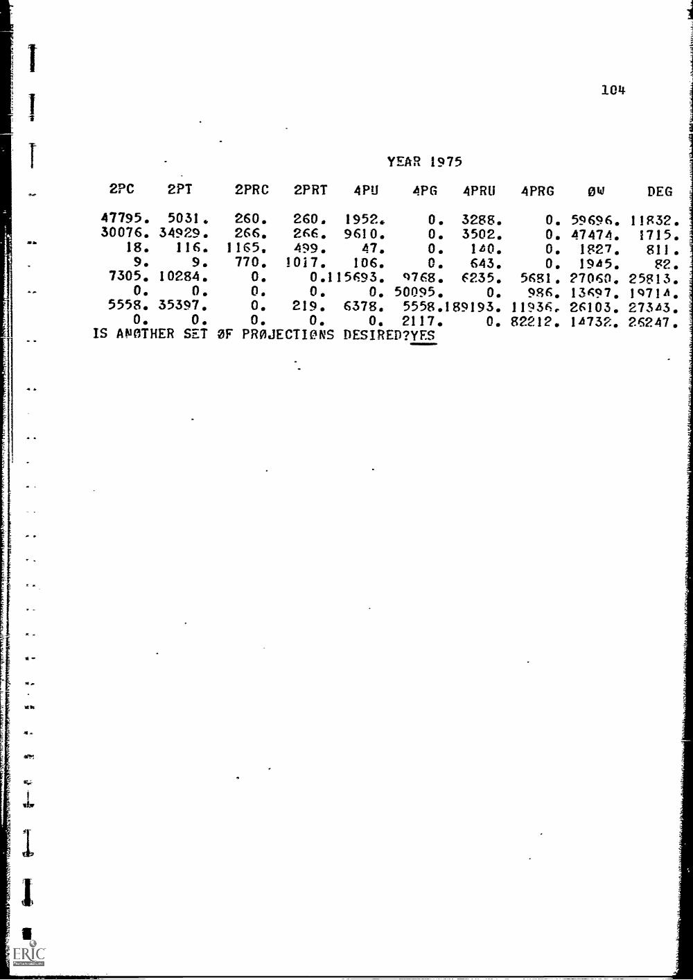
104

2PC 2PT 2PRC 2PRT 4PU

YEAR 1975

4PG 4PRU 4PRG OW DEG

47795. 5031. 260. 260, 1952. O. 3288. O. 59696. 11832.30076. 34929. 266. 266. 9610. O. 3502. O. 47474, 1715.

18. 116. 1165. 499. 47. O. 140, 0, 1827. 811.9. 9. 770. 1017. 106. 0, 643, O. 1945. 82.

7305. 10284. O. 0.115693. 4768. 6235. 5681, 27060. 25813.0, 0. O. O. 0. 50095. O. 986. 13697, 1471A,

5558. 35397. O. 219. 6378. 5558.189193. 11936r 26103. 273A3.O. 0. 0. O. O. 2117. O. 82212. 14732. 26247.

IS ANOTHER SET OF PROJECTIMS DESIRED?YES

105

SECTION III

CASE STUDIES

A. Introduction

The case studies reported in this section

represent an attempt to implement the simulation model

in three different yet collectively representative

educational systems. Consequently, these studies represent

a set of real world experiments designed to assess both

the conceptual validity and operational feasibility of

utilizing the simulation model for planning purposes. The

purposes of these cases were then twofold: (1) to

assess the relationships between the existing higher

education data bases and the input requirements of

the simulation model; and (2) to evaluate the usefulness

of the prototype model to educational planners at the

institution level. A major concern of the data

requirements was with the potential disparity between the

content, disaggregation, accuracy, reliability, and level

of precision of the information required and that found

in representative sources.

Two alternative (but not entirely mutually

exclusive) procedures for amassing the required input

information were attempted:

1. asking for subjective estimates from

knowledgeable persons at institutions

of higher learning and combining these

106

estimates with existing aggregate data;

and

2. statistically sampling unit records at

representative institutions.

The four institutions chosen for this initial

experiment compose a representative cross-section of the

higher education system in New York State.

The City University of New York (CUNY) is a

tuition free institution which offers approved graduate

and undergraduate programs in nine four year senior

colleges and six two year community colleges in New

York City. 1967 enrollment has expanded to 144,000

students, of which 64,000 have been full-time, matri-

culated students.

Rensselaer Polytechnic Institute (RPI) is a

private non-sectarian, technological university in Troy,

New York. Rensselaer emphasizes a technological

education in Engineering and Science on both the under-

graduate and graduate levels. Architecture, Humanities

and Social Sciences, and Management curricula are also

offered on the same levels. At the present time,

Rensselaer has a coeducational environment of approximately

3,550 undergraduate and 1,100 graduate students.

Hudson Valley Community College (HVCC) is one

of thirty-one two-year community colleges locally

107

sponsored under the program of the State University of

New York. It has a current enrollment of 3,833 full time

students at its campus in Troy, New York. Most of the

students are distributed among six academic divisions

wIL.L.t.a1

Syracuse University in Syracuse, New York is

a semi-private educational institution with a total

student enrollment of nearly 23,000 in the Spring of

1968. Syracuse has 15 undergraduate schools which

include the State University College of Forestry and

Utica College in Utica, New York. The graduate school

offers advanced studies in all undergraduate areas as

well as in architecture and social work.

In the case studies to follow, the above

alternative procedures will be seen to have been

implemented in distinct but complementary ways. By

far the greatest amount of effort was devoted to the

evaluation of the CUNY data base: it was felt that

not only would CUNY yield many difficult problems

relating to data acquisition for the prototype, but that

it was, as a system of colleges, an analogue to the

statewide educational system. With the latter thought

in mind, it was decided to evaluate both methods 1 and

2 above at CUNY, although, as will be noted, actual

unit record collection was not performed as a result

of this evaluation.

108

At Rensselaer Polytechnic Institute a data set

fulfilling the requirements of the prototype was collected

through the sampling of individual student records. Sub-

jective estimates of knowledgeable individuals were com-

bined with aggregate data on file in the registrar's

office for the development of a data set at Hudson Valley

Community College.

While not mentioned in the cases, an advanced

management information system in use at Syracuse University

was studied to determine whether the form and content of

the data which could be retrieved would meet the input needs

of the prototype. The study showed that the information form

and content of this system while quite advanced were not

amenable to analysis by the simulation model. As a result,

Syracuse University was not included as a formal case study.

The selection of the above institutions as

representative was made with several practical considera-

tions in mind, including the minimization of travelling and

living expenses associated with the research activities and

the administrative cooperation necessary before the data

collection could be carried out. Thus, Rensselaer was

chosen as the institution at which to conduct the unit

record sampling since it was known that such a process

would be time consuming and much in the way of travelling

and living expenses could be eliminated. Selection of a

small college for the collection of subjective estimates

as

a a

a

109

would enhance the probability that they could be obtained

in the quantities required and time available. Hudson

Valley Community College proved to be eminently suitable

for our purposes.

Syracuse University had been considered for

study of the electronic data processing information

system in collecting and storing data as it was commonly

felt to have the most highly automated system. It may

thus be seen that the initial sample of schools felt to

be "representative" involved a large public university

system, CUNY; a large private school, Syracuse University;

a small private 4 year school, Rensselaer Polytechnic

Institute; and a small public school, Hudson Valley

Community College.

The ensuing part of this section involves

three cases; those of CUNY, RPI, and HVCC, in that

order. Following the three case discussions, conclusions

on viable approaches to data accumulation for the proto-

type will be drawn with an eye toward information content

desired, and data availability and form.

B. Case Study: City University of New York

The City University of New York was formed in

1961 from the autonomous colleges previously associated

through the municipal college system. Student data

systems at these colleges were as different as the schools

themselves at that time. These long standing information

systems remained unchanged wiLh the consolidation into

_a

110

the City University. Since that time, some movement has

been made toward a more uniform data set, and recent

developments have seen the schools agreeing on some common

definitions of academic level and status classifications,

although all historical data are locked into the

previously established categories.

The forces affecting enrollments of the City

University of New York offer great substance for a

simulation model and great opportunity for its use.

The policy of the City University is to offer regular

admission to qualified residents of New York City and

special admissions from approved programs to a number of

disadvantaged graduates of City high schools. The

university is tuition free and relies heavily on the

City and State for support. CUMY is composed of nine four

year senior colleges, and six two year community colleges.

Student transfers, both between the two types of

colleges and among colleges of the same respective type

are frequent. The university is in a period of expansion,

especially in its community colleges and special programs.

While each college maintains a degree of autonomy in

determining its own destination, university wide policies

W W are set by the Board of Higher Education. The Dean of

the Master Plan is responsible for anticipating and

planning for university growth.

111

The areas of model building explored and

evaluated at CUNY include:

1. determination of major classification scheme

and categories of characteristics;

2. methods of determining required parameter

values;

3. methods of updating the historical data

as new yearly sets become available, and

of collecting the new sets;

4. implementation of special user features,

such as real-time remote access to the

model program, and allowance for changes

in projected data according to subjective

estimates.

For clarity of presentation, this section is

divided into two major parts: the first deals with the

potential of using individualized records to

provide input to the simulation, and the second deals

with a model whose results are a function of the

aggregate data collected for it.

1. Feasibility of Unit Record Data

As previously discussed (and inherent in the

structure of the model) the specific content (the

classifications and characteristics into which students

are grouped) are specified by users. To help determine

the form of the desired output information, a preliminary

112

meeting was held at the New York City Board of Higher

ECucation Building on July 11, 1968, and attended by

State officials, CUNY planners, representatives from

the CUNY council of Registrars, and members of Rensselaer

Research Corporation. Since this portion of the study

would involve the examination of the permanent record

systems of all schools within the CUNY system, this

meeting also served to insure uniform prior knowledge

and cooperation among all those concerned.

Problems were encountered in determining the

content of the desired output. One difficulty arose

primarily from the CUNY participants' initial lack of

acquaintenance with the Aodells workings, in particular,

its dependence upon historical data as the basis of

projections. Output information objectives initially

proposed by the university administrators and registrars

were diverse. Many of the classification criteria

suggested were not appropriate to this simulation or

would not be present in any historical data. In short,

many of the suggested objectives could not possibly have

been met. The sum total of the "desired output" was

actually a university wide data system. It was concluded

that current projection objectives would be restricted

to those classifications covered historically by the

presently existing information system.

113

The CUNY information objectives are shown in

Figure 9. Students were to be aged through the CUNY

system according to their specific college and level at

respective points in time. With nine senior college day

programs, seven senior college night divisions, six

community college transfers programs, and six community

college career programs at distinct colleges (that is 28

"colleges" in all) and four levels for the senior colleges,

with two levels for the community colleges, the total

number of components in the major classification scheme

would be 88. There would be six characteristics used

as students descriptors: ethnic factor, student course

load per semester, high school average at entrance,

sex, status, and source of entrance to the CUNY system.

For these six characteristics, there would be a total

of 24 categories describing the students. In order to

fulfill these information requirements, the set of data

required from each student record would be that given

in Figure 10.

Since unit record sampling needed to be carried

out at all colleges, and since the model could incorporate

only those groupings about which information could be

gathered at all colleges, it was necessary to examine

the file organization and permanent record form content

at each school.

114

1. Major Classification SchemeFreshman

9 Senior Day Colleges SophomoreJunior

7 Senior Evening Colleges Senior;

6 Community Colleges Career ProgramsFreshman

6 Community Colleges - Transfer SophomorePrograms

2. Characteristics & Categories Within

Sex - M-F

High-School Average - 100-90,90-82,82-75,75-0

Ethnic Factor - Negro, Puerto Rican, Other

Source of Entrance - Regular NYC H.S. Senior,College Discovew, SEEK,Advance Standing fromoutside CUNY, other.

Course load/ semester(units) - 2-4,5-7,8-10,11-13,14-16,17+

Status - Matriculated; Non-matriculated,Inactive honorable,inactive dishonorable

FIGURE 9

INFORMATION OBJECTIVES OF A CUNY MODEL

(See Figure 2 page 21)

115

1.

2.

Present Level

College Profile

Freshman, SophomoreJunior, Senior, Graduated

College attended atbeginning and end of eachrespective level, (Day-Eve.for Sr. Colleges andCareer-Transfer for CommunityColleges treated asseparate schools)

3. Credits Complete to Date Exact Number

4. Ethnic Factor Negro, Puerto Rican, Other

5. High School Average 100-93, 89-82, 81-75, 74-0

6. Sex Male, Female

7. Year of Exit Last two digits of year.

8. Degrees Received in System Associate, Bachelor

9. Type Admission to CUNY System Regular, NYC High SchoolSenior, College Discovery,SEEK, Advance Standingfrom outside CUNY, other.

10. Level of Entrance Freshman, Sophomore,Junior, Senior

11. Year of Entrance Last two digits

12. Entering Status Matriculated, Non-matriculated

FIGURE 10

INDIVIDUAL STUDENT DATA REQUIRED

ry

In sampling records of various years,

representative records must be chosen from the files at

hand. Consequently, organization of the registrars file

systems largely determines the applicability of any

sampling plan.

Furthermore, this data must be available from

all colleges of the university system. Content of

permanent record forms at CUNY, however, varies from

school to school. The university does not have a homo-

geneous student information system. Differing information

codes must be interpreted before the products of the

different data systems can be combined into a single

data base; and there is difficulty at CUNY in this

respect due to the lack of common definitions of such

terms as "sophomore" and "full-time" as well as the

variations in form of data presentation on the records.

Registrars and assistant registrars from all

institutions within the CUNY system were interviewed,

and all record systems examined. The distinguishing

features of the respective information systems were

noted; and their effects on the intended sampling were

anticipated. Since it was felt that difficulty

might be encountered in obtaining certain narrowly defined

cross classifications of students, the registrars were

asked whether they would be able to supply us with "reasonable

estimates" of these cross-classifications. Only in certain

cases were the registrars querried able to provide this

information.

117

A sampling plan was not devised in the case of

the CUNY evaluative effort. Study of the individual data

files of the separate institutions within CUNY indicated

that there were great differences in the manner of reporting,

as well as in the actual information reported on them.

In addition, the organization of the files themselves

were very different from institution to institution.

For example, some information systems' records are split

into two sections: active and inactive, and arranged

alphabetically. On the other hand a record set might

be divided into four active files, and five inactive

files, with such titles as "bachelor dropouts", "associate

dropouts", "non-matriculant dropouts", and so forth, some

of which are arranged by date of admission or inactivation.

Some of these schools are in periods of transition of

their data files or have very recently completed such a

change period. The resultant file variation over time would

necessitate different plans for the sampling of different

years' data even within a single school. Finally, York

and Richmond Colleges, the youngest of the senior colleges,

have file organizations lending themselves quite well

to sampling; but by virtue of their newness, they have

only one year of records which could be sampled.

Assuming that a working sampling plan could

have been constructed to deal with the various file

arrangements, the feasibility of data collection would

118.,a

have depended upon how well the data requirements stated

in Figure 10 were met in the student record forms.

Certain problems arose in this sphere. Thus, for example,

ethnic factor is not available from any school's record

form. The ethnic census of the university taken in

September, 1967, provides only one year of data. In

addition, its results were divided into the classifications

of school and level but not into the more detailed sets

described by the intersections of these categories such

as School 3, junior level. Another factor difficult to

obtain in general was that of high school average.

Particularizing, the record form of Staten

Island Community College does not furnish a day-evening

distinction. Other community colleges fail to differen-

tiate between career and transfer programs students on

their records. Some colleges do not distinguish between

students admitted through the special programs, SEEK and

College Discovery. Another important factor concerning

incoming students is their previous college work; though

such information is critical in the development of flow

parameters (transition proportions), not all schools

specify colleges of transferees' prior attendance.

fir

119

2. CUNY: A Pilot Model Based on Aggregate Data andSubjective Estimates

A primary goal for the effort at City University

was to implement the prototype model for CUNY's use based on

parameters whose values could be developed within reasonable

time and with data currently available. While individualized

sampling was found infeasible, the central Office of

Institutional Research (OIR) offered another approach to

initial data collection. Aggregate enrollment and

admissions figures are reported by the CUNY colleges to

this office. While this form of data necessitated

modification of original information objectives, these

changes did not detract from the model's usefulness as a

planning tool constructed for direct use by administrators.

Development of the data set was monitored and guided by

T. Edward Hollander, Dean of the CUNY Master Plan.

Based upon broadly defined informational needs of the

university planning function a feasible set of data

requirements for the model was established. Similar to

the individual colleges, the University OIR has varied

its data collection forms considerably over time. An

effective likeness among yearly enrollment, admission,

and attrition reports goes back only to the 1965-1966

academic year. Therefore, only these "compatible" data

were collected, and the prototype for CUNY projects on the

basis of three years' historical data -- 1965, 1966, and

1967.

120

The present emphasis of the planning in the City

University is on the period ending in 1975. In its

1964 Master Plan, CUNY states a recently adopted goal of

implementing a 100% admission policy by 1975 through

expansion of programs at the senior and community colleges.

According to this goal, the University will be able to

offer some form of higher educational opportunity to all

graduates of New York City High Schools. It must

anticipate student demand, outside influences, and its

own potential outlets for growth via expansion as well

as new programs. Therefore, the study focused on the

1968-75 period,

In offering admission to a less and less compe-

titive group of students, CUNY will try to channel a

disproportionately large segment of the enrollment increment

to its two-year community colleges. After graduating from

one of the latter a student is guaranteed of junior level

admission to the senior college of his choice. It is

felt that this policy will provide a framework wherein

the most talented and motivated students can go on

through a fouryear college experience while all high

school graduates regardless of prior achievement are

afforded the opportunity of doing some further work. The

university administration is basically concerned with its

community colleges, senior colleges, levels of academic

attainment, and special programs as whole units.

121

The revised classification scheme chosen to best

suit these concerns involves six components: community

colleges as a group with two levels within them, and senior

colleges as a group with four levels within them as

shown in Figure 11

community college

senior college

Figure 11

[

freshmen

senior

(freshman

sophomore

iunior

senior

THE CUNY MAJOR CLASSIFICATION SCHEME

The associated form of the transition matrices

for the CUNY model is shown in Figure 12.

Growth will heighten CUNY's problems of keeping

aware of the representations of certain groups in each

of the University's constituent parts. Although the 1967

ethnic census shows that CUNY has the largest minority

group enrollment of any institution in the country, the

percentage representations still do not reflect the

ethnic distribution of the City's high school graduates.

New programs to be initiated shortly will change the

119

__...............

'.....

Community

Colleges

1,0.

31

Senior Colleges

Fr.

So.

Fr.

So.

Jr.

Sr.

ATT

Grad,

Community

Colleges

N0

F.

all

a12

a13

a14

a15

ale

a17

a18

So.

a21

a22

a23

a24

a25

a26

a27

aig.

Senior

Colleges

Fr.

..

..

..

pm a

mus

ft

.

--,......

.

So.

.

.....

..

..

Jr.

..

..

..

..

Sr.

a61

a69

a63

a64

a65

a66

a67

a68

FIGURE 12

EXAMPLE OF A TRANSITION

MATRIX FOR THE CUNY

MODEL

123

University's ethnic mix. To gain insights into the effects

of such ptsograms it was decided to include ethnic

classification as a student descriptor.

Also of interest are enrollment breakdowns by

"means of entrance" to CUNY. Students may be admitted

from regular NYC high schools, out of Neer York City or New

York State, the special programs (SEEK and College

Discovery), or the "outside world," including transfers

from the evening division and private colleges. Source

of entrance, then, was chosen as a second student

descriptor or Characteristic.

All data outputs are based on the enrollment of

full-time day session matriculants and special program

students. With the model specifications formed to

reflect these conditions and the ones discussed above,

the necessary data could then be gathered.

In modeling student flows at CUNY, total

students, first-time freshmen, and upper-level entrants

were vectors rather than matrices of students. A vector

of total students was cycled through a transition

matrix, vectors of first-time freshmen aad upper-level

entrants were added to the result, and eac element in

this new vector of total students was multilpied by a

vector of percentages which allocated the students among

the categories of Characteristics. In the newer forms

of the model, it might be said that this apportionment

124

is carried out for the first-time freshmen and upper-

level entrants separately and before cycling through a

transition matrix.

As might be expected, the historical data

required for each year upon which the projections would

be based were as follows:

(1) vector of first-time freshmen grouped

by the major classification scheme;

(2) vector of upper-level entrants grouped

by the major classification scheme;

(3) for each component of the major classifi-

cation scheme, a vector of percentages

describing the apportionment of students

among the categories of characteristics

being used as student descriptors.

In addition, for the first historical year, a vector of

total students grouped by the major classification

scheme and corresponding to the "starter" matrix of the

present form of the model would be required. Analogously

with the starter matrix, the starter vector would involve

total "head-count" of students in the appropriate year.

In that which follows reference to the vectors of

percentages describing the apportionment of the students

among the categories of descriptive characteristics is made

in terms of "Output Breakdown Vectors (OBV)" and the matrix

formed by all OBV for agiven year is called an output

breakdown probability matrix (OBPM). As will be recalled,

125

the need for such vectors or matrices in the newer versions

of the model is limited to those characteristics which vary

in some irregular manner over time.

Of the five facets to the data set necessary for

implementation of the prototype, the starter vector,

vectors of first-time freshmen, and vectors of specifically

defined student totals are taken directly from aggregated

historical records. The transition proportions, however,

are not available in the records, and must be developed

from ocher available information.

The proportions in each year's OBPM, qij, (Sec

Figure 13) can be obtained by dividing the number of

classification i students in category j by the total

number of classification i students. For example, q32,

the likelihood that any Senior College freshman is Puerto

Rican, is equal to the number of Puerto Ricans in the

senior-college freshman class divided by the number of

all Senior College freshmen. Only one year of historical

data, 1967, was available to describe ethnic distribution.

Subjective estimates of yearly percentage changes in ethnic

distribution over the years dating back to CUNY"s prior

Master Plan (1964) were applied in reverse, starting from

the 1967 figures, to find the "data" for 1965 and 1966.

Values from which to obtain the source of entrance probability

elements were taken directly from the aggregated enrollment

and admissions forms.

Level

Comm. Coll.

Frosh (1)

Comm. Coll.

Soph (2)

Sen. Coll.

Frosh (3)

Sen. Coll.

Soph.

(4)

Sen. Coll.

Jun.

(5)

Sen. Coil.

Sen.

(6)

Ma1

"ral

.1.!

r"T

rn4

Ethnic

Negro (J.)

Puerto Rican (2)

q11

q12

q21

q22

q31

q32

q41

q42

q51

q52

461

q62

Other (3)

Regular

N.Y.C. H.S1111)

Out of

City (5)

Source

Out of

Outside

State (6)

World(7)SEELU8

College

Discovery (9)

q13

q14

q15

q16

q17

qlb

q19

q23

q24

q25

q26

427

q28

q29

q33

q34

X35

q36

q37

q38

q39

q43

q44

q45

q46

q47

q48

449

q53

q54

q55

q56

q57

q58

q59

q63

q64

q65

q66

q67

q68

q69

FIGURE 13

GENERALIZED OUTPUT BREAKDOWN PROBABILITY MATRIX (0100

127

While, again, much of the required data could

be taken directly from aggregated historical records,

the transition proportions were not available in the

records and had to be estimated on other bases. The

component probabilities of a transition matrix are

proportional to the yearly movements of students from

positions within the system to other positions within or

outside it By the nature of an educational system some

of these probabilities are very close to zero, for a

senior college junior will ordinarily not become a sopho-

more or a freshman, a freshman generally will not become a

junior or senior by his next year, and so on. Therefore,

before trying to evaluate any of the probabilities, it is

necessary to look at their meanings in the context of

the real CUNY system.

Figures 14 and 15 diagram student flow through

the real CUNY system in notation as defined in those figures.

The diagrams show all inputs to and outputs from each

classification in the system. In Figure 14 Regular (Reg)

and College Discovery (CD) inputs to the freshman class (F)

make up the level #1 element of the T vector (vector of

first-time freshmen). The input of year (k-1) freshman to

the freshman class of year (k) represents the portion of

year (k-1) freshmen who stay back to remain freshmen in year

(k); as a percentage of all (k-1) freshmen, this flow is

equivalent to all in the transition matrix (AMX). Similarly,

the input of year (k-1) sophomores to the sophomore class of

year Oa determines a22, and the flow of stayback freshmen

128

for the year k, gives all of the kth year transition matrix.

There is flow between the system and the Outside World

(4W) from all classifications. Record forms state the

flow from the outside world to CUNY only in terms of one

component to Community Colleges (CC) and one to Senior

Colleges (SC). Assumptions were made that permitted these

two components to be split into flows to each of the six

respective levels; the Community College component is split

evenly between freshmen and sophomores, while the Senior

College component is divided into 20% freshmen, 60% sopho-

mores, 20% juniors, and no seniors. (Notice that there

are no input arrows to Senior Level from the Outside World

in Figure 15.). Flows from CUNY to outside world occur

at all levels. These attrition totals are given in aggregated

attrition reports by year and classification. Dividing

the year k absolute flow values by the total enrollment

in the corresponding classification yields the ate, i =

1,...,6 of the year k transition matrix. In Figure 14,

there are seen to be two-way yearly flows of students

between Senior College and. both levels of Community

College. Figure 15 shows these flows from Senior College

perspective, The set of specific level-to-level inter-

college transfers existing in CUNY was outlined by planning

officials at CUNY. All Senior College flows to Community

College freshmen level originate from the freshmen class of

Senior College; thus, a31 represents this flow and ala= a6l="

All Senior College flows to Community College sophomore

class and are therefore represented by a42, while a32=a

52=a

62=0.

Notation Key, Figures 14 and

15

Reg - regular first-time

freshmen

CD - new College

Discovery

program freshmen

F - freshman class

S - sophomore class

OW - outside world

SC - senior colleges

G - graduates to

outside the

system

SEEK - new SEEK program

freshmen

J - junior class

SR - senior class

FIGURE 14

STUDENT FLOW - COMMUNITY

COLLEGES

RegSEEK)OCY

kOST

k

CCRegok+1

SEEKI0.1OCYk+1OST

k+1

OW

CC

Sk

CC

t

130

I

Fk+1

ow

CC

OW

OW

SRk

OW

OW

_LNOW G

FIGURE 15

STUDENT FLOW - SENIOR COLLEGES

SR

3/

OW G

131

Transfers are allowed for qualified Community College

freshmen to Senior College. All of these flows go to the

sophomore level and correspond to a14, so that a13=0. From

the sophomore level, Community College students may

graduate and go on to junior level studies in Senior

College (a25); they may also transfer without graduating,

in which case they go to the sophomore level (a24). Besides

transferring, staying back, and dropping or being cast off

to outside world, the only other output from the Community

College sophomore class is through graduation to outside

the system (a27). Therefore a21=a23=a25=0. Figure 15

shows the components of the third element of T to the

Regular, SEEK, Out of City and Out of State. Finally, it

is seen that the lines of "normal" progress through the

system are represented by Fk to Sk41 Sk to Jk4.1, and Jk

to Srk+1,the probabilities associated with these flows

being a12 for Community Colleges and a34 a45, and a55 for

Senior Colleges. Of course, a student may either remain at

his level or progress to a higher level after a year, but

he generally will not make negative progress. Therefore,

a21=a41

=a51=a61

=a52

=a62

=a23=a

43=a53

=a63=a54

=a64=a65

=0.

Finding values for all a.. in a transition matrix

amounts to quantifying the flows represented by all output

arrows from year k levels. It is seen that many of these

are riot feasible transitions and hence many flows are zero.

Some others are directly defined or easily calculable (given

subjective estimates) from enrollment, admissions, and

attrition reports. The only flows that are not available

132

here are those of "staybacks" (i.e.: all, a22,etc.) and

those of normal progressions (i.e.: a12 a341 a452 a56)

through a college. They are represented by the horizontal

and diagonal (pointing towards lower right) arrows of

Figure 14 and 15. All other inputs and outputs are

essentially known. Notice that if just one of the unknowns

is found, the others (in that particular year) are

automatically determined. That is, if the senior college

Fk to Fk+1flow is found, it can be added to the Fk

transfer and outside world flows (which are known) to

obtain a quantity which when subtracted from Fk yields as

a difference the only remaining output flog, Fk to Sk+1.

In terms of transition probabilities,

8

a3j3=1

1,

that is, the row sums must equal 1, but as shown above,

a32=a3536=a38=°'

therefore, a31+a33+a34+a37=1;

and letting the known sum, a 31+ a

37= C,

a34

= 1-C-a33,

so that knowing a33, the freshman stayback rate, is

equivalent to knowing a341 the freshman to sophomore flow

rate. Since all inputs to Sic+, are known previously

except for the Fk to Sk and Sk to Sk flows, this newly

computed parameter, a34, by determining Fk, to Sk also

determines the sophomire stayback rate, awl, from year k.

The rest of the unknowns are calculated by this simple

difference technique in the light of the facts that

133

e

S a.. = 1 and the sum of the inputs to a level must equalj=1 13

that level's total enrolltent. Since the unknowns are

interdependent, the problem is reduced to that of

finding just one of file unknown flow rates. The

solution is seen in looking at the inputs to F; they

include T (which is given), E (which is given), and

staybacks from the previous year. Symbolically, then,

for any year k,if V3k represents the total number of

classification 3,

V3-T

3-E

3a33 V

3(k-1)

where V3(k_l) is senior college freshman enrollment of

the previous year.

In the model, first-time freshman vectors

(T) are projected from the corresponding vectors in the

historical data. Freshman admissions at CUNY, however,

are a function solely of space available. Knowing the

distribution of New York City high school seniors'

academic averages, planners simply draw the cutoff line

at a percentage selected to give the desired number of

acceptances and henne expected admissions. In fact, the

CUNY administration can plan on yearly admissions

goals and then see that they are met by drawing the

appropriate cutoff line each year. The 1968 Master Plan

states explicitly what first-time freshmen admissions

r.

1.

1

134

to senior and community colleges should be for the years

through 1975. It is therefore not the CUNY model's task

to project them, but to accept these Ti, i = 1968,...,

1975, as known input to the model. The model was

appropriately (and easily) modified to do so.

A change of form was made shortly thereafter.

The transition matrix contains aiik's to reflect

average behavior; by the very nature of these

probability elements; but it is known that performance

of. Special Programs students (those admitted through

SEEK and College Discovery) differs from that of the

" regular" matriculants. Although the SEEK and College

Discovery students have historically made up a very

small portion of total enrollment, growth of these

programs as well as inception of new ones adopted in

August, 1968 will boost the total enrollment through

special programs (SP) to increasingly significant levels

up through 1975. It was therefore decided to flow the

special programs population through a transition matrix

of its own developed from historical records of SEEK

and College Discovery students.

Upon adoption of the new programs CUNY

planners were at once faced with the problem of

judging their effects on total enrollment and ethnic

distribution of all students. To isolate these effects

the CUNY model was programmed to handle different

data sets, one concerning all regular full-time day

135

matriculants and the other concerning students in SEEK,

College Discovery, and the new special programs. Trays

represents an application of the model's ability to

respond to contingency questions, for in adding the new

educational programs to the model, planners were

essentially asking "What would be the short and long run

effects on the system if (a) new program(s) were added?"

In terms of data requirements they needed only supply

yearly T vectors for the new program(s) since T for SEEK

and College Discovery were already known, all special

program students enter as Freshmen (E=0), historical

V's for SEEK and College Discovery were known and for

new programs were equal to zero, the transition matrix

had been already calculated, and the OBPM's were

available through Dean Hollander's office. The T vectors

were given by the CUNY administration on the basis of the

construction of the new programs. To the original program,

the split meant having only to subtract SEEK and College

Discovery of all T vectors and to recalculate a shortened

OBV without the SEEK and College Discovery elements. The

Special Program data set was expanded to include the data

of the new special programs within each set representing

a different combination of special programs whose effects

were to be examined. Since this amounted to subjecting

the simulated system to six different possible sets of

forces, the Special Program section is termed the

"Contingency Model"; the other section, having only one

Ft FA

ire

136

data set, is the "Constant Model," though this name is not

meant to imply that contingencies cannot be tested on it.

Planners can ask questions of either model by changing

the appropriate data inputs: a subsequent run would show

the system's response.

Since the nature of the planning process demands

that many contingencies be tested under several assumptions

the model was adapted to a real-time computing system

the model was put "on-line". Program changes and the

addition of English language statements to ease

communication made for the following specific user features

in the on-line model:

(i) Selection of Output Displayed. The user

need not receive the entire model output if he is

interested in only specific parts of it. He may order

that any combination of any number of the parts (AMX,T,E,V,

OBV) be printed (for specific projected years in the cases

of AMX and OBV).

(ii) Dictation of Number of Projected Years.

Although because of core limits the model is set up to

project only eight years (1968 through 1975), the user

may not be immediately interested in all cf them. He

can input at a run's outset the number of projected

years to be included in printout.

(iii) Ability to Change Projected Values. A

planner might have reason to believe that the trend

implied by projected values does not agree with his

educated intuition. If so, he can change any projected

137

value(s) that differ from his expectation. Any change

thus made also affects other projected values. The

user may choose either of two ways in which this

influence is manifested: through the "dynamic" or the

"episodic" update, as discussed in Section II of the

report.

3. CUNY: Evaluation and Conclusions

The CUNY simulation model was set up not only

as a direct aid to City University planners but also

as a prototype from which to develop a systematic

approach adapting the general model to a specific

educational system, and measuring the effectiveness of

its methodology in that system. After specifications

to orient the model's output to particular planning needs

were set, a general technology was introduced for

development of initialization data from yearly aggregate

reports. Evaluation of the devised application

techniques was made with respect to the original

objectives of the simulator. Th two general areas of

focus were:

1. accuracy of the projections, and

2. usefulness of the simulation's ability to

react to contingencies.

Since the CUNY model projections are made on

the basis of three data points, any irregularity in a

data point from a given year has significant effect on

138

the projected value of a variable. Projection from a

greater number of observations reduces the potential

impact of such irregularity. It is to be expected, then,

that additional years of data collection at CUNY will

bring more reliable projections.

A second area of evaluation reflects the

accuracy with which the model represents the CUNY

educational system. The greatest value of any simulation

model is in its capacity to help the planner contemplate

"what-if" questions. It is in this capacity that the

CUNY model has proved most-useful; the latter helped

to identify both short and long range effects of the

additional special programs considered by the university

administration. When the model was put on a real-time

basis, the system was tested "on-line" for sensitivity

to several hypothetical policy decisions. One such

"decision" dictated the admission of five hundred

additional special programs freshmen in 1970. The

immediate output response showed the expected distribution

of these students in years 1970-1975. Thus, CUNY

planners could judge incremental effects of this one

event on particular system components in the long run.

The speed of the time-sharing output was found to be

as important as the resultant figures themselves. It

is often the case that City University planners wish

to find the causal action required to produce a desired

effect on enrollments. The real-time-system enables

a

139

them to "try' various actions in succession to deduce a

most suitable policy.

Model uses presently being considered include

applications to university budgeting and yearly revisions

of the Master Plan. The development of a university-

wide information system will greatly increase the potential

for such a simulation while at the same time it will

enlarge the awareness of the utility of the model as part

of an expanding planning medium.

C. Rensselaer: Unit Record Sampling

The implementation of the prototype model at

CUNY provided experience in initializing the planning

model in the context of a large educational system.

As we have seen this system had many diverse data sources,

but the structure of the student information both within

and between these individual sources did not lend

itself to easy and rapid initialization of the simulation.

On the contrary, preparing the simulation for use at

CUNY required an amalgam of methods for gathering the

requisite data. The ability to draw data from an

homogeneous data system could potentially have alleviated

many of the problems associated with the CUNY study.

Rensselaer Polytechnic Institute was chosen

as a representative institution within which the

planning model could be utilized by providing input

data from a sample of unit records. In addition, a

140

parallel attempt was undertaken to utilize subjective

estimates of the academic deans at Rensselaer as an

independent measure of student flows in order to provide

a measure of validity to both the input and output (of

the simulation) generated by sampling unit records.

This attempt at validating the simulation by using an

independent set of data inputs proved impractical. None

of the academic deans felt qualified in providing accurate

flows either within their school or between the five

separate schools of Rensselaer. Although the registrar

might be able to provide such estimates, the level of

disaggregation required by the model at Rensselaer

precluded the possibility that the registrar's office

could provide data on the precision desired while main-

taining an independence from the students' unit records.

Consequently, the study at Rensselaer concentrated on a

sampling of unit records augmented by several aggregate

reports previously prepared by the registrar's office.

The initial phase of the unit record sampling

study helped determine the form and content of the unit

record data and involved a detailed investigation of

the educational structure in order to obtain historic

knowledge of student characteristics and "aging"

processes.

The preliminary study of the availability of

data set the ground work for the development of the

sampling form. This sampling form was structured so

141

as not to confine the sampler to any one sampling

design.

The sampling form involves a row tabulation of

information from individual student personal record

cards (PRC forms). From the information extracted

separately from each sampled student's PRC, a historic

trace of his aging process is recorded on the sampling

form in terms of the classifications and charactsristics

delineated by the model (see Figure 16).

The "class profile" is the record in which

each student's historic movement through the educational

system is recorded. Corresponding to each level, the

appropriate curriculum can be recorded fa:, each student.

Space is alloted for two years at each level (where the

second year is for a repetition of the level). The

other information is required for categorization of

each student, for the location of his entrance and exist

from the system, and for credit hour distributions.

The class profile of all students can be added up to

give empirical transition frequencies. By dividing

through by the row sum for any matrix of frequencies,

the transition probabilities are calculated.

1. File Organization

A brief description of the file organization

at Rensselaer is presented to provide an understanding

of the difficulties of randomly sampling student PRC

142

FaiihingtEntecing

04.

Lew21i mw

i

w1-f',A

(IAo5:1

o,-1

w1.,It0

<4.t

i

Graduate

I

G2

ii6

G1

.,

Pi)

I.nin

Fifth YearFY

2it

1.1.1

1

T et

lin ,

SeniorSE

2

0m,-N,

SEb"..

ri

JuniorJ2

v''0

f ri

J1 fl 4Iofrt

SophomoreS2

4 iI-K I

1 13'*4

1 4

F2

I L':

.

N,FreshmanF1

vIZ1 .

GeographicOrigin

i

, z

,..

AgeI ".

,

1

.

Sex I o IYear of Entry

1K

ut.

IdentificationNumber

v.._

>,

fn

1

1,ri

II

FIGURE 16

R.P.I. UNIT DATA COLLECTION FORM

F

1

143

.10

1111

rd0

,_3

5.

ox4-1

10i-ifd

Graduate

G5 WIIII

4T11111111111111

go.

1011111111111111. OMili

MOMtailfi

IMMMOMI S

1 11a

Fifth YearFy2

111

%.'

$

SeniorsE2

h

SE

III..4

1Juniora1/4

Sophomore'b2

i

1III .

Freshman

, 11MIRl NNE

IMIIIMUKIIIIM

11

11111CO

0) a)w 054 .14b0

Doct.Year 1S

YearI I

Nast. ,011311

'il in1111

Year11co 4J

A Ao Bach. i_ti

, IIISchool . I

FIGURE 16 (CONTINUED)

144

forms. The arrangement of the PRC forms contributes not

only to the difficulty or ease of sampling, but also

helps to determine the sampling design.

Inactive students or those who have already

graduated or dropped from school are filed as a group

in alphabetical order. All active full-time graduate

students are also filed together by the order of the

alphabet. Part-time graduate students are grouped in

the same fashion. Finally, the graduated students of

the past year (in this case 1968) have been placed in

a separate file by order of the alphabet. A compounding

problem arises here because undergraduate and graduate

records of students who have matriculated in both the

undergraduate and graduate degree programs are placed

on two different PRC forms, A student who has completed

an undergraduate degree program and is now an active

graduate student or has received a second or third

degree in the past year would have one inactive PRC

form and one either active PRC form or graduate PRC

form, depending on his situation. Fortunately, the PRC

forms are cross referenced so that each student's entire

record can be sampled. It should be stressed here than

when a student is chosen for the sample (the choice

being dependent on the design of the sample), the entire

profile of a student while in attendance at Rensselaer

is sampled. The reasoning is that the summations of

characteristics and transitions of individuals who "age"

145

over their matriculation at Rensselaer is the procedure

by which the computer model transforms individualized

data into transition probabilities and matrices of

entering students. An alternate procedure consists of

sampling students for only a particular transition, for

example junior-senior transitions. Such a procedure

may be equally as valid and could be conducted with less

expenditure of effort depending on the file organization

at the institution being studied

The set of data required by the sampling form

can be generated from the individual stmlents' PRC

form. Other information had to be collected for the

initialization of the model, but was dependent upon

the sampling design.

2. A Sampling Design for the Acquisition of Unit Record

Data

Once the Rensselaer information system of

unit record data had been analyzed, the ensuing task

was to compare the effectiveness of all t.e possible

sampling designs to determine the best alternative

scheme. Through the process of relating the unit record

information to the model's data requirements, two

criteria by which to select students for the sample

were chosen: the criteria of selecting students by

entering year and graduating year were used to formulate

two alternative sampling designs.

The procedure of randomly choosing students

from lists of the entering population will hereafter

be defined as the forward selection design. The

advantage of this procedure is that every student enters

the system only once (although they may re-enter several

times). Students who permanently withdraw (voluntarily

or involuntarily) before they graduate are as likely to

be chosen from the population as those who eventually

graduate. Upper-level entrants as well as first-time

freshmen are listed together (in alphabetical order)

so that transfer students to Rensselaer also have as

great a chance being sampled as other students.

Consequently, all possible categories of students in

the population are listed by entering year. However,

the alphabetical listing of entering students by name

only precludes any stratification by curriculum.

Therefore the forward selection process is an unbiased,

simple random design.

The backward selection procedure consists

of randomly choosing students from graduation lists

each year. The major advantage to this design is that

a stratification by cirriculum could be established.

Stratified sampling by curriculum permits the sampling

plan to take advantage of differing transitional

distributions between schools at Rensselaer and thus

a more nearly optimal lelrel of efficiency can be achieved

147

for a given sample size at Rensselaer as a whole. However,

this stratification is conditional upon the assumption

that the transition probabilities of students who make

transitions and graduate do not differ from those who

make transitions up until some level and theft permanently

withdraw. If this assumption is not entirely reasonable,

then the stratification is only an approximation to a

division by curriculum. The advantage of a stratifica-

tion by curriculum is that we are given enough information

on each curriculum to calculate an estimate (and the

variance) of the proportion or number of students in

a curriculum at a given level for a certain year (e.g.

the number of juniors in engineering in 1968). The

disadvantage of the backward selection procedure is

that students who withdraw and do not return also do not

graduate. Hence they are not on the graduation lists

and are not in the population from which the sample

is drawn. However, the attrition numbers by curriculum,

level and year were available through 1962 and could

be adequately estimated for the remaining years.

Admissions personnel are concerned with

the association of categories with students who withdraw

(voluntarily and involuntarily). Academic planners

however, may be more interested in a "finer" breakdown

of enrollment projections and be willing to sacrifice

some accuracy concerning withdrawals in order to obtain

additional disaggregation. Bias in these estimates

148

concerning withdrawals may be negligible if the

assumptions above are reasonably correct. If such is

the case, then the backward selection procedure has

greater efficiency than the forward selection procedure.

The actual method chosen for a given educational

system is a function of the emphasis which the educators

wish to place on their use of the simulation. Thus,

at least in the case of the testing of the prototype

at Rensselaer, a tradeoff existed between two possible

sampling plans: one plan better suited for estimating

flows between curricula, and another plan designed to

obtain a less accurate but broader picture of all

flows encompassed by the institution. In the experiment

conducted at Rensselaer the emphasis was placed on

estimating between curricula flows; since the purpose

of the study was to investigate a sampling plan that

would produce the required disaggregated information.

The magnitude of the sample size from each

curriculum was assessed with respect to its expected

number of transfers. Those transfer-oriented curricula

with the largest number of off-diagonal transitions

would, naturally, require larger sample sizes for a

given level of precision. Consequently, a full

enumeration was made on those curricula most susceptible

to transfers. These included the School of Management

and the School of Humanities and Social Sciences. The

three other schools (Architecture, Engineering and

149

Science) were arbitrarily allocated a fifty percent

sample.

Estimation by a curriculum stratified random

sample was pursued through the backward selection

process. The quantity being estimated was the sum of

the number of people from each of the components of thy:

major classification scheme (see Figure 17 on the following

page) who made a transition to a classification at the

same or an adjoining level, withdrew or graduated.

Students were sampled by graduating year from the classes

of 1962-1968. The six levels for which transition

probability matrices were developed include freshman,

sophomore, junior, senior, fifth year (professional),

and graduate, as is indicated in Figure 17.

In estimating the number of students who

transfer into any classification from any other classi-

fication, two types of student can be drawn from each

stratum. In the category of interest are those who

age to the jth classification; the other category

includes those who do not age to the jth classification.

Therefore, there are only two categories of interest

in estimating the frequency of a transition to a given

classification when sampling from each stratum. Since

the design consists of selecting indivialials from

a finite population of students, the samples will not

be independent. The probability of choosing an individual

who has made a given transition does not remain constant

Freshman

Sophomore

Junior

Senior

Fifth Year

Graduate

FIGURE 17

ArchitectureEngineeringHumanitiesManagementScience

IArchitectureEngineeringHumanities.Management'Science

ArchitectureEngineeringHumanitiesManagementScience

ArchitectureEngineeringHumanitiesManagementScience

ArchitectureEngineering4HumanitiesManagementScience

[ArchitectureEngineeringIHumanitiesManagementScience

THE MAJOR CLASSIFICATION SCHEME AT RENSSELAER

on

150

when large samples are taken without replacement from

finite populations. Thus the hypergeometric distribution

provided the underlying model for developing the

appropriate sample sizes from all curricula (schools)

and levels.

Additional data were required to initialize

the model and were extracted from aggregate reports

available in the registrar's office. First, total

population frequencies by curriculum, level and year

were collected from fall enrollment distribution

sheets from the fall of 1958 through 1964. Only the

first four years of first-time freshmen by curriculum

were actual count data. The last three were weighted

average estimates by curriculum taken from projections

of past values of total first-time freshmen.

Upper-level entrance frequencies by curriculum

and year of entrance were amassed from information

kept on each student transferring into Rensselaer.

These students were listed in the alphabetical order

of the college they transferred from, the date of

transfer, and the level of entrance. The entrance

frequencies were not available for graduate student

entrants.

Attrition frequencies of undergraduate

students by curriculum and year were available in the

attrition study cited above. Again, the first four years

of data were available at the required level of

152

disaggregation. For the last three years, only the

total attrition figures by level were available. It

was thus assumed that attrition by curriculum was simply

proportional to the numbers of students in each

curriculum. This provided attrition estimates by

curriculum, level and year. Information on graduate

student attrition frequencies was not available, as

was'the case for their entrance frequencies.

In order to complete the model initialization

at the graduate level certain assumptions were made

after discussion with the registrar's office. These

were:

1. Thirty percent of the population of

students by curriculum withdrew each

year.

2. Fifty percent of the population of

students by curriculum graduated.

3. Sixty percent of the population of

students by curriculum are graduate

level entrants.

Thus stratified sampling of unit records,

augmented by the results of studies carried out by the

registrar's office, provided the entire input set for

the prototype model at RPI. Computer time limitations

and budgetary constraints have to this time prevented

an adequate testing and evaluation of this prototype.

153

disaggregation. For the last three years, only the

totzl attrition figures by level were available. It

was thus assumed that attrition by curriculum was simply

proportional to the numbers of students in each

curriculum. This provided attrition estimates by

curriculum. This provided attrition estimates by

curriculum, level and year. Information on graduate

student attrition frequencies was not available, as

was the case for their entrance frequencies.

In order to complete the model initialization

at the graduate level certain assumptions were made

after discussion with the registrar's office. These

were:

1. Thirty percent of the population of

students by curriculum withdrew each

year.

2. Fifty percent of the population of

students by curriculum graduated.

3. Sixty percent of the population of

students by curriculum are graduate

level entrants.

Thus stratified sampling of unit records,

augmented by the results of studies carried out by the

registrar's office, provided the entire input set for

the prototype model at RPI. Computer time limitations

and budgetary constraints have to this time prevented

an dadequate testing and evaluation o± this prototype.

154

It should also be recalled that the model was designed

to operate in a batch processing mode as opposed to the

time-sharing modes of the models employed at CUNY and

HVCC. While the basic structure of the model is

identical regardless of the operational mode employed,

the process of converting the unit record information

into an aggregated format has proved to be both time

consuming and costly.

3. Unit Record Sampling: An Evaluation

Sampling of unit records at individual

institutions should provide the most precise as well

as the most accurate measurement of student flows based

upon historical data. However, the added precision and

accuracy of the estimates which accrue must be evaluated

with respect to the costs required to obtain such

estimates. In addition, the following factors must be

considered:

(a) Designing the sampling plan for obtaining

unit record data requires a detailed knowledge of the

educational system under consideration. For example,

the designating of strata within RPI could only be

undertaken with full comprehension of the various

schools, curricula and possible transitions within RPI.

If unit record data were to be obtained from diverse

institutions then one must expect that differing sampling

plans would have to be designed contingent upon the

nature of the particular institution in question.

(b) It is difficult to estimate an optimal

sample size because of the lack of information about

the parameters to be estimated in a given educational

system, e.g., the proportion of transfers among the

college in a statewide system. In order to attain

optimality, multistage sampling must be undertaken in

order to enable initial estimates of sample size; but

such a procedure will not be practical for a range of

widely differing institutions. While parametric

evaluation per se may not be critical from a planning

standpoint, the operational problems involved with

establishing criteria for sample size can prove

formidable.

(c) Along with determining sample size the

problems of file content and organization must be

considered. These will not be invariate through a

range of institutions. Definitions of classifications

depend upon the needs of the'planners at a particular

institution or within a particular system as seen by

the analysis of the information at CUNY, where unit

record data could not be used for precisely this

reason.

(d) The intermediate steps necessary for

conversion of unit record data to a form readily

processible by machine can be costly. At Rensselaer

the costs for sampling and processing this information

exceeded $1.05 per student. While such conversions

1.

156

will become more routine as experience with this process

increases, the diversity between institutions may

Prevent this problem from receding to a more manageable

level

The large expenditure required when utilizing

units record sampling or the input medium compels the

simulation user to have a clear idea of the uses to

which he intends to put the planning simulation. In

recognition of these costs the planner might envision

a stagewise approach to model implementation within a

given system. Thus, as a first approach, data could he

obtained from aggregate sources and from "knowledgeable

persons". The experiences gained from utilizing a

model initialized in this manner will enable a planner

to specify the parameters of greatest interest and

such a specification can then aid in the further

development of a sampling plan to obtain unit record

data.

As the individual institutions within the

State move toward greater sophistication in their data

management techniques the necessity for sampling

individual records may, in fact, be eliminated. It

may be possible to directly extract information from

the student files maintained by the institutions. For

instance, Rensselaer is presently completing

construction of a magnetic tape oriented student

information system, and Syracuse University has an

157

extensive information system already in use Once the

simulation model had been initialized (perhaps by

sampling unit records) it would be possible to maintain

and update the model by collecting data presently being

stored on such institution files. The exact nature of

the data which could be extracted from these computer

oriented files will be a function of the final designs

of the model as well as the state of the student

information system at the individual schools.

D. Hudson Valley Community College: Subjective Estimation

1. The Research Instrument

An introduction to the student information

system of Hudson Valley Community College was obtained

through meetings with the president of the school and

his administrative assistants. Once the major

classification scheme for representation of HVCC had been

decided upon, the designing of a questionnaire for

obtaining the required data could commence.

The academic programs of HVCC are classified

into six divisions. Within each division there are

two levels, junior and senior, corresponding,

respectively, to the freshman and sophomore levels at

a four-year college. The major classification scheme

was thus composed of twelve components: six divisions

times two levels in each, as shown in Figure 18. At

the suggestion of the representatives of HVCC and taking

Business

EngineeringTechnology

Health Technology

Liberal Arts

Physical Education

Physical Science

FIGURE 18

Funior

'Senior

Junior

Senior

Junior

Senior

Junior

Senior

rJunior

Senior

Junior

Senior

THE MAJOR CLASSIFICATION SCHEME FOR HVCC

--1.

41*w

158

414

.

3* r

159

into account the capacity limitations of the time-shared

computer system, information was collected only on the

characteristic "sex."

The research instrument used for collection

of subjective information at HVCC is given in Appendix

B. The two most important considerations in the design

of the questionnaire were its simplicity of use, and

its completeness in terms of the data requirements of

the model as enumerated in Section II. The most

difficult portion of the design was at the interface

of these two considerations, particularly with regard

to the obtaining of transition matrix elements.

As can be seen on the last page of the sample

questionnaire, some of the data requirements of the

model were straightforwardly fulfilled: combining the

lower block with headcount data by division, year and

level yielded the matrices of upper-level entrants

required for each of the (five) years' historical data

being collected. The top block (same page) was to be

used for checking the operations of the model during

the simulated historical years, and the first line in

this block yielded the so-called "starter matrix" for

the first year for which complete data were available,

1963.

The matrices of first-time juniors were

obtained by combining the "repeat" rate obtained from

the estimates of the transition proportions with the

169

headcounts, by year, of total juniors. By subtracting

out of the total number of juniors the estimated number

who were juuiors in the previous year, an estimate of

this year's first-time juniors could be gained.

Transition matrices were obtained "division-

by-division", with an entire questionnaire yielding the

same two rows of each year's matrix. Thus each of the

participating administrators was required to estimate

only "where his students were going," rather than "from

whence they were corning" or both.

The only non-subjective data amassed for the

HVCC model were those of the total college population

"head count" for the Septembers of 1963-1967, inclusive.

Had first-time junior counts been collected, the model

ordinarily would not require the 1964-1967 totals; but,

again, the latter were collected for calidation purposes.

At a divisional director's meeting, the

participants were asked to complete the questionnaire.

The latter was explained to them and estimates were

obtained in approximately one half-hour. The trade-off

inherent in this procedure was that between the rapidity

of obtaining the estimates, and the cost of being forced

to carry out the type of data development procedures

used in the CUY study. The general consensus of the

directors was that their estimates would not be correct,

and thus would not contain intrinsic utility for

educational planning.

161

The historical data in the charts on the

following page have been listed for the purpose of visual

comparison with the output of the computer model for

those years. In addition, the projected enrollments

for 1968 and 1969, developed from the projection of

historical values, are given. As stated in previous

sections, it cannot be expected that the results will

be highly accurate since no work has yet been done on

identification of the independerit

the regression equation's are based.

2. Evaluation of the Collection Procedure

nn

President Fitzgibbons of Hudson Valley expressed

a desire to immediately utilize the HVCC prototype

model as an aid to his intermediate range planning.

As the President suggested, knowledge of the effect of

two new community colleges (in Greene and Schenectady

Counties) on the enrollments at Hudson Valley in the

fall of 1969 and subsequently would be of great benefit

to him in allocating educational resources for the

faculty and staff requirements which will exist at that

time.

The model has the capability of assisting in

such a study if the required data are available; in

this case, geographic origin data on expected student

populations would have to be obtained. Such data could

be developed by the model if, historical geographic

BUSINESS

ENG. TECH

HEALTH

LIB. ARTS

PHYS. ED.

PHYS. SCI.

Year

Jr.

Sr.

Jr.

Sr.

Jr.

Sr.

Jr.

Sr.

Jr.

Sr.

Jr.

Sr.

1963

268

117

426

247

145

40

175

75

00

40

6

1964

306

162

485

324

198

72

252

167

00

89

29

1965

309

278

558

337

230

108

224

203

00

97

64

1966

445

286

455

353

273

136

338

214

45

0102

84

1967

607

313

485

262

279

152

386

332

82

35

103

76

1968

570

396

489

295

291

147

367

377

100

61

126

87

FIGURE 19

HVCC HISTORICAL DATA

Year

BUSINESS

Jr.

Sr.

ENG.

Jr.

TECH

Sr.

HEALTH

Jr.

Sr.

LIB.

Jr.

ARTS Sr.

PHYS.

Jr.

ED. Sr.

PHYS.

Jr.

SCI.

Sr.

1963

268

117

426

247

145

40

115

75

00

40

6

1964

307

162

468

325

198

9252

163

00

89

33

1965

415

273

543

327

230

106

224

203

00

97

66

1966

446

288

458

339

273

137

338

217

45

310'2

83

1967

607

313

497

263

279

152

386

331

82

40

103

78

1968

671

393

488

304

311

149

419

380

92

60

112

87

1969

755

447

484

262

336

196

466

428

113

71

118

94

FIGURE 20

HVCC HISTORICAL AND FORECASTED DATA AS REPRESENTED XN THE MODEL

163

origin information were input. As stated, more core

capacity (or reprogramming) of the pilot would be

necessitated before additional categories of characteris-

tics could be included in the HVCC model in the present

time-sharing system. When an attempt was made to obtain

the requisite historical data, if was found that the

requirements of the model could not be fulfilled in the

brief time available, since the geographic data were

needed in terms of each of the components of the major

classification scheme and did not exist in this form.

As has been stated, the participants in the

experiment felt that their subjective estimates would

not be correct. To test this hypothesis, the estimates

obtained would have to be utilized by the model in the

calculation of enrollments for the years 1963-1967.

Comparison of these with the actual enrollments would

point up any inconsistencies between the estimates and

the real enrollment data. Instead, the estimates were

systematically rearranged before input into the model,

forcing them into internal consistency. Thus, for

example, the given estimate of .50 for a particular

transition probability might have been changed to .45

or .55 so that the cycling of a matrix of total students

through the transition matrix would yield a result more

in line with the (known) matrix of total students for

the subsequent year. In actuality, it was found that

the number of such changes was quite small -- as were

164

their magnitudes. Only about ten changes were made in

the subjective estimates as collected; and these changes

involved numbers of students ranging between 1 and 80.

In the instances in which changes of the latter size

were required, the researchers did not wish to "force"

the data to too great an extent -- and there are thus a

number of disparities between the actual data collected

and the historical data as represented in the model:

again, these disparities were made explicit in

Figures 21 and 22.

In view of the amount of time spent in

preparing the questionnaire, and amassing and organizing

the subjective information for HVCC, it would seen that

the results, although not completely consistent, were

highly promising. A mere half-hour was available for

the entire data-collection proceedings including

explanation to the participants of the instructions for

filling out the questionnaire. If future sets of instruc-

tions are made more easily understandable, it is

conceivable that questionnaires of the type constructed

might be filled out more at the leisure of those from

whom information was desired -- and the internal

consistency of the data obtained might thereby he

improved. Even with one of the researchers in attendance,

there was some difficulty with the instructions due to

the fact that they contained language which, although

familiar to the researchers, had been developed over

165

time through work with the model and, in retrospect,

could not have been expected to be clear to those for

whom they were meant.

The participants had never been asked whether

they felt they could give better estimates had the

questions been somewhat different (although their results

would have yielded the same information). This type

of questioning might have been performed prior to the

design of the questionnaire. For example, it

been easier to estimate the in-system origins

than the in-system destinations of students.

might have

rather

Here, in

effect, the person giving his subjective estimates

would be asked "where are your students coming from"

-ri-f-hey, than "whArP do they go," In this case, the blocks

into which estimates of transition f.equencies would be

put might be arranged in column rather than row form,

with the single column heading representing the

divisional director's

headings representing

into his division.

In view of the President's desire to use the

HVCC model immediately, it seems fair to state that the

latter has some utility for planning at Hudson Valley,

but that this utility is, at present, limited to the

extent that the data are limited as was the case for

the studies discussed previously.

own division, and the multiple row

possible sources of student input

166

SECTION IV

SUMMARY AND CONCLUSIONS

The purpose of this section of the report is

to summarize the activities previously described and to

discuss the results of the research activities under-

taken. This applied research endeavor represents the

second phase of an educational planning program conducted

by the New York State Department of EdLcation. Therefore,

it is anticipated that the results of our activities

will be evaluated, and decisions made concerning the

implementation of the enrollment projection model

described herein.

Phase I entitled "The Development of a

Computer Model for Projecting Statewide College Enroll-

ments: A Preliminary Study" recommended that a

prototype simulation model be constructed prior to the

full implementation of a Statewide projection model.

The present study was undertaken to develop such a

model and provide insights into its operating character-

istics and relationship to an information system

higher education in New York State. A program was

undertaken to both develop a prototype computer model

useful for educational planning in the state and

evaluate the required information on student character-

istics available in representative colleges and

universities. The model was programmed for an on-line

167

computer system permitting ready access and man-machine

interaction. It was evaluated at meetings of the

Computer Model Advisory Committee and representatives

of City University of New York, Hudson Valley Community

College and Rensselaer Polytechnic Institute. The

prototype model is currently operational and is

available for use by institutions throughout the state.

The informational characteristics of the

higher educational system in the State were sampled.

A representative selection was made that included a two

year college, four year colleges, both public and

private, and a city university system. The availability

of information on enrollment as well as an evaluation

of usefulness of the simulation model developed were

compiled for each of these case studies. The "case

study" experience was extremely valuable in that it

permitted interaction with educational planners at the

local level. This interaction revealed deficiencies in

the construction of the model and permitted evaluation

of its characteristics. In addition, these planners

were made aware of the services that would be

available to individual institutions by a fully

operational statewide planning model.

A. Conclusions: The Model

The model derived and discussed in this work

is sophisticated, but remains a prototype; there are

several modifications which should be considered before

it is used in a full scale implementation. One of the

most important of these has already been discussed, that

of the assumption of independence between the transition

probabilities and the personal characteristics of students.

Such characteristics as ethnic origin and/or socio-

economic status of parents have great bearing on the

educational program of a student as modeled by the

transition probabilities. Therefore, it will be advan-

tageous to develop separate transition matrices con-

comitant to these characteristics so that the effects

of special programs instituted in view of them may be

evaluated. The importance of this assumption is, of

course, a function of both the characteristic under

consideration and the prospective use of the model. It

is recommended that research be initiated on the

relationships between characteristics and transition

probabilities.

Research should be undertaken to determine

the nature of the independent variables which are used

in the regression equations. Not only should the

relevancy of these variates be explored, but also an

attempt should be made to determine the "best" form for

various sets of regression equations; that is, those sets

which will provide the "best fit" to the historical

data. For this to be accomplished considerable data

concerning these variables will have to be collected.

169

The prototype model developed will be vasuable in

determining the sensitivity of the variables as well as

testing the predictive abilities associated with them.

Since the model is a prototypes the actual

programs being used are not in final form. Experience

with the data collected during the case studies has

indicated certain deficiencies in the program used. For

example, in the statewide model, the input of a "what

if?" type question involving the addition of numbers of

first-time freshmen may result in additional graduate

students for the following year. Obviously, freshmen

should not become graduate students until they spend

at least four years in the educational system. The

problem arises in the definition of the components of

the major classification scheme being used. The levels

of the four year schools are only undergraduate and

graduate: as will be recalled from the recursive

relationship (equation 13) developed in Section II,

the structure of the model is such that the additional

first-time freshmen will be allocated among all of the

components of the major classification scheme for the

subsequent period. It is thus apparent that once the

major classification scheme has been decided upon, such

problems as the latter must be obviated through special

purpose programming. Similar modifications should of

course be made as experience with the simulation grows.

170

In addition to the activities discussed

above, implementation of a higher education planning

model would require two steps: (1) linking the

enrollment projection model developed as part of this

applied research endeavor to existing and future models

used for facilities planning and budgetary purposes;

(2) testing and evaluating the usefulness of the proto-

type model at selected colleges or groups of colleges

throughout the state thereby increasing the simulative

ability of the model and making educational planners

at the local level aware of its potential usefulness.

In addition, this interaction will facilitate the

establishment of an open communication channel between

the planners at the state level and their counterparts

at the separate institutions; a channel highly

necessary in the development of a higher education

information system for New York State.

B. Conclusions: Data Evaluation

In the case studies, data were collected in

two ways; one involving unit sampling and the other,

a combination of subjective estimates of knowledgeable

people with preaggregated data found in other sources

in the institution. However, it was necessary and will

be necessary in any sampling procedure to make use of

data from several sources both historical and subjective.

It was found that the latter method required the least

171

expenditure of time and money. In addition, this method

appears very suitable for the analysis of small systems.

In larger systems (i.e., those in which the number of

components of the major classification scheme is large)

it is worthwhile for a first approximation to be made

on the basis of subjective estimates; in this way, form

and content of the output can be viewed before a full

scale data collection procedure is commenced, Subsequent

analysis may show that the number of components in the

major classification scheme is too large, or perhaps

that the amount of data output is too great for facility

of analysis.

In the case of unit record sampling (which is

one method of obtaining input for a relatively large

system), the conclusion may be drawn that the accuracy

of the results will be a function of the sample size,

sampling plan, and the actual raw data sources themselves.

For large models, unit record sampling would provide

much better results than the subjective estimates in

terms of accuracy of the projections. However, the

amount of information required increases as the square

of the number of components in the major classification

scheme, and, therefore, an optimal number of

classifications exists beyond which the cost of sampling

is greater than the worth of the data it would amass.

It was found highly expensive to initialize

the model in its present form through unit record

172

sampling; at Rensselaer the cost was over $1.05 per

student. Unit record sampling, however, may be used

for updating the historical information. This process

will be made easier when computerized student records

are available at institutions.

The case studies conducted as part of this

project revealed that in those colleges studied,

planners were starting construction of computerized

information systems. It is recommended that work on the

information system for the state be started now with

the local level in order to develop consistent defini-

tions, characteristics codes, and so forth, that will

permit ready data retrieval from the colleges and

universities.

C. Potential Utility of a Planning Model

The level of specificity and detailed know-

ledge required for the use of any computer model forces

its user to formulate alternative plans in nearly

operational terms. In addition, the particular model

under consideration forces the planner to formulate his

"what if" questions in equally specific terms, and thus

helps assure that the contingency questions asked are

meaningful.

The major areas of planning in the educational

context which may be facilitated by a computerized

planning model are those of facilities planning, faculty

173

planning, curriculum planning, planning for contingencies,

and general budgeting. In the sphere of facilities

planning, a knowledge of the male-female ratio can give

specific insights into the dormitory facilities required

at some future date; by the same token, estimates of

the number of married students are important in planning

for married student housing; and a knowledge of inter-

collegiate flows and geographical origin of students

can give insights into future new construction locations.

'acuity planning is aided in that faculty required are

a function of both the number of students by curriculum,

and the student flows within a particular school. Use

of the model would therefore contribute not only to a

knowledge of the required numbers of faculty, but also

the "mix" of their expertise.

The transition matrices, giving insights into

the intercurricular movements of students, can aid in

the comprehension .of the electives "mix" desired by

the students of different curricula. A knowledge of

curriculum to curriculum flows would thus seem to

give indications of the interests and background of

students in a given curriculum, and curriculum planning

may be more easily aligned with the desires of the

students.

Finally, it may be concluded with regard to

the potential utility of the model that the speed and

computational power of the computer will be of great

174

help in the evaluation of alternative plans, and the

evaluation of the impacts of exogenous and endogenous

variable changes. The capability of such evaluation

has been explicitely provided in the model through the

procedures associated with the input of "what-if?"

questions.

Through construction of the prototype and

collection of data in the case studies, it is implicit

in this report that some data are more easily obtained

than others. From development of desired information

sets in each of the case studies, it is also apparent

that some data are more important than others. In many

cases an inverse relationship exists between importance

and availability. It thus behooves the users of a fully

implemented planning model patterned after the present

prototype to determine exactly what information is

desired as output of the model, and whether such informa-

tion will be available as a result of development of

a statewide information system for higher education.

It must be stressed that development of an information

system is not contingent upon a decision to develop a

full scale planning model (although the reverse is true).

The simulation must be viewed from the persepctive of

statewide higher educational planning. From this

vantage point, it becomes apparent that the model is

merely another aid to tha planner in his development of

alternative courses of action. Furthermore, it cannot

175

be used effectively unless it is recognized as a

planning instrument rather than as a problem solver.

The model might be likened to a highly sophisticated

calculator which, if used continually, can be quite

helpful in the evaluation of combinations of numbers,

but which, if not understood, will generally lead to

confusion, loss of time, and duplication of effort.

APPENDIX 4.A.1. Glossary of Variables andParameters

4.A.2. Flowchart of the ComputerizedPrototype

176

177

A - corresponds to the word "yes" for comparison

with input commands

AE - classified and categorized Latrix of 'tipper-

level entrants

MIX - transition matrix

AEXSUM - transition matrix row-sums

AT - classified and categorized matrix of first-

time freshmen

BAMX - regression coefficient matrix for transition

matrices

BT - regression coefficient matrix for classified

and categorized matrices of first-time

freshmen

BE - regression coefficient matrix for classified

and categorized matrices of upper-level

entrants

DAMX - a core-storate area for smoothed and

unsmoothed transition matrices from the year

prior to the year in which changed projec-

tions are being introduced

E - vector of numbers of upper-level entrants

by classification

11 - number of components in the major

classification scheme

112 - an aggregating limit

0-

0/ 0

178

IJ - may be used to denote the number of rows

in V if this number is greater than the

number of rows in AMX

IL - earliest year to be printe: in any iteration -

automatically set equal to the changed year

IL6 - year in which the aging process starts

for all iterations subsequent to the first

IMAX - can be used to and program when changed

year is that just prior to the "futuremost"

year to be projected

IMZ - internal variable for determination of

whether transfer of control should be made

to the first-time freshmen aggregation and

printout routines

INTYR - the year to be changed in absolute terms

INVX - a matrix containing the time-ordered

matrices XPXIX

ISUB - a vector used for temporary storage of

matrices to be printed, and elements to

be changed in transition matrices and

matrices of first-time freshmen and

upper-level entrants

IWAY - determines the method of incorporation of

changed values into subsequent projections

JJ - number of columns in a transition matrix

179

JJYR - contains the absolute value of the date

for which data are to be printed

LDO determines whether a projection or smoothing

process is to be carried out

MM upper limit on years to be projected or

smoothed

N - lower limit on years to be projected

NCATI number of categories in the first

characteristic of the matrices of students

NOH if an episodic update has been performed,

the changed year values must be smoothed

to their original values. NCH is set to

1 so that the changed year is included in

the smoothing

NOBV number of categories of characteristics

NPO number of years of projections to be made

in first iteration

NT the zeroth year in absolute terms: sub-

traction of NT from any absolute year

yields "year" in relative terms

NTYR the input changed year in relative terms

NY - the earliest year upon which the projections

are to be based

NYEARS - the number of years of historical data

NYEAR1 - the latest year upon which the projections

are to be based

180

NYR - the fizist year for which historical data

are available (in absolute terms)

NXVAR - the number of independent variables u,Don

which the regression curve is to be based

PR - temporary internal file for storage of

transition matrix percentages

R permanent file of historical data

T - .sectors of first-time freshmen by

classification

TSUM1TSUM2 - specified aggregations of T

V - matrices of total students by classification

and category of characteristic

VALS - a vector of temporary storage of desired

(input) changes to projected variables

VSUM - vector of total students by classification

VSUM1 specified aggregations of VSUMVSUM2 -

XPXIX - the matrix (XTX) _ 1XT for a particular set

of projections

APPENDIX

FLOWCHART OF THE COMPUTER MODEL

Define data file andtemporary file

Dimension all arrays andzero appropriate ones

.

Set scalars requestingdynamic u date

iSet number of years ofhistorical data available

1'Set internal controls:IMZ = 0, NY = 1, and

NYEARI = NYEARS

Set II, JJ, NYR, NXVAR,NPO, and NCAT1

ead INVX (all years)

Read historical data:AMX ATE AEA "YES"

T

IIMZ=IMZ+1

181

noIMZ - 1 = 0?

yes

182

Read "starter" matrixVC l) and all X-

vectors (XVECT)

no

JR-r TS.1*AA -

Set XPXIX=INVXIJN I

Firstiteration?

no ISet first prin-ted year equalto changed year

es

es

Calculate Regressioncoefficients for AMX, ATand AE based on observa-tions from NJ to NYEAR1

Set lower and upper lim-its on projected years

Project AMX2 AT, and Ai7"-}for appropriate ears

iset absolute

T fi

183

no no

es

Normalize transitionmatrices

First

no

Replace unsmoothed valuesback into AMX for yearPrior to the chan:ed -a

-- P- r _imi on thecycling process

Cycle matrices of totalstudents by classifica-tion and category throughtransition matrices

i

I

I141gIgneld=i:sdgirPd

yes

Sum AT and AEover 1 Charac-teristic to gPtvectors of F-T-Fand upper-levelentrants byclassificationof the M.C.S.

I

IIMZ = IMZ

Print F-T-F

Re t JJYR

\Print total studPnts

Reset JJYR

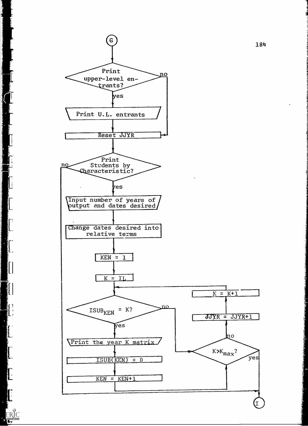
Printupper-level en-

.

no

es

7,1;t U.L. entrants -7

1-41

no

es

\Input number of years77utput and dates desired

Change dates desired intorelative terms

KEN = 1

[ K IL

K+1

I[ MYR = JJYR+1

184

yes

\Print the year K mat-

1

I

KEN KEN+1

ISUB(KEN) = 0

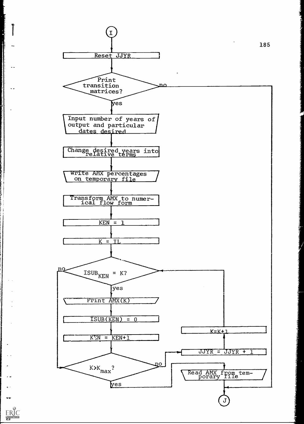
I

Reset JJYR

185

Printtransition

matrices?

Input number of years ofoutput and particular

dat

!Change destired years intoirelaive terms

Write AMX percentages /on temporary file

Transform AMX to numer- 1ical flow form

KEN =

TL

ISUB = K?K N

yes

\ ----Print ATM TO

IsuB(K,N) = 0

K N = KEN+1

ead AMX fl2 m tem-porary r le

es

Store smoothed AMX foryear prior to changedIyear back in o AMY

LDO= -1

Set limits of years usedas observations

186

Zero transition matrixrow sums and elements forappropriate ears

yes

et. ower limit onprojected years

an wr ina ro riate ear limits

input the year tobe chap ed

Store unsinoothed,AMX from year prioto changed year ini

s LDO positive?

Zero aggregate vectors foprojected yrs.,changed yr.

'Zero matrices of total i

students by classificatioand category for projecteand changed ears

Zero the aggregates of thtotal student vectors forprojected and chan ed rs.

input method for next

set of projections

Set (year) limits on ob-servations to be used forcalculation of Reg. Coeff.

Zero matrices of regres-sion coefficients

187

s

no

ILDO =

tet upper limit onrojected

et lower limit onrojected ears

188

npu varia e toh an a

Either AT or AE is tbe changed. Inputrow and no. of ele-ents in it to bechanged; put category no.'s of therhanps into TSUR

\Input the changesinto VALS

KEN =

I = 1 I

Transition matrix isto be changed. Inpuow and no. of ele-ments in it to bechanged; put col-umn no.'s of thenan es into ISUB

Input the changesinto VALS

KEN =

189

Add VALS(KEN) toeither AT or AE,whichever was called

ISUB(K N)

VALS(KEN) =

KEN=KEN+1 j

\Inpuo

t whether an-other change des-

Input whether an-other. change des-ire in same var.

IM7 = 1

e ower im. on prod. yrs.

IStore smoothed AMX for yearprior to the changed year

190

APPENDIX 4.B

nUDSON VALLEY QUESTIONNAIRE

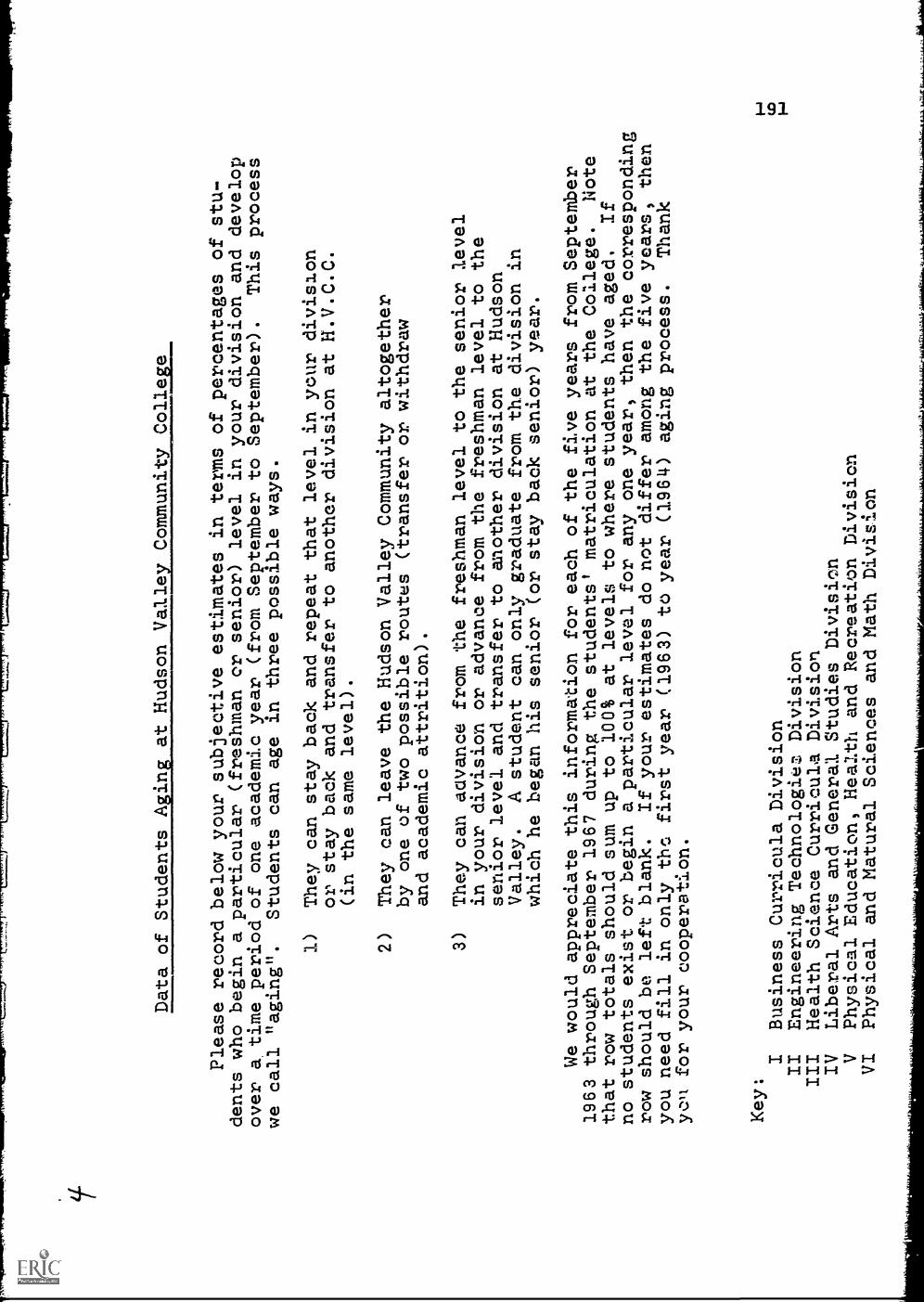
Data of Students Aging at Hudson Valley Community College

Please record below your subjective estimates in terms of percentages of stu-

dents who begin a particular (freshman cr senior) level in your division and develop

over a time period of one academic year (from September to September).

This process

we call "aging".

Students can age in three possible ways.

1)

They can stay back and repeat that level in your division

or stay back and transfer to another division at H.V.C.C.

(in the same level).

2)

They can leave the Hudson Valley Community altogether

by one of two possible routes (transfer or withdraw

and academic attrition).

3)

They can aavance from the freshman level to the senior level

in your division or advance from the freshman level to the

senior level and transfer to another division at Hudson

Valley.

A student can only graduate from the division in

which he began his senior (or stay back senior) year.

We would appreciate this information for each of the five years from September

1963 through September 1967 during the students' matriculation at the College.

Note

that row totals should sum up to 100% at levels to where students have aged.

If

no students exist or begin a particular level for any one year, then the corresponding

row should be left blank.

If your estimates do not differ among the five years, then

you need fill in only thc first year (1963) to year (1964) aging process.

Thank

ycll for your cooperation.

Key:

IBusiness Curricula Division

II

Engineering Technological Division

III

Health Science Curricula Division

IV

Liberal Arts and General Studies Divisicn

VPhysical Education, Health and Recreation Division

VI

Physical and Matural Sciences and Math Division

Fall 1964

Fall 1963

100% of

Students

Age From

Freshman

Level In

Division

I

Students Age To

Freshman Level

Outside World by

,Apnior_Level

III

III

Transfer or

Is

-!.. =

Academic Co

II

III

IV

VVI

Fall 1964

Fall 1963

100% of

Students

Age From

Senior

Level In

Division

I.M.

Students Age To

Senior

Level

IV

VVI

Outside World

17Fa=67Or

Withdrawal

by

ca enact

Attrition

Completion of

De-ree Proeram

.M10

.'

Division I

III

III

OiP

l..d

Fall 1965

...

Fall 1964

100% of

Students

Age From

Freshman

Level In

Division

I

Students Age To

I

Freshman

II

Level

IV

Outside World b

Senior Level

III

VVI

rans er or

Withdrawal

cademic

Attrition

III

III

IV

V

Fall 1965

Fall 1964

100% of

Students

Age From

Senior

Level In

Division

I

..

___.

Students Age To

.....

III

IIIIII

....

Completion of

Senior Level

Outside World by

De ree Pro: ram

III

IV

VVI

Transfer or

Withdrawal

ca emic

Attrition

Division I

1-J

Fall 1966

Fall 19651

100% of

Students

Age From

Freshman

Level In

Division

I

..-----------...................--

Students Age To

b.--

Freshman Level

Outside World by.,

Senior Level

III

III

IV

VVI

Transfer or

Withdrawal

.oademio

Attrition

.......

III

in

Iv

VVI

,

11 S

EN

OM

MIM

I

Fall 1966

Fail 1965

100% of

Students

Age From

Senior

Level in

Division

I

0110W.WW

Students Age To

....

..............

Completion of

Senior Level

Outside World by

Degree Program

."---Trans

II

III

IV

VVI

er or

Withdrawal

ca emIc

Attrition

Division 1

MO

Mm

lMM

P10W

'L

ima.

Fall 1967

Fall 1966

100% of

Students

Age From

Freshman

Level In

Division

I

Students Age To

..0.....

.

I°"'

Freshman Level

,...

4-....................,.

...,.....

....--........

Outside World b

Senior lAevel.

II

III

IV

VVI

rans er or

Withdrawal

.%,..-.....4e

ca emic

Attrition

b.

III

III

IV

VVI

.. Fall 1967

Fall 1966

100% of

Students

Age From

Students Age To

4111

""'I°

1"'"n

Seni

orLevel

Outside World

1=7717 or

Withdrawal

by

...,

Academic

Attrition

MO

M!

Completion of

Degree Program

Division I

Senior

Level In

Division

I

III-II

IIV

....-4.--....-.....

VVI

...--........

dui

2L-101114

ttF-71

r1

9U

c-47

c--1

'

Fall 1968

774

F1=

41=.1

Fall 1967

100% of

Students

Age From

Freshman

Level In

Division

I

Students Age To

.-

VI.M

INN

O

Freshman Level

Outside World b

Senior Level

III

III

IV

VVI

rans er or

'Withdrawal

'cademic

Attrition

III

III

IV

VVI

Fall 1968

Fall 1967

100% of

Students

Age From

Senior

Level In

Division

I

Students Age To

_

Completion of

Senior Level

Outside World by

Degree Program

III

III

IV

VVI

Transfer or

Withdrawal

cademio

Attrition

Division I

.....

to 0)

197

Please estimate the percent of male students in each level

in your division for the beginning of the following academic

years.

Fail Freshman Senior

1963

1964

1965

1966

1967

Please estimate the percent of students in the senior level

in your division which have transferred to H.V.C.C. from

another school for the beginning of each of the following

academic years.Please estimate the percent of these transfers which are male.

Percent of Seniors Percent of transfers

Fall which are Transfers which are male

1963

1964

1965

1966

1967

198

FOOTNOTES

1. Rensselaer Research Corporation, The Development ofa Computer Model for Projecting Statewide CollegeEnrollments: A Preliminary Study (Prepared for theOffice of Planning in Higher Education, StateEducation Department, University of the State ofNew York, January 7, 1968.

2. Zabrowski, E. K., Zinter, J. R., and Okada, T.,Student-Teacher Population Growth Model, U. S.Department of Health, Education and Welfare, OE-10055,National Center for Educational Statistics, 1958.

3. Thonstad, T., "A Mathematical Model of the NorwieganEducational System" Mathematical Models in EducationalPlanning, OECD, Paris, 1967, pp. 125-158.

4. Gani, J., "Formulae for Projecting Enrollments andDegrees Awarded in Universities," Journal of theRoyal statistical Society, Vol. 120, Part 3, 1963,pp. 400-409. (See also Chapter II ofBartholomew, D. J., Stochastic Models for SocialProcesses, John Wiley and Sons, 1967.

5. Koenig, H. E., Keeney, M. G., and Zemach, R.,A Systems Model for Management, Planning, andResource Allocation in Institutions of HigherEducation, DivisiRT7Of Engineering Research, MichiganState University, September 30, 1968.

6. See the Report of the Select Committee on the Futureof Private and Independent Higher Education in New'fork State (The Bundy Report). It's overridingpurpose was to determine "how the state can helppreserve the strength and vitality of our private andindependent institutions of higher education, and yetat the same time keep them free."

Serving the developmert needs of government and industry

Rensselaer Research Corporation1125 Peoples Avenue, Troy, New York 12181