do urban land regulations influence slum formation?...

1

Do Urban Land Regulations Influence Slum Formation? Evidence from Brazilian Cities1

Somik V. Lall†, Hyoung Gun Wang† and Daniel da Mata*

† The World Bank, Washington DC, USA

* Instituto de Pesquisa Econômica Aplicada (IPEA), Brasilia, Brazil

Draft 2: July 24, 2006

Abstract In this paper, we examine the effects of land use zoning and density regulations on formal housing supply and slum formation across Brazilian cities between 1980 and 2000. In particular we look at the performance of cities that have lowered land subdivision (minimum lot size) regulation from the federally mandated 125 m2. We develop a model of formal housing supply and slum formation where population growth is endogenous and household migration decisions are influenced by inter city variations in land regulations. We find that the elasticity of formal housing supply in Brazil is very low, and comparable to those found in Malaysia and South Korea, which have highly regulated housing markets. Our analysis of land regulations shows that (a) general purpose zoning and land use planning improves performance of the housing market and stimulates formal sector housing response, thereby reducing slum formation; (b) lowering minimum lot size regulations increases housing supply but is also accompanied by higher population growth. We find that population growth is faster than the formal housing supply response, leading to an increase in slum formation. This suggests that policies that aim to reduce barriers for access to land need to be accompanied by instruments that relax pre-existing distortions in the land market. In the absence of these measures, pro poor land regulations may in fact exacerbate the slum formation problem.

1 This research has been funded by a World Bank Knowledge for Change (KCP) program grant “Dynamics of Slum Formation and Strategies to Improve Lives of Slum Dwellers.” The findings reported in this paper are those of the authors alone, and should not be attributed to IPEA or the World Bank, its executive directors, or the countries they represent. We thank Mila Freire for helpful comments. Author for correspondence: Somik V. Lall; Senior Economist, Development Research Group, The World Bank. Email: [email protected].

2

1. BACKGROUND AND MOTIVATION

There is considerable evidence to show that the number of urban residents living in slums

is growing rapidly globally. Current estimates suggest that there are more than 1 billion

slum dwellers worldwide, who account for about 32 percent of the global urban

population (United Nations 2003). With continuing rapid growth of urban areas,

improving the lives of slum dwellers is a high priority for national and city governments

and the international development community. The Millennium Development Goals, for

instance, advocate significant improvements in the lives of at least 100 million slum

dwellers by 2020 (United Nations, 2005). However, at this time there is very little

empirical evidence on the determinants of slum formation and identifying local and

national policy environments that influence the capacity of cities to manage the growth of

slums.

In this paper, our main objective is to examine if specific local innovations and

policies are associated with managing the rate of slum formation. In particular, we focus

our attention on urban land use and zoning policies, which have been found to influence

(formal) land prices (Glaeser et al. 2002 (USA), World Bank 2005 (India), 2004

(Bangladesh), local revenue collection (Smolka and De Cesare, 2006), and informal

housing development (XXX). We explicitly examine how household migration and

residential location decisions interact with city level policies that govern the functioning

of the land and housing markets. In terms of local policies, we examine the influence of

land use and zoning regulations in improving the city’s capacity to absorb new residents.

We start with the prior that slums (or informal sector housing) are a response to the

failure of the formal housing market to meet market demand. The supply elasticity of the

3

formal housing market may be influenced by land management regulations, which make

new formal developments unaffordable relative to incomes for the poor.

We use data from Brazilian cities to empirically examine how two particular land

management instruments – land use zoning and minimum lot size regulations influence

migration and slum formation. Let us consider how each of these instruments operates.

Zoning regulations typically allocate land among different uses to best reflect community

preferences and prevent incompatible uses from being located near one another. In

general, zoning ensures that land is managed efficiently and stimulates the development

of a functioning formal land and housing market. This should increase the elasticity of

formal land and housing supply in response to demand and manage the rate of informal

housing/ slum formation.

Some zoning regulations such as density controls are often put in place to help

public authorities in planning for the provision of public services such as sewage, roads,

public schools, health services and transportation. These density controls include

minimum lot size regulations (or regulations on land sub division) and setting floor area

ratios (FARs), which specify the limit to vertical development on a plot of land. In 1979

the Federal government in Brazil established the basic legislation at the national level

(Federal Law 6766) for developing, approving and registering urban land subdivisions

(World Bank 2006). Among these parameters are a minimum lot size of 125 m², with a

minimum frontage of 5 m, and a compulsory donation of 35% of development area for

public uses and open spaces. However, the Federal Law (article 4) allows states and

municipalities to waive federal subdivision regulations and lower the minimum lot size

4

for land to be set aside for developing low income housing. These areas are called Special

Zones of Social Interest (ZEIS; Zonas Especiais de Habitacao de Interesse Social).

Several cities such as Recife, Belo Horizonte, Porto Alegre and Belém have

classified parts of their jurisdiction as ZEIS to regularize informal settlements and

produce affordable houses for the poor. These ZEIS have flexible zoning regulations such

as reduced minimum lot sizes (90 m² in Belem, 50 m² in Fortaleza, and 40 m² in Belo

Horizonte) and variable frontage (World Bank 2006).

In the empirical analysis, we examine how the presence of general zoning laws

and flexibility in defining minimum lot sizes influence formal housing supply and slum

formation across Brazilian cities between 1980 and 2000. While general purpose land use

allocations should improve the functioning of the formal land and housing markets, large

lot regulations would raise the effective house price to income ratio in the short term, and

make formal housing unaffordable for many residents – particularly the poor. As a

consequence, there is a substitution effect and households choose to live in informal

settlements- either by purchasing informally subdivided land or houses built on such

developments. The long term implication of these regulations is however ambiguous.

These regulations may serve as newcomer taxes for potential migrants, and may in fact

reduce migration into the city. If the barriers to entry are sufficiently strong, the demand

on the formal supply system will drop and slum formation may possibly slow down.

However, the extent to which drop in migration is accompanied with an increase in

formal housing supply remains an empirical question.

The rest of the paper is organized as follows. In Section 2, we describe patterns of

slum formation in Brazil between 1980 and 2000. Next, we begin the empirical

5

investigation by estimating the elasticity of formal housing supply to meet additional

demand, and the implications of inelastic supply response in terms of slum formation.

This is reported in Section 3. In Section 4, we outline a model and estimation framework

to examine the determinants of slum formation. In Section 5, we discuss results from the

econometric analysis and focus our attention on the effects of zoning regulations. Section

6 concludes.

2. SLUM FORMATION IN BRAZIL

Access to urban land and housing in Brazil has mostly relied on (1) the division of

central and peripheral land (loteamentos) and (2) the invasion of public and private urban

land (favelas). As a result, in main cities modern central areas are surrounded by irregular

and illegal settlements which lack in drainage and sewerage systems, health and

education facilities, and green spaces. Public transport is insufficient and expensive, and

the quality of life in slums is very low.

What constitutes a slum? There are three forms of slums in Brazil: Favelas,

cortiços, and irregular/clandestine loteamentos. Favelas are the most common form of

slums in Brazilian cities.2 They are illegal settlements arising mainly from the invasion of

public and private urban land. These invaded areas are generally located close to city

centers, but mostly unsuitable for human occupation due to geographical and ecological

factors. They lack in almost every element of urban infrastructure. Cortiços are high

density collective housing in city centers. They are old and subdivided into small rooms

with many fire hazards, few bathrooms, no formal rental relationships, no proof of

2 The name comes from a mountain (Morro de Favela) in the center of Rio de Janeiro, occupied by squatters in 1906.

6

payments, and often run by intermediaries connected to the police and criminals (Saule

1999). Loteamentos are usually developed in peripheral areas irregularly, if not also

illegally. These land divisions typically do not comply with building quality or safety

regulations and not registered in the public registry office. Loteamentos developed in

areas of contested ownership are called “clandestine.” They differ from favelas, since the

occupiers have bought their plots from whoever presented themselves as landowners, and

in most cases paid all due taxes.

Slum formation in Brazil: The slum definition and data that we use in this analysis

come from the Brazilian Geography and Statistics Institute (IBGE). As per IBGE’s

definition, a slum is a “subnormal agglomeration”, which satisfies the following three

conditions: (i) a nucleus (group) made up of over 50 housing units, (ii) land occupation is

illegal, and (iii) meets at least one of the following criteria of (a) urbanization in a

disordered pattern (for example, narrow and winding roads) and (b) lack of essential

public services and utilities.3 The IBGE definition has limitations such that it would

under count residents in Cortiços and some Loteamentos. This is evident in comparisons

of IBGE slum data with other survey data sources. For example, a 1993 survey in Sao

Paulo done by the Economic Research Institute Foundation of the University of Sao

Paulo reported 1.9 million slum dwellers (19.8% of the population), but the IBGE census

in 1996 affirmed only 748,000 slum dwellers in the city, the equivalent of 7.6% of the

population (Fix et al., 2003). However, the IBGE data are the most comprehensive and

systematically compiled source that can be used for examining slum formation across the

Brazilian urban system.

3 The housing unit must have at least two public services (for example, electricity and piped water, or piped water and sewage) in order not to be considered as a slum.

7

Our analysis is based on IBGE slum data from the Population Censuses of 1980,

1991, and 2000. Our sample consists of 123 agglomerations, which includes 447 MCAs

(Minimum Comparable Areas). We link the dataset developed in Da Mata et. al (2005) to

slum formation rates for this analysis. Appendix A provides a detailed description of data

sources and variable definitions used in this analysis.

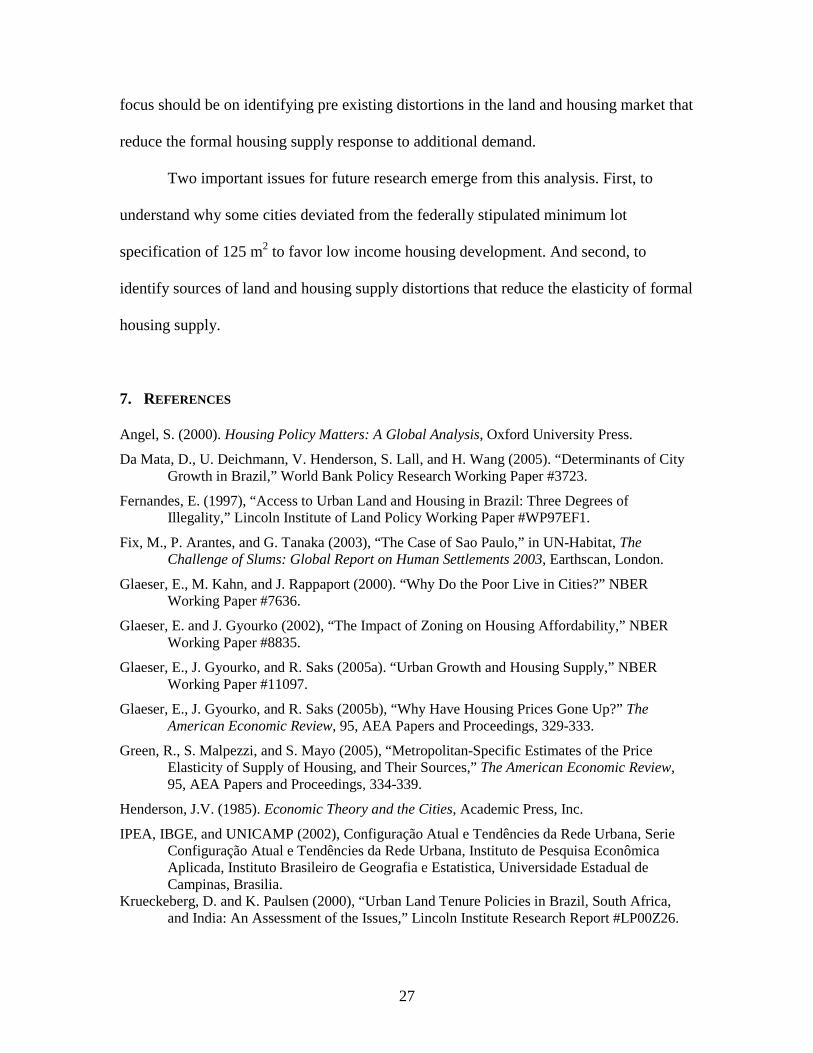
In Table 1, we present summary statistics of city population, housing stock, slum

dwellers and slum units. The growth of slum dwellers and slum units in cities has been

much higher than those of total city population and housing stock. The annual growth

rates of slum dwellers in cities in the 1980s and 1990s were 5.5% and 3.9%, respectively

which are much higher than city population growth (2.4% and 2.0%) as a whole. As a

result, the share of slum dwellers relative to city population increased from 3.6% in 1980

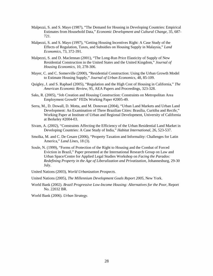
to 6.0% in 2000. Across cities, we find in Table 2 that the largest cities have the highest

rates of slum formation in 2000. The four largest cities (with populations more than 4.2

million) collectively have 3.6 million slum dwellers, accounting for 9.1% of the total

population. At the lower end of the urban hierarchy, there are 57 small cities with less

than 202,000 people, where slum dwellers only account for 1.2 % of the total population.

At the same time the share of formal houses relative to the total housing stock decreases

as city size increases. (see Table 2)

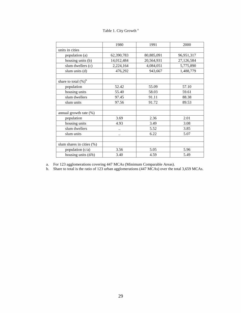
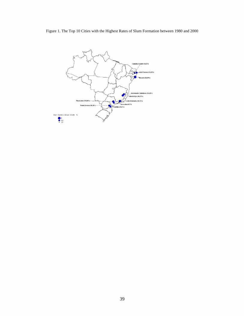
Figure 1 displays the top ten cities in terms of slum formation rates between 1980

and 2000. Most of these cities are located along the southern coastline, suggesting that

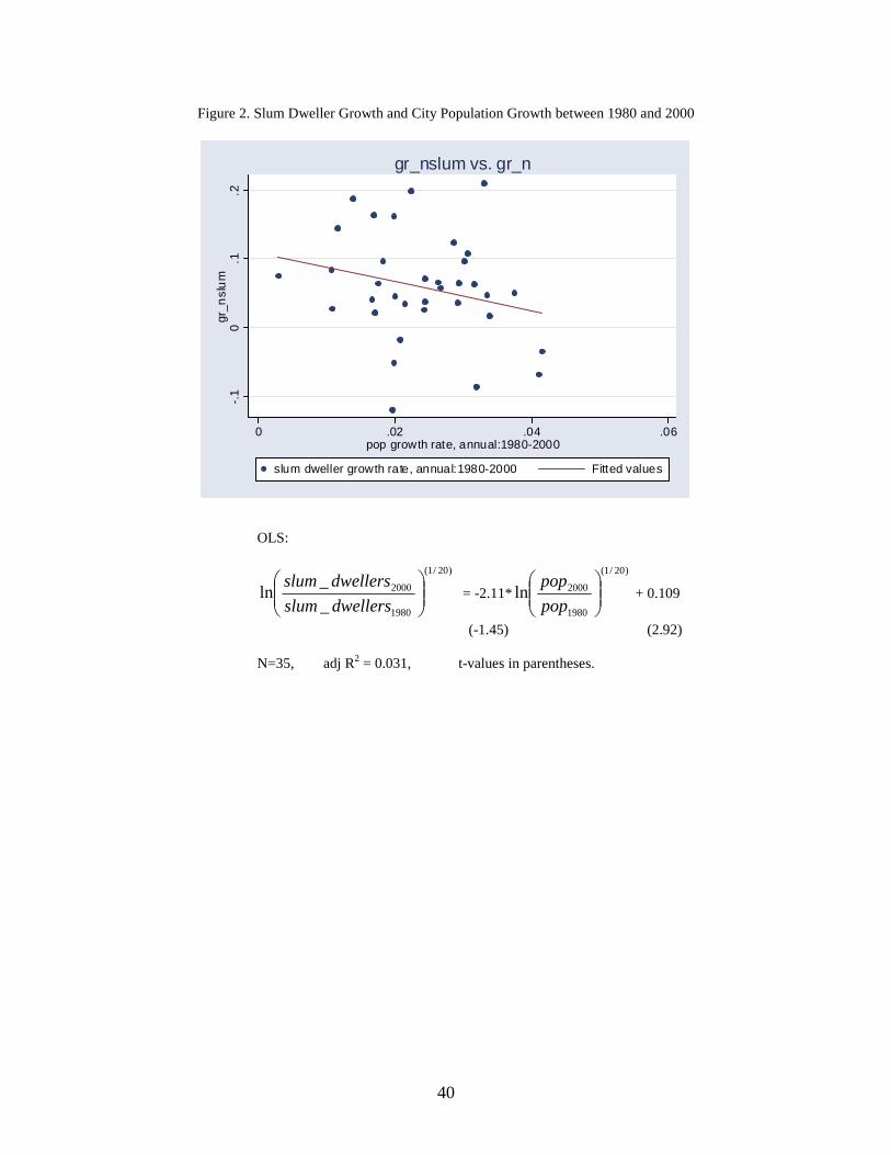
local and regional characteristics may influence slum formation. Interestingly, Figure 2

and the corresponding OLS regression show no statistically significant relationship

between slum growth and city population growth. This would suggest that slum

8

formation is a complicated process influenced by various city characteristics, rather than

simply proportional to city size growth itself.

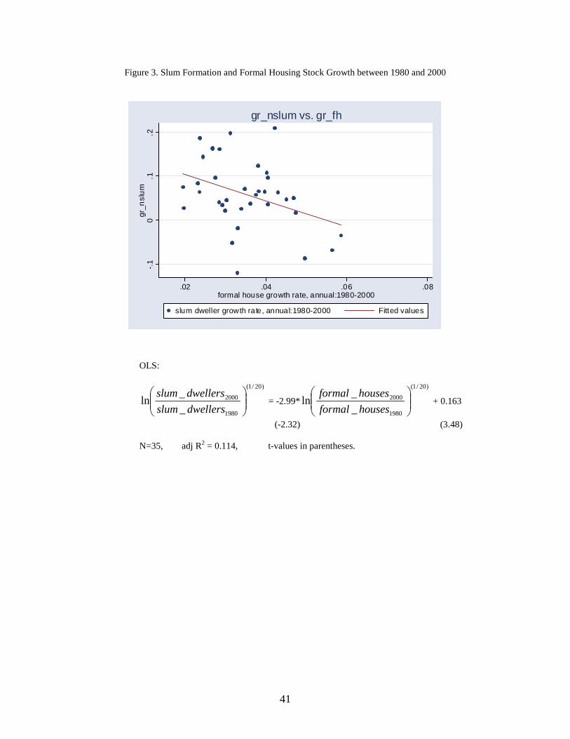
Figure 3 and corresponding OLS result show a statistically significant and

negative relationship between the slum growth and the growth of formal housing stock

between 1980 and 2000.4 For example, the two cities in the bottom right of Figure 3 are

Cuiabá and Campo Grande. These two cities successfully increased formal housing stock

at the annual growth rates of 5.9% and 5.6% respectively between 1980 and 2000, and

were able to manage slum formation (slum growth rates are -3.5% and -6.9% annually).

In the following two sections, we identify factors that influence formal housing

supply and slum formation. Section 3 considers short term effects where we focus on the

functioning of the formal housing market and the price elasticity of housing supply. We

assume the size of formal housing market to be fixed, i.e., the number of households who

buy formal houses is exogenously given. In Section 4, we extend this model by allowing

households to migrate across cities and choose whether to live in formal or informal

developments. Therefore, growth of the formal housing market and city population are

endogenously determined. Slums are created when mobile households decide to build

houses “informally” in the city.

3. FORMAL HOUSING SUPPLY

Recent empirical research suggests that the elasticity of housing supply varies

significantly across cities within a country (Green, Malpezzi, and Mayo 2005) and across

countries (Malpezzi and Mayo 1997; and Malpezzi and Maclennan 2001), and that these

4 Formal housing stock is defined by the difference between the number of total housing units and the number of slum units.

9

differences are mainly driven by restrictive zoning and other land use regulations (Saks,

2005; Glaeser, Gyourko, and Saks, 2005a,b; Green, Malpezzi, and Mayo, 2005; Quigley

and Raphael, 2005). Much of the existing empirical evidence is based on data from

developed countries, particularly the United States where market clearing is implicitly

assumed: i.e. housing prices and the housing stock adjust to external shocks, and the

housing market is in equilibrium. However, this market clearing assumption is unlikely to

hold in many developing countries where the capacity of the formal housing market is so

limited that the urban poor and even middle income households resort to informal

housing solutions.

In our analysis, we distinguish between formal and informal housing sectors.

When city regulations make it difficult for residents to enter the formal housing market,

housing demand will be met via informal solutions. In this regard, the price elasticity of

housing supply measures the capacity of the formal housing sector to absorb urban

migrants into the system. Inelastic housing supply limits the housing stock adjustment in

response to migration and urban expansion, and therefore stimulates slum formation. We

develop a slum formation model which accounts for this housing market disequilibrium.

This model provides the framework for our empirical work. We estimate a reduced form

equation for the formal housing market.

10

Aggregate Formal Housing Market

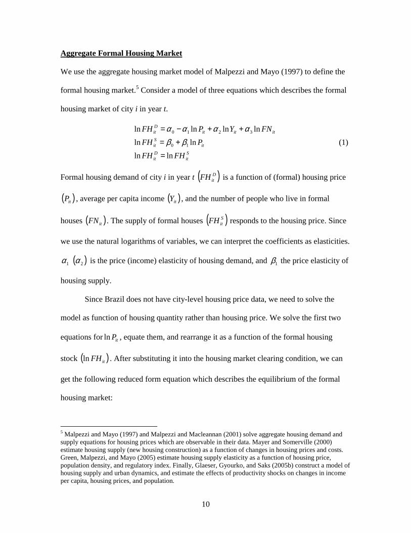
We use the aggregate housing market model of Malpezzi and Mayo (1997) to define the

formal housing market.5 Consider a model of three equations which describes the formal

housing market of city i in year t.

Sit

Dit

itSit

itititDit

FHFH

PFH

FNYPFH

lnln

lnln

lnlnlnln

10

3210

=

+=

++−=

ββαααα

(1)

Formal housing demand of city i in year t ( )DitFH is a function of (formal) housing price

( )itP , average per capita income ( )itY , and the number of people who live in formal

houses ( )itFN . The supply of formal houses ( )SitFH responds to the housing price. Since

we use the natural logarithms of variables, we can interpret the coefficients as elasticities.

1α ( )2α is the price (income) elasticity of housing demand, and 1β the price elasticity of

housing supply.

Since Brazil does not have city-level housing price data, we need to solve the

model as function of housing quantity rather than housing price. We solve the first two

equations for itPln , equate them, and rearrange it as a function of the formal housing

stock ( )itFHln . After substituting it into the housing market clearing condition, we can

get the following reduced form equation which describes the equilibrium of the formal

housing market:

5 Malpezzi and Mayo (1997) and Malpezzi and Macleannan (2001) solve aggregate housing demand and supply equations for housing prices which are observable in their data. Mayer and Somerville (2000) estimate housing supply (new housing construction) as a function of changes in housing prices and costs. Green, Malpezzi, and Mayo (2005) estimate housing supply elasticity as a function of housing price, population density, and regulatory index. Finally, Glaeser, Gyourko, and Saks (2005b) construct a model of housing supply and urban dynamics, and estimate the effects of productivity shocks on changes in income per capita, housing prices, and population.

11

ititit FNYFH lnlnln11

13

11

12

11

0110

βαβα

βαβα

βαβαβα

++

++

++= (2)

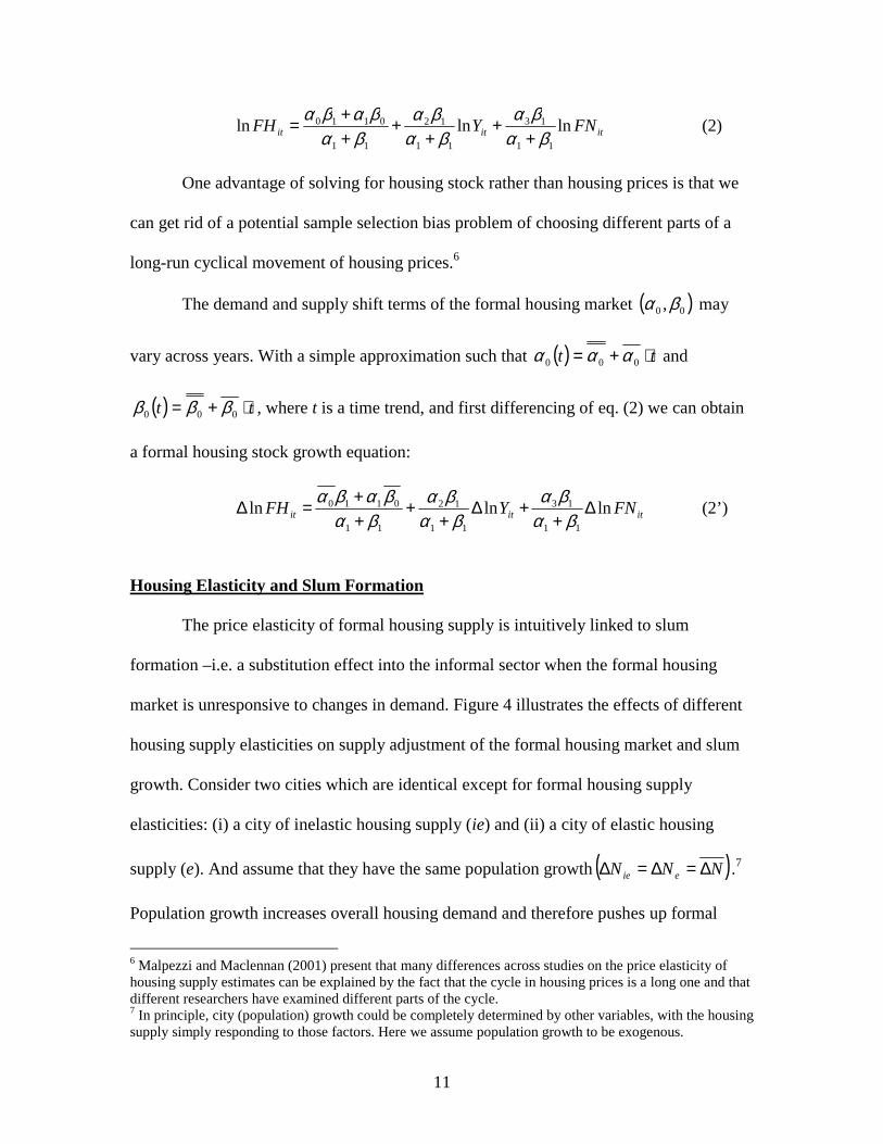
One advantage of solving for housing stock rather than housing prices is that we

can get rid of a potential sample selection bias problem of choosing different parts of a

long-run cyclical movement of housing prices.6

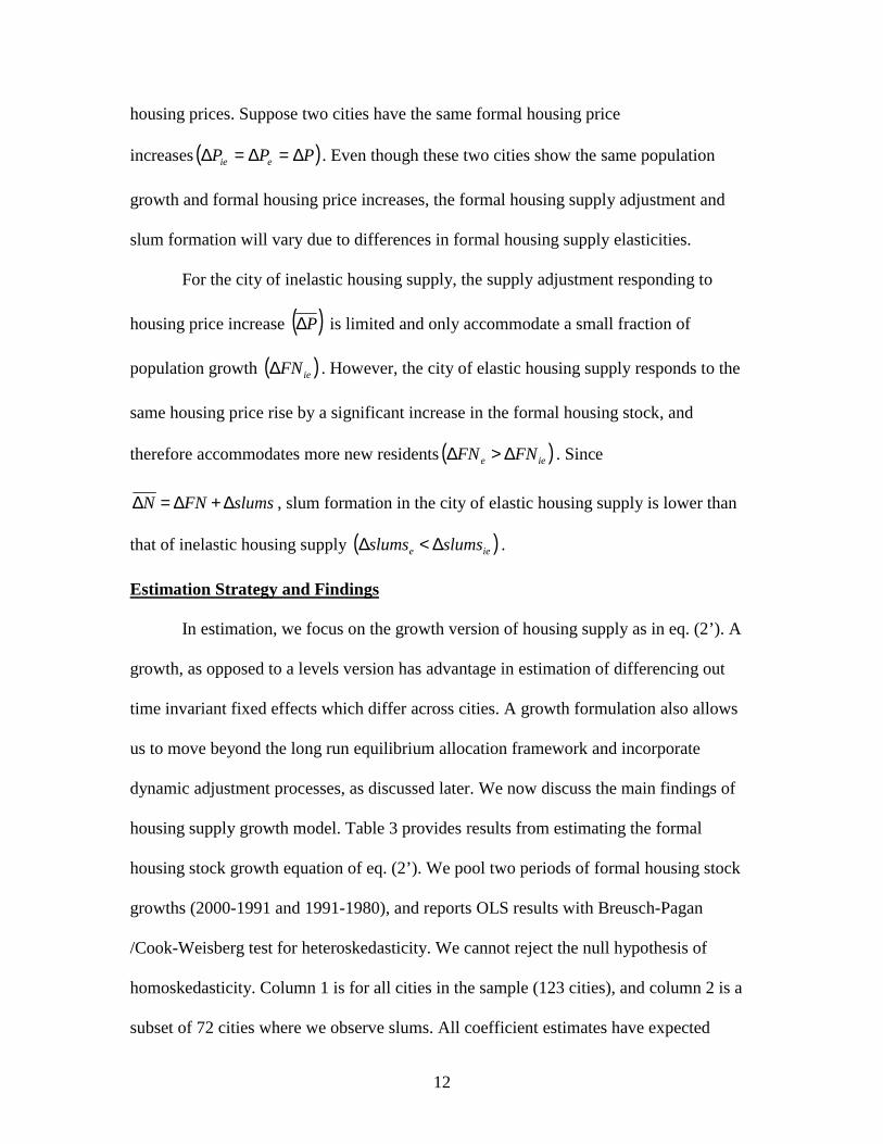
The demand and supply shift terms of the formal housing market ( )00 ,βα may

vary across years. With a simple approximation such that ( ) tt ⋅+= 000 ααα and

( ) tt ⋅+= 000 βββ , where t is a time trend, and first differencing of eq. (2) we can obtain

a formal housing stock growth equation:

ititit FNYFH lnlnln11

13

11

12

11

0110 ∆+

+∆+

+++=∆

βαβα

βαβα

βαβαβα

(2’)

Housing Elasticity and Slum Formation

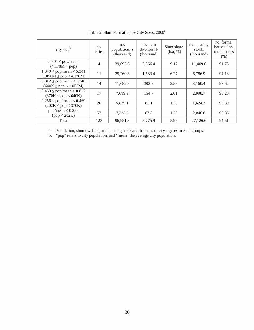
The price elasticity of formal housing supply is intuitively linked to slum

formation –i.e. a substitution effect into the informal sector when the formal housing

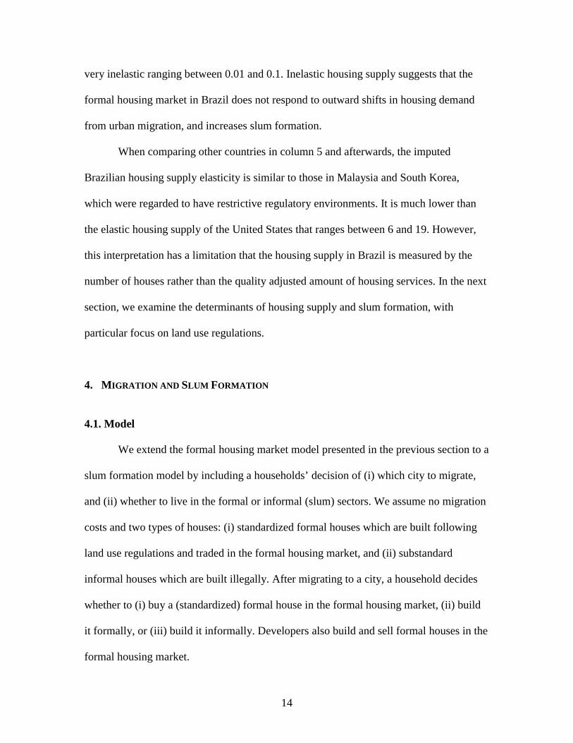
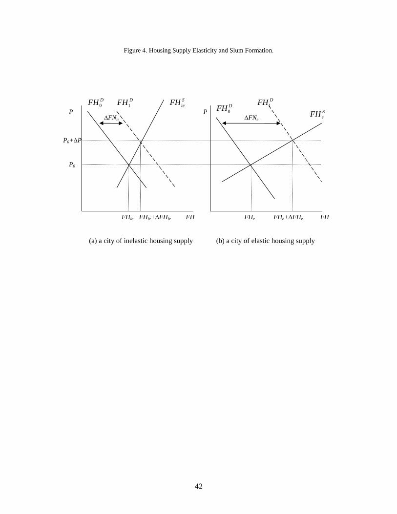
market is unresponsive to changes in demand. Figure 4 illustrates the effects of different

housing supply elasticities on supply adjustment of the formal housing market and slum

growth. Consider two cities which are identical except for formal housing supply

elasticities: (i) a city of inelastic housing supply (ie) and (ii) a city of elastic housing

supply (e). And assume that they have the same population growth ( )NNN eie ∆=∆=∆ .7

Population growth increases overall housing demand and therefore pushes up formal

6 Malpezzi and Maclennan (2001) present that many differences across studies on the price elasticity of housing supply estimates can be explained by the fact that the cycle in housing prices is a long one and that different researchers have examined different parts of the cycle. 7 In principle, city (population) growth could be completely determined by other variables, with the housing supply simply responding to those factors. Here we assume population growth to be exogenous.

12

housing prices. Suppose two cities have the same formal housing price

increases ( )PPP eie ∆=∆=∆ . Even though these two cities show the same population

growth and formal housing price increases, the formal housing supply adjustment and

slum formation will vary due to differences in formal housing supply elasticities.

For the city of inelastic housing supply, the supply adjustment responding to

housing price increase ( )P∆ is limited and only accommodate a small fraction of

population growth ( )ieFN∆ . However, the city of elastic housing supply responds to the

same housing price rise by a significant increase in the formal housing stock, and

therefore accommodates more new residents ( )iee FNFN ∆>∆ . Since

slumsFNN ∆+∆=∆ , slum formation in the city of elastic housing supply is lower than

that of inelastic housing supply ( )iee slumsslums ∆<∆ .

Estimation Strategy and Findings

In estimation, we focus on the growth version of housing supply as in eq. (2’). A

growth, as opposed to a levels version has advantage in estimation of differencing out

time invariant fixed effects which differ across cities. A growth formulation also allows

us to move beyond the long run equilibrium allocation framework and incorporate

dynamic adjustment processes, as discussed later. We now discuss the main findings of

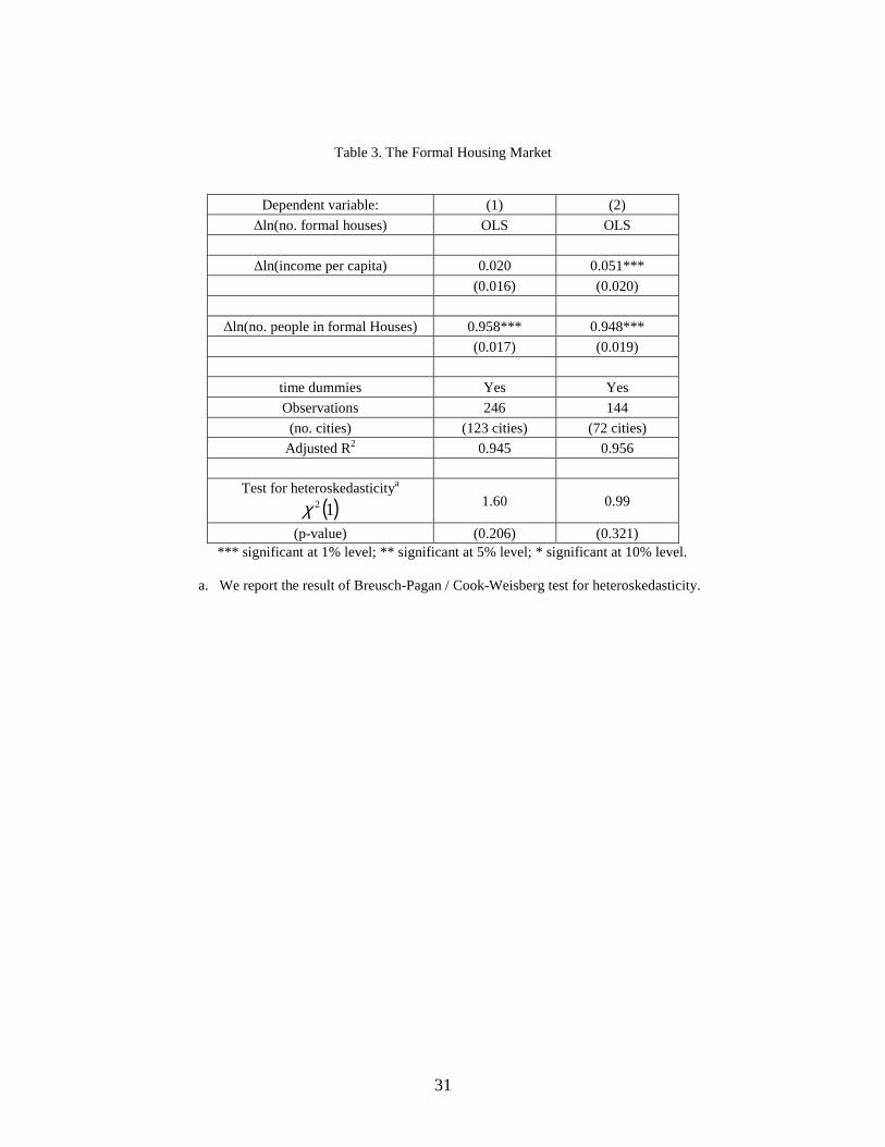
housing supply growth model. Table 3 provides results from estimating the formal

housing stock growth equation of eq. (2’). We pool two periods of formal housing stock

growths (2000-1991 and 1991-1980), and reports OLS results with Breusch-Pagan

/Cook-Weisberg test for heteroskedasticity. We cannot reject the null hypothesis of

homoskedasticity. Column 1 is for all cities in the sample (123 cities), and column 2 is a

subset of 72 cities where we observe slums. All coefficient estimates have expected

13

signs, and are statistically significant except for per capita income in column 1. Both

growth in per capita income and formal house residents raises the growth rate of the

formal housing stock.

As illustrated in Figure 4, if a city’s formal housing supply is elastic, an outward

shift in housing demand results in a large increase in housing stock and a relatively

modest housing price increase. However, if housing supply is inelastic, we expect less

supply adjustment and significant housing price increases. In this regard, the price

elasticity of housing supply has an important policy implication. However, we cannot

directly measure the housing supply elasticity due to a standard identification problem.8

Malpezzi and Mayo (1997) and Malpezzi and Macleannan (2001) solve this problem by

assuming the housing demand elasticities to be in a certain range.

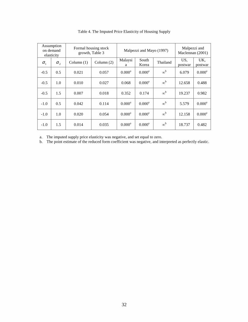
Malpezzi and Mayo (1997) suggest that reasonable bounds for the price elasticity

of housing demand would be between -0.5 and -1.0, and the long-run income elasticity

between 1.0 and 1.5. Malpezzi and Macleannan (2001) also propose similar bounds for

the United States and the United Kingdom: between -0.5 and -1.0 for the price elasticity

of demand, and between 0.5 and 1.0 for the long-run income elasticity of demand. Table

4 calculates the imputed price elasticity of housing supply ( )1̂β based on coefficient

estimates in Table 3. The calculation is from a range of assumptions about housing

demand elasticities ( )21 ,aα mentioned above. We assume the price elasticity of housing

demand ( )1α to be between -0.5 and -1.0, and the income elasticity of housing demand

( )2α between 0.5 and 1.5. The imputed price elasticity of housing supply turns out to be

8 In eq. (2’), we have 4 parameters ( )1321 ,,, βαα a which cannot be identified from 2 coefficient

estimates

+

=+

=11

132

11

121

ˆ,ˆβα

βαβα

βαbb .

14

very inelastic ranging between 0.01 and 0.1. Inelastic housing supply suggests that the

formal housing market in Brazil does not respond to outward shifts in housing demand

from urban migration, and increases slum formation.

When comparing other countries in column 5 and afterwards, the imputed

Brazilian housing supply elasticity is similar to those in Malaysia and South Korea,

which were regarded to have restrictive regulatory environments. It is much lower than

the elastic housing supply of the United States that ranges between 6 and 19. However,

this interpretation has a limitation that the housing supply in Brazil is measured by the

number of houses rather than the quality adjusted amount of housing services. In the next

section, we examine the determinants of housing supply and slum formation, with

particular focus on land use regulations.

4. MIGRATION AND SLUM FORMATION

4.1. Model

We extend the formal housing market model presented in the previous section to a

slum formation model by including a households’ decision of (i) which city to migrate,

and (ii) whether to live in the formal or informal (slum) sectors. We assume no migration

costs and two types of houses: (i) standardized formal houses which are built following

land use regulations and traded in the formal housing market, and (ii) substandard

informal houses which are built illegally. After migrating to a city, a household decides

whether to (i) buy a (standardized) formal house in the formal housing market, (ii) build

it formally, or (iii) build it informally. Developers also build and sell formal houses in the

formal housing market.

15

Migration decision

Suppose that people can migrate freely across cities. Then city communities may exercise

political control over land use within their jurisdiction in order to maximize the welfare

of current city residents. Land use regulations can inhibit migration of the urban poor and

service as a newcomer tax or an exclusionary mechanism. Given this entry barrier, poor

urban migrants are more likely to migrate to cities with less stringent land use

regulations. At the same time, migration decision also depends on real disposable

incomes after paying for houses, or housing price relative to incomes )/( YP . Then

migration, or city population growth, can be formulated as

( )1121101 /lnlnlnlnln −−−− −−=−= ttttt YPdRddNNNd (3)

where R is a measure of stringent land use regulations, and 0, 21 >dd .

A household’s decision to live in the informal sector

We assume that households can measure their hedonic preferences for each housing

types, and that household’s willingness to pay (WTP) for a formal house is greater than

an informal house, such that 0>− IFHFH WTPWTP . However, as various (stringent) land

use regulations (R) increase construction costs, the total construction cost (TC) of a

formal house is greater than that of an informal house: 0)( >− IFHFH TCRTC , where

0)( >

∂⋅∂

R

TC FH

.9 A household builds an informal house, if the construction cost

9 Informal house construction costs are assumed to be fixed, as informal house construction does not comply with cost-increasing regulations.

16

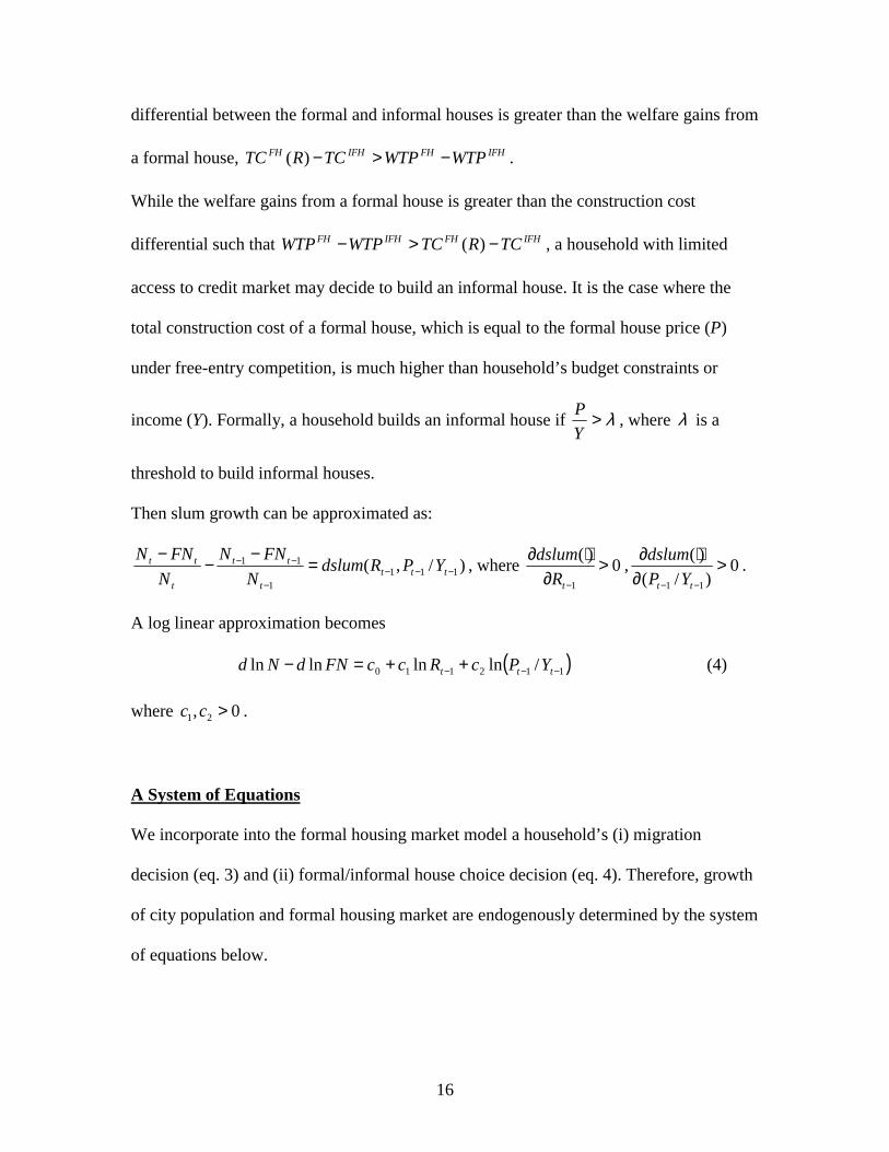
differential between the formal and informal houses is greater than the welfare gains from

a formal house, IFHFHIFHFH WTPWTPTCRTC −>−)( .

While the welfare gains from a formal house is greater than the construction cost

differential such that IFHFHIFHFH TCRTCWTPWTP −>− )( , a household with limited

access to credit market may decide to build an informal house. It is the case where the

total construction cost of a formal house, which is equal to the formal house price (P)

under free-entry competition, is much higher than household’s budget constraints or

income (Y). Formally, a household builds an informal house if λ>Y

P, where λ is a

threshold to build informal houses.

Then slum growth can be approximated as:

)/,( 1111

11−−−

−

−− =−−−ttt

t

tt

t

tt YPRdslumN

FNN

N

FNN, where 0

)(

1

>∂

⋅∂

−tR

dslum, 0

)/(

)(

11

>∂

⋅∂

−− tt YP

dslum.

A log linear approximation becomes

( )112110 /lnlnlnln −−− ++=− ttt YPcRccFNdNd (4)

where 0, 21 >cc .

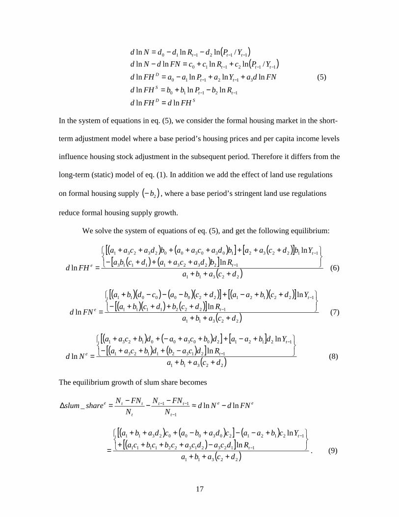
A System of Equations

We incorporate into the formal housing market model a household’s (i) migration

decision (eq. 3) and (ii) formal/informal house choice decision (eq. 4). Therefore, growth

of city population and formal housing market are endogenously determined by the system

of equations below.

17

( )( )

SD

ttS

ttD

ttt

ttt

FHdFHd

RbPbbFHd

FNdaYaPaaFHd

YPcRccFNdNd

YPdRddNd

lnln

lnlnln

lnlnlnln

/lnlnlnln

/lnlnln

12110

312110

112110

112110

=

−+=

++−=

++=−−−=

−−

−−

−−−

−−−

(5)

In the system of equations in eq. (5), we consider the formal housing market in the short-

term adjustment model where a base period’s housing prices and per capita income levels

influence housing stock adjustment in the subsequent period. Therefore it differs from the

long-term (static) model of eq. (1). In addition we add the effect of land use regulations

on formal housing supply ( )2b− , where a base period’s stringent land use regulations

reduce formal housing supply growth.

We solve the system of equations of eq. (5), and get the following equilibrium:

( ) ( )[ ] ( )[ ]( ) ( )[ ]

( )22311

12232311113

112232103030023231

ln

ln

lndcaba

Rbdacaadcba

Ybdcaabdacaabdacaa

FHd t

t

e

+++

++++−++++++++

= −

−

(6)

( )( ) ( )( )[ ] ( )( )[ ]( )( ) ( )[ ]

( )22311

12221111

12212122000011

ln

ln

lndcaba

Rdcbdcba

Ydcbaadcbacdba

FNd t

t

e

+++

++++−++−++−−−+

= −

−

(7)

( ) ( )[ ] [ ]( ) ( )[ ]

( )22311

1213211231

121212003001231

ln

ln

lndcaba

Rdcabdbcaa

Ydbaadbcaadbcaa

Nd t

t

e

+++

−+++−+−+++−+++

= −

−

(8)

The equilibrium growth of slum share becomes

ee

t

tt

t

tte FNdNdN

FNN

N

FNNshareslum lnln_

1

11 −≈−−−=∆−

−−

( ) ( )[ ] ( )( )[ ]

( )22311

1123213221111

121212030002311

ln

ln

dcaba

Rdcadcacbcbca

Ycbaacdabacdaba

t

t

+++

−+++++−−+−+++

= −

−

. (9)

18

Comparative Statics

Land regulation

The effect of land use regulations on slum growth is “ambiguous”, such that

( )( ) 0

ln

_

22311

123213221111

1<>

− +++−+++=

∂∆∂

dcaba

dcadcacbcbca

R

shareslum

t

e

(10)

If a city has strict land use regulations, the current urban poor in the city are likely to

resort to informal housing solutions. However, strict regulations may provide migrant

unfriendly signals to potential newcomers and will inhibit migration, particularly to the

poor. This will reduce new slum formation. Therefore the net effect of whether land use

regulations increase or decrease slum formation depends on the relative sizes of these two

opposing effects.

Income Effect

The income effect on slum growth is also “ambiguous”, such that

( )( ) 0

ln

_

22311

2121

1<>

− ++++−−=

∂∆∂

dcaba

cbaa

Y

shareslum

t

e

(11)

An increase in household income has a direct positive effect on formal house demand,

and therefore decreases slum formation (income effect). However, an increase in formal

house price (due to demand shift-up) will force households to build informal houses

(substitution effect). The net effect depends on the extent to which the formal house price

increases relative to income growth. It can be shown that the rise of formal house prices

is higher than income growth if 0121 <+− baa .10 In this case, economic growth ends up

increasing slum formation. Finally, if the households’ budget constraints does not affect

10 It can be shown from eq. (5) that 2311

232

lnln

caba

caa

Y

P

+++=

∂∂

. Therefore , 1lnln >

∂∂

Y

P if 012 >+− baa .

19

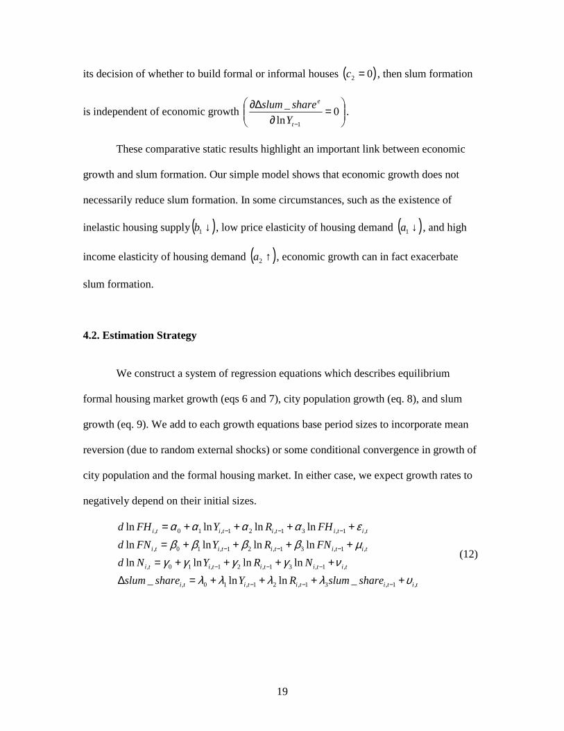
its decision of whether to build formal or informal houses ( )02 =c , then slum formation

is independent of economic growth

=

∂∆∂

−

0ln

_

1t

e

Y

shareslum.

These comparative static results highlight an important link between economic

growth and slum formation. Our simple model shows that economic growth does not

necessarily reduce slum formation. In some circumstances, such as the existence of

inelastic housing supply ( )↓1b , low price elasticity of housing demand ( )↓1a , and high

income elasticity of housing demand ( )↑2a , economic growth can in fact exacerbate

slum formation.

4.2. Estimation Strategy

We construct a system of regression equations which describes equilibrium

formal housing market growth (eqs 6 and 7), city population growth (eq. 8), and slum

growth (eq. 9). We add to each growth equations base period sizes to incorporate mean

reversion (due to random external shocks) or some conditional convergence in growth of

city population and the formal housing market. In either case, we expect growth rates to

negatively depend on their initial sizes.

tititititi

tititititi

tititititi

tititititi

shareslumRYshareslum

NRYNd

FNRYFNd

FHRYFHd

,1,31,21,10,

,1,31,21,10,

,1,31,21,10,

,1,31,21,10,

_lnln_

lnlnlnln

lnlnlnln

lnlnlnln

υλλλλνγγγγ

µββββεαααα

++++=∆++++=

++++=++++=

−−−

−−−

−−−

−−−

(12)

20

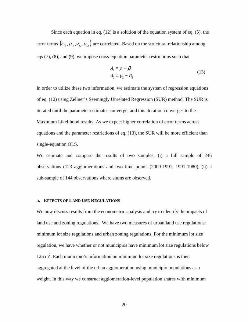
Since each equation in eq. (12) is a solution of the equation system of eq. (5), the

error terms ( )titititi ,,,, ,,, υνµε are correlated. Based on the structural relationship among

eqs (7), (8), and (9), we impose cross-equation parameter restrictions such that

.222

111

βγλβγλ

−=−=

(13)

In order to utilize these two information, we estimate the system of regression equations

of eq. (12) using Zellner’s Seemingly Unrelated Regression (SUR) method. The SUR is

iterated until the parameter estimates converge, and this iteration converges to the

Maximum Likelihood results. As we expect higher correlation of error terms across

equations and the parameter restrictions of eq. (13), the SUR will be more efficient than

single-equation OLS.

We estimate and compare the results of two samples: (i) a full sample of 246

observations (123 agglomerations and two time points (2000-1991, 1991-1980), (ii) a

sub-sample of 144 observations where slums are observed.

5. EFFECTS OF LAND USE REGULATIONS

We now discuss results from the econometric analysis and try to identify the impacts of

land use and zoning regulations. We have two measures of urban land use regulations:

minimum lot size regulations and urban zoning regulations. For the minimum lot size

regulation, we have whether or not municipios have minimum lot size regulations below

125 m2. Each municipio’s information on minimum lot size regulations is then

aggregated at the level of the urban agglomeration using municipio populations as a

weight. In this way we construct agglomeration-level population shares with minimum

21

lot size regulations below 125 m2. For the urban zoning regulations, we construct

agglomeration-level data in the same way: aggregating municipio-level information on

the existence of urban zoning regulations into agglomeration levels using municipio

populations as weights.

A caveat is that we only observe urban land regulations in 1999. This is a

potential problem as we don’t have much time variance in the data. However, we are

interested in seeing if cities have moved away from the federally mandated 1979 lot size

regulation and developed zoning plans. In this context, our land use regulation variables

will reasonably capture local regulatory environments and their impacts on migration and

formal housing market.

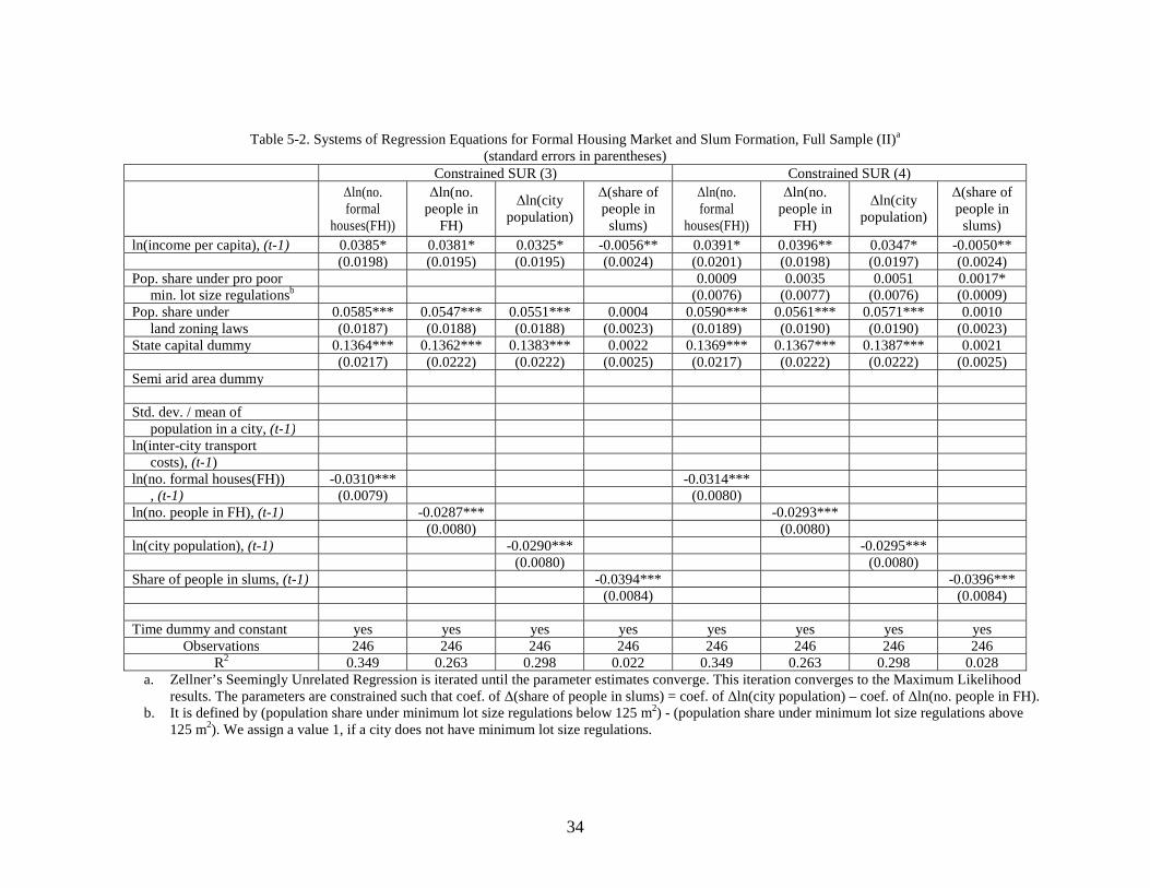
We first look at the results from the full sample (246 observations) estimation. We

add to each equation (i) base period endowments that may capture mean reversion, and

(ii) a dummy for state capitals, which could be more favored with resource allocation and

investment in unobserved amenities. Tables 5-1 to 5-3 show constrained SUR results in

various specifications. In all specifications we find that in general, cities who have

instituted regulations to lower land subdivision sizes from the Federal specification of

125 m2 have experienced higher rates of slum formation. In the tables, this variable is

called “pro-poor minimum lot size regulations” and is calculated by taking the difference

between the population share under minimum lot size regulations below 125 m2 and that

of above 125 m2. We assign a value of 1 if a city does not have minimum lot size

regulations. We find that regulations that reduce minimum lot sizes increase migration as

well as formal house residents, even though both are not statistically significant.

However, as the resulting city population growth is higher than formal housing supply

22

growth, we observe a statistically significant increase in slum formation. While it would

be interesting to find out the reasons why some cities enacted pro poor subdivision

standards, we do not have information on the political economy of the land management

process to comment on this. We however checked and could not find evidence to support

systematic selection bias arising from differences in incomes or city size.

This empirical result that pro-poor land use regulations encourage immigration of

the poor and indeed increase slum formation is consistent with the finding of Glaeser et

al.(2000) who find that urbanization of poverty in the US can be attributed to central city

governments’ favoring the poor relative to suburban governments.

The effects of general purpose urban zoning regulations are quite different from

those of pro-poor minimum lot size regulations. Urban zoning regulations are expected to

improve urban land use efficiency, in particular of formal (housing) sector. Adequate

planning facilitates timely infrastructure investment and large scale urban development.

Efficient land use also improves urban productivity. In all specifications, we observe

urban zoning regulations to have positive and statistically significant effects on the

growth of the formal housing market and city population. As the effects on city

population and formal housing supply are of the same magnitudes, their opposite effects

on slum formation are cancelled out. While urban zoning regulations increase city growth

and have beneficial effects on formal housing sector, zoning regulations do not have

distinct effects on slum formation.

Now we turn to the other interesting findings. In all specifications we observe

very strong mean reversions. Base period endowments of the formal housing market

(formal housing stock and residents), city population, and therefore slum formation have

23

negative and statistically significant (at the 1% levels) effects on their subsequent growth.

It suggests either mean reversions from random external shocks or some convergence, or

both.

State capitals display higher growth of the formal housing market and city

population than other cities. It may reflect disproportionate state resource allocation

biased towards state capitals, in particular with respect to infrastructure and public

services. However, the beneficial effects of formal housing market growth are cancelled

out by the same magnitude of city population growth. In sum, there is no net effect on

slum formation.

We also find that cities with higher initial per capita incomes have lower slum

formation. In all specifications, the estimated effects of initial per capita incomes on

formal housing market growth (formal housing stock and residents) and population

growth are positive and statistically significant. However as the formal housing market

growth is much higher than population growth, we observe in all specifications a negative

and statistically significant (at the 5% levels) initial income effect on slum formation. For

example in specification 4 of Table 5-2, a 10% increase in base period’s per capita

income raises city population growth rate by 0.35%p (over 10 years) and formal house

residents growth rate by 0.40%p (over 10 years). Therefore, it decreases slum shares by

0.05%p (over 10 years). The income effect dominates the substitution effect, and

economic growth reduces slum formation, thus confirming eq. (11) for Brazil that

0ln

_

1

>∂

∆∂

−tY

shareslum.

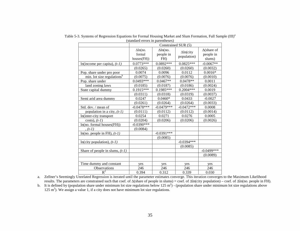
Finally, we experiment the effects of other local characteristics (in the base

period) which may influence city growth, formal housing supply and therefore slum

24

formation.11 We measure geographical dispersion of city population by the ratio of the

standard deviation to the mean of city population at MCA levels. We find that more

dispersed cities experience smaller increases in formal housing supply and lower

population growth. Infrastructure and public service provision will cost more in dispersed

cities, and therefore they will experience difficulty in increasing formal housing stock

which requires adequate basic public services. However, there is no net effect on slum

formation as two opposite effects on city population and formal housing supply are

cancelled out. Being located in semi-arid areas and inter-city transport costs do not have

statistically significant effects on slum formation when we control for other determinants

listed above.12

Sub-Sample: Robustness test

Cities that already have slum dwellings may function differently from those

which do not have slums. In this regard, we restrict the sample and re-estimate only for

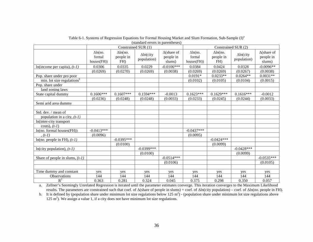
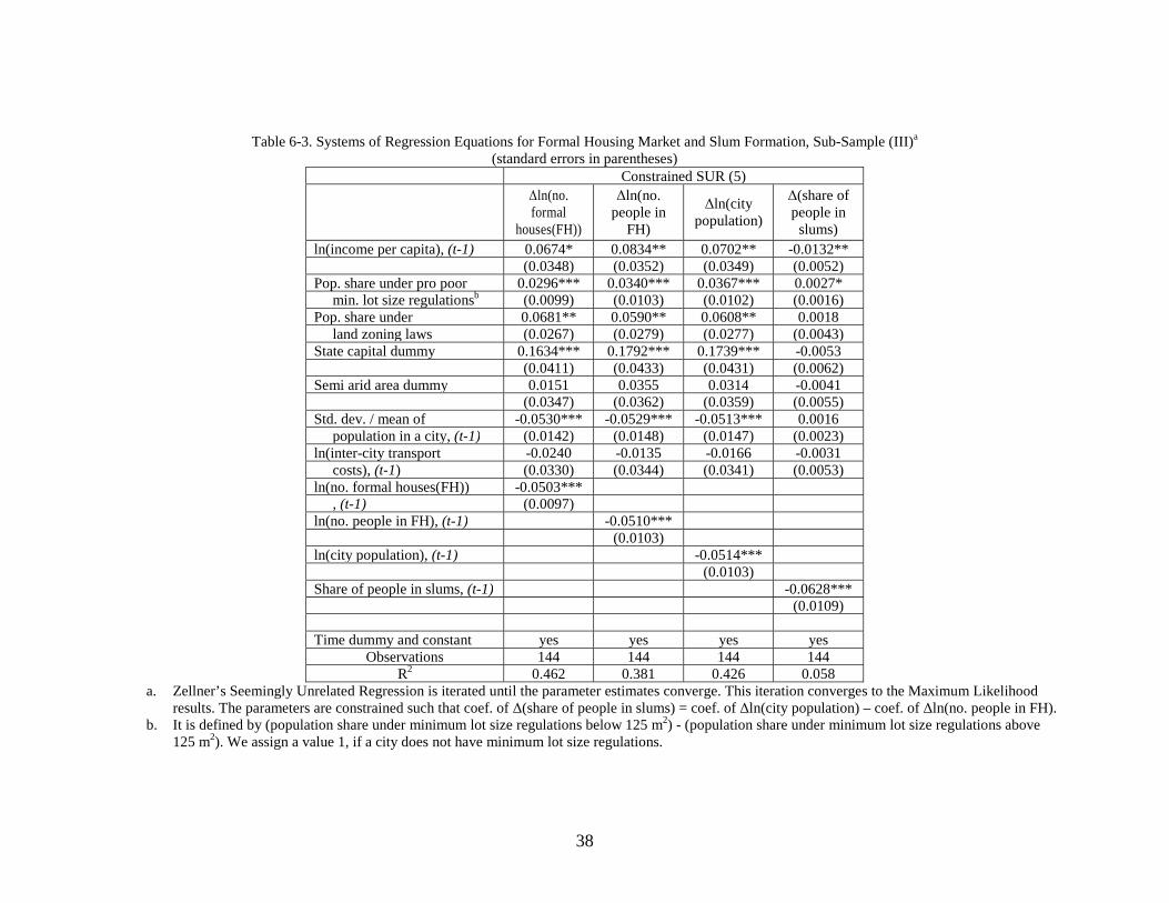
the cities which have slums. This reduces sample size to 144 observations. Tables 6-1 to

6-3 show constrained SUR results for this sub-sample. Basically we observe very similar

results.

There are strong mean reversions and favoritism towards state capitals. Cities

with higher initial per capita incomes have lower slum growth in all specifications.13 Pro

poor minimum lot size regulations increase both migration and formal house residents,

now both become statistically significant. As city population growth dominates formal

11 Glaeser at al. (2000) shows that urbanization of poverty in the US would be a result of better access to public transportation services in central cities. 12 The definition of inter-city transport costs is in Appendix A. 13 While the combined effects on slum formation is negative and statistically significant, the separate effects on city population and formal housing market become statistically insignificant.

25

housing supply growth, we observe statistically significant and positive effect of pro-poor

minimum lot size regulations on slum formation. Urban zoning regulations raise the

growth of the formal housing market and city population at the same magnitude, and

therefore there is no net effect on slum formation. Again, other local characteristics, such

as geographical dispersion of city population, semi-arid areas, and inter-city transport

costs, have similar effects as in the full sample. These sub-sample results confirm that

there is no statistical difference between the full and sub-samples.

6. SUMMARY AND CONCLUSIONS

In this paper, we examine the effects of land use and zoning regulations on

housing supply and slum formation across Brazilian cities between 1980 and 2000. We

find very low price elasticities of housing supply in the Brazilian formal housing market,

which limits formal housing supply adjustments in response to demand increases, and is

linked with growth of informal settlements. The imputed Brazilian formal housing supply

elasticity is similar to those in Malaysia and South Korea, which have been regarded to

have restrictive regulatory environments.

We also find that land use regulations that manage densities – in particular,

minimum lot size regulations, have important effects in terms of housing supply and slum

formation. Contrary to conventional wisdom, lowering minimum lot size regulations do

not lead to a reduction in slum formation. If city population growth were exogenous and

households did not consider local regulations in their migration and residential location

26

decisions, then lowering minimum lot sizes would allow cities to accommodate more

residents into formal housing developments – and unambiguously reduce slum formation.

However, when we consider that regulations are a part of household migration

and residential choice decisions, the exact effects of lowering regulatory standards are not

obvious. In fact, our model suggests that the net effect of land regulations depends on the

extent to which new formal housing supply absorbs demand, both from current informal

sector residents and population growth induced by lowering regulations. Our estimation

strategy considers both effects, and we find that cities that lowered minimum lot size

regulations from the Federal stipulation of 125 m2 experienced higher growth in the

formal housing stock. However, this was also accompanied by higher population growth

from migration, and the resulting city population growth was higher than the formal

housing supply response, exacerbating the slum formation problem.

Local innovations that increase access to land for the poor – such as flexible land

sub divisions – are welfare enhancing as they allow houses with different specifications

to be available in the market, thereby allowing low income residents to benefit from

services that meet their preferences (and affordability). However, if some cities offer

improved access to land compared to their peers, these cities are likely to

disproportionately attract (poor) migrants. If the induced population growth is higher than

formal housing supply adjustment, informality is likely to grow. Cities that absorb

migrants increase welfare – and in this context the challenge is to identify strategies that

increase formal housing supply relative to population growth. The econometric results

should not be viewed as a failure of flexible zoning to reduce slum formation. Rather, the

27

focus should be on identifying pre existing distortions in the land and housing market that

reduce the formal housing supply response to additional demand.

Two important issues for future research emerge from this analysis. First, to

understand why some cities deviated from the federally stipulated minimum lot

specification of 125 m2 to favor low income housing development. And second, to

identify sources of land and housing supply distortions that reduce the elasticity of formal

housing supply.

7. REFERENCES

Angel, S. (2000). Housing Policy Matters: A Global Analysis, Oxford University Press.

Da Mata, D., U. Deichmann, V. Henderson, S. Lall, and H. Wang (2005). “Determinants of City Growth in Brazil,” World Bank Policy Research Working Paper #3723.

Fernandes, E. (1997), “Access to Urban Land and Housing in Brazil: Three Degrees of Illegality,” Lincoln Institute of Land Policy Working Paper #WP97EF1.

Fix, M., P. Arantes, and G. Tanaka (2003), “The Case of Sao Paulo,” in UN-Habitat, The Challenge of Slums: Global Report on Human Settlements 2003, Earthscan, London.

Glaeser, E., M. Kahn, and J. Rappaport (2000). “Why Do the Poor Live in Cities?” NBER Working Paper #7636.

Glaeser, E. and J. Gyourko (2002), “The Impact of Zoning on Housing Affordability,” NBER Working Paper #8835.

Glaeser, E., J. Gyourko, and R. Saks (2005a). “Urban Growth and Housing Supply,” NBER Working Paper #11097.

Glaeser, E., J. Gyourko, and R. Saks (2005b), “Why Have Housing Prices Gone Up?” The American Economic Review, 95, AEA Papers and Proceedings, 329-333.

Green, R., S. Malpezzi, and S. Mayo (2005), “Metropolitan-Specific Estimates of the Price Elasticity of Supply of Housing, and Their Sources,” The American Economic Review, 95, AEA Papers and Proceedings, 334-339.

Henderson, J.V. (1985). Economic Theory and the Cities, Academic Press, Inc.

IPEA, IBGE, and UNICAMP (2002), Configuração Atual e Tendêncies da Rede Urbana, Serie Configuração Atual e Tendêncies da Rede Urbana, Instituto de Pesquisa Econômica Aplicada, Instituto Brasileiro de Geografia e Estatistica, Universidade Estadual de Campinas, Brasilia.

Krueckeberg, D. and K. Paulsen (2000), “Urban Land Tenure Policies in Brazil, South Africa, and India: An Assessment of the Issues,” Lincoln Institute Research Report #LP00Z26.

28

Malpezzi, S. and S. Mayo (1987), “The Demand for Housing in Developing Countries: Empirical Estimates from Household Data,” Economic Development and Cultural Change, 35, 687-721.

Malpezzi, S. and S. Mayo (1997), “Getting Housing Incentives Right: A Case Study of the Effects of Regulation, Taxes, and Subsidies on Housing Supply in Malaysia,” Land Economics, 73, 372-391.

Malpezzi, S. and D. Maclennan (2001), “The Long-Run Price Elasticity of Supply of New Residential Construction in the United States and the United Kingdom,” Journal of Housing Economics, 10, 278-306.

Mayer, C. and C. Somerville (2000), “Residential Construction: Using the Urban Growth Model to Estimate Housing Supply,” Journal of Urban Economics, 48, 85-109.

Quigley, J. and S. Raphael (2005), “Regulation and the High Cost of Housing in California,” The American Economic Review, 95, AEA Papers and Proceedings, 323-328.

Saks, R. (2005), “Job Creation and Housing Construction: Constraints on Metropolitan Area Employment Growth” FEDs Working Paper #2005-49.

Serra, M., D. Dowall, D. Motta, and M. Donovan (2004), “Urban Land Markets and Urban Land Development: An Examination of Three Brazilian Cities: Brasília, Curitiba and Recife,” Working Paper at Institute of Urban and Regional Development, University of California at Berkeley #2004-03.

Sivam, A. (2002), “Constraints Affecting the Efficiency of the Urban Residential Land Market in Developing Countries: A Case Study of India,” Habitat International, 26, 523-537.

Smolka, M. and C. De Cesare (2006), “Property Taxation and Informality: Challenges for Latin America,” Land Lines, 18 (3).

Soule, N. (1999), “Forms of Protection of the Right to Housing and the Combat of Forced Eviction in Brazil,” Paper presented at the International Research Group on Law and Urban Space/Centre for Applied Legal Studies Workshop on Facing the Paradox: Redefining Property in the Age of Liberalization and Privatization, Johannesburg, 29-30 July.

United Nations (2003), World Urbanization Prospects.

United Nations (2005), The Millennium Development Goals Report 2005, New York.

World Bank (2002). Brazil Progressive Low-Income Housing: Alternatives for the Poor, Report No. 22032 BR.

World Bank (2006). Urban Strategy.

29

Table 1. City Growth a

1980 1991 2000 units in cities population (a) 62,390,783 80,885,091 96,951,317 housing units (b) 14,012,484 20,564,931 27,126,584 slum dwellers (c) 2,224,164 4,084,051 5,775,890 slum units (d) 476,292 943,667 1,488,779 share to total (%)b population 52.42 55.09 57.10 housing units 55.40 58.03 59.61 slum dwellers 97.45 91.11 88.38 slum units 97.56 91.72 89.53 annual growth rate (%) population 3.69 2.36 2.01 housing units 4.93 3.49 3.08 slum dwellers .. 5.52 3.85 slum units .. 6.22 5.07 slum shares in cities (%) population (c/a) 3.56 5.05 5.96 housing units (d/b) 3.40 4.59 5.49

a. For 123 agglomerations covering 447 MCAs (Minimum Comparable Areas). b. Share to total is the ratio of 123 urban agglomerations (447 MCAs) over the total 3,659 MCAs.

30

Table 2. Slum Formation by City Sizes, 2000a

city sizeb no.

cities

no. population, a (thousand)

no. slum dwellers, b (thousand)

Slum share (b/a, %)

no. housing stock,

(thousand)

no. formal houses / no. total houses

(%) 5.301 ≤ pop/mean (4.178M ≤ pop)

4 39,095.6 3,566.4 9.12 11,409.6 91.78

1.340 ≤ pop/mean < 5.301 (1.056M ≤ pop < 4.178M)

11 25,260.3 1,583.4 6.27 6,786.9 94.18

0.812 ≤ pop/mean < 1.340 (640K ≤ pop < 1.056M)

14 11,682.8 302.5 2.59 3,160.4 97.62

0.469 ≤ pop/mean < 0.812 (370K ≤ pop < 640K)

17 7,699.9 154.7 2.01 2,098.7 98.20

0.256 ≤ pop/mean < 0.469 (202K ≤ pop < 370K)

20 5,879.1 81.1 1.38 1,624.3 98.80

pop/mean < 0.256 (pop < 202K)

57 7,333.5 87.8 1.20 2,046.8 98.86

Total 123 96,951.3 5,775.9 5.96 27,126.6 94.51

a. Population, slum dwellers, and housing stock are the sums of city figures in each groups. b. “pop” refers to city population, and “mean” the average city population.

31

Table 3. The Formal Housing Market

Dependent variable: (1) (2)

∆ln(no. formal houses) OLS OLS

∆ln(income per capita) 0.020 0.051***

(0.016) (0.020)

∆ln(no. people in formal Houses) 0.958*** 0.948***

(0.017) (0.019)

time dummies Yes Yes

Observations 246 144

(no. cities) (123 cities) (72 cities)

Adjusted R2 0.945 0.956

Test for heteroskedasticitya

( )12χ 1.60 0.99

(p-value) (0.206) (0.321) *** significant at 1% level; ** significant at 5% level; * significant at 10% level.

a. We report the result of Breusch-Pagan / Cook-Weisberg test for heteroskedasticity.

32

Table 4. The Imputed Price Elasticity of Housing Supply

Assumption on demand elasticity

Formal housing stock growth, Table 3

Malpezzi and Mayo (1997) Malpezzi and

Maclennan (2001)

1α 2α Column (1) Column (2) Malaysi

a South Korea

Thailand US,

postwar UK,

postwar

-0.5 0.5 0.021 0.057 0.000a 0.000a ∞b 6.079 0.000a

-0.5 1.0 0.010 0.027 0.068 0.000a ∞b 12.658 0.488

-0.5 1.5 0.007 0.018 0.352 0.174 ∞b 19.237 0.982

-1.0 0.5 0.042 0.114 0.000a 0.000a ∞b 5.579 0.000a

-1.0 1.0 0.020 0.054 0.000a 0.000a ∞b 12.158 0.000a

-1.0 1.5 0.014 0.035 0.000a 0.000a ∞b 18.737 0.482

a. The imputed supply price elasticity was negative, and set equal to zero. b. The point estimate of the reduced form coefficient was negative, and interpreted as perfectly elastic.

33

Table 5-1. Systems of Regression Equations for Formal Housing Market and Slum Formation, Full Sample (I)a (standard errors in parentheses)

Constrained SUR (1) Constrained SUR (2)

∆ln(no. formal

houses(FH))

∆ln(no. people in

FH)

∆ln(city population)

∆(share of people in

slums)

∆ln(no. formal

houses(FH))

∆ln(no. people in

FH)



slums) ln(income per capita), (t-1) 0.0451** 0.0450** 0.0395** -0.0056** 0.0443** 0.0453** 0.0404** -0.0048** (0.0201) (0.0197) (0.0196) (0.0024) (0.0204) (0.0200) (0.0199) (0.0024) Pop. share under pro poor -0.0026 0.0001 0.0017 0.0016* min. lot size regulationsb (0.0077) (0.0077) (0.0077) (0.0009) Pop. share under land zoning laws State capital dummy 0.1366*** 0.1360*** 0.1382*** 0.0021 0.1372*** 0.1367*** 0.1387*** 0.0020 (0.0221) (0.0225) (0.0225) (0.0025) (0.0221) (0.0225) (0.0226) (0.0025) Semi arid area dummy Std. dev. / mean of population in a city, (t-1) ln(inter-city transport costs), (t-1) ln(no. formal houses(FH)) -0.0269*** -0.0271*** , (t-1) (0.0080) (0.0080) ln(no. people in FH), (t-1) -0.0249*** -0.0253*** (0.0080) (0.0080) ln(city population), (t-1) -0.0251*** -0.0255*** (0.0080) (0.0080) Share of people in slums, (t-1) -0.0356*** -0.0356*** (0.0084) (0.0084) Time dummy and constant yes yes yes Yes yes yes yes yes

Observations 246 246 246 246 246 246 246 246 R2 0.329 0.245 0.277 0.022 0.329 0.245 0.277 0.026

a. Zellner’s Seemingly Unrelated Regression is iterated until the parameter estimates converge. This iteration converges to the Maximum Likelihood results. The parameters are constrained such that coef. of ∆(share of people in slums) = coef. of ∆ln(city population) – coef. of ∆ln(no. people in FH).

b. It is defined by (population share under minimum lot size regulations below 125 m2) - (population share under minimum lot size regulations above 125 m2). We assign a value 1, if a city does not have minimum lot size regulations.

34

Table 5-2. Systems of Regression Equations for Formal Housing Market and Slum Formation, Full Sample (II)a (standard errors in parentheses)


∆ln(no. formal

houses(FH))

∆ln(no. people in

FH)



slums)

∆ln(no. formal

houses(FH))

∆ln(no. people in

FH)



slums) ln(income per capita), (t-1) 0.0385* 0.0381* 0.0325* -0.0056** 0.0391* 0.0396** 0.0347* -0.0050** (0.0198) (0.0195) (0.0195) (0.0024) (0.0201) (0.0198) (0.0197) (0.0024) Pop. share under pro poor 0.0009 0.0035 0.0051 0.0017* min. lot size regulationsb (0.0076) (0.0077) (0.0076) (0.0009) Pop. share under 0.0585*** 0.0547*** 0.0551*** 0.0004 0.0590*** 0.0561*** 0.0571*** 0.0010 land zoning laws (0.0187) (0.0188) (0.0188) (0.0023) (0.0189) (0.0190) (0.0190) (0.0023) State capital dummy 0.1364*** 0.1362*** 0.1383*** 0.0022 0.1369*** 0.1367*** 0.1387*** 0.0021 (0.0217) (0.0222) (0.0222) (0.0025) (0.0217) (0.0222) (0.0222) (0.0025) Semi arid area dummy Std. dev. / mean of population in a city, (t-1) ln(inter-city transport costs), (t-1) ln(no. formal houses(FH)) -0.0310*** -0.0314*** , (t-1) (0.0079) (0.0080) ln(no. people in FH), (t-1) -0.0287*** -0.0293*** (0.0080) (0.0080) ln(city population), (t-1) -0.0290*** -0.0295*** (0.0080) (0.0080) Share of people in slums, (t-1) -0.0394*** -0.0396*** (0.0084) (0.0084) Time dummy and constant yes yes yes yes yes yes yes yes

Observations 246 246 246 246 246 246 246 246 R2 0.349 0.263 0.298 0.022 0.349 0.263 0.298 0.028



35

Table 5-3. Systems of Regression Equations for Formal Housing Market and Slum Formation, Full Sample (III)a (standard errors in parentheses)

Constrained SUR (5)

∆ln(no. formal

houses(FH))

∆ln(no. people in

FH)



slums) ln(income per capita), (t-1) 0.0773*** 0.0892*** 0.0825*** -0.0067** (0.0265) (0.0260) (0.0260) (0.0032) Pop. share under pro poor 0.0074 0.0096 0.0112 0.0016* min. lot size regulationsb (0.0075) (0.0076) (0.0076) (0.0010) Pop. share under 0.0493*** 0.0467** 0.0478** 0.0011 land zoning laws (0.0185) (0.0187) (0.0186) (0.0024) State capital dummy 0.1915*** 0.1985*** 0.2004*** 0.0019 (0.0311) (0.0318) (0.0319) (0.0037) Semi arid area dummy 0.0247 0.0460* 0.0433 -0.0027 (0.0261) (0.0264) (0.0264) (0.0033) Std. dev. / mean of -0.0478*** -0.0479*** -0.0472*** 0.0008 population in a city, (t-1) (0.0111) (0.0112) (0.0112) (0.0014) ln(inter-city transport 0.0254 0.0271 0.0276 0.0005 costs), (t-1) (0.0204) (0.0206) (0.0206) (0.0026) ln(no. formal houses(FH)) -0.0390*** , (t-1) (0.0084) ln(no. people in FH), (t-1) -0.0391*** (0.0085) ln(city population), (t-1) -0.0394*** (0.0085) Share of people in slums, (t-1) -0.0499*** (0.0089) Time dummy and constant yes yes yes yes

Observations 246 246 246 246 R2 0.394 0.312 0.339 0.030



36

Table 6-1. Systems of Regression Equations for Formal Housing Market and Slum Formation, Sub-Sample (I)a (standard errors in parentheses)


∆ln(no. formal

houses(FH))

∆ln(no. people in

FH)



slums)

∆ln(no. formal

houses(FH))

∆ln(no. people in

FH)



slums) ln(income per capita), (t-1) 0.0306 0.0335 0.0229 -0.0106*** 0.0384 0.0424 0.0328 -0.0096** (0.0269) (0.0270) (0.0269) (0.0038) (0.0269) (0.0269) (0.0267) (0.0038) Pop. share under pro poor 0.0191* 0.0233** 0.0264** 0.0031** min. lot size regulationsb (0.0102) (0.0105) (0.0104) (0.0015) Pop. share under land zoning laws State capital dummy 0.1606*** 0.1607*** 0.1594*** -0.0013 0.1623*** 0.1629*** 0.1616*** -0.0012 (0.0236) (0.0248) (0.0248) (0.0033) (0.0233) (0.0245) (0.0244) (0.0033) Semi arid area dummy Std. dev. / mean of population in a city, (t-1) ln(inter-city transport costs), (t-1) ln(no. formal houses(FH)) -0.0413*** -0.0437*** , (t-1) (0.0096) (0.0095) ln(no. people in FH), (t-1) -0.0395*** -0.0424*** (0.0100) (0.0099) ln(city population), (t-1) -0.0399*** -0.0428*** (0.0100) (0.0099) Share of people in slums, (t-1) -0.0514*** -0.0535*** (0.0106) (0.0105) Time dummy and constant yes yes yes yes yes yes yes yes

Observations 144 144 144 144 144 144 144 144 R2 0.363 0.281 0.324 0.045 0.375 0.298 0.350 0.057



37

Table 6-2. Systems of Regression Equations for Formal Housing Market and Slum Formation, Sub-Sample (II)a (standard errors in parentheses)


∆ln(no. formal

houses(FH))

∆ln(no. people in

FH)



slums)

∆ln(no. formal

houses(FH))

∆ln(no. people in

FH)



slums) ln(income per capita), (t-1) 0.0259 0.0288 0.0182 -0.0106*** 0.0342 0.0378 0.0281 -0.0097** (0.0265) (0.0268) (0.0267) (0.0038) (0.0264) (0.0266) (0.0263) (0.0038) Pop. share under pro poor 0.0218** 0.0259** 0.0290*** 0.0031** min. lot size regulationsb (0.0100) (0.0104) (0.0103) (0.0016) Pop. share under 0.0657** 0.0579** 0.0580** 0.0001 0.0722*** 0.0655** 0.0665** 0.0009 land zoning laws (0.0281) (0.0292) (0.0291) (0.0043) (0.0278) (0.0288) (0.0285) (0.0043) State capital dummy 0.1580*** 0.1587*** 0.1574*** -0.0012 0.1595*** 0.1606*** 0.1593*** -0.0013 (0.0232) (0.0246) (0.0245) (0.0033) (0.0228) (0.0241) (0.0240) (0.0033) Semi arid area dummy Std. dev. / mean of population in a city, (t-1) ln(inter-city transport costs), (t-1) ln(no. formal houses(FH)) -0.0447*** -0.0477*** , (t-1) (0.0096) (0.0095) ln(no. people in FH), (t-1) -0.0426*** -0.0461*** (0.0100) (0.0099) ln(city population), (t-1) -0.0430*** -0.0464*** (0.0100) (0.0099) Share of people in slums, (t-1) -0.0545*** -0.0572*** (0.0106) (0.0105) Time dummy and constant yes yes yes yes yes yes yes yes

Observations 144 144 144 144 144 144 144 144 R2 0.380 0.293 0.339 0.046 0.395 0.314 0.370 0.058



38

Table 6-3. Systems of Regression Equations for Formal Housing Market and Slum Formation, Sub-Sample (III)a (standard errors in parentheses)

Constrained SUR (5)

∆ln(no. formal

houses(FH))

∆ln(no. people in

FH)



slums) ln(income per capita), (t-1) 0.0674* 0.0834** 0.0702** -0.0132** (0.0348) (0.0352) (0.0349) (0.0052) Pop. share under pro poor 0.0296*** 0.0340*** 0.0367*** 0.0027* min. lot size regulationsb (0.0099) (0.0103) (0.0102) (0.0016) Pop. share under 0.0681** 0.0590** 0.0608** 0.0018 land zoning laws (0.0267) (0.0279) (0.0277) (0.0043) State capital dummy 0.1634*** 0.1792*** 0.1739*** -0.0053 (0.0411) (0.0433) (0.0431) (0.0062) Semi arid area dummy 0.0151 0.0355 0.0314 -0.0041 (0.0347) (0.0362) (0.0359) (0.0055) Std. dev. / mean of -0.0530*** -0.0529*** -0.0513*** 0.0016 population in a city, (t-1) (0.0142) (0.0148) (0.0147) (0.0023) ln(inter-city transport -0.0240 -0.0135 -0.0166 -0.0031 costs), (t-1) (0.0330) (0.0344) (0.0341) (0.0053) ln(no. formal houses(FH)) -0.0503*** , (t-1) (0.0097) ln(no. people in FH), (t-1) -0.0510*** (0.0103) ln(city population), (t-1) -0.0514*** (0.0103) Share of people in slums, (t-1) -0.0628*** (0.0109) Time dummy and constant yes yes yes yes

Observations 144 144 144 144 R2 0.462 0.381 0.426 0.058



39

Figure 1. The Top 10 Cities with the Highest Rates of Slum Formation between 1980 and 2000

40

Figure 2. Slum Dweller Growth and City Population Growth between 1980 and 2000

-.1

0.1

.2gr

_nsl

um

0 .02 .04 .06pop growth rate, annual:1980-2000

slum dweller growth rate, annual:1980-2000 Fitted values

gr_nslum vs. gr_n

OLS:

)20/1(

1980

2000

_

_ln

dwellersslum

dwellersslum = -2.11*

)20/1(

1980

2000ln

pop

pop + 0.109

(-1.45) (2.92) N=35, adj R2 = 0.031, t-values in parentheses.

41

Figure 3. Slum Formation and Formal Housing Stock Growth between 1980 and 2000

-.1

0.1

.2gr

_nsl

um

.02 .04 .06 .08formal house growth rate, annual:1980-2000

slum dweller growth rate, annual:1980-2000 Fitted values

gr_nslum vs. gr_fh

OLS:

)20/1(

1980

2000

_

_ln

dwellersslum

dwellersslum = -2.99*

)20/1(

1980

2000

_

_ln

housesformal

housesformal + 0.163

(-2.32) (3.48) N=35, adj R2 = 0.114, t-values in parentheses.

42

Figure 4. Housing Supply Elasticity and Slum Formation.

(a) a city of inelastic housing supply (b) a city of elastic housing supply

∆FNie P P

∆FNe

FH FH

P0

FHie

P0+∆P

FHie+∆FHie FHe FHe+∆FHe

DFH0 DFH1 DFH0

DFH1 SieFH

SeFH

43

Appendix A. Data sources and definitions

The data used for the analysis are produced through a joint research program between

IPEA, Brasilia and the World Bank. There is no official statistical or administrative entity in

Brazil that reflects the concept of a city or urban agglomeration that is appropriate for economic

analysis. Socioeconomic data in Brazil tend to be available for municipios, the main

administrative level for local policy implementation and management. Municipios, however, vary

in size. In 2000, Sao Paulo municipio had a population of more than ten million, while many

other municipios had only a few thousand residents. Furthermore, many functional

agglomerations consist of a number of municipios, and the boundaries of these units change over

time.

Our analysis therefore adapts the concepts of agglomerations from a comprehensive

urban study by IPEA, IBGE and UNICAMP (2002), and modifies this classification slightly by

also including smaller municipios to existing agglomerations if their population exceeded 75,000

population and more than 75 percent of its residents lived in urban areas in 1991, or if they were

completely enclosed by an agglomeration. To create a consistent panel of agglomerations, we

therefore used the Minimum Comparable Area (MCA) concept as implemented by IPEA

researchers. MCAs group municipios in each of the census years so that their boundaries do not

change during the study period. All data have then been aggregated to match these MCAs. The

resulting data set represents 123 urban agglomerations that consist of a total of 447 MCAs. Based

on matching between municipios and agglomerations listed above, municipio-level data are

aggregated to agglomeration levels using population or geographical area sizes as weights.

The sources of population, housing, and slum data are the Brazilian Bureau of Statistics

(IBGE) Population and Housing Censuses of 1980, 1991 and 2000. Per capita income figures are

compiled from monthly data, deflated to 2000 Real (R$).

Sources of land use regulations and semi-arid dummy?

44

The transportation costs between municipalities and the nearest State capitals come from

Professor Newton De Castro at the Federal University of Rio De Janeiro, and available at

www.ipeadata.gov.br. We divide that variable by distance from the city to the state capital to get

a city specific measure of local unit transport costs, defined as “intercity transport costs”. We use

1980 value for years 1980 and 1990, and 1995 value for 2000.

45

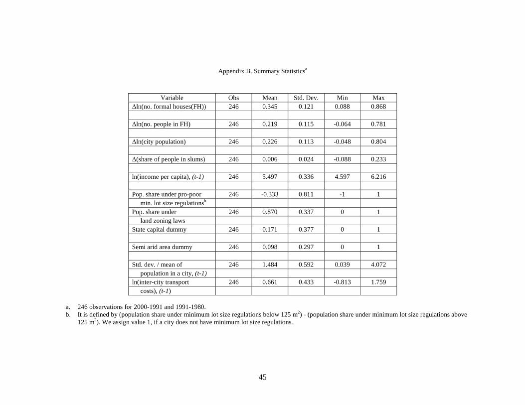
Appendix B. Summary Statisticsa

Variable Obs Mean Std. Dev. Min Max ∆ln(no. formal houses(FH)) 246 0.345 0.121 0.088 0.868 ∆ln(no. people in FH) 246 0.219 0.115 -0.064 0.781 ∆ln(city population) 246 0.226 0.113 -0.048 0.804 ∆(share of people in slums) 246 0.006 0.024 -0.088 0.233 ln(income per capita), (t-1) 246 5.497 0.336 4.597 6.216

Pop. share under pro-poor 246 -0.333 0.811 -1 1 min. lot size regulationsb Pop. share under 246 0.870 0.337 0 1 land zoning laws State capital dummy 246 0.171 0.377 0 1 Semi arid area dummy 246 0.098 0.297 0 1 Std. dev. / mean of 246 1.484 0.592 0.039 4.072 population in a city, (t-1) ln(inter-city transport 246 0.661 0.433 -0.813 1.759 costs), (t-1)

a. 246 observations for 2000-1991 and 1991-1980. b. It is defined by (population share under minimum lot size regulations below 125 m2) - (population share under minimum lot size regulations above

125 m2). We assign value 1, if a city does not have minimum lot size regulations.

46

Appendix C. Correlation Coefficientsa

∆ln(no. formal

houses(FH))

∆ln(no. people in

FH)



slums)

ln(income per capita),

(t-1)

Pop. share under

generous min. lot size regulationsb

Pop. share under land zoning laws

State capital dummy

Semi arid area

dummy

Std. dev. / mean of

population in a city,(t-1)

ln(inter-city transport

costs), (t-1)

∆ln(no. formal houses(FH)) 1 ∆ln(no. people in FH) 0.964 1 ∆ln(city population) 0.944 0.975 1 ∆(share of people in slums) -0.146 -0.171 0.054 1 ln(income per capita), (t-1) 0.156 0.166 0.162 -0.031 1

Pop. share under generous -0.031 -0.019 -0.002 0.081 -0.161 1 min. lot size regulationsb Pop. share under 0.168 0.173 0.185 0.040 0.199 -0.161 1 land zoning laws State capital dummy 0.267 0.287 0.306 0.064 0.151 0.017 0.176 1 Semi arid area dummy -0.107 -0.089 -0.086 0.022 -0.586 0.169 -0.117 -0.149 1 Std. dev. / mean of -0.084 -0.081 -0.062 0.089 0.179 0.174 -0.054 0.268 -0.031 1 population in a city, (t-1) ln(inter-city transport -0.151 -0.180 -0.175 0.031 -0.152 -0.041 -0.036 -0.695 0.081 -0.077 1 costs), (t-1)

a. 246 observations for 2000-1991 and 1991-1980. b. It is defined by (population share under minimum lot size regulations below 125 m2) - (population share under minimum lot size regulations above

125 m2). We assign value 1, if a city does not have minimum lot size regulations

do urban land regulations influence slum formation?...

Documents