Munich Personal RePEc Archive

Do Speculative Bubbles Migrate in the

Chinese Stock Market?

He, Qing and Qian, Zongxin and Fei, Zhe and Chong,

Terence Tai Leung

Renmin University of China, Renmin University of China, Renmin

University of China, The Chinese University of Hong Kong and

Nanjing University

1 December 2016

Online at https://mpra.ub.uni-muenchen.de/80575/

MPRA Paper No. 80575, posted 03 Aug 2017 23:10 UTC

1

Do Speculative Bubbles Migrate in the Chinese

Stock Market?

Qing HE1, China Financial Policy Research Center & School of Finance,

Renmin University of China

Zongxin QIAN, International Monetary Institute & School of Finance,

Renmin University of China

Zhe FEI, School of Finance, Renmin University of China

Terence Tai-Leung CHONG2,

Department of Economics and Lau Chor Tak Institute of Global Economics and

Finance, The Chinese University of Hong Kong,

Department of International Economics and Trade, Nanjing University

1/12/16

Abstract

In this paper, a duration dependence test for speculative bubbles in the Chinese stock

market is developed. It is found that bubbles in the aggregate stock price existed

before the split share reform. After the reform, we observe the phenomenon of bubble

migration across industries. In particular, bubbles migrate from the

telecommunications industry to the health care industry. Moreover, we find that

monetary policy used to have a significant impact on the bubble size before the

reform but the impact diminished after the reform.

Keywords: Survival analysis; Speculative bubbles; Non-tradable shares reform

JEL Classifications: G12

1. This research is supported by the MOE Project of Key Research Institute of Humanities and Social Sciences at

Universities (16JJD790056), National Natural Science Foundation of China (71402181), and Fundamental

Research Funds for the Central Universities, and the Research Funds of Renmin University of China (13XNJ003).

All remaining errors are ours. 2 Corresponding Author: Terence Tai-Leung Chong, Department of Economics, The Chinese University

of Hong Kong, Shatin, N.T., Hong Kong. Email: chong2064@cuhk.edu.hk. Phone (852)39431614.

Webpage: http://www.cuhk.edu.hk/eco/staff/tlchong/tlchong3.htm.

2

1. Introduction

The 2008 financial crisis triggered by the burst of the subprime mortgage market

bubble has had a profound impact on the global economy (Brueckner et al., 2012).

The Chinese stock market experiences similar boom and bust cycles. The market rose

by approximately 400% from 2001 to 2007, but experienced a bust in 2008 in which

the Shanghai composite index dropped by more than 75.74%. Whether this is a

normal market cycle or a burst of bubbles has not yet been fully addressed. Given

China’s crucial role as a global economic power, the understanding of equity bubbles

and the boom and bust cycle of this market therefore becomes increasingly important

for international investors and policy makers.

A number of studies in the literature have attempted to detect bubbles in equity

markets (Hamilton, 1986; West, 1988; Fukuta, 2002). A strand of literature regards

equity bubble as the deviation of actual price from the fundamentals, and develops a

variance bounds test to detect the bubbles, e.g., Shiller (1981) and LeRoy and Porter

(1981). However, the variance bounds test relies on linearity assumption that relates

all the observations to the value of prior observations. Gurkaynak (2008) suggests that

bubbles demonstrate nonlinear patterns in return, and one cannot attribute the

violation of the variance bound in data to the existence of a bubble. Another strand of

the literature examines the statistical attributes of equity bubbles. For example,

Blanchard and Watson (1983) develop autocorrelation and kurtosis tests for equity

bubbles. Evans (1987) detects bubbles in the foreign exchange market using a

skewness test. Diba and Grossman (1988) implement both unit root and co-integration

tests to detect equity bubbles. However, these statistical features can also be driven by

fundamental values and made them difficult to conclusively test equity bubbles. To

incorporate the nonlinearity patterns on equity return, McQueen and Thorley (1994)

3

develop a duration dependence test for bubbles, by allowing the probability of ending

a bubble to depend on the length of positive or negative abnormal returns. The

duration dependence test is more closely related to bubbles than other measures such

as autocorrelation and skewness (McQueen and Thorley, 1994; Lunde and

Timmermann, 2004). This method has been widely used to detect rational speculative

bubbles in both developed and developing countries, such as, Asian countries (Chan et

al., 1998), Malaysia (Mokhtar and Hassan, 2006), Thailand (Jirasakuldech et al., 2008)

and more recently US (Wan and Wong, 2015).

In this paper, we apply the duration dependence test to examine bubbles in the

Chinese stock market. Zhang (2008) also applies the duration dependence test in the

Chinese stock market for a sample period of 1991-2001. However, He does not

consider the important link between structural changes at the industry level and

dynamic changes in bubbles at the aggregate level. Moreover, the relationship

between monetary policy and bubbles is yet to be studied. Our study addresses the

above issues by investigating bubbles in stock prices at the industry level, and the

impact of the split share reform on the dynamics of bubbles. Thus, our study has

valuable policy implications on both capital market and monetary policy in an

emerging market economy such as China.

One of the most important capital market reforms in China has been the alleged

“split share reform” of listed enterprises. From the beginning, a so-called “split share

structure” was established to maintain the State’s dominant role in corporate operation

in the Chinese stock market. Most government-owned shares, together with shares

issued to other investors before IPOs (legal person shares), were strictly prohibited

from trading in the secondary markets. Before 2005, only approximately one-third of

the shares in listed firms were freely tradable. There were a plenty of speculative

4

transactions, as stock prices are not driven by their fundamental values (He et al.,

2017). In addition, corporate managers have less incentive to improve firms' value as

they do not benefit from an increase in share prices. In April 2005, the China

Securities Regulatory Commission (CSRC) published Guidance Notes on the split

share reform of Listed Companies. The reform was aimed to convert all non-tradable

shares into legitimate tradable shares in the secondary market. It improves market

liquidity and overall operational efficiency of listed firms, since all shares are priced

at market values. Thus, the split share reform provides us a unique opportunity to

examine the relationship between trading restrictions and speculative bubbles.

Consistent with Zhang (2008), our results show that bubbles exist in China's stock

market. However, the contribution of a bubble to the overall stock price is moderate

after the split share reform. This suggests that the release of trading restrictions help

mitigate speculative bubbles. Looking at the speculative bubbles at the industry level,

we find a migration of bubbles from the telecommunications sector to the health care

sector after the reform. In addition, we find that monetary policy tools are effective in

suppressing bubbles in particular for the period prior to the split share reform.

Harman and Zuehlke (2004) suggest that duration dependence tests for

speculative bubbles are sensitive to model specifications. To check the robustness, we

repeat our empirical studies across various specifications. Our empirical results

remain robust to the method correcting for discrete observation, the use of

equally-weighted and value-weighted portfolios, and the use of weekly versus

monthly stock returns.

The rest of the paper proceeds as follows. Section 2 briefly introduces the

duration dependence test. Section 3 reports the empirical results. The impact of

monetary policy on bubbles is discussed. We also conduct a variety of specifications

5

to examine the robustness of our results. The conclusion is presented in Section 4.

2. The Duration Dependence Test

Following McQueen and Thorley (1994), we assume that the price of an asset is

equal to its intrinsic value plus a bubble, i.e.:

*

tt tp p b (1)

where is the bubble, 1 1[ ] (1 )t t t tE b r b ,and *

1 1

/ (1 )

i

t t t i t j

i j

p E d r

is the fundamental value, t id is the dividend, 1tr is the required rate of return.

Bubbles can grow and burst; more specifically, we define

1 0

1

0

(1 ) / (1 ) / ,

, 1

t t

t

r b a with probabilityb

a with probability

(2)

Bubbles grow with probability , which compensates the loss of the investors

when bubbles burst (with probability 1 . When bubbles burst, the price reverts to

the initial price with a small initial bubble value, 0a . McQueen and Thorley (1994)

show that, for a bubble to exist, the probability of a negative abnormal return

conditional on a sequence of prior positive abnormal returns decreases with the

duration of the prior period with positive abnormal returns. The duration dependence

test is based on the logistic transformation of the log of the length of the prior run of

positive abnormal returns:

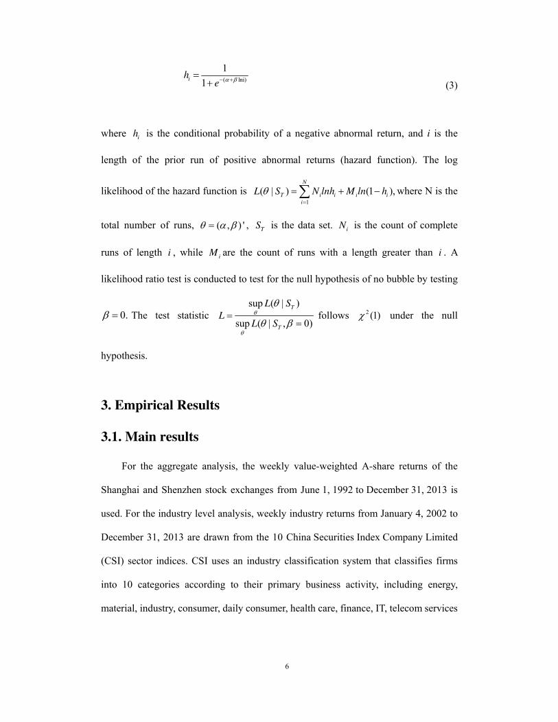
6

( lni)

1

1ih

e (3)

where ih is the conditional probability of a negative abnormal return, and i is the

length of the prior run of positive abnormal returns (hazard function). The log

likelihood of the hazard function is 1

( | ) (1 ),

N

T i i i i

i

L S N lnh M ln h where N is the

total number of runs, ( , ) ' , TS is the data set.

iN is the count of complete

runs of length i , while iM are the count of runs with a length greater than i . A

likelihood ratio test is conducted to test for the null hypothesis of no bubble by testing

0. The test statistic

sup ( | )

sup ( | , 0)

T

T

L S

LL S

follows 2 (1) under the null

hypothesis.

3. Empirical Results

3.1. Main results

For the aggregate analysis, the weekly value-weighted A-share returns of the

Shanghai and Shenzhen stock exchanges from June 1, 1992 to December 31, 2013 is

used. For the industry level analysis, weekly industry returns from January 4, 2002 to

December 31, 2013 are drawn from the 10 China Securities Index Company Limited

(CSI) sector indices. CSI uses an industry classification system that classifies firms

into 10 categories according to their primary business activity, including energy,

material, industry, consumer, daily consumer, health care, finance, IT, telecom services

7

and utilities.3 As China implemented the split share reform in April, 2005, we split the

sample into the prior and post-reform period, with the first week of April 2005 as the

cut-off point. All data are retrieved from the CSMAR database.

Figure 1 shows the weekly continuously compounded nominal returns for the

Chinese comprehensive A-share stock market from June 1992 to December 2013. It

shows that the Chinese stock market is quite volatile over the past two decades. The

compounded stock returns vary with a range from 0.5 to 1.5 over the period 1992-2005.

The stock returns increased almost fivefold from 2005 to 2007. During the global

financial crisis around 2008, stock market fell by more than 60%. Even though China

implemented a number of stimulus policies, e.g. a lower interest rate and bank reserve

ratio4, the stock market did not recover by the end of 2013.

Figure 1.Weekly continuously compounded nominal returns (Equally-weighted)

3 The China Securities Index (CSI) Company Limited is a joint venture between the Shanghai Stock Exchanges

and the Shenzhen Stock Exchange. It provides the creation and management of indices and index-related services.

To measure the stock performance of different industries, the company launched 10 industry indices on January 4,

2002. 4 To offset adverse global economic conditions, the Chinese government launched a CNY 4-trillion

stimulus plan on Nov. 9, 2008, to boost domestic demand by providing extra liquidity.

8

To conduct the duration dependence test, we first calculate the abnormal returns

and divide them into two states (positive versus negative). McQueen and Thorley

(1994) estimate a multi-factor model and use the residuals as abnormal returns. The

factors in their model include the term spread between AAA bonds and government

bonds, yield and dividend. As the dividend distribution system in China is

under-developed, it is inappropriate to use the dividend to measure the fundamentals of

the Chinese stock market (He and Rui, 2016). Lunde and Timmermann (2004) discuss

the impact of inflation on the drift of nominal stock prices. Thus, we also include a

proxy of inflation in our regression model. Note that the volatility of weekly stock

returns is serially correlated, which will affect the duration distribution. To account for

the effect of volatility clustering, we employ Engle and Lee (1999)’s generalized

autoregressive conditional heteroscedasticity model with an ARCH-in-mean effect

(C-GARCH) 5

. Following Mcqueen and Thorley (1994), we allow the C-GARCH

model with lagged returns of up to three orders6. More specifically, we use the

following model to calculate the abnormal returns in the Chinese stock market:

2

1 1 1 1 2 2 3 3 , (0, ),t t t t t t t t tR IFLA R R R N

2 2 2

1 1 1 1( ) ( ),t t t t t t

q q q

2 2

1 1 1( ) ( )t t t tq q (4)

where tR is the compounded weekly returns on the equally-weighted portfolios.7

IFLA is the consumer price index (CPI) inflation rate. The weekly inflation rate is

5 In unreported results, we conduct an ARCH test and find conditional heteroscedasticity in weekly stock return

series. 6 We obtain similar results by using a GARCH-in-mean model with lag returns up to three orders. 7 Engle and Lee (1999) show that under mild assumptions, the variance equation of model (4) can be rewritten as

an equation with five coefficients, which identifies the five underlying parameters.

9

calculated in the same way as Lunde and Timmermann (2004)8.

t is the conditional

standard deviation, tq is the temporary component of t and is the permanent

component of t .

Table 1 summarizes the duration statistics of aggregate and industrial abnormal

returns and the duration dependence tests of equation (3) for full sample9. The result

from Panel A of Table 1 suggests that there is a bubble in the aggregate stock price.

The results of the industrial-level analysis in Panel B suggest that the bubble

originates from the health care sector. This result is consistent with market

expectations. By 2013, the price-earnings ratio of the health care sector has exceeded

36, nearly 4 times the price-earnings ratio of the market. It reflects that the risk of

innovations, such as new medicine and new medical apparatus, in this sector is

underestimated.

Table 1 Summary Statistics of duration

Panel A Summary Statistics of durations for aggregate market

Run

Length

Positive Negative

Death

Total 238

Survival Hazard

Rate

Death

Total 239

Survival Hazard

Rate

1 133 105 0.5588 108 131 0.4519

2 41 64 0.3905 61 70 0.4656

3 23 41 0.3594 19 51 0.2714

4 17 24 0.4146 20 31 0.3922

5 10 14 0.4167 12 19 0.3871

6 1 13 0.0714 5 14 0.2632

7 6 7 0.4615 8 6 0.5714

8 3 4 0.4286 3 3 0.5000

9 2 2 0.5000 2 1 0.6667

10 1 1 0.5000 0 1 0.0000

11 1 0 1.0000 1 0 1.0000

Log-Logistic Test

-0.1400 (0.3402) 0.2045 (0.4625)

8 The monthly CPI is converted into weekly inflation rates by solving the weekly inflation rate such that the weekly

price index grows smoothly and at the same rate between subsequent values of the monthly CPI. 9 It should be noted that in equation (3) refers to population probability, whereas the h(i) refers to the sample

probability used in the likelihood tests.

10

0.4651 (0.0901) 0.1667 (0.4962) 2 (1) 2.7250 (0.0901) 0.4631 (0.4962)

Panel B Summary Statistics of durations for industrial returns

Run Energy Material Industry Consumer Daily-C Health Finance Info. Telecom Utility

1 0.508 0.465 0.503 0.516 0.536 0.519 0.522 0.485 0.475 0.514

2 0.424 0.400 0.473 0.495 0.592 0.568 0.535 0.460 0.495 0.528

3 0.434 0.350 0.449 0.435 0.655 0.632 0.550 0.444 0.521 0.524

4 0.467 0.333 0.407 0.500 0.600 0.500 0.556 0.633 0.522 0.450

5 0.563 0.423 0.563 0.615 0.750 0.571 0.625 0.727 0.636 0.545

6 0.286 0.533 0.571 0.600 1.000 1.000 0.333 0.667 0.750 1.000

7 0.400 0.429 0.333 1.000 0.500 1.000 1.000

8 0.333 0.500 0.500 1.000

9 0.500 0.500 1.000

10 1.000 1.000

Log-Logistic Test

0.206 0.163 0.099 0.038 -0.373 0.680 -0.071 -0.229 -0.259 -0.120

(0.80) (0.52) (0.88) (0.95) (0.90) (0.01) (0.98) (0.36) (0.67) (0.86)

Obs. 187 187 187 188 153 183 180 194 181 183

The run length i represents that the number of weeks for which a series of abnormal returns lasts. The

abnormal returns are errors estimated by the C-GARCH model in equation (4). The sample hazard rate

is calculated by ( ) i

i i

Nh i

M N

, where iN

represents the number of death, and iM represents

the number of survival. The parameter of α, β is estimated by | ∑ 1 , where TS is the data set, ( lni)1/1

ih e . P-values are in the parentheses.

The split share reform started in April 2005. To account for the potential market

structural change caused by this reform, we estimate the model and conduct duration

test of equation (3) for subsample periods. The results are summarized in Table 2.

Table2. Summary Statistics of durations for subperiods

Run

Length

Positive Negative

Death

Total 152

Survival Hazard

Rate

Death

Total 152

Survival Hazard

Rate

Panel A: Pre-reform period

1 89 63 0.5855 67 85 0.4408

2 28 35 0.4444 38 47 0.4471

3 13 22 0.3714 10 37 0.2128

4 11 11 0.5 16 21 0.4324

5 5 6 0.4545 7 14 0.3333

6 0 6 0 5 9 0.3571

7 4 2 0.6667 7 2 0.7778

11

9 1 1 0.5 1 1 0.5

11 1 0 1 1 0 1

Log-Logistic Test

-0.2812 (0.4007) 0.2810 (0.3777)

0.4692 (0.0828) 0.1172 (0.6559) 2 (1) 3.0094 (0.0828) 0.1986 (0.6559)

Panel B: Post-reform period

1 44 42 0.5116 41 46 0.4713

2 13 29 0.3095 23 23 0.5000

3 10 19 0.3448 9 14 0.3913

4 6 13 0.3158 4 10 0.2857

5 5 8 0.3846 5 5 0.5000

6 1 7 0.1250 0 5 0

7 2 5 0.2857 1 4 0.2000

8 3 2 0.6000 3 1 0.7500

9 1 1 0.5000 1 0 1

10 1 0 1

Log-Logistic Test

0.0903 (0.7411) 0.0604 (0.8994)

0.4374 (0.1153) 0.2747 (0.4374)

2 (1) 2.4805 (0.1153) 0.6030 (0.4374)

The run length i represents that the number of weeks for which a series of abnormal returns lasts. The

abnormal returns are errors estimated by the C-GARCH model in equation (4). The sample hazard rate

is calculated by ( ) i

i i

Nh i

M N

, where iN

represents the number of death, and iM represents

the number of survival. The parameters α, β are estimated by maximizing the log-likelihood | ∑ 1 . P-values are in the parentheses.

Before the reform, there were 152 duration spells for both positive and negative

abnormal returns. After the reform, there are 86 observations of duration spells for

positive abnormal returns and 87 observations of duration spells for negative

abnormal returns. Statistics for the hazard rate are also reported. Note that the hazard

rate of durations drops initially and rises thereafter. It is evident that beyond a certain

duration, the existence of bubbles is highly dependent on the length of the duration.

After nine spells, a bubble bursts. The results of the LR tests are reported in the last

three rows of Table 2. Before the split share reform, the null of 0 conditional on

positive abnormal returns is rejected at the 10% level, which shows the presence of

bubbles and their dependence on durations; after the reform, the p-value for the null

12

of 0 conditional on positive abnormal returns is 0.1153. The “no bubble”

hypothesis cannot be rejected at the conventional confidence level. Thus, the

aggregate analysis suggests that the reform was effective in eliminating the bubble.

Figure 1 shows that Chinese stock market index increased fourfold and dropped at

the same extent from 2006 to 2008. Someone may suspect that there is a bubble in the

post-split share reform period. A possible explanation is that split share reform is

effective in mitigating the conflicts between tradable and non-tradable shareholders,

and improves the corporate operation efficiency. A large number of studies have

shown that the reform has a strong positive influence on the corporate performance.

(Firth et al., 2010; Liao et al., 2014, He et al., 2017). Corporate managers are more

willing to serve for the benefits of shareholders so as to increase firm’s operating and

market performance. The rise of stock market index is more likely to be driven by

better economic fundamentals rather than speculative bubbles. The financial crisis

around 2008 led to a global economic recession. Stock market fell by more than 60%,

as investors expected a slowing down of Chinese economy due to this adverse external

shock.

Figure2.a Survival Function and confidence intervals for aggregate market

13

Figure 2.b Survival Function and confidence intervals before the reform

Figure 2.c Survival Function and confidence intervals after the reform

Upper 95% CI

Lower 95% CI

Survival Curve

Su

rviv

al Pro

bab

ility

Duration

Duration

Su

rviv

al Pro

bab

ility

14

Figure3.a Cumulative Hazard Rate and confidence intervals for aggregate market

02

46

8

Cum

ula

tive

Hazard

0 5 10

Duration

Upper 95% CI

Hazard Rate

Lower 95% CI

Upper 95% CI

Lower 95% CI

Survival Curve

Surv

ival P

robab

ility

Duration

Cu

mulativ

e Hazard

Rate

Duration

15

Figure 3.b Cumulative Hazard Rate and confidence intervals before the reform

Figure 3.c Cumulative Hazard Rate and confidence intervals after the reform

Figures 2a, 2b and 2c depict the survival function and its 95% confidence

intervals. Figures 3a, 3b and 3c depict the cumulative hazard rate function and its 95%

Upper 95% CI

Lower 95% CI

Hazard Rate

Cu

mu

lative H

azard R

ate

Duration

Upper 95% CI

Lower 95% CI

Hazard Rate

Cu

mulativ

e Hazard

Rate

Duration

16

confidence intervals. All confidence intervals are calculated using a likelihood ratio

test.

Table 3.Summary Statistics of durations for industrial returns in sub-periods

Run Energy Material Industry Consumer Daily-C Health Finance Info. Telecom Utility

Panel A: Pre-reform period

1 0.522 0.443 0.514 0.554 0.694 0.594 0.576 0.529 0.624 0.524

2 0.438 0.359 0.500 0.552 0.727 0.577 0.571 0.545 0.467 0.467

3 0.500 0.320 0.471 0.462 1.000 0.455 0.583 0.467 0.515 0.375

4 0.444 0.176 0.444 0.571 0.333 0.600 0.500 0.700 0.300

5 0.600 0.257 0.800 0.333 0.500 1.000 0.500 1.000 0.571

6 0.500 0.444 1.000 0.500 1.000 0.500 1.000

7 1.000 0.500 1.000 1.000

8 0.333

9 0.500

10 1.000

Log-Logistic Test

0.028 0.213 -0.113 0.101 -0.820 0.240 -0.186 0.018 -0.420 0.125

(0.17) (0.28) (0.88) (0.96) (0.53) (0.87) (0.89) (0.99) (0.09) (0.82)

Obs. 67 70 70 65 36 64 66 70 63 63

Panel B: Post-reform period

1 0.500 0.479 0.496 0.496 0.487 0.579 0.491 0.460 0.449 0.508

2 0.417 0.426 0.458 0.468 0.567 0.565 0.517 0.418 0.462 0.559

3 0.400 0.371 0.438 0.424 0.615 0.400 0.536 0.436 0.486 0.615

4 0.476 0.455 0.389 0.474 0.600 0.625 0.538 0.682 0.500 0.600

5 0.545 0.500 0.455 0.700 0.750 0.667 0.500 0.857 0.556 0.500

6 0.200 0.667 0.500 0.667 1.000 1.000 0.333 1.000 0.750 1.000

7 0.250 0.500 0.333 1.000 0.500 1.000

8 0.333 1.000 0.500 1.000

9 0.500 1.000

10 1.000

Log-Logistic Test

0.198 0.013 0.134 -0.078 -0.499 -0.657 -0.108 -0.374 -0.256 -0.354

(0.34) (0.97) (0.87) (0.85) (0.83) (0.05) (0.95) (0.14) (0.71) (0.84)

Obs. 120 117 117 123 117 119 114 124 118 120

The run length i represents that the number of weeks for which a series of abnormal returns lasts. The abnormal

returns are errors estimated by the C-GARCH model in equation (4). The sample hazard rate is

calculated by ( ) i

i i

Nh i

M N

, where iN

represents the number of death, and iM represents the

17

number of survival. The parameter of the log-logistic test is estimated by | ∑ 1 . P-values are in the parentheses.

Note from Table 3 that there is duration dependence in the telecommunications

industry (p-value = 0.09) prior to the reform; Thereafter, the health care industry

shows significant duration dependence (p-value = 0.05). Therefore, our findings

suggest that the bubble does not completely disappear after the reform. Instead, it

migrates from the telecommunications industry to the health care industry.

3.2. Tests for Differences in Duration

McQueen and Thorley (1994) suggest that duration dependence should only exist

in runs of positive abnormal returns when there are bubbles. In this section, two basic

models suggested by Lunde and Timmermann (2004) are introduced for testing the

differences in samples of duration spells. As there is no closed-form solution for any

of the duration models, we apply non-parametric two-sample tests to compare the

duration dependence between the subsamples (Hollander and Wolfe, 1999). Three

assumptions are made:

1) the number of duration spells is i iN M N , iN represents the number of

deaths, and iM represents the number of survival;

2) the two sample spaces are 1 2, ,..., PX X X and 1 2, ,..., PY Y Y ;

3) X and Y are mutually independent and respectively subject to the continuous

distribution functions F and G.

We first apply the Wilcoxon, Mann and Whitney test for the following null

hypothesis:

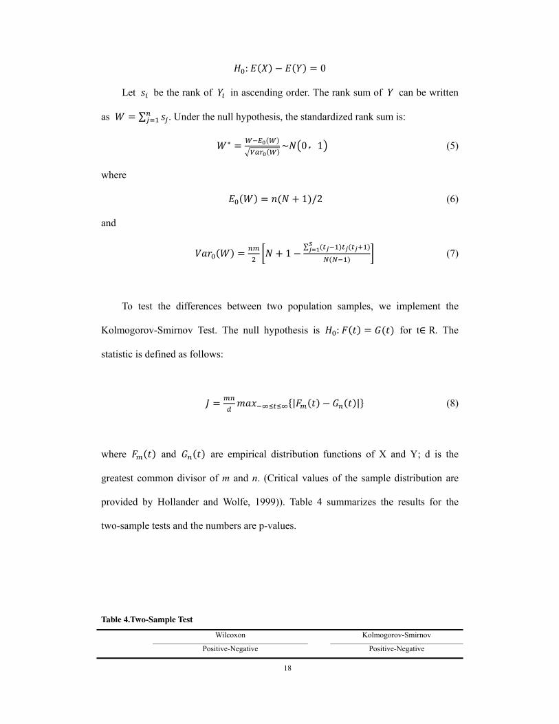
18

: 0

Let be the rank of in ascending order. The rank sum of can be written

as ∑ . Under the null hypothesis, the standardized rank sum is:

∗ ~ 0，1 (5)

where 1 /2 (6)

and

1 ∑ (7)

To test the differences between two population samples, we implement the

Kolmogorov-Smirnov Test. The null hypothesis is : for t∈ R. The

statistic is defined as follows:

| | (8)

where and are empirical distribution functions of X and Y; d is the

greatest common divisor of m and n. (Critical values of the sample distribution are

provided by Hollander and Wolfe, 1999)). Table 4 summarizes the results for the

two-sample tests and the numbers are p-values.

Table 4.Two-Sample Test

Wilcoxon Kolmogorov-Smirnov

Positive-Negative Positive-Negative

19

Before 0.0102 0.065

After 0.8708 0.964

Before-After Before-After

Positive 0.1189 0.494

Negative 0.4593 0.806

This table reports the two-sample test results (p-values) by comparing the sample of duration spells of

positive abnormal returns with the sample of duration spells of negative abnormal returns (Equation 8).

The tests are carried out for both periods before and after the reform. P-values<0.1 are highlighted in

boldface.

Based on the two-sample test of positive and negative abnormal returns in the

prior reform period, noticeable differences can be observed between the positive

abnormal return rate and the negative abnormal return rate; after the reform, we find

insignificant difference between these two samples. This result is consistent with our

previous finding that the contribution of bubbles to the aggregate stock index has

significantly been reduced after the reform. It is evident that the split share reform has

suppressed the speculative bubbles.

3.3. The Impact of the Interest Rate on Bubbles

While the increase of interest rate generally has a negative impact on stock returns,

there is little analysis of its influence on bubbles in the Chinese stock market. To

examine this, the influences of interest rate (I) and its change (ΔI) on bubbles are

analyzed under four distributional assumptions, namely, the exponential distribution,

the Weibull distribution, the Gompertz distribution and the Cox proportional model.

The weekly risk-free interest rate is collected from CSMAR, which is the one-year

deposit rate announced by the central bank10

. Table 5 reports the regression results for

10 We also use the repo rate as alternative measure of risk-free interest rate. It turns out that our results remain

qualitatively unchanged.

20

the hazard rate under the four distributional assumptions.

Table 5. Regression for Interest Rate

(1) (2) (3) (4)

COEFFICIENT Exponential Weibull Gompertz Cox

Whole

I 0.0112* 0.0163 0.0124 0.0086

(0.006) (0.010) (0.008) (0.054) ∆I 0.368*** 0.547*** 0.438*** 0.318**

(0.140) (0.177) (0.167) (0.142)

Cons. -0.892*** -1.400*** -1.071***

(0.090) (0.158) (0.136)

Obs. 236 236 236 236

Before

I 0.0134 0.0218 0.0169 0.0123

(0.01) (0.02) (0.01) (0.01) ∆I 0.265*** 0.373*** 0.304*** 0.247***

(0.08) (0.11) (0.10) (0.08)

Cons. -0.853*** -1.408*** -1.080***

(0.12) (0.19) (0.15)

Obs. 141 141 141 141

After

I 0.0285 0.049 0.0421 0.0323

(0.077) (0.12) (0.098) (0.07) ∆I -1.415 -2.448 -1.744 -1.106

(1.06) (1.6) (1.28) (0.91)

Cons. -0.937** -1.532** -1.238**

(0.44) (0.66) (0.55)

Obs. 95 95 95 95

The exponential regression is exp ∆ , the Weibull regression

is ∗ exp ∆ , the Gompertz regression is ∗ exp exp ∆ , the cox regression is 0 ∗exp ∆ , where h is the hazard rate. Robust Standard Deviations are in the parentheses

and *** denotes p value <0.01, ** denotes p value <0.05 * denotes p value <0.1

For the whole period, an increase in the interest rate leads to a significant

increase in the hazard rate and a decrease in bubble duration. This indicates that the

interest rate policy played a role in suppressing bubbles. This result is robust under

four different specifications.

21

Looking at the periods prior to and after the split share reform, we find a

significant difference. Before the reform, an increase in the interest rate leads to a

significant increase in the hazard rate and a decrease in bubble duration. These

indicate that the interest rate policy was effective in suppressing bubbles. In contrast,

this effect no longer exists in the post-reform period. A possible explanation is that in

the post-reform period, there were expectations of RMB appreciation. These

expectations, together with an inflexible exchange rate regime, led to a huge stock of

foreign reserve. The accumulation of foreign reserve led to excess liquidity supply,

which added pressure to asset price appreciation. Much of the monetary tightening in

this period was to offset the impact of the excess liquidity supply. Therefore, its

impact could be weaker than the prior-reform periods in which the foreign reserve-led

excess liquidity problem was not a major concern.

3.4. Robustness tests

Thus far, our primary results are based on weekly returns on the

equally-weighted portfolios from June 1992 to December 2013, with the abnormal

return estimated from equation (4). To check if our duration test is sensitive to the

estimation method and the use of the weekly or monthly returns (Harman and Zuehlke,

2004), we repeat the test on a variety of specifications. For each specification, we

report the results for both equally- and value- weighted portfolios.

In case I-IV, alternative methods are used to estimate positive and negative

abnormal returns. In Case I-III, we use continuous interval and discrete Weibull

models, respectively, to examine the sensitivity of our results to the method of

correcting for discrete observation of continuous duration. The runs of positive

abnormal returns still show a significant duration dependence, and the no-bubble

22

hypothesis is rejected at the traditional level of significance. The runs of negative

abnormal returns still fail to reject the no-bubble hypothesis. These results are robust

to the use of equally-weighted or value-weighted portfolio series.

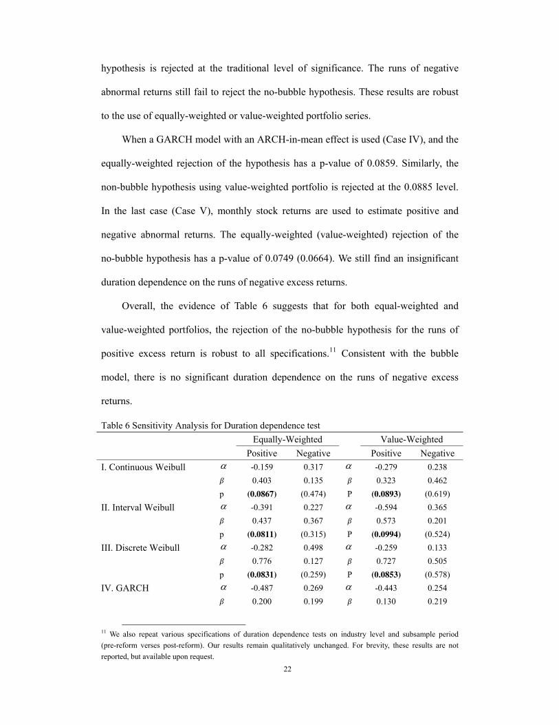
When a GARCH model with an ARCH-in-mean effect is used (Case IV), and the

equally-weighted rejection of the hypothesis has a p-value of 0.0859. Similarly, the

non-bubble hypothesis using value-weighted portfolio is rejected at the 0.0885 level.

In the last case (Case V), monthly stock returns are used to estimate positive and

negative abnormal returns. The equally-weighted (value-weighted) rejection of the

no-bubble hypothesis has a p-value of 0.0749 (0.0664). We still find an insignificant

duration dependence on the runs of negative excess returns.

Overall, the evidence of Table 6 suggests that for both equal-weighted and

value-weighted portfolios, the rejection of the no-bubble hypothesis for the runs of

positive excess return is robust to all specifications.11

Consistent with the bubble

model, there is no significant duration dependence on the runs of negative excess

returns.

Table 6 Sensitivity Analysis for Duration dependence test

Equally-Weighted Value-Weighted

Positive Negative Positive Negative

I. Continuous Weibull -0.159 0.317 -0.279 0.238

0.403 0.135 0.323 0.462

p (0.0867) (0.474) P (0.0893) (0.619)

II. Interval Weibull -0.391 0.227 -0.594 0.365

0.437 0.367 0.573 0.201

p (0.0811) (0.315) P (0.0994) (0.524)

III. Discrete Weibull -0.282 0.498 -0.259 0.133

0.776 0.127 0.727 0.505

p (0.0831) (0.259) P (0.0853) (0.578)

IV. GARCH -0.487 0.269 -0.443 0.254

0.200 0.199 0.130 0.219

11 We also repeat various specifications of duration dependence tests on industry level and subsample period

(pre-reform verses post-reform). Our results remain qualitatively unchanged. For brevity, these results are not

reported, but available upon request.

23

p (0.0859) (0.248) P (0.0885) (0.571)

V. Monthly return -0.198 -0.180 -0.484 -0.221

0.628 0.780 0.494 0.758

p (0.0749) (0.442) P (0.0664) (0.783)

Notes: In Case I-III, The parameter of α, β is estimated by continuous, interval and discrete Weibull

models as specified in Harman and Zuehlke, 2004. In Case IV, GARCH model with an ARCH-in-mean

effect instead of CGARCH is used to estimate the abnormal return. In Case V, monthly return instead

of weekly return is used. All cases include both equal-weighted and value-weighted portfolios. P-values

are in the parentheses.

4. Conclusion

The rising role of China as a major economic power has sparked the interest of

investors and researchers worldwide in understanding the behavior of its stock market.

In this paper, we implement a duration model to examine empirically the existence of

speculative bubbles in China's stock market. Evidence of the presence of bubbles is

found. Before the split share reform, the probability of bursting a bubble is shown to

have increased with the bubble duration. After the reform, the contribution of the

bubble component to the aggregate stock price reduces. Our result suggests that this

was caused by a structural change of the market at the industry level. Specifically,

bubbles existed in the telecommunications industry before the reform, but migrated to

the health care industry afterwards. Prior to the reform, there was segmentation of

tradable shares and non-tradable shares in the primary market. In the secondary

market, the non-payment of dividends also turns the market into a site for pursuing

highly speculative returns rather than value investments. As a result, it was difficult to

eliminate bubbles before the reform. Finally, our finding suggests that monetary

policy tools were effective in suppressing bubbles prior to the split shares reform, but

24

the effectiveness has dropped off significantly after the reform.

References

[1]. Blanchard, O. J., and Watson, M. W. (1983). “Bubbles, rational expectations and

financial markets” (No. 0945). National Bureau of Economic Research, Inc.

[2]. Brueckner, J. K., Calem, P. S., and Nakamura, L. I. (2012). “Subprime mortgages

and the housing bubble.” Journal of Urban Economics 71(2), pp. 230-243.

[3]. Chan, K., Mcqueen, G., and Thorley, S. (1998). “Are there rational speculative

bubbles in Asian stock markets?” Pacific-Basin Finance Journal 6(1-2), pp.125-151.

[4]. Dang, T. and He, Q., Bureaucrats as Successor CEOs (2016). BOFIT Discussion

Paper No. 13/2016.

[5]. Diba, B. T., and Grossman, H. I. (1988). “Explosive rational bubbles in stock

prices?” American Economic Review 78(3), pp. 520-530.

[6]. Engle, R. F., and Lee, G. J. (1999), "A Permanent and Transitory Component

Model of Stock Return Volatility," in Cointegration, Causality, and Forecasting: A

Festschrift in Honor of Clive, eds. W. J. Granger, R. F. Engle, and H. White, Oxford

University Press, pp.475-497.

[7]. Evans, D. S. (1987). “Tests of alternative theories of firm growth.” The Journal of

Political Economy 95(4), pp. 657-674.

[8]. Firth, M., C. Lin, and H. Zou (2010). Friend or foe? The role of state and mutual

fund ownership in the split share structure reform in China. Journal of Financial and

Quantitative Analysis, 45, 685–706.

[9]. Fukuta, Y. (2002). “A test for rational bubbles in stock prices.” Empirical

25

Economics 27(4), pp. 587-600.

[10]. Gürkaynak, R. S. (2008). “Econometric tests of asset price bubbles: Taking

Stock.” Journal of Economic Surveys 22(1), pp. 166-186.

[11]. Hamilton, J. D. (1986). “On testing for self-fulfilling speculative price bubbles.”

International Economic Review 27(3), pp. 545-552.

[12]. Harman, Y. S. and T. W. Zuehlke (2004). “Duration dependence testing for

speculative bubbles.” Journal of Economics and Finance 28(2), pp. 147–154.

[13]. He, Q., and Rui, O. (2016). “Ownership structure and insider trading: The

evidence from China.” Journal of Business Ethics 134(4), pp. 553-574.

[14]. He, Q. Xue, C., and Zhu, C. (2017) “Financial Development and the Patterns of

Industrial Specialization: the Evidence from China.” Review of Finance 21(4),

pp.1593-1638

[15]. Hollander, M., and Wolfe, D. A. (1999). Nonparametric Statistical Methods.

Wiley, Chichester.

[16]. Jirasakuldech, B., Emekter, R., and Rao, R. P. (2008). “Do Thai stock prices

deviate from fundamental values?” Pacific-Basin Finance Journal 16(3), pp. 298-315.

[17]. LeRoy, S. F., and Porter, R. D. (1981). “The present-value relation: Tests based

on implied variance bounds.” Econometrica 49(3), pp. 555-574.

[18]. Liao, L., B. Liu, and H. Wang (2014). China’s secondary privatization:

Perspectives from the Split-Share Structure Reform. Journal of Financial Economics,

113(3), 500–518.

[19]. Lunde, A., and Timmermann, A. (2004). “Duration dependence in stock prices:

An analysis of bull and bear markets.” Journal of Business and Economic

Statistics 22(3), pp. 253-273.

[20]. Mann, H. B., & Whitney, D. R. (1947). “On a test of whether one of two random

26

variables is stochastically larger than the other.” Annals of Mathematical

Statistics, 18(1), pp. 50-60.

[21]. McQueen, G., and Thorley, S. (1994). “Bubbles, stock returns, and duration

dependence.” Journal of Financial and Quantitative Analysis 29(3), pp. 379-401.

[22]. Mokhtar, S. H., and Hassan, T. (2006). “Detecting rational speculative bubbles

in the Malaysian stock market.” International Research Journal of Finance and

Economics 6, pp. 69-75.

[23]. Shiller, R. J. (1981). “Do stock prices move too much to be justified by

subsequent changes in dividends?”  American Economic Review 71(3), pp. 421-436.

[24]. Wang, M., and Wong, M. C. S. (2015). “Rational speculative bubbles in the US

stock market and political cycles.” Finance Research Letters 13, pp. 1-9.

[25]. West, K. D. (1988). “A specification test for speculative bubbles.” The

Quarterly Journal of Economics 102(3), pp. 553-580.

[26]. Zhang, B. (2008). “Duration dependence test for rational bubbles in Chinese

stock market.” Applied Economics Letters 15(8), pp. 635-639.