do poor kids get their fair share of school funding?do poor kids get their fair share of school...
TRANSCRIPT

Matthew M. Chingos and Kristin Blagg
May 2017
Funding elementary and secondary schools has always been a state and local affair in the
United States. Local governments provided more than 80 percent of school funding in the
1920s, but they have been roughly equal partners with state governments since the 1970s.
The federal government has never provided more than 13 percent of school funding, and
today it is responsible for less than 10 percent (figure 1).
School districts vary widely in their funding levels and sources. Essentially all districts receive at least
some funds from local sources, usually property taxes.1 Every state provides additional funds to school
districts based on a formula, with the details varying widely across states. States have many goals when it
comes to school funding, such as increasing funding statewide and providing targeted support for districts
that face higher costs, such as small districts in remote areas or those that serve many students with special
needs.
Redistributing funding across districts is a natural role for states to play, as they have the capacity to
collect taxes statewide and then apportion funding among local districts. One widely (but by no means
universally) shared goal among states is to target districts that serve higher percentages of students from
low-income families. By definition, these districts tend to have less wealth and thus less capacity to raise
local funds.
E D U C A T I O N P O L I C Y P R O G R A M
Do Poor Kids Get Their Fair Share
of School Funding?

2 D O P O O R K I D S G E T T H E I R F A I R S H A R E O F S C H O O L F U N D I N G ?
FIGURE 1
K–12 School Funding per Student
1919–2013 in 2015–16 dollars
Source: Digest of Education Statistics, 2016, table 235.10, https://nces.ed.gov/programs/digest/d16/tables/dt16_235.10.asp.
Most states have enacted policies aimed at narrowing differences in spending across districts,
increasing the resources available to districts that serve disadvantaged students, or both. Such school
finance reforms have been promulgated by courts and legislatures in at least 27 states since the early 1990s
(Lafortune, Rothstein, and Schanzenbach 2016).2 Recent research indicates that these efforts led to
increased test scores, educational attainment, and wages, especially among children from low-income
families (Jackson, Johnson, and Persico 2016; Lafortune, Rothstein, and Schanzenbach 2016).
Currently, 35 states have a provision in their formula that provides additional funding to districts
serving more low-income students.3 In theory, these provisions should make school funding more
progressive by spending more money on students from low-income families. But this depends on how
successful are states at counteracting local funding, which tends to be regressive.
In this report, we present new data on the progressivity of school district funding, focusing on the
degree to which the average low-income student attends districts that are better funded than districts the
average nonpoor student attends. We find that many states that have progressive funding formulas on
paper do not achieve this goal in practice, and that, in some states, the potential progressivity of school
funding is constrained by patterns of student sorting (segregation) by income.
$0
$2,000
$4,000
$6,000
$8,000
$10,000
$12,000
$14,000
1920 1930 1940 1950 1960 1970 1980 1990 2000 2010
Total Federal State Local

D O P O O R K I D S G E T T H E I R F A I R S H A R E O F S C H O O L F U N D I N G ? 3
A New Measure of Funding Progressivity
We propose a new measure of school funding progressivity that estimates average spending on all poor kids
(those from families below the federal poverty level) relative to nonpoor kids. Specifically, for each state, we
calculate a weighted average of each district’s per-student funding, where the weights are the number of
poor kids in each district.4 We then calculate the same figure weighted by the number of nonpoor kids.
Our progressivity measure for each state is the difference between the average funding for poor and
nonpoor kids. For example, an estimate of $100 would imply that, on average, poor students attend districts
that receive $100 more in per-student funding that the districts attended by nonpoor students. Of course,
both poor and nonpoor students are enrolled in every district—our measure estimates whether poor
students tend to be enrolled in districts with higher (or lower) funding levels than nonpoor students.
We use district-level data, as school districts are the agencies through which funding flows to individual
schools, and comprehensive school funding data are only available at the district level.5 But this means that
we do not capture any differences in spending across schools within districts (and students within schools).
For example, poor students may benefit from programs or targeted revenue streams not available to
nonpoor students. Conversely, nonpoor students may attend schools with more highly paid teachers or
enroll in courses that are more expensive to provide than the schools poor students are enrolled in within
the same district.
We calculate our measure for nearly all regular school districts in the United States using data on
federal, state, and local revenues from the US Department of Education’s Common Core of Data Local
Education Agency Finance Survey (F-33).6 We merge the finance data with district-level poverty data from
the Census Bureau’s Model-based Small Area Income and Poverty Estimates (SAIPE).7 We drop districts
that do not have poverty rates available in this dataset, which means that we exclude districts that only
contain charter schools.8
We adjust districts’ funding amounts for differences in the costs they face, using a measure of the
salaries of college graduates who are not teachers in the district’s labor market.9 This adjustment tends to
result in a downward adjustment in urban areas, which have relatively high wages, and an upward
adjustment in rural areas, which have lower wages.10 In practice, the cost adjustment makes little difference
to our progressivity measure.11 This is likely because, within each state, the relative concentration of poor
students is typically not substantially different between urban and rural areas.12 We also confirm that our
measure is robust to making an additional adjustment for district size, in light of the higher costs that small
districts face.13
Comparison with Existing Measures
Our measure examines the funding of districts where relatively more poor students are enrolled (compared
with districts where relatively more nonpoor students are enrolled). Earlier research has focused on the
statistical association between funding levels and poverty rates across districts. For example, Bruce Baker
of Rutgers University and his colleagues (2017) have produced a series of annual reports that describe the
relationship between funding and poverty rates in each state based on regression analyses that control for
local wages, district size, and district density.14
4 D O P O O R K I D S G E T T H E I R F A I R S H A R E O F S C H O O L F U N D I N G ?
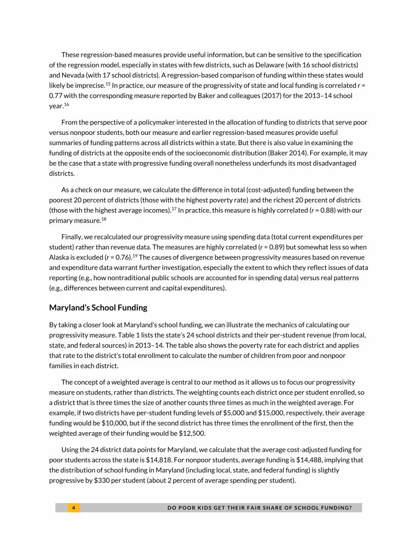
These regression-based measures provide useful information, but can be sensitive to the specification
of the regression model, especially in states with few districts, such as Delaware (with 16 school districts)
and Nevada (with 17 school districts). A regression-based comparison of funding within these states would
likely be imprecise.15 In practice, our measure of the progressivity of state and local funding is correlated r =
0.77 with the corresponding measure reported by Baker and colleagues (2017) for the 2013–14 school
year.16
From the perspective of a policymaker interested in the allocation of funding to districts that serve poor
versus nonpoor students, both our measure and earlier regression-based measures provide useful
summaries of funding patterns across all districts within a state. But there is also value in examining the
funding of districts at the opposite ends of the socioeconomic distribution (Baker 2014). For example, it may
be the case that a state with progressive funding overall nonetheless underfunds its most disadvantaged
districts.
As a check on our measure, we calculate the difference in total (cost-adjusted) funding between the
poorest 20 percent of districts (those with the highest poverty rate) and the richest 20 percent of districts
(those with the highest average incomes).17 In practice, this measure is highly correlated (r = 0.88) with our
primary measure.18
Finally, we recalculated our progressivity measure using spending data (total current expenditures per
student) rather than revenue data. The measures are highly correlated (r = 0.89) but somewhat less so when
Alaska is excluded (r = 0.76).19 The causes of divergence between progressivity measures based on revenue
and expenditure data warrant further investigation, especially the extent to which they reflect issues of data
reporting (e.g., how nontraditional public schools are accounted for in spending data) versus real patterns
(e.g., differences between current and capital expenditures).
Maryland’s School Funding
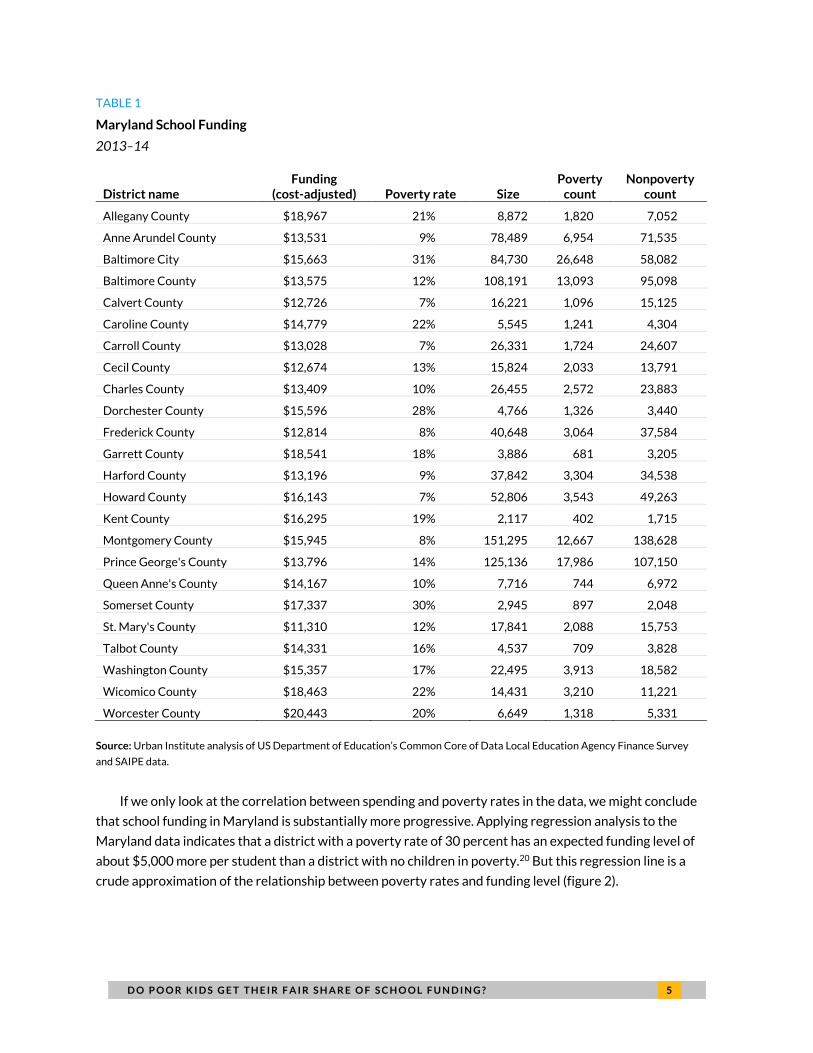
By taking a closer look at Maryland’s school funding, we can illustrate the mechanics of calculating our
progressivity measure. Table 1 lists the state’s 24 school districts and their per-student revenue (from local,
state, and federal sources) in 2013–14. The table also shows the poverty rate for each district and applies
that rate to the district’s total enrollment to calculate the number of children from poor and nonpoor
families in each district.
The concept of a weighted average is central to our method as it allows us to focus our progressivity
measure on students, rather than districts. The weighting counts each district once per student enrolled, so
a district that is three times the size of another counts three times as much in the weighted average. For
example, if two districts have per-student funding levels of $5,000 and $15,000, respectively, their average
funding would be $10,000, but if the second district has three times the enrollment of the first, then the
weighted average of their funding would be $12,500.
Using the 24 district data points for Maryland, we calculate that the average cost-adjusted funding for
poor students across the state is $14,818. For nonpoor students, average funding is $14,488, implying that
the distribution of school funding in Maryland (including local, state, and federal funding) is slightly
progressive by $330 per student (about 2 percent of average spending per student).
D O P O O R K I D S G E T T H E I R F A I R S H A R E O F S C H O O L F U N D I N G ? 5
TABLE 1
Maryland School Funding
2013–14
District name Funding
(cost-adjusted) Poverty rate Size Poverty
count Nonpoverty
count
Allegany County $18,967 21% 8,872 1,820 7,052
Anne Arundel County $13,531 9% 78,489 6,954 71,535
Baltimore City $15,663 31% 84,730 26,648 58,082
Baltimore County $13,575 12% 108,191 13,093 95,098
Calvert County $12,726 7% 16,221 1,096 15,125
Caroline County $14,779 22% 5,545 1,241 4,304
Carroll County $13,028 7% 26,331 1,724 24,607
Cecil County $12,674 13% 15,824 2,033 13,791
Charles County $13,409 10% 26,455 2,572 23,883
Dorchester County $15,596 28% 4,766 1,326 3,440
Frederick County $12,814 8% 40,648 3,064 37,584
Garrett County $18,541 18% 3,886 681 3,205
Harford County $13,196 9% 37,842 3,304 34,538
Howard County $16,143 7% 52,806 3,543 49,263
Kent County $16,295 19% 2,117 402 1,715
Montgomery County $15,945 8% 151,295 12,667 138,628
Prince George's County $13,796 14% 125,136 17,986 107,150
Queen Anne's County $14,167 10% 7,716 744 6,972
Somerset County $17,337 30% 2,945 897 2,048
St. Mary's County $11,310 12% 17,841 2,088 15,753
Talbot County $14,331 16% 4,537 709 3,828
Washington County $15,357 17% 22,495 3,913 18,582
Wicomico County $18,463 22% 14,431 3,210 11,221
Worcester County $20,443 20% 6,649 1,318 5,331
Source: Urban Institute analysis of US Department of Education’s Common Core of Data Local Education Agency Finance Survey
and SAIPE data.
If we only look at the correlation between spending and poverty rates in the data, we might conclude
that school funding in Maryland is substantially more progressive. Applying regression analysis to the
Maryland data indicates that a district with a poverty rate of 30 percent has an expected funding level of
about $5,000 more per student than a district with no children in poverty.20 But this regression line is a
crude approximation of the relationship between poverty rates and funding level (figure 2).

6 D O P O O R K I D S G E T T H E I R F A I R S H A R E O F S C H O O L F U N D I N G ?
FIGURE 2
Maryland School Funding versus Poverty Rate
2013–14
Source: Urban Institute analysis of US Department of Education’s Common Core of Data Local Education Agency Finance Survey
and SAIPE data.
Note: The size of each dot corresponds to the enrollment of poor students.
Measuring the relationship between poverty rates and funding and closely examining districts that
serve large populations of disadvantaged students (e.g., Baltimore) is useful for understanding the broad
trends of school funding within a state. But our measure has the benefit of assessing funding for all poor
students in Maryland, including the 76 percent not in Baltimore and the 63 percent who are enrolled in
districts with poverty rates below 15 percent. Additionally, our measure is based on actual (cost-adjusted)
funding data, rather than a prediction from a regression model that may rely on a relatively small number of
data points (only 24 in the Maryland example).
School Funding Progressivity in 49 States
We calculate our student-weighted progressivity measure using cost-adjusted, district-level revenue data
from every state except Hawaii (which is a single district). First, we estimate the progressivity of both local
and state funding, demonstrating how formula-driven state funding often counteracts regressive local
funding. We then apply our measure to the overall levels of school district funding, showing how federal
funds also target districts with more poor students.
$10,000
$12,000
$14,000
$16,000
$18,000
$20,000
$22,000
5% 10% 15% 20% 25% 30% 35%Poverty rate
Per-student funding (cost-adjusted)
D O P O O R K I D S G E T T H E I R F A I R S H A R E O F S C H O O L F U N D I N G ? 7
Funding levels vary much more across states than they do between poor and nonpoor students within
the same state.
Unsurprisingly, revenues from local sources tend to be lowest in districts with more poor students. Per-
student local revenues are more than $3,000 lower among the districts attended by poor students in
Connecticut, relative to the districts attended by nonpoor students. Because property wealth is unequally
distributed among school districts within a state, school districts vary in the amount of local funding that
they can raise from property taxes.
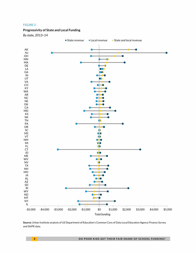
Many states’ education funding from the state government is designed to counteract this imbalance.
Figure 3 orders states based on the progressivity of their combined state and local funding. In nearly every
state, regressive local funding is balanced to varying degrees by progressive state funding.21 The states with
the more regressive local funding are often those that go to the greatest lengths to provide progressive
state funding. These include several states that have faced court orders over their funding systems, such as
New Jersey, Connecticut, Massachusetts, and Ohio (Lafortune, Rothstein, and Schazenbach2016).
However, even with progressive state funding, about half of the states in our study still distribute
relatively more local and state funding to students not in poverty. Federal funding to school districts, such as
Title I funding, is specifically designed to target low-income students, as well as other high-needs students.22
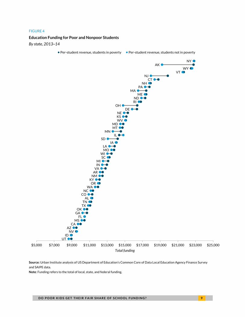
Figure 4 shows that, with the addition of federal dollars, total funding is regressive in only three states:
Illinois (-$431), Wyoming ($-131), and Nevada (-$69).
The addition of federal funding tips the overall balance of states to most being in the progressive
category. But, even with federal dollars, only a handful of states attain a high level of progressivity. Our
progressivity measure exceeds $1,000 per student in only four states (South Dakota, Ohio, New Jersey, and
Alaska).
We also see that funding levels vary much more across states than they do between poor and nonpoor
students within the same state (figure 4). There are compelling reasons to believe that both absolute and
relative expenditures matter. For example, with all else equal, a state with higher teacher salaries should be
expected to have more people interested in teaching (and thus a larger pool from which to hire teachers)
than a lower-spending state. And, within a low-spending state, districts with more money to spend are, all
else equal, better positioned to compete for teaching talent within the state than districts with less funding.
8 D O P O O R K I D S G E T T H E I R F A I R S H A R E O F S C H O O L F U N D I N G ?
FIGURE 3
Progressivity of State and Local Funding
By state, 2013–14
Source: Urban Institute analysis of US Department of Education’s Common Core of Data Local Education Agency Finance Survey
and SAIPE data.
-$5,000 -$4,000 -$3,000 -$2,000 -$1,000 $0 $1,000 $2,000 $3,000 $4,000 $5,000
ILNYMTNDWY
RISDAZALIA
MONHTX
NVWVME
IDCTFLMI
NMVTMSSC
ORPATNWIKS
MDCAOKNENCAR
WAKYCOVAUTIN
GALADE
MAMNOHNJAK
Total funding
State revenue Local revenue State and local revenue
D O P O O R K I D S G E T T H E I R F A I R S H A R E O F S C H O O L F U N D I N G ? 9
FIGURE 4
Education Funding for Poor and Nonpoor Students
By state, 2013–14
Source: Urban Institute analysis of US Department of Education’s Common Core of Data Local Education Agency Finance Survey
and SAIPE data.
Note: Funding refers to the total of local, state, and federal funding.
UTID
NVAZ
CAMS
FLGA
OKTXTN
ALCO
NCWA
ORKY
NMAR
VAINMI
SCWI
MOLA
IASD
ILMN
MTMD
WVKSNE
DEOH
RIND
MEMA
PANH
CTNJ
VTWY
AKNY
$5,000 $7,000 $9,000 $11,000 $13,000 $15,000 $17,000 $19,000 $21,000 $23,000 $25,000
Total funding
Per-student revenue, students in poverty Per-student revenue, students not in poverty
1 0 D O P O O R K I D S G E T T H E I R F A I R S H A R E O F S C H O O L F U N D I N G ?
Education Funding Is as Progressive Today as It Was in
1995
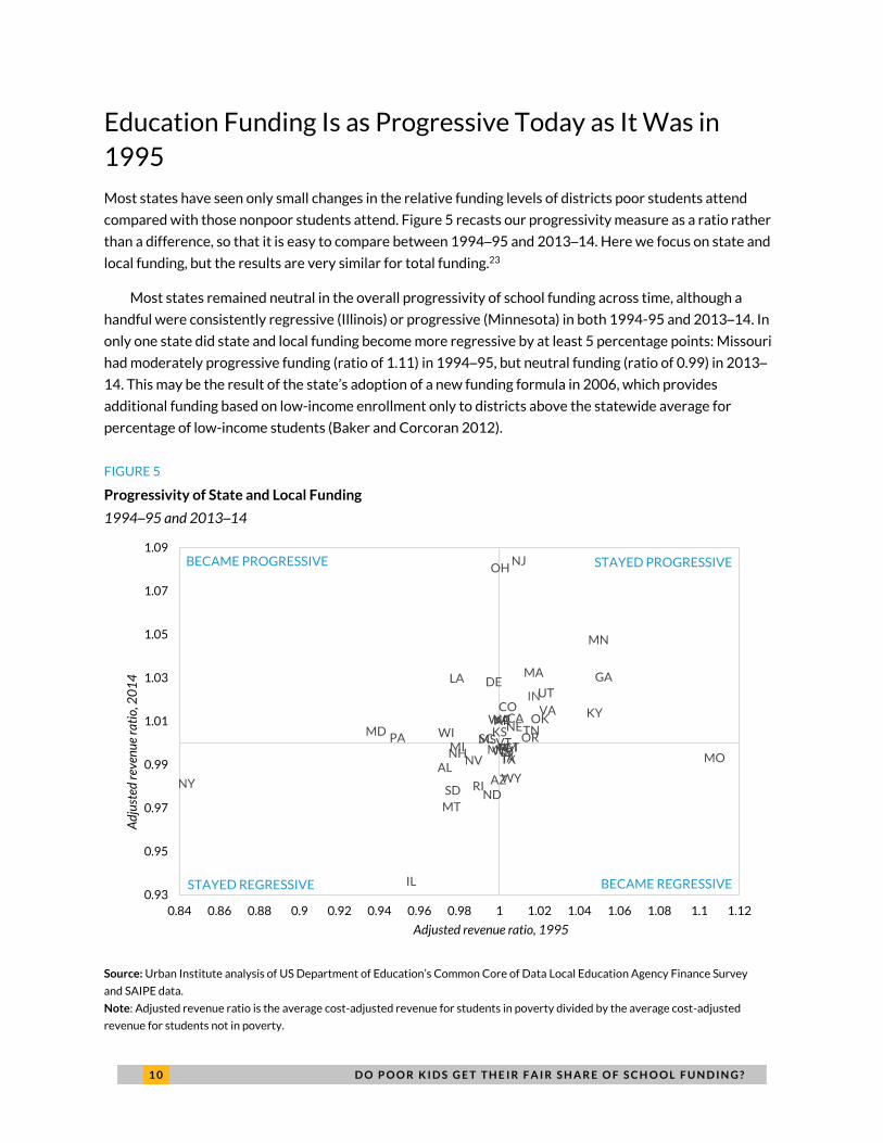
Most states have seen only small changes in the relative funding levels of districts poor students attend
compared with those nonpoor students attend. Figure 5 recasts our progressivity measure as a ratio rather
than a difference, so that it is easy to compare between 1994–95 and 2013–14. Here we focus on state and
local funding, but the results are very similar for total funding.23
Most states remained neutral in the overall progressivity of school funding across time, although a
handful were consistently regressive (Illinois) or progressive (Minnesota) in both 1994-95 and 2013–14. In
only one state did state and local funding become more regressive by at least 5 percentage points: Missouri
had moderately progressive funding (ratio of 1.11) in 1994–95, but neutral funding (ratio of 0.99) in 2013–
14. This may be the result of the state’s adoption of a new funding formula in 2006, which provides
additional funding based on low-income enrollment only to districts above the statewide average for
percentage of low-income students (Baker and Corcoran 2012).
FIGURE 5
Progressivity of State and Local Funding
1994–95 and 2013–14
Source: Urban Institute analysis of US Department of Education’s Common Core of Data Local Education Agency Finance Survey
and SAIPE data.
Note: Adjusted revenue ratio is the average cost-adjusted revenue for students in poverty divided by the average cost-adjusted
revenue for students not in poverty.
AL
AR
AZ
CACO
CT
DE
FL
GA
IAID
IL
IN
KS
KY
LA MA
MD
MEMI
MN
MO
MS
MT
NC
ND
NE
NH
NJ
NMNV
NY
OH
OK
ORPA
RI
SC
SD
TN
TX
UT
VA
VT
WAWI
WV
WY
0.93
0.95
0.97
0.99
1.01
1.03
1.05
1.07
1.09
0.84 0.86 0.88 0.9 0.92 0.94 0.96 0.98 1 1.02 1.04 1.06 1.08 1.1 1.12
Ad
just
ed r
even
ue
rati
o, 2
01
4
Adjusted revenue ratio, 1995
STAYED PROGRESSIVEBECAME PROGRESSIVE
STAYED REGRESSIVE BECAME REGRESSIVE
D O P O O R K I D S G E T T H E I R F A I R S H A R E O F S C H O O L F U N D I N G ? 1 1
Six states experienced an increase in the progressivity of state and local funding of at least 5 percentage
points. Four of those states went from regressive to approximately neutral (Louisiana, Pennsylvania,
Maryland, and New York), and two went from neutral to progressive (New Jersey and Ohio). Maryland, New
York, New Jersey, and Ohio all made court-ordered changes to their funding systems during this period
(Lafortune, Rothstein, and Schazenbach 2016).
Economic Segregation and Funding Progressivity
The segregation of students by race and income is well documented. What is less well understood is how
states with more segregated school districts can more readily target poor students because those students
are more concentrated within certain districts. In states where school districts vary less in terms of
demographics, such as those with large, countywide districts, it is harder to direct funding to disadvantaged
students.
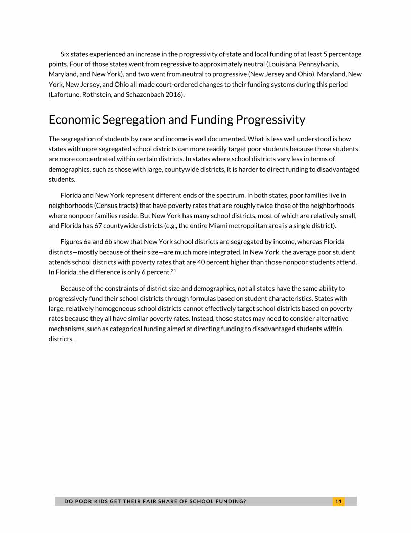
Florida and New York represent different ends of the spectrum. In both states, poor families live in
neighborhoods (Census tracts) that have poverty rates that are roughly twice those of the neighborhoods
where nonpoor families reside. But New York has many school districts, most of which are relatively small,
and Florida has 67 countywide districts (e.g., the entire Miami metropolitan area is a single district).
Figures 6a and 6b show that New York school districts are segregated by income, whereas Florida
districts—mostly because of their size—are much more integrated. In New York, the average poor student
attends school districts with poverty rates that are 40 percent higher than those nonpoor students attend.
In Florida, the difference is only 6 percent.24
Because of the constraints of district size and demographics, not all states have the same ability to
progressively fund their school districts through formulas based on student characteristics. States with
large, relatively homogeneous school districts cannot effectively target school districts based on poverty
rates because they all have similar poverty rates. Instead, those states may need to consider alternative
mechanisms, such as categorical funding aimed at directing funding to disadvantaged students within
districts.
1 2 D O P O O R K I D S G E T T H E I R F A I R S H A R E O F S C H O O L F U N D I N G ?
FIGURE 6A
Economic Segregation of Census Tracts versus School Districts
Florida
Poverty rate among families with children ages 5–17
FIGURE 6B
Economic Segregation of Census Tracts versus School Districts
New York
Poverty rate among families with children ages 5–17
Source: Urban Institute analysis of 2015 five-year estimates from the American Community Survey.
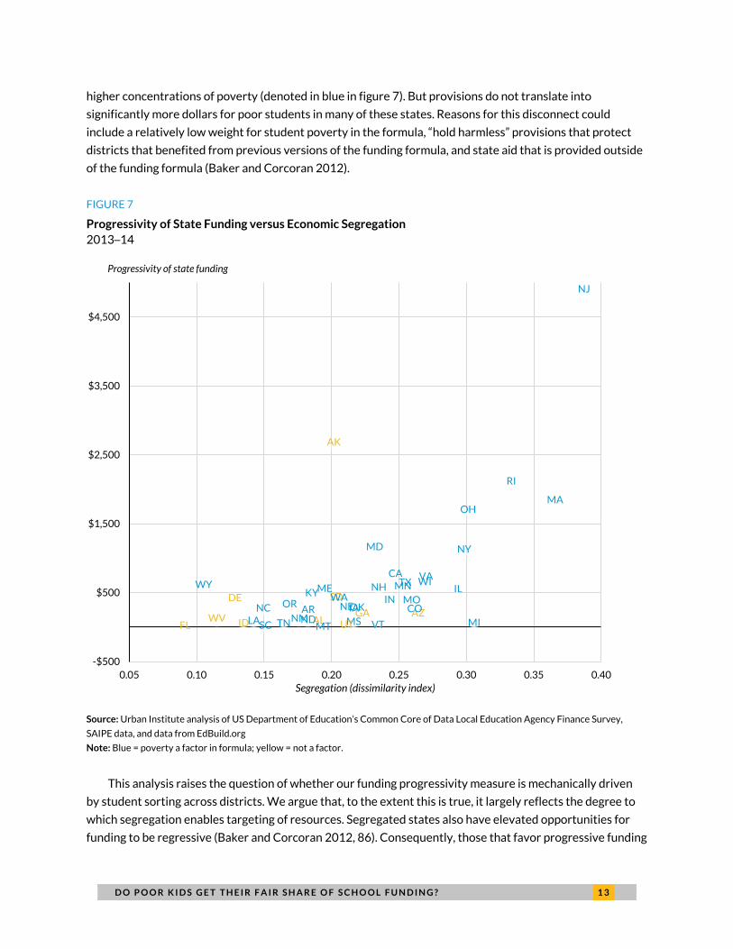
At the same time, there are many states that could have progressive formula-based funding but do not.
Figure 7 shows that funding provided by the state is not particularly progressive in many states where it
could be (given segregation levels), including Vermont, Mississippi, Colorado, and Michigan.
Policymakers in most of these states have at least some interest in providing progressive funding, as
indicated by the funding formula providing additional funds for districts with more children in poverty or
D O P O O R K I D S G E T T H E I R F A I R S H A R E O F S C H O O L F U N D I N G ? 1 3
higher concentrations of poverty (denoted in blue in figure 7). But provisions do not translate into
significantly more dollars for poor students in many of these states. Reasons for this disconnect could
include a relatively low weight for student poverty in the formula, “hold harmless” provisions that protect
districts that benefited from previous versions of the funding formula, and state aid that is provided outside
of the funding formula (Baker and Corcoran 2012).
FIGURE 7
Progressivity of State Funding versus Economic Segregation
2013–14
Source: Urban Institute analysis of US Department of Education’s Common Core of Data Local Education Agency Finance Survey,
SAIPE data, and data from EdBuild.org
Note: Blue = poverty a factor in formula; yellow = not a factor.
This analysis raises the question of whether our funding progressivity measure is mechanically driven
by student sorting across districts. We argue that, to the extent this is true, it largely reflects the degree to
which segregation enables targeting of resources. Segregated states also have elevated opportunities for
funding to be regressive (Baker and Corcoran 2012, 86). Consequently, those that favor progressive funding
AK
ALAR AZ
CA
CODE
FLGAIA
ID
ILIN
KY
LA
MA
MD
ME
MI
MN
MO
MSMT
NCND
NE
NH
NJ
NM
NY
OH
OKOR
RI
SC
SD
TN
TX
UT
VA
VT
WA
WI
WV
WY
-$500
$500
$1,500
$2,500
$3,500
$4,500
0.05 0.10 0.15 0.20 0.25 0.30 0.35 0.40
Segregation (dissimilarity index)
Progressivity of state funding
1 4 D O P O O R K I D S G E T T H E I R F A I R S H A R E O F S C H O O L F U N D I N G ?
systems should be encouraged by the fact that funding is not regressively distributed across districts in
states with the highest levels of economic segregation across districts.
Conclusion
We find that poor students in most states attend school districts that are about as well funded as the
districts nonpoor students attend in their state. This is good news for those concerned about regressive
funding, but troubling news for those who advocate for additional funding for schools serving low-income
students. With a few notable exceptions, such as New Jersey and Ohio, districts serving poor students do
not receive significantly more resources than districts that serve nonpoor students.
Many states have adopted funding systems aimed at providing more resources to schools serving
disadvantaged students. Our analysis indicates that funding progressivity has not changed much since 1995,
perhaps because local funding has responded in ways that tend to preserve the relative funding of more
versus less economically advantaged districts. The ways in which state and local funding interact is an
important subject for future research.
Regardless of their overall effect on progressivity in the medium to long run, the funding reforms of the
1990s and 2000s appear to have benefited disadvantaged students (Jackson, Johnson, and Persico 2016;
Lafortune , Rothstein, and Schazenbach 2016). But policy design clearly matters, as shown by the continued
general lack of progressivity in many states documented here and by previous research on state funding
policies (e.g., Baker and Corcoran 2012). For example, a 1994 Michigan funding reform disproportionately
benefited more advantaged students, likely because districts directed new dollars to schools serving less-
poor student populations (Hyman, forthcoming).
Debates over school funding levels are probably as old as the education system itself. Opponents of
spending more on schools can point to examples of funding that is either wasted (e.g., additional pay to
teachers with master’s degrees [Chingos and Peterson 2010]) or of questionable cost-effectiveness (e.g.,
across-the-board reductions in class size [Chingos 2013]). But there are also examples of interventions that
cost money and are effective (e.g., intensive tutoring of low-income students [Cook et al. 2015]), as well as
evidence that disadvantaged students have benefited from unrestricted funding increases (Jackson,
Johnson, and Persico 2016).
The challenge states face is to find the right set of funding policies to accomplish their objectives given
their historical, institutional, and political constraints. For some states, that may mean aggressive
redistribution across districts that are highly segregated by income through funding formulas that gives
districts flexibility on how funds are spent. Other states may prefer—or need—to use a combination of
formula and categorical funding to ensure that funds reach students who need them the most.

D O P O O R K I D S G E T T H E I R F A I R S H A R E O F S C H O O L F U N D I N G ? 1 5
Appendix. Data and Alternative Measures
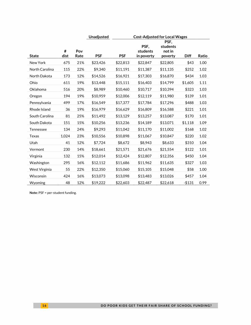
TABLE A.1
School Funding Data
By state, 2013-14
Unadjusted Cost-Adjusted for Local Wages
State #
dist Pov Rate PSF PSF
PSF, students
in poverty
PSF, students
not in poverty Diff Ratio
Alabama 135 25% $9,889 $11,221 $11,287 $11,199 $88 1.01
Alaska 53 15% $19,572 $19,730 $22,778 $19,211 $3,568 1.19
Arizona 206 23% $8,736 $9,279 $9,511 $9,208 $304 1.03
Arkansas 238 24% $10,605 $12,260 $12,486 $12,188 $298 1.02
California 921 22% $10,813 $9,757 $9,990 $9,693 $296 1.03
Colorado 178 14% $10,489 $10,962 $11,305 $10,904 $401 1.04
Connecticut 166 14% $20,041 $18,425 $18,793 $18,366 $427 1.02
Delaware 16 17% $15,887 $15,916 $16,371 $15,820 $551 1.03
Florida 67 22% $9,630 $10,427 $10,448 $10,420 $28 1.00
Georgia 180 25% $10,440 $10,333 $10,709 $10,210 $499 1.05
Idaho 114 17% $7,403 $8,906 $8,956 $8,896 $60 1.01
Illinois 852 18% $14,555 $14,735 $14,359 $14,820 -$461 0.97
Indiana 289 18% $12,179 $12,538 $12,964 $12,443 $521 1.04
Iowa 344 14% $12,605 $13,998 $14,047 $13,990 $57 1.00
Kansas 285 16% $11,705 $14,879 $15,172 $14,822 $350 1.02
Kentucky 173 24% $10,676 $11,853 $12,133 $11,766 $367 1.03
Louisiana 68 25% $12,271 $13,399 $13,842 $13,250 $592 1.04
Maine 181 16% $14,772 $17,301 $17,418 $17,278 $140 1.01
Maryland 24 13% $16,150 $14,531 $14,818 $14,488 $331 1.02
Massachusetts 295 14% $17,852 $16,628 $17,423 $16,501 $921 1.06
Michigan 541 18% $11,547 $12,630 $13,105 $12,525 $581 1.05
Minnesota 330 13% $13,271 $13,752 $14,547 $13,635 $912 1.07
Mississippi 148 29% $9,097 $10,202 $10,419 $10,115 $305 1.03
Missouri 518 18% $11,027 $13,538 $13,781 $13,483 $298 1.02
Montana 407 18% $11,843 $14,495 $14,729 $14,445 $285 1.02
Nebraska 249 14% $12,589 $14,975 $15,338 $14,915 $423 1.03
Nevada 17 20% $9,646 $9,544 $9,489 $9,558 -$69 0.99
New Hampshire 162 11% $16,456 $17,790 $17,917 $17,775 $142 1.01
New Jersey 543 14% $20,677 $18,222 $19,861 $17,947 $1,914 1.11
New Mexico 89 26% $11,026 $12,224 $12,466 $12,140 $326 1.03
1 6 D O P O O R K I D S G E T T H E I R F A I R S H A R E O F S C H O O L F U N D I N G ?
Unadjusted Cost-Adjusted for Local Wages
State #
dist Pov Rate PSF PSF
PSF, students
in poverty
PSF, students
not in poverty Diff Ratio
New York 675 21% $23,426 $22,813 $22,847 $22,805 $43 1.00
North Carolina 115 22% $9,340 $11,191 $11,387 $11,135 $252 1.02
North Dakota 173 12% $14,526 $16,921 $17,303 $16,870 $434 1.03
Ohio 611 19% $13,448 $15,111 $16,403 $14,799 $1,605 1.11
Oklahoma 516 20% $8,989 $10,460 $10,717 $10,394 $323 1.03
Oregon 194 19% $10,959 $12,006 $12,119 $11,980 $139 1.01
Pennsylvania 499 17% $16,549 $17,377 $17,784 $17,296 $488 1.03
Rhode Island 36 19% $16,979 $16,629 $16,809 $16,588 $221 1.01
South Carolina 81 25% $11,492 $13,129 $13,257 $13,087 $170 1.01
South Dakota 151 15% $10,256 $13,236 $14,189 $13,071 $1,118 1.09
Tennessee 134 24% $9,293 $11,042 $11,170 $11,002 $168 1.02
Texas 1,024 23% $10,556 $10,898 $11,067 $10,847 $220 1.02
Utah 41 12% $7,724 $8,672 $8,943 $8,633 $310 1.04
Vermont 230 14% $18,661 $21,571 $21,676 $21,554 $122 1.01
Virginia 132 15% $12,014 $12,424 $12,807 $12,356 $450 1.04
Washington 295 16% $12,112 $11,686 $11,962 $11,635 $327 1.03
West Virginia 55 22% $12,350 $15,060 $15,105 $15,048 $58 1.00
Wisconsin 424 16% $13,073 $13,098 $13,483 $13,026 $457 1.04
Wyoming 48 12% $19,222 $22,603 $22,487 $22,618 -$131 0.99
Note: PSF = per-student funding.
D O P O O R K I D S G E T T H E I R F A I R S H A R E O F S C H O O L F U N D I N G ? 1 7
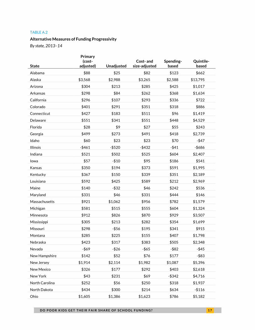
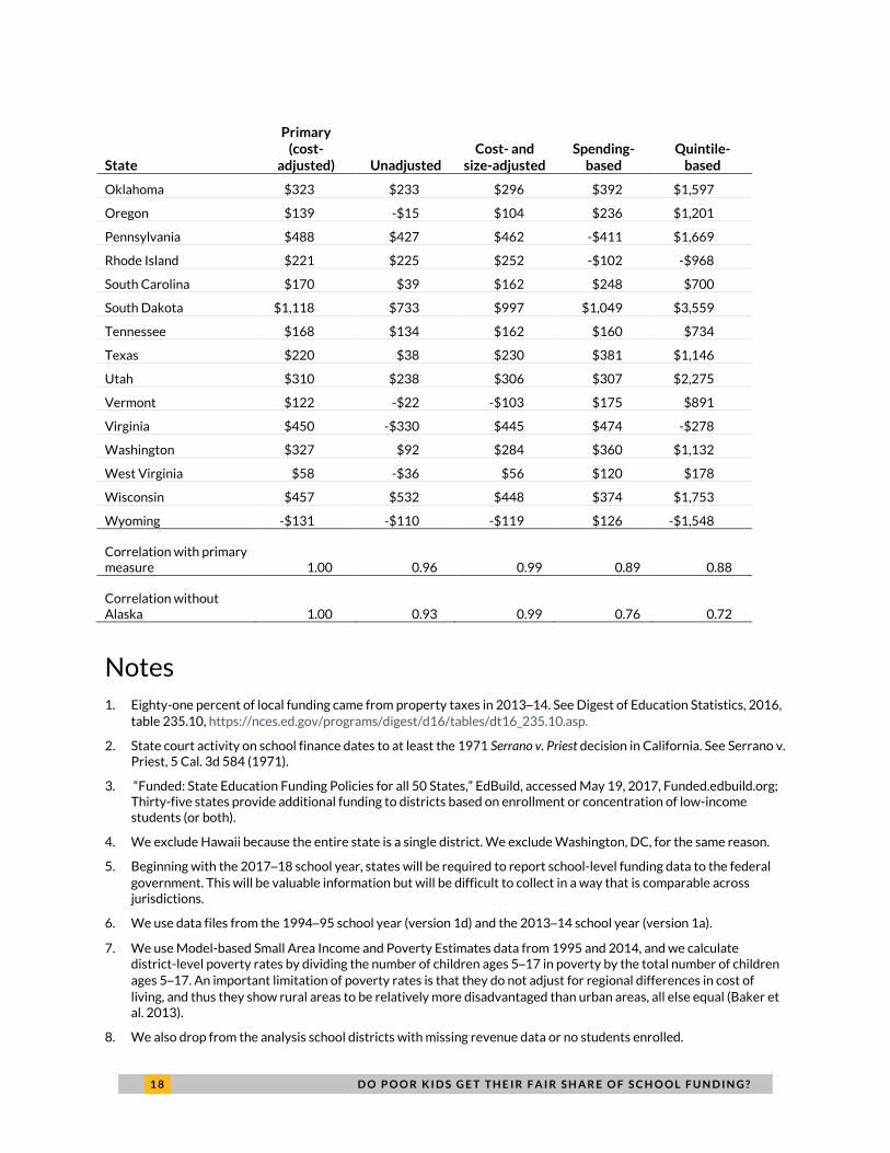
TABLE A.2
Alternative Measures of Funding Progressivity
By state, 2013–14
State
Primary (cost-
adjusted) Unadjusted Cost- and
size-adjusted Spending-
based Quintile-
based
Alabama $88 $25 $82 $123 $662
Alaska $3,568 $2,988 $3,265 $2,588 $13,795
Arizona $304 $213 $285 $425 $1,017
Arkansas $298 $84 $262 $368 $1,634
California $296 $107 $293 $336 $722
Colorado $401 $291 $351 $318 $886
Connecticut $427 $183 $511 $96 $1,419
Delaware $551 $341 $551 $448 $4,529
Florida $28 $9 $27 $55 $243
Georgia $499 $273 $491 $418 $2,739
Idaho $60 $23 $23 $70 -$47
Illinois -$461 -$520 -$432 -$41 -$686
Indiana $521 $502 $525 $604 $2,407
Iowa $57 -$10 $95 $186 $541
Kansas $350 $194 $373 $591 $1,995
Kentucky $367 $150 $339 $351 $2,189
Louisiana $592 $425 $589 $212 $2,969
Maine $140 -$32 $46 $242 $536
Maryland $331 $46 $331 $444 $146
Massachusetts $921 $1,062 $956 $782 $1,579
Michigan $581 $515 $555 $604 $1,324
Minnesota $912 $826 $870 $929 $3,507
Mississippi $305 $213 $282 $354 $1,699
Missouri $298 -$56 $195 $341 $915
Montana $285 $225 $155 $407 $1,798
Nebraska $423 $317 $383 $505 $2,348
Nevada -$69 -$26 -$65 -$82 -$45
New Hampshire $142 $52 $76 $177 -$83
New Jersey $1,914 $2,114 $1,982 $1,087 $5,396
New Mexico $326 $177 $292 $403 $2,618
New York $43 $231 $69 -$342 $4,716
North Carolina $252 $56 $250 $318 $1,937
North Dakota $434 $300 $214 $634 -$116
Ohio $1,605 $1,386 $1,623 $786 $5,182
1 8 D O P O O R K I D S G E T T H E I R F A I R S H A R E O F S C H O O L F U N D I N G ?
State
Primary (cost-
adjusted) Unadjusted Cost- and
size-adjusted Spending-
based Quintile-
based
Oklahoma $323 $233 $296 $392 $1,597
Oregon $139 -$15 $104 $236 $1,201
Pennsylvania $488 $427 $462 -$411 $1,669
Rhode Island $221 $225 $252 -$102 -$968
South Carolina $170 $39 $162 $248 $700
South Dakota $1,118 $733 $997 $1,049 $3,559
Tennessee $168 $134 $162 $160 $734
Texas $220 $38 $230 $381 $1,146
Utah $310 $238 $306 $307 $2,275
Vermont $122 -$22 -$103 $175 $891
Virginia $450 -$330 $445 $474 -$278
Washington $327 $92 $284 $360 $1,132
West Virginia $58 -$36 $56 $120 $178
Wisconsin $457 $532 $448 $374 $1,753
Wyoming -$131 -$110 -$119 $126 -$1,548
Correlation with primary measure 1.00 0.96 0.99 0.89 0.88
Correlation without Alaska 1.00 0.93 0.99 0.76 0.72
Notes
1. Eighty-one percent of local funding came from property taxes in 2013–14. See Digest of Education Statistics, 2016,
table 235.10, https://nces.ed.gov/programs/digest/d16/tables/dt16_235.10.asp.
2. State court activity on school finance dates to at least the 1971 Serrano v. Priest decision in California. See Serrano v. Priest, 5 Cal. 3d 584 (1971).
3. “Funded: State Education Funding Policies for all 50 States,” EdBuild, accessed May 19, 2017, Funded.edbuild.org; Thirty-five states provide additional funding to districts based on enrollment or concentration of low-income students (or both).
4. We exclude Hawaii because the entire state is a single district. We exclude Washington, DC, for the same reason.
5. Beginning with the 2017–18 school year, states will be required to report school-level funding data to the federal
government. This will be valuable information but will be difficult to collect in a way that is comparable across jurisdictions.
6. We use data files from the 1994–95 school year (version 1d) and the 2013–14 school year (version 1a).
7. We use Model-based Small Area Income and Poverty Estimates data from 1995 and 2014, and we calculate district-level poverty rates by dividing the number of children ages 5–17 in poverty by the total number of children
ages 5–17. An important limitation of poverty rates is that they do not adjust for regional differences in cost of
living, and thus they show rural areas to be relatively more disadvantaged than urban areas, all else equal (Baker et al. 2013).
8. We also drop from the analysis school districts with missing revenue data or no students enrolled.

D O P O O R K I D S G E T T H E I R F A I R S H A R E O F S C H O O L F U N D I N G ? 1 9
9. National Center for Education Statistics Comparable Wage Index; see also Taylor et al. 2007. Specifically, we calculate adjusted per-student funding as actual per-student funding in 2013–14 divided by the American
Community Survey–based comparable wage index for 2012–14.
10. This adjustment implicitly uses the wage index as a proxy for all costs districts face, including labor and nonlabor costs. It therefore does not consider other variation in district costs, such as those that result from differences in district size and density (e.g., we might expect a larger district to require lower per-student funding because of efficiency gains, all else equal, and a sparser district to require more funding, because of increased transportation costs). We experimented with regression-based adjustment models along the lines of those used by Baker (2016) and Baker et al. (2017), but found the resulting state-level progressivity estimates to be sensitive to the model specification. We also decided against using a regression-based model because it reflects differences in district-specific cost functions (which we want to account for) and differences in policy decisions that are correlated with cost drivers (which we do not want to account for). For example, a regression-based model that includes district size reflects both possible economies to scale that larger districts enjoy as well as the fact that larger districts (which tend to be located in cities) may spend more or less, on average, than other districts for other reasons (such as political ones).
11. The mean progressivity measure is similar and the correlation between the measures based on raw and cost-adjusted data is 0.96.
12. The most notable exception is Virginia, where the raw data indicate that funding is regressive by $330 per student and the cost-adjusted measure shows that funding is progressive by $450 per student. Unadjusted metrics for each state are reported in appendix table A.2.
13. As a robustness check, we adjust downward the funding of relatively small districts (those with fewer than 1,500 students, or about 58 percent of districts). Specifically, we apply the following adjustment to log(funding) for these districts: exp(log(adj_revpp1)−((10.553*size^−0.014)−9.526)). This adjustment is based on the observed relationship between log(funding) and district size nationwide. We find that the cost- and size-adjusted estimates are highly correlated (r=0.99) with the cost-adjusted estimates (see appendix table A.2).
14. Lafortune, Rothstein, and Schanzenbach (2016) also estimate the within-state relationship between district-level spending and average family income, controlling for enrollment.
15. Earlier research has estimated national models with state-specific poverty-funding gradients (see, for example, Baker 2016), which estimate more precise funding-covariate relationships but assume that those relationships are constant across states and are still based on a small number of observations for estimating the poverty-funding gradient in some states.
16. Baker et al. (2017) do not report a value for Alaska, so the correlation excludes this data point. Weighted by the number of districts in each state, the correlation is r = 0.92, suggesting that the two measures diverge the most among states with fewer districts.
17. We identify quintiles weighted by student enrollment. We drop the handful of districts with high poverty rates and high average incomes. Income is measured as median income of families with children younger than 18 in the 2010–14 American Community Survey (five-year estimates).
18. See appendix table A.2. The most notable difference between the two measures is New York, which is one of the least progressive states based on our preferred measure, but it is one of the most progressive states when looking at the richest versus poorest districts. However, New York again appears to be regressive if we look at raw spending instead of cost-adjusted spending (even though the raw and cost-adjusted versions of our alternative measure are correlated r = 0.88). We caution readers against reading too much into any of the results for New York given their unusually high sensitivity to methodology.
19. The corresponding revenue (from all sources) and spending progressivity measures in the “School Funding Fairness Data System” data have the same level of correlation (r = 0.76); see Bruce D. Baker, Ajay Srikanth, and Mark Weber, “Rutgers Graduate School of Education/Education Law Center: School Funding Fairness Data System,” 2016, http://www.schoolfundingfairness.org/data-download.
20. Weighting the regression by total enrollment in each district reduces the change in funding predicted ($5,234 to $2,168) by a 30 percentage point change.
21. State and local funding can interact, in that districts that receive more state funding may reduce the amount of local funding that they provide. In other words, progressive systems of state funding can (at least in theory) cause the distribution of local funding to be more regressive.

2 0 D O P O O R K I D S G E T T H E I R F A I R S H A R E O F S C H O O L F U N D I N G ?
22. Our progressivity measures are based on cost-adjusted data, but federal and state funding formulas are generally not cost adjusted. However, as noted earlier, the cost adjustment does not have a large effect on our progressivity measures. For example, our raw and cost-adjusted estimates of the progressivity of federal funding are highly correlated (r = 0.98).
23. For all combinations, see Alex Tilsley, “School Funding: Do Poor Kids Get Their Fair Share?” Urban Institute, June 2017, http://apps.urban.org/features/school-funding-do-poor-kids-get-fair-share.
24. We also calculate dissimilarity indices, which are 0.40 for Florida Census tracts, 0.46 for New York Census tracts, 0.11 for Florida school districts, and 0.30 for New York districts.
References
Baker, Bruce D. 2014. America’s Most Financially Disadvantaged School Districts and How They Got that Way: How State and Local Governance Causes School Funding Disparities. Washington, DC: Center for American Progress.
Baker, Bruce D. 2016. “School Finance and the Distribution of Equal Educational Opportunity in the Postrecession US.” Education Inequality: Opportunity and Mobility 72 (4) 629–55.
Baker, Bruce D., and Sean P. Corcoran. 2012. The Stealth of Inequities of School Funding: How State and Local School Finance Systems Perpetuate Inequitable Student Spending. Washington, DC: Center for American Progress.
Baker, Bruce D., Danielle Farrie, Monete Johnson, Theresa Luhm, and David G. Sciarra. 2017. “Is School Funding Fair? A National Report Card.” New Brunswick, New Jersey: Education Law Center, Rutgers Graduate School of Education.
Baker, Bruce D., Lori Taylor, Jesse Levin, Jay Chambers, and Charles Blankenship. 2013. “Adjusted Poverty Measures and the Distribution of Title I Aid: Does Title I Really Make the Rich States Richer?” Education Finance and Policy 8 (3): 394–417.
Chingos, Matthew M. 2013. “Class Size and Student Outcomes: Research and Policy Implications.” Journal of Policy Analysis and Management 32 (2): 411–38.
Chingos, Matthew M., and Paul E. Peterson. 2010. “It’s Easier to Pick a Good Teacher than to Train One: Familiar and New Results on the Correlates of Teacher Effectiveness.” Economics of Education Review 30 (3): 449–65.
Cook, Philip J., Kenneth Dodge, George Farkas, Roland G. Fryer Jr., Jonathan Guryan, Jens Ludwig, Susan Mayer, Harold Pollack, and Laurence Steinberg. 2015. “Not Too Late: Improving Academic Outcomes for Disadvantaged Youth.” Working Paper Series WP-15-01. Evanston, IL: Institute for Policy Research, Northwestern University.
Hyman, Joshua. Forthcoming. “Does Money Matter in the Long Run? Effects of School Spending on Educational Attainment.” American Economic Journal: Economic Policy.
Jackson, C. Kirabo, Rucker C. Johnson, and Claudia Persico. 2016. “The Effects of School Spending and Economic Outcomes: Evidence from School Finance Reforms.” Quarterly Journal of Economics 131 (1): 157–218.
Lafortune, Julien, Jesse Rothstein, and Diane Whitmore Schazenbach. 2016. “School Finance Reform and the Distribution of Student Achievement.” Working paper. University of California, Berkeley.
Taylor, Lori L., Mark C. Glander, William J. Fowler Jr., Frank Johnson. 2007. Documentation for the NCES Comparable Wage Index Data Files, 2005. Washington, DC: US Department of Education.
About the Authors
Matthew M. Chingos is director of the Urban Institute’s Education Policy Program, which
undertakes policy-relevant research on issues from prekindergarten through
postsecondary education. Current research projects examine universal prekindergarten
programs, school choice, student transportation, school funding, college affordability,
student loan debt, and personalized learning.
D O P O O R K I D S G E T T H E I R F A I R S H A R E O F S C H O O L F U N D I N G ? 2 1
Kristin Blagg is a research associate in the Education Policy Program at the Urban Institute.
Her research focuses on both K–12 and postsecondary education. Blagg has conducted
studies on student transportation and school choice, student loans, and the role of
information in higher education.
Acknowledgments
This brief was funded by Laura and John Arnold Foundation. We are grateful to them and to all our funders,
who make it possible for Urban to advance its mission.
The views expressed are those of the authors and should not be attributed to the Urban Institute, its
trustees, or its funders. Funders do not determine research findings or the insights and recommendations of
Urban experts. Further information on the Urban Institute’s funding principles is available at
www.urban.org/support.
We thank Bruce Baker and Nora Gordon for helpful feedback on earlier drafts of this report.
ABOUT THE URBAN INST IT UTE The nonprofit Urban Institute is dedicated to elevating the debate on social and economic policy. For nearly five decades, Urban scholars have conducted research and offered evidence-based solutions that improve lives and strengthen communities across a rapidly urbanizing world. Their objective research helps expand opportunities for all, reduce hardship among the most vulnerable, and strengthen the effectiveness of the public sector.
Copyright © May 2017. Urban Institute. Permission is granted for reproduction of this file, with attribution to the Urban Institute.
2100 M Street NW Washington, DC 20037
www.urban.org