do not print pantone 032 red guidelines. for...

Modulation and Coding Techniquesin Wireless Communications

Modulation and Coding Techniquesin Wireless Communications M

odulation and Coding Techniquesin W

ireless Comm

unications

Editors

Evgenii KroukSergei Semenov

Editors

KroukSemenov

EditorsEvgenii Krouk, Dean of the Information Systems and Data Protection Faculty, St Petersburg State University of Aerospace Instrumentation, Russia

Sergei Semenov, Specialist, Nokia Corporation, Finland

The high level of technical detail included in standards specifications can make it difficult to find the correlation between the standards specifications and the theoretical results. Thisbook aims to cover both of these elements to give accessible information and support toreaders. It explains the current and future trends on communication theory and shows howthese developments are implemented in contemporary wireless communication standards.

Examining modulation, coding and multiple access techniques, the book is divided into two major sections to cover these functions. The two-stage approach first treats the basics of modulation and coding theory before highlighting how these concepts are defined and implemented in modern wireless communication systems. Part 1 is devoted to thepresentation of main L1 procedures and methods including modulation, coding, channelequalization and multiple access techniques. In Part 2, the uses of these procedures andmethods in the wide range of wireless communication standards including WLAN, WiMax, WCDMA, HSPA, LTE and cdma2000 are considered.

� An essential study of the implementation of modulation and coding techniques in modern standards of wirelesscommunication

� Bridges the gap between the modulation coding theory and the wireless communications standards material

� Divided into two parts to systematically tackle the topic – the first part develops techniques which are then applied and tailored to real world systems in the second part

� Covers special aspects of coding theory and how these can be effectively applied to improve the performance of wireless communications systems

DO NOT PRINT PANTONE 032 RED GUIDELINES. FOR PROOFING ONLY.

P1: TIX/SPH P2: TIX

fm JWST040-Semenov November 11, 2010 15:41 Printer Name: Yet to Come

P1: TIX/SPH P2: TIX


MODULATION ANDCODING TECHNIQUESIN WIRELESSCOMMUNICATIONS

P1: TIX/SPH P2: TIX


P1: TIX/SPH P2: TIX


MODULATION ANDCODING TECHNIQUESIN WIRELESSCOMMUNICATIONS

Edited by

Evgenii KroukDean of the Information Systems and Data Protection Faculty, St Petersburg StateUniversity of Aerospace Instrumentation, Russia

Sergei SemenovSpecialist, Nokia Corporation, Finland

A John Wiley and Sons, Ltd., Publication

P1: TIX/SPH P2: TIX


This edition first published 2011C© 2011 John Wiley & Sons Ltd.

Registered OfficeJohn Wiley & Sons Ltd, The Atrium, Southern Gate, Chichester, West Sussex, PO19 8SQ, United Kingdom

For details of our global editorial offices, for customer services and for information about how to apply forpermission to reuse the copyright material in this book please see our website at www.wiley.com.

The right of the author to be identified as the author of this work has been asserted in accordance with theCopyright, Designs and Patents Act 1988.

All rights reserved. No part of this publication may be reproduced, stored in a retrieval system, or transmitted, inany form or by any means, electronic, mechanical, photocopying, recording or otherwise, except as permitted by theUK Copyright, Designs and Patents Act 1988, without the prior permission of the publisher.

Wiley also publishes its books in a variety of electronic formats. Some content that appears in print may not beavailable in electronic books.

Designations used by companies to distinguish their products are often claimed as trademarks. All brand names andproduct names used in this book are trade names, service marks, trademarks or registered trademarks of theirrespective owners. The publisher is not associated with any product or vendor mentioned in this book. Thispublication is designed to provide accurate and authoritative information in regard to the subject matter covered. Itis sold on the understanding that the publisher is not engaged in rendering professional services. If professionaladvice or other expert assistance is required, the services of a competent professional should be sought.

Library of Congress Cataloging-in-Publication Data

Modulation and coding techniques in wireless communications / edited by Evgenii Krouk, Sergei Semenov.p. cm.

Includes bibliographical references and index.ISBN 978-0-470-74505-2 (cloth)

1. Coding theory. 2. Modulation (Electronics). 3. Wireless communication systems. I. Krouk, E.II. Semenov, S.

TK5102.92.M63 2011621.384–dc22

2010033601

A catalogue record for this book is available from the British Library.

Print ISBN: 9780470745052 [HB]ePDF ISBN:9780470976760oBook ISBN: 9780470976777ePub ISBN: 9780470976715

Typeset in 9/11pt Times by Aptara Inc., New Delhi, India.

http://www.wiley.com

P1: TIX/SPH P2: TIX


Contents

About the Editors xi

List of Contributors xiii

Acknowledgements xv

Introduction xvii

1 Channel Models and Reliable Communication 1Evgenii Krouk, Andrei Ovchinnikov, and Jussi Poikonen

1.1 Principles of Reliable Communication 11.2 AWGN 2

1.2.1 Baseband Representation of AWGN 21.2.2 From Sample SNR to Eb/N0 5

1.3 Fading Processes in Wireless Communication Channels 61.3.1 Large-Scale Fading (Path Loss) 71.3.2 Medium-Scale Fading (Shadowing) 101.3.3 Small-Scale Fading (Multipath Propagation) 11

1.4 Modelling Frequency-Nonselective Fading 141.4.1 Rayleigh and Rice Distributions 141.4.2 Maximum Doppler Frequency Shift 151.4.3 Wide-Sense Stationary Stochastic Processes 151.4.4 Rayleigh and Rice Models for Frequency-Nonselective Fading 151.4.5 SNR in Rayleigh Fading Channels 17

1.5 WSSUS Models for Frequency-Selective Fading 181.5.1 Basic Principles 181.5.2 Definitions 19

References 19

2 Modulation 21Sergei Semenov

2.1 Basic Principles of Bandpass Modulation 212.1.1 The Complex Representation of a Bandpass Signal 222.1.2 Representation of Signal with Basis Functions 272.1.3 Pulse Shaping 312.1.4 Matched Filter 35

2.2 PSK 382.2.1 BPSK 382.2.2 QPSK 43

P1: TIX/SPH P2: TIX


vi Contents

2.2.3 M-PSK 472.2.4 DPSK 482.2.5 OQPSK 502.2.6 π /4-QPSK 51

2.3 MSK 542.3.1 GMSK 54

2.4 QAM 602.5 OFDM 66References 81

3 Block Codes 83Grigorii Kabatiansky, Evgenii Krouk, Andrei Ovchinnikov, and Sergei Semenov

3.1 Main Definitions 833.2 Algebraic Structures 863.3 Linear Block Codes 943.4 Cyclic Codes 983.5 Bounds on Minimum Distance 1143.6 Minimum Distance Decoding 1193.7 Information Set Decoding 1203.8 Hamming Codes 1283.9 Reed-Solomon Codes 1313.10 BCH Codes 1333.11 Decoding of BCH Codes 1353.12 Sudan Algorithm and Its Extensions 1393.13 LDPC Codes 146

3.13.1 LDPC Constructions 1483.13.2 Decoding of LDPC Codes 154

References 157

4 Convolutional Codes and Turbo-Codes 161Sergei Semenov and Andrey Trofimov

4.1 Convolutional Codes Representation and Encoding 1614.2 Viterbi Decoding Algorithm 169

4.2.1 Hard Decision Viterbi Algorithm 1704.2.2 Soft Decision Viterbi Algorithm 174

4.3 List Decoding 1784.4 Upper Bound on Bit Error Probability for Viterbi Decoding 1784.5 Sequential Decoding 183

4.5.1 Stack Algorithm 1844.5.2 Fano Algorithm 187

4.6 Parallel-Concatenated Convolutional Codes and Soft Input Soft Output Decoding 1904.7 SISO Decoding Algorithms 195

4.7.1 MAP Algorithm and Its Variants 1954.7.2 Soft-In/Soft-Out Viterbi Algorithm (SOVA) 201

References 205

4.A Modified Chernoff Bound and Some Applications 206Andrey Trofimov

References 219

P1: TIX/SPH P2: TIX


Contents vii

5 Equalization 221Sergei Semenov

5.1 Equalization with Filtering 2225.1.1 Zero-Forcing Equalization 2265.1.2 MMSE Equalization 2285.1.3 DFE 233

5.2 Equalization Based on Sequence Estimation 2395.2.1 MLSE Equalization 2395.2.2 Sphere Detection 242

5.3 RAKE Receiver 2515.4 Turbo Equalization 2545.5 Performance Comparison 259References 261

6 ARQ 263Evgenii Krouk

6.1 Basic ARQ Schemes 2636.1.1 Basic Concepts 2636.1.2 Stop-and-Wait ARQ 2656.1.3 ARQ with N Steps Back (Go Back N, GBN) 2676.1.4 ARQ with Selective Repeat (SR) 268

6.2 Hybrid ARQ 2696.2.1 Type-I Hybrid ARQ (Chase Combining) 2696.2.2 Type-II Hybrid ARQ (Full IR) 2706.2.3 Type-III Hybrid ARQ (Partial IR) 273

References 275

7 Coded Modulation 277Andrey Trofimov

7.1 Principle of Coded Modulation 2777.1.1 Illustrative Example 280

7.2 Modulation Mapping by Signal Set Partitioning 2827.3 Ungerboeck Codes 2857.4 Performance Estimation of TCM System 287

7.4.1 Squared Distance Structure of PSK and QAM Constellations 2877.4.2 Upper Bound on Error Event Probability and Bit Error Probability

for TCM 289References 299

8 MIMO 301Andrei Ovchinnikov and Sergei Semenov

8.1 MIMO Channel Model 3018.1.1 Fading in Narrowband Channels 3018.1.2 Fading Countermeasures: Diversity 3038.1.3 MIMO Channel model 306

8.2 Space-Time Coding 3108.2.1 Maximum Ratio Combining 3108.2.2 Definition of Space-Time Codes 3118.2.3 Space-Time Codes with Two Transmit Antennas 3128.2.4 Construction Criteria for Space-Time Codes 314

P1: TIX/SPH P2: TIX


viii Contents

8.3 Orthogonal Designs 3178.3.1 Real Orthogonal Designs 3178.3.2 Complex Orthogonal Designs 3198.3.3 Decoding of Space-Time Codes 3238.3.4 Error Probability for Orthogonal Space-Time Codes 326

8.4 Space-Time Trellis Codes 3278.4.1 Space-Time Trellis Codes 3278.4.2 Space-Time Turbo Trellis Codes 330

8.5 Differential Space-Time Codes 3348.6 Spatial Multiplexing 337

8.6.1 General Concepts 3378.6.2 V-BLAST 3398.6.3 D-BLAST 3418.6.4 Turbo-BLAST 342

8.7 Beamforming 344References 348

9 Multiple Access Methods 351Dmitry Osipov, Jarkko Paavola, and Jussi Poikonen

9.1 Frequency Division Multiple Access 3539.1.1 Spectral Reuse 3559.1.2 OFDMA 3569.1.3 SC-FDMA 3589.1.4 WDMA 359

9.2 Time Division Multiple Access 3599.3 Code Division Multiple Access 360

9.3.1 Direct-Sequence CDMA 3609.3.2 Frequency-Hopping CDMA 366

9.4 Advanced MA Methods 3679.4.1 Multicarrier CDMA 3679.4.2 Random OFDMA 3689.4.3 DHA-FH-CDMA 369

9.5 Random Access Multiple Access Methods 3719.6 Conclusions 376References 376

10 Standardization in IEEE 802.11, 802.16 381Tuomas Laine, Zexian Li, Andrei Malkov, and Prabodh Varshney

10.1 IEEE Overview 38110.2 Standard Development Process 38410.3 IEEE 802.11 Working Group 38510.4 IEEE 802.16 Working Group 38610.5 IEEE 802.11 388

10.5.1 Overview and Scope 38810.5.2 Frequency Plan 38810.5.3 Reference Model 38910.5.4 Architecture 39010.5.5 802.11a 39110.5.6 802.11b 39210.5.7 802.11g 394

P1: TIX/SPH P2: TIX


Contents ix

10.5.8 802.11n 39510.5.9 Future Developments 397

10.6 IEEE 802.16x 39810.6.1 Key PHY Features of the IEEE 802.16e 39810.6.2 IEEE 802.16m 400

References 428

11 Standardization in 3GPP 429Asbjørn Grøvlen, Kari Hooli, Matti Jokimies, Kari Pajukoski,Sergei Semenov, and Esa Tiirola

11.1 Standardization Process and Organization 42911.1.1 General 42911.1.2 Organization of 3GPP 43011.1.3 Organization of TSG RAN 43011.1.4 Standardization Process 43111.1.5 3GPP Releases 43211.1.6 Frequency Bands and 3GPP Releases 43311.1.7 RAN Specifications 433

11.2 3G WCDMA 43311.2.1 WCDMA Concept. Logical, Transport and Physical Channels 43411.2.2 Logical and Transport Channels 43511.2.3 Physical Channels 44011.2.4 Coding, Spreading and Modulation 45911.2.5 Cell Search 47611.2.6 Power Control Procedures 47611.2.7 Handover Procedures 47911.2.8 Transmit Diversity 486

11.3 3.5G HSDPA/HSUPA 49011.3.1 HSDPA 49011.3.2 HSUPA 53611.3.3 CPC 574

11.4 4G LTE 57711.4.1 LTE Downlink 57711.4.2 LTE Uplink 592

References 602

12 CDMA2000 and Its Evolution 605Andrei Ovchinnikov

12.1 Development of 3G CDMA2000 Standard 60512.1.1 IS-95 Family of Standards (cdmaOne) 60512.1.2 IS-2000 Family of Standards 606

12.2 Reverse Channel of Physical Layer in CDMA2000 Standard 61112.2.1 Reverse Channel Structure 61112.2.2 Forward Error Correction (FEC) 61212.2.3 Codeword Symbols Repetition 61512.2.4 Puncturing 61812.2.5 Block Interleaving 61812.2.6 Orthogonal Modulation and Orthogonal Spreading 61912.2.7 Direct Sequence Spreading and Quadrature Spreading 61912.2.8 Frame Quality Indicator 622

P1: TIX/SPH P2: TIX


x Contents

12.3 Forward Channel of Physical Layer in CDMA2000 Standard 62312.3.1 Forward Channel Structure 62312.3.2 Forward Error Correction 62512.3.3 Codeword Symbols Repetition 62912.3.4 Puncturing 63012.3.5 Block Interleaving 63012.3.6 Sequence Repetition 63012.3.7 Data Scrambling 63012.3.8 Orthogonal and Quasi-Orthogonal Spreading 63112.3.9 Quadrature Spreading 63112.3.10 Frame Quality Indicator 631

12.4 Architecture Model of CDMA2000 1xEV-DO Standard 63112.4.1 Structure of Physical Layer Packet 63212.4.2 FCS Computation 632

12.5 Access Terminal of the CDMA2000 1xEV-DO Standard 63312.5.1 Power Control 63312.5.2 Reverse Channel Structure 63312.5.3 Modulation Parameters and Transmission Rates 63412.5.4 Access Channel 63412.5.5 Reverse Traffic Channel 63612.5.6 Encoding 64012.5.7 Channel Interleaving and Repetition 64112.5.8 Quadrature Spreading 641

12.6 Access Network of the CDMA2000 1xEV-DO Standard 64312.6.1 Forward Channel Structure 64312.6.2 Modulation Parameters and Transmission Rates 64512.6.3 Pilot Channel 64512.6.4 Forward MAC Channel 64512.6.5 Control Channel 64712.6.6 Forward Traffic Channel 64712.6.7 Time-Division Multiplexing 65112.6.8 Quadrature Spreading 651

References 654

Index 655

P1: TIX/SPH P2: TIX


About the Editors

Evgenii KroukProfessor E. Krouk has worked in the field of communication theory and techniques for more than30 years. His areas of interest include coding theory, the mathematical theory of communications andcryptography. He is now the Dean of the Information Systems and Data Protection Faculty of the StPetersburg State University of Aerospace Instrumentation. He is author of three books, more than 100scientific articles and 30 international and Russian patents.

Sergei SemenovSergei Semenov received his PhD degree from the St Petersburg State University for Airspace Instru-mentation (SUAI), Russia in 1993. Dr Semenov joined Nokia Corporation in 1999 and is currentlya Specialist in Modem Algorithm Design/Wireless Modem. His research interests include coding andcommunication theory and their application to communication systems.

P1: TIX/SPH P2: TIX


P1: TIX/SPH P2: TIX


Contributors

Asbjørn GrøvlenNokia, Denmark

Kari HooliNokia Siemens Networks, Finland

Matti JokimiesNokia Corporation, Finland

Grigorii KabatianskyInstitute for Information Transmission Problems, Russian Academy of Sciences, Russia

Tuomas LaineNokia Corporation, Finland

Zexian LiNokia Corporation, Finland

Andrei MalkovNokia Corporation, Finland

Dmitry OsipovInstitute for Information Transmission Problems, Russian Academy of Sciences, Russia

Andrei OvchinnikovSt Petersburg State University of Aerospace Instrumentation, Russia

Jarkko PaavolaDepartment of Information Technology, University of Turku, Finland

Kari PajukoskiNokia Siemens Networks, Finland

Jussi Henrikki PoikonenDepartment of Information Technology, University of Turku, Finland

Esa Tapani TiirolaNokia Siemens Networks, Finland

P1: TIX/SPH P2: TIX


xiv Contributors

Andrey TrofimovSt Petersburg State University of Aerospace Instrumentation, Russia

Prabodh VarshneyNokia, USA

P1: TIX/SPH P2: TIX


Acknowledgements

We would like to thank all the authors who took part in this project, who sacrificed some part of theirspare time to make the realization of this book possible.

We also would like to thank the Wiley team who have worked with us.

P1: TIX/SPH P2: TIX


P1: TIX/SPH P2: TIX


Introduction

Major achievements in the field of creating digital devices made possible the implementation of algo-rithms and systems that were considered unfeasible until recent times. Modern communication systemsand especially the systems of radiocommunication support this statement. Transmitters and receiverscomprising, until recently, bulky and unique devices now can be easily fitted to the body of a small mobilephone and many manufacturers have started to mass produce these devices. This raises the problem ofcompatibility of devices from different manufacturers.

The solution to this issue is the system of international standards. The modern standards on communi-cations comprise a large number of specifications, and some of them are quite cumbersome. The reasonfor this is the fact that these specifications are the result of complex and time consuming processes ofreconciling comprehensive technical solutions with a large number of contributors.

There is no doubt that the impressive achievements in the development of communication systems arenot only the result of development of digital devices but can be explained by significant progress in thefield of creation and implementation of the new communication technologies.

These new technologies are based on theoretical results obtained with the help of serious and sometimesnon-traditional mathematic apparatus. Understanding the fundamental works on modulation, equalizationand coding theory, sophisticated results on multiple access and multiple antenna systems comprising thebasis of modern communication standards requires significant efforts and high mathematical culture.

On the other hand, the great number of technical details that must be mentioned in standards speci-fications sometimes make it difficult to find the correlation between the standard specifications and thetheoretical results even for the prepared reader.

Due to this fact, the idea of writing the book uniting both the theoretical results and material ofstandards on wireless communication was considered as quite fruitful. The goal of this book is toreveal some regular trends in the latest results on communication theory and show how these trends areimplemented in contemporary wireless communication standards. It is obvious that to carry out this ideafirst of all it is necessary to collect in one team, not only the specialists on communication theory, butalso people dealing with practical implementation of standards specifications. We are happy that we didmanage to solve this tricky problem. The present book is the result of the work carried out by this teamof authors.

In line with the above mentioned goal the book consists of two parts. Part 1 is devoted to the reviewof the basis of communication theory (Chapters 1–9), and Part 2 to the review of modern wirelesscommunication standards.

In Chapter 1 the main definitions in the field of communication theory and typical models of commu-nication channels can be found. In Chapter 2 the main principles of modulation theory are presented andthe main modulation methods used in practice are discussed. Chapter 3 is devoted to the coding theory.In this chapter the main constructions of block codes and methods of decoding the block codes areconsidered. The convolutional and turbo codes are discussed in Chapter 4. In Chapter 5 the materials onequalization theory and channel estimation are collected. In Chapter 6 the main schemes of systems with

P1: TIX/SPH P2: TIX


xviii Introduction

feedback are considered. The principles and algorithms of coding modulation are presented in Chapter7. Chapter 8 is devoted to the description of multiple antenna systems. In Chapter 9 the multiple accessmethods are outlined. Thus, quite thorough review of basis algorithms and technologies of communi-cation theory can be found in Part 1 of the book. These results are to some extent redundant for thedescription of contemporary standards. However, the presence of these results in the book reflects theauthors’ confidence that they can be used in industry in the near future.

The usage of layer 1 procedures in the wide range of wireless communication standards is consideredin Part 2. In this part authors try to consider the standards which have the most significant impact(in the authors’ opinion) to evolution of modern wireless communication. In Chapter 10 the reviewof communication technologies used in standards IEEE 802.11 and 802.16 can be found. In Chapter11 the review of 3GPP standards on WCDMA and LTE is presented. Chapter 12 is devoted to layer1 procedures used in 3GPP2 CDMA2000 standards. Thus, the layer 1 procedures used in the mainstandards of wireless communication can be inferred from the second part of the book.

We hope that this book will be useful for communication system designers and specialists in commu-nication theory as well. Also it may be used by students of communication systems.

P1: TIX/XYZ P2: ABC

c01 JWST040-Semenov November 10, 2010 20:42 Printer Name: Yet to Come

1Channel Models and ReliableCommunication

Evgenii Krouk1, Andrei Ovchinnikov1, and Jussi Poikonen2

1St Petersburg State University of Aerospace Instrumentation, Russia2Department of Information Technology, University of Turku, Finland

1.1 Principles of Reliable CommunicationIdeally, design, development and deployment of communication systems aims at maximally efficientutilization of available resources for transferring information reliably between a sender and a recipient.In real systems, typically some amount of unreliability is tolerated in this transfer to achieve a predefinedlevel of consumption of limited resources. In modern communication systems, primary resources aretime, space, and power and frequency bandwidth of the electromagnetic radiation used to conveyinformation. Given such resources, systems must be designed to overcome distortions to transmittedinformation caused mainly by elements within the system itself, possible external communications, andthe environment through which the information propagates. To achieve efficient utilization of availableresources, knowledge of the mechanisms that cause interference in a given transmission scenario mustbe available in designing and analyzing a communication system.

In performance evaluation of wireless communication systems, significance of the communicationchannel is emphasized, since the degradation of a signal propagating from a transmitter to a receiver isstrongly dependent on their locations relative to the external environment. Wireless mobile communica-tion, where either the transmitter or the receiver is in motion, presents additional challenges to channelmodelling, as it is necessary to account for variation in the signal distortion as a function of time foreach transmitter–receiver pair. In developing and analyzing such systems, comprehensively modellingthe transmitter–receiver link is a complicated task.

In the following, distortions caused by typical communication channels to transmitted signals aredescribed. A common property of all communication channels is that the received signal containsnoise, which fundamentally limits the rate of communication. Noise is typically modelled as a Gaussianstochastic process. The additive white Gaussian noise (AWGN) channel and its effects on typical digitalmodulation methods are presented in Section 1.2. Noise is added to transmitted signals at the receiver.Before arriving at the receiver terminal, signals are typically distorted according to various physical

Modulation and Coding Techniques in Wireless Communications Edited by Evgenii Krouk and Sergei SemenovC© 2011 John Wiley & Sons, Ltd

1

P1: TIX/XYZ P2: ABC


2 Modulation and Coding Techniques in Wireless Communications

characteristics of the propagation medium. These distortions attenuate the received signal, and thusincrease the detrimental effect of additive noise on the reliability of communication. In Section 1.3 to1.5 typical cases of distortion in wireless communication channels and models for the effects of suchdistortion on transmitted signals are presented.

1.2 AWGNDistortions occurring in typical communication systems can be divided into multiplicative and additivecomponents. In the following, some remarks and relevant results concerning additive distortion – alsoreferred to simply as noise – are presented.

Additive noise is introduced to a wireless communication system both from outside sources – suchas atmospheric effects, cosmic radiation and electrical devices – and from internal components of thereceiver hardware, which produce thermal and shot noise [9]. Typically, additive distortion in a receivedsignal consists of a sum of a large number of independent random components, and is modelled asadditive white Gaussian noise, where the term white means that the noise is assumed to have a constantpower spectral density. The Gaussian, or normal, distribution of noise is motivated by the central limittheorem (one of the fundamental theorems of probability theory), according to which the distribution ofa sum of a large number of random variables approaches a normal distribution, given that these variablesfulfill Lyapunov’s condition (for details, see for example [10]).

In some cases, the received signal is also distorted by a channel-induced superposition of differentcomponents of the useful transmission, or by signals from other transmission systems. Such distortionsare called interference, and differ from additive noise in that typically some source-specific statisticalcharacteristics of interference are known. Thus interference is not in all cases best approximated asan additive white Gaussian process. Interference effects are strongly dependent on the communicationsystems and transmission scenarios under consideration. Later in this chapter, interference-causingeffects of wireless communication channels are considered. In the following, we focus on consideringthe effects of additive white Gaussian noise on complex baseband modulation symbols. Principles ofdigital modulation methods and the effects of noise on the reception of various types of transmittedsignals will be considered in more detail in Chapter 2; the following simple examples are meant toillustrate the concept of additive noise and its effect on digital communication.

1.2.1 Baseband Representation of AWGN

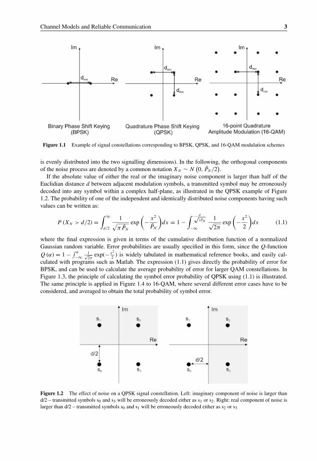
In the following examples, we consider digital data which is mapped to binary phase shift keying(BPSK), quaternary phase shift keying (QPSK/4-QAM), and 16-point quadrature amplitude modulation(16-QAM) symbols. We consider complex baseband signals, that is, for our purposes the transmittedmodulation symbols corresponding to a given digital modulation scheme are represented simply ascomplex numbers. The constellation diagrams for these examples are illustrated in Figure 1.1. The effectof an AWGN channel is to shift these numbers in the complex plane. The receiver has to decide, basedon an observed shifted complex number, the most likely transmitted symbol. This decision is performedby finding which, out of the set of known transmitted symbols, is the one with the smallest Euclidiandistance to the received noisy symbol. This is a rather abstract representation of digital signals and noise,but sufficient for performing error performance analyses of different modulation schemes. For a moredetailed discussion on basic modulation methods and the corresponding signal forms, see Chapter 2.

As outlined above, in complex baseband signal-space representations, the effect of additive whiteGaussian noise in the receiver can be described as a complex number added to each transmitted mod-ulation symbol value. The real and imaginary parts of these complex numbers are independent andidentically distributed Gaussian random variables with zero mean and variance equal to σ 2

N = P̄N /2,where P̄N denotes the total average power of the complex noise process (that is, the power of the noise

P1: TIX/XYZ P2: ABC


Channel Models and Reliable Communication 3

Figure 1.1 Example of signal constellations corresponding to BPSK, QPSK, and 16-QAM modulation schemes

is evenly distributed into the two signalling dimensions). In the following, the orthogonal componentsof the noise process are denoted by a common notation X N ∼ N

(0, P̄N /2

).

If the absolute value of either the real or the imaginary noise component is larger than half of theEuclidian distance d between adjacent modulation symbols, a transmitted symbol may be erroneouslydecoded into any symbol within a complex half-plane, as illustrated in the QPSK example of Figure1.2. The probability of one of the independent and identically distributed noise components having suchvalues can be written as:

P (X N > d/2) =∫ ∞

d/2

1√

π P̄N

exp

(− x2

P̄N

)dx = 1 −

∫ d√2P̄N

−∞

1√2π

exp

(− x2

2

)dx (1.1)

where the final expression is given in terms of the cumulative distribution function of a normalizedGaussian random variable. Error probabilities are usually specified in this form, since the Q-functionQ (α) = 1 − ∫ α

−∞1√2π

exp(− x2

2 ) is widely tabulated in mathematical reference books, and easily cal-culated with programs such as Matlab. The expression (1.1) gives directly the probability of error forBPSK, and can be used to calculate the average probability of error for larger QAM constellations. InFigure 1.3, the principle of calculating the symbol error probability of QPSK using (1.1) is illustrated.The same principle is applied in Figure 1.4 to 16-QAM, where several different error cases have to beconsidered, and averaged to obtain the total probability of symbol error.

Figure 1.2 The effect of noise on a QPSK signal constellation. Left: imaginary component of noise is larger thand/2 – transmitted symbols s0 and s3 will be erroneously decoded either as s1 or s2. Right: real component of noise islarger than d/2 – transmitted symbols s0 and s1 will be erroneously decoded either as s2 or s3

P1: TIX/XYZ P2: ABC



Figure 1.3 Principle of calculating the probability of symbol error for a QPSK signal constellation, assuming s0 istransmitted. Left: 2P(XN > d/2) includes twice the probability of receiving a value in the diagonally opposite quadrant.Right 2P(XN > d/2)- P(XN > d/2)2 is the correct probability of symbol error

In the preceeding examples, the error probabilities are calculated in terms of the minimum distanceof the constellations and the average noise power. However, it is more convenient to consider errorprobabilities in terms of the ratio of average signal and noise powers. For any uniform QAM constellation,the distance between any pair of neighbouring symbols (that is, the minimum distance) is easily obtainedas a function of the average transmitted signal power P̄S – which is calculated as the average over thesquared absolute values of the complex-valued constellation points – as:

d =

⎧⎪⎪⎨

⎪⎪⎩

2√

P̄S

2√

P̄S/2

2√

P̄S/10

(BPSK)

(QPSK)

(16 − QAM)

The average symbol error probability for each of the cases above is now obtained by calculating averagesover demodulation error probabilities for the signal sets as a function of the average signal-to-noiseratio, given by P̄S/P̄N =̂λ. Using the equations given above, the average symbol error probabilities are

Figure 1.4 Principle of calculating the probability of symbol error for a 16-QAM signal constellation. Left: forthe four corner symbols, the probability of symbol error is 2P(XN > d/2)-P(XN > d/2)2. Center: for the eight outersymbols, 3P(XN > d/2)-2P(XN > d/2)2. Right: for the middle symbols, 4P(XN > d/2)-4P(XN > d/2)2. The totalprobability of symbol error is the weighted average of these probabilities

P1: TIX/XYZ P2: ABC



obtained, following the principle outlined in the examples of Figures 1.3 and 1.4, as:

ps (λ) =

⎧⎪⎪⎪⎨

⎪⎪⎪⎩

Q(√

2λ)

2Q(√

λ)

− Q(√

λ)2

3Q(√

λ/5)

− 9

4Q

(√λ/5

)2

(BPSK)(QPSK)

(16 − QAM)

1.2.2 From Sample SNR to Eb/N0

Assume the transmitted symbols are mapped to rectangular baseband signal pulses of duration Tsymb,sampled with frequency fsampl, with complex envelopes corresponding to the constellation points of thesignal-space representation used above. These rectangular pulses are then modulated by a given carrierfrequency, transmitted through a noisy channel, downconverted in a receiver and passed to a matchedfilter or correlator for signal detection.

Figure 1.5 shows an example of two BPSK symbols transmitted and received as described above. Inthis example, the signal-to-noise ratio per sample is defined as SNR = A2/σ n

2, where σ n2 is the sample

variance of the real-valued noise process. It can be seen that, based on any individual sample of thereceived signals, the probability of error is quite large. However, calculating the averages (plotted withdashed lines in Figure 1.5) of the signals over their entire durations (0.1 s, containing 100 samples) givesvalues for the signal envelopes that are very close to the correct values −1 and 1, thus reducing the effectof the added noise considerably. It is clear that in this case, the sample SNR is no longer enough todetermine the probability of error at the receiver. The relevant question is how should the sample SNRbe scaled to obtain the correct error probability? We study this using BPSK as an example.

Figure 1.5 Two noisy signal envelopes and their averages. For this example, Tsymb = 0.1 s, fsampl= 1000 Hz, A1 =–A0 = 1, Eb/N0 = 15 dB ↔ SNR = –5 dB

P1: TIX/XYZ P2: ABC



As above, the probability of symbol (bit) error based on the signal-space representation for BPSKover an AWGN channel is:

Pe = P (N < −A1) =∫ −A1

−∞

1

σn

√2π

exp

(− x2

2σ 2n

)dx

where N is a normally distributed random variable with standard deviation σ n and zero mean, and it isassumed (without loss of generality) that the signal amplitude A1 > 0 (corresponding to a 1 being sent).This can be thought of as transmitting a single sample of the signal envelope. Sampling a received signalenvelope S(t) + N(t) at k points produces a sequence of samples S(i·Tsampl) + N(i·Tsampl), where Tsampl =1/fsampl, and i = 1. . .k. A correlator receiver for BPSK may use the following test statistic to decidewhether a 1 was most likely to be transmitted:

Z = A1

(k∑

i=1

(S

(i · Tsampl

) + N(i · Tsampl

)))

=k∑

i=1

(A1 S

(i · Tsampl

)) +k∑

i=1

(A1 N

(i · Tsampl

))

Assuming that a 1 was indeed sent, a false decision will be made if:

A1

k∑

i=1

N(i · Tsampl

)< −k · A2

1 ⇔ 1

kN

(i · Tsampl

)< −A1

or

N̄ < −A1

denoting the sample mean of the noise as N̄ . We note that the expression is the same as for the singlesample case, only with the normal random variable replaced by the sample mean of k samples from anormal distribution. Basic results of statistics state that this sample mean is also normally distributed, inthis case with mean zero and standard deviation σN̄ = σn/

√k. We thus find that the error probability in

this example is determined by the ratio k · (σ 2s /σ 2

n ), or k times the sample SNR.It should be noted that although we used BPSK as an example to simplify the relevant expressions,

the above result is not restricted only to BPSK. In fact, the obtained expression k · (σ 2s /σ 2

n ) is generallyused in a form derived as follows:

k · σ 2s

σ 2n

= Tsymb

Tsampl· P̄S

P̄N= P̄S · Tsymb(

1/ fsampl) · N0 Bn

= ES

N0

In the above, N0 is the noise power spectral density and Bn is the noise bandwidth. Note that the signalenergy ES = P̄S · Tsymb, and that Bn = fsampl (this is based on the Shannon-Nyquist sampling theoremapplied for complex samples). Note also that here it is implicitly assumed that the signal bandwidthcorresponds to the Nyquist frequency; if the signal is oversampled, care should be taken in performanceanalysis to include only the noise bandwidth which overlaps with the spectrum of the signal. Finally,the ratio of energy per bit to noise power spectral density Eb/N0, very commonly used as a measure forsignal quality, is obtained as:

Eb

N0= 1

nb

Es

N0

where nb is the number of bits per transmitted symbol.

1.3 Fading Processes in Wireless Communication ChannelsAdditive noise is present in all communication systems. It is a fundamental result of informationtheory that the ratio of signal and noise powers at the receiver determines the capacity, or maximum

P1: TIX/XYZ P2: ABC



Figure 1.6 System model for transmitting information through a channel with additive white Gaussian noise

achievable rate of error-free transmission of information, of a channel. Generally, multiplicative effectsof a communication channel, or fading, can be represented as a convolution of the transmitted signalwith the channel impulse response, as illustrated in Figure 1.6. A general effect of fading is to reduce thesignal power arriving at the receiver. Since the noise power at the receiver is independent of the usefulsignal, and the noise component does not experience fading, a fading channel generally reduces the ratioof the signal power to the noise power at the receiver, thus also reducing the transmission capacity.

The distortion, or noise, caused by a communication channel to the transmitted signal can be dividedinto multiplicative and additive components; the latter was considered above. Multiplicative noise,or fading, can be defined as the relative difference between the powers contained in correspondingsections of the transmitted and received signals. Factors that typically contribute to the fading in wirelesscommunication systems are the transmitter and receiver antenna and analog front-end characteristics,absorption of the signal power by the propagation media, and reflection, refraction, scattering anddiffraction caused by obstacles in the propagation path. The receiver experiences the combined effect ofall these physical factors, which vary according to the positions of the receiver and transmitter withinthe propagation environment. It should be noted that it is generally possible to describe the effects ofa communication channel entirely by its impulse response as illustrated in Figure 1.6. However, it istypical that estimation of the average power conveyed by a transmission channel is performed separatelyfrom the modelling of the channel’s impulse response, which is then power-normalized. We also applythis principle in the following discussion on fading processes in wireless channels.

Fading in wireless channels is in literature typically characterized as a concatenation or superpositionof several types of fading processes. These processes are often classified using the qualitative terms pathloss, shadowing, and multipath fading, which is also often referred to as fast fading. However, thesefading processes cannot in general be considered fully independent of each other, and indeed in manyreferences (for example in [1],[12]) path loss and shadowing are not considered as separate processes.Justification for this will be subsequently considered in more detail. In the following, fading is primarilyclassified according to the typical variation from the mean attenuation over a spatial region of givenmagnitude. The terms large-scale, medium-scale, and small-scale fading are thus used.

Small-scale fading corresponds directly to multipath fading, and involves signal power variations ofmagnitude up to 40 dB on a spatial scale of a half-wavelength (for example 50 cm at 300 MHz). Averagingthe total fading in the receiver over a spatial interval significantly larger than a half-wavelength providesinformation on the medium-scale fading, or shadowing. Over spatial intervals of magnitude hundreds ofmeters, medium-scale fading involves signal power variations up to magnitude 20 dB. Again, averagingthe total fading over a spatial interval of several hundred meters provides an estimate for the large-scalefading, which may vary up to 150 dB over the considered coverage area. [9] These denominations do notsuggest a different origin or effect for the fading types, but rather signify that typically different variationaround the mean attenuation is observed at different spatial scales, or observation windows.

1.3.1 Large-Scale Fading (Path Loss)

Large-scale fading, or path loss, is commonly modelled for signals at a given carrier frequency as adeterministic function of the distance between the transmitter and receiver, and is affected by several

P1: TIX/XYZ P2: ABC



parameters such as antenna gains and properties of the propagation environment between the transmitterand receiver. Main physical factors that contribute to large-scale fading are free-space loss, or thedispersion of the transmitted signal power into surrounding space, plane earth loss, and absorption of thesignal power by the propagation medium.

Free-space loss corresponds to dispersion of transmitted signal power into the space surrounding thetransmitter antenna. The most simple free-space loss estimation is obtained by assuming that signalsare transmitted omnidirectionally, that is, power is radiated equally to all directions, and there are noobstacles within or around the transmission area, which would affect the propagation of electromagneticsignals. With such assumptions, the power density at a distance d meters from the transmitter can bewritten as:

pR = PT

4πd2(watts/m2)

where PT is the total transmitted signal power. This expression is obtained simply by dividing thetransmitted power over the surface area of a sphere surrounding the transmitter antenna.

The assumptions specified above are not practical in most communication scenarios. Ignoring for nowthe likely presence of obstacles around the transmitter and receiver, the free-space loss defined abovecan be modified into a more realistic expression by taking into account the antenna characteristics of thetransmitter and receiver. Specifically, the actual received power depends on the effective aperture areaof the receiver antenna, which can be written as:

AR = λ2G R

4π(m2)

where λ is the wavelength of the transmitted signal and GR is the receiver antenna gain, which is affectedby the directivity of the antenna – specifically the antenna radiation patterns in the direction of thearriving signal. It should be noted that the above expression means that the received power decreasesalong with an increase in the carrier frequency. Finally, taking into account the transmitter antenna gainfactor GT, the received power after free-space loss can be written as:

PR = GT pR AR = PT GT G Rλ2

(4πd)2(W)

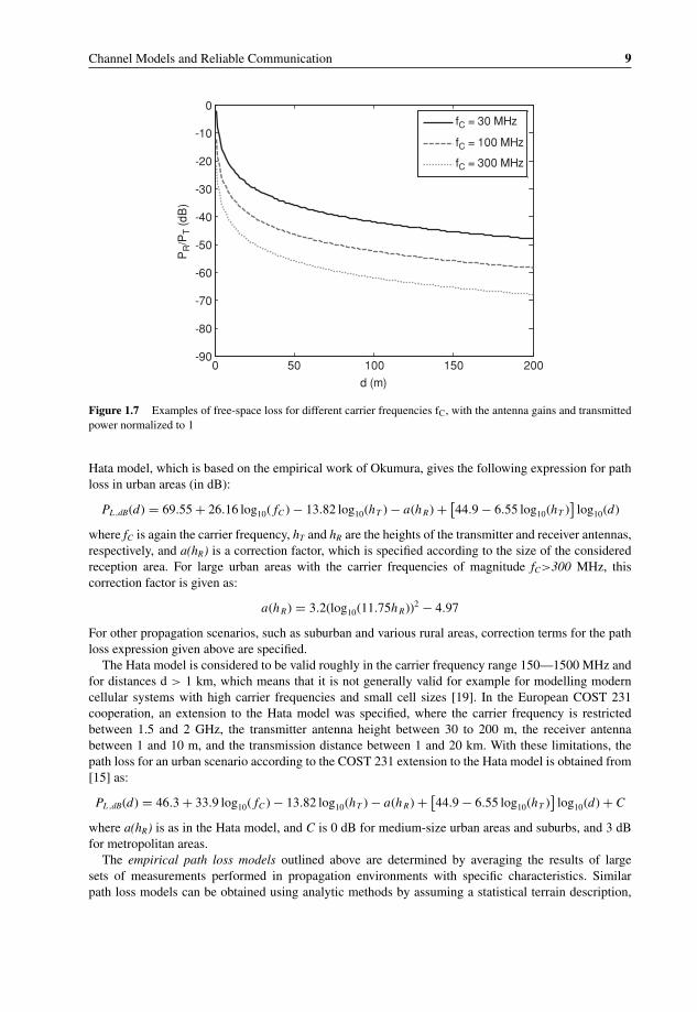
Note that in the above, the variables are assumed to be given in the linear scale, that is, not in decibels.Figure 1.7 shows examples of the received power as a function of distance from the transmitted antennafor different carrier frequencies, with the antenna gains and transmitted signal power normalized tounity. Formally, an expression for the path loss PL, that is, attenuation of the transmitted signal, isobtained from the above in decibels as:

PL ,dB = 10 log10

PT

PR=10 log10

(4πd)2

GT G Rλ2= 20 log10(4πd) − 10 log10(GT ) − 10 log10(G R) − 20 log10(λ)

Real signals do not follow the simple free-space attenuation model partly due to the presence of theground plane close to the transmitter and receiver. This causes so called plane earth loss, where signalcomponents reflected from the ground plane destructively interfere with the received useful signal. Theamount of plane earth loss depends on the distance and heights of the transmitter and receiver antennas.Another significant cause for attenuation is the absorption of signal power by atmospheric gases andhydrometeors (such as clouds, rain, snow etc.).

In addition to these factors, large-scale fading is typically defined to include the average of theshadowing and multipath fading effects. Thus the type of propagation environment must be taken intoaccount in the total power loss. This has been done for example in the widely used Okumura-Hata[13],[14] and COST 231 [15] models by approximating the parameters for the propagation loss forspecific environments and transmission setups from sets of field measurements [1]. As an example, the

P1: TIX/XYZ P2: ABC



0 50 100 150 200-90

-80

-70

-60

-50

-40

-30

-20

-10

0

d (m)

PR/P

T (d

B)

fC = 30 MHz

fC = 100 MHz

fC = 300 MHz

Figure 1.7 Examples of free-space loss for different carrier frequencies fC, with the antenna gains and transmittedpower normalized to 1

Hata model, which is based on the empirical work of Okumura, gives the following expression for pathloss in urban areas (in dB):

PL ,dB(d) = 69.55 + 26.16 log10( fC ) − 13.82 log10(hT ) − a(h R) + [44.9 − 6.55 log10(hT )

]log10(d)

where fC is again the carrier frequency, hT and hR are the heights of the transmitter and receiver antennas,respectively, and a(hR) is a correction factor, which is specified according to the size of the consideredreception area. For large urban areas with the carrier frequencies of magnitude fC>300 MHz, thiscorrection factor is given as:

a(h R) = 3.2(log10(11.75h R))2 − 4.97

For other propagation scenarios, such as suburban and various rural areas, correction terms for the pathloss expression given above are specified.

The Hata model is considered to be valid roughly in the carrier frequency range 150—1500 MHz andfor distances d > 1 km, which means that it is not generally valid for example for modelling moderncellular systems with high carrier frequencies and small cell sizes [19]. In the European COST 231cooperation, an extension to the Hata model was specified, where the carrier frequency is restrictedbetween 1.5 and 2 GHz, the transmitter antenna height between 30 to 200 m, the receiver antennabetween 1 and 10 m, and the transmission distance between 1 and 20 km. With these limitations, thepath loss for an urban scenario according to the COST 231 extension to the Hata model is obtained from[15] as:

PL ,dB(d) = 46.3 + 33.9 log10( fC ) − 13.82 log10(hT ) − a(h R) + [44.9 − 6.55 log10(hT )

]log10(d) + C

where a(hR) is as in the Hata model, and C is 0 dB for medium-size urban areas and suburbs, and 3 dBfor metropolitan areas.

The empirical path loss models outlined above are determined by averaging the results of largesets of measurements performed in propagation environments with specific characteristics. Similarpath loss models can be obtained using analytic methods by assuming a statistical terrain description,

P1: TIX/XYZ P2: ABC



where obstacles of suitable geometry are distributed randomly in the propagation environment, andby calculating the average propagation loss based on such approximations. For example, [11] containsa detailed description of deriving functions for path loss in various land environments using analyticmethods. The physical mechanisms that cause the environment-specific propagation loss are the samefor large-scale fading as for medium-scale fading, and are considered in more detail shortly.

Deterministic large-scale fading models – where estimations of the path loss are obtained as functionsof the propagation distance – are useful in applications where it is sufficient to have rough estimates onthe average attenuation of signal power over a large transmission area, or it is impractical to approximatesignal attenuation in more detail. These models are typically used for example in radio resource manage-ment and planning of large wireless networks. It should be noted that expressions for large-scale fadingcan be obtained for generic environments using statistical methods as outlined above or for specifictransmission sites by averaging over a site-specific approximation of medium-scale fading. However,this is typically a computationally involved task, as described in the following.

1.3.2 Medium-Scale Fading (Shadowing)

As with large-scale fading, methods for modelling medium-scale fading can typically be categorized asstatistical or site-specific. In the statistical approach, the fading is typically assumed – based on empiricaldata – to follow a lognormal distribution. The mean for this distribution can be obtained for a given carrierfrequency and distance from the transmitter using expressions for large-scale fading as outlined in theprevious subsection. The standard deviation and autocorrelation of the lognormal distribution are modelparameters, which must be selected according to the propagation environment. This standard deviationis known as the location variability, and it determines the range of fluctuation of the signal field strengtharound the mean value. Its value increases with frequency, and is also dependent on the propagationscenario – for example, the standard deviation is typically larger in suburban areas than in open areas.The standard deviation is typically in the range of 5 to 12 dB. Spatial correlation of shadowing is usuallymodelled using a first-order exponential model [20]:

ρ(d) = e−d/dcorr

where dcorr is the distance over which the correlation is reduced by e−1. This distance is typically of thesame order as the sizes of blocking objects or object clusters within the transmission area.

An intuitive justification for the applicability of a lognormal model for medium-scale, or shadow fading,can be obtained by considering the total attenuation of the signal components arriving at the receiver inan environment with a large number of surrounding obstacles. Typically the signal components arrivingat the receiver have passed through a number of obstacles of random dimensions, each attenuating thesignal power by some multiplicative factor. The product of these fading factors contributes to the totalpower attenuation. In the logarithmic scale, the product of several fading components is represented asthe sum of their logarithms, and again according to the central limit theorem the distribution of this sumapproaches a normal distribution. Figure 1.8 shows examples of log-normal medium-scale fading forstandard deviation 10 dB, and correlation distances 20 and 50 meters.

If site-specific data on the terrain profile and obstructions along the propagation path from the trans-mitter to the receiver are available, an approximation for medium-scale fading can be calculated assummarized in [9]:

1. Locate the positions and heights of the antennas.2. Construct the great circle – or geodesic – path between the antennas. This represents the shortest

distance between the two terminals measured across the Earth’s surface.3. Derive the terrain path profile. These are readily obtained from digital terrain maps, but it is of course

also possible to use traditional contour profile maps.

do not print pantone 032 red guidelines. for...

Documents