Finance and Economics Discussion Series Divisions of Research & Statistics and Monetary Affairs

Federal Reserve Board, Washington, D.C.

Do Macro Variables, Asset Markets, or Surveys Forecast Inflation Better?

Andrew Ang, Geert Bekaert, and Min Wei 2006-15

NOTE: Staff working papers in the Finance and Economics Discussion Series (FEDS) are preliminary materials circulated to stimulate discussion and critical comment. The analysis and conclusions set forth are those of the authors and do not indicate concurrence by other members of the research staff or the Board of Governors. References in publications to the Finance and Economics Discussion Series (other than acknowledgement) should be cleared with the author(s) to protect the tentative character of these papers.

Do Macro Variables, Asset Markets, or SurveysForecast Inflation Better?∗

Andrew Ang†

Columbia University and NBER

Geert Bekaert‡

Columbia University, CEPR and NBER

Min Wei§

Federal Reserve Board of Governors

This Version: 13 February, 2006

JEL Classification: E31, E37, E43, E44Keywords: ARIMA, Phillips curve,

forecasting, term structure models, Livingston

∗We thank Jean Boivin for kindly providing data. Andrew Ang acknowledges support from theNational Science Foundation. We have benefitted from the comments of Todd Clark, Dean Croushore,Bob Hodrick, Jonas Fisher, Robin Lumsdaine, Michael McCracken, Antonio Moreno, Serena Ng, andTom Stark, and seminar participants at Columbia Universityand Goldman Sachs Asset Management.We especially thank the editor, Charles Plosser, and an anonymous referee for excellent comments. Theopinions expressed in this paper do not necessarily reflect those of the Federal Reserve Board or theFederal Reserve system.

†Columbia Business School, 805 Uris Hall, 3022 Broadway, NewYork, NY 10027; ph: (212) 854-9154; fax: (212) 662-8474; email: aa610@columbia.edu; WWW: http://www.columbia.edu/∼aa610

‡Columbia Business School, 802 Uris Hall, 3022 Broadway, NewYork, NY 10027; ph: (212) 854-9156; fax: (212) 662-8474; email: gb241@columbia.edu; WWW: http://www.gsb.columbia.edu/fac-ulty/gbekaert

§Federal Reserve Board of Governors, Division of Monetary Affairs, Washington, DC 20551; ph:(202) 736-5619; fax: (202) 452-2301; email: min.wei@frb.gov; WWW: www.federalreserve.gov/re-search/staff/weiminx.htm

Abstract

Surveys do! We examine the forecasting power of four alternative methods of forecasting U.S.

inflation out-of-sample: time-series ARIMA models; regressions using real activity measures

motivated from the Phillips curve; term structure models that include linear, non-linear, and

arbitrage-free specifications; and survey-based measures. We also investigate several methods

of combining forecasts. Our results show that surveys outperform the other forecasting methods

and that the term structure specifications perform relatively poorly. We find little evidence that

combining forecasts produces superior forecasts to surveyinformation alone. When combining

forecasts, the data consistently places the highest weights on survey information.

1 Introduction

Obtaining reliable and accurate forecasts of future inflation is crucial for policymakers conduct-

ing monetary and fiscal policy; for investors hedging the risk of nominal assets; for firms making

investment decisions and setting prices; and for labor and management negotiating wage con-

tracts. Consequently, it is no surprise that a considerableacademic literature evaluates different

inflation forecasts and forecasting methods. In particular, economists use four main methods

to forecast inflation. The first method is atheoretical, using time series models of the ARIMA

variety. The second method builds on the economic model of the Phillips curve, leading to

forecasting regressions that use real activity measures. Third, we can forecast inflation using

information embedded in asset prices, in particular the term structure of interest rates. Finally,

survey-based measures use information from agents (consumers or professionals) directly to

forecast inflation.

In this article, we comprehensively compare and contrast the ability of these four methods

to forecast inflation out of sample. Our approach makes four main contributions to the litera-

ture. First, our analysis is the first to comprehensively compare the four methods: time-series

forecasts, forecasts based on the Phillips curve, forecasts from the yield curve, and all three

available surveys (the Livingston, Michigan, and SPF surveys). The previous literature has

concentrated on only one or two of these different forecasting methodologies. For example,

Stockton and Glassman (1987) show that pure time-series models out-perform more sophisti-

cated macro models, but do not consider term structure models or surveys. Fama and Gibbons

(1984) compare term structure forecasts with the Livingston survey, but they do not consider

forecasts from macro factors. Whereas Grant and Thomas (1999), Thomas (1999) and Mehra

(2002) show that surveys out-perform simple time-series benchmarks for forecasting inflation,

none of these studies compares the performance of survey measures with forecasts from Phillips

curve or term structure models.

The lack of a study comparing these four methods of inflation forecasting implies that there

is no well-accepted set of findings regarding the superiority of a particular forecasting method.

The most comprehensive study to date, Stock and Watson (1999), finds that Phillips curve-

based forecasts produce the most accurate out-of-sample forecasts of U.S. inflation compared

with other macro series and asset prices, using data up to 1996. However, Stock and Watson

only briefly compare the Phillips-curve forecasts to the Michigan survey and to simple regres-

sions using term structure information. Stock and Watson donot consider no-arbitrage term

structure models, non-linear forecasting models, or combined forecasts from all four forecast-

1

ing methods. Recent work also casts doubts on the robustnessof the Stock-Watson findings. In

particular, Atkeson and Ohanian (2001), Fisher, Liu and Zhou (2002), Sims (2002), and Cec-

chetti, Chu and Steindel (2000), among others, show that theaccuracy of Phillips curve-based

forecasts depends crucially on the sample period. Clark andMcCracken (2006) address the

issue of how instability in the output gap coefficients of thePhillips curve affects forecasting

power. To assess the stability of the inflation forecasts across different samples, we consider

out-of-sample forecasts over both the post-1985 and post-1995 periods.

Our second contribution is to evaluate inflation forecasts implied by arbitrage-free asset

pricing models. Previous studies employing term structuredata mostly use only the term spread

in simple OLS regressions and usually do not use all available term structure data (see, for

example, Mishkin, 1990, 1991; Jorion and Mishkin, 1991; Stock and Watson, 2003). Frankel

and Lown (1994) use a simple weighted average of different term spreads, but they do not

impose no-arbitrage restrictions. In contrast to these approaches, we develop forecasting models

that use all available data and impose no-arbitrage restrictions. Our no-arbitrage term structure

models incorporate inflation as a state variable because inflation is an integral component of

nominal yields. The no-arbitrage framework allows us to extract forecasts of inflation from

data on inflation and asset prices taking into account potential time-varying risk premia.

No-arbitrage constraints are reasonable in a world where hedge funds and investment banks

routinely eliminate arbitrage opportunities in fixed income securities. Imposing theoretical no-

arbitrage restrictions may also lead to more efficient estimation. Just as Ang, Piazzesi and Wei

(2004) show that no-arbitrage models produce superior forecasts of GDP growth, no-arbitrage

restrictions may also produce more accurate forecasts of inflation. In addition, this is the first ar-

ticle to investigate non-linear, no-arbitrage models of inflation. We investigate both an empirical

regime-switching model incorporating term structure information and a no-arbitrage, non-linear

term structure model following Ang, Bekaert and Wei (2006) with inflation as a state variable.

Our third contribution is that we thoroughly investigate combined forecasts. Stock and Wat-

son (2002a, 2003), among others, show that the use of aggregate indices of many macro series

measuring real activity produces better forecasts of inflation than individual macro series. To

investigate this further, we also include the (Phillips curve-based) index of real activity con-

structed by Bernanke, Boivin and Eliasz (2005) from 65 macroeconomic series. In addition,

several authors (see, e.g., Stock and Watson, 1999; Brave and Fisher, 2004; Wright, 2004)

advocate combining several alternative models to forecastinflation. We investigate five differ-

ent methods of combining forecasts: simple means or medians, OLS based combinations, and

Bayesian estimators with equal or unit weight priors.

2

Finally, our main focus is forecasting inflation rates. Because of the long-standing debate in

macroeconomics on the stationarity of inflation rates, we also explicitly contrast the predictive

power of some non-stationary models to stationary models and consider whether forecasting

inflation changes alters the relative forecasting ability of different models.

Our major empirical results can be summarized as follows. The first major result is that sur-

vey forecasts outperform the other three methods in forecasting inflation. That the median Liv-

ingston and SPF survey forecasts do well is perhaps not surprising, because presumably many

of the best analysts use time-series and Phillips Curve models. However, even participants in the

Michigan survey who are consumers, not professionals, produce accurate out-of-sample fore-

casts, which are only slightly worse than those of the professionals in the Livingston and SPF

surveys. We also find that the best survey forecasts are the survey median forecasts themselves;

adjustments to take into account both linear and non-linearbias yield worse out-of-sample fore-

casting performance.

Second, term structure information does not generally leadto better forecasts and often leads

to inferior forecasts than models using only aggregate activity measures. Whereas this confirms

the results in Stock and Watson (1999), our investigation ofterm structure models is much

more comprehensive. The relatively poor forecasting performance of term structure models

extends to simple regression specifications, iterated long-horizon VAR forecasts, no-arbitrage

affine models, and non-linear no-arbitrage models. These results suggest that while inflation is

very important for explaining the dynamics of the term structure (see, e.g., Ang, Bekaert and

Wei, 2006), yield curve information is less important for forecasting future inflation.

Our third major finding is that combining forecasts does not generally lead to better out-of-

sample forecasting performance than single forecasting models. In particular, simple averaging,

like using the mean or median of a number of forecasts, does not necessarily improve the fore-

cast performance, whereas linear combinations of forecasts with weights computed based on

past performance and prior information generate the biggest gains. Even the Phillips curve

models using the Bernanke, Boivin and Eliasz (2005) forward-looking aggregate measure of

real activity mostly does not perform well relative to simpler Phillips curve models and never

outperforms the survey forecasts. The strong success of thesurveys in forecasting inflation out-

of-sample extends to surveys dominating other models in forecast combinination methods. The

data consistently place the highest weights on the survey forecasts and little weight on other

forecasting methods.

The remainder of this paper is organized as follows. Section2 describes the data set. In

Section 3, we describe the time-series models, predictive macro regressions, term structure

3

models, and forecasts from survey data, and detail the forecasting methodology. Section 4

contains the empirical out-of-sample results. We examine the robustness of our results to a

non-stationary inflation specification in Section 5. Finally, Section 6 concludes.

2 Data

2.1 Inflation

We consider four different measures of inflation. The first three are consumer price index (CPI)

measures, including CPI-U for All Urban Consumers, All Items (PUNEW), CPI for All Ur-

ban Consumers, All Items Less Shelter (PUXHS) and CPI for All Urban Consumers, All Items

Less Food and Energy (PUXX), which is also called core CPI. The latter two measures strip

out highly volatile components in order to better reflect underlying price trends (see the discus-

sion in Quah and Vahey, 1995). The fourth measure is the Personal Consumption Expenditure

deflator (PCE). While all three surveys forecast a CPI-based inflation measure, PCE inflation

features prominently in policy work at the Federal Reserve.All measures are seasonally ad-

justed and obtained from the Bureau of Labor Statistics website. The sample period is 1952:Q2

to 2002:Q4 for PUNEW and PUXHS, 1958:Q2 to 2002:Q4 for PUXX, and 1960:Q2 to 2002:Q4

for PCE.

We define the quarterly inflation rate,πt, from t− 1 to t as:

πt = ln

(Pt

Pt−1

), (1)

wherePt is the level of one of the four inflation indices at timet. We use the terms “inflation”

and “inflation rate” interchangeably as defined in equation (1). We take one quarter to be our

base unit for estimation purposes, but forecast annual inflation,πt+4,4, from t to t+ 4:

πt+4,4 = πt+1 + πt+2 + πt+3 + πt+4, (2)

whereπt is the quarterly inflation rate in equation (1).

Empirical work on inflation has failed to come to a consensus regarding its stationarity

properties. For example, Bryan and Cecchetti (1993) assumea stationary inflation process,

while Nelson and Schwert (1977) and Stock and Watson (1999) assume that the inflation process

has a unit root. Most of our analysis assumes that inflation isstationary for two reasons. First,

it is difficult to generate non-stationary inflation in standard economic models, whether they

are monetary in nature, or of the New Keynesian variety (see Fuhrer and Moore, 1995; Holden

4

and Driscoll, 2003). Second, the working paper version of Bai and Ng (2004) recently rejects

the null of non-stationarity for inflation. That being said,Cogley and Sargent (2005) and Stock

and Watson (2005) find evidence of changes in inflation persistence over time, with a random

walk or integrated MA-process providing an accurate description of inflation dynamics during

certain times. Furthermore, the use of a parsimonious non-stationary model may be attractive

for forecasting. In particular, Atkeson and Ohanian (2001)have made the random walk a natural

benchmark to beat in forecasting exercises. Therefore, we consider whether our results are

robust to assuming non-stationary inflation in Section 5.

Table 1 reports summary statistics for all four measures of inflation for the full sample in

Panel A, and the post-1985 sample and the post-1995 sample inPanels B and C, respectively.

Our statistics pertain to annual inflation,πt+4,t, but we sample the data quarterly. Therefore, we

report the fourth autocorrelation for quarterly inflation,which corresponds to the first autocor-

relation for annual inflation. Table 1 shows that all four inflation measures are lower and more

stable during the last two decades, in common with many othermacroeconomic series, includ-

ing output (see Kim and Nelson, 1999; McConnell and Perez-Quiros, 2000; Stock and Watson,

2002b). Core CPI (PUXX) has the lowest volatility of all the inflation measures. PUXX volatil-

ity ranges from 2.56% per annum over the full sample to only 0.24% per annum post-1996. The

higher variability of the other measures in the latter part of the sample must be due to food and

energy price changes. In the later sample periods, PCE inflation is, on average, lower than CPI

inflation, which may be partly due to its use of a chain weighting in contrast to the other CPI

measures which use a fixed basket (see Clark, 1999).

Inflation is somewhat persistent (0.79% for PUNEW over the full sample), but its persistence

decreases over time, as can be seen from the lower autocorrelation coefficients for the PUNEW

and the PUXHS measures after 1986, and for all measures after1995. The correlations of

the four measures of inflation with each other are all over 75%over the full sample. The

comovement can be clearly seen in the top panel of Figure 1. Inflation is lower prior to 1969 and

after 1983, but reaches a high of around 14% during the oil crisis of 1973–1983. PUXX tracks

both PUNEW and PUXHS closely, except during the 1973–1975 period, where it is about 2%

lower than the other two measures, and after 1985, where it appears to be more stable than the

other two measures. During the periods when inflation is decelerating, such as in 1955–1956,

1987–1988, 1998–2000 and most recently 2002–2003, PUNEW declines more gradually than

PUXHS, suggesting that housing prices are less volatile than the prices of other consumption

goods during these periods.

5

2.2 Real Activity Measures

We consider six individual series for real activity along with one composite real activity factor.

We compute GDP growth (GDPG) using the seasonally adjusted data on real GDP in billions

of chained 2000 dollars. The unemployment rate (UNEMP) is also seasonally adjusted and

computed for the civilian labor force aged 16 years and over.Both real GDP and the unem-

ployment rate are from the Federal Reserve Economic Data (FRED) database. We compute

the output gap either as the detrended log real GDP by removing a quadratic trend as in Gali

and Gertler (1999), which we termGAP1, or by using the Hodrick-Prescott (1997) filter (with

the standard smoothness parameter of 1,600), which we termGAP2. At time t, both measures

are constructed using only current and past GDP values, so the filters are run recursively. We

also use the labor income share (LSHR), defined as the ratio of nominal compensation to total

nominal output in the U.S. nonfarm business sector. We use two forward-looking indicators:

the Stock-Watson (1989) Experimental Leading Index (XLI) and their Alternative Nonfinancial

Experimental Leading Index-2 (XLI-2).

Because Stock and Watson (2002a), among others, show that aggregating the information

from many factors has good forecasting power, we also use a single factor aggregating the in-

formation from 65 individual series constructed by Bernanke, Boivin and Eliasz (2005). This

single real activity series, which we termFAC, aggregates real output and income, employ-

ment and hours, consumption, housing starts and sales, realinventories, and average hourly

earnings. The sample period for all the real activity measures is 1952:Q2 to 2001:Q4, except

the Bernanke-Boivin-Eliasz real activity factor, which spans 1959:Q1 to 2001:Q3. We use the

composite real activity factor at the end of each quarter forforecasting inflation over the next

year.1

The real activity measures have the disadvantage that they may use information that is not

actually available at the time of the forecast, either through data revisions, or because of full

sample estimation in the case of the Bernanke-Boivin-Eliasz measure. This biases the forecasts

from Phillips curve models to be better than what could be actually forecasted using a real-time

data set. The use of real time economic activity measures produces much worse forecasts of

1To achieve stationarity of the underlying individual macroseries, various transformations are employed by

Bernanke, Boivin and Eliasz (2005). In particular, many series are first differenced at a monthly frequency. Better

forecasting results might be potentially obtained by taking a long 12-month difference to forecast annual inflation

(see comments by, among others, Plosser and Schwert, 1978),or pre-screening the variables to be used in the

construction of the composite factor (see Boivin and Ng, 2006). We do not consider these adjustments and use the

original Bernanke-Boivin-Eliasz series.

6

future inflation compared to the use of revised economic series in Orphanides and van Norden

(2001) but only slightly worse forecasts for both inflation and real activity in Bernanke and

Boivin (2003). Nevertheless, our forecast errors using real activity measures are likely biased

downwards.

2.3 Term Structure Data

The term structure variables are zero-coupon yields for thematurities of 1, 4, 8, 12, 16, and

20 quarters from CRSP spanning 1952:Q2 to 2001:Q4. The one-quarter rate is from the CRSP

Fama risk-free rate file, while all other bond yields are fromthe CRSP Fama-Bliss discount

bond file. All yields are continuously compounded and expressed at a quarterly frequency. We

define the short rate (RATE) to be the one-quarter yield and define the term spread (SPD) to

be the difference between the 20-quarter yield and the shortrate. Some of our term structure

models also use four-quarter and 12-quarter yields for estimation.

2.4 Surveys

We examine three inflation expectation surveys: the Livingston survey, the Survey of Profes-

sional Forecasters (SPF), and the Michigan survey.2 The Livingston survey is conducted twice a

year, in June and in December, and polls economists from industry, government, and academia.

The Livingston survey records participants’ forecasts of non-seasonally-adjusted CPI levels six

and twelve months in the future and is usually conducted in the middle of the month. Unlike

the Livingston survey, participants in the SPF and the Michigan survey forecast inflation rates.

Participants in the SPF are drawn primarily from business, and forecast changes in the quar-

terly average of seasonally-adjusted CPI-U levels. The SPFis conducted in the middle of every

quarter and the sample period for the SPF median forecasts isfrom 1981:Q3 to 2002:Q4. In

contrast to the Livingston survey and SPF, the Michigan survey is conducted monthly and asks

households, rather than professionals, to estimate expected price changes over the next twelve

months. We use the median Michigan survey forecast of inflation over the next year at the end

of each quarter from 1978:Q1 to 2002:Q4.

2We obtain data for the Livingston survey and SPF data from thePhiladelphia Fed website (http://www.phil.frb.

org/econ/liv and http://www.phil.frb.org/econ/spf, respectively). We take the Michigan survey data from the St.

Louis Federal Reserve FRED database (http://research.stlouisfed.org/fred2/series/MICH/). Median Michigan sur-

vey data is also available from the University of Michigan’swebsite (http://www.sca.isr.umich.edu/main.php.

However, there are small discrepancies between the two sources before September 1996. We choose to use data

from FRED because it is consistent with the values reported in Curtin (1996).

7

There are some reporting lags between the time the surveys are taken and the public dis-

semination of their results. For the Livingston and the SPF surveys, there is a lag of about one

week between the due date of the survey and their publication. However, these reporting lags

are largely inconsequential for our purposes. What mattersis the information set used by the

forecasters in predicting future inflation. Clearly, survey forecasts must use less up to date in-

formation than either macro-economic or term structure forecasts. For example, the Livingston

survey forecasters presumably use information up to at mostthe beginning of June and Decem-

ber, and mostly do not even have the May and November official CPI numbers available when

making a forecast. The SPF forecasts can only use information up to at most the middle of the

quarter and while we take the final month of the quarter for theMichigan survey, consumers do

not have up-to-date economic data available at the end of thequarter. But, for the economist

forecasting annual inflation with the surveys, all survey data is publicly available at the end of

each quarter for the SPF and Michigan surveys, and at the end of each semi-annual period for

the Livingston survey. Together with the slight data advantages present in revised, fitted macro

data, we are in fact biasing the results against survey forecasts.

The Livingston survey is the only survey available for our full sample. In the top panel of

Figure 1, which graphs the full sample of inflation data, we also include the unadjusted median

Livingston forecasts. We plot the survey forecast lagged one year, so that in December 1990,

we plot inflation from December 1989 to December 1990 together with the survey forecasts of

December 1989. The Livingston forecasts broadly track the movements of inflation, but there

are several large movements that the Livingston survey fails to track, for example the pickup in

inflation in 1956–1959, 1967–1971, 1972–1975, and 1978–1981. In the bottom panel of Fig-

ure 1, we graph all three survey forecasts of future one-yearinflation together with the annual

PUNEW inflation, where the survey forecasts are lagged one year for direct comparison. After

1981, all survey forecasts move reasonably closely together and track inflation movements rel-

atively well. Nevertheless, there are still some notable failures, like the slowdowns in inflation

in the early 1980s and in 1996.

3 Forecasting Models and Methodology

In this section, we describe the forecasting models and describe our statistical tests. In all

our out-of-sample forecasting exercises, we forecast future annual inflation. Hence, for all our

8

models, we compute annual inflation forecasts of:

Et(πt+4,4) = Et

(4∑

i=1

πt+i

), (3)

whereπt+4,4 is annual inflation fromt to t+ 4 defined in equation (2).

In Sections 3.1 to 3.4, we describe our 39 forecasting models. Table 2 contains a full nomen-

clature. Section 3.1 focuses on time-series models of inflation, which serve as our benchmark

forecasts; Section 3.2 summarizes our OLS regression models using real activity macro vari-

ables; Section 3.3 describes the term structure models incorporating inflation data; and finally,

Section 3.4 describes our survey forecasts. In Section 3.5,we define the out-of-sample periods

and list the criteria that we use to assess the performance ofout-of-sample forecasts. Finally,

Section 3.6 describes our methodology to combine model forecasts.

For all models except OLS regressions, we compute implied long-horizon forecasts from

single-period (quarterly) models. While Schorfheide (2005) shows that in theory, iterated fore-

casts need not be superior to direct forecasts from horizon-specific models, Marcellino, Stock

and Watson (2006) document the empirical superiority of iterated forecasts in predicting U.S.

macroeconomic series. For the OLS models, we compute the forecasts directly from the long-

horizon regression estimates.

3.1 Time-Series Models

ARIMA Models

If inflation is stationary, the Wold theorem suggests that a parsimonious ARMA(p, q) model

may perform well in forecasting. We consider two ARMA(p, q) models: an ARMA(1,1) model

and a pure autoregressive model withp lags, AR(p). The optimal lag length for the AR model is

recursively selected using the Schwartz criterion (BIC) onthe in-sample data. The motivation

for the ARMA(1,1) model derives from a long tradition in rational expectations macroeco-

nomics (see Hamilton, 1985) and finance (see Fama, 1975) thatmodels inflation as the sum of

expected inflation and noise. If expected inflation follows an AR(1) process, then the reduced-

form model for inflation is given by an ARMA(1,1) model. The ARMA(1,1) model also nicely

fits the slowly decaying autocorrelogram of inflation.

The specifications of the ARMA(1,1) model,

πt+1 = µ+ φπt + ψεt + εt+1, (4)

9

and the AR(p) model,

πt+1 = µ+ φ1πt + φ2πt−1 + . . .+ φpπt−p+1 + εt+1, (5)

are entirely standard. The ARMA(1,1) model is estimated by maximum likelihood, conditional

on a zero initial residual. We compute the implied inflation level forecast over the next year

expressed at a quarterly frequency. For the ARMA(1,1) model, the forecast is:

Et(πt+4,4) =1

1 − φ

[4 − φ (1 − φ4)

(1 − φ)

]µ+

φ (1 − φ4)

(1 − φ)πt +

(1 − φ4)ψ

(1 − φ)εt.

To facilitate the forecasts of annual inflation, we write theAR(p) model in first-order companion

form:

Xt+1 = A+ ΦXt + Ut+1,

where

Xt =

πt

πt−1

...

πt−p+1

, A =

µ

0...

0

, Φ =

φ1 φ2 ... φp

1 0 ... 0...

.... . .

...

0 0 ... 0

andUt =

εt

0...

0

.

Then, the forecast for the AR(p) model is given by:

Et(πt+4,4) = e′1 (I − Φ)−1(4I − Φ (I − Φ)−1

(I − Φ4

))A+ e′1Φ (I − Φ)−1

(I − Φ4

)Xt,

wheree1 is ap× 1 selection vector containing a one in the first row and zeros elsewhere.

Our third ARIMA benchmark is a random walk (RW) forecast whereπt+1 = πt + εt+1, and

Et(πt+4,4) = 4πt. Inspired by Atkeson and Ohanian (2001), we also forecast inflation using a

random walk model on annual inflation, where the forecast is given byEt(πt+4,4) = πt,4. We

denote this forecast asAORW.

Regime-Switching Models

Evans and Wachtel (1993), Evans and Lewis (1995), and Ang andBekaert (2004), among oth-

ers, document regime-switching behavior in inflation. A regime-switching model may poten-

tially account for non-linearities and structural changes, such as a sudden shift in inflation ex-

pectations after a supply shock, or a change in inflation persistence.

We estimate the following univariate regime-switching model for inflation, which we term

RGM:

πt+1 = µ (st+1) + φ (st+1)πt + σ (st+1) εt+1 (6)

10

The regime variablest = 1, 2 follows a Markov chain with constant transition probabilities

P = Pr(st+1 = 1|st = 1) andQ = Pr(st+1 = 2|st = 2). The model can be estimated using

the Bayesian filter algorithms of Hamilton (1989) and Gray (1996). We compute the implied

annual horizon forecasts of inflation from equation (6), assuming that the current regime is

the regime that maximizes the probabilityPr(st|It). This is a byproduct of the estimation

algorithm.

3.2 Regression Forecasts Based on the Phillips Curve

In standard Phillips curve models of inflation, expected inflation is linked to some measure

of the output gap. There are both forward- and backward-looking Phillips curve models, but

ultimately even forward-looking models link expected inflation to the current information set.

According to the Phillips curve, measures of real activity should be an important part of this

information set. We avoid the debate regarding the actual measure of the output gap (see, for

instance, Gali and Gertler, 1999) by taking an empirical approach and using a large number of

real activity measures. We choose not to estimate structural models because the BIC criterion

is likely to choose the empirical model best suitable for forecasting. Previous work often finds

that models with the clearest theoretical justification often have poor predictive content (see the

literature summary by Stock and Watson, 2003).

The empirical specification we estimate is:

πt+4,4 = α + β(L)′Xt + εt+4,4 (7)

whereXt combinesπt and one or two real activity measures. The lag length in the lag polyno-

mialβ(L) is selected by BIC on the in-sample data and is set to be equal across all the regressors

in Xt. The chosen specification tends to have two or three lags in our forecasting exercises. We

list the complete set of real activity regressors in Table 2 as PC1 to PC10.

In our next section, we extend the information set to includeterm structure information. Re-

gression models where term structure information is included inXt along with inflation and real

activity are potentially consistent with a forward-looking Phillips curve that includes inflation

and real activity measures in the information set. Such models can approximate the reduced

form of a more sophisticated, forward-looking rational expectations Phillips curve model of

inflation (see, for instance, Bekaert, Cho and Moreno, 2005).

11

3.3 Models Using Term Structure Data

We consider a variety of term structure forecasts, including augmenting the simple Phillips

Curve OLS regressions with short rate and term spread variables; long-horizon VAR forecasts;

a regime-switching specification; affine term structure models; and term structure models in-

corporating regime switches. We outline each of these specifications in turn.

Linear Non-Structural Models

We begin by augmenting the OLS Phillips Curve models in equation (7) with the short rate,

RATE, and the term spread, SPD, as regressors inXt. SpecificationsTS1–TS8 add RATE to

the Phillips Curve Curve specificationsPC1–PC8. TS9 andTS10 only use inflation and term

structure variables as predictors.TS9 uses inflation and the lagged term spread, producing a

forecasting model similar to the specification in Mishkin (1990, 1991).TS10 adds the short rate

to this specification. Finally,TS11 adds GDP growth to theTS10 specification.

We also consider forecasts with a VAR(1) inXt, whereXt contains RATE, SPD, GDPG,

andπt:

Xt+1 = µ+ ΦXt + εt+1. (8)

Although the VAR is specified at a quarterly frequency, we compute the annual horizon fore-

cast of inflation implied by the VAR. We denote this forecasting specification asVAR. As Ang,

Piazzesi and Wei (2004) and Cochrane and Piazzesi (2005) note, a VAR specification can be

economically motivated from the fact that a reduced-form VAR is equivalent to a Gaussian

term structure model where the term structure factors are observable yields and certain assump-

tions on risk premia apply. Under these restrictions, a VAR coincides with a no-arbitrage term

structure model only for those yields included in the VAR. However, the VAR does not impose

over-identifying restrictions generated by the term structure model for yields not included as

factors in the VAR.

An Empirical Non-Linear Regime-Switching Model

A large empirical literature has documented the presence ofregime switches in interest rates

(see, among others, Hamilton, 1988; Gray, 1996; Bekaert, Hodrick and Marshall, 2001). In par-

ticular, Ang and Bekaert (2002) show that regime-switchingmodels forecast interest rates bet-

ter than linear models. As interest rates reflect information in expected inflation, capturing the

regime-switching behavior in interest rates may help in forecasting potentially regime-switching

dynamics of inflation.

12

We estimate a regime-switching VAR, denoted asRGMVAR:

Xt+1 = µ(st+1) + ΦXt + Σ(st+1)εt+1, (9)

whereXt contains RATE, SPD andπt. Similar to the univariate regime-switching model in

equation (6),st = 1 or 2 and follows a Markov chain with constant transition probabilities.

We compute out-of-sample forecasts from equation (9) assuming that the current regime is the

regime with the highest probabilityPr(st|It).

No-Arbitrage Term Structure Models

We estimate two no-arbitrage term structure models. Because such models have implications

for the complete yield curve, it is straightforward to incorporate additional information from

the yield curve into the estimation. Such additional information is absent in the empirical VAR

specified in equation (8). Concretely, both no-arbitrage models have two latent variables and

quarterly inflation as state variables, denoted byXt. We estimate the models by maximum

likelihood, and following Chen and Scott (1993), assume that the one- and 20-quarter yields are

measured without error, and the other four- and 12-quarter yields are measured with error. The

estimated models build on Ang, Bekaert and Wei (2006), who formulate a real pricing kernel

as:

Mt+1 = exp

(−rt −

1

2λ′tλt − λtεt+1

). (10)

Here, λt is a 3 × 1 real price of risk vector. The real short rate is an affine function of

the state variables. The nominal pricing kernel is defined inthe standard way asMt+1 =

Mt+1 exp(−πt+1). Bonds are priced using the recursion:

exp(−nynt ) = Et[Mt+1 exp(−(n− 1)yn−1

t+1 )],

whereynt is the n-quarter zero-coupon bond yield.

The first no-arbitrage model (MDL1) is an affine model in the class of Duffie and Kan (1996)

with affine, time-varying risk premia (see Dai and Singleton, 2002; Duffee, 2002) modelled as:

λt = λ0 + λ1Xt. (11)

whereλ0 is a3 × 1 vector andλ1 a 3 × 3 diagonal matrix. The state variables follow a linear

VAR:

Xt = µ+ ΦXt−1 + Σεt+1. (12)

The second model (MDL2) incorporates regime switches and is developed by Ang, Bekaert

and Wei (2006). Ang, Bekaert and Wei show that this model fits the moments of yields and

13

inflation very well and almost exactly matches the autocorrelogram of inflation. MDL2 replaces

equation (12) with the regime-switching VAR:

Xt = µ(st+1) + ΦXt−1 + Σ(st+1)εt+1, (13)

and also incorporates regime switches in the prices of risk,replacing equation (11) with

λt = λ0(st+1) + λ1Xt. (14)

There are four regime variablesst = 1, . . . , 4 in the Ang, Bekaert and Wei (2006) model rep-

resenting all possible combinations of two regimes of inflation and two regimes of a real latent

factor.

In estimatingMDL1 andMDL2, we impose the same parameter restrictions necessary for

identification as Ang, Bekaert and Wei (2006) do. For bothMDL1 andMDL2, we compute

out-of-sample forecasts of annual inflation, but the modelsare estimated using quarterly data.

3.4 Survey Forecasts

We produce estimates ofEt(πt+4,4) from the Livingston, SPF, and the Michigan surveys. We

denote the actual forecasts from the SPF, Livingston and Michigan surveys asSPF1, LIV1, and

MCH1, respectively.

Producing Forecasts from Survey Data

Participants in the Livingston survey are asked to forecasta CPI level (not an inflation rate).

Given the timing of the survey, Carlson (1977) carefully studies the forecasts of individual

participants in the Livingston survey and finds that the participants generally forecast inflation

over the next 14 months. We follow Thomas (1999) and Mehra (2002) and adjust the raw

Livingston forecasts by a factor of 12/14 to obtain an annualinflation forecast.

Participants in both the SPF and the Michigan surveys do not forecast log year-on-year

CPI levels according to the definition of inflation in equation (1). Instead, the surveys record

simple expected inflation changes,Et(Pt+4/Pt − 1). This differs fromEt(logPt+4/Pt) by a

Jensen’s inequality term. In addition, the SPF participants are asked to forecast changes in

the quarterly average of seasonally-adjusted PUNEW (CPI-U), as opposed to end-of-quarter

changes in CPI levels. In both the SPF and the Michigan survey, we cannot directly recover

forecasts of expected log changes in CPI levels. Instead, wedirectly use the SPF and Michigan

survey forecasts to represent forecasts of future annual inflation as defined in equation (3). We

14

expect that the effects of these measurement problems are small.3 In any case, the Jensen’s term

biases our survey forecasts upwards, imparting a conservative upward bias to our Root Mean

Squared Error (RMSE) statistics.

Adjusting Surveys for Bias

Several authors, including Thomas (1999), Mehra (2002), and Souleles (2004), document that

survey forecasts are biased. We take into account the surveybias by estimatingα1 andβ1 in the

regressions:

πt+4,4 = α1 + β1fSt + εt+4,4, (15)

wherefSt is the forecast from the candidate surveyS. For an unbiased forecasting model,

α1 = 0 andβ1 = 1. We denote survey forecasts that are adjusted using regression (15) as

SPF2, LIV2, and MCH2 for the SPF, Livingston, and Michigan surveys, respectively. The

bias adjustment occurs recursively, that is, we update the regression with new data points each

quarter and re-estimate the coefficients.

Table 3 provides empirical evidence regarding these biasesusing the full sample. For each

inflation measure, the first three rows report the results from regression (15). The SPF survey

forecasts produceβ1s that are smaller than one for all inflation measures, which are, with the

exception of PUXX, significant at the 95% level. However, thepoint estimates ofα1 are also

positive, although mostly not significant, which implies that at low levels of inflation, the sur-

veys under-predict future inflation and at high levels of inflation the surveys over-predict future

inflation. The turning point is0.852/(1 − 0.694) = 2.8%, so that the SPF survey mostly over-

predicts inflation. The Livingston and Michigan surveys produce largely unbiased forecasts

because the slope coefficients are insignificantly different from one and the constants are in-

significantly different from zero. Nevertheless, because the intercepts are positive (negative) for

the Livingston (Michigan) survey, and the slope coefficients largely smaller (larger) than one,

the Livingston (Michigan) survey tends to produce mostly forecasts that are too low (high).

Thomas (1999) and Mehra (2002) suggest that the bias in the survey forecasts may vary

across accelerating versus decelerating inflation environments, or across the business cycle. To

3In the data, the correlation between log CPI changes,log(Pt+4/Pt) and simple inflation,Pt+4/Pt−1 is 1.000

for all four measures of inflation across our full sample period. The correlation between end-of-quarter log CPI

changes and quarterly average CPI changes is above 0.994. The differences in log CPI changes, simple inflation,

and changes in quarterly average CPI are very small, and an order of magnitude smaller than the forecast RMSEs.

As an illustration, for PUNEW, the means oflog(Pt+4/Pt), Pt+4/Pt − 1, and changes in quarterly average CPI-U

are 3.83%, 3.82%, and 3.86%, respectively, while the volatilities are 2.87%, 2.86%, and 2.91%, respectively.

15

take account of this possible asymmetry in the bias, we augment equation (15) with a dummy

variable,Dt, which equals one if inflation at timet exceeds its past two-year moving average,

πt −1

8

7∑

j=0

πt−j > 0,

otherwiseDt is set equal to zero. The regression becomes:

πt+4,4 = α1 + α2Dt + β1fSt + β2Dtf

St + εt+4,4. (16)

We denote the survey forecasts that are non-linearly bias-adjusted using equation (16) asSPF3,

LIV3, andMCH3 for the SPF, Livingston, and Michigan surveys, respectively.4

The bottom three rows of each panel in Table 3 report results from regression (16). Non-

linear biases are reflected in significantα2 or β2 coefficients. For the SPF survey, there is no

statistical evidence of non-linear biases. For all inflation measures, the SPF’s negativeα2 and

positiveβ2 coefficients indicates that accelerating inflation impliesa smaller intercept and a

higher slope coefficient, bringing the SPF forecasts closerto unbiasedness. For the Michigan

survey, the biases are larger in magnitude (except for the PUXX measure) but there is only

one significant coefficient: accelerating inflation yields asignificantly higher slope coefficient

for the PUXHS measure. Economically, the Michigan survey isvery close to unbiasedness in

decelerating inflation environments, but over- (under-) predicts future inflation at low (high)

inflation levels in accelerating inflation environments.

The Livingston survey has the strongest evidence of non-linear bias, for which we also

have the longest data sample. The coefficients have the same sign as for the other surveys, but

now theβ2 slope coefficients significantly increase in accelerating inflation environments for

all inflation measures except PUXX. As in the case of the SPF survey, the Livingston survey

is closer to being unbiased in accelerating inflation environments. Without accounting for non-

linearity, the Livingston survey produces largely unbiased forecasts in Table 3. However, the

results of regression (16) for the Livingston survey show itproduces mostly biased forecasts in

4We also examined bias adjustments using the change in annualinflation, using

πt+4,4 − πt,4 = α1 + β1(fSt − πt,4) + εt+4,4

in place of equation (15) and

πt+4,4 − πt,4 = α1 + α2Dt + β1(fSt − πt,4) + β2Dt(f

St − πt,4) + εt+4,4

in place of equation (16). Like the bias adjustments in equations (15) and (16), these bias adjustments also do not

outperform the raw survey forecasts and generally perform worse than the bias adjustments using inflation levels.

16

decelerating inflation environments, under-predicting future inflation when inflation is relatively

low, and over-predicting future inflation when inflation is relatively high.

3.5 Assessing Forecasting Models

Out-of-Sample Periods

We select two starting dates for our out-of-sample forecasts, 1985:Q4 and 1995:Q4. Our main

analysis focuses on recursive out-of-sample forecasts, which use all the data available at time

t to forecast annual future inflation fromt to t + 4. Hence, the windows used for estimation

lengthen through time. We also consider out-of-sample forecasts with a fixed rolling window.

All of our annual forecasts are computed at a quarterly frequency, with the exception of forecasts

from the Livingston survey, where forecasts are only available for the second and fourth quarter

each year.5 The out-of-sample periods end in 2002:Q4, except for forecasts with the composite

real activity factor, which end in 2001:Q3.

Measuring Forecast Accuracy

We assess forecast accuracy with the Root Mean Squared Error(RMSE) of the forecasts pro-

duced by each model and also report the ratio of RMSEs relative to a time-series ARMA(1,1)

benchmark that uses only information in the past series of inflation. We show below that the

ARMA(1,1) model nearly always produces the lowest RMSE among all of the ARIMA time-

series models that we examine.

To compare the out-of-sample forecasting performance of the various models, we perform

a forecast comparison regression, following Stock and Watson (1999):

πt+4,4 = λfARMAt + (1 − λ)fx

t + εt+4,4, (17)

wherefARMAt is the forecast ofπt+4,4 from the ARMA(1,1) time-series model,fx

t is the fore-

cast from the candidate modelx, andεt+4,4 is the forecast error associated with the combined

forecast. Ifλ = 0, then forecasts from the ARMA(1,1) model add nothing to the forecasts from

candidate modelx, and we thus conclude that modelx out-performs the ARMA(1,1) bench-

mark. If λ = 1, then forecasts from modelx add nothing to forecasts from the ARMA(1,1)

time-series benchmark.5While the RMSEs for the Livingston survey represent a different sample than those of all other models and

surveys, we also produced forecasts for a common semi-annual sample. The results are robust and we do not

further comment on them.

17

Stock and Watson (1999) note that inference aboutλ is complicated by the fact that the

forecasts errors,εt+4,4, follow a MA(3) process because the overlapping annual observations

are sampled at a quarterly frequency. We compute standard errors that account for the overlap

by using Hansen and Hodrick (1980) standard errors. To also take into account the estimated

parameter uncertainty in one or both sets of the forecasts,fARMAt andfx

t , we also compute

West (1996) standard errors. The Appendix provides a detailed description of the computations

involved.

3.6 Combining Models

A long statistics literature documents that forecast combinations typically provide better fore-

casts than individual forecasting models.6 For inflation forecasts, Stock and Watson (1999)

and Wright (2004), among others, show that combined forecasts using real activity and finan-

cial indicators are usually more accurate than individual forecasts. To examine if combining

the information in different forecasts leads to gains in out-of-sample forecasting accuracy, we

examine five different methods of combining forecasts. All these methods involve placing dif-

ferent weights onn individual forecasting models. The five model combination methods can be

summarized as follows:

Combination Methods

1. Mean

2. Median

3. OLS

4. Equal-Weight Prior

5. Unit-Weight Prior

All our model combinations are ex-ante. That is, we compute the weights on the models

using the history of out-of-sample forecasts up to timet. Hence, the ex-ante method assesses

actual out-of-sample forecasting power of combination methods. For example, the weights

used to construct the ex-ante combined forecast at 2000:Q4 is based on a regression of realized

annual inflation over 1985:Q4 to 2000:Q4 on the constructed out-of-sample forecasts over the

same period.

In the first two model combination methods, we simply look at the overall mean and median,

6See the literature reviews by, among others, Clemen (1989),Diebold and Lopez (1996), and more recently

Timmermann (2006).

18

respectively, overn different forecasting models. Equal weighting of many forecasts has been

used as early as Bates and Granger (1969) and, in practice, simple equal-weighting forecasting

schemes are hard to beat. In particular, Stock and Watson (2003) show that this method produces

superior out-of-sample forecasts of inflation.

In the last three combination methods, we compute differentindividual model weights that

vary over time. These weights are estimated as slope coefficients in a regression of realized

inflation on model forecasts:

πt+4,4 =n∑

i=1

ωitf

it + εt,t+4, t = 1, . . . , T, (18)

wheref it is thei-th model forecast at timet. Then × 1 weight vectorωt = ωi

t is estimated

either by OLS, as in our third model combination specification, or using the mixed regressor

method proposed by Theil and Goldberger (1961) and Theil (1963), as in Combination Methods

4 and 5.

To describe the last two combination methods, we set up some notation. Suppose we have

T forecast observations withn individual models. LetF be theT × n matrix of forecasts and

π theT × 1 vector of actual future inflation levels that are being forecast. Consequently, the

s-th row ofF is given byFs = f 1s , ...f

ns . The mixed regression estimator can be viewed as a

Bayesian estimator with the priorω ∼ N (µ, σ2ωI), whereσ2

ω is a scalar andI then×n identity

matrix. The estimator can be derived as:

ω = (F ′F + γI)−1 (F ′π + γµ) , (19)

where the parameterγ controls the amount of shrinkage towards the prior. In particular, when

γ = 0, the estimator simplifies to standard OLS, and whenγ → ∞, the estimator approaches the

weighted average of the forecasts, with the weights given bythe prior weights. It is instructive

to re-write the estimator as a weighted average of the OLS estimator and the prior:

ω = θOLS ωOLS + θprior µ

with θOLS = (F ′F + γI)−1 (F ′F ) andθprior = (F ′F + γI)−1 (γI), so that the weights add up

to the identity matrix.

We use empirical Bayes methods and estimate the shrinkage parameter as:

γ = σ2/σ2

ω, (20)

where

σ2 =1

Tπ′[I − F (F ′F )

−1F ′]π

19

and

σ2

ω =π′π − T σ2

trace (F ′F ).

To interpret the shrinkage parameter, observe thatσ2 is simply the residual variance of the

regression; the numerator ofσ2ω is the fitted variance of the regression and the denominator is the

average variance of the independent variables (the forecasts) in the regression. Consequently,

the shrinkage parameter,γ, in equation (20) increases when the variance of the independent

variables becomes larger, and decreases as theR2 of the regression increases. In other words,

if forecasts are (not) very variable and the regressionR2 is small (large), we trust the prior (the

regression).

We examine the effect of two priors. In Model Combination 4, we use an equal-weight prior

where each element ofµ, µi = 1/n, i = 1, . . . , n, which leads to the Ridge regressor used by

Stock and Watson (1999). In the second prior (Model Combination 5), we assign unit weight

to one type of forecast, for example,µ = 0 . . . 1 . . . 0′. One natural choice for a unit weight

prior would be to choose the best performing univariate forecast model.

When we compute the model weights, we impose the constraint that the weight on each

model is positive and the weights sum to one. This ensures that the weights represent the best

combination of models that produce good forecasts in their own right, rather than place negative

weights on models that give consistently wrong forecasts. This is also very similar to shrinkage

methods of forecasting (see Stock and Watson, 2005). For example, Bayesian Model Averaging

uses posterior probabilities as weights, which are, by construction, positive and sum to one.7

The positivity constraint is imposed by minimizing the usual loss function,L, associated

with OLS for combination method 3:

L = (π − Fω)′ (π − Fω) ,

and a loss function for the mixed regressor estimations (combination methods 4 and 5):

L =(π − Fω)′ (π − Fω)

σ2+

(ω − µ)′ (ω − µ)

σ2ω

,

subject to the positivity constraints. These are standard constrained quadratic programming

problems.

7Diebold (1989) shows that when the target is persistent, as in the case of inflation, the forecast error from the

combination regression will typically be serially correlated and hence predictable, unless the constraint that the

weights sum to one is imposed.

20

4 Empirical Results

Section 4.1 lays out our main empirical results for the forecasts of time-series models, OLS

Phillips curve regressions, term structure models, and survey forecasts. We summarize these

results in Section 4.2. Section 4.3 investigates how consistently the best models perform through

time and Section 4.4 considers the effect of rolling windows. Section 4.5 reports the results of

combining model forecasts.

4.1 Forecast Accuracy

Time-Series Models

In Table 4, we report RMSE statistics, in annual percentage terms, for the ARIMA model out-

of-sample forecasts over the the post-1985 and post-1995 periods. The ARIMA RMSEs gener-

ally range from around 0.4-0.7% for PUXX to around 1.4-2.2% for PUXHS. For the post-1985

sample, the ARMA (1,1) model generates the lowest RMSE amongall ARIMA models in fore-

casting PUNEW and PUXHS, but the annual Atkeson-Ohanian (2001) random walk is superior

in forecasting core inflation (PUXX) and PCE. As the best quarterly ARIMA model, we select

the ARMA(1,1) model for the remainder of the paper.8 In the post-1995 period, it beats both the

quarterly RW and AR models in forecasting the PUXHS and PCE measure, but the AR model

has a lower RMSE in forecasting PUNEW and PUXX, whereas the quarterly RW generates

a lower RMSE in forecasting PUXX . Yet, the improvements are minor and the ARMA(1,1)

model remains overall best among the three quarterly ARIMA models. However, the annual

random walk is the best forecasting model for PUXX and PCE. Itbeats the ARMA(1,1) model

for three of the four inflation measures and generates a much lower RMSE for forecasting core

inflation (PUXX).

Table 4 also reports the RMSEs of the non-linear regime-switching model, RGM. Over the

post-1985 period, RGM generally performs in line with, and slightly worse than, a standard

ARMA model. There is some evidence that non-linearities areimportant for forecasting in the

post-1995 sample, where the regime-switching model outperforms all the ARIMA models in

forecasting PUNEW and PUXHS. Both these inflation series become much less persistent post-

1995, and the RGM model captures this by transitioning to a regime of less persistent inflation.

However, the Hamilton (1989) RGM model performs worse than alinear ARMA model for

8The estimated ARMA models contain large autoregressive roots with negative MA roots. As Ng and Perron

(2001) comment, the negative MA components lead unit root tests to over-reject the null of non-stationarity.

21

forecasting PUXX and PCE.

OLS Phillips Curve Forecasts

Table 5 reports the out-of-sample RMSEs and the model comparison regression estimates (equa-

tion (17)) for the Phillips curve models described in Section 3.2, relative to the benchmark of

the ARMA(1,1) model. The overall picture in Table 5 is that the ARMA(1,1) model typically

outperform the Phillips curve forecasts. Of the 80 comparisons (10 models, 2 out-samples, and

4 inflation measures), the model comparison regression coefficient (1 − λ) is not significantly

positive at the 95% level in any of 80 cases using West (1996) standard errors! It must be said

that the coefficients are sometimes positive and far away from zero, but the standard errors are

generally rather large. When we compute Hansen-Hodrick (1980) standard errors, we still only

obtain 14 cases of significant(1 − λ) coefficients with p-values less than 5%, and of these 14

cases, only nine are positive.

The OLS Phillips curve regressions are most successful in forecasting core inflation, PUXX.

Of the nine cases where the Phillips curve produces lower RMSEs than the ARMA(1,1) model,

five occur for PUXX. The best model forecasting PUXX inflationuses the composite Bernanke-

Boivin-Eliasz aggregate real activity factor (PC8). Whilethe(1 − λ) coefficients are large for

PC8, their West (1996) standard errors are also large, so they are insignificant for both samples.

Another relatively successful Phillips curve specification is the PC7 model that uses the Stock-

Watson nonfinancial Experimental Leading Index-2. This index does not embed asset pricing

information. PC7 for PUXHS post-1985 is the only case, out of80 cases, that generates a

positive(1 − λ) coefficient which is significant at a level higher than the 90%level using West

standard errors, but its performance deteriorates for the post-1995 sample. All of the RMSEs

of PC7 are also higher than the RMSE of an ARMA(1,1) model. In contrast, the PC1 model,

which simply uses past inflation and past GDP growth, delivers five of the nine relative RMSEs

below one and beats PC7 in all but one case.

Among the various Phillips curve models, it is also strikingthat the PC4 model consistently

beats the PC2 and PC3 models, sometimes by a wide margin in terms of RMSE. The PC2 and

PC3 models use detrended measures of output that are often used to proxy for the output gap.

PC4 uses the labor share as a real activity measure, which is sometimes used as a proxy for the

marginal cost concept in New Keynesian models. This is interesting because the recent Phillips

curve literature (see Gali and Gertler, 1999) stresses thatmarginal cost measures provide a better

characterization of (in-sample) inflation dynamics than detrended output measures. Our results

suggest that the use of marginal cost measures also leads to better out-of-sample predictive

22

power. However, the use of GDP growth leads to significantly better forecasts than the labor

share measure, but GDP growth remains, so far, conspicuously absent in the recent Phillips

curve literature.

Finally, using Table 4 together with Table 5, it is easy to verify whether the Atkeson-Ohanian

(2001) results hold up for our models and data. Essentially,they do: the annual random walk

beats the Phillips curve models in 72 out of 80 cases. All the cases where a Phillips curve model

beats the annual random walk occur in forecasting the PUNEW or PUXHS measures.

Term Structure Forecasts

In Table 6, we report the out-of-sample forecasting resultsfor the various term structure models

(see Section 3.3). Generally, the term structure based forecasts perform worse than the Phillips-

curve based forecasts. Over a total of 120 statistics (15 models, 4 inflation measures, 2 sample

periods), term structure based-models beat the ARMA(1,1) model in only eight cases in terms of

producing smaller RMSE statistics. The(1−λ) coefficients are usually positive for forecasting

PUXX in the post-1985 period, but half are negative in the post-1995 sample. Unfortunately,

the use of West (1996) standard errors turns 10 cases of significantly positive(1−λ) coefficients

using Hansen-Hodrick (1980) standard errors into insignificant coefficients. The performance

of the term structure forecasts is so poor that using West (1996) standard errors, in none of the

120 cases is the(1−λ) parameters significant at the 95% level. This may be caused bymany of

the term structure models, especially the no-arbitrage models, having relatively large numbers

of parameters.

The term structure models most successfully forecast core inflation, PUXX, which delivers

six of the eight cases with smaller RMSEs than an ARMA(1,1) model. In particular, the TS1

model that includes inflation, GDP growth, and the short ratebeats an ARMA(1,1) model and

has a positive(1−λ), but insignificant, coefficient in both the post-1985 and post-1995 samples.

The other models with term structure information that are successful at forecasting PUXX are

TS6 and TS8, both of which also include short rate information.

The finance literature has typically used term spreads, not short rates, to predict future in-

flation changes (see, for example, Mishkin, 1990, 1991). In contrast to the relative success

of the models with short rate information, models TS9-TS11,which incorporate information

from the term spread, perform badly. They produce higher RMSE statistics than the benchmark

ARMA(1,1) model for all four inflation measures. This is consistent with Estrella and Mishkin

(1997) and Kozicki (1997), who find that the forecasting ability of the term spread is diminished

after controlling for lagged inflation. However, we show that the short rate still contains modest

23

predictive power even after controlling for lagged inflation. Thus, the short rate, not the term

spread, contains the most predictive power in simple forecasting regressions.

Table 6 shows that the performance of iterated VAR forecastsis mixed. VARs produce lower

RMSEs than ARMA(1,1) models. The relatively poor performance of long-horizon VAR fore-

casts for inflation contrasts with the good performance for VARs in forecasting GDP (see Ang,

Piazzesi and Wei, 2004) and for forecasting other macroeconomic time series (see Marcellino,

Stock and Watson, 2006). The non-linear empirical regime-switching VAR (RGMVAR) gener-

ally fares worse than the VAR. This result stands in contrastto the relatively strong performance

of the univariate regime-switching model using only inflation data (RGM in Table 4) for fore-

casting PUNEW and PUXX. This implies that the non-linearities in term structure data have

no marginal value for forecasting inflation above the non-linearities already present in inflation

itself.

The last two lines of each panel in Table 6 shows that there is some evidence that no-

arbitrage forecasts (MDL1-2) are useful for forecasting PUXX in the post-1985 sample. While

the(1−λ) coefficients are significant using Hansen-Hodrick (1980) standard errors, they are not

significant with West (1996) standard errors. Moreover, both no-arbitrage term structure models

always fail to beat the ARMA(1,1) forecasts in terms of RMSE.While the finance literature

shows that inflation is a very important determinant of yieldcurve movements, our results show

that the no-arbitrage cross-section of yields appears to provide little marginal forecasting ability

for the dynamics of future inflation over simple time-seriesmodels.

Surveys

Table 7 reports the results for the survey forecasts and reveals several notable results. First, sur-

veys perform very well in forecasting PUNEW, PUXHS, and PUXX. With only one exception,

the raw survey forecasts SPF1, LIV1 and MICH1 have lower RMSEs than ARMA(1,1) fore-

casts over both the post-1985 and the post-1995 samples (theexception is MICH1 for PUXX

over the post-1985 sample). For example, for the post-1985 (post-1995) sample, the RMSE ratio

of the raw SPF forecasts relative to an ARMA(1,1) is 0.779 (0.861) when predicting PUNEW.

The horse races always assign large, positive(1 − λ) weights to the pure survey forecasts (the

lowest one is 0.383) in both out-of-sample periods. Ignoring parameter uncertainty, the coef-

ficients are significantly different from zero in every case,but taking into account parameter

uncertainty, statistical significance disappears for the post-1995 samples, and in the case of the

PUXX measure, even for the post-1985 sample. This is true forall three surveys.

Second, while the SPF and Livingston surveys do a good job at forecasting all three mea-

24

sures of CPI inflation (PUNEW, PUXHS, and PUXX) out-of-sample, the Michigan survey is

relatively unsuccessful at forecasting core inflation, PUXX. It is not surprising that consumers

in the Michigan survey fail to forecast PUXX, since PUXX excludes food and energy which are

integral components of the consumer’s basket of goods. Notethat while the annual PUNEW

and PUXHS measures have the highest correlations with each other (99% in both out-samples),

core inflation is less correlated with the other CPI measures. In particular, post-1995, the cor-

relation of annual PUXX with annual PUNEW (PUXHS) is only 33%(21%). Surveys do less

well at forecasting PCE inflation, always producing worse forecasts in terms of RMSE than an

ARMA(1,1). This result is expected because the survey participants are asked to forecast CPI

inflation, rather than the consumption deflator PCE.

Third, the raw survey forecasts outperform the linear or non-linear bias adjusted forecasts

(with the only notable exception being the bias-adjusted forecasts for PCE). As a specific exam-

ple, for PUNEW, the relative RMSE ratios are always higher for the models with suffix 2 (linear

bias adjustment) or the models with suffix 3 (non-linear biasadjustment) compared to the raw

survey forecasts across all three surveys. This result is perhaps not surprising given the mixed

evidence regarding biases in the survey data (see Table 3). While there are some significant

biases, these biases must be small, relative to the total amount of forecast error in predicting

inflation.

Finally, we might expect that the Livingston and SPF surveysproduce good forecasts be-

cause they are conducted among professionals. In contrast,participants in the Michigan survey

are consumers, not professionals. It is indeed the case thatthe professionals uniformly beat the

consumers in forecasting inflation. Nevertheless, in most cases, the Michigan forecasts are of

the same order of magnitude as the Livingston and SPF surveys. For example, for PUNEW over

the post-1995 sample, the Michigan RMSE ratio is 0.862, justslightly above the RMSE ratio of

0.861 for the SPF survey. It is striking that information aggregated over non-professionals also

produces accurate forecasts that beat ARIMA time-series models.

It is conceivable that consumers simply extrapolate past information to the future and that

the Michigan survey forecasts are simply random walk forecasts, similar to the Atkeson and

Ohanian (2001) (AORW) random walk forecasts. Indeed, Table3 demonstrated the relatively

good forecasting performance of the annual random walk model, which beats the ARMA(1,1)

model in a number of cases. Nevertheless, comparing the performance of the survey forecasts

relative to the AORW model, we find that the random walk model produces smaller RMSEs than

the Michigan survey only for PUXX and PCE inflation, which consumers are not directly asked

to forecast. The AORW also outperforms the SPF survey for PUXX inflation over the post-1995

25

period, but the AORW model always performs worse than the Livingston survey for the CPI

inflation measures. Looking at PUNEW, the inflation measure which the survey participants are

actually asked to forecast, the AORW model performs worse than all the surveys, including the

Michigan surveys. Thus, survey forecasts clearly are not simply random walk forecasts!

4.2 Summary

Let us summarize the results so far. First, among ARIMA time-series models, the ARMA (1,1)

model is the best overall quarterly model, but the annual random walk also performs very well.

Nevertheless, some models that incorporate real activity information, term structure informa-

tion, or, especially, survey information, beat the ARMA(1,1) model, even when ARMA(1,1)

forecasts are used as the benchmark in a forecast comparisonregression. Second, the simplest

Phillips curve model using only past inflation and GDP growthis a good predictor. Third,

adding term structure information occasionally leads to animprovement in inflation forecasts,

but generally only for core inflation. No-arbitrage restrictions do not improve forecasting per-

formance. Fourth, the survey forecasts perform very well inforecasting all inflation measures

except PCE inflation.

To get an overall picture of the relative forecasting power of the various models, Table 8

reports the relative RMSE ratios of the best models from eachof the first three categories (pure

time-series, Phillips-curve, and term structure models) and of each raw survey forecast. The

most remarkable result in Table 8 is that for CPI inflation (PUNEW, PUXHS, and PUXX),

the survey forecasts completely dominate the Phillips curve or term structure models in both

out-of-sample periods. For the post-1985 sample, the RMSEsare around 20% smaller for

the survey forecasts compared to forecasts from Phillips-curve or term structure models. The

natural exception is PCE inflation, where the best model in both samples is just the annual

random walk model!

For the post-1985 sample, a survey forecast delivers the overall lowest RMSE for all CPI

inflation measures. The performance of the survey forecastsremains impressive in the post-

1995 sample, but the Hamilton (1989) regime-switching model (RGM) has a slightly lower

RMSE for PUNEW and PUXHS. Impressively, the Livingston survey continues to deliver the

most accurate forecast of PUXX post-1995.

For the Phillips curve forecasts, the simple PC1 regressionusing only past inflation and

GDP growth frequently outperforms more complicated modelsfor both PUNEW and PUXHS.

Other measures of economic growth are more successful at forecasting PUXX and PCE. For

PUXX inflation, PC8 produces forecasts that beat an ARMA(1,1) model for both the post-1985

26

and post-1995 sample. The PC8 forecasting model uses the Bernanke et al. (2005) composite

indicator. For the PCE measure, models combining multiple time series (PC6 through 8) con-

tinue to do well, and the PC6 measure, which uses the Stock andWatson experimental leading

index (XLI), produces the lowest RMSE for the post-1995 sample. For the post-1985 sample,

PC4, which uses the labor share performs best. However, all the Phillips curve models are

always beaten by time-series models or surveys.

Among the term structure models, models incorporating pastinflation, the short rate, and

one of the combination real activity measures (TS6 through TS8) perform relatively well. TS7

(using XLI-2) is best for the PUNEW and PCE measure for the post-1985 sample, whereas TS8

(using the Bernanke et al., 2005, composite indicator) is best for all measures except PUXX in

the post-1995 sample. For PUXX, the TS6 model (which uses XLIas the real activity measure)

produces the lowest RMSE. Like the Phillips curve models, all the term structure forecasts are

also soundly beaten by time-series models or survey forecasts.

4.3 Stability of the Best Forecasting Models

One requirement for a good forecasting model is that it must consistently perform well. In Table

9, we report the ex-ante best models within each category (time-series, Phillips curve, term

structure, and surveys) and across all models over the post-1995 sample. Since we record the

best models at the end of each quarter, we include only the SPFand Michigan survey forecasts

because the Livingston survey is only available semi-annually. This understates the performance

of the surveys as the Livingston survey sometimes outperforms the other two survey measures,

especially for PUXX (see Table 8). The best models are evaluated recursively, so at each point

in time, we select the model within each group that yields thelowest forecast RMSEs over

the sample from 1985:Q4 to the present. Naturally, as we rollthrough the sample, the best

ex-ante models up to the end of each quarter converge to the best models reported for the post-

1985 period in Table 8. If the best ex-ante models for 2002:Q4were reported, these would

be identical to the best models in the post-1985 sample in Table 8, with the exception that the

Livingston survey is excluded.

Table 9 shows that for PUNEW and PUXHS, the ARMA(1,1) model isconsistently the best

time-series model, whereas for PUXX and PCE, the Atkeson-Ohanian (2001) model is always

best. Given the good forecasting performance of these time-series models, this implies that the

time-series models represent extremely good benchmarks. In contrast, there is little stability

for the best ex-ante Phillips curve model, which is also stressed by Brave and Fisher (2004).

For PUNEW, the best Phillips curve models alternate betweenPC1 (using GDP growth) and

27

PC5 (using unemployment). For PUXHS, the best Phillips curve is PC7 (using XLI-2) at the

beginning of the period, but transitions to PC1 at the end of the sample. For core inflation,

PUXX, PC8 (using the composite Bernanke, Boivin and Eliasz,2005, factor) alternates with

PC1. This instability further reduces the usefulness of thePhillips curve forecasts and hence,

the knowledge that sometimes these Phillips curve forecasts may beat an ARMA(1,1) model is

hard to translate into consistent, accurate forecasts.

The best term structure models are also generally unstable over time for PUNEW and

PUXX. While the VAR model is consistently the best performerfor PUXHS and TS7 (us-

ing XLI-2 with the short rate) is always the best term structure model for PCE, this consistent

performance is less useful because both of these models cannot beat an ARMA(1,1). A sharp

contrast to the unstable Phillips curve and term structure models are the survey results. For all

three CPI measures (PUNEW, PUXHS, and PUXX), professionalsalways forecast better than

consumers, with the SPF beating the Michigan survey. A remarkable result is that the raw SPF

survey always dominates all other models throughout the period for the CPI measures. Surveys

consistently deliver superior inflation forecasts!

4.4 Rolling Window Forecasts

McConnell and Perez-Quiros (2000) and Stock and Watson (2002b), among others, document

that there has been a structural break since the mid-1980s. This has been called the “Great

Moderation” because it is characterized by lower volatility of many macro variables. It is con-

ceivable that professional forecasters fast adapt to structural changes. In contrast, the models

use relatively long windows (necessary to retain some estimation efficiency and power) to esti-

mate parameters. These model parameters would respond onlyslowly to a structural break as

new data points are added. If changes in the time series properties of inflation play a role in

the relative forecasting prowess of models versus the surveys, allowing the model parameters to

change more quickly through rolling windows should generate superior model performance.

In Table 10, we use a constant 10-year rolling window to estimate all the linear time-series,

Phillips curve, and term structure models. We do not consider the regime-switching models

(RGM, RGMVAR) and the no-arbitrage term structure models, (MDL1, which is an affine

model, and MDL2, which is a regime-switching model). The regime-switching data generat-

ing processes in the RGM, RGMVAR, and MDL2 models produce forecasts that may already

potentially account for structural breaks. We report the relative RMSEs of the ex-post best mod-

els in each category together with the raw survey forecasts results, using the same recursively

estimated ARMA(1,1) model as the benchmark.

28

Table 10 shows that over both the post-1985 and post-1995 samples, surveys still provide

the best forecasts for all CPI inflation measures. Note that with a 10-year rolling window, the

post-1995 sample results involve models estimated only on the post-Great Moderation sam-

ple. Thus, surveys still out-perform even when the models are estimated only with data from

the Great Moderation regime. But, estimating the models with only post-1985 data does im-

prove their performance, as a comparison between the RMSE ratios between Tables 8 and 10

reveals, especially for the PUXX and PCE measures. This implies that the model parame-

ters may indeed only have adjusted to the new situation by 1995 and raises the possibility that

the out-performance of the surveys may not last. In fact, it is striking that an older literature,

summarized by Croushore (1998), stressed that the surveys performed relatively poorly in fore-

casting compared to models.

To investigate this, we use the Livingston survey, which is the only survey available over our

full sample, from 1952-2002. We compute the RMSE ratio of theout-of-sample forecasts for the

Livingston survey relative to an ARMA(1,1) model for 1960-1985 and 1986-2002, where the

first eight years are used as an in-sample estimation period for the ARMA(1,1) model. Over the

pre-1985 sample, the Livingston RMSE ratio is 1.046 (with a RMSE level of 2.324), while over

the post-1985 sample, the RMSE ratio is 0.789 (with a RMSE level of 0.896). Consequently,

professionals are more adept at forecasting inflation in thepost-1985 period.9

4.5 Combining Model Forecasts

Surveys may be averaging information from many different sources, whereas our models im-

plicitly always constrain the information set to a limited number of variables. If this is the source

of the out-performance of the surveys, the model combination techniques should perform better

than any individual model by itself.

Table 11 investigates whether we can improve the forecasting performance by combining

different models. We first combine models within each of the four categories (time-series,

Phillips curve, term structure, and survey models), then combine the four ex-ante best models

from each category in the column labelled “Best Models,” andfinally combine across all the

models in the last column labelled “All Models.” The models in the survey category comprise

only the SPF and Michigan surveys because the Livingston survey is conducted at a semiannual

frequency. Table 7 shows that the Livingston forecasts are very similar to the SPF and Michigan

9In contrast to the superior performance of surveys relativeto models for forecasting inflation, Campbell (2004)

finds that for forecasting GDP post-1985, surveys perform worse relative to a simple AR(1). However, Campbell

shows that for forecasting GDP, surveys outperform an AR(1)benchmark prior to 1985.

29

surveys for PUNEW and PUXHS, and that the Livingston survey is the best single forecaster

for PUXX. Thus, excluding the Livingston survey places a conservative higher bound on the

RMSEs for the forecast combinations involving surveys.

We use five methods of model combination: means or medians over all the models, lin-

ear combinations using weights recursively computed by OLS, and linear combinations using

weights recursively computed by mixed combination regressions either with an equal-weight

prior or a prior that places a unit weight on the ex-ante best model. We start the model com-

bination regressions at 1995:Q4 using realized inflation and the out-of-sample forecasts over

1985:Q4 to 1995:Q4. At each subsequent period, we advance the data sample by one quarter

and re-run the model combination regression to obtain the slope coefficient estimates. For com-

parison, the last row in each panel reports the RMSE ratio, relative to an ARMA(1,1) forecast,

of the recursively-updated ex-ante best performing individual model, as reported in Table 9.10

There are three main findings in Table 11. First, using mean ormedian forecasts mostly

does not improve the forecast performance relative to the best individual ex-ante model. There

are 24 cases to consider: four inflation measures and six different sets of model combinations.

Combining forecasts by taking their means only improves out-of-sample forecasts in six out of

24 cases. Taking medians produces the same results, improving forecasts for exactly the same

cases as taking means. The mean or median combination methods work best for PUNEW and

PUXHS using time-series models. However, when these forecasting improvements occur for

model combinations, the improvements are small. Thus, simple methods of combining forecasts

provide little additional predictive power relative to thebest model.

Second, updating the model weights based on previous model performance does not always

lead to superior performance. For the Phillips Curve models, OLS model combinations outper-

form means and medians for all inflation measures. However, when OLS model combinations

are taken across all models, using an OLS combination is never better than the best individual

model.

Finally, the performance of the equal-weight prior and the unit prior that places weight only

the best ex-ante model are generally close to the OLS forecast combination method. Across

all models, the unit weight prior produces lower RMSE ratiosthan the OLS or equal-weight

10We also ask the question whether ex-post, a particular combination of models would have performed better

than individual forecasts. This ex-post analysis cannot beused for actual forecasting, but indicates which models

would have been most successful forecasting inflation out-of-sample ex-post. For the ex-post combinations, we

find that the improvement generated by the combined forecasts is also relatively minor, even for the unit-weight

prior model, which uses forward-looking information to findthe best performing model over the whole sample.

These results are available upon request.

30

priors. However, it is only for PUXX that the various regression-based model combination

methods produce better forecasts than the best individual forecasts. For PUNEW, PUXHS, and

PCE, the best individual models beat the model combinations, and for PUNEW and PUXHS,

the best individual ex-ante forecasts are surveys.

To help interpret the results, we investigate the ex-ante OLS weights on some selected mod-

els. In Figure 2, we plot the OLS slope estimates of regression (18) for various inflation mea-

sures over the period of 1995:Q4 to 2002:Q4. For clarity, we restrict the regression to combina-

tions of the ex-ante best model within each category (time-series, Phillips Curve, term structure)

together with the SPF survey. Note that by choosing the best model in each category, we handi-

cap the survey forecasts. We compute the weights in the regression recursively like the forecasts

in Table 11; that is, we start in 1995:Q4, and recursively compute forecasts from 1985:Q4 to

1995:Q4.

Figure 2 shows that when forecasting all the CPI inflation measures (PUNEW, PUXHS,

and PUXX), the data consistently place the largest ex-ante weights on survey forecasts and very

little weight on the other models. The weights on the SPF survey forecast are generally constant

and lie around 0.8 for PUNEW, PUXX, and PUXHS. There is no consistent, best model that

dominates for the remaining 0.1-0.2 weights. The weights onthe time-series models are always

zero for PUNEW, but temporarily spike upward in the middle ofthe sample to around 0.15

for PUXHS and 0.20 for PUXX. For PUNEW and PUXHS, the Phillipscurves fare best at the

beginning of the sample, but the regressions place very little weight on Phillips curve forecasts

at the end of the sample. For PCE inflation, surveys contain little information. The weight on

the best survey stays close to zero until late 1999, then rises to 0.2. For forecasting PCE among

the other categories of models, the Phillips Curve forecaststands out, with weights ranging

from 0.2 to 0.6. Term structure models receive the highest weight at the end of the sample. We

conclude that combining model forecasts, at least using thetechniques here, is not a very useful

forecasting tool, especially compared to using just surveydata for forecasting CPI inflation.

5 Robustness to Non-Stationary Inflation

5.1 Definition and Models

In this section we investigate the robustness of our resultsto the alternative assumption that

quarterly inflation is difference stationary. Our exerciseis now to forecast four-quarter ahead

31

inflation changes:

Et (πt+4,4 − πt,4) = Et

[3∑

i=−3

(4 − |i|)∆πt+1+i

]

= Et

[3∑

i=0

(4 − i)∆πt+1+i

]+ 4πt − πt,4, (21)

whereπt+4,4 is annual inflation defined in equation (2).

We now replace quarterly inflation,πt, by quarterly inflation changes,∆πt+1 = πt+1 − πt

in all the models considered in Sections 3.1 to 3.3. For example, we estimate an ARMA(1,1)

on first differences of inflation:

∆πt+1 = µ+ φ∆πt + ψεt + εt+1

and an AR(p) on first differences of inflation:

∆πt+1 = µ+ φ1∆πt + φ2∆πt−1 + . . .+ φp∆πt−p+1 + εt+1.

The OLS Phillips Curve and term structure regressions include quarterly inflation changes as

one of the regressors, rather than quarterly inflation. Fromthe models estimated on∆πt, we

compute forecasts of inflation changes over the next year,Et(πt+4,4 − πt,4).

There are three models for which we do not estimate a counterpart using quarterly inflation

differences. We do not consider a random walk model for inflation changes and do not specify

the no-arbitrage term structure models (MLD1 and MLD2) to have non-stationary inflation

dynamics, although we still consider the forecasts of annual inflation changes implied by the

original stationary models. In all other cases, we examine the forecasts of both the original

stationary models and the new non-stationary models that use first differences of inflation.

The original models estimated on inflation levels generate RMSEs for forecasting annual

inflation changes that are identical to the RMSEs for forecasting annual inflation levels. Hence,

the question is whether models estimated on differences provide superior forecasts to models

estimated on levels. By including a new set of models estimated on inflation changes, we

also enrich the set of forecasts which we can combine. We maintain the ARMA(1,1) model

estimated on inflation rate levels as a benchmark.

5.2 Performance of Individual Models

Table 12 reports the RMSE ratios of the best performing models estimated on levels or dif-

ferences within each model category. Time-series models estimated on levels always provide

32

lower RMSEs than time-series models estimated on differences. For both Phillips curve and

term structure models, using inflation differences or levels produces similar forecasting perfor-

mance for both the PUNEW and PUXHS measures. For these inflation measures, the Phillips

curve models are slightly better estimated on levels, but for term structure models, there is

no clear overall winner. However, for the PUXX and PCE measures, Phillips curve and term

structure regressions using past inflation changes are moreaccurate than regressions with past

inflation levels.

Our major finding that surveys generally outperform other model forecasts is robust to spec-

ifying the models in inflation differences. For the CPI inflation measures (PUNEW, PUXHS,

PUXX) over the post-1985 sample, surveys deliver lower RMSEs than the best time-series,

Phillips curve, and term structure forecasts. First difference models are most helpful for low-

ering RMSEs for core inflation (PUXX) over the post-1995 sample, where the best time-series

model estimated on differences (ARMA) produces a relative RMSE ratio of 0.649. This is still

beaten by the raw Livingston survey, with a RMSE ratio of 0.557.11

5.3 Performance of Combining Models

In this section, we run forecast combination regressions todetermine the best combination of

models to forecast inflation changes (similar to Section 3.6for inflation levels). The model

weights are computed from the regression:

πs+4,4 − πs,4 =n∑

i=1

ωisf

is + εs,s+4, s = 1, . . . , t. (22)

We repeat the exercise of Table 11 and compute ex-ante recursive weights over 1995:Q4-

2002:Q4 using the best ex-ante forecasting models in each category and across all models.

In unreported results available upon request, we find that our original results for forecasting

inflation levels also extends to forecasting inflation changes. Specifically, there is generally

no improvement in combining model forecasts, or when model combinations result in out-

performance, the improvement is small. Specifically, for PUNEW and PUXHS, using means,

11We also ran model comparison regressions as in equation (17), but with inflation changes on the left hand side,

and keeping the stationary ARMA(1,1) model as the benchmarkmodel. These results are available upon request.

We find that while generally the models specified in differences do not fare any better than the models specified

in levels in terms of beating the RMSE of a stationary ARMA(1,1), there are more I(1) models with significant

(1−λ) coefficients using Hansen-Hodrick (1980) standard errors.The largest increase occurs for PUXX inflation.

Like the model comparisons for forecasting inflation levels, surveys consistently provide significant improvement

in forecasting CPI inflation changes above an ARMA(1,1) model on levels, especially for the post-1985 sample

period.

33

medians, OLS, or an equal-weight prior produces higher RMSEs than the best individual model.

For these inflation measures, all model combinations produce RMSEs that are higher than the

survey forecasts. This result is robust to both combining models in levels and also combin-

ing models in differences. There are some improvements for forecasting PCE inflation using

models in differences, but the forecasting gains are very small.

In Figures 3 and 4, we plot the OLS coefficient estimates of equation (22) for the models

specified in differences and the models specified in levels, respectively, together with the best

survey forecast. We consider only the SPF and the Michigan surveys at the end of each quarter,

and the SPF survey always dominates the Michigan survey. Similar to Figure 2, we choose the

best ex-ante performing time-series, Phillips Curve, and term structure models at each time, and

compute the OLS ex-ante weights recursively over 1995:Q4 to2004:Q4. Both Figures 3 and 4

confirm that the surveys produce superior forecasts of inflation changes.

In Figure 3, the weight on the SPF survey for PUNEW and PUXHS changes is above or

around 0.8. The surveys clearly dominate the I(1) time-series, Phillips Curve, and term structure

models. For PUXX changes, the regressions still place the largest weight on the survey, but the

weight is around 0.5. In contrast, for forecasting PUXX inflation levels, the weights on the

survey range from 0.6 to above 0.9. Thus, there is now additional information in the other

models for forecasting PUXX changes, most particularly thePhillips Curve PC1 model, which

has a weight around 0.4. Nevertheless, surveys still receive the highest weight. Consistent with

the results for forecasting inflation levels, surveys provide little information to forecast PCE

changes. For PCE changes, the largest ex-ante weight in the forecast combination regression is

for the ARMA(1,1) estimated on inflation differences.

Figure 4 combines the surveys with stationary models. WhileTable 12 reveals that the

RGM model estimated on inflation levels yields the lowest RMSE over the post-1995 sample

in forecasting PUNEW and PUXHS differences, there appears to be little additional value in

the RGM forecast once surveys are included. Figure 4 shows that the forecast combination

regression places almost zero ex-ante weight on the RGM model. The weights on the other

I(0) models are also low, whereas the survey weights are around 0.8 or higher. Compared to

the other stationary model categories, surveys also have anedge at forecasting PUXX inflation.

Again, surveys do not perform well relative to I(0) models for forecasting PCE changes.

34

6 Conclusions

We conduct a comprehensive analysis of different inflation forecasting methods using four in-

flation measures and two different out-of-sample periods (post-1985 and post-1995). We in-

vestigate forecasts based on time-series models; Phillipscurve inspired forecasts; and forecasts

embedding information from the term structure. Our analysis of term structure models includes

linear regressions, non-linear regime switching models, and arbitrage-free term structure mod-

els. We compare these model forecasts with the forecasting performance of three different

survey measures (the SPF, Livingston, and Michigan surveys), examining both raw and bias-

adjusted survey measures.

Our results can be summarized as follows. First, the best time series model is mostly a sim-

ple ARMA(1,1) model, which can be motivated by thinking of inflation comprising stochastic

expected inflation following an AR(1) process, and shocks toinflation. Post-1995, the annual

random walk used by Atkeson and Ohanian (2001) is a serious competitor. Second, while

the ARMA(1,1) model is hard to beat in terms of RMSE forecast accuracy, it is never the

best model. For CPI measures, the survey measures consistently deliver better forecasts than

ARMA(1,1) models, and in fact, much better forecasts than Phillips curve-based regressions,

term structure models based on OLS regressions, non-linearmodels, iterated VAR forecasts,

and even no-arbitrage term structure models that use information from the entire cross-section

of yields. Naturally, surveys do a relatively poor job at forecasting PCE inflation, which they

are not designed to forecast.

Some of our results shed light on the validity of some simple explanations of the superior

performance of survey forecasts. One possibility is that the surveys simply aggregate informa-

tion from many different sources, not captured by a single model. The superior information

in median survey forecasts may be due to an effect similar to Bayesian Model Averaging, or

averaging across potentially hundreds of different individual forecasts and extracting common

components (see Stock and Watson, 2002a; Timmermann, 2004). For example, it is strik-

ing that the Michigan survey, which is conducted among relatively unsophisticated consumers,

beats time-series, Phillips curve, and term structure forecasts. The Livingston and SPF surveys,

conducted among professionals, do even better.

If there is information in surveys not included in a single model, combining model forecasts

may lead to superior forecasts. However, when we examine forecasts that combine information

across models or from various data sources (like the Bernanke et al., 2005, index of real activity

that uses 65 macro factors measuring real activity), we find that the surveys still outperform.

35

Across all models, combination methods of simple means or medians, or forecast combination

regressions which use prior information never outperform survey forecasts. In ex-ante model

combination exercises for forecasting CPI inflation, almost all the weight is placed on survey

forecasts. One avenue for future research is to investigatewhether alternative techniques for

combining forecasts perform better (see Inoue and Killian,2005, for a survey and study of one

promising technique).

Another potential reason why surveys outperform is becausesurvey information is not cap-

tured in any of the variables or models that we use. If this is the case, our results strongly suggest

that there would be additional information to include survey forecasts in the large datasets used

to construct a small number of composite factors, which are designed to summarize aggregate

macroeconomic dynamics (see, among others, Bernanke et al., 2005; Stock and Watson, 2005).

Our results also have important implications for term structure modelling. Extant sophisti-

cated no-arbitrage term structure models, while performing well in sample, seem to provide rel-

atively poor forecasts relative to simpler term structure or Phillips curve models out-of-sample.

A potential solution is to introduce the information present in the surveys as additional state

variables in the term structure models. Pennacchi (1991) was an early attempt in that direction

and Kim (2004) is a recent attempt to build survey expectations into a no-arbitrage quadratic

term structure model. Brennan, Wang and Xia (2004) also recently use the Livingston survey

to estimate an affine asset pricing model.

Finally, surveys may forecast well because they quickly react to changes in the data generat-

ing process for inflation in the post-1985 sample. In particular, since the mid-1980s, the volatil-

ity of many macroeconomic series, including inflation, has declined. This “Great Moderation”

may also explain why a univariate regime-switching model for inflation provides relatively good

forecasts over this sample period. Nevertheless, when we re-do our forecasting exercises using

a 10-year rolling window, the surveys forecasts remain superior.

We conjecture that the surveys likely perform well for all ofthese reasons: the pooling of

large amounts of information; the efficient aggregation of that information; and the ability to

quickly adapt to major changes in the economic environment such as the Great Moderation.

While our analysis shows that surveys provide superior forecasts of CPI inflation, the PCE de-

flator is often the Federal Reserve’s preferred inflation indicator for the conduct of monetary

policy. Since existing surveys target only the CPI index, professional surveys designed to fore-

cast the PCE deflator may also deliver superior forecasts of PCE inflation.

36

Appendix: Computation of West (1996) Standard Errors

By subtractingfARMAt from both sides of equation (17) and lettingeARMA

t,t+4 denote the forecast residuals of the

ARMA(1,1) model andext,t+4 denote the forecast residuals of candidate modelx, we can write:

eARMAt,t+4 = (1 − λ)(eARMA

t,t+4 − ext,t+4) + εt+4,4. (A-1)

The estimated slope coefficientλ has the asymptotic distribution:

√P (λ − λ)

d→ N(0, E(dt+4d

′

t+4)−1ΩffE(dt+4d

′

t+4)−1), (A-2)

whereP is the length of the out-sample,Ωff = var(ft,t+4), ft,t+4 = eARMAt,t+4 (eARMA

t,t+4 − ext,t+4) anddt,t+4 =

eARMAt,t+4 − ex

t,t+4. West (1996) derives the long-run asymptotic varianceΩff after taking into account parameter

uncertainty.

We use the notation based on West (2006). The forecast horizon is four quarters ahead. For each modeli there

areP out-of-sample forecasts in all, which rely on estimates of aki × 1 unknown parameter vectorθi. The first

forecast uses data from a sample of lengthR to predict a timet = (R+4) variable, while the last forecast uses data

from timet = R+P −1 ≡ T to forecast a timet = T +4 variable. The total sample size isR+P −1+4 = T +4.

For theith candidate model,θi, the small-sample estimate of the parametersθi satisfies:

θi(t) − θi = Bi(t)Hi(t), (A-3)

whereBi(t) is aki×qi matrix andHi(t) is aqi×1 vector. The vectorHi(t) represents orthogonality conditions of

the model and the matrixBi(t) is a linear combination of the orthogonality conditions to recover the parameters.

We assume thatBi(t)p→ Bi, whereBi is a matrix with rankki. The moment conditionsHi(t) are given by:12

Hi(t) =1

t

t∑

s=1

his(θi), (A-4)

for the recursive forecast case which we investigate, wherehis(θi) areqi × 1 orthogonality conditions. For models

estimated by maximum likelihood, the matrixBi(t) is the inverse of the Hessian andhit(θi) is the score. For linear

models in the form ofyt = X i′t θi + εt, Bi(t) = E(X i

tXi′t )−1 andhi

t(θi) = X i′t (yt − X i′

t θi).

We stack the parameters of the ARMA(1,1) benchmark model andthe parameters of theith candidate model

in the vectorθ = (θARMA, θi). Then, we can writeθ(t) = B(t)H(t), whereH(t) = 1

t

∑t

s=1hs(θ), where:

B (t) =

[BARMA(t) 0

0 Bi(t)

],

ht(θ) =

[hARMA

t (θARMA)

hit(θi)

], (A-5)

andB(t)p→ B, where

B =

[BARMA 0

0 Bi

]. (A-6)

12West and McCracken (1998) derive similar forms forΩff under the cases of rolling and fixed out-of-sample

forecasts.

37

We define the derivativeF of the moment conditions with respect toθ as:

F = E

[∂ft,t+4(θ)

∂θ

]=

[F1

F2

], (A-7)

whereF1 andF2 are given by:

F1 = E

[∂ft,t+4 (θ)

∂θARMA

]= E

[(2eARMA

t,t+4 − ext,t+4

) ∂eARMAt,t+4

∂θARMA

]

F2 = E

[∂ft,t+4 (θ)

∂θi

]= −E

[eARMA

t,t+4

∂ext,t+4

∂θi

]. (A-8)

Finally, for the asymptotic results, we needP → ∞ andR → ∞ with

ρ = limT→∞

P

R< ∞. (A-9)

Following West (2006), we define the constantsλfh andλhh:

λfh = 1 − ρ−1 ln(1 + ρ),

λhh = 2[1 − ρ−1 ln(1 + ρ)]. (A-10)

Under these assumptions, West (1996) derives that the asymptotic varianceΩff is given by:

Ωff = Sff + λfh

(FBS′

fh + SfhB′F ′)

+ λhhFBVhhB′F ′ (A-11)

where

Sff =∞∑

j=−∞

E [(ft,t+4 − Eft,t+4)(ft−j,t−j+4 − Eft,t+4)′] ,

Sfh =

∞∑

j=−∞

E[(ft,t+4 − Eft,t+4)h

′

t−j

],

Shh =

∞∑

j=−∞

E[hth

′

t−j

]. (A-12)

Note that the estimate without parameter uncertainty is simply Sff , and taking into account parameter uncertainty

can increase or decrease the long-run variance ofλ depending on the covariances offt,t+4 with ht+4.

A consistent estimator can be constructed using the small-sample counterparts. In particular, we computeλfh

andλhh settingρ = P/R,

F =1

P

T∑

t=R

∂f(θ)

∂θ

∣∣∣θ=θ

,

B ≡ B(T )p→ B, (A-13)

and constructft,t+4 = ft,t+4(θ(t)) andht = ht(θ(t)) using the estimatesθ(t), which are recursively updated each

time using data up to timet. The sample covariances,Sff , Sfh andShh converge to their population equivalents

in equation (A-12). To estimate these, we define the vector ofmoments:

gt =[

ft,t+4 F Bht

]. (A-14)

38

To construct a non-singular estimate for the covariance ofgt, which we denote asΩ, we use a Newey-West (1987)

covariance estimator with three lags. We partitionΩ as the2 × 2 matrix:

Ω =

[Ω11 Ω12

Ω21 Ω22

]. (A-15)

Then, a consistent estimate ofΩff is given by:

Ωff = Ω11 + λfh(Ω12 + Ω21) + λhhΩ22. (A-16)

39

ReferencesAtkeson, A., Ohanian, L.E., 2001. Are Phillips Curves useful for forecasting inflation? Federal Reserve Bank of

Minneapolis Quarterly Review 25, 2–11.

Ang, A., Bekaert, G., 2002. Regime switches in interest rates. Journal of Business and Economic Statistics 20,163–182.

Ang, A., Bekaert, G., Wei, M., 2006. The term structure of real rates and expected inflation. Working paper,Columbia University.

Ang, A., Piazzesi, M., Wei, M., 2004. What does the yield curve tell us about GDP growth? Journal ofEconometrics, forthcoming.

Bai, J., Ng, S., 2004. A panic attack on unit roots and cointegration. Econometrica 72, 1127–1177.

Bates, J. M., Granger, C.W.J., 1969. The combination of forecasts. Operations Research Quarterly 20, 451–468.

Bekaert, G., Cho, S., Moreno, A., 2005. New Keynesian macroeconomics and the term structure. Working paper,Columbia University.

Bekaert, G., Hodrick, R.J., Marshall, D., 2001. Peso problem explanations for term structure anomalies. Journalof Monetary Economics 48, 241–270.

Bernanke, B.S., Boivin, J., 2003. Monetary policy in a data-rich environment. Journal of Monetary Economics 50,525–546.

Bernanke, B.S., Boivin, J., Eliasz, P., 2005. Measuring theeffects of monetary policy: A factor-augmented vectorautoregressive (FAVAR) approach. Quarterly Journal of Economics 120, 387–422.

Boivin, J., Ng, S., 2006. Are more data always better for factor analysis? Journal of Econometrics, forthcoming.

Brave, S., Fisher, J.D.M., 2004. In search of a robust inflation forecast. Federal Reserve Bank of ChicagoEconomic Perspectives 28, 12–30.

Brennan, M.J., Wang, A.W., Xia, Y., 2004. Estimation and test of a simple model of intertemporal capital assetpricing. Journal of Finance 59, 1743–1775.

Bryan, M.F., Cecchetti, S.G., 1993. The consumer price index as a measure of inflation. Economic Review of theFederal Reserve Bank of Cleveland 29, 15–24.

Campbell, S.D., 2004. Volatility, predictability and uncertainty in the great moderation: Evidence from the surveyof professional forecasters. Working paper, Federal Reserve Board of Governors.

Carlson, J.A., 1977. A study of price forecasts. Annals of Economic and Social Measurement 1, 27–56.

Clark, T.E., 1999. A comparison of the CPI and the PCE price index. Federal Reserve Bank of Kansas CityEconomic Review 3, 15–29.

Clark, T.E., McCracken, M.W., 2006. The predictive contentof the output gap for inflation: Resolving in-sampleand out-of-sample evidence. Journal of Money, Credit and Banking, forthcoming.

Clemen, R.T., 1989. Combining forecasts: A review and annotated bibliography. International Journal ofForecasting 5, 559–581.

Chen, R.R., Scott, L., 1993. Maximum likelihood estimationfor a multi-factor equilibrium model of the termstructure of interest rates. Journal of Fixed Income 3, 14–31.

Cecchetti, S., Chu, R., Steindel, C., 2000. The unrealiability of inflation indicators. Federal Reserve Bank of NewYork Current Issues in Economics and Finance 6, 1–6.

Cochrane, J., Piazzesi, M., 2005. Bond risk premia. American Economic Review 95, 1, 138–160.

Cogley, T., Sargent T.J., 2005. Drifts and volatilities: Monetary policies and outcomes in the post WWII U.S.Review of Economic Dynamics 8, 262–302.

Croushore, D., 1998. Evaluating inflation forecasts. Working Paper 98-14, Federal Reserve Bank of St. Louis.

Curtin, R.T., 1996. Procedure to estimate price expectations. Mimeo, University of Michigan Survey ResearchCenter.

Dai, Q., Singleton, K.J., 2002. Expectation puzzles, time-varying risk premia, and affine models of the termstructure. Journal of Financial Economics 63, 415–41.

40

Diebold, F.X., 1989. Forecast combination and encompassing: Reconciling two divergent literatures.International Journal of Forecasting 5, 589–92.

Diebold, F.X., Lopez, J.A., 1996. Forecasting evaluation and combination, in G.S. Maddala and C.R. Rao, eds.,Handbook of statistics (Elsevier, Amsterdam) 241–268.

Duffee, G.R., 2002. Term premia and the interest rate forecasts in affine models. Journal of Finance 57, 405–443.

Duffie, D., Kan, R., 1996. A yield-factor model of interest rates. Mathematical Finance 6, 379–406.

Estrella, A., Mishkin, F.S., 1997. The predictive power of the term structure of interest rates in Europe and theUnited States: Implications for the European Central Bank.European Economic Review 41, 1375–401.

Evans, M.D.D., Lewis, K.K., 1995. Do expected shifts in inflation affect estimates of the long-run Fisher relation?Journal of Finance 50, 225–253.

Evans, M.D.D., Wachtel, P., 1993. Inflation regimes and the sources of inflation uncertainty. Journal of Money,Credit and Banking 25, 475–511.

Fama, E.F., 1975. Short-term interest rates as predictors of inflation. American Economic Review 65, 269–282.

Fama, E.F., Gibbons, M.R., 1984. A comparison of inflation forecasts. Journal of Monetary Economics 13,327–348.

Fisher, J.D.M., Liu, C.T., Zhou, R., 2002. When can we forecast inflation? Federal Reserve Bank of ChicagoEconomic Perspectives 1, 30–42.

Frankel, J.A., Lown, C.S., 1994. An indicator of future inflation extracted from the steepness of the interest rateyield curve along its entire length. Quarterly Journal of Economics 59, 517–530.

Fuhrer, J., Moore, G., 1995. Inflation persistence. Quarterly Journal of Economics 110, 127–159.

Gali, J., and M. Gertler, 1999, “Inflation Dynamics: A Structural Econometrics Analysis,”Journal of MonetaryEconomics, 44, 2, 195–222.

Grant, A.P., Thomas, L.B., 1999. Inflation expectations andrationality revisited. Economics Letters 62, 331–338.

Gray, S.F., 1996. Modeling the conditional distribution ofinterest rates as a regime-switching process. Journal ofFinancial Economics 42, 27–62.

Hamilton, J.D., 1985. Uncovering financial market expectations of inflation. Journal of Political Economy 93,1224–1241.

Hamilton, J., 1988, Rational-expectations econometric analysis of changes in regime: An investigation of theterm structure of interest rates. Journal of Economic Dynamics and Control 12, 385–423.

Hamilton, J., 1989. A new approach to the economic analysis of nonstationary time series and the business cycle.Econometrica 57, 357–384.

Hansen, L.P., Hodrick, R.J., 1980. Forward exchange rates as optimal predictors of future spot rates: aneconometric analysis. Journal of Political Economy 88, 829–853.

Hodrick, R.J., Prescott, E.C., 1997. Postwar U.S. businesscycles: An empirical investigation. Journal of Money,Credit and Banking 29, 1–16.

Holden, S., Driscoll, J.C., 2003. Inflation persistence andrelative contracting. American Economic Review 93,1369–1372.

Inoue, A., Kilian, L., 2005. How useful is bagging in forecasting economic time series? A case study of U.S. CPIinflation. Working paper, University of Michigan.

Jorion, P., Mishkin, F.S., 1991. A multi-country comparison of term structure forecasts at long horizons. Journalof Financial Economics 29, 59–80.

Kim, D.H., 2004. Inflation and the real term structure. Working paper, Federal Reserve Board of Governors.

Kim, C.J., Nelson, C.R., 1999. Has the U.S. economy become more stable? A Bayesian approach based on aMarkov switching model of the business cycle. Review of Economics and Statistics 81, 608–616.

Kozicki, S., 1997. Predicting real growth and inflation withthe yield spread. Federal Reserve Bank of KansasCity Economic Review 82, 39–57.

Marcellino, M., Stock, J.H., Watson, M.W., 2006. A comparison of direct and iterated multistep AR methods forforecasting macroeconomic time series. Journal of Econometrics, forthcoming.

41

Mehra, Y.P., 2002. Survey measures of expected inflation: Revisiting the issues of predictive content andrationality. Federal Reserve Bank of Richmond Economic Quarterly 88, 17–36.

McConnell, M.M., Perez-Quiros, G., 2000. Output fluctuations in the United States: What has changed since theearly 1950’s. American Economic Review 90, 1464–1476.

Mishkin, F.S., 1990. What does the term structure tell us about future inflation? Journal of Monetary Economics25, 77–95.

Mishkin, F.S., 1991. A multi-country study of the information in the term structure about future inflation. Journalof International Money and Finance 19, 2–22.

Nelson, C.R., Schwert, G.W., 1977. On testing the hypothesis that the real rate of interest is constant. AmericanEconomic Review 67, 478–486.

Newey, W.K., West K.D., 1987. A simple positive, semi-definite, heteroskedasticity and autocorrelationconsistent covariance matrix. Econometrica 55, 703–708.

Ng, S., Perron, P., 2001. Lag length selection and the construction of unit root tests with good size and power.Econometrica 69, 1519–1554.

Orphanides, A., van Norden, S., 2003. The reliability of inflation forecasts based on output gap estimates in realtime. Working paper, CIRANO.

Pennacchi, G.G., 1991. Identifying the dynamics of real interest rates and inflation: Evidence using survey data.Review of Financial Studies 4, 53–86.

Plosser, C.I., Schwert, G.W., 1978. Money, income, and sunspots: Measuring the economic relationships and theeffects of difference. Journal of Monetary Economics 4, 637–660.

Quah, D., Vahey, S.P., 1995. Measuring core inflation. Economic Journal 105, 1130–1144.

Schorfheide, F., 2005. VAR forecasting under misspecification. Journal of Econometrics 128, 99-136.

Sims, C.A., 2002. The role of models and probabilities in themonetary policy process. Brookings Papers onEconomic Activity 2, 1–40.

Souleles, N.S., 2004. Expectations, heterogeneous forecast errors and consumption:Micro evidence from theMichigan consumer sentiment surveys. Journal of Money, Credit and Banking 36, 39–72.

Stock, J.H., Watson, M.W., 1989. New indexes of coincident and leading economic indicators, in O.J. Blanchardand S. Fischer, eds., NBER Macroeconomics Annual (MIT Press, Boston) 351–394.

Stock, J.H., Watson, M.W., 1999. Forecasting inflation. Journal of Monetary Economics 44, 293–335.

Stock, J.H., Watson, M.W., 2002a. Forecasting using principal components from a large number of predictors.Journal of the American Statistical Association 97, 1167–1179.

Stock, J.H., Watson, M.W., 2002b. Has the business cycle changed and why? in M. Gertler M. and K. Rogoff,eds., NBER Macroeconomics Annual 2002 (MIT Press, Boston) 159–218.

Stock, J.H., Watson, M.W., 2003. Forecasting output and inflation: The role of asset prices. Journal of EconomicLiterature 41, 788–829.

Stock J.H., Watson, M.W., 2005. An empirical comparison of methods for forecasting using many predictors.Working paper, Harvard University.

Stockton, D., Glassman, J., 1987. An evaluation of the forecast performance of alternative models of inflation.Review of Economics and Statistics 69, 108–117.

Theil, H., 1963. On the use of incomplete prior information in regression analysis. Journal of the AmericanStatistical Association 58, 401–414.

Theil, H., Goldberger, A.S., 1961. On pure and mixed estimation in economics. International Economic Review2, 65–78.

Thomas, L.B., 1999. Survey measures of expected U.S. inflation. Journal of Economic Perspectives 13, 125–144.

Timmermann, A., 2006. Forecast combinations, in G. Elliot,C.W.J. Granger and A. Timmermann, eds.,Handbook of Economic Forecasting (Elsevier, Amsterdam), in press.

West, K.D., 1996. Asymptotic inference about predictive ability. Econometrica 64, 1067–1084.

42

West, K.D., 2006. Forecast evaluation, in G. Elliott, C.W.J. Granger, and A. Timmermann, eds., Handbook ofEconomic Forecasting (Elsevier, Amsterdam), in press.

West, K.D., McCracken, M.W., 1998. Regression-based testsof predictive ability. International Economic Review39, 817–840.

Wright, J.H., 2004. Forecasting U.S. inflation by Bayesian model averaging. Working paper, Federal ReserveBoard of Governors.

43

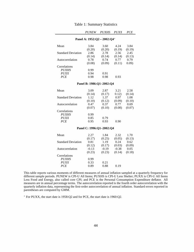
Table 1: Summary Statistics

PUNEW PUXHS PUXX PCE

Panel A: 1952:Q2 – 2002:Q4∗

Mean 3.84 3.60 4.24 3.84(0.20) (0.20) (0.19) (0.19)

Standard Deviation 2.86 2.78 2.56 2.45(0.14) (0.14) (0.14) (0.13)

Autocorrelation 0.78 0.74 0.77 0.79(0.08) (0.09) (0.11) 0.09)

CorrelationsPUXHS 0.99PUXX 0.94 0.91PCE 0.98 0.98 0.93

Panel B: 1986:Q1–2002:Q4

Mean 3.09 2.87 3.21 2.58(0.14) (0.17) 0.12) (0.14)

Standard Deviation 1.12 1.37 0.97 1.08(0.10) (0.12) (0.09) (0.10)

Autocorrelation 0.47 0.37 0.77 0.69(0.07) (0.10) (0.08) (0.07)

CorrelationsPUXHS 0.99PUXX 0.85 0.79PCE 0.95 0.93 0.90

Panel C: 1996:Q1–2002:Q4

Mean 2.27 1.84 2.32 1.70(0.17) (0.25) (0.05) (0.13)

Standard Deviation 0.81 1.19 0.24 0.62(0.12) (0.17) (0.03) (0.09)

Autocorrelation -0.13 -0.19 -0.38 0.05(0.23) (0.23) (0.14) (0.18)

CorrelationsPUXHS 0.99PUXX 0.33 0.21PCE 0.89 0.88 0.19

This table reports various moments of different measures ofannual inflation sampled at a quarterly frequency fordifferent sample periods. PUNEW is CPI-U All Items; PUXHS isCPI-U Less Shelter; PUXX is CPI-U All ItemsLess Food and Energy, also called core CPI; and PCE is the Personal Consumption Expenditure deflator. Allmeasures are in annual percentage terms. The autocorrelation reported is the fourth order autocorrelation with thequarterly inflation data, representing the first-order autocorrelation of annual inflation. Standard errors reported inparentheses are computed by GMM.

∗ For PUXX, the start date is 1958:Q2 and for PCE, the start dateis 1960:Q2.

44

Table 2: Forecasting Models

Abbreviation Specification

Time-Series Models ARMA ARMA(1,1)AR Autoregressive modelRW Random walk on quarterly inflationAORW Random walk on annual inflationRGM Univariate regime-switching model

Phillips Curve (OLS) PC1 INFL + GDPGPC2 INFL + GAP1PC3 INFL + GAP2PC4 INFL + LSHRPC5 INFL + UNEMPPC6 INFL + XLIPC7 INFL + XLI-2PC8 INFL + FACPC9 INFL + GAP1 + LSHRPC10 INFL + GAP2 + LSHR

OLS Term TS1 INFL + GDPG + RATEStructure Models TS2 INFL + GAP1 + RATE

TS3 INFL + GAP2 + RATETS4 INFL + LSHR + RATETS5 INFL + UNEMP + RATETS6 INFL + XLI + RATETS7 INFL + XLI-2 + RATETS8 INFL + FAC + RATETS9 INFL + SPDTS10 INFL + RATE + SPDTS11 INFL + GDPG + RATE + SPD

Empirical Term VAR VAR(1) on RATE, SPD, INFL, GDPGStructure Models RGMVAR Regime-switching model on RATE, SPD, INFL

No-Arbitrage Term MDL1 Three-factor affine modelStructure Models MDL2 General three-factor regime-switching model

Inflation Surveys SPF1 Survey of Professional ForecastersSPF2 Linear bias-corrected SPFSPF3 Non-linear bias-corrected SPF

LIV1 Livingston SurveyLIV2 Linear bias-corrected LivingstonLIV3 Non-linear bias-corrected Livingston

MICH1 Michigan SurveyMICH2 Linear bias-corrected MichiganMICH3 Non-linear bias-corrected Michigan

INFL refers to the inflation rate over the previous quarter; GDPG to GDP growth; GAP1 to detrended log realGDP using a quadratic trend; GAP2 to detrended log real GDP using the Hodrick-Prescott filter; LSHR to thelabor income share; UNEMP to the unemployment rate; XLI to the Stock-Watson Experimental Leading Index;XLI-2 to the Stock-Watson Experimental Leading Index-2; FAC to an aggregate composite real activity factorconstructed by Bernanke, Boivin and Eliasz (2005); RATE to the one-quarter yield; and SPD to the differencebetween the 20-quarter and the one-quarter yield.

45

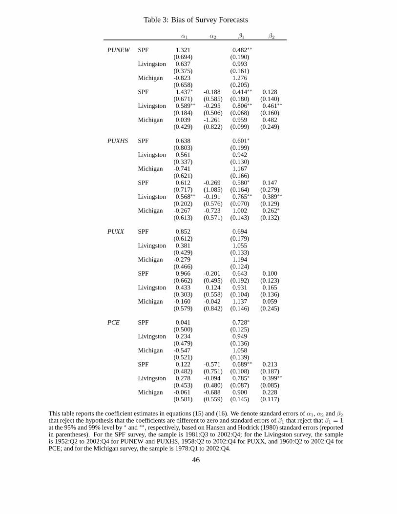
Table 3: Bias of Survey Forecasts

α1 α2 β1 β2

PUNEW SPF 1.321 0.482∗∗

(0.694) (0.190)Livingston 0.637 0.993

(0.375) (0.161)Michigan -0.823 1.276

(0.658) (0.205)SPF 1.437∗ -0.188 0.414∗∗ 0.128

(0.671) (0.585) (0.180) (0.140)Livingston 0.589∗∗ -0.295 0.806∗∗ 0.461∗∗

(0.184) (0.506) (0.068) (0.160)Michigan 0.039 -1.261 0.959 0.482

(0.429) (0.822) (0.099) (0.249)

PUXHS SPF 0.638 0.601∗

(0.803) (0.199)Livingston 0.561 0.942

(0.337) (0.130)Michigan -0.741 1.167

(0.621) (0.166)SPF 0.612 -0.269 0.580∗ 0.147

(0.717) (1.085) (0.164) (0.279)Livingston 0.568∗∗ -0.191 0.765∗∗ 0.389∗∗

(0.202) (0.576) (0.070) (0.129)Michigan -0.267 -0.723 1.002 0.262∗

(0.613) (0.571) (0.143) (0.132)

PUXX SPF 0.852 0.694(0.612) (0.179)

Livingston 0.381 1.055(0.429) (0.133)

Michigan -0.279 1.194(0.466) (0.124)

SPF 0.966 -0.201 0.643 0.100(0.662) (0.495) (0.192) (0.123)

Livingston 0.433 0.124 0.931 0.165(0.303) (0.558) (0.104) (0.136)

Michigan -0.160 -0.042 1.137 0.059(0.579) (0.842) (0.146) (0.245)

PCE SPF 0.041 0.728∗

(0.500) (0.125)Livingston 0.234 0.949

(0.479) (0.136)Michigan -0.547 1.058

(0.521) (0.139)SPF 0.122 -0.571 0.689∗∗ 0.213

(0.482) (0.751) (0.108) (0.187)Livingston 0.278 -0.094 0.785∗ 0.399∗∗

(0.453) (0.480) (0.087) (0.085)Michigan -0.061 -0.688 0.900 0.228

(0.581) (0.559) (0.145) (0.117)

This table reports the coefficient estimates in equations (15) and (16). We denote standard errors ofα1, α2 andβ2

that reject the hypothesis that the coefficients are different to zero and standard errors ofβ1 that reject thatβ1 = 1at the 95% and 99% level by∗ and∗∗, respectively, based on Hansen and Hodrick (1980) standarderrors (reportedin parentheses). For the SPF survey, the sample is 1981:Q3 to2002:Q4; for the Livingston survey, the sampleis 1952:Q2 to 2002:Q4 for PUNEW and PUXHS, 1958:Q2 to 2002:Q4for PUXX, and 1960:Q2 to 2002:Q4 forPCE; and for the Michigan survey, the sample is 1978:Q1 to 2002:Q4.

46

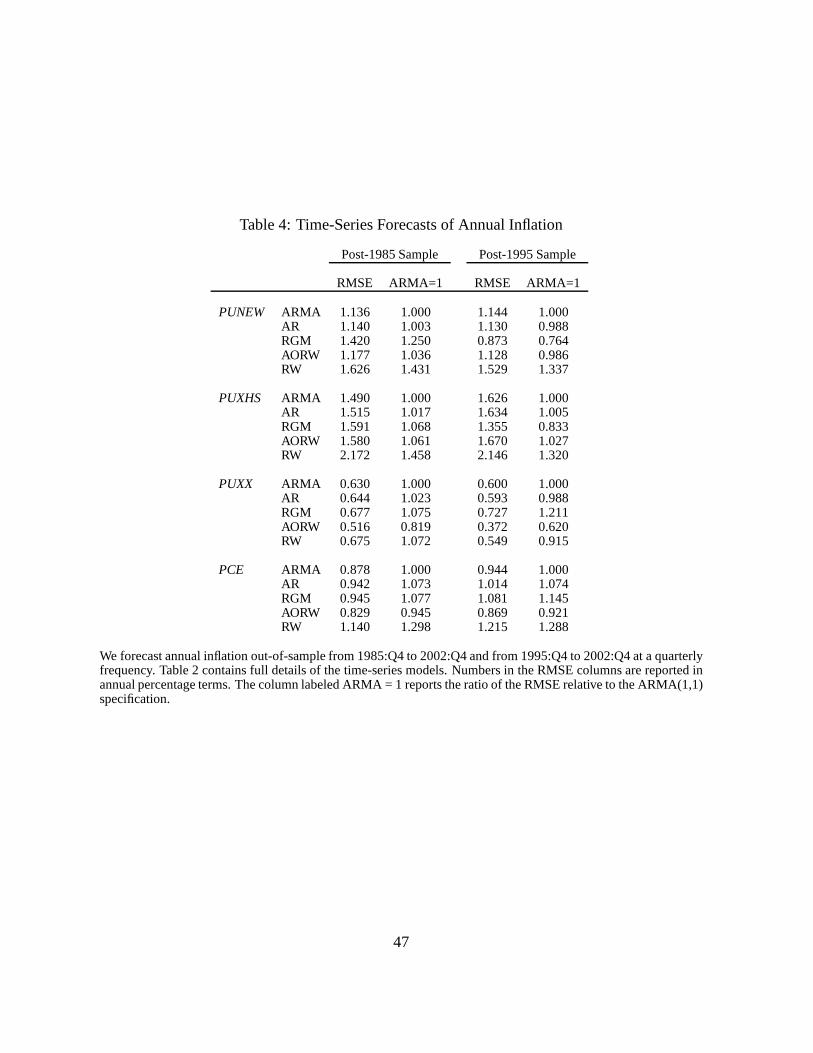
Table 4: Time-Series Forecasts of Annual Inflation

Post-1985 Sample Post-1995 Sample

RMSE ARMA=1 RMSE ARMA=1

PUNEW ARMA 1.136 1.000 1.144 1.000AR 1.140 1.003 1.130 0.988RGM 1.420 1.250 0.873 0.764AORW 1.177 1.036 1.128 0.986RW 1.626 1.431 1.529 1.337

PUXHS ARMA 1.490 1.000 1.626 1.000AR 1.515 1.017 1.634 1.005RGM 1.591 1.068 1.355 0.833AORW 1.580 1.061 1.670 1.027RW 2.172 1.458 2.146 1.320

PUXX ARMA 0.630 1.000 0.600 1.000AR 0.644 1.023 0.593 0.988RGM 0.677 1.075 0.727 1.211AORW 0.516 0.819 0.372 0.620RW 0.675 1.072 0.549 0.915

PCE ARMA 0.878 1.000 0.944 1.000AR 0.942 1.073 1.014 1.074RGM 0.945 1.077 1.081 1.145AORW 0.829 0.945 0.869 0.921RW 1.140 1.298 1.215 1.288

We forecast annual inflation out-of-sample from 1985:Q4 to 2002:Q4 and from 1995:Q4 to 2002:Q4 at a quarterlyfrequency. Table 2 contains full details of the time-seriesmodels. Numbers in the RMSE columns are reported inannual percentage terms. The column labeled ARMA = 1 reportsthe ratio of the RMSE relative to the ARMA(1,1)specification.

47

Table 5: OLS Phillips Curve Forecasts of Annual Inflation

Post-1985 Sample Post-1995 Sample

Relative HH West Relative HH WestRMSE 1 − λ SE SE RMSE 1 − λ SE SE

PUNEW PC1 0.979 0.639 0.392 0.596 0.977 0.673 0.624 0.984PC2 1.472 0.066 0.145 0.155 1.956 -0.117 0.199 0.169PC3 1.166 0.269 0.233 0.258 1.295 0.171 0.349 0.344PC4 1.078 -1.043 0.632 1.266 1.025 0.046 0.890 1.389PC5 1.032 0.354 0.288 0.372 1.115 -0.174 0.222 0.458PC6 1.103 -0.303 0.575 0.634 1.086 -0.633 0.488 1.054PC7 1.022 0.460 0.161∗∗ 0.283 1.040 0.367 0.406 0.531PC8 1.039 0.319 0.477 0.515 0.993 0.468 0.793 0.901PC9 1.576 0.006 0.119 0.144 1.994 -0.121 0.174 0.159PC10 1.264 0.146 0.205 0.235 1.426 0.119 0.246 0.287

PUXHS PC1 1.000 0.498 0.458 0.758 0.992 0.618 0.814 1.182PC2 1.328 -0.022 0.218 0.239 1.586 -0.192 0.317 0.266PC3 1.113 0.200 0.310 0.329 1.105 0.239 0.522 0.519PC4 1.096 -0.988 0.497∗ 1.064 1.029 0.008 0.745 1.229PC5 1.083 -0.080 0.299 0.491 1.076 -0.411 0.358 0.708PC6 1.131 -1.074 0.519∗ 0.822 1.061 -1.316 0.512∗∗ 1.463PC7 1.001 0.498 0.186∗∗ 0.301 1.070 0.085 0.529 0.590PC8 1.094 -0.325 0.466 0.713 1.007 0.101 1.259 1.337PC9 1.394 -0.055 0.186 0.224 1.624 -0.204 0.290 0.254PC10 1.165 0.125 0.273 0.308 1.202 0.150 0.340 0.392

PUXX PC1 0.866 1.432 0.340∗∗ 1.632 0.825 1.182 0.120∗∗ 1.384PC2 2.463 -0.120 0.072 0.100 3.257 -0.227 0.093∗ 0.119PC3 1.664 0.054 0.213 0.190 2.076 -0.063 0.275 0.226PC4 1.234 0.126 0.143 0.261 1.330 0.187 0.214 0.230PC5 1.024 0.460 0.207∗ 0.370 1.185 0.134 0.445 0.551PC6 1.005 0.479 0.477 1.053 0.916 1.009 0.277∗∗ 1.935PC7 1.074 0.381 0.277 0.426 1.089 0.293 0.500 0.731PC8 0.862 0.809 0.297∗∗ 0.751 0.767 1.127 0.275∗∗ 1.340PC9 2.485 -0.076 0.069 0.100 3.262 -0.168 0.069∗ 0.120PC10 1.873 0.079 0.136 0.153 2.562 0.038 0.150 0.151

PCE PC1 1.053 0.029 0.469 0.972 1.088 -0.240 0.434 1.119PC2 1.698 -0.136 0.141 0.178 1.997 -0.240 0.223 0.218PC3 1.274 -0.031 0.280 0.252 1.407 -0.239 0.354 0.340PC4 1.027 0.343 0.392 1.004 1.031 0.339 0.535 1.138PC5 1.125 -0.080 0.327 0.434 1.214 -0.635 0.389 0.629PC6 1.053 0.036 0.484 1.233 1.020 0.273 0.509 1.795PC7 1.033 0.436 0.175∗ 0.359 1.116 0.034 0.334 0.651PC8 1.040 0.269 0.476 0.807 1.044 0.044 1.101 2.018PC9 1.518 -0.100 0.166 0.193 1.786 -0.282 0.258 0.258PC10 1.247 0.120 0.201 0.297 1.432 -0.068 0.235 0.322

We forecast annual inflation out-of-sample over 1985:Q4 to 2002:Q4 and over 1995:Q4 to 2002:Q4 at a quarterlyfrequency. Table 2 contains full details of the Phillips Curve models. The column labelled “Relative RMSE” reportsthe ratio of the RMSE relative to the ARMA(1,1) specification. The column titled “1-λ” reports the coefficient(1 − λ) from equation (17). Standard errors computed using the Hansen-Hodrick (1980) method and the West(1996) method are reported in the columns titled “HH SE” and “West SE,” respectively. We denote standard errorsthat reject the hypothesis of(1 − λ) equal to zero at the 95% (99%) level by∗ (∗∗).

48

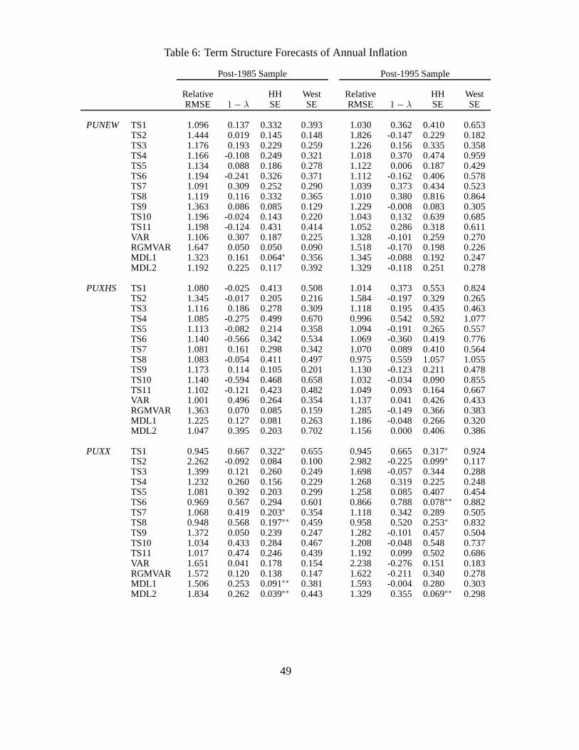
Table 6: Term Structure Forecasts of Annual Inflation

Post-1985 Sample Post-1995 Sample

Relative HH West Relative HH WestRMSE 1 − λ SE SE RMSE 1 − λ SE SE

PUNEW TS1 1.096 0.137 0.332 0.393 1.030 0.362 0.410 0.653TS2 1.444 0.019 0.145 0.148 1.826 -0.147 0.229 0.182TS3 1.176 0.193 0.229 0.259 1.226 0.156 0.335 0.358TS4 1.166 -0.108 0.249 0.321 1.018 0.370 0.474 0.959TS5 1.134 0.088 0.186 0.278 1.122 0.006 0.187 0.429TS6 1.194 -0.241 0.326 0.371 1.112 -0.162 0.406 0.578TS7 1.091 0.309 0.252 0.290 1.039 0.373 0.434 0.523TS8 1.119 0.116 0.332 0.365 1.010 0.380 0.816 0.864TS9 1.363 0.086 0.085 0.129 1.229 -0.008 0.083 0.305TS10 1.196 -0.024 0.143 0.220 1.043 0.132 0.639 0.685TS11 1.198 -0.124 0.431 0.414 1.052 0.286 0.318 0.611VAR 1.106 0.307 0.187 0.225 1.328 -0.101 0.259 0.270RGMVAR 1.647 0.050 0.050 0.090 1.518 -0.170 0.198 0.226MDL1 1.323 0.161 0.064∗ 0.356 1.345 -0.088 0.192 0.247MDL2 1.192 0.225 0.117 0.392 1.329 -0.118 0.251 0.278

PUXHS TS1 1.080 -0.025 0.413 0.508 1.014 0.373 0.553 0.824TS2 1.345 -0.017 0.205 0.216 1.584 -0.197 0.329 0.265TS3 1.116 0.186 0.278 0.309 1.118 0.195 0.435 0.463TS4 1.085 -0.275 0.499 0.670 0.996 0.542 0.592 1.077TS5 1.113 -0.082 0.214 0.358 1.094 -0.191 0.265 0.557TS6 1.140 -0.566 0.342 0.534 1.069 -0.360 0.419 0.776TS7 1.081 0.161 0.298 0.342 1.070 0.089 0.410 0.564TS8 1.083 -0.054 0.411 0.497 0.975 0.559 1.057 1.055TS9 1.173 0.114 0.105 0.201 1.130 -0.123 0.211 0.478TS10 1.140 -0.594 0.468 0.658 1.032 -0.034 0.090 0.855TS11 1.102 -0.121 0.423 0.482 1.049 0.093 0.164 0.667VAR 1.001 0.496 0.264 0.354 1.137 0.041 0.426 0.433RGMVAR 1.363 0.070 0.085 0.159 1.285 -0.149 0.366 0.383MDL1 1.225 0.127 0.081 0.263 1.186 -0.048 0.266 0.320MDL2 1.047 0.395 0.203 0.702 1.156 0.000 0.406 0.386

PUXX TS1 0.945 0.667 0.322∗ 0.655 0.945 0.665 0.317∗ 0.924TS2 2.262 -0.092 0.084 0.100 2.982 -0.225 0.099∗ 0.117TS3 1.399 0.121 0.260 0.249 1.698 -0.057 0.344 0.288TS4 1.232 0.260 0.156 0.229 1.268 0.319 0.225 0.248TS5 1.081 0.392 0.203 0.299 1.258 0.085 0.407 0.454TS6 0.969 0.567 0.294 0.601 0.866 0.788 0.078∗∗ 0.882TS7 1.068 0.419 0.203∗ 0.354 1.118 0.342 0.289 0.505TS8 0.948 0.568 0.197∗∗ 0.459 0.958 0.520 0.253∗ 0.832TS9 1.372 0.050 0.239 0.247 1.282 -0.101 0.457 0.504TS10 1.034 0.433 0.284 0.467 1.208 -0.048 0.548 0.737TS11 1.017 0.474 0.246 0.439 1.192 0.099 0.502 0.686VAR 1.651 0.041 0.178 0.154 2.238 -0.276 0.151 0.183RGMVAR 1.572 0.120 0.138 0.147 1.622 -0.211 0.340 0.278MDL1 1.506 0.253 0.091∗∗ 0.381 1.593 -0.004 0.280 0.303MDL2 1.834 0.262 0.039∗∗ 0.443 1.329 0.355 0.069∗∗ 0.298

49

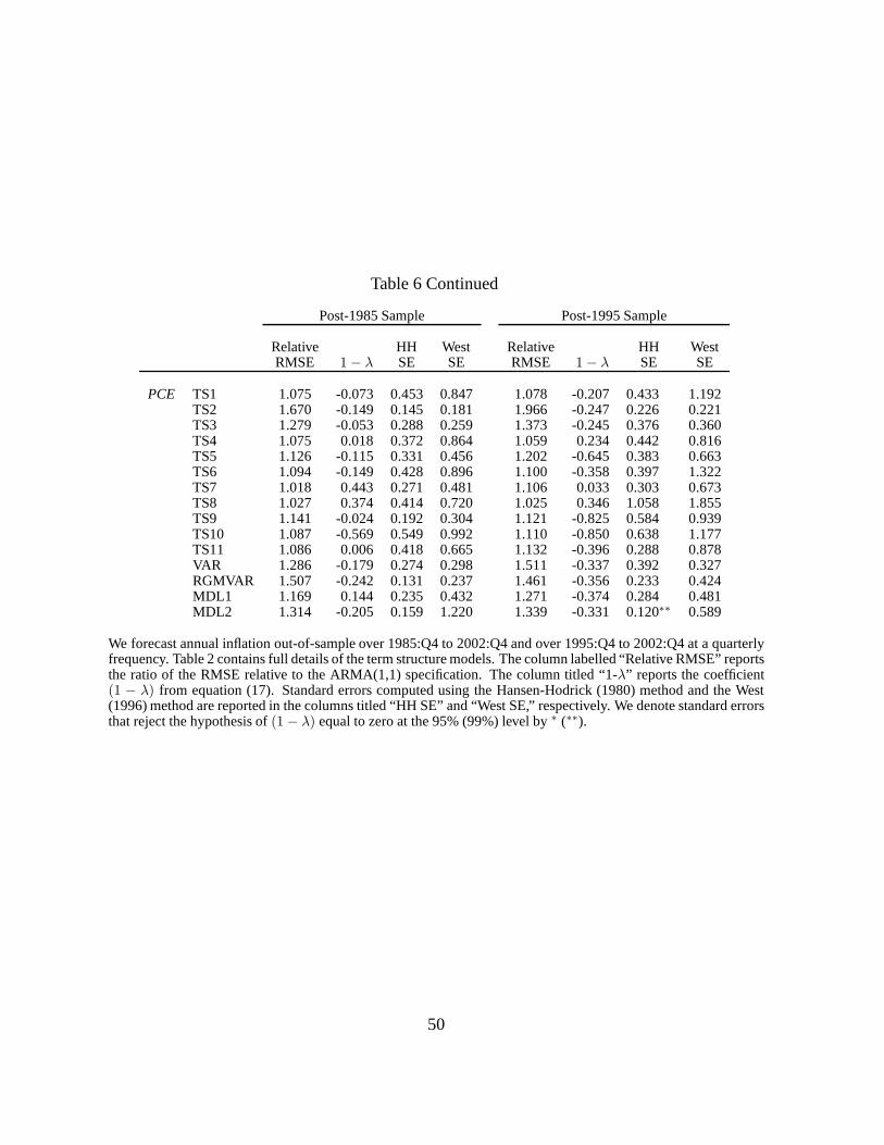
Table 6 Continued

Post-1985 Sample Post-1995 Sample

Relative HH West Relative HH WestRMSE 1 − λ SE SE RMSE 1 − λ SE SE

PCE TS1 1.075 -0.073 0.453 0.847 1.078 -0.207 0.433 1.192TS2 1.670 -0.149 0.145 0.181 1.966 -0.247 0.226 0.221TS3 1.279 -0.053 0.288 0.259 1.373 -0.245 0.376 0.360TS4 1.075 0.018 0.372 0.864 1.059 0.234 0.442 0.816TS5 1.126 -0.115 0.331 0.456 1.202 -0.645 0.383 0.663TS6 1.094 -0.149 0.428 0.896 1.100 -0.358 0.397 1.322TS7 1.018 0.443 0.271 0.481 1.106 0.033 0.303 0.673TS8 1.027 0.374 0.414 0.720 1.025 0.346 1.058 1.855TS9 1.141 -0.024 0.192 0.304 1.121 -0.825 0.584 0.939TS10 1.087 -0.569 0.549 0.992 1.110 -0.850 0.638 1.177TS11 1.086 0.006 0.418 0.665 1.132 -0.396 0.288 0.878VAR 1.286 -0.179 0.274 0.298 1.511 -0.337 0.392 0.327RGMVAR 1.507 -0.242 0.131 0.237 1.461 -0.356 0.233 0.424MDL1 1.169 0.144 0.235 0.432 1.271 -0.374 0.284 0.481MDL2 1.314 -0.205 0.159 1.220 1.339 -0.331 0.120∗∗ 0.589

We forecast annual inflation out-of-sample over 1985:Q4 to 2002:Q4 and over 1995:Q4 to 2002:Q4 at a quarterlyfrequency. Table 2 contains full details of the term structure models. The column labelled “Relative RMSE” reportsthe ratio of the RMSE relative to the ARMA(1,1) specification. The column titled “1-λ” reports the coefficient(1 − λ) from equation (17). Standard errors computed using the Hansen-Hodrick (1980) method and the West(1996) method are reported in the columns titled “HH SE” and “West SE,” respectively. We denote standard errorsthat reject the hypothesis of(1 − λ) equal to zero at the 95% (99%) level by∗ (∗∗).

50

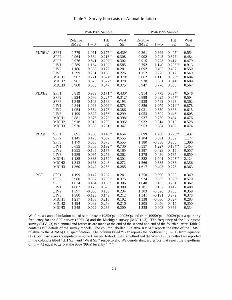
Table 7: Survey Forecasts of Annual Inflation

Post-1985 Sample Post-1995 Sample

Relative HH West Relative HH WestRMSE 1 − λ SE SE RMSE 1 − λ SE SE

PUNEW SPF1 0.779 1.051 0.177∗∗ 0.439∗ 0.861 0.869 0.407∗ 0.554SPF2 0.964 0.564 0.216∗∗ 0.308 0.902 0.745 0.377∗ 0.484SPF3 0.976 0.541 0.207∗∗ 0.302 0.915 0.728 0.414 0.479LIV1 0.789 1.164 0.102∗∗ 0.585 0.792 1.140 0.203∗∗ 0.913LIV2 1.180 0.335 0.177 0.281 1.092 0.403 0.437 0.550LIV3 1.299 0.251 0.163 0.226 1.152 0.275 0.517 0.549MICH1 0.902 0.771 0.324∗ 0.379∗ 0.862 1.113 0.520∗ 0.684MICH2 0.961 0.675 0.327∗ 0.370 0.930 0.861 0.644 0.609MICH3 0.968 0.655 0.347 0.375 0.947 0.776 0.653 0.567

PUXHS SPF1 0.819 0.939 0.171∗∗ 0.430∗ 0.914 0.773 0.394∗ 0.546SPF2 0.924 0.666 0.227∗∗ 0.312∗ 0.888 0.825 0.357∗ 0.504SPF3 1.348 0.103 0.183 0.193 0.958 0.582 0.323 0.362LIV1 0.844 1.098 0.099∗∗ 0.573 0.856 1.072 0.214∗∗ 0.878LIV2 1.054 0.554 0.176∗∗ 0.386 1.031 0.550 0.366 0.615LIV3 1.199 0.327 0.156∗ 0.299 1.053 0.502 0.443 0.605MICH1 0.881 0.876 0.273∗∗ 0.398∗ 0.937 0.750 0.434 0.476MICH2 0.918 0.815 0.290∗∗ 0.395∗ 0.932 0.814 0.515 0.528MICH3 0.970 0.608 0.251∗ 0.347 0.953 0.684 0.492 0.474

PUXX SPF1 0.691 0.968 0.140∗∗ 0.654 0.699 1.260 0.225∗∗ 1.437SPF2 1.145 0.125 0.362 0.555 1.104 0.091 0.852 1.177SPF3 1.179 0.035 0.373 0.555 1.180 -0.358 0.956 1.390LIV1 0.655 0.803 0.192∗∗ 0.730 0.557 1.227 0.134∗∗ 1.453LIV2 1.355 -0.185 0.177 0.185 1.387 -0.423 0.415 0.557LIV3 1.289 -0.095 0.259 0.262 1.278 -0.496 0.735 0.850MICH1 1.185 0.383 0.159∗ 0.301 0.822 1.041 0.208∗∗ 2.124MICH2 1.343 -0.153 0.248 0.272 1.566 -0.385 0.286 0.356MICH3 1.360 -0.242 0.253 0.285 1.617 -0.493 0.273 0.363

PCE SPF1 1.199 0.147 0.267 0.241 1.250 0.090 0.395 0.349SPF2 0.980 0.537 0.206∗∗ 0.375 0.924 0.655 0.325∗ 0.570SPF3 1.034 0.454 0.180∗ 0.306 1.040 0.453 0.234 0.362LIV1 1.082 0.175 0.325 0.300 1.101 0.132 0.412 0.400LIV2 1.397 -0.050 0.189 0.234 1.303 -0.026 0.265 0.358LIV3 1.380 -0.123 0.149 0.212 1.341 -0.191 0.272 0.375MICH1 1.217 0.108 0.216 0.192 1.338 -0.030 0.327 0.283MICH2 1.194 0.039 0.253 0.216 1.205 0.056 0.415 0.350MICH3 1.248 -0.022 0.239 0.200 1.255 -0.003 0.399 0.334

We forecast annual inflation out-of-sample over 1985:Q4 to 2002:Q4 and from 1995:Q4 to 2002:Q4 at a quarterlyfrequency for the SPF survey (SPF1-3) and the Michigan survey (MICH1-3). The frequency of the Livingstonsurvey (LIV1-3) is biannual and forecasts are made at the endof the second and end of the fourth quarter. Table 2contains full details of the survey models. The column labelled “Relative RMSE” reports the ratio of the RMSErelative to the ARMA(1,1) specification. The column titled “1-λ” reports the coefficient(1 − λ) from equation(17). Standard errors computed using the Hansen-Hodrick (1980) method and the West (1996) method are reportedin the columns titled “HH SE” and “West SE,” respectively. Wedenote standard errors that reject the hypothesisof (1 − λ) equal to zero at the 95% (99%) level by∗ (∗∗).

51

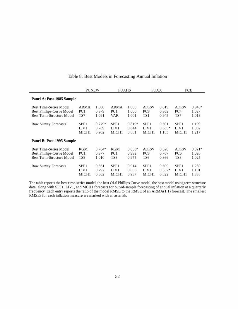
Table 8: Best Models in Forecasting Annual Inflation

PUNEW PUXHS PUXX PCE

Panel A: Post-1985 Sample

Best Time-Series Model ARMA 1.000 ARMA 1.000 AORW 0.819 AORW0.945*Best Phillips-Curve Model PC1 0.979 PC1 1.000 PC8 0.862 PC4 1.027Best Term-Structure Model TS7 1.091 VAR 1.001 TS1 0.945 TS7 1.018

Raw Survey Forecasts SPF1 0.779* SPF1 0.819* SPF1 0.691 SPF11.199LIV1 0.789 LIV1 0.844 LIV1 0.655* LIV1 1.082MICH1 0.902 MICH1 0.881 MICH1 1.185 MICH1 1.217

Panel B: Post-1995 Sample

Best Time-Series Model RGM 0.764* RGM 0.833* AORW 0.620 AORW0.921*Best Phillips-Curve Model PC1 0.977 PC1 0.992 PC8 0.767 PC6 1.020Best Term-Structure Model TS8 1.010 TS8 0.975 TS6 0.866 TS8 1.025

Raw Survey Forecasts SPF1 0.861 SPF1 0.914 SPF1 0.699 SPF1 1.250LIV1 0.792 LIV1 0.856 LIV1 0.557* LIV1 1.101MICH1 0.862 MICH1 0.937 MICH1 0.822 MICH1 1.338

The table reports the best time-series model, the best OLS Phillips Curve model, the best model using term structuredata, along with SPF1, LIV1, and MCH1 forecasts for out-of-sample forecasting of annual inflation at a quarterlyfrequency. Each entry reports the ratio of the model RMSE to the RMSE of an ARMA(1,1) forecast. The smallestRMSEs for each inflation measure are marked with an asterisk.

52

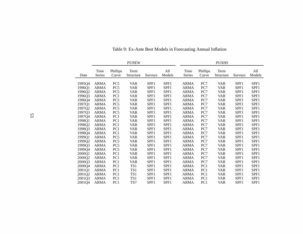
Table 9: Ex-Ante Best Models in Forecasting Annual Inflation

PUNEW PUXHS

Time Phillips Term All Time Phillips Term AllDate Series Curve Structure Surveys Models Series Curve Structure Surveys Models

1995Q4 ARMA PC5 VAR SPF1 SPF1 ARMA PC7 VAR SPF1 SPF11996Q1 ARMA PC5 VAR SPF1 SPF1 ARMA PC7 VAR SPF1 SPF11996Q2 ARMA PC5 VAR SPF1 SPF1 ARMA PC7 VAR SPF1 SPF11996Q3 ARMA PC1 VAR SPF1 SPF1 ARMA PC7 VAR SPF1 SPF11996Q4 ARMA PC5 VAR SPF1 SPF1 ARMA PC7 VAR SPF1 SPF11997Q1 ARMA PC5 VAR SPF1 SPF1 ARMA PC7 VAR SPF1 SPF11997Q2 ARMA PC5 VAR SPF1 SPF1 ARMA PC7 VAR SPF1 SPF11997Q3 ARMA PC5 VAR SPF1 SPF1 ARMA PC7 VAR SPF1 SPF11997Q4 ARMA PC1 VAR SPF1 SPF1 ARMA PC7 VAR SPF1 SPF11998Q1 ARMA PC1 VAR SPF1 SPF1 ARMA PC7 VAR SPF1 SPF11998Q2 ARMA PC1 VAR SPF1 SPF1 ARMA PC7 VAR SPF1 SPF11998Q3 ARMA PC1 VAR SPF1 SPF1 ARMA PC7 VAR SPF1 SPF11998Q4 ARMA PC1 VAR SPF1 SPF1 ARMA PC7 VAR SPF1 SPF11999Q1 ARMA PC5 VAR SPF1 SPF1 ARMA PC7 VAR SPF1 SPF11999Q2 ARMA PC5 VAR SPF1 SPF1 ARMA PC7 VAR SPF1 SPF11999Q3 ARMA PC5 VAR SPF1 SPF1 ARMA PC7 VAR SPF1 SPF11999Q4 ARMA PC5 VAR SPF1 SPF1 ARMA PC7 VAR SPF1 SPF12000Q1 ARMA PC1 VAR SPF1 SPF1 ARMA PC7 VAR SPF1 SPF12000Q2 ARMA PC1 VAR SPF1 SPF1 ARMA PC7 VAR SPF1 SPF12000Q3 ARMA PC1 VAR SPF1 SPF1 ARMA PC7 VAR SPF1 SPF12000Q4 ARMA PC1 TS1 SPF1 SPF1 ARMA PC1 VAR SPF1 SPF12001Q1 ARMA PC1 TS1 SPF1 SPF1 ARMA PC1 VAR SPF1 SPF12001Q2 ARMA PC1 TS1 SPF1 SPF1 ARMA PC1 VAR SPF1 SPF12001Q3 ARMA PC1 TS1 SPF1 SPF1 ARMA PC1 VAR SPF1 SPF12001Q4 ARMA PC1 TS7 SPF1 SPF1 ARMA PC1 VAR SPF1 SPF1

53

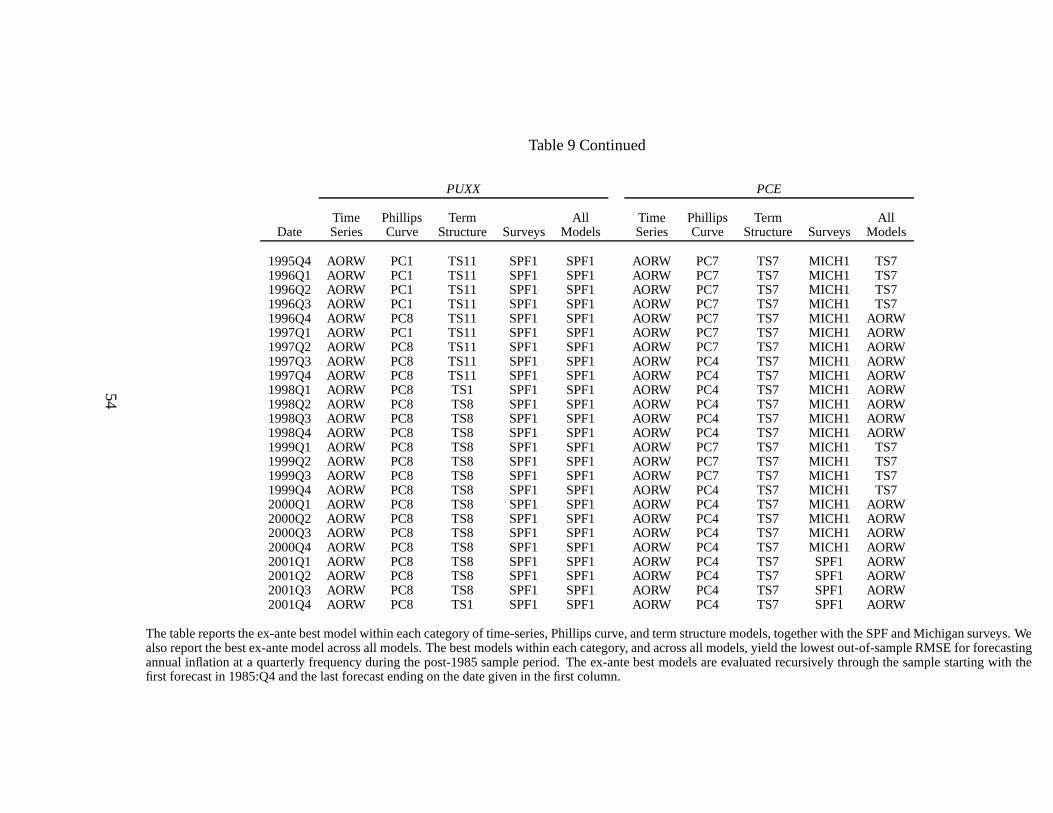
Table 9 Continued

PUXX PCE

Time Phillips Term All Time Phillips Term AllDate Series Curve Structure Surveys Models Series Curve Structure Surveys Models

1995Q4 AORW PC1 TS11 SPF1 SPF1 AORW PC7 TS7 MICH1 TS71996Q1 AORW PC1 TS11 SPF1 SPF1 AORW PC7 TS7 MICH1 TS71996Q2 AORW PC1 TS11 SPF1 SPF1 AORW PC7 TS7 MICH1 TS71996Q3 AORW PC1 TS11 SPF1 SPF1 AORW PC7 TS7 MICH1 TS71996Q4 AORW PC8 TS11 SPF1 SPF1 AORW PC7 TS7 MICH1 AORW1997Q1 AORW PC1 TS11 SPF1 SPF1 AORW PC7 TS7 MICH1 AORW1997Q2 AORW PC8 TS11 SPF1 SPF1 AORW PC7 TS7 MICH1 AORW1997Q3 AORW PC8 TS11 SPF1 SPF1 AORW PC4 TS7 MICH1 AORW1997Q4 AORW PC8 TS11 SPF1 SPF1 AORW PC4 TS7 MICH1 AORW1998Q1 AORW PC8 TS1 SPF1 SPF1 AORW PC4 TS7 MICH1 AORW1998Q2 AORW PC8 TS8 SPF1 SPF1 AORW PC4 TS7 MICH1 AORW1998Q3 AORW PC8 TS8 SPF1 SPF1 AORW PC4 TS7 MICH1 AORW1998Q4 AORW PC8 TS8 SPF1 SPF1 AORW PC4 TS7 MICH1 AORW1999Q1 AORW PC8 TS8 SPF1 SPF1 AORW PC7 TS7 MICH1 TS71999Q2 AORW PC8 TS8 SPF1 SPF1 AORW PC7 TS7 MICH1 TS71999Q3 AORW PC8 TS8 SPF1 SPF1 AORW PC7 TS7 MICH1 TS71999Q4 AORW PC8 TS8 SPF1 SPF1 AORW PC4 TS7 MICH1 TS72000Q1 AORW PC8 TS8 SPF1 SPF1 AORW PC4 TS7 MICH1 AORW2000Q2 AORW PC8 TS8 SPF1 SPF1 AORW PC4 TS7 MICH1 AORW2000Q3 AORW PC8 TS8 SPF1 SPF1 AORW PC4 TS7 MICH1 AORW2000Q4 AORW PC8 TS8 SPF1 SPF1 AORW PC4 TS7 MICH1 AORW2001Q1 AORW PC8 TS8 SPF1 SPF1 AORW PC4 TS7 SPF1 AORW2001Q2 AORW PC8 TS8 SPF1 SPF1 AORW PC4 TS7 SPF1 AORW2001Q3 AORW PC8 TS8 SPF1 SPF1 AORW PC4 TS7 SPF1 AORW2001Q4 AORW PC8 TS1 SPF1 SPF1 AORW PC4 TS7 SPF1 AORW

The table reports the ex-ante best model within each category of time-series, Phillips curve, and term structure models, together with the SPF and Michigan surveys. Wealso report the best ex-ante model across all models. The best models within each category, and across all models, yield the lowest out-of-sample RMSE for forecastingannual inflation at a quarterly frequency during the post-1985 sample period. The ex-ante best models are evaluated recursively through the sample starting with thefirst forecast in 1985:Q4 and the last forecast ending on the date given in the first column.

54

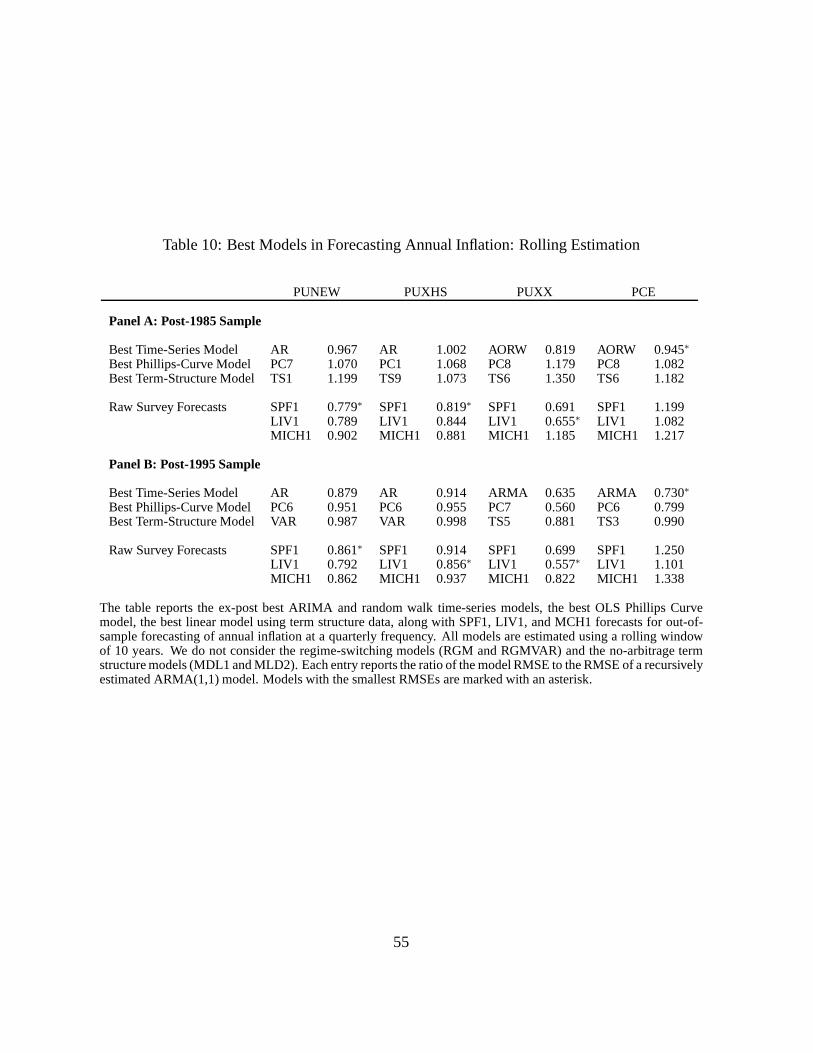
Table 10: Best Models in Forecasting Annual Inflation: Rolling Estimation

PUNEW PUXHS PUXX PCE

Panel A: Post-1985 Sample

Best Time-Series Model AR 0.967 AR 1.002 AORW 0.819 AORW 0.945∗

Best Phillips-Curve Model PC7 1.070 PC1 1.068 PC8 1.179 PC8 1.082Best Term-Structure Model TS1 1.199 TS9 1.073 TS6 1.350 TS6 1.182

Raw Survey Forecasts SPF1 0.779∗ SPF1 0.819∗ SPF1 0.691 SPF1 1.199LIV1 0.789 LIV1 0.844 LIV1 0.655∗ LIV1 1.082MICH1 0.902 MICH1 0.881 MICH1 1.185 MICH1 1.217

Panel B: Post-1995 Sample

Best Time-Series Model AR 0.879 AR 0.914 ARMA 0.635 ARMA 0.730∗

Best Phillips-Curve Model PC6 0.951 PC6 0.955 PC7 0.560 PC6 0.799Best Term-Structure Model VAR 0.987 VAR 0.998 TS5 0.881 TS3 0.990

Raw Survey Forecasts SPF1 0.861∗ SPF1 0.914 SPF1 0.699 SPF1 1.250LIV1 0.792 LIV1 0.856∗ LIV1 0.557∗ LIV1 1.101MICH1 0.862 MICH1 0.937 MICH1 0.822 MICH1 1.338

The table reports the ex-post best ARIMA and random walk time-series models, the best OLS Phillips Curvemodel, the best linear model using term structure data, along with SPF1, LIV1, and MCH1 forecasts for out-of-sample forecasting of annual inflation at a quarterly frequency. All models are estimated using a rolling windowof 10 years. We do not consider the regime-switching models (RGM and RGMVAR) and the no-arbitrage termstructure models (MDL1 and MLD2). Each entry reports the ratio of the model RMSE to the RMSE of a recursivelyestimated ARMA(1,1) model. Models with the smallest RMSEs are marked with an asterisk.

55

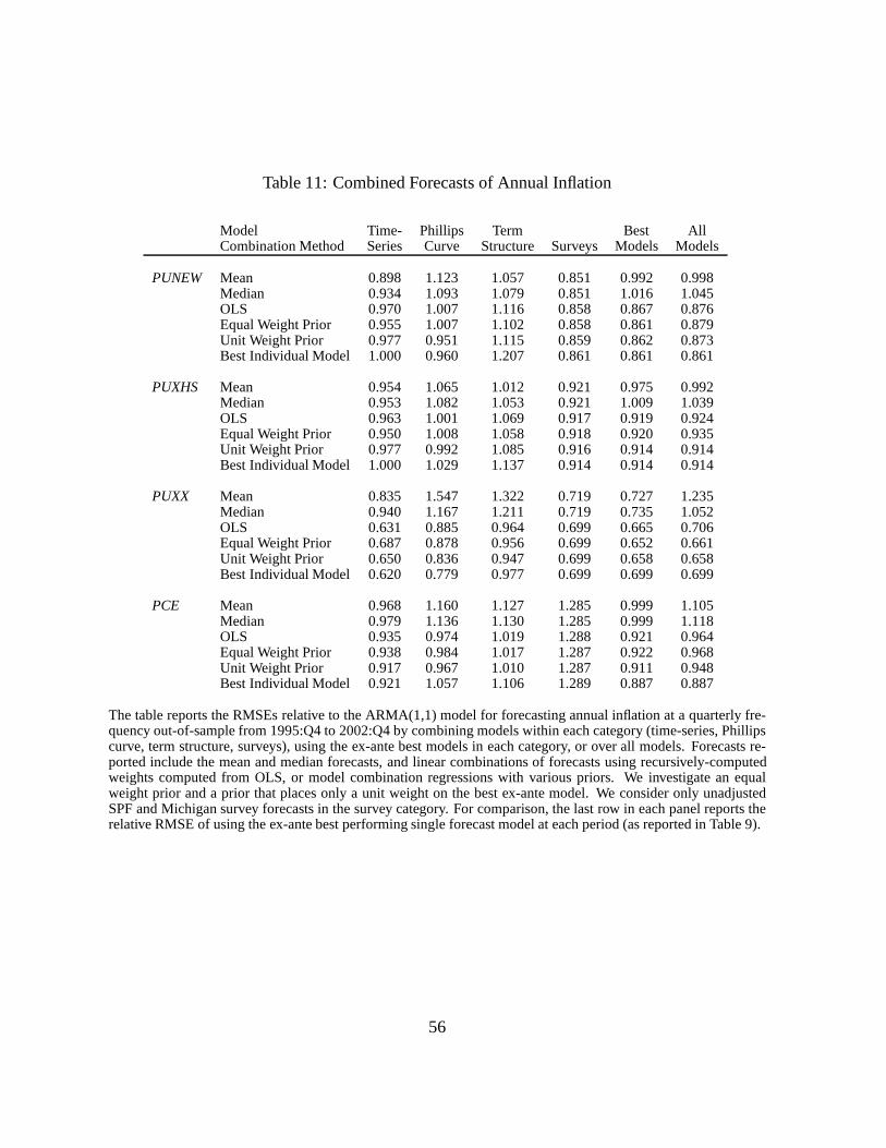
Table 11: Combined Forecasts of Annual Inflation

Model Time- Phillips Term Best AllCombination Method Series Curve Structure Surveys Models Models

PUNEW Mean 0.898 1.123 1.057 0.851 0.992 0.998Median 0.934 1.093 1.079 0.851 1.016 1.045OLS 0.970 1.007 1.116 0.858 0.867 0.876Equal Weight Prior 0.955 1.007 1.102 0.858 0.861 0.879Unit Weight Prior 0.977 0.951 1.115 0.859 0.862 0.873Best Individual Model 1.000 0.960 1.207 0.861 0.861 0.861

PUXHS Mean 0.954 1.065 1.012 0.921 0.975 0.992Median 0.953 1.082 1.053 0.921 1.009 1.039OLS 0.963 1.001 1.069 0.917 0.919 0.924Equal Weight Prior 0.950 1.008 1.058 0.918 0.920 0.935Unit Weight Prior 0.977 0.992 1.085 0.916 0.914 0.914Best Individual Model 1.000 1.029 1.137 0.914 0.914 0.914

PUXX Mean 0.835 1.547 1.322 0.719 0.727 1.235Median 0.940 1.167 1.211 0.719 0.735 1.052OLS 0.631 0.885 0.964 0.699 0.665 0.706Equal Weight Prior 0.687 0.878 0.956 0.699 0.652 0.661Unit Weight Prior 0.650 0.836 0.947 0.699 0.658 0.658Best Individual Model 0.620 0.779 0.977 0.699 0.699 0.699

PCE Mean 0.968 1.160 1.127 1.285 0.999 1.105Median 0.979 1.136 1.130 1.285 0.999 1.118OLS 0.935 0.974 1.019 1.288 0.921 0.964Equal Weight Prior 0.938 0.984 1.017 1.287 0.922 0.968Unit Weight Prior 0.917 0.967 1.010 1.287 0.911 0.948Best Individual Model 0.921 1.057 1.106 1.289 0.887 0.887

The table reports the RMSEs relative to the ARMA(1,1) model for forecasting annual inflation at a quarterly fre-quency out-of-sample from 1995:Q4 to 2002:Q4 by combining models within each category (time-series, Phillipscurve, term structure, surveys), using the ex-ante best models in each category, or over all models. Forecasts re-ported include the mean and median forecasts, and linear combinations of forecasts using recursively-computedweights computed from OLS, or model combination regressions with various priors. We investigate an equalweight prior and a prior that places only a unit weight on the best ex-ante model. We consider only unadjustedSPF and Michigan survey forecasts in the survey category. For comparison, the last row in each panel reports therelative RMSE of using the ex-ante best performing single forecast model at each period (as reported in Table 9).

56

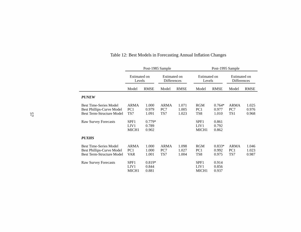
Table 12: Best Models in Forecasting Annual Inflation Changes

Post-1985 Sample Post-1995 Sample

Estimated on Estimated on Estimated on Estimated onLevels Differences Levels Differences

Model RMSE Model RMSE Model RMSE Model RMSE

PUNEW

Best Time-Series Model ARMA 1.000 ARMA 1.071 RGM 0.764* ARMA 1.025Best Phillips-Curve Model PC1 0.979 PC7 1.005 PC1 0.977 PC7 0.976Best Term-Structure Model TS7 1.091 TS7 1.023 TS8 1.010 TS1 0.968

Raw Survey Forecasts SPF1 0.779* SPF1 0.861LIV1 0.789 LIV1 0.792MICH1 0.902 MICH1 0.862

PUXHS

Best Time-Series Model ARMA 1.000 ARMA 1.098 RGM 0.833* ARMA 1.046Best Phillips-Curve Model PC1 1.000 PC7 1.027 PC1 0.992 PC1 1.023Best Term-Structure Model VAR 1.001 TS7 1.004 TS8 0.975 TS7 0.987

Raw Survey Forecasts SPF1 0.819* SPF1 0.914LIV1 0.844 LIV1 0.856MICH1 0.881 MICH1 0.937

57

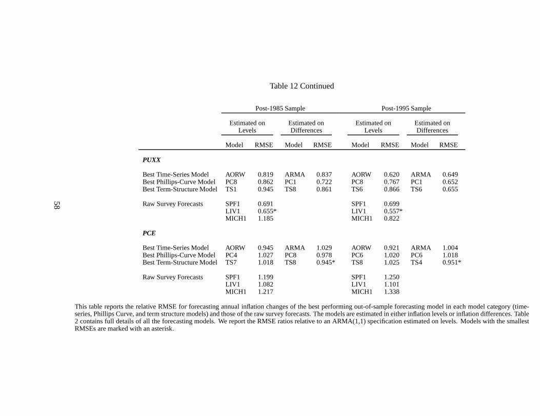
Table 12 Continued

Post-1985 Sample Post-1995 Sample

Estimated on Estimated on Estimated on Estimated onLevels Differences Levels Differences

Model RMSE Model RMSE Model RMSE Model RMSE

PUXX

Best Time-Series Model AORW 0.819 ARMA 0.837 AORW 0.620 ARMA 0.649Best Phillips-Curve Model PC8 0.862 PC1 0.722 PC8 0.767 PC1 0.652Best Term-Structure Model TS1 0.945 TS8 0.861 TS6 0.866 TS6 0.655

Raw Survey Forecasts SPF1 0.691 SPF1 0.699LIV1 0.655* LIV1 0.557*MICH1 1.185 MICH1 0.822

PCE

Best Time-Series Model AORW 0.945 ARMA 1.029 AORW 0.921 ARMA 1.004Best Phillips-Curve Model PC4 1.027 PC8 0.978 PC6 1.020 PC6 1.018Best Term-Structure Model TS7 1.018 TS8 0.945* TS8 1.025 TS4 0.951*

Raw Survey Forecasts SPF1 1.199 SPF1 1.250LIV1 1.082 LIV1 1.101MICH1 1.217 MICH1 1.338

This table reports the relative RMSE for forecasting annualinflation changes of the best performing out-of-sample forecasting model in each model category (time-series, Phillips Curve, and term structure models) and those of the raw survey forecasts. The models are estimated in either inflation levels or inflation differences. Table2 contains full details of all the forecasting models. We report the RMSE ratios relative to an ARMA(1,1) specification estimated on levels. Models with the smallestRMSEs are marked with an asterisk.

58

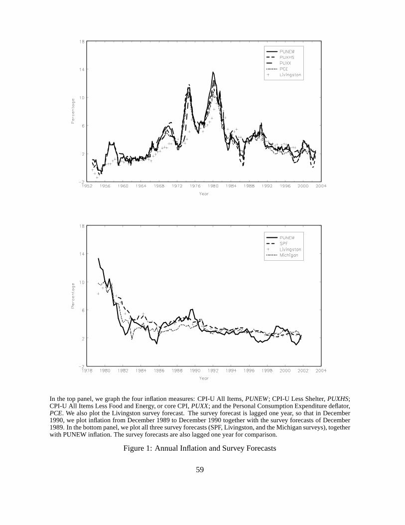
In the top panel, we graph the four inflation measures: CPI-U All Items, PUNEW; CPI-U Less Shelter,PUXHS;CPI-U All Items Less Food and Energy, or core CPI,PUXX; and the Personal Consumption Expenditure deflator,PCE. We also plot the Livingston survey forecast. The survey forecast is lagged one year, so that in December1990, we plot inflation from December 1989 to December 1990 together with the survey forecasts of December1989. In the bottom panel, we plot all three survey forecasts(SPF, Livingston, and the Michigan surveys), togetherwith PUNEW inflation. The survey forecasts are also lagged one year for comparison.

Figure 1: Annual Inflation and Survey Forecasts

59

We graph the ex-ante OLS weights on models from regression (18) over the period 1995:Q4 to 2002:Q4. Wecombine the ex-ante best model within each category (time-series, Phillips Curve, and term structure) from Table11 with the raw SPF survey. The weights are computed recursively through the sample.

Figure 2: Ex-Ante Weights on Best Models for Forecasting Annual Inflation

60

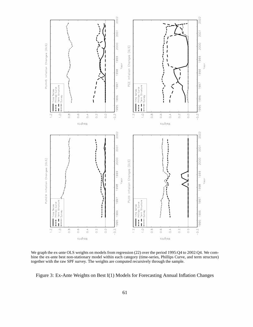
We graph the ex-ante OLS weights on models from regression (22) over the period 1995:Q4 to 2002:Q4. We com-bine the ex-ante best non-stationary model within each category (time-series, Phillips Curve, and term structure)together with the raw SPF survey. The weights are computed recursively through the sample.

Figure 3: Ex-Ante Weights on Best I(1) Models for Forecasting Annual Inflation Changes

61

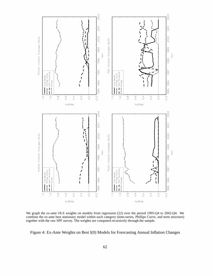
We graph the ex-ante OLS weights on models from regression (22) over the period 1995:Q4 to 2002:Q4. Wecombine the ex-ante best stationary model within each category (time-series, Phillips Curve, and term structure)together with the raw SPF survey. The weights are computed recursively through the sample.

Figure 4: Ex-Ante Weights on Best I(0) Models for Forecasting Annual Inflation Changes

62