division algebras, magic squares and supersymmetry · imperial college london division algebras,...
TRANSCRIPT

Imperial College London
Division Algebras, MagicSquares and Supersymmetry
Amel Durakovic
Submitted in partial fulfilment of the requirements for the degree of Master
of Science of Imperial College London.
September 19, 2013


Abstract
Of the four exclusive normed division algebras, only the real and
complex numbers prevail in both mathematics and physics. The non-
commutative quaternions and the nonassociative octonions have found
limited physical applications. In mathematics, division algebras unify
both classical and exceptional Lie algebras with the exceptional ones
appearing in a table known as the magic square generated by tensor
products of division algebras. This work reviews the normed division
algebras and the magic square as well as necessary preliminaries for its
construction. Space-time transformations, pure super Yang-Mills the-
ories in space-time dimensions D = 3, 4, 6, 10, dimensional reduction
and truncation of supersymmetry are also described here by the four
division algebras. Supergravity theories, seen as tensor products of
super Yang-Mills theories, are described as tensor products of division
algebras leading to the identi�cation of a magic square of supergrav-
ity theories with their U-duality groups as the magic square entries,
providing applications of all division algebras to physics and suggest-
ing division algebraic underpinnings of supersymmetry. Other curious
uses of octonions are also mentioned.
3


Contents
1 Preface 7
1.1 Acknowledgements . . . . . . . . . . . . . . . . . . . . . . . . 8
2 A pressing need 9
3 Introduction 10
4 Preliminaries 18
4.1 Nomenclature . . . . . . . . . . . . . . . . . . . . . . . . . . . 18
5 Constructing the normed division algebras 19
5.1 The quaternions . . . . . . . . . . . . . . . . . . . . . . . . . . 20
5.2 The octonions . . . . . . . . . . . . . . . . . . . . . . . . . . . 22
5.3 Split algebras . . . . . . . . . . . . . . . . . . . . . . . . . . . 26
6 The integral octonions 27
6.1 The root lattice of SO(8) . . . . . . . . . . . . . . . . . . . . . 28
6.2 The root lattice of E8 . . . . . . . . . . . . . . . . . . . . . . . 29
6.3 A �rst magic square . . . . . . . . . . . . . . . . . . . . . . . 30
7 The Jordan Algebras 32
8 Preparations 34
9 The magic square constructions 35
9.1 The Tits-Freudenthal construction . . . . . . . . . . . . . . . . 35
9.2 The Vinberg construction . . . . . . . . . . . . . . . . . . . . 37
5

9.3 The triality construction . . . . . . . . . . . . . . . . . . . . . 38
9.4 Maximal compact subalgebras . . . . . . . . . . . . . . . . . . 39
10 Division algebras in supersymmetry 40
10.1 Spinors and vectors . . . . . . . . . . . . . . . . . . . . . . . . 40
10.2 Dimensional reduction . . . . . . . . . . . . . . . . . . . . . . 44
10.2.1 Reduction to six dimensions . . . . . . . . . . . . . . . 45
10.2.2 Reduction to four dimensions . . . . . . . . . . . . . . 50
10.2.3 Reduction to three dimensions . . . . . . . . . . . . . . 52
10.2.4 Reduction of supersymmetry . . . . . . . . . . . . . . . 53
10.3 Super Yang-Mills . . . . . . . . . . . . . . . . . . . . . . . . . 54
10.3.1 Lagrangians . . . . . . . . . . . . . . . . . . . . . . . . 56
10.4 Supergravity and the magic square . . . . . . . . . . . . . . . 59
11 Summary 64
12 Outlook 65
13 References 67
6

1 Preface
This dissertation is the outcome of studies undertaken in the months June
2013 to September 2013 under Professor Michael Du� and his students at
Imperial College London. The subject matter is division algebras and their
relations to, �rst, symmetry, and, second, to supersymmetry.
Ongoing research by this group, which I have been given the opportunity
to get a �rsthand account of, seeks to establish the division algebras as the
underpinnings of theories of supersymmetry. This year, the group published
two articles on the subject where super Yang-Mills theories and supergravity
theories were treated using division algebras. [1][2] Earlier work used octo-
nions to relate black holes and quantum information theory. [3] It is the work
of this year that will be described here.
This is an introductory text that assumes no prior knowledge of the sub-
ject. It is developed beginning with division algebras, through symmetry
and �nally to supersymmetry. The structure of the text is as follows. After
the outline of the subject matter, basic de�nitions, which may be skipped
by some readers, are provided. The division algebras are thereupon de�ned
and constructed using the Cayley-Dickson procedure. The unusual division
algebras, the quaternions and the octonions, are then elaborated on, their
properties described. The split algebras, not division algebras but related,
are also introduced.
Integral division algebra elements are de�ned and used to describe root
lattices of interesting Lie algebras. The Cayley-Dickson procedure is also
applied here. Using only root lattices described by integral elements, hints
7

of a magic square are seen. Some preliminaries of the actual magic square
constructions are then introduced, the Jordan algebras and other derived
algebras. Three constructions of the magic square are described. A table
of maximal compact subalgebras corresponding to the magic square is also
provided.
Space-time transformations, spinors and vectors in the critical dimensions
D = 3, 4, 6, 10 are then formulated using division algebra elements. Dimen-
sional reduction from D = 10 to D = 6, 4, 3 is described. Super Yang-Mills
theory is further elaborated on, associating also a division algebra with the
supersymmetry of the theories. Theories of supergravity are then constructed
as tensor products of two super Yang-Mills theories. A magic square of su-
pergravity theories is found. A possible generalisation of the magic square is
discussed. The work is concluded and an outlook is provided.
1.1 Acknowledgements
Thanks to Professor Michael Du� for taking me in as a student. Special
thanks to Alexandros Anastasiou, Leo Hughes, Leron Borsten and Silvia
Nagy for invaluable help. Errors that this work may display are due to me
alone and should not in any way be associated with either Professor Michael
Du� or his students.
Thanks go to Mehmet Koca, Anthony Sudbery and Tevian Dray for tak-
ing their time by email to elaborate upon particular aspects of their work.
8

2 A pressing need
The octonions are infamous for the nonassociativity of their multiplication.
Though their multiplication is nonassociative, the state of things is not so
bad. The octonions have associative subalgebras as well as identities relating
the order of multiplication of four elements. Irrespective of whether the state
of things is ameliorated by their having associative subalgebras and identi-
ties to deal with nonassociativity, and before introducing anything concrete
at all, I feel a pressing need to dispel the aversion and defeatist attitudes
to nonassociative algebras by showing that, with or without the reader's
noticing, they are already being used. Some readers may �nd surprising that
there already are at least four nonassociative prevailing operations that enter
mathematics and physics on di�erent levels.
1. Subtraction is nonassociative since a− (b− c) = a− b+ c 6= (a− b)− c,
and division is so, too.
2. The vector product is nonassociative since (a × b) × c 6= a × (b × c).
For instance, (x× x)× y = 0 whilst x× (x× y) = x× z = −y.
3. The Lie product is nonassociative since [a, [b, c]]+[b, [c, a]]+[c, [a, b]] = 0
means that [a, [b, c]] = [[a, b], c]− [c, [a, b]] 6= [[a, b], c] in general.
Nonassociative algebras can be interesting. Sometimes, only a product of
two elements is needed and so the nonassociativity, which takes at least
three elements to be noticed, is never relevant, as is the case of the vector
product and its use in electrodynamics or motion of rigid bodies.
9

3 Introduction
There are only four normed division algebras. These are the real numbers R of
dimension one, the complex numbers C of dimension two, the quaternions H
of dimension four and the octonions O of dimension eight. The real numbers
satisfy N(ab) = N(a)N(b) where N(a) =√a2 is the norm of the real number
a. Such property holds for the complex numbers as well since N2(ab) =
(ab)(ab)∗ = aba∗b∗ which after reordering is (aa∗)(bb∗) = N2(a)N2(b) and
this also holds for the quaternions and the octonions. The division quali�er
comes from the fact that ab = 0 if and only if a = 0 or b = 0 so there is a
notion of division and a−1 = a∗/N(a) can be identi�ed as the multiplicative
(left and right) inverse of a. A normed division algebra is one for which
N(ab) = N(a)N(b) and when ab = 0 it follows that either a = 0 or b =
0. Hurwitz's celebrated theorem [4] states that there are no other normed
division algebras.
A complex number can also be regarded as a pair of real numbers with a
particular rule for multiplication of pairs. Likewise, a quaternion can be re-
garded as a pair of complex numbers and an octonion as a pair of quaternions.
This successive construction of division algebras is known as the Cayley-
Dickson procedure.
Needless to say, the real numbers and the complex numbers thrive in
mathematics as well as physics. The next division algebra after the complex
numbers, the noncommutative quaternion algebra, can be constructed by
introducing further two new imaginary elements j and k that together with
i satisfy their squaring to negative unity i2 = j2 = k2 = −1, cyclicity ij = k,
10

jk = i, ki = j and their noncommutativity where ij = −ji, ik = −ki and
jk = −kj.
A general quaternion is written q = a0 + a1i + a2j + a3k and its norm
is N(q) = a20 + a2
1 + a22 + a2
3 which is preserved by the group SO(4). An
imaginary quaternion is one spanned by imaginary elements alone such that
the quaternion has no real (or scalar) part Re(q) = a0 = 0. The three
components of the imaginary quaternion (the vector part), a1, a2 and a3,
can be identi�ed with the x, y and z components, respectively, of a vector
in Euclidean space R3. A rotation in three dimensions, fully speci�ed by
an axis of rotation p = p1i + p2j + p3k and an angle of rotation α about
this axis, is accomplished by a two-sided multiplication q′ = rqr∗ where
r = cos(α2) + sin(α
2)p and r∗ is a conjugation of r, generalising the complex
conjugation by changing the sign of all imaginary units. The scalar and vector
product as well nabla, div and curl, used in vector analysis, arise naturally
from the quaternion product. The quaternion product ab of two imaginary
quaternions a and b is ab = −a · b+a× b where the scalar product is the real
(scalar) part and the vector product is the imaginary (vector) part of the new
quaternion. Nabla was �rst introduced as ∇ = i ∂∂x
+ j ∂∂y
+ k ∂∂z
and div and
curl are the scalar and vector parts, respectively, of the quaternion product
of nabla and any imaginary quaternion. These operations were adopted in
vector analysis that superseded the quaternions.
Never mainstream, they have since only resurfaced as curiosities or failed
attempts. As a curiosity, the Pauli algebra which is isomorphic to the Cli�ord
algebra of R3 is also isomorphic to the complex quaternions C×H, and Dirac
theory is 2 × 2 over the Pauli algebra. [5][6] Cli�ord algebras generalise the
11

quaternions in higher dimensions but abandon the division algebra property.
Parallel to establishing the foundations of quantum mechanics, isospin was
an unsolved problem and it was attempted explained within the framework
of quaternionic quantum mechanics. The group SU(2) is the automorphism
group of the quaternions and arises therefore naturally for quaternions. Exact
isospin can be accounted for in quaternionic quantum mechanics but isospin
is now understood as a broken symmetry, to some extent rendering isospin a
nonproblem. [7]
The octonions are nonassociative, and since their multiplication is nonas-
sociative, they cannot be represented by matrices! The subalgebra generated
by one octonion, powers of an octonion, is associative, however. The subalge-
bra generated by any two octonions is also associative. This makes octonions
power-associative and alternative, respectively. The general octonion a can
be represented by eight real numbers, the real part a0 and seven other com-
ponents a1, . . . , a7 associated with seven imaginary elements e1, . . . , e7 such
that a = a0 + a1e1 + . . .+ a7e7, and, sometimes, a unit e0 is associated with
a0 but it is not strictly necessary. As with the quaternions, all imaginary
elements square to negative unity e2a = −1. The norm of an octonion is
N(a) = a20 + a2
1 + . . . + a27 preserved by the group SO(8). The octonion
algebra has structure constants as any other algebra. These are (excluding
e0) eaeb = Cabcec where the content of Ca
bc is best illustrated by the Fano
plane, introduced later. Including e0, the multiplication is eaeb = Γabcec, and,
if the �rst element is conjugated, e∗aeb = Γabcec. These structure constants,
Γ and Γ, can be used to construct the generators of SO(8) in its spinor and
conjugate spinor representations, and, as will be seen, generators of SO(7) in
12

its spinor and conjugate spinor representations are obtained from the above
by simply restricting ea to be an imaginary unit.
The physical applications of octonions have been scarce and scattered.
Their role in physics is unknown and they are far from mainstream. The oc-
tonions made an appearance in the Jordan program of quantum mechanics.
In establishing the foundations of quantum mechanics, alternatives to the
associative Hilbert space formulation were explored. The Jordan program
proposed to discover a new algebraic setting for quantum mechanics where
operations on observables, represented by Hermitian matrices, were also ob-
servables in principle. [8] In the Hilbert space formulation, the composition
(matrix multiplication) of observables is not an observable unless the ob-
servables commute and the adjoint operator (complex conjugate transpose)
is just the identity map on observables, hence trivial. The Hilbert space
formulation thus has super�uous operations. The only observable opera-
tions on Hermitian matrices are, in fact, powers, scalar multiplication and
addition. Elements of the Jordan algebra, the alternative algebraic setting
for quantum mechanics, are Hermitian matrices and the product is the Jor-
dan product. For two Hermitian matrices A and B, the Jordan product is
A ◦ B = 12(AB + BA) which, unlike the matrix product, is commutative.
Further imposing an axiom, the Jordan identity, implies the associativity
(unambiguity) of all powers. Unlike the matrix algebra, the Jordan algebra
is a nonassociative algebra. The complete classi�cation of Jordan algebras
contains amongst other matrix structures Hermitian quaternionic n× n ma-
trices but also 2×2 and 3×3 Hermitian octonionic matrices. The Hermitian
n× n quaternionic matrices and 2× 2 octonionic matrices are special. They
13

can be embedded in an associative algebra. The Jordan algebra of octonionic
3× 3 matrices is exceptional. It cannot be embedded in an associative alge-
bra and is hence unreachable by the associative matrix algebra Hilbert space
formulation. Deemed too small to contain quantum mechanics, unique but
only 27-dimensional, and too isolated to generalise to the in�nite-dimensional
case, in which there were later found to be no exceptional Jordan algebras,
the program was abandoned.
Octonions reappeared in another failed attempt to describe the exact
SU(3) symmetry, quark structure and con�nement. [7][9] This is no far-
fetched setup. The automorphism group of the octonions is the excep-
tional group G2 of which SU(3) is a subgroup. Other work, less known,
claims to �t the Standard Model into tensor products of division algebras
T = C⊗H⊗O. [5]
Applications of octonions and Jordan algebras to supersymmetry and
string theory came later. A one-to-one correspondence between the crit-
ical dimensions of supersymmetric theories and the division algebras was
discovered. [10] Later, simple super Yang-Mills theories in dimensions D =
3, 4, 6, 10 were related to the division algebras [11] and elaborated on [12][13].
Superstrings and super Yang-Mills theories exist in two dimensions higher
than the dimensions of the division algebras and 2-brane theories in three
dimensions higher. In D = 3, 4, 6, 10, the number of on-shell degrees of
freedom of vectors and spinors match the dimensions of R, C, H and O,
respectively, and, hence, single division algebra elements can be used to de-
scribe vectors and spinors on-shell. The isomorphisms sl(2,R) ∼= so(2, 1),
sl(2,C) ∼= so(3, 1), sl(2,H) ∼= so(5, 1) and sl(2,O) ∼= so(9, 1) relate space-
14

time transformations in D = 3, 4, 6, 10 to 2 × 2 matrices over the division
algebras. In the dimensions of the division algebras, the vector and spinor
representations are also equal.
It turns out that a vanishing quantity necessary for the supersymmetry
of both super Yang-Mills and superstring theory relies on the alternativity
of the algebra. [12] The only quantum mechanically consistent superstring
and supermembrane theories are related to the octonions, suggesting a link
between quantization of supersymmetric extended objects and nonassocia-
tivity. [7]
In mathematics, numerous works deal with octonions. There is no scarcity
of applications here. Relevant to the research presented here are the mathe-
matical applications of division algebras to constructions of classical and ex-
ceptional simple Lie algebras. Division algebras organise the classical simple
Lie algebras. [14][15] There are three in�nite families of classical Lie algebras:
so(n), su(n) and sp(n). These are constructed in an easy manner. so(n) is
just the set of n × n matrices over the real numbers x ∈ R[n] that satisfy
x∗ = −x and are traceless tr(x) = 0. su(n) is de�ned similarly but with
the n× n matrices over the complex numbers x ∈ C[n] instead. The algebra
sp(n) consists of n × n matrices over the quaternions with x∗ = −x. There
are only six exceptional simple Lie algebras. Are these then related to octo-
nions? It turns out that division algebras also organise the rare exceptional
Lie algebras but the simple construction above does not generalise to the
octonionic case. It is more subtle since matrices over the octonions do not
automatically satisfy the Jacobi identity due to their nonassociativity. [16]
As previously mentioned, the automorphism group of octonions is G2 so for
15

at least one Lie algebra, octonions are involved. [7] In fact, octonions are
implicated for the remaining cases f4, e6, e7 and e8, too. The construction
that relates the exceptional Lie algebras to octonions is exactly the magic
square construction, often displayed as a 4 × 4 table whose cells are Lie al-
gebras. The construction accepts two division algebras K1 and K2, turns K2
into a Jordan algebra H3(K2) of Hermitian 3× 3 matrices over K2 �rst, and
returns a simple Lie algebra L3(K1, H3(K2)). Details are omitted here but
tensor products K1⊗H3(K2) and subalgebra related to K1 and H3(K2) enter
the construction. [15] The magic of the magic square is that it is symmetric
even if the division algebras K1 and K2 are, a priori, not treated equally.
Later constructions of the magic square are manifestly symmetric leaving
out H3(K2) and using only K2, considering tensor products K1 ⊗ K2 but
modifying the inner workings of L3 instead. The rows and columns of the
magic square correspond to K1 and K2 that both range from R to O. The
last row (column) relates R⊗O to f4, C⊗O to e6, H⊗O to e7 and, �nally,
O⊗O to e8.
The dimensional reduction of 11-dimensional supergravity acquires non-
trivial symmetries known as U-duality groups due to toroidal compacti�ca-
tion. [17] The series of exceptional groups E6, E7 and E8 appear in reductions
of D = 11 to D = 5, 4, 3, respectively. Other slots of the Tits-Rosenfeld-
Freudenthal magic square, arise from reducingD = 9 andD = 8 supergravity
with only one slot of the magic square absent. This was the �rst instance of
exceptional groups arising as symmetries in physics without being put in by
hand, suggesting deep connections between extended theories of supergravity
and exceptional groups. [18]
16

One way to view the content (multiplets) of a theory of supergravity is as a
tensor product of the content (multiplets) of two theories of super Yang-Mills.
Given the former identi�cation of super Yang-Mills theories in the critical
dimensions with corresponding division algebras, a tensor product of division
algebra elements, each representing a super Yang-Mills �eld, can therefore
be identi�ed with a supergravity �eld. Bearing this in mind and recalling
the above construction of the magic square consisting in tensor products
of division algebras and the discovery of exceptional U-duality groups in
lower-dimensional theories of supergravity, this suggests that the Lie algebras
of the magic square construction can be identi�ed with the symmetries of
the supergravity theories obtained as a tensor products of super Yang-Mills
theories. In fact, this identi�cation was found to be true in D = 3. [2]
The dimensional reduction of vectors and spinors can also be described
by elements of division algebras. Spinors in a higher dimension reduce to
pairs of spinors in a lower dimension, reversing the Cayley-Dickson proce-
dure. For instance, a spinor in D = 10, described by an octonion, reduces to
two spinors, a pair of quaternions, in D = 6. As a result of the compacti�-
cation, the former space-time symmetries of just one object become internal
symmetries transforming two objects into one another.
Incidentally, integral elements over the four division algebras can be de-
�ned. The set of integral quaternions and integral octonions fashion the root
lattices of SO(8) and E8, respectively. [19] Other root lattices of Lie algebras
can be fashioned in a somewhat uni�ed way ultimately beginning from the
simple roots of SU(2) and the weights of its vector representation. A hint of
a magic square also appears here.
17

4 Preliminaries
De�nitions of composition algebras, division algebras, polarisation and auto-
morphisms are reviewed. The reader familiar with these concepts may skip
this section and proceed to the next where the division algebras are con-
structed using the Cayley-Dickson procedure. The split algebras will also be
constructed using the same produce modulo some signs.
4.1 Nomenclature
A composition algebra K over R with a nondegenerate quadratic form N
and an associated bilinear form 〈x, y〉 is one for which N2(xy) = N2(x)N2(y)
holds.
A division algebra is one for which xy = 0 implies that x = 0 or y = 0
which is true for composition algebras if the form is positive-de�nite. R, C, H
and O are the only positive-de�nite composition algebras and hence division
algebras.
Polarisation or linearisation obtains an bilinear form from the form N .
The inner product 〈x, y〉 = 12(N2(x+ y)−N2(x)−N2(y)).
An automorphism of an algebra is a one-to-one mapping of the algebra
onto itself with all operations of the algebra preserved. The set of automor-
phisms forms a group. Often, it is the case that automorphisms are formed
by having elements of the algebra act on itself and at the same time preserve
the algebraic structure. One example is conjugation. Such automorphisms
are called inner automorphisms. These are to be distinguished from outer
automorphisms where extrinsic elements may act on the algebra. Examples
18

of outer automorphisms are re�ections and symmetries of Dynkin diagrams
such as the triality of the SO(8) Dynkin diagram. The action of the outer
automorphism on the roots of the algebra is to permute the three elements
but permutations are not themselves elements of SO(8).
5 Constructing the normed division algebras
Although there are other composition algebras, Hurwitz's aforementioned
theorem states that R, C, H and O are the only four normed division al-
gebras. The real numbers of dimension one are real, that is to say, the
action of conjugation acts trivially on them. They are also associative and
commutative. The complex numbers of dimension two lose the property of
trivial conjugation but inherit all the other properties. The quaternions of
dimension four inherit all the properties of the complex numbers but lose
commutativity and the octonions of dimension eight, which otherwise inherit
the properties of the quaternions, lose associativity.
There is a procedure known as the Cayley-Dickson construction that gen-
erates a sequence of algebras that double in dimension and makes manifest
why the quaternions are noncommutative and the octonions nonassociative.
The �rst four algebras in this sequence are exactly the normed division al-
gebras. The reader is already familiar with the �rst step of the procedure
and the main features of its generalisation but the trivial conjugation and
commutativity of the real numbers mask the details.
A complex number can be regarded as a pair of real numbers z = (a, b)
which is most commonly written z = a+ ib with the imaginary unit i intro-
19

duced. The multiplication of two complex numbers z1 = a+ib and z2 = c+id
is just z3 = z1z2 = (a, b)(c, d) = (a + ib)(c + id) = (ac − bd) + i(ad + bc) =
(ac−bd, ad+bc). If (a, b) were a pair of complex numbers or a pair of quater-
nions the correct quaternion or octonion multiplication, respectively, would
be (a, b)(c, d) = (ac − db∗, cb + a∗d) with conjugation de�ned as (a, b)∗ =
(a∗,−b). The norm squared is zz∗ = (a, b)(a, b)∗ = (aa∗ + bb∗, 0) = aa∗ + bb∗
and the inner product is 〈(a, b), (c, d)〉 = 12((a, b)∗(c, d) + (c, d)∗(a, b)) =
(12(a∗c + c∗a + bd∗ + db∗), 0) = 1
2(a∗c + c∗a + bd∗ + db∗). Imaginary ele-
ments will greatly simplify these ghastly expressions at the cost of results
dependent on choice of basis.
A pair of octonions (a, b) is called a sedenion which is of dimension 16.
Sedenions are not division algebras. They have zero divisors. [14] They are
not alternative but the power of a sedenion is still a well-de�ned notion.
5.1 The quaternions
The above construction of the quaternions as a pair of complex numbers may
look obscure, but by introducing imaginary elements, the familiar rules of the
multiplication of imaginary units will arise. Consider two complex numbers
(x0, x1) = x0 + x1i and (x3, x2) = x3 + x2i where i is the imaginary unit
of the complex numbers that satis�es i2 = −1. A quaternion q is then a
pair of complex numbers ((x0, x1), (x3, x2)) which can also be represented by
introducing a new imaginary unit k such that q = (x0, x1)+k(x3, x2) = (x0 +
x1i)+k(x3+ix2) = x0+x1i+kix2+kx3. It can be left at this, having just two
imaginary units i and k but then the element ki would then have to be used
20

throughout which is instead named j = ki such that q = x0 +x1i+x2j+kx3.
Conjugation is represented by ((x0, x1), (x3, x2))∗ = ((x0, x1)∗,−(x3, x2)) =
x0 − x1i− x2j − x3k and the norm is ((x0, x1), (x3, x2))((x0, x1), (x3, x2))∗ =
(x0, x1)(x0, x1)∗ + (x3, x2)(x3, x2)∗ = x20 + x2
1 + x22 + x2
3.
The imaginary element k is represented as ((0, 0), (1, 0)) and its square
is k2 = ((0, 0), (1, 0))((0, 0), (1, 0)) = ((0, 0)(0, 0) − (1, 0)(1, 0)∗, (0, 0)(1, 0) +
(0, 0)∗(1, 0)) = (−(1, 0), (0, 0)) = −1. By the same procedure, it can be
seen that ij = k and ji = −k. The full multiplication table can be seen
in Figure 1. This algebra is clearly not commutative. The quaternionic
i j ki −1 k −jj −k −1 ik j −i −1
Figure 1: The multiplicationof imaginary quaternionic ele-ments.
i
j k
Figure 2: The simple cyclicmultiplication of the quater-nionic elements.
multiplication can be summarised with the Levi-Civita symbol: eaeb = −δab+
εabcec. The group that preserves the norm for real numbers is Z2. For complex
numbers it is SO(2) ∼= U(1) and given that the norm of a quaternion is
N(x) = x20 + x2
1 + x22 + x2
3, the group that preserves the norm is SO(4).
In general for division algebras, and not just for quaternions, the inner
product de�ned earlier as 〈(a, b), (c, d)〉 = 12((a, b)∗(c, d) + (c, d)∗(a, b)) =
12(a∗c + c∗a + bd∗ + db∗) can also be seen as: 〈x, y〉 = Re(xy∗) = Re(x∗y) =
12Re(xy∗ + x∗y) and collective conjugation conjugates each element but re-
orders the multiplication: (xy)∗ = y∗x∗.
Since quaternions do not commute, the commutator may be a convenient
21

quantity to consider: [x, y] = xy − yx. If any argument is conjugated, the
commutator changes sign. For quaternions [ea, eb] = 2εabcec.
Rotations are two-sided operations. The axis of rotation and the angle
of rotation is set by a vector b and α, respectively. Another vector c =
cos(α2) + sin(α
2)b is formed and the rotated vector is v′ = cvc∗. Rotation is
reversed by conjugation of the vector c.
The left Lc and right multiplication Rc∗ determined by one element c is
isomorphic to SU(2) which SO(3) is isomorphic to. By making the elements
of left and right multiplication distinct this becomes an SU(2) × SU(2) ∼=
SO(4) transformation. [20]
The elements i, j and k are not the only that square to −1. As long as it
is an imaginary quaternion and it has unit norm then it squares to −1. There
are also complex subalgebras in the quaternion algebra. They are spanned
by a real part and a unit imaginary quaternion such that C = {a + bm}
where m is an imaginary unit quaternion. In analogy to complex numbers,
emα = cos(α) + m sin(α) and any quaternion q, or octonion if m is a unit
octonion, can be written q = remα where r = |q|. [21]
The automorphism group of the quaternions, the set of transformations
that preserve the quaternionic multiplication, is SU(2).
5.2 The octonions
The octonions can now be constructed as a pair of quaternions and a simi-
lar procedure to the one in the preceding section can be followed to obtain
their multiplication rules. By introducing imaginary elements, their multi-
22

plication can be made easy, though dependent on basis. Since the procedure
is analogous to the one for quaternions, only the results will be given here.
Consider two quaternions, p and p′. The octonion k will then be a pair of
those such that k = p + e7p′, and by expressing the quaternions in terms
of their three imaginary elements, labelled for convenience, e1, e2 and e4,
p = p1 + e1p1 + e2p2 + e4p4 and p′ = p7 + p3e1 + p6e2 + p5e4, the octonion k
is written k = (p0 + p1e1 + p2e2 + p4e4) + e7(p7 + p3e1 + p6e2 + p5e4). The
elements e7e1, e7e2 and e7e4 could be used throughout or new elements could
be introduced for convenience e3 = e7e1, e6 = e7e2 and e5 = e7e4. All ele-
ments square to −1 and the full multiplication table can be seen in Figure 3.
From the multiplication, The index cycling rule (modulo 7) can be read o�,
e1 e2 e3 e4 e5 e6 e7
e1 −1 e4 e7 −e2 e6 −e5 −e3
e2 −e4 −1 e5 e1 −e3 e7 −e6
e3 −e7 −e5 −1 e6 e2 −e4 e1
e4 e2 −e1 −e6 −1 e7 e3 −e5
e5 −e6 e3 −e2 −e7 −1 e1 e4
e6 e5 −e7 e4 −e3 −e1 −1 e2
e7 e3 e6 −e1 e5 −e4 −e2 −1
Figure 3: The multiplication of octonionic imaginary units.
eiei+1 = ei+3, as well as the index doubling identity (modulo 7) that says
that eiej = ek implies e2ie2j = e2k. Noncommutativity e1e2 = e4 6= e2e1 and
nonassociativity can be seen. Nonassociativity takes three so (e2e3)e7 = −1
whilst e2(e3e7) = e2e1 = −e4 6= (e2e3)e7 = e4. However, there are also
quaternionic subalgebras in the octonion algebra for which there is associa-
tivity. There are also complex subalgebras, for which there is commutativity.
The multiplication of octonionic imaginary units can be illustrated by the
23

Fano plane, which also happens to be the smallest �nite projective plane. [14]
It has been drawn in Figure 4. The seven labelled points correspond to the
6
4 1
7
3 2 5
Figure 4: The Fano plane. Multiplication of imaginary units.
seven imaginary elements. There are seven lines each connecting three points.
They close as circles e1 → e2 → e4 → e1, e2 → e3 → e5 → e2 and so forth.
The circle on the picture also counts as a line. On the drawing, it is the
most truthful as all the other lines in fact close like the circle. There are
arrows on the lines to denote the direction of multiplication. Going against
the arrow gives the negative result. The lines (circles) are the quaternionic
subalgebras. This section began with only e1, e2, e4 and one more element
e7. It is now easy to see that this is enough. The other elements can be
reached by multiplication of e1, e2 and e4 with e7. Conjugation changes the
sign of all the imaginary elements and the norm is the sum of the squared
components. The group that preserves the octonionic norm is SO(8). The
transformations that preserve the octonionic multiplication is isomorphic to
the exceptional group G2. SU(3) is the maximal subgroup of G2. It is the
24
automorphism group involving six octonionic units. [9]
The octonions are power-associative which means that the subalgebra of
any one element is associative. This is easily explained. Without loss of
generality, it can be assumed that the octonion sits in a complex subalgebra.
The octonions are alternative which means that the subalgebra formed by
any two elements is associative. Since there are only two octonions, they
can be assumed without loss of generality to sit in a quaternionic subalgebra
which explains alternativity. Furthermore, the octonions satisfy the Moufang
laws involving four octonions which say that (xyx)z = x[y(xz)], z(xyx) =
[(zx)y]x, and (xy)(zx) = x(yz)x. [4]
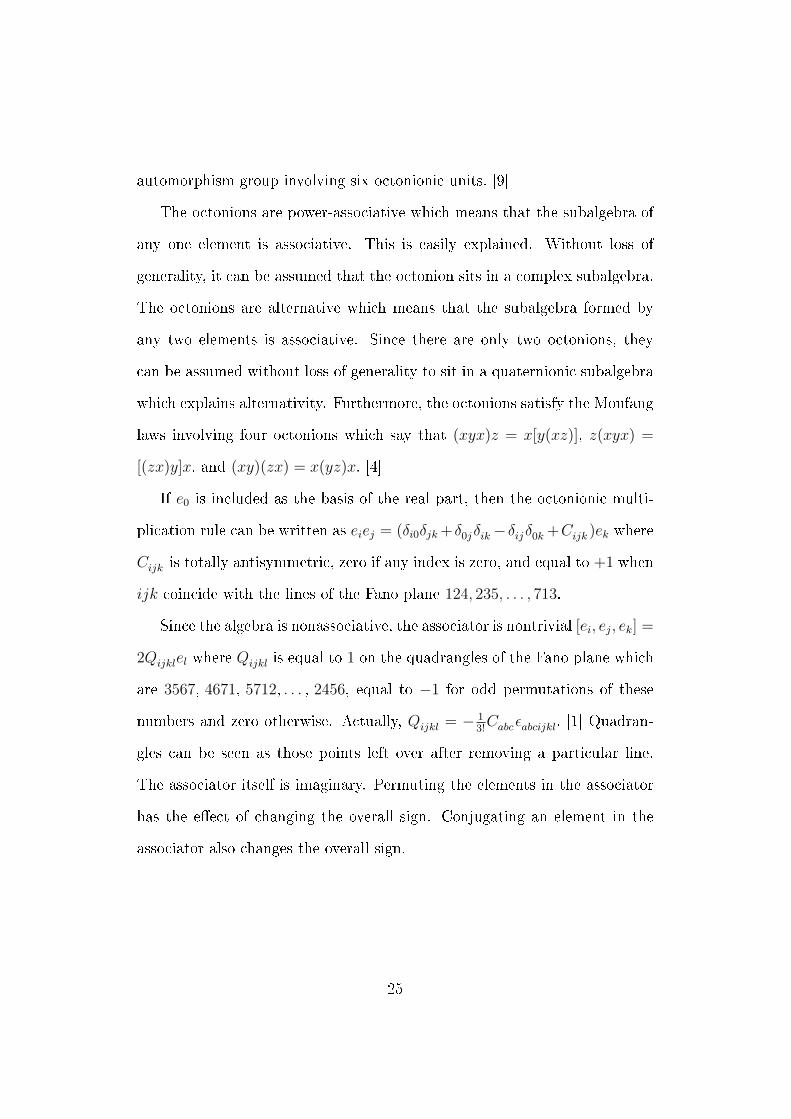
If e0 is included as the basis of the real part, then the octonionic multi-
plication rule can be written as eiej = (δi0δjk +δ0jδik−δijδ0k +Cijk )ek where
Cijk is totally antisymmetric, zero if any index is zero, and equal to +1 when
ijk coincide with the lines of the Fano plane 124, 235, . . . , 713.
Since the algebra is nonassociative, the associator is nontrivial [ei, ej, ek] =
2Qijklel where Qijkl is equal to 1 on the quadrangles of the Fano plane which
are 3567, 4671, 5712, . . . , 2456, equal to −1 for odd permutations of these
numbers and zero otherwise. Actually, Qijkl = − 13!Cabcεabcijkl. [1] Quadran-
gles can be seen as those points left over after removing a particular line.
The associator itself is imaginary. Permuting the elements in the associator
has the e�ect of changing the overall sign. Conjugating an element in the
associator also changes the overall sign.
25

5.3 Split algebras
The Cayley-Dickson procedure can be used to construct other algebras known
as the split algebras C, H and O which are also composition algebras. It
involves changing signs in the Cayley-Dickson construction. [22] The �rst step
to get other 2-dimensional hypercomplex numbers (algebras) is to introduce
a real number µ in the Cayley-Dickson procedure and let multiplication in
the new algebra be (a, b)(c, d) = (ac− µd∗b, da− bc∗). As before, an element
(a, b) in the new algebra may be represented as z = a + eb and it is readily
found that e2 = −µ. This follows from starting with e = (0, 1) and so
e2 = (0, 1)(0, 1) = (−µ, 0) = −µ. The squared norm of a N(z) = zz∗ =
z∗z = a2 + µb2 and so three algebras distinct algebras can arise:
1. the complex numbers, C when µ = 1 with norm N(z) = a2 + b2,
2. the split complex numbers C(−1) with µ = −1 and norm N(z) =
a2 − b2,
3. the dual numbers C(0) with µ = 0 and norm N(z) = a2.
Of these, only the complex numbers form a division algebra.
Continuing by now considering a pair of complex numbers z1 and z2 such
that z = (z1, z2) represented as z1 + ez2 where, as before, e2 = −µ. Again,
there are three nonisomorphic algebras:
1. the quaternions H = H(1, 1) with µ = 1 norm N(x) = x20 +x2
1 +x22 +x2
3,
2. the split quaternions H = H(1,−1) with µ = −1, norm N(x) = x20 +
x21 − x2
2 − x23 and imaginary elements i2 = −1 but k2 = j2 = 1,
26

3. the semiquaternions H(1, 0) with µ = 0, norm N(x) = x20 + x2
1 and
imaginary elements i2 = −1 and j2 = k2 = 0.
Starting with a pair of quaternions, analogous considerations generate the
octonions O(1, 1, 1) (µ = 1), the split octonions O = O(1, 1,−1) and the
semioctonions O(1, 1, 0). The split octonions have three imaginary elements
that square to −1 and four that square to 1. Their norm is N(x) = x20 +x2
1 +
x22 + x2
3 − x24 − x2
5 − x26 − x2
7.
In general, H(µ1, µ2) and O(µ1, µ2, µ3) could also have been considered
and the forms N(x) = x20 + µ1x
21 + µ2x
22 + µ1µ2x
33 and N(x) = x2
0 + µ1x21 +
µ2x22 + µ3x
24 + µ1µ3x
25 + µ2µ3x
26 + µ1µ2µ3x
27 would have been found.
Incidentally, there is a reason for their being called split algebras. [15]
The equation de�ning the square of some of the imaginary elements can be
split into two factors: i2 = 1 ⇒ i2 − 1 = 0 ⇒ (i + 1)(i − 1) = 0. It is here
easy to see that this is not a division algebra: There are zero divisors since
two nonzero elements i + 1 and i − 1, not zero themselves, multiply to give
zero.
6 The integral octonions
Any element x of a division algebra A satis�es the rank equation: x2 − (x+
x∗)x+ xx∗ = 0. [19] The factor in the second term (x+ x∗) is twice the real
part and the last term is the norm squared xx∗. If the elements of a set A
obey the rank equation with integer norm, if the double scalar part is integer,
and if
1. A is closed under multiplication and subtraction,
27

2. A contains the identity,
3. A is not a subset of a larger set that also satis�es 1 and 2,
then the elements of A are called integral elements. There is a set of 240
(integral) octonions that satis�es these properties. This corresponds to the
scaled root lattice of E8. There is also a set of 24 quaternions that satis�es
these properties. This is the scaled root lattice of SO(8). The roots here
are normalised to unity as opposed to the standard√
2 norm in the Cartan-
Killing classi�cation.
Weyl re�ections applied to the simple roots generate the remaining. Con-
sider two roots ra and rb. The re�ection of ra with respect to the hyperplane
that has rb as normal vector generates a new root rab = −rbr∗arb. [7]
In the following, for convenience, the permutations e4 ↔ e3, e6 ↔ e5 will
be made that di�er from the rest of the text.
6.1 The root lattice of SO(8)
The root lattice of SO(8) which has a quaternionic description is given by the
set A0 = {±1,±e1,±e2,±e3,12(±1±e1±e2±e3)}, which give the required 24
roots. The root lattice of SO(8) could have been made from SU(2)4. Tensor
products are just weights added in the Cayley-Dickson fashion. The root
lattice of SU(2) is simply {±1} and the weights of the spinor representation
are {±12}. The adjoint representation of SO(8) decomposes to SU(2)4 as
28 = (3,1,1,1)+(1,3,1,1)+(1,1,3,1)+(1,1,1,3)+(2,2,2,2) from which
one can easily obtain the roots of SO(8). The roots (3,1,1,1) are made of
the roots (adjoint) of one SU(2) and zeros (((±1, 0), 0), 0) = ±1. The roots
28

of (1,3,1,1) are (((0,±1), 0), 0) = ±e1 and so (1,1,3,1) corresponds to
(((0, 0),±1), 0) = ±e2 and (((0, 0), 0),±1) = ±e3. Finally, (2,2,2,2) =
(((±12,±1
2),±1
2),±1
2) = 1
2(±1± e1 ± e2 ± e3).
6.2 The root lattice of E8
The root lattice of E8 consists of the set ±1, ±ei, 12(±ej ± ek ± el ± em) and
12(±1±en±ep±eq) where i = 1, . . . , 7, jklm = 1246, 1257, 1345, 1367, 2356,
2347, 4567 and npq = 123, 147, 165, 245, 267, 346, 357. Incidentally, the
subset of imaginary roots form the E7 lattice. Given that there is an arbi-
trariness in the choice of imaginary elements, it is to be expected that this is
not a unique set of roots and, indeed, that is the case. There are seven other
octonionic integer sets of E8 roots. [19]
By considering the decomposition of the adjoint representation of E8 un-
der SO(8) × SO(8), this list of E8 roots can easily be generated. The de-
composition is 248 = (28,1) + (1,28) + (8v,8v) + (8s,8c) + (8c,8s). The
weights of the vector representation 8v are A1 = {12(±1 ± e1), 1
2(±e2 ± e3)}
which can be obtained by knowing that 8v = (2,2,1,1) + (1,1,2,2). The
weights of the spinor representation are 8s = (1,2,2,1) + (2,1,1,2) are
A3 = {12(±1± e3), 1
2(±e1 ± e2)} and those of the conjugate spinor represen-
tation 8c = (2,1,2,1) + (1,2,1,2) are A2 = {12(±1± e2), 1
2(±e3 ± e1)}.
Incidentally, description makes the triality of SO(8) manifest. Clearly,
permutations of the three imaginary elements e1, e2, e3 will map the repre-
sentations A1 → A2 → A3 into one another. Looking at the decomposition,
the root lattice of E8 is (A0, 0) + (0, A0) + (A1, A1) + (A3, A2) + (A2, A3).
29

The maximal compact subalgebra of E8 is SO(16) and its root lattice
consists of the set ±1, ei,12(±ej ± ek ± el ± em) and 1
2(±1 ± en ± ep ± eq)
where, now, i = 1, . . . , 7, jklm = 2356, 2347, 4567 and npq = 123, 147, 165.
Curiously, these are quaternionic subalgebras and their quadrangles!
These roots may become important for a division algebra formulation of
the supergravity Lagrangians. Root vectors already appear in Lagrangian
descriptions of supergravity theories where they are used to describe the
cosets that scalars of compacti�ed theories parameterise. [17] The N = 16,
D = 3 supergravity theory has scalars that parameterise the 128-dimensional
E8/SO(16) coset. Here, roots of both E8 and SO(16) have been given.
6.3 A �rst magic square
Interesting root lattices arise by pairing roots of the algebras SU(3), Sp(3)
and F4 with one another in the Cayley-Dickson fashion. [19]
The F4 root lattice turns out to be just the sum of the weights of the
vector, spinor and conjugate spinor representations of SO(8) and the roots
of SO(8): 48 = 24 + 8v + 8s + 8c.
The SU(3) root lattice is {±12(1 + e1),±1
2(e2− e1),±1
2(1 + e2)} generated
by the simple roots {12(1 + e1), 1
2(e2 − e1)}.
The Sp(3) roots are {±1,±e1,±e3,±(±1± e1), 12(±e1 ± e3), 1
2(±1± e3)}
generated by the simple roots {12(−1 + e1), 1
2(1− e3), e3}.
The result of matching roots amongst the Lie algebras above can be
summarised in a 4 × 4 table with the three aforementioned Lie algebras
in the margins. Short roots are matched with short roots and long roots
30

are matched with zeros. The result is shown in Figure 6. Save the empty
upper left corner, this is curiously the magic square, albeit without much
explanatory power. It is presented here as a curiosity.
In a subtle way, this construction is probably establishing the simple fact
that (K1⊗R)⊗(R⊗K2) = K1⊗K2 since the Cayley-Dickson procedure, which
was used for matching, itself is related to tensor products and the algebras
in the margin come from tensor products where one division algebra is R.
This is just a guess.
SU(3) Sp(3) F4
SU(3) SU(3)× SU(3) SU(6) E6
Sp(3) SU(6) SO(12) E7
F4 E6 E7 E8
Figure 5: The magic square. Paired roots of algebras in the margin produceroot lattices of curious groups.
Ramond notes that the Lie algebras of the magic square are interrelated,
allowing embeddings to be read o� the magic square. [20] Division algebras
also �nds applications in establishing other embeddings, not necessarily re-
lated to the magic square. [16]
It has been shown how integral elements of division algebras can be used
to describe root lattices of interesting Lie algebras. It is curious that the set
of integral octonionic elements coincides with the scaled root lattice of E8
and the set of integral quaternionic elements coincides with the scaled root
lattice of SO(8). Triality was manifest in the quaternionic description of the
SO(8) roots and weights.
31

7 The Jordan Algebras
The remnants of the failed Jordan program, the Jordan algebras, �rst in-
troduced as an alternative formulation of quantum mechanics centred on
observables, was picked up in mathematics and used in the �rst construction
of the magic square.
The Jordan algebra is a real vector space with a commutative bilinear
product x◦y = y◦x which satis�es the Jordan identity (x2◦)◦x = x2◦(y◦x).
The Jordan identity implies that Jordan algebras satisfy power-associativity.
A classi�cation of Jordan algebras exists. Simple �nite-dimensional for-
mally real1 Jordan algebras are isomorphic to one of �ve types of Jordan
algebras. [14][8] Four of the �ve types, one per division algebra, are n × n
Hermitian matrix algebras hn(A) over a division algebra A with the Jordan
(anticommutator) product a ◦ b = 12(ab + ba) where ab and ba are matrix
products. When the division algebra is O, there is a further constraint to
n ≤ 3. The case n = 3 is an exceptional Jordan algebra which means that
it cannot be realised as a subalgebra over some real associative algebra with
multiplication given by x ◦ y = 12(xy + yx). It is also the only exceptional
Jordan algebra. The (in�nitesimal) transformations that preserve the Jordan
product form the exceptional Lie algebra f4!
The last type of Jordan algebra is the spin group that lives in Rn⊕R. An
element in this space is represented by the pair (x, t) with Jordan product ◦
represented by (x, t) ◦ (x′, t′) = (tx′+ t′x,x · x′+ tt′). All spin groups can be
realised as a certain subspace of Hermitian 2n × 2n matrices.
1Sum of elements squared is zero only when the elements are individually zero: x21 +. . .+ x2n = 0⇒ x1 = . . . = xn = 0.
32

The algebras h1(O) and h2(O) are not exceptional. They are special which
means that they can be realised as a subalgebra of an associative algebra al-
gebra over the real numbers. The Jordan program sought an algebra that
could not be made from a real associative algebra where the Jordan product
◦ was implemented as 12(ab + ba). Only h3(O) is exceptional but it was too
small and too isolated for it to be useful in formulating quantum mechan-
ics. There was a hope that exceptional Jordan algebras would arise in the
in�nite-dimensional case. For instance, as a matrix algebra the Heisenberg
algebra can only be in�nite-dimensional, since, by taking the trace of the
commutation relations: Tr([q, p]) = 0 6= i~Tr(I). [8] No in�nite-dimensional
exceptional Jordan algebras exist.
Later works have disputed that the 27-dimensional exceptional Jordan
algebra is too small. [23][7] The space of all quantum states of the excep-
tional Jordan algebra is the coset F4/SO(9) which is also called the Moufang
projective plane. SO(9) here acts as a stability group leaving the quantum
state invariant, analogous to phase transformations in quantum mechanics.
It has been speculated, that this SO(9), also the little group of SO(11),
refers to the Poincare transformations that leave a quantum state, a particle
with a particular momentum in an 11-dimensional theory of space-time, in-
variant. Curiously, a combined F4 transformation and an SO(9) translation
leave behind SU(3)× SU(2)× U(1) as the stability group. [7]
This could also have relations to bosonic strings. F4 has a curious em-
bedding inside SO(26) as 26 = 26. [23] Unfortunately, nothing concrete has
yet emerged from these re�ections.
33

8 Preparations
Current constructions of magic squares patch together algebras and subsets
of algebras in tensor products and direct products to make the Lie algebras
of the magic square. These subsets and subalgebras will now be introduced.
Only the absolute minimum is introduced. Proofs are omitted. The de�ni-
tions as well as the constructions of the magic square are taken from a review
of the constructions. [15]
Consider an algebra A. The left and right multiplication maps take an
element y of this algebra A and left or right multiply it by another element
x such that Lx(y) = xy and Rx(y) = yx.
The derivation algebra DerA of an algebra A is a Lie algebra with el-
ements D ∈ DerA which are maps that act on elements x, y of the orig-
inal algebra A in such a way that D(xy) = D(x)y + xD(y) where the
bracket is the commutator. The derivations are essentially the in�nitesi-
mal analogues of automorphisms. For alternative algebras, which include
the division algebras, and for Jordan algebras, derivation algebras can be
constructed from left and right multiplication maps. Take two elements of
the alternative algebra x, y and to each pair can be associated a Dx,y such
that Dx,y = [Lx, Ly] + [Lx, Ry] + [Rx, Ry] so its action on an element z is
Dx,y(z) = [[x, y], z]− 3[x, y, z] where the last term is an associator. The real
numbers and complex numbers have trivial derivation algebras. This also
follows from the above action of the derivation. The real numbers and the
complex numbers are commutative and associative so the derivation algebra
is trivial since the commutator and associator vanish.
34

Another very important algebra is the triality algebra. It is a triple of
linear maps A, B and C that map elements of the algebra back to the algebra
itself A → A. It is de�ned by the relation A(xy) = (Bx)y + x(Cy) for all
x, y ∈ A. For composition algebras, this triple (A,B,C) must furthermore be
a subset of (so(K), so(K), so(K)) also written 3so(K) = so(K)+so(K)+so(K)
where + denotes a direct product. so(K) is the norm-preserving algebra of
the composition algebra K. It is empty for R, u(1) for C, so(4) for H and
so(8) forO. The triality algebra ofO is so(8). ForH, it is su(2)⊕su(2)⊕su(2)
and for C it is u(1)⊕ u(1).
9 The magic square constructions
Three magic square constructions are presented here: the Tits-Freudenthal
construction, the Vinberg construction and the triality construction. All
constructions have as input two composition algebras and return a Lie al-
gebra. The three constructions are isomorphic to one another. If the two
composition algebras are division algebras, the result is a Lie algebra from
the magic square. The last two constructions are manifestly symmetric in
their treatment of the two composition algebras K1 and K2.
9.1 The Tits-Freudenthal construction
The magic square is shown in Figure 6. It is, remarkably, symmetric. Choos-
ing K1 = O and K2 = O gives E8.
This was �rst obtained by considering two composition algebra K1 and
K2. One composition algebra is used to form a Jordan algebra J = H3(K2).
35

R C H OR A1 A2 C3 F4
C A2 A2 ⊕ A2 A5 E6
H C3 A5 D6 E7
O F4 E6 E7 E8
Figure 6: The famous magic square.
An inner product can be de�ned on this Jordan algebra given by 〈X, Y 〉 =
12Tr(X ◦Y ) where ◦ is the Jordan product X ◦Y = XY +Y X, the anticom-
mutator.
T is a Lie algebra and it is de�ned as T (K1, J) = DerK1+DerJ+K′1 ⊗ J′.
Had J just been a composition algebra like K1 then the de�nition would have
been manifestly symmetric.
The prime (′) here means orthogonal to identity. WhenK is a composition
algebra the prime means an imaginary element of the division algebra, hence
orthogonal to the identity. J′ are those elements of the Jordan algebra that
are orthogonal to the identity of J. Since there is an inner product, there is
also here a notion of orthogonality.
It is useful to de�ne a product that only takes place on J′ as A ∗ B =
A ◦ B − 4n〈A,B〉I where I is identity and n is the matrix row and column
dimension of the Jordan algebra.
The prescription DerK+DerJ+K′ ⊗ J′ should be understood as follows.
There is the Lie subalgebra DerK⊕ DerJ and it can act on K′ ⊗ J′ just the
usual way since DerK has already got a de�ned action on K′ and DerJ, too,
already has a de�ned action on J′. The only unde�ned product is what it
means for a ⊗ A ∈ K′ ⊗ J′ to act on b ⊗ B ∈ K′ ⊗ J′. This is given by
[a⊗A, b⊗B] = 1n〈A,B〉Da,b−〈a, b〉[LA, LB] + 1
2[a, b]⊗ (A∗B) where 〈a, b〉 is
36
the inner product of the composition algebra and 〈A,B〉 is the inner product
of the Jordan algebra. The �rst term containing Da,b is an element of DerK.
The second term containing [LA, LB] is an element of DerJ and the last term
12[a, b]⊗ (A ∗B) is an element of K′ ⊗ J′.
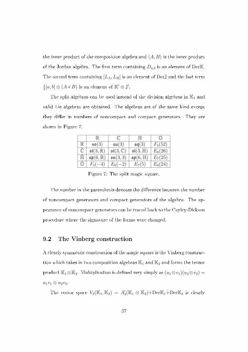
The split algebras can be used instead of the division algebras in K1 and
valid Lie algebras are obtained. The algebras are of the same kind except
they di�er in numbers of noncompact and compact generators. They are
shown in Figure 7.
R C H OR so(3) su(3) sq(3) F4(52)
C sl(3,R) sl(3,C) sl(3,H) E6(26)
H sp(6,R) su(3, 3) sp(6,H) E7(25)
O F4(−4) E6(−2) E7(5) E8(24)
Figure 7: The split magic square.
The number in the parenthesis denotes the di�erence between the number
of noncompact generators and compact generators of the algebra. The ap-
pearance of noncompact generators can be traced back to the Cayley-Dickson
procedure where the signature of the forms were changed.
9.2 The Vinberg construction
A clearly symmetric construction of the magic square is the Vinberg construc-
tion which takes in two composition algebras K1 and K2 and forms the tensor
product K1⊗K2. Multiplication is de�ned very simply as (u1⊗v1)(u2⊗v2) =
u1v1 ⊗ u2v2.
The vector space V3(K1,K2) = A′3(K1 ⊗ K2)+DerK1+DerK2 is clearly
37

symmetric with respect to the two composition algebras and it is a Lie algebra
once the Lie product is de�ned as follows. The vector space DerK1⊕DerK2 is
a Lie subalgebra. A′n(K1⊗K2) stands for n×n traceless (′) and antisymmetric
matrices over K1 ⊗K2.
Given two elements D ∈ DerK1 ⊕ DerK2 and A ∈ A′3(K1 ⊗ K2) in the
vector space, the action of D on A is such that [D,A], written D(A), is
the matrix on which the derivation algebras have acted element by element
where DerK1, naturally, acts on K1 of K1⊗K2 and DerK2 on K2 of K1⊗K2
alone.
For two elements A,B ∈ A′3(K1⊗K2), the Lie product is [A,B] = (AB−
BA)′+ 13
∑ij Daij ,bji where Dp⊗q,u⊗v = 〈p, u〉Dq,v + 〈q, v〉Dp,u. The �rst term
is the traceless part of an ordinary matrix commutator. The second term is
an element of the direct sum of derivations DerK1⊕DerK2 where aij and bji
are matrix elements and there is a sum over the indices.
9.3 The triality construction
The triality construction makes the Lie algebras as L3(K1,K2) = TriK1 ⊕
TriK2+3K1 ⊗K2 where the all-important Lie products will now be de�ned.
The signi�cance of 3K1⊗K2 is a direct sum of tensor products such that 3K1⊗
K2 is made up of elements (x1⊗ x2, y1⊗ y2, z1⊗ z2) where subscripts denote
which composition algebra the elements belong to. This direct product of
tensor product elements is then split into three terms themselves elements
like (x1⊗x2, y1⊗y2, z1⊗z2) such that F1(x1⊗x2)+F2(y1⊗y2)+F3(z1⊗z2) =
(x1 ⊗ x2, y1 ⊗ y2, z1 ⊗ z2).
38

Let T1 be an element of the �rst triality algebra, itself a triplet, (Tα1, Tα2, Tα3)
and T2 of the second triality algebra, also a triplet. The bars denote that the
element which the triality acts upon is conjugated before triality acting on it
and the result of the action is then again conjugated. The action of T1 can
only be on parts that have K1 so [T1, Fi(x1⊗x2)] = Fi(T1ix1⊗x2). Here, the
i in the subscript of T1i determines which element of the �rst triality triplet
acts.
Given two elements of the composition algebra, x and y, an element of the
triality algebra Tx,y = (4Sx,y, RyRx −RxRy, LyLx − LxLy) can be associated
where and the action of Sx,y(z) = 〈x, z〉y − 〈y, z〉x.
A map θ takes the triality triplet (A,B,C) and acts with combined
conjugation on the �rst and third element after cyclically permuting the
�rst to be the last: (B, C, A). The Lie product of two Fi and Fj is an
Fk (where ijk is a cyclic permutation of 123) [Fi(x1 ⊗ x2), Fj(y1 ⊗ y2)] =
Fk(y1x1 ⊗ y2x2), and when Fi(x1 ⊗ x2) acts on Fi(y1 ⊗ y2) then the result is
〈x2, y2〉θ1−iTx1,y1 + 〈x1, y1〉θ1−iTx2,y2 which is an element of TriK1⊕TriK2. If
i = 1 then θ1−i = θ0 = id, the identity map, and if i = 2 the inverse map θ−1
acts. For θ−2 the inverse map acts twice, as the notation suggests. This is
the content of the triality construction.
9.4 Maximal compact subalgebras
The maximal compact subalgebras of Lie algebras in the magic square are
shown in Figure 8. They can also be constructed by prescriptions based on
division algebras. [2][15]
39

R C H OR so(3) so(3) u(3) sq(3)⊕ so(3)C so(3) so(3)⊕ so(3) so(6) sq(4)H u(3) so(6) so(6)⊕ so(6) su(8)O sq(3)⊕ so(3) sq(4) su(8) so(16)
Figure 8: The maximal compact subalgebras.
10 Division algebras in supersymmetry
The dimensions of the division algebras 1, 2, 4 and 8 are also the dimensions of
the little groups of D = 3, 4, 6, 10 theories. Pure super Yang-Mills theories,
which have a gauge �eld A and a gaugino λ but no scalar �elds φ, only
exist in these dimensions. Superstrings also only exist in these dimension.
Depending on the dimension, the on-shell degrees of freedom of the super
Yang-Mills theory can therefore be described by either one octonion, one
quaternion, one complex number or one real number. This holds not only
for the vector but also for the spinor so that each is described by an element
of the same division algebra A. The work presented in the following sections
can be found in the recent publications of Du� et al. [1][2]
10.1 Spinors and vectors
The isomorphism so(1, 3) ∼= sl(2,C) states that space-time with the vector xµ
and Lorentz transformationsMµν can equally well be described by Hermitian
40

2× 2 matrices and their transformations such that
xµ =
x0
x1
x2
x3
↔ x =
x0 + x3 x1 − ix2
x1 + ix2 x0 − x3
, x′µ = Mµν x
ν ↔ x′ = AxA†.
In the new language, the Minkowski norm becomes the determinant and to
preserve the Minkowski norm, the Lorentz transformations represented by
the matrix A must be unimodular. The matrix x in which the space-time
vector is encoded, is partitioned into the Pauli matrices σ1, σ2, σ3 and the
identity matrix I such that x = x0I + x1σ1 + x2σ2 + x3σ3. This familiar case
is repeated because an unconventional extension follows.
The claim is now that just as so(1, 3) ∼= sl(2,C), and, in fact, so(1, 2) ∼=
sl(2,R), it also holds that so(1, 5) ∼= sl(2,H) and so(1, 9) ∼= sl(2,O). The
last statement, in particular, will need further elaboration, since, for in-
stance, AxA† is a product of three elements and possibly ambiguous for the
nonassociative octonions. So considering the D = n + 2-dimensional theory
means looking at so(1, n + 1) ∼= sl(2,A) where n is the dimension of the
corresponding division algebra A.
The appeal of the division algebra approach to describing so(1, n + 1)
is that the matrices stay 2 × 2 and the 2 × 2 matrix elements stay simple.
In D = 4 there is σµ = σµ = (−I, σ1, σ2, σ3) and σµ = σµ = (I, σ1, σ2, σ3)
where the middle two matrices σ1, σ2 will now be reconsidered. They are the
41

special case of the collection σµ = σµ = (−I, σa+1, σn+1) where
σa+1 =
0 e∗a
ea 0
=
0 1
1 0
,
0 −i
i 0
and σn+1 = σ3 =
1 0
0 −1
where, above, A = C and so n = 2, e0 = 1 and e1 = i. This means
that for A = H, two additional matrices are added where σ3 and σ4 that
look like σ2 but have units j or k instead where σ2 has i. These satisfy
σµσν +σν σµ = 2ηµνI and σµσν +σν σµ = 2ηµνI and can therefore be used to
generate space-time transformations of spinors and conjugate spinors.
A generalisation of the spinor transformation δΨ = 14λµνσµνΨ = 1
4λµνσµσνΨ
and that of the conjugate spinor transformation δΦ = 14λµν σµνΦ = 1
4λµν σµσνΦ
is now due. A priori, it cannot generalise directly since, in the octonionic
case, this will be a multiplication of more than two elements and is hence
generally ill-de�ned for octonions unless order of multiplication is provided.
If the generalisation of this expression is simple it could be that it is
(σ[µσν])Ψ or σ[µ(σν]Ψ). By counting alone, it can be seen that (σ[µσν]) cannot
add up to the 10 · 9/2 = 45 generators of SO(1, 9). The latter can be shown
to be the right ones by checking the commutation relations, considering the
action of the purported generators on an arbitrary octonion and �nding that
the commutation relations are those of the Lorentz algebra. The generators
are the octonionic operators
σµν (·) = 12[σµ(σν ·)− σν(σµ·)] and ˆσµν (·) = 1
2[σµ(σν ·)− σν(σµ·)] where (·)
is a slot for an octonion. The Hermitian matrix X associated with the vector
Xµ can be constructed as Xµσµ and X = Xµσµ = X − (TrX)I.
42

For sl(2,C), the transformation of X was δX = 14λµν(σµνX − Xσµν ).
The right transformation in sl(2,A) turns out to be δX = 14λµν(σµ(σνX) −
X(σµσν)). Since vectors can be constructed from spinors, this result can also
be derived from the spinor and conjugate spinor transformations alone.
Now, the little groups will be considered. As noted above, the on-shell
degrees of freedom of the spinor, conjugate spinor and vector representations
of SO(n), will each be represented by just one division algebra element.
Restriction to SO(n) transformations are made by setting the �rst and the
last element of the antisymmetric λ0µ = λ(n+1)µ = 0. It is convenient because
the transformations then only involve the generalised σ2 matrices and so
δΨ =1
4λµν σµνΨ =
1
4θab
e∗a(ebΨ1)
ea(e∗bΨ
2)
and the transformation of the spinor and the conjugate spinor can be read
o� directly as δΨ1 = δψ = 14θabe∗a(ebψ) and δΨ2 = δχ = 1
4θabea(e
∗bφ) where ψ
and χ were introduced in place of Ψ1 and Ψ2, respectively. For the vector,
the situation is analogous. The transformation is
δX =1
4θab
0 e∗a(ebx∗)− x∗(eae∗b)
ea(e∗bx)− x(e∗aeb) 0
such that δx = 1
4θab[ea(e
∗bx) − x(e∗aeb)] where x are the components of X
discounting the �rst and last component. This is frugal. Transformations
are formed by simply multiplying unit imaginary elements.
Recall that the multiplication of two division algebra elements is eaeb =
43

Γabcec and multiplication by a conjugated unit element e∗a is e∗aeb = Γabcec
where Γabc = (δa0δbc+δb0δac−δabδ0c+Cabc) and Γabc = (δa0δbc−δb0δac+δabδ0c−
Cabc). A multiplication of a division algebra element x by ea results in eax =
xbeaeb = xbΓabcec = ecΓ
acbxb which is a multiplication of the components of
x by a matrix. It was here used that Γabc = Γacb.
The structure constants satisfy ΓaΓb + ΓbΓa = 2δabI and ΓaΓb + ΓbΓa =
2δabI which imply that Σab = 12Γ[aΓb] and Σab = 1
2Γ[aΓb] are generators of
SO(n) in the spinor and conjugate spinor representations, respectively.
Likewise, an expansion of the vector x = xaea in the expression for δx
yields δx = eaθabxb from which can be deduced that J[ij]kl = δkiδjl − δkjδil .
The SO(n − 1) generators in the spinor and vector representations are
easily obtained. Simply disregard left multiplication by e0 such that there
is only eiea where a is allowed to range from 0 to 7 but i only from 1 to
7. This makes Γiab antisymmetric in the lower indices and they satisfy the
Cli�ord algebra of SO(n − 1) such that ΓiΓj + ΓjΓi = −2δijI so the gen-
erators are Σ[ij] = 12Γij = 1
2Γ[iΓj] and the spinors, conjugate spinors and
vectors transform as before except with the transformations consisting only
of multiplications by imaginary elements.
10.2 Dimensional reduction
The process of dimensional reduction can also be described using division
algebras. In the critical dimensionsD = 10, 6, 4, 3 the dimensional reduction
of spinors assumes a simple form on-shell. The decomposition of a spinor is
seen as a case of Cayley-Dickson construction. In D = 10 the spinor, written
44
as an octonion, decomposes into two spinors expressed as two quaternions in
D = 6, four spinors expressed as four complex numbers in D = 4 or eight
real numbers in D = 3.
The on-shell vector of D = 10, also written as an octonion, decomposes
into a vector of D = 6 expressed as a quaternion and four remaining com-
ponents identi�ed as scalars. The imaginary elements associated with the
scalar components disclose the existence of an internal symmetry. Upon
compacti�cation, the former space-time symmetry manifests itself as an in-
ternal symmetry.
Reducing the supersymmetry of the theory amounts to removing vectors
and spinors. These vectors and spinors are associated with imaginary divi-
sion algebra units and so it will turn out that reduction of supersymmetry
amounts to a consistent deletion of points in the Fano plane.
The N = 1 pure super Yang-Mills theory in D = 10 has two �elds,
the vector x and the superpartner spinor ψ that on-shell transform as rep-
resentations of SO(8). There is no internal symmetry here. All symmetry
is space-time symmetry. The vector and spinor are parameterised as octo-
nions such that xO = xaea and ψO = ψaea, respectively, which transform as
described before.
10.2.1 Reduction to six dimensions
In D = 6 and N = 2, the little group of the space-time symmetry is SO(4)
and there will be an internal symmetry that is also SO(4). Both can be
described as SU(2)× SU(2) ∼= SO(4) but SU(2) is also isomorphic to Sp(1)
which can be realised as a multiplication by imaginary quaternions. Recall
45

that the family sp(n) is generated by anti-Hermitian matrices of quaternions.
For n = 1, there is just one element in the matrix, an imaginary quaternion.
In total, the embedding is SO(8)st ⊃ (Sp(1)× Sp(1))st × (Sp(1)× Sp(1))int
where the subscript st denotes space-time symmetry and the subscript int de-
notes internal symmetry. Vectors decompose as 8v = (2,2;1,1) + (1,1;2,2)
whilst spinors decompose as 8s = (2,1;2,1) + (1,2;1,2). This will now be
realised with elements of division algebras. The vector xO is grouped and
renamed as
xO = x0 + x1e1 + x2e2 + x3e3 + x4e4 + x5e5 + x6e6 + x7e7
= (x0 + x4e4 + x5e5 + x7e7) + x1e1 + x2e2 + x3e3 + x6e6
= (x0 + x4e4 + x5e5 + x7e7) + φ1e1 + φ2e2 + φ3e3 + φ6e6
= xH + φHc .
where the subscript H refers to the quaternion subalgebra e0, e4, e5, e7 and
Hc is the associated quadrangle 6123. The spinor ψO is grouped and renamed
as
ψO = ψ0 + ψ1e1 + ψ2e2 + ψ3e3 + ψ4e4 + ψ5e5 + ψ6e6 + ψ7e7
= (ψ0 + ψ4e4 + ψ5e5 + ψ7e7) + e3(ψ3 + ψ6e4 + ψ2e5 + ψ1e7)
= (ψ0 + ψ4e4 + ψ5e5 + ψ7e7) + e3(χ3 + χ6e4 + χ2e5 + χ1e7)
= ψH + e3χH
which is an undoing (Cayley-Dickson) of the octonion into the quaternion
subalgebra e0, e4, e5, e7. The associated quadrangle is 6123. These refer
46

to the compacti�ed directions. Given that there has been a partitioning, it
is useful to consider what set multiplied elements of lines and quadrangles
belong to. Demarcate elements on the line with a hat ( ) and elements
on the quadrangle with a check ( ). When referring to imaginary elements
alone subscripts or superscripts i and j will be used. Two units on the line
multiplied together give units on the line eaeb = Γabcec. They sit in the
quaternion subalgebra. A unit on the quadrangle multiplied by a unit on the
line gives units on the quadrangle eaeb = Γabcec. Two units on the quadrangle
multiplied give units on the line eaeb = Γabcec. In short, lines map objects
into themselves and quadrangles map into opposite objects.
Given that e3 has been singled out it is also useful to consider its prod-
ucts with the other elements. Unambiguous left multiplication of −e3 on
both sides of e3ea = Γ3abeb gives ea = −e3Γ3
abeb, and, similarly, for the quad-
rangle elements, ea = −e3Γ3abeb. It is in both cases unambiguous with no
parentheses needed because only two imaginary elements are involved.
Now, the transformations of the spinor and vector will be considered.
The transformation parameters θab are split as θab, θab and θab but with
θab = 0. The transformation of the spinor ψO proceeds as follows. The
starting point is the D = 10 space-time transformation which is split into
lines and quadrangles. The transformation of the spinor is
δψO =1
4θabe∗a(ebψO)
=1
4θabe∗a(ebψO) +
1
4θabe∗a(ebψO)
=1
4θabe∗a(eb(ψcec + e3χcec)) +
1
4θabe∗a(eb(ψcec + e3χcec))
47

where the split into internal and space-time parameters was made in go-
ing from second line to third line. Notice that the �rst term containing
e∗a(eb(ψcec) has space-time indices only so the multiplication is amongst el-
ements of the associative quaternion subalgebra and therefore the paren-
theses can be moved to group the unit elements (e∗aeb)ψcec, abbreviated as
ustψH. An important identity that is useful here is that eb(e3ec) = e3(e∗bec).
This can be used to manipulate the second term to pull e3 out to the left
such that it becomes e3(uotherst χH) where uother
st refers to some product of unit
elements associated with space-time. The third term is manipulated into
θabe∗a(ebec) = θabec(e∗aeb), which can be checked to hold. It is a reordering
that frees the space-time unit and displaces the internal indices and multi-
plies them with one another, abbreviated as ψHuint. The last manipulation,
the manipulation of 14θabe∗a(e3χcec) is the most nontrivial. The resort is to
write the product in terms of structure constants and reorder them by using
the fact that they obey the Cli�ord algebra and by also using the aforemen-
tioned identity involving Γ3 to eventually separate and order e3 to be on the
far left. The net e�ect of these manipulations is e3(χHuotherint ).
The transformations should of the form δψO = δψH + e3δχH which ex-
plains why it was important to manipulate the expressions to get e3 sepa-
rated and on the far left. The transformations are δψH = ustψH + ψHuint
and δχH = uotherst χH + χHu
otherint where ust and uint turn out to be imaginary
unit quaternions and uotherst and uother
int turn out to be other imaginary unit
quaternions.
This establishes that ψ and χ transform as representations of (Sp(1) ×
Sp(1))st × (Sp(1) × Sp(1))int. As stated earlier, the left or right action of
48

imaginary quaternions is isomorphic to Sp(1). The action of the four Sp(1)
in (Sp(1)×Sp(1))st×(Sp(1)×Sp(1))int correspond to ust, uotherst , uint and u
otherint ,
respectively. The in�nitesimal transformation of an object that transforms
as a tensor product is a sum of terms where each term corresponds to a factor
of the tensor product and is a multiplication of the object with that factor
alone. The conclusion is that ψ transforms under the �rst and third Sp(1)
and χ transforms under the second and fourth Sp(1) as anticipated.
The transformation of the vector proceeds in a similar way and starts
with the full space-time transformation δxO = 14θab(ea(e
∗bxO) − xO(e∗aeb))
which after the split of the vector and the transformation parameters into
internal and space-time parts xaea + φaea is also
δx =1
4θab(ea(e
∗baO)− aO(e∗aeb)) +
1
4θab(ea(e
∗baO)− aO(e∗aeb))
=1
4θab(ea(e
∗b(xcec + φcec)))− (xcec + φcec)(e
∗aeb))
+1
4θab(ea(e
∗b(xcec + φcec)))− (xcec + φcec)(e
∗aeb))
= (uotherst xcec − xcecuint) + e3(uother
int φcec − φcecuint) = δxH + e3δφH
where in the last line the same identi�cations of unit imaginary quaternions
were made, but as can be seen, the imaginary elements are di�erently ar-
ranged. They are arranged in such a way that, unlike the spinor, only imagi-
nary unit quaternions associated with space-time transformations transform
the vector and only imaginary unit quaternions associated with the internal
transformations act on the scalars. As anticipated, the vector only trans-
forms under the �rst and second of (Sp(1) × Sp(1))st × (Sp(1) × Sp(1))int
49

corresponding to ust and uotherst whilst the scalars only transform under the
third and fourth Sp(1) corresponding to uint and uotherint .
10.2.2 Reduction to four dimensions
The more intricate decomposition is the reduction from D = 10 and N = 1
to D = 4 and N = 4. The SO(8)st space-time symmetry becomes an SO(2)st
space-time symmetry and an SO(6)int internal symmetry. The original D =
10 vector is decomposed into a D = 4 vector and six scalars. The original
D = 10 spinor is decomposed into four spinors. SO(6)int is also isomorphic
to SU(4)int and, as is well-known, SO(2)st is isomorphic to U(1)st.
The decomposition of the vector representation is to the U(1)st neutral
second rank antisymmetric representation of SU(4)int and two singlets, one
singlet with charge one and the other with charge minus one: 8v = 60 +
11 +1−1. The spinor decomposes into the fundamental and antifundamental
representation of SU(4)int with opposite charges of one half: 8s = 41/2+4−1/2.
The starting point is again the octonion vector xO which is split into a
subalgebra xO = xC + φCc = xaea + φbeb = (x0 + x3e3) + φ1e1 + φ2e2 +
φ4e4 + φ5e5 + φ6e6 + φ7e7 where, now, a = 0, 3 and b = 1, 2, 4, 5, 6, 7. The
vector is represented by a complex number and six scalars associated with the
remaining six imaginary elements. The original octonion spinor is split into
four spinors, each represented by a complex number. The original octonion
spinor e�ectively becomes a quaternion over the complex numbers:
ψO = (ψC)aea = (ψ0+e3ψ3)+(ψ4+ψ6e3)e4+(ψ5+ψ2e3)e5+(ψ7+ψ1e3)e7 =
(ψC)aea where a = 0, 4, 5, 7 is a basis for quaternions, each element now a
complex number ψC.
50

The e�ect of multiplying the octonion spinor by an imaginary unit that
is internal, ei, conjugates the complex components of the quaternion and in
addition multiplies them by a 4 × 4 matrix Υiab
whose commutator with a
complex conjugated Υ∗jab
= Υj
abturn out to be one of the 6 · 5/2 = 15
Hermitian and traceless generators of SU(4). There are 6 elements in the set
i = 1, 2, 4, 5, 6, 7 and so there are 6 · 5/2 = 15 commutators (generators).
Since the matrices are furthermore 4 × 4, this means that this is the fun-
damental representation of SU(4). The generators in the antifundamental
representations are obtained by conjugating these generators.
The transformation parameters θab are again divided into θab, θab and
θab = 0. The spinor transformation is δψO = 14θabe∗a(ebψO) = 1
2θ03e3(ψaCea) +
14θije∗i (ej(ψ
aCea)) = 1
2θ03e3ψ
aCea − 1
2θij(T
[ij]
abψbC)ea
The spinor transforms by left multiplications of two unit elements, where
the last unit multiplied is conjugated. Each multiplication by an imagi-
nary element produces a factor of Υ, one of them conjugated. Since the
transformation parameters are antisymmetric θab, this matrix product is an-
tisymmetrised and therefore generates SU(4) in the fundamental represen-
tation. For the space-time transformation there is only one parameter θ03.
The spinor is multiplied by 12e3 which is an in�nitesimal transformation of
U(1) with positive charge 12. In total, the complex spinor ψaC transforms as
41/2 + 4−1/2 of SU(4)int × U(1)st as anticipated. One term comes from the
real part and the other term from the imaginary part of the complex number.
The octonion vector transforms as δaO = 14θab(ea(e
∗baO) − aO(e∗aeb)) =
12θ03(−e3aC − aCe3) + 1
2θ03(−e3φCc − φCce3) + 1
4θij(ei(ejaC) − aC(e∗i ej)) +
14θij(ei(ejφCc)−φCc(e∗i ej)) = −θ03e3aC + 1
2θijelJ[ij]lkφk which establishes that
51

the vector transforms according to 11 + 1−1 of SU(4)int × U(1)st and the
scalars according to 60. Instead of looking for the second rank antisymmet-
ric representation of SU(4) the vector representation of SO(6) was identi�ed
as the representation that the scalars transform according to.
Admittedly, some steps have been omitted in this derivation which is more
of a sketch of a derivation. The reader has already seen enough manipulations
with division algebra elements and a full-�edged derivation of the above
would be very detailed and as a result too tedious to read.
10.2.3 Reduction to three dimensions
The simplest reduction is the reduction from D = 10 to D = 3 since, here,
the space-time symmetry is trivial. The decomposition of SO(8)st is into
SO(7)int. The spinor of SO(8)st becomes the spinor of SO(7)int such that
8s = 8. The vector of SO(8)st becomes a vector and a singlet of SO(7)int
such that 8v = 7 + 1.
The vector xO is trivially split as xO = xR + φRc = x0 + φiei, the spinor
is expressed as ψO = (ψR)aea = ψaea and the transformation parameters θab
are split as θ0i and θij. As before, θ0i = 0. The transformations are δψO =
14θije∗i (ejea)ψa and δxO = 1
4θij(ei(e
∗jekφk) − φkek(e
∗i ej) but it was already
mentioned in a previous section that by restricting the spinor and vector
transformations to only involve imaginary unit elements are transformations
of spinors and vectors of SO(n− 1) are obtained, which here is SO(7).
It can also with a tedious but straightforward computation using the
structure constants be shown, directly, that δψa = −12θijΣ
[ij]abψb and δφl =
12θijJ[ij]lkφk which is a spinor and vector transformation of SO(7), respec-
52

tively. Though elementary, such computations can easily occupy whole sheets
of paper.
10.2.4 Reduction of supersymmetry
A theory in D = 10 and N = 1 was the starting point. Each step down
doubles the supersymmetry such that D = 6 gives N = 2, D = 4 gives
N = 4 and D = 3 gives N = 8. These are the maximal supersymmetries.
For each step down, the spinor splits into two spinors of the lower-dimensional
theory. This is the Cayley-Dickson procedure in reverse.
The content of nonmaximal supersymmetries can also be obtained using
the division algebra formalism. Think about the truncation in terms of the
spinors. In order to halve the supersymmetry in D = 6, a quaternion subal-
gebra must be preserved and four imaginary elements must be removed. This
corresponds to a deletion of those components associated with the quadran-
gle 3612 from ψO = (ψ0 +ψ4e4 +ψ5e5 +ψ7e7)+e3(χ3 +χ6e4 +χ2e5 +χ1e7)→
ψ0 + ψ4e4 + ψ5e5 + ψ7e7. For the vector, xO = (x0 + x4e4 + x5e5 + x7e7) +
φ1e1 +φ2e2 +φ3e3 +φ6e6 → x0 +x4e4 +x5e5 +x7e7. There is nothing special
about this quadrangle. What is important is that it is the quadrangle corre-
sponding to the quaternion algebra that will be preserved. An equal number
of bosonic degrees of freedom φa will also disappear. One is left with a line
in the Fano plane and hence a theory de�ned over the quaternions.
In obtaining a D = 4 and N = 2 theory from D = 4 and N = 4 theory,
two of the four spinors are removed. The quadrangle 5271 may be chosen such
that ψO = ψaCea = (ψ0+e3ψ3)+(ψ4+ψ6e3)e4+(ψ5+ψ2e3)e5+(ψ7+ψ1e3)e7 →
(ψ0 + e3ψ3) + (ψ4 + ψ6e3)e4 and, correspondingly, for the vector xO = (x0 +
53

x3e3) + φ1e1 + φ2e2 + φ4e4 + φ5e5 + φ6e6 + φ7e7 → (x0 + x3e3) + φ4e4 + φ6e6.
A further reduction is to remove 46 which leaves only one spinor and one
vector and gives a D = 4 and N = 1 theory.
In the case of D = 3, the di�erence is that all imaginary elements can be
deleted. Deleting a quadrangle brings it to N = 4, deleting two imaginary
elements to N = 2 and deleting the last imaginary element gives N = 1
which is a rather uninteresting theory.
10.3 Super Yang-Mills
The dimensional reductions and truncations of supersymmetry of an N = 1
and D = 10 pure super Yang-Mills theory done in the preceding section sug-
gest that two division algebras AN and An can be used to specify a pure su-
per Yang-Mills theory with extended, possibly nonmaximal, supersymmetry.
The on-shell degrees of freedom were described by an element of a division
algebra An. In D = 4, An was C. The vectors and spinors were here rep-
resented by complex numbers. The maximal supersymmetry is in this case
N = 4 and the spinor, originally an octonion, was rewritten (in the manner
of the Cayley-Dickson procedure) as a complex-valued quaternion H ⊗ C.
Truncation of supersymmetry from N = 4 to N = 2 amounted to deleting
two of the three imaginary elements associated with the quaternion resulting
in a complex algebra that can thus be associated with N = 2. This suggests
that a division algebra AN also be associated with extended supersymmetry
such that N = 1, 2, 4, 8 correspond to R, C, H and O, respectively. An
oxidation algebra2 AnN can be associated with the two algebras An and AN .2There was no name for it in the article [1] so this is my suggestion.
54

Before truncation of supersymmetry was considered this oxidation algebra
was always O. An overview is given in Table 9. Before introducing trunca-
(D,N ) 1 2 4 810 OR ∼ O6 HR ∼ H HC ∼ O4 CR ∼ C CC ∼ H CH ∼ O3 RR ∼ R RC ∼ C RH ∼ H RO ∼ O
Figure 9: Division algebra formulations of n+2-dimensional super Yang-Millstheories with N = 1,2,4,8.
tion of supersymmetry, only the theories with maximal supersymmetry were
dealt with, corresponding to the theories in the diagonal. Dimensional re-
duction is a step down the rows and a truncation of supersymmetry is a step
to the left.
Before proceeding to theories of supergravity, triality will �rst be dis-
cussed. It was a component in the later manifestly symmetric magic square
constructions and it was introduced as a triplet of so(n) elements (A,B,C)
for which it holds that A(xy) = (Bx)y + x(Cy) for all x, y ∈ A but this
sounds very abstract with no clear physical picture. One way to think about
triality is in the following manner. A spinor and a conjugate spinor can be
used to form a vector x = χψ∗ = χbψcΓabcea, or a spinor can be made from
a vector and a conjugate spinor ψ = x∗χ = xaχcΓabceb, or a conjugate spinor
can be made from a vector and a spinor χ = xaψcΓabceb. Supposing that all
three objects x, χ, ψ∗ are then transformed such that δx = A(x), δχ = B(χ)
and δψ∗ = C(ψ∗), then, still insisting that x is made from ψ and χ, these
transformations would have to be related, and their relation is such that A,
B, and C satisfy δx = A(x) = δ(χψ∗) = (δχ)ψ∗+χ(δψ∗) = (Bχ)ψ∗+χ(Cψ∗)
55

which is exactly the condition that de�nes triality! These triality algebras
exactly match the symmetries of the g = 0 Lagrangian of D = 3 super
Yang-Mills. [1]
Super Yang-Mills theories were identi�ed using two division algebras so
the triality de�nition is unde�ned for cases when there is more than one
division algebra involved. The D = 3 case is an extreme case where space-
time symmetry is trivial. A generalisation is needed. It turns out that
to get the full symmetries of the Lagrangian of any super Yang-Mills theory
discussed here it su�ces to consider a subset of the oxidation algebra AnN re-
stricted such that the transformations of the vector Amust respect the space-
time symmetry of the vector: Tri(AnN ,An) = {(A,B,C) ∈ so(n)|A(xy) =
B(x)y + xC(y), A(An) ⊆ AnN = An}. [1]
10.3.1 Lagrangians
Brie�y, attention will now be turned to the super Yang-Mills Lagrangian. It
will not be treated in detail but merely presented. Supersymmetry transfor-
mations will be introduced, written using division algebra elements.
The n + 2-dimensional N = 1 super Yang-Mills theory has a gauge �eld
A Aµ and a spinor �eld ΨA that transform as the adjoint representation of
a gauge group G where A = 0, . . . , dim(G). The �eld strength is F Aµν =
∂µAAν −∂νA A
µ +gf ABC A B
µ A Cν and the covariant derivative acts as DµΨA =
∂µΨA + gf ABC A B
µ ΨC .
As discussed earlier, the spinor is an element of sl(2,An). It is furthermore
a Grassmann variable, so the division algebras used here are not de�ned over
the real numbers but rather over Grassmann variables. The Lagrangian needs
56

a kinetic spinor term that is real, invariant under space-time transformations
and bilinear. One such product is given by Re(iΨ†Φ) = i2(Ψ†Φ − Φ†Ψ),
adapted here as Re(iΨ†σµ∂µΨ). There is no ambiguity in having a multipli-
cation of three division algebra elements here since the associator is purely
imaginary and only the real part is considered so any reordering of multipli-
cation order would contribute with an associator whose real part is trivially
zero.
The action is
S =
∫d(n+2)x
(−1
4F Aµν F A
µν − Re(iΨ†AσµDµΨA
)). (10.3.1)
The supersymmetry transformations are δA Aµ = Re(iΨ†Aσµε) and δΨ
A =
12F ε where F = Fµν σ
µν . Packaged as a matrix, the supersymmetry transfor-
mation of the vector is δAA = δA Aµ σµ = i(ΨAε† − εΨ†A).
The action of the general super Yang-Mills theory associated with an
algebra An and an oxidation algebra AnN is
S(An,AnN ) =
∫dx(n+2)
(− 1
4F Aµν F A
µν −1
2Dµφ
∗ADµφA
− Re(iΨ†AσµDµΨA)− gf ABC Re(iΨ†AεφBΨC)
− 1
16g2f A
BC f ADE (φ∗BφD + φ∗DφB)(φ∗CφE + φ∗EφC)
)(10.3.2)
where ε is a 2× 2 matrix like the Pauli matrix σ2 but without the imag-
inary elements. Vectors decompose as AAnN = AAn + φAcnε where the sub-
script An refers to the subalgebra of the division algebra corresponding to
57

space-time symmetry and Acn refers to the remaining elements, that is to
say, the elements complementary to An. The supersymmetry transforma-
tions become δAA = i(ΨAε† − εΨ†A)An , δφA = − i
2Tr(ε(ΨAε† − εΨ†A
)Acn
)and δΨA = 1
2FAε+ 1
2σµε(Dµφ
Aε) + 14f ABC φC(φBε).
The proof of supersymmetry on-shell turns out to rest on the alternativ-
ity of the algebra which is a property shared by all division algebras. [12]
O�-shell, closure of the supersymmetry algebra requires addition of aux-
iliary �elds. The spinor has dimension 2n and the vector has dimension
n+2−1 = n+1. In total, 2n− (n+2−1) = n−1 additional degrees of free-
dom are needed. The counting suggests that an imaginary division algebra
element carrying scalars be added. The usual nondynamical term associated
with these scalar �elds is added to the action. A careful analysis �nds that,
unless this �eld transforms according to the fundamental representation of
G2, the supersymmetry transformations break the Lorentz invariance of the
theory. For quaternions the auxiliary �elds must transform as the adjoint
representation of Sp(1). [1]
To further obtain closure of the supersymmetry algebra in D = 10, the
supersymmetry parameter, the spinor ε, must be restricted to have its �rst
component ε1 have no imaginary part. This restriction is ultimately due to
the nonassociativity of the octonions. [1] Associators which are nontrivial
for the octonions obstruct the closure. The o�-shell closure of the D = 10
supersymmetry algebra is intricate but the octonions elucidate its failure and
subsequent patching.
58

10.4 Supergravity and the magic square
In more than one context theories of supergravity arise from (tensor products
of) super Yang-Mills theories. The multiplets of D = 10 Type IIA and
Type IIB supergravity can be obtained from a tensor product of D = 10
super Yang-Mills multiplets. [24] The di�erence between Type IIA and Type
IIB supergravity is then whether or not the same spinor representation was
used in both the left and right super Yang-Mills multiplets. Type IIA is
nonchiral whilst Type IIB is chiral. Before proceeding to construct theories
of supergravity from theories of super Yang-Mills using division algebras the
construction of Type IIA from two D = 10 super Yang-Mills theories will be
presented.
Dynkin labels will be used in the following to denote irreducible rep-
resentations. The irreducible representations of D4 are denoted [1, 0, 0, 0]D4
(fundamental representation), [0, 1, 0, 0] (adjoint representation), [0, 0, 1, 0]D4
(spinor representation), [0, 0, 0, 1]D4 (conjugate spinor representation) and
[0, 0, 1, 1]D4 (third rank antisymmetric representation). The irreducible rep-
resentations of B4 are denoted [1, 0, 0, 0]B4 (fundamental representation),
[0, 1, 0, 0]B4 (adjoint representation), [0, 0, 1, 0]B4 (third rank antisymmetric
representation) and [0, 0, 0, 1]B4 (spinor representation).
The D = 11 supergravity which is understood as the infrared limit of
M-theory with SO(9) as the little group has a graviton [2, 0, 0, 0]B4 , a grav-
itino [1, 0, 0, 1]B4 and a 3-form [0, 0, 1, 0]B4 . Dimensional reduction of the
graviton to D = 10 where the little group is SO(8) gives [2, 0, 0, 0]D4 +
[1, 0, 0, 0]D4+[0, 0, 0, 0]D4 which is another graviton, a gauge �eld and a scalar.
59

The gravitino [1, 0, 0, 1]B4 reduces to two gravitinos with opposite chirality
[1, 0, 0, 1]D4 +[1, 0, 1, 0]D4 and two fermions [0, 0, 1, 0]D4 +[0, 0, 0, 1]D4 . The 3-
form [0, 0, 1, 0]B4 reduces to [0, 0, 1, 1]D4 +[0, 1, 0, 0]D4 , a 3-form and a 2-form.
The resulting D = 10 theory is the Type IIA supergravity with the �eld
content [2, 0, 0, 0]D4 + [1, 0, 0, 0]D4 + [0, 0, 0, 0]D4 + [1, 0, 0, 1]D4 + [1, 0, 1, 0]D4 +
[0, 0, 1, 0]D4 + [0, 0, 0, 1]D4 + [0, 0, 1, 1]D4 + [0, 1, 0, 0]D4 .
The D = 10 super Yang-Mills theory whose little group is SO(8) has a
vector [1, 0, 0, 0]D4 and a spinor [0, 0, 1, 0]D4 or a conjugate spinor [0, 0, 0, 1]D4 .
When performing the tensor product of two super Yang-Mills multiplets, a
left one ([1, 0, 0, 0] + [0, 0, 1, 0]) and a right one ([1, 0, 0, 0] + [0, 0, 0, 1]), the
result is the �eld content of Type IIA supergravity. There are four tensor
products to be computed. The �rst tensor product [1, 0, 0, 0][1, 0, 0, 0] =
[2, 0, 0, 0] + [0, 1, 0, 0] + [0, 0, 0, 0] gives the NS-NS sector. The tensor product
[0, 0, 1, 0][0, 0, 0, 1] = [0, 0, 1, 1] + [1, 0, 0, 0] is the R-R sector. The last two
parts are [1, 0, 0, 0][0, 0, 0, 1] = [1, 0, 0, 1]+ [0, 0, 1, 0] and [1, 0, 0, 0][0, 0, 1, 0] =
[1, 0, 1, 0] + [0, 0, 0, 1]. Collecting all terms gives the Type IIA supergravity
[2, 0, 0, 0]+[0, 1, 0, 0]+[0, 0, 0, 0]+[0, 0, 1, 1]+[1, 0, 0, 0]+[1, 0, 0, 1]+[0, 0, 1, 0]+
[1, 0, 1, 0]+ [0, 0, 0, 1]. The chiral Type IIB theory arises from considering the
product ([1, 0, 0, 0] + [0, 0, 1, 0])([1, 0, 0, 0] + [0, 0, 1, 0]).
Other work has looked at relating supergravity scattering amplitudes to
scattering amplitudes of super Yang-Mills theories. [25]
Also, given that the infrared limit of a string theory is a theory of su-
pergravity it is not unreasonable to expect a manifestation of the relations
between supergravity and super Yang-Mills in string theory as well. In-
deed, that turns out to be the case. Relations exist, the KLT relations, that
60

describe closed string tree amplitudes (gravity) as products of open string
(gluon) tree amplitudes. [26]
Obtaining supergravity �elds by a tensor product of super Yang-Mills
�elds will now be done in D = 3. The graviton and gravitino have D · (D −
3)/2 = 0 degrees of freedom. 2-forms have (D− 2)(D− 1)/(2 · 1) = 1 degree
of freedom and are hence dual to scalars. It has already been shown how
the super Yang-Mills �elds are formulated with division algebras so all that
needs to be done is perform the tensor product of two division algebras AL
and AR. The spinors are not division algebras over the real numbers but
division algebras over Grassmann variables. The D = 3 supergravity �elds
as tensor products of super Yang-Mills �elds are listed in Figure 10.
AL/AR (Aµ)R ∈ ReAR φR ∈ ImAR λR ∈ AR(Aµ)L ∈ ReAL gµν + ϕ ∈ ReAL ⊗ ReAR ϕ ∈ ReAL ⊗ ImAR Ψµ + χ ∈ ReAL ⊗ ARφL ∈ ImAL ϕ ∈ ImAL ⊗ ReAR ϕ ∈ ImAL ⊗ ImAR χ ∈ ImAL ⊗ ARλL ∈ AL Ψµ + χ ∈ AL ⊗ ReAR χ ∈ AL ⊗ ImAR ϕ ∈ AL ⊗ AR
Figure 10: The �elds of supergravity as tensor products of super Yang-Mills�elds.
The supersymmetry of the resulting supergravity N is equal to the sum of
supersymmetries of the respective super Yang-Mills theories N = NL +NR.
The gravitino is grouped such that Ψµ =
AL ⊗ ReAR
ReAL ⊗ AR
∼=AL
AR
and
gµν ∈ R. The spinors and scalars are grouped so that ϕ, χ =
AL ⊗ AR
AL ⊗ AR
.
The three-dimensional theory has a trivial space-time symmetry and only
internal symmetry. The former space-time symmetry manifests itself as in-
ternal symmetry as a result of compacti�cation. As a result of toroidal com-
pacti�cation, hidden symmetries of the theory known as U-dualities appear.
61

It may be seen as a generalisation of electromagnetic duality. U-dualities
also appear in string theory where they are combinations of T-duality and
S-duality mixing radii and couplings. [27]
In contrast to dimensional reduction, oxidation goes the other way and at-
tempts to identify the higher-dimensional theory from which a lower-dimensional
theory originates. The highest-dimensional theory that a low-dimensional
one comes from is called the oxidation endpoint. The U-duality groups de-
pend on this oxidation endpoint. For theories whose oxidation point is the
D = 11 supergravity, the exceptional groups E6, E7 and E8 arise as U-duality
groups in dimensions D = 5, 4, 3, respectively. [17] The U-duality groups of
theories in D = 3, 4, 5 whose oxidation points are D = 11, 10, 9 supergravity
form a subsquare of the magic square! However, one slot of the magic square
containing the F4 does not appear in this scheme of dimensional reduction.
A whole magic square of theories of supergravity has been found using the
approach outlined in this dissertation. [2] The rows and columns of this magic
square, which are associated with the four division algebras, are identi�ed
with left and right super Yang-Mills theories where each cell in the magic
square, a symmetry, corresponds to the U-duality group of the supergravity
theory that arises as a tensor product of the respective super Yang-Mills
theories (division algebras).
A magic square construction that treats the left and right division alge-
bras AL and AR symmetrically has been crucial to this identi�cation. As has
been described, the triality construction is a construction of the magic square
that is manifestly symmetric in its two parameters. Furthermore, the triality
algebras on their own have been associated with full symmetries of super
62

Yang-Mills theories. Using the triality construction, but modi�ed in some
of the commutators using the Weyl unitary trick to get the right number of
noncompact and compact generators, L3 = Tri(AL)⊕ Tri(AR)+3(AL ⊗ AR)
gives the U-duality groups shown in Figure 11.
R C H OR N = 2
f = 4G = SL(2,R)H = SO(2)
N = 3f = 8G = SU(2, 1)H = SU(2) ×SO(2)
N = 5f = 16G = USp(4, 2)H = USp(4) ×USp(2)
N = 9f = 32G = F4(−20)
H = SO(9)
C N = 3f = 8G = SU(2, 1)H = SU(2) ×SO(2)
N = 4f = 16G = SU(2, 1)2
H = SU(2)2 ×SO(2)2
N = 6f = 32G = SU(4, 2)H = SU(4) ×SU(2)× SO(2)
N = 10f = 64G = E6(−14)
H = SO(2) ×SO(10)
H N = 5f = 16G = USp(4, 2)H = USp(4) ×USp(2)
N = 6f = 32G = SU(4, 2)H = SU(4) ×SU(2)× SO(2)
N = 8f = 64G = SO(8, 4)H = SO(8) ×SO(4)
N = 12f = 128G = E7(−5)
H = SO(12) ×SO(3)
O N = 9f = 32G = F4(−20)
H = SO(9)
N = 10f = 64G = E6(−14)
H = SO(2) ×SO(10)
N = 12f = 128G = E7(−5)
H = SO(12) ×SO(3)
N = 16f = 256G = E8(8)
H = SO(16)
Figure 11: Supergravity theories with extended supersymmetry N , f degreesof freedom, U-duality groups G and their maximal compact subgroups H.
The U-duality group G is a global symmetry of the theory and H which
is the maximal compact subgroup of G is a local symmetry. The scalars of
the theory parameterise cosets G/H. In the special case of R⊗O, the scalars
are points in a genuine projective plane, the aforementioned Moufang plane
OP2. Save the scalars, the �elds transform as representations of H.
The supergravity theories with N > 8 are pure. The supergravity the-
ories with N ≤ 8 are coupled to matter such that the squaring to get
N = 2, 3, 4, 5, 6, 8 supergravity theories gives supergravity coupled to an
63

additional k = 1, 1, 2, 1, 2, 4 matter multiplets, respectively.
This construction is not directly applicable to supergravity theories in
D = 4, D = 6 and D = 10 theories. The method works in D = 3 because the
space-time symmetry is trivial and therefore, e�ectively, the triality algebras
only depend on one division algebra, which is what the triality construc-
tion of the magic square requires. A generalisation of the triality algebra
Tri(AnN ,An) has been introduced in a previous section to account for the
full symmetries of super Yang-Mills theories, but a construction that yields
the U-duality groups of the higher-dimensional supergravity theories is still
under development. Such a construction will depend on three division al-
gebras. One division algebra will account for the space-time symmetry, one
division algebra for the left super Yang-Mills theory and one for the right
super Yang-Mills theory. In D = 4, the division algebra associated with the
supersymmetry of the super Yang-Mills theory is at most the quaternion al-
gebra so the square at this level is a 3 × 3 square. In D = 6, the division
algebra is at most the complex algebra and so the supergravity theories that
can be made form a 2 × 2 square. In D = 10, the division algebra associ-
ated with the supersymmetry is real (trivial) and there is only one theory.
This pyramidal collection of supergravity theories parameterised by the three
division algebras, has been dubbed a magic pyramid.
11 Summary
The division algebras were introduced. They were then constructed in a
uni�ed manner in accordance with the Cayley-Dickson procedure. The prop-
64

erties of the quaternions were discussed. The properties of the octonions
were then discussed. Split algebras were constructed and listed using a mod-
i�ed Cayley-Dickson procedure. Jordan algebras were brie�y introduced and
classi�ed. A description of root lattices of interesting Lie algebras were then
described using integral division algebra elements. Considering only root lat-
tices, an informal hint of a magic square was noted. Relevant subalgebras
of algebras and their maps were then described. These subalgebras were
then used to construct the magic square. The Tits-Freudenthal, Vinberg
and triality constructions of the magic square were then presented. Finally,
recent work of the department was described. After introducing space-time
transformations described using division algebra elements symmetries, di-
mensional reductions and truncations of supersymmetry of super Yang-Mills
theories were described using division algebras. Supergravity theories were
then constructed as tensor products of super Yang-Mills theories. A magic
square of supergravity theories was found. It was discussed how this can be
extended to a magic pyramid of supergravity theories.
12 Outlook
A generalisation of the magic square, the magic pyramid, is not yet complete
since a generalisation of the magic square triality construction is needed, pos-
sibly involving the new triality algebra de�nition. Lagrangians of supergrav-
ity theories described as elements of division algebras and the Lagrangians
of dimensionally reduced theories have not yet been developed. These are
under development.
65

It was noted that the exceptional Jordan algebra has a relation to SO(9)
(and possibly SO(26) through F4) which is the stability group of quan-
tum states in octonionic quantum mechanics. The little group of an 11-
dimensional theory is also SO(9) and these Poincare transformations leave
a quantum state with a particular momentum invariant. Interestingly, the
Standard Model was found to also arise as the stability group after a joint F4
and a unidrectional SO(9) transformation. Although no major results have
emerged from these considerations, physically relevant groups do appear.
These could be further hints of something signi�cant yet to be discovered in
these octonionic structures.
Division algebras failed to explain, �rst, isospin and, later, quark struc-
ture. Maybe they describe an even deeper layer, and maybe that deeper layer
is string theory or M-theory.
66

13 References
[1] A. Anastasiou, L. Borsten, M. J. Du�, L. J. Hughes, and S. Nagy,
�Super Yang-Mills, division algebras and triality,� arXiv:1309.0546
[hep-th].
[2] L. Borsten, M. J. Du�, L. J. Hughes, and S. Nagy, �A magic square
from Yang-Mills squared,� arXiv:1301.4176 [hep-th].
[3] L. Borsten, D. Dahanayake, M. J. Du�, H. Ebrahim, and W. Rubens,
�Black holes, qubits and octonions,� Physics Reports 471 (2009)
113�219. Issues 3�4.
[4] S. Okubo, Introduction to Octonion and Other Non-Associative
Algebras in Physics. Cambridge University Press, 1995.
[5] G. M. Dixon, Division Algebras: Octonions, Quaternions, Complex
Numbers and the Algebraic Design of Physics. Kluwer Academic
Publishers, 2010.
[6] P. Lounesto, Cli�ord Algebras and Spinors. London Mathematical
Society, 2001.
[7] F. Gursey and C.-H. Tze, On the role of division, Jordan and related
algebras in particle physics. World Scienti�c, 1996.
[8] K. McCrimmon, A Taste of Jordan Algebras. Springer, 2004.
[9] M. Gunaydin and F. Gursey, �Quark structure and octonions,� J.
Math. Phys. 14 (1973) 1651�1667.
67

[10] T. Kugo and P. Townsend, �Supersymmetry and the division algebras,�
Nuclear Physics B 221 (1983) 357�380.
[11] J. M. Evans, �Supersymmetric yang-mills theories and division
algebras,� Nuclear Physics B 298 (1988) 92�108.
[12] J. C. Baez and J. Huerta, �Division algebras and supersymmetry I,�
arXiv:0909.0551 [hep-th].
[13] J. C. Baez and J. Huerta, �Division algebras and supersymmetry II,�
arXiv:1003.3436 [hep-th].
[14] J. C. Baez, �The octonions,� Bull. Amer. Math. Soc. 39 (2002)
145�205.
[15] C. H. Barton and A. Sudbery, �Magic squares and matrix models of lie
algebras,� Advances in Mathematics 180 (2003) 596�647. Issue 2.
[16] P. Ramond, �Exceptional groups and physics,� arXiv:0301050
[hep-th].
[17] E. Cremmer, B. Julia, and C. N. Pope, �Higher-dimensional origin of
D = 3 coset symmetries,� arXiv:9909099 [hep-th].
[18] P. Cvitanovic, Birdtracks, Lie's and Exceptional groups. Princeton
University Press, 2008.
[19] M. Koca and N. Ozdes, �Division algebras with integral elements,� J.
Phys. A.: Math. Gen. 22 (1989) 1469�1493.
68

[20] P. Ramond, Group Theory: A physicist's survey. Cambridge
University Press, 2010.
[21] C. A. Manogue and T. Dray, �Octonions, E6 and particle physics,� J.
Phys.: Conf Ser. 254 (2010) , arXiv:0911.2253 [math.ra].
[22] J. Lohmus and L. Sorgsepp, �About nonassociativity and physics and
Cayley-Graves' octonions,� Hadronic J. 2 (1979) 1388�1459.
[23] P. Ramond, �Algebraic dreams,� arXiv:0112261 [hep-th].
[24] M. B. Green, J. H. Schwarz, and E. Witten, Superstring theory.
Cambridge University Press, 2012.
[25] Z. Bern, L. Dixon, D. C. Dunbar, M. Perelstein, and J. S. Rozowsky,
�On the relationship between Yang-Mills theory and gravity and its
impolication for ultraviolet divergences,� Nuclear Physics B 530 (1998)
401�456, arXiv:9802162 [hep-th].
[26] H. Kawai, D. C. Lewellen, and S.-H. Tye, �A relation between tree
amplitudes of closed and open strings,� Nuclear Physics B 269 (1986)
1�23.
[27] J. Polchinski, String theory. Cambridge University Press, 2005.
69