1

Distributed Channel Assignment and Routing in Multi-

radio Multi-channel Multi-hop Wireless Networks

Haitao Wu1, Fan Yang

1, Kun Tan

1, Jie Chen

2, Qian Zhang

3, Zhensheng Zhang

4

1 Microsoft Research Asia, Beijing, China, {hwu, fanyan, kuntan}@microsoft.com

2 Beijing University of Posts and Telecommunications, China, c_pseudonym@163.com

3 Hong Kong University of Science and Technology, China, qianzh@cs.ust.hk

4 San Diego Research Center, California, US, zzhang@ieee.org

Abstract—In this paper, we first identify several challenges in designing a Joint Channel Assignment and Routing (JCAR)

protocol in heterogeneous Multi-radio Multi-channel Multi-hop Wireless Networks (M3WN) using commercial hardware

(e.g., IEEE 802.11 Network Interface Card (NIC)). We then propose a novel software solution, called Layer 2.5 JCAR,

which resides between the MAC layer and routing layer. JCAR jointly coordinates the channel selection on each wireless

interface and route selection among interfaces based on the traffic information measured and exchanged among two-hop

neighbor nodes. Since interference is one of the major factors that constrain the performance in a M3WN, in this paper,

we introduce an important Channel Cost Metric (CCM) which actually reflects the interference cost and is defined as the

sum of expected transmission time weighted by the channel utilization over all interfering channels (for each node). In

CCM, both the interference and diverse channel characteristics are taken into account. An expression for CCM is derived

in terms of equivalent fraction of air time by explicitly taking the radio heterogeneity into consideration. Using CCM as one

of the key performance measures, we propose a distributed algorithm (heuristic) that produces near optimal JCAR

solution. To evaluate the efficacy of our heuristics, we conduct extensive simulations using the network simulator NS2. To

demonstrate implementation feasibility, we conducted various experiments for the proposed distributed JCAR algorithm

on a multi-hop wireless network testbed with 9 wireless nodes, each is equipped with single/multiple 802.11 a/g cards. Both

experimental and simulation results demonstrate the effectiveness and implementation easiness of our proposed software

solution.

Keywords-Channel Assignment, Routing, Multi-radio, Multi-hop, Wireless network

I. INTRODUCTION

Due to their low costs, ease of deployment, increased coverage, and enhanced capacity (e.g., via spatial reuse),

multi-hop wireless networks such as mesh networks that utilize inexpensive and readily available 802.11 wireless

interfaces are touted as the new frontier of wireless networking. Multiple orthogonal channels are defined in IEEE

standards [1,2], e.g., there are 3 orthogonal channels for 802.11b and 13 for 802.11a. These orthogonal channels

provide the feasibility for interference mitigation among nearby wireless access networks. Meanwhile, with cheaper

hardware of diverse wireless technologies, it is expected that many mobile devices may be equipped with more than

one radio (wireless NIC). Therefore, these devices may construct a Multi-radio Multi-channel Multi-hop Wireless

Network (M3WN). In reality, if there are multiple radios on some nodes, it is most likely that these radios are

This work is finished when Jie Chen was visiting MSRA as an intern at Wireless& Networking group.

2

heterogeneous. For example, a node can have an UltraWide-Band (UWB) radio and an 802.11 radio, or an 802.11a

radio and an 802.11g radio simultaneously.

Many attractive and promising features of M3WN motivate us to consider how to efficiently leverage the feature of

multi-radio and multi-channel to conquer/reduce the wireless interference that widely exists in classical multi-hop

wireless networks. To effectively mitigate interference, both routing and channel assignment (CA) should be carefully

designed. Here, routing selects the path from the source to the destination for connections, and thus assigns traffic to

each radio and link, while CA determines the channel which a radio interface should use. It is apparent that CA and

routing are coupled in M3WNs, as discussed below.

On one hand, CA determines the connectivity between radios since two radios can communicate with each other

only when they are on a common channel, and therefore CA determines the network topology. As we know, the routing

decisions are made based on the network topology. Thus, CA has a direct impact on routing. On the other hand, as we

will show later in the next section, to achieve better result, CA should be dynamically adjusted according to the traffic

status, which is determined by a routing algorithm. Therefore, routing and CA are tightly coupled.

Based on this observation, in this paper, we argue that CA and routing should be jointly optimized to improve the

performance of M3WNs. Moreover, such a joint CA and routing (JCAR) algorithm should be performed by each and

every node in a distributed and cooperative way so that the resultant network can have the highly desired self-

organization feature.

There are several challenges in effectively realizing a practical distributed algorithm that jointly considers CA and

routing in heterogeneous M3WN. First, as our objective is to design a distributed algorithm performed at each node, a

quantitative measure of the performance gain of any new JCAR pattern should be clearly defined so that decisions

based on this measure can be made. Here we use a JCAR pattern to denote any specific combined solution of channel

assignment and routing. Therefore, a quantified metric is needed to represent the performance gain in searching for new

patterns. Second, in most practical cases, a portion of nodes could have multiple heterogeneous radios. This implies that

there might be no common radio or common channel supported in the whole network, for both data transmission and

signaling (e.g., routing message). Such radio heterogeneity makes the design of the routing and CA extremely difficult

as a careless design may result in network partition. Third, the signaling overhead to obtain updated traffic and link

state information for JCAR in such a heterogeneous environment really presents challenges for the feasibility of a

distributed algorithm. Finally, the limited capability of off-the-shelf standard hardware also imposes challenges in the

protocol design for a distributed algorithm (e.g., the overhead of 802.11 a/b/g NICs on channel switching should be

taken into account). Meanwhile, the proposed distributed algorithm should be extensible for future hardware and MAC

standards, e.g., UWB devices.

These challenges are not fully addressed by any existing related work (see Section VII) or their simple combination.

Existing theoretical work commonly assume perfect MAC (no collision by perfect slot allocation) and they assume that

3

a centralized controller has all the information, which makes their approximated algorithm hard to apply to real

deployment. Meanwhile, existing distributed algorithms mainly address routing and channel assignment as separate

problems, not targeting at a joint practical solution. In this paper, we propose a novel unified, distributed software

framework, which resides between Layer 2 MAC (e.g., standard 802.11) and Layer 3 routing, for jointly CA and

routing.

1. We define a meaningful metric, named Channel Cost Metric (CCM), which reflects the expected transmission

cost (due to interference) weighed by channel utilization. CCM captures the effect of channel interferences and

the benefit of channel diversity: the smaller the CCM, the better performance for a JCAR pattern under the same

traffic loads. In deriving an expression for CCM, we propose a novel notion, “equivalent fraction of air time”,

which not only reflects the channel busy time, but also provides a common reference value for heterogeneous

radios.

2. Based on CCM, we propose a distributed algorithm that effectively selects the JCAR pattern which has the

smallest CCM value among a subset of potential JCAR patterns. To make the heuristic simple and to avoid

potential routing oscillation, we only select the patterns that maintain the network connectivity and restrict the

selection of interfaces only between local node (who initiates the changes) and its one-hop neighbors instead of

changing the entire path along the whole network.

3. Our Layer 2.5 JCAR is designed to perform CA and routing jointly at a time scale of seconds or even tens of

seconds considering the practical overhead of the off-the-shelf hardware on channel switching, so the algorithm

does not require tight clock synchronization among neighbor nodes.

4. The proposed Layer 2.5 JCAR does not need any modification in the current 802.11 devices and can be applied

to other wireless systems such UWB, etc.

The rest of this paper is organized as follows. Section II describes the system model and presents a scenario which

motivates the need for JCAR. The intuition for defining CCM and analysis for channel air time and channel utilization

are discussed in Section III. We present our distributed heuristic algorithm for JCAR in Section IV. The system design

and implementation issues of our solution are described in Section V, and simulation evaluations and experimental

results are presented in Section VI. In section VII, we briefly discuss some related work. Finally, Section VIII

concludes the paper.

II. PROBLEM STATEMENT

In this section, we present the network model, and state the problem that we’re trying to solve. We use an example

scenario to illustrate the dependency of CA and routing, which highlights the need for the joint consideration of CA and

routing.

4

A. System model

We consider a wireless mesh network with |V| nodes. Let V denote the set of the nodes. The nodes are numbered N1,

N2,.., N|V|. Each node is equipped with one or more heterogeneous radio interfaces (wireless NIC). The number of radios

at node i is γi, i=1,2,…,|V|. By heterogeneous radios, we mean that the wireless capability, power level, and working

spectrum, etc., on these radios may be different. Each radio serves as a transmitter or a receiver on a channel at any

given time, i.e., half-duplex mode. We assume there are a total of L orthogonal channels in the system, numbered ch1,

ch2,…,ch

L, exhibiting no inter-channel interference. Note that the properties of the channels may be different, as they

are determined by the capabilities of the radios. Furthermore, even on the same channel, the properties of different

wireless links may still be different for different source/destination pairs, e.g., with different distance, the loss ratio on

such links may be different, so does the link capacity. A radio on a node is capable to select a working channel from a

set of corresponding channels. Without loss of generality, we assume there are K types of radios in the network,

corresponding to K sets of channels, denoted as CS1,CS

2,…,CS

K, and we have KkLlchCS lk ,..1},,...1,{ ==⊆ . In order

for two nodes to communicate with each other, it is required that both nodes must have at least one common radio and

use the same channel. Denote the traffic demands as a collection of M elastic end-to-end flows, =mF ),( mm ds , where

Vds mm ∈, and Mm ,..,2,1= . Flow Fm’s source node is sm and destination node is dm. Let the achieved throughput at the

destination be rm. Note that in a multi-radio wireless mesh network considered here, a route (path) in a network should

be defined as a sequence of node ID and interface pairs, instead of node ID alone.

Our objective is to maximize the total throughput achieved by all the sessions, i.e., ∑m mrmax , by jointly assigning

the channels that the radios use and selecting the right interface that the routing protocol uses.

B. Motivated scenario

Fig.1.(a) shows a topology with six nodes (N1~N6), each node is denoted by a Hexagon. The small solid circle

denotes an 802.11a interface and the hollow circle denotes an 802.11g interface. Among these nodes, only node N1 is

equipped with a single 802.11a radio, while for the rest nodes, each is equipped with two radios: 11a and 11g. Here we

use 11a/g to denote an 802.11a/g radio. And we use same channel number defined in the 802.11 series of standards to

name a channel. For example, a36 denotes an 802.11a radio that works on channel 36. The dark colored hexagons

denote these nodes with multiple radios. For simplicity, we assume all the wireless channels have no transmission error,

and the interference range is the same as the transmission range. We further assume both 11a and 11g can achieve the

same raw link capacity of 54Mbps. The network is connected under an initial channel assignment (CA). That is, a

packet from a source node can be transmitted to its destination node, possible through multiple hops, under the original

CA.

5

N1N2 N4

N5

11a (a36)

11g

(g1)N3

(a)

N6

11a (a36)11a (a36) 11a (a36)11a (a36)

11a (a36)

11g

(g1)

11g

(g1)

11g

(g1)

11g

(g1) N1N2 N4 N5

11a (a36)

11g

(g1)N3

(b)

N6

11a (a36)11a (a36) 11a (a36)11a (a36)

11g

(g1)

11g

(g1)

11g

(g1)

11g

(g1)Flow1

N1 N2 N4 N5

11a (a36)

11g

(g1) N3

(c)

N6

11a (a36)11a (a36) 11a (a36)11a (a36)

11g

(g6)

11g

(g6)

11g

(g1)

11g

(g1)

Flow1

Flow1

Flow2

Flow2

N1N2 N4 N5

11a (a36)

11g

(g6)N3

(d)

N6

11a (a40)11a (a36) 11a (a36)11a (a40)

11g

(g6)

11g

(g1)

11g

(g1)

11g

(g1)

Flow2

11a (a40)

11a (a36)

11a (a36)

Flow1

Fig.1 Topology for channel assignment and routing

Assume that the initial channel setup is as in Fig.1.(a), where all the 11a radios use channel a36, and all 11g radios

use channel g1. And there is a flow, named Flow1, from node N4 to node N5, using 11g radio on channel g1.

Now a second flow, named Flow2 from node N1 to node N6, arrives. Assume that the routing protocol has updated

information for all the current link status, including link capacity, channel used, loss ratio, traffic load, etc. For the

given fixed channel assignment, the best route for Flow2 in terms of total throughput for all flows should be

N1(a36)à N2(a36)à N3(g1)à N6, since it achieves the lowest collision probability due to less interference from hidden

terminal(which will be discussed in detail in next section). So the CA and routing pattern achieved is shown in

Fig.1.(b).

Now, for these fixed routes, we check whether a new channel (within the same radio interface) can be used to

improve the performance for the pattern in Fig.1.(b). In this example, if nodes N3 and N6 assign their 11g radio to a new

channel, g6, then the performance can be improved greatly for Flow1 and Flow2, since the contention between them is

reduced. The resulting new pattern, by doing routing and CA separately (for CA, the interface selected by routing is

fixed), is shown in Fig.1.(c). However, such solution is still not optimal. Actually, the best solution is shown in

Fig.1.(d). Compared to that in (c), all the links in (d) do not have interference to each other, therefore both Flow1 and

Flow2 can achieve maximal capacity. Note here the path for Flow2 in (d), i.e., N1(a36)à N2(g6)à N3(a40)à N6, cannot

be selected from (b) without changing the routing interface at node N2 and the channel between N3 to N6

simultaneously. Therefore, we observe that the CA and routing should be adjusted together.

In summary, the above example demonstrates that changing routing interface alone with fixed CA or changing

channel assignment while fixing interface cannot achieve optimal performance, only joint CA and routing selection can

achieve optimal performance. Our objective in this paper is to design a distributed algorithm that adaptively changes

channel and routing jointly on each node within a heterogeneous M3WN so that system performance can be improved.

6

To this end, we observe that a quantified metric is essential to evaluate and select the best pattern for CA and routing in

a distributed algorithm, we will define such a metric in the next section.

III. CCM: METRIC FOR JCAR

As aforementioned, one major challenge in designing a distributed algorithm is what metric should be used to

quantify the performance of a specific joint CA and routing pattern. Consider the simple example shown in Fig.2.

N1N2

11a (a36)

11g(g1)

N3

11a (a36) 11a (a36)

11g

(g1)

(a) Pattern1 (b) Pattern2

Flow1 Flow2 N1 N2

11a (a36)

11g

(g1)

N3

11a (a36) 11a (a36)

11g

(g1)

Flow1

Flow2

Fig.2 Topology for CCM illustration

In Fig.2, node N1 has a single 802.11a radio and both nodes N2 and N3 have an 802.11a radio and an 802.11g radio.

Assume there are two traffic flows, one is from node N1 to N2 and the other is from N2 and N3. In Fig.2(a), both Flow1

and Flow2 are assigned to channel a36 (which is referred as pattern1), while in Fig.2(b), Flow1 is assigned to channel

a36 and flow2 is assigned to channel g1 on a different interface (pattern2). Obviously, pattern2 (made at node N2) is

much more desirable than pattern1 as pattern2 makes use of both channels and may give a higher aggregated

throughput. The question is how can we quantify that pattern2 is indeed better than pattern1?

In this section, we will introduce a novel metric, called Channel Cost Metric (CCM), which represents the expected

per-unit transmission time on each channel weighted by channel utilization and explicitly captures the effect of the

interference from hidden links. Once the CCM is defined, it is exploited to iteratively find new JCAR patterns that have

less CCM values and progressively improve the system throughput by applying these new patterns. As we will show

later, minimizing the weighted air time cost (and the impact of interference) is equivalent to maximizing the system

throughput.

A. Intuition for metric definition

In wireless networks, interference from nearby channels (most time from hidden terminals or links, discussed in

Appendix A) has a significant negative impact on the system throughput. Interference results in packet collision and re-

transmission., We define the expected transmission time, ETTil, observed at node i, as the normalized value of the sum

of transmission time of all data packets sent on channel l over a time unit. If there is much interference on the channel,

the ETTil value should be large. Reducing ETTi

l (which implies that the interference due to hidden terminals is also

reduced) results in increasing the throughput on channel l. Therefore it should be captured in the proposed CCM.

However, metrics containing ETT alone can not accurately represent the channel utilization and hence the real

performance gain in heterogonous environments. For example, in the two patterns shown in Fig.2, if we assume both

11a and 11g have same channel rate and they are error-free, they actually turn out to have similar ETTl (we assume the

throughput of two flows kept same when comparing these two patterns). It is because the collision probabilities in both

patterns are neglectable as there are no hidden terminals. However, as we mentioned earlier, pattern2 is actually for

7

preferable as the channel usage is more diverse and it allows further increase of throughput for both flows. By carefully

examining the channel utilization in Fig.2, one can notice that under pattern1, the utilization of channel a36 is about

twice of that under pattern2 with the same traffic demand. The impact of a busy channel on the ETTil and the overall

system performance is dramatically different from that of a less-busy channel. Therefore, a weighted ETTil (by the

channel utilization) should be included in the CCM. To this end, we need to introduce another key concept, fraction of

air time (FAT), to represent the normalized overall channel utilization. For channel l at node i, FAT, Fil, is defined as

the ratio of the total air time consumed (over all the links which use channel l within the interference range of node i) in

a given time interval to the length of that given time interval. Intuitively, from the view point of node N2 in Fig.2,

assuming there are always packets to transmit for pattern1, channel a36 will always be busy, that is, the fraction of air

time consumed (channel utilization), 136

2=a

NF , while with the same number of packets to be transmitted, the fraction of

air time consumed under pattern2 is only .5 for channel a36 and g1, respectively.

Based on the above observation, it is apparent that a weighted ETT by FAT should be included in CCM and hence

we can define our critical metric CCM for node i in terms of ETT and FAT as follows.

l

i

l

l

ii FETTCCM )(∑= , (1)

which is the summation of the expected transmission time weighted by the fraction of air time over all the channels at

node i. A closed form expression for CCM will be given later. For the example in Fig.2, under patern1, 2NCCM =2ETT,

while to support the same amount of traffic under pattern2, ETTCCM N =2

where 136

22

g

N

a

N ETTETTETT == . Based on

this metric, it is apparent that pattern2 is better than pattern1. The advantage of the channel diversity and the impact of

interference are therefore captured in CCM.

Before presenting a closed form expression for CCM, we list some notation to be used. We define the function

l

yxI ),(as follows. If node x locates within the interference range of node y for channel l, then 1),( =l

yxI , otherwise,

0),( =l

yxI . Note that l

xy

l

yx II ),(),( = since we assume that the interference is symmetric.

Let l

jiL ),( denote the link between nodes i and j on channel l. and let l

iIN denote the set of the interfering nodes that

reside in the interference range of node i on channel l , that is, { }VxIxIN xill

i ∈== ,1| ),( and l

iIL denote the set of

interfering links whose source or destination nodes belong to l

iIN , that is,

{ }l

i

l

i

l

nmil

INnVmVnINmLIL ∈∈∈∈= ,or ,|),(,

where V denotes the set of all the nodes in the network.

In the following subsections, we derive expressions for ETT and FAT by considering explicitly the channel

interference due to hidden terminals/links.

8

B. Expected Transmission Time (ETT)

Assume that the system is stable and a collision probability (due to interference) exists and is denoted by l

jip ),( for

link l

jiL ),(. Assume that the averaged traffic data rate that is accepted on that link is l

jir ),( packets/s. Following the

exponential backoff procedure and retransmission limit m defined in 802.11 DCF (Distributed Coordination Function),

the expected total traffic including retransmissions on channel l is given by

)1/(

])1()()([

),(),(

1

),(

1

),(),(),(),(

l

ji

l

ji

m

k

l

ji

kl

ji

ml

ji

l

ji

l

ji

pr

ppkpmr

−≈

−+= ∑=

−λ. (2)

Let DATAl

jiT,

),( denote the average transmission time of one Data frame on link l

jiL ),(. Note the transmission time for a

frame should include the air time cost for MAC and PHY overheads (headers) on channel l, headersl

jit,

),(. Let the average

payload size on link l

jiL ),( be l

jiPL ),( and the link capacity be l

jic ),(, we have,

l

ji

l

ji

headersl

ji

DATAl

ji cPLtT ),(),(

,

),(

,

),( /+= . (3)

Then the ETT for a packet on link l

jiL ),( in a unit time can be expressed as

)1/( ),(

,

),(),(

l

ji

DATAl

ji

l

ji pTETT −= (4)

Note that the l

jiETT ),( in (4) is with the same meaning as in [5]. The total ETT for all packets on link l

jiL ),( in a time

unit can be expressed as

DATAl

ji

l

ji

l

ji

l

ji TETTr,

),(),(),(),( λ=⋅ . (5)

The value of l

ji

l

ji ETTr ),(),( ⋅ on link l

jiL ),( is a real number between 0 and 1, and depends on the collision

probability l

jip ),(. The derivation of l

jip ),(depends on the interference from hidden terminals/links and is rather involved.

Its detailed derivation is given in Appendix A.

Each node, say node i, should consider all the ETTs on channel l for all the links within the two hop range since the

transmissions on those links may conflict with links to/from node i. Thus, the total ETT for all packets over all links

(within the interference range of node i) on channel l in one time unit is given by

DATAl

nm

ILL

l

nm

l

nm

ILL

l

nm

l

i TETTrETTli

lnm

li

lnm

,

),(),(),(),(

),(),(

∑∑∈∈

== λ . (6)

Please note that the ETT in (6) is a per-node ETT and is a normalized value. It reflects the average per-unit time cost

of all the packet transmissions in channel l within the interference region of node i.

9

C. Normlized channel occupation time -- Fraction of air time

In this section, we derive an expression for the fraction of air time (FAT) defined in the previous sub-sections. FAT

is the ratio of the total air time consumed in a given time interval to the length of that given time interval. The length of

the time interval should be sufficiently large relative to the air time cost of a packet (of maximal size). In this paper we

choose this time interval to be 1 second.

The air time of transmitting a packet in a shared wireless link varies over time. For the 802.11 DCF, in addition to

the actual packet transmission time, the air time also includes the “overhead” time for carrier sensing, back-off, MAC

ACK, retransmission, etc. It depends on how busy a channel is as well as the number of collisions a packet experiences.

We derive an expression for FAT on an 802.11 link as an example (the derivation for other standards would be

similar). The consumed FAT of the traffic at link l

jiL ),( is simply given by,

l

ji

l

ji

l

ji trF ),(),(),( = , (7)

where l

jit ),( denotes the total air time cost (including overhead) for a packet with an average length PL at link l

jiL ),(. Note

that we have 10 ),( ≤≤ l

jiF .

In the following, we derive an expression for l

jit ),(. Assume that the current packet collision probability of link l

jiL ),(

is l

jip ),((derived in Appendix A), and the average packet length is l

jiPL ),(. An approximate expression for l

jit ),(is given by

cl

ji

ml

ji

m

k

cl

ji

sl

ji

l

ji

kl

ji

l

ji mTpTkTppt,

),(),(1

,

),(

,

),(),(

1

),(),( )())1()(1()( +−+−=∑ =

− , (8)

where m is the maximal number of (re)transmissions, sl

jiT,

),(, and cl

jiT,

),( are the average air time cost [9,10] of a successful

and failed transmission, respectively, of a packet on link l

jiL ),( with average packet length l

jiPL ),(. Note that this expected

air time is a bit overestimated since the collision time may be shared by more than one station. However, this simple

approximation already can work pretty well as we will show in our evaluations. The value of m defined in 802.11 is 4

for the basic access method, and 7 for the RTC/CTS access method. Estimation of sl

jiT,

),(, and cl

jiT,

),( requires knowledge of

physical link parameters such as the overhead introduced by the backoff, the frame header size, and the link rate

(capacity) l

jic ),( of link l

jiL ),(. The air time cost sl

jiT,

),( for the basic access method is given by

l

SIFS

l

ji

l

ji

l

ACK

l

headers

l

backoff

sl

ji tcPLtttT ++++= ),(),(

,

),( / . (9)

The notation FAT introduced above represents the normalized utilization on a certain channel. However, same value

of FAT on different radio has different impact on the system performance in networks with heterogeneous radios. For

example, the remaining capacity on an 802.11b link with a FAT of 0.5 is much less than that on an 802.11a link with a

FAT of 0.5. In order to have a fair comparison for different links, we propose to compute the FAT of all different

10

channels based on one common reference channel. Usually, this common reference channel is selected such that it has

the largest capacity. We refer the resulting FAT (corresponding to the common channel) as equivalent FAT.

For a given node, assume that the capacity of channel l* is the largest and we select channel l

* as the common

reference channel. Assume that link l

jiL ),( virtually uses two different (heterogeneous) channels l and l

*, we define the

equivalent FAT of channel l (relative to l* ) as

*,

),(),(

*,

),(

ll

ji

l

ji

ll

ji trF = , (10)

where *,

),(

ll

jit denotes the air time cost for a packet with average length l

jiPL ),( on channel l

* with loss probability l

jip ),(,

i.e.,

cl

ji

ml

ji

m

k

cl

ji

sl

ji

l

ji

kl

ji

ll

ji mTpTkTppt*,

),(),(1

*,

),(

*,

),(),(

1

),(

*,

),( )())1()(1()( +−+−=∑ =

− (11)

The equivalent FAT introduced provides a fair comparison among heterogeneous radios/links. In addition, it can

also be applied to homogenous radios when the link rate and loss ratio may be different due to different distance, path

loss, etc.

Similar to the case of total ETT, each node, say node i, should also consider the channel occupation on channel l for

all the links within the two hop range since the transmissions on those links may conflict with links to/from node i.

Thus, the total FAT for all packets over all links (within the interference range of node i) on channel l is given by

∑∈

=li

lnm ILL

ll

nm

ll

i FF

),(

*,

),(

*, . (12)

D. A closed form expression for CCM

Placing ETT and FAT in eqs. (6) and (12) in eq.(1), a closed form expression for our proposed metric CCMi* is then

given by

∑ ∑∑∈

==l ILL

ll

i

DATAl

nm

l

nm

ll

i

l

l

iili

lnm

FTFETTCCM

),(

*,,

),(),(

*,* λ . (13)

As the proposed CCM represents the total normalized ETT for all data packets on channel l, (weighted by the

equivalent channel utilization *,ll

iF ), the smaller the value of the metric, the larger chance the network has for

throughput improvement. On the other hand, as analyzed in Appendix A, the value of DATAl

nm

l

nm T ,

),(),(λ from link l

nml ),( (that

lies in the two hop range of node i) contributes most to the collision probability on other links (that are affected by this

hidden link l

nml ),(), so smaller value of the metric implies smaller cost of collisions for a certain CA and routing pattern.

IV. DISTRUBITED ALGORITHM FOR JCAR

After we define the powerful CCM, we can exploit it to determine whether a new JCAR pattern is better than the

existing pattern. Once such a better pattern is found, the system may be reconfigured to use that pattern, and the total

11

channel cost for transmitting existing traffic is reduced. However, before JCAR really performs the system

reconfiguration, we should guarantee that the new pattern is indeed improving the overall network throughput. JCAR

guarantee this by performing a feasibility check before applying a new pattern. We define a transition to a new pattern

is feasible if and only if the new pattern can sustain the throughput of each flow in the old pattern. In other words, a

transition to a new pattern will not reduce the throughput of any flow in current situation. As a feasible new pattern

reduces the overall channel cost, some flows may increase their throughput (considering elastic traffic) and thus the

overall system throughput is improved. Such JCAR reconfigurations are performed periodically, and they are

improving the network throughput in a progressive way.

However, to find a good JCAR pattern and perform feasibility check in a global view is fairly complicated, as it

requires the traffic and channel knowledge in the whole network. Therefore, in this paper, we propose a distributed

algorithm and let every node perform the above heuristics locally. Suppose every node knows the information of its m-

hop neighbors. Then a node can safely perform feasibility check for the candidate JCAR patterns within (m-2) hop

neighborhood based upon the estimated link utilization. The feasibility check within (m-2) hop range is safe since

typically a node’s transmission affects at most its two-hop neighbors [37]. In many practical situations, it is rather

feasible to obtain the traffic load and link status within the two-hop neighbor range via periodical broadcasting. Our

previous work [31] also reveals that exchanging information within two-hop neighbors introduces acceptable/

reasonable overheads. Therefore, in the following description, we allow every node to exchange the knowledge of its

two-hop neighbors, i.e., m=2, and thus we restrict the search for new patterns with only changing the interfaces between

adjacent nodes while the node sequence of the entire path remains same. Note that any change involving node sequence

variation may require more than 2-hop away traffic/channel information that could introduce significant larger

overheads than current setting. Roughly speaking, a node will perform the following steps periodically when the

channel utilization on one of its radios is higher than a pre-defined threshold, Fil(current pattern) >=ThH.

1. Identify some of the possible JCAR patterns and for each of the identified JCAR patterns,

i) check feasibility

Fil(new pattern) <=ThF

ii) check network connectivity

iii) determine its CCM value if feasible

2. Select a feasible pattern which has the smallest CCM value

3. Conduct the switching operation (channel or interface change) if the value of CCM under the newly selected pattern is

smaller than the value of CCM under the current pattern by a pre-defined threshold.

For any possible JCAR pattern, the first step is to check its feasibility. This is done by checking if the prediction

the FAT of the new pattern is less than a threshold ThF (discussed in Section IV.B) given current throughput of the

flows. As we have mentioned earlier, FAT is a normalized value, and if it is less than one, it means the channel is still

not fully utilized given current traffic status. Then, we need to ensure that a new pattern would not result in network

12

partition, so that the network connectivity is also checked. After that, if there are still multiple feasible JCAR patterns,

the one with the smallest CCM (smaller than the current CCM value) is chosen. We expect the new pattern will

improve the throughput performance. To make our algorithm more robust in maintaining connectivity, we also propose

a reconfiguration procedure described in Appendix D.

A. JCAR candidate pattern selection

As mentioned before, the node sequence on a given path will remain the same, but the radio interface that a route

uses may be changed. The pattern selection sub-route is triggered at node i when the load on a channel, say channel l, is

overloaded, i.e., the total FAT measured on node i for channel l is higher than a predefined threshold THH. Node i will

initiate pattern selection by focusing only on the following three categories, for each neighboring node j of channel l: 1)

only changing channels within the channel set to which channel l belongs, 2) only changing interface between nodes i

and j, 3) combination of both channel change and interface switching in 1) and 2). For simplicity, we assume that all the

flows on the current channel will be moved to the new channel if a new pattern is used.

1) Patterns with channel changes (between nodes i and j) only

Node i selects channels that are in the channel set where channel l resides. The algorithm first sorts the channels in

the channel set according to the value of l

iFˆ in an ascending order. Starting from the first channel and for each channel

in the newly sorted set, the algorithm checks the feasibility and connectivity conditions (discussed later) if the actual

channel switching is from l to this channel. The algorithm stops at the first channel which is feasible and maintains

connectivity. Note if there are more than one idle channel in the channel set, node i only selects one idle channel, say l̂ ,

randomly from those idle ones. Thus, the selected candidate pattern is the one with channel changes from channel l to l̂

between nodes i and j.

2) Patterns with interface switching between nodes i and j only

Node i searches each interface (other than the interface channel l resides) between nodes i and j with its current

assigned channel l . The candidate patterns are simply those patterns of moving all traffic on channel l to channel l .

Note here the interface switching can also be done at flow level; that is, moving all flows on channel l to several new

channels corresponding to several different interfaces.

3) Patterns with both channel reassignment and interface switching

Node i considers the following patterns: reassign the current channel l on an interface between nodes i to j to

channel 'l (where 'l is an idle or least busy channel in the same channel set of channel l ), and move all the traffic on

channel l and on channel l to 'l . The steps to select such a channel 'l are similar to those described in 1) above.

The candidate pattern selection is limited to node i’s neighbor nodes (of channel l). Therefore, these identified

patterns are only a sub-set of the entire set of all patterns. Since an optimal pattern may require negotiation with

multiple neighbors on the same channel, we purposely decompose the operation into multiple steps to reduce the search

space, not only for pattern selection, but also for easy implementation of the CA negotiation protocol. As we’ll describe

13

later, our CA negotiation protocol only requires negotiation between two neighbor nodes, and requires the neighbors’

neighbors to vote only to prevent possible conflict decision.

B. Feasiblity for CA and routing

We say that a new JCAR pattern is feasible if the current throughput of all the flows can be supported by this new

pattern, i.e., no flow suffers degradation in throughput. Since FAT is used to denote the normalized utilization on one

channel, from a node point of view, all the traffic on channel l and on its interfering links consume the air time on

channel l. Therefore, assuming that the traffic rate of each flow is still maintained (under a JCAR pattern), the JCAR

pattern is feasible if the total estimated air time among all the interfering links on a given channel is less than a pre-

defined threshold. That is,

LlViTHF F

l

i ∈∀∈∀≤ ,, . (14)

Note that the feasibility check is performed per channel, so FAT instead of equivalent FAT should be used here. In our

implementation, we choose ThF =1, ignoring the potential time overlap periods (due to spatial reuse) during which those

links may not interfere with each other. Therefore, it is a conservative but sufficient condition.

C. Network Connectivity

Some JCAR patterns may result in network partition and these patterns should be avoided. For each new JCAR

pattern, network connectivity should be checked so that the network under the new pattern is still connected. Checking

network connectivity however is a time consuming task as it may involve all nodes in the network. To make the task of

checking network connectivity easier, in searching for new patterns, we propose to follow the simple connectivity

invariance rule. That is, if any node-pair that was originally connected, the node-pair should still be connected under a

new JCAR pattern. Note that in a multi-radio situation, two nodes may have more than one pair of radios connected.

The above rule only requires that at least one pair of radios be connected between the two nodes. According to this rule,

only patterns involved with switching channels (categories 1 or 3 above) between two nodes may result in network

partition. In the following, we only focus on these patterns. Note also that this connectivity invariance rule is only a

sufficient condition to ensure network connectivity.

If nodes i and j are connected only on one channel, say l, then j is called node i’s single-channel-neighbor. The

connectivity with single channels may break due to channel reassignment. We illustrate it by an example in Fig.3,

where we use a hollow circle to denote a single radio node and solid one to denote a multi-radio node. Different line

type, solid or dashed, denotes the different radio connectivity between nodes. We assume that nodes i and j using

channel l want to switch to channel l’, on the same radio, single-channel-neighbor node k who is also using channel l

must switch to channel l’ as well (to obey the connectivity invariance rule). Similarly, if node k also has its single-

channel-neighbor q on channel l, then the connectivity between nodes k and q will break if q does not switch with k.

This may be propagated along a chain of nodes, each node on the chain has only a single common channel. We define

this scenario as “chain puzzle”. Chain puzzle may cause a number of problems in practice. First, chain puzzle may

14

involve a large number of nodes for a single channel switch, which could have high overhead. Second, as the signaling

used for negotiation needs to propagate through many hops, it is therefore difficult to synchronize the switching action

among all nodes involved and, in the worst case, this may result in network partition. To remedy this issue, in this

work, we simply avoid the JCAR patterns containing chain puzzle. In the above example, node i should give up the

channel switching with node j. Note here even for a neighbor with multiple radios, it may still suffer the chain puzzle

problem. For example, node m is a multi-radio neighbor of nodes j on channel l, where a dashed line denotes another

connection between j and m in Fig.3. If node m has single channel connectivity on l with node k’(a single radio

neighbor of node j on channel l), then we also need to check whether node m contains chain puzzle since its single-

channel-neighbor(e.g., node n in Fig.3) is required to switch channel also so that the connectivity invariance rule still

holds.

i j

k

q

k'

nm

Fig.3 Chain puzzle for channel switch

The basic idea of the algorithm to check connectivity is as follows. The algorithm uses two-hop neighbor

information, which is obtained through broadcast. Assume that nodes i and j using channel l and node i wants to switch

to another channel with node j. Node i will check whether the topology contains chain puzzle with node j based on the

two hop information. In addition, it also identifies some of their neighbor nodes (nodes i or j’s two-hop neighbors) to

switch the channel with nodes i and j at the same time. After negotiation, both node i and j broadcast this switching

request to their one-hop neighbors. If one of their one-hop neighbors detects a chain puzzle that is not identified by

node i or j due to out-of-dated information, the switch request will be denied.

A pseudo code for the algorithm and some notation used to derive the algorithm are presented in Appendix B. The

algorithm returns either a set of nodes that will switch with nodes i and j or indicates that the switch is denied.

D. Distributed Joint CA and routing

Based on the steps described at the beginning of section IV and the sub-routes in the previous sub-sections, pseudo

codes for the distributed JCAR algorithm are presented in Fig.A.4 in Appendix C, where THCA is a negative value and

denotes the threshold on the difference of CCM values between the current and the newly selected JCAR patterns. If

the CCM value under the new pattern is smaller than the current one by a pre-defined threshold, then node i starts the

operation for CA and routing switching (with node j identified by the new pattern).

15

For interface switching, the action is taken locally, only between nodes i and j. While for channel switching, a

distributed procedure is required to guarantee that all the neighbors accept such changes, which will be discussed in the

following.

Fig.4 Channel switching negotiation and notification

The operation for channel switching negotiation is shown in Fig.4. Based on the JCAR algorithm, if node i decides

to switch channel with a neighbor j , it will send a CA request message to node j to indicate that it wishes to switch

channel l to l’ and expects the neighboring nodes in Q (defined in Appendix B) to switch together. Note a timer (the

first timer for node i in Fig.4) is started to avoid synchronized pattern selection triggered for nodes in neighborhood.

After receiving the request message, node j first checks whether the new pattern satisfies the feasibility and connectivity

conditions. If passed, it then verifies whether the new pattern introduces smaller CCM than that of the current pattern

with a threshold. If all have been passed, it will confirm node i and a switching action is performed; otherwise, it denies

and cancels the switching request.

A node may give feedback with ACK/NACK to confirm/reject the switching request based on its check. If the result

is NACK or no feedback is received at node i after timeout, then node i will regard the channel switching request failed.

Otherwise, both node i and node j will broadcast a CA voting message nvot. times to their neighbor nodes including the

nodes in Q. (The reason for broadcasting nvot times is to ensure that the message will be received successfully with a

high probability and nvot is set at 3 in our implementation). Each neighbor of node i or node j receiving the intended

channel switching message will decide whether the decision is acceptable and vote its decision, based on the similar

check procedure performed at node j. Two types of voting methods are possible: 1) no NACK (no NACKs received

implies that all other nodes agree); 2) explicit ACK (to indicate confirmation). We choose the first method to save

signaling overheads in our implementation. So if node i(j) does not receive any NACK, it should send out a CA

notification to j(i). Only when no neighbor of node i or j disagrees, both nodes i and j send out broadcast CA

notification message to confirm the switching to all neighbors for nnotf times (again nnotf is used to ensure the

16

confirmation message can be received with a high probability). Then nodes i, j and those in Q will switch channel

accordingly. Note here those neighbors simply either follow or reject the switching request, and do not start another

negotiation procedure with their neighbors. In addition, the voting period is designed to avoid undesirable channel

switching due to outdated information or possible conflict CA initiated by other nodes. Note our protocol is on purpose

designed to support parallel negotiations on multiple channels with heterogeneous radios at a node. For example, the

pattern solution in Fig.1(d) requires node N3 to switch channel with node N2 to channel g6 and with node N6 to channel

a40 simultaneously.

We note that the JCAR algorithm goes to configure wireless links into diverse channels to improve the throughput

of the network. However, such diverse channel allocation also reduces the connectivity within the network and

increases the possibility of chain puzzle. Therefore, when a radio is idle, we propose to reconfigure it to a common

resting channel, so that the connectivity can be enlarged. The details of this channel reconfiguration procedure are

presented in in Appendix D.

V. SYSTEM IMPLEMENTATION

In this section we describe the implementation experiences issues of our distributed CA and routing in a M3WN. We

first outline the architecture of the Layer 2.5 JCAR. Then we discuss the interactions between Layer 2.5 JCAR and

routing layer as well as the MAC layer.

A. Protocol stack

Intentionally, our distributed JCAR is designed to be MAC agnostic so that it is able to work well with different

wireless technologies. As mentioned earlier, the distributed JCAR progressively selects and applies new pattern to

improve the network throughput from an initial pattern. In our implementation, we use LQSR [5] to find a reasonable

good initial pattern when a flow starts up. Fig. 5 shows the architecture of our distributed JCAR, which contains four

modules. The benefit of placing JCAR at Layer 2.5 is to ensure JCAR to work well with off-the-shelf hardware.

The functions of the four modules are designed as follows. Current hardware does not provide enough information

for us to make CA decision, so we deploy a link status measurement module to obtain the information we need, e.g.,

time varying link capacity due to auto-rate taken at MAC, and frame loss ratio on wireless links. The readers are

referred to paper [31] where it describes how to obtain the link information measurements above MAC. In addition, we

measure the traffic rate on a link, i.e., r(i,j), using the sliding window algorithm, with a default window size of 5

seconds. Each node will broadcast to exchange the traffic information, capacity, and loss ratio on each of the links

between the node and its neighbors. Later, the collected information on its neighbor nodes will also be broadcasted.

Thus, each node is able to obtain the traffic, capacity, and loss ratio for each link within its two hop range. Note that in

our implementation, we can piggy-back this information in the route maintenance messages in LQSR, and therefore,

JCAR does not actually create new packets. Since the information exchanging is limited only in a small local region

17

(two-hop), we expect it can scale well if the network density is not very large. In a targeted mesh network, we believe

the density network should be small, but the size of the network could be large.

Fig.5 Architecture for Layer 2.5 CA and routing

B. Interaction with MAC and routing

Layer 2.5 JCAR does not require special support from the MAC layer. With limited interfaces provided by

commercialized hardware, JCAR obtains most of the link status information (e.g., link loss ratio and link capacity)

using probing. Different wireless NICs may have different delay (overhead) in switching channel. It relies not only on

the hardware but also on the driver. In addition, we might not switch channel frequently since the signaling and channel

switching overheads may discount the benefits of such actions. In order to minimize this switching overhead, in our

implementation, we restrict the channel switching frequency to one per minute. In addition, to avoid simultaneous

channel switching by a flow coming with high volume, we set a guardian timer with the value randomly chosen from

[2.5, 4.5]s, and only when the channel keeps busy longer than the timer, the JCAR decision maker will be triggered.

The interaction with routing is simple since we only change the outgoing interface for traffic to next hop instead of

the whole path for each flow. Note for channel switching, since the outgoing link has switched to a new channel, the

cached link status is out of date. In this case, we notify the link status aware routing protocol to reset the link quality

parameters. Generally speaking, our design is suitable for any routing protocol that can be applied for multi-radio,

multi-channel, multi-hop wireless networks. We implement a link quality aware routing protocol (metric is the expected

transmission time) based on DSR for simulation in ns2, and for implementation in the testbed, we build our algorithm

in the framework of MCL [32], and use WCETT [5] as the routing metric.

VI. SIMULATION AND EXPERIMENT RESULTS

This section evaluates the performance of the proposed JCAR architecture through simulation and real experiment.

We first present the simulation results obtained using the ns-2 [13] simulator. Then, we present the experimental results

of JCAR in an indoor testbed with 9 nodes. Among 5 of the 9 nodes, each node is equipped with two radios, while the

rest have only one radio each.

18

A. Simulation Results

In our simulation evaluation, first we construct a chain topology where the source node has only one radio (Fig.6) to

observe the behavior of our channel switching protocol. Then we use a mesh network on a grid with 36 nodes (Fig.8),

where the solid lines represent the wireless links between nodes, while the dashed line represents the potential traffic

flows, which are always generated from the nodes on the borders on one of the rows or columns. The distance between

neighboring nodes, communication range, and CS (carrier sense) range are set as 24m, 25m and 30m, respectively. The

channel model is TwoRayGround. The network parameters are all set according to the 802.11a DCF with 54Mbps

physical rate. It is assumed that RTS/CTS is disabled. Note we obtain the trigger threshold ThH, 0.8, empirically. In our

simulations and experiments, we found this value gave the best performance.

Fig.6 Chain topology with 6 nodes in 5 hops

0

5000

10000

15000

20000

25000

10 15 20 25 30 35 40

Simulation Time (s)

Goo

dpu

t (k

bps)

chain w/o JCAR

chain with JCAR

Fig.7 Simulation results for chain topology with single flow

We first present the simulation results for the chain topology. We have a sliding window for rate measurement with

window size 5s, and we have a monitoring timer randomly from [2.5, 4.5]s, and we have about 1s interval for

broadcasting and message exchange. The connection is setup from node 0 to node 5, at time 10s. The initial setup is

that node 0 has only one 802.11a radio working at channel a36, and the rest 5 nodes have two radios, 802.11a on

channel a36 and 802.11g on channel g1, respectively. From the results in Fig.7, we observe that under JCAR, the

goodput can be improved greatly. The new JCAR is activated at about 20s, which is about 10s from the start time of the

connection. The 10s interval consists of time to detect rate changes by sliding window, monitoring time and message

exchange time.

19

1 2 30 4 5

7 8 96 10 11

12 13 14 15 16 17

18 19 20 21 22 23

24 25 26 27 28 29

30 31 32 33 34 35

Flow1

Flow2

Flow3

Flow4 Flow5 Flow6

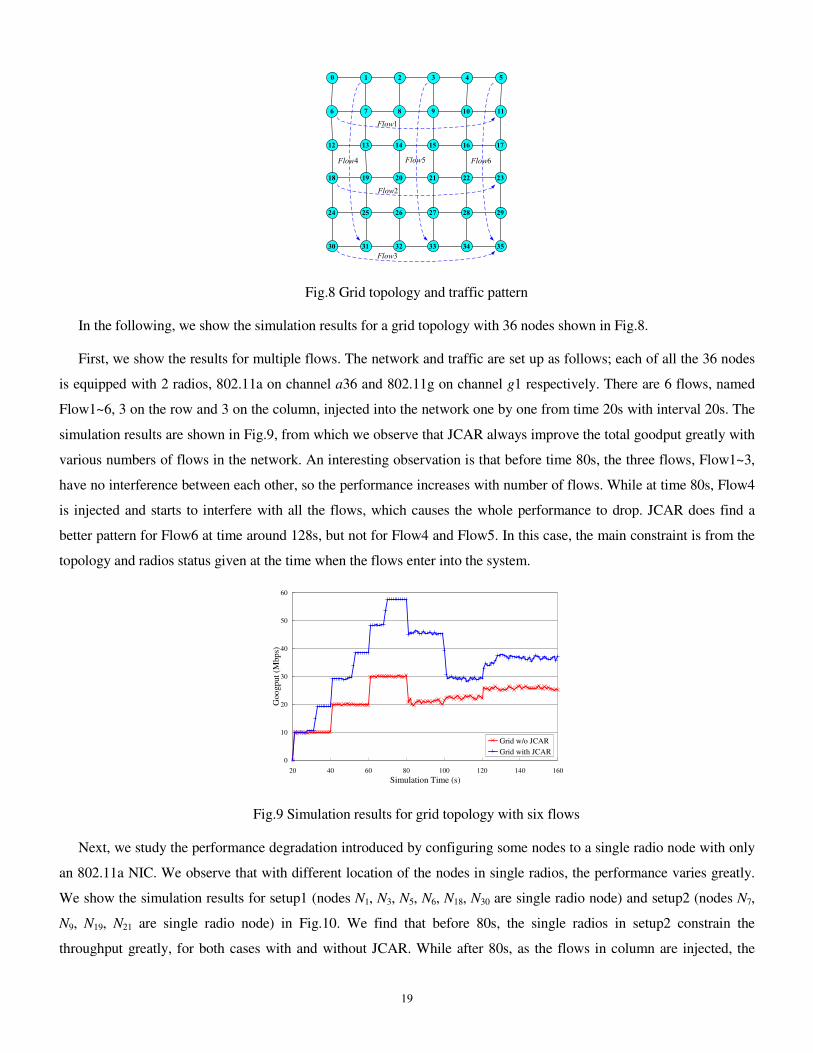
Fig.8 Grid topology and traffic pattern

In the following, we show the simulation results for a grid topology with 36 nodes shown in Fig.8.

First, we show the results for multiple flows. The network and traffic are set up as follows; each of all the 36 nodes

is equipped with 2 radios, 802.11a on channel a36 and 802.11g on channel g1 respectively. There are 6 flows, named

Flow1~6, 3 on the row and 3 on the column, injected into the network one by one from time 20s with interval 20s. The

simulation results are shown in Fig.9, from which we observe that JCAR always improve the total goodput greatly with

various numbers of flows in the network. An interesting observation is that before time 80s, the three flows, Flow1~3,

have no interference between each other, so the performance increases with number of flows. While at time 80s, Flow4

is injected and starts to interfere with all the flows, which causes the whole performance to drop. JCAR does find a

better pattern for Flow6 at time around 128s, but not for Flow4 and Flow5. In this case, the main constraint is from the

topology and radios status given at the time when the flows enter into the system.

0

10

20

30

40

50

60

20 40 60 80 100 120 140 160

Simulation Time (s)

Goo

gp

ut

(Mbp

s)

Grid w/o JCAR

Grid with JCAR

Fig.9 Simulation results for grid topology with six flows

Next, we study the performance degradation introduced by configuring some nodes to a single radio node with only

an 802.11a NIC. We observe that with different location of the nodes in single radios, the performance varies greatly.

We show the simulation results for setup1 (nodes N1, N3, N5, N6, N18, N30 are single radio node) and setup2 (nodes N7,

N9, N19, N21 are single radio node) in Fig.10. We find that before 80s, the single radios in setup2 constrain the

throughput greatly, for both cases with and without JCAR. While after 80s, as the flows in column are injected, the

20

throughput drops greatly due to interference. Note JCAR in setup2 successfully adjusts CA and routing for Flow3 at

time around 68s and Flow6 at time around 128s, which lie in the border and are not affected by the single radio in the

middle.

0

10

20

30

40

50

60

20 40 60 80 100 120 140 160

Simulation Time (s)

Goodp

ut

(Mbps)

Setup1 w/o JCAR

Setup1 JCAR

Setup2 w/o JCAR

Setup2 JCAR

Fig.10 Simulation results for grid topology with single radio nodes

Therefore, the performance improvement of JCAR is high but the improvement factor is determined by the network

topology, traffic pattern, and the nodes with single radios. To further evaluate the performance of our JCAR, we carry

out the simulation in a random topology. We randomly generate a topology with 30 nodes with the space geography

same as that in Grid topology. 5 random connections are set up for 5 random node pairs. Two types of nodes are in the

network: single radio node with only 802.11a, and multi-radio node with both 802.11a and 802.11g. The percentage of

number of multi-radio nodes in the random network is varied for 50%, 75% and 100% respectively, and we show the

average results from 10runs. From Fig.11, we observe that JCAR improves the throughput performance consistently for

different percentage of number of multi-radio nodes in the network.

0

2

4

6

8

10

12

14

16

50% 75% 100%

Percentage of multi-radio node

Goo

dp

ut

(Mb

ps)

w/o JCAR

JCAR

Fig.11 Simulation results for random topology

B. Experiemental Results

We also evaluate the performance of JCAR in a more realistic scenario, i.e., a 9-node wireless testbed. All the nodes

in the testbed locate on one floor in the east wing of our office building with floor-to-ceiling walls and glass or solid

21

wood doors. We place the nodes in offices, lounge, aisle, and labs. We deliberately place the nodes in a crossover like

topology and prevent the two-hop away devices from hearing each other1. See Fig. 12 for the locations of all the nodes.

29

21

11

18

24

31

27

10

28

N

Approx. 60 m

Appro

x.

50 m

Fig. 12 Topology of the wireless testbed.

All 9 nodes are DELL OPTIPLEX GX260/270/280 desktop PCs with Pentium III or IV processors. They all run

Windows XP with TCP SACK option enabled. Among these nodes, nodes 10, 24, 27, 28, and 31 are equipped with two

802.11a/b/g combo cards. Each of the remaining nodes has a single 802.11 a/b/g card. We use three types of wireless

cards in the testbed: Proxim ORiNOCO 11 a/b/g Gold PCI cards, LINKSYS Dual-Band Wireless A+G adapters, and

CISCO Aironet 802.11 a/b/g Wireless Adapters.

In Fig. 12, the dash link between two nodes represents an 802.11a link, and the solid link indicates an 802.11g link.

We find that not all the wireless adapters are able to operate in 802.11g 54Mbps ad hoc mode, maybe because

supporting 54Mbps in ad hoc mode is not mandatory according to IEEE 802.11 standard. Therefore the actually

bandwidth can be achieved in 802.11g ad hoc mode is vendor specific [33]. In order to test JCAR with more potential

candidate patterns when the link capacity is comparable, we intentionally force 802.11a/g card to work at lower data

rate, i.e. 11(for 11b)/12(for 11a) Mbps. We have conducted a series of TCP throughput tests on each wireless link to

ensure that all links indeed work around 11Mbps data rate. In addition, RTS/CTS handshake is disabled during the

experiments.

B.1 Channel switching overhead

We first evaluate the overhead introduced by channel switching to TCP protocol. We setup a three-hop TCP

connection from node 31 to node 11 and let the TCP flow traverse along the route g(1)->a(36)->g(1), where g(1)

denotes the TCP flow using the wireless card operating in 802.11g mode, channel 1 to transmit the data. The TCP

throughput measured at node 11 is shown in Fig.13, where the time interval between any two consecutive points is

1 In this setup, some two-hop away devices can occasionally hear the broadcasting packets from each other, but the signal quality between them

are not of sufficient quality to support sustainable TCP transmission.

22

about 0.5s. We start the TCP connection at time 0 and enable JCAR around 12s. We observe the channel switching

action is triggered at 14s. The wireless NIC card is instructed to switch to channel g(11). It takes about 100~200ms for

the wireless NIC card to finish the channel switching action (and possible some re-synchronization action defined by

802.11 MAC). The TCP throughput falls down at 14th second and recovers at 15

th second. Due to increased channel

diversity, the TCP flow achieves almost doubled throughput after 16s. From this experiment, we observe that JCAR can

improve the performance of TCP greatly, while the overhead introduced to TCP connection is very small even it

traverses 3 hops.

0.0

0.5

1.0

1.5

2.0

2.5

3.0

3.5

4.0

4.5

5 10 15 20

Time (s)

Thro

ug

hput

(Mbps)

TCP

Fig. 13 Impact of channel switching to TCP

B.2 TCP throughput comparison

We compare the performance between the fixed channel assignment scheme and the JCAR solution when two TCP

flows are running from node 29 to 11 and from node 18 to 21, respectively. For the fixed channel assignment scheme,

we allocate channel 36 to all the 11a cards and channel 6 to the 11g cards. We use WCETT routing, which, to our

knowledge, is the best available routing protocol designed for multi-radio multi-hop wireless networks [5]. The

experiments are conducted in mid-night to minimize the interference from other 802.11b WLANs deployed in the

building.

When just one TCP flow, either from node 29 to 11 or from node 18 to 21 (denoted as Flow 29->11 and Flow 18-

>21, respectively), traverses the testbed, we find that for the fixed channel assignment scheme, the best route for the

TCP flow from node 29 to 11 is a(36)->a(36)->g(6)->g(6) or a(36)->g(6)->g(6)->a(36). Since the throughputs of the

above two cases are close, we only show the result of the first one in Fig. 14. When route is chosen as a(36)->g(6)-

>a(36)->g(6), the performance is worse than the previous cases since here the wireless link between node 24 and 10

becomes a hidden link of the link between node 29 and 31 since the transmission of 24->10 can not be sensed by node

29. Similarly, link 10->11 is hidden from node 31.

23

Under JCAR, no matter what the initial routes the scheme chooses, the algorithm will converge to a diversified

channel assignment, e.g., a(36)->g(6)->a(40)->g(1). Since all four channels allocated to the four wireless links are

orthogonal, the throughput of Flow 29->11 is maximized.

Similar phenomena can be found for Flow 18->21. Note that the throughput of Flow 18->21 is a little bit lower than

that of Flow 29->11. This is because the path from 18 to 21 needs to traverse more floor-to-ceiling walls than that from

29 to11. We can see from Fig. 12 that nodes 24, 10, and 11 are placed in the same corridor. Therefore the signal

attenuation along the path from 18 to 21 is more severe than that from 29 to 11.

One flow TCP performance

0.0

1.0

2.0

3.0

4.0

Flow 29->11 Flow 18->21

Th

rou

ghp

ut

(Mbp

s)

Fixed CA

JCAR

Fig. 14 One flow TCP performance comparison.

29 31 24 10 11

18

27

28

21

a(36)

a(36)

a(36)

a(36)

g(6)

g(6)g(6)

g(6)

29 31 24 10 11

18

27

28

21

a(36)

g(6)

a(44)

g(6)

g(11)

g(1)a(40)

a(40)

Solution for Fixed CA Solution for JCAR

Fig 15. The solution for fixed CA and JCAR in crossover TCP flows case.

Fig. 14 shows the TCP throughput comparison between the fixed channel assignment scheme (denoted as Fixed CA)

and the proposed JCAR solution. We can see that JCAR can provide up to 100% performance improvement over the

fixed CA for both flows. Fig 15 shows the channel assignment and routing solution of the two schemes when Flow 29-

>11 and Flow 18->21 traverse the testbed simultaneously.

In this case, the path for the fixed CA scheme is chosen based upon similar reason mentioned in the one flow case.

For JCAR, although channel 6 of 11g and channel 40 of 11a have to be re-used by the four links around node 24, the

channels of the wireless links at the edge of the testbed are diversified. Therefore JCAR still can provide up to 53%

performance gain (See Fig. 16).

24

Crossover flows TCP performance

0.0

0.4

0.8

1.2

1.6

2.0

Flow 29->11 Flow 18->21

Th

rou

gh

pu

t (M

bp

s)

Fixed CA

JCAR

Fig. 16 Crossover flows TCP performance comparison.

VII. RELATED WORK

To the best of our knowledge, we are not aware of any other work that provides a distributed solution by jointly

considering routing and channel assignment in multi-radio multi-channel multi-hop wireless networks with

heterogeneous radios. But various previous studies have addressed some relevant aspects of the problem.

For related theoretical work, routing has been jointly considered with scheduling or power control [15~17] in a

multi-hop wireless network. Motivated by the flexibility introduced by multi-radio and multi-channel, paper [18]

formalizes the problem for joint routing and channel switching in M3WNs with homogeneous radios and uses column

generation method to solve the problem. However, all these work focus on the problem of joint routing and channel

scheduling assuming a perfect MAC, and does not take interference/collisions into consideration in the formation while

JCAR does. A centralized routing and channel assignment algorithm which iteratively uses routing and channel

assignment is proposed in [19] for multi-channel and multiple homogeneous radios, where their simulation results

demonstrate some performance improvement. However, again collision is not considered. Recent work [34] analyzes

the asymptotic bound of the throughput capacity and concludes that it is dependent only on the ratio of the number of

channels to the number of radios per node. Joint routing and scheduling by perfect MAC with multi-channel and multi-

radio are formulated in [35] and [36], where a constant factor approximation and an achievable low bound are proposed

respectively. From those theoretical works, however, it is not able to derive distributed algorithms straightforwardly

because of the perfect MAC assumption and real time information exchange overhead.

For distributed algorithms, most of related works focus on CA or routing separately. For channel assignment, papers

[20-22] are targeting at a MAC layer solution and hide the channel diversity to routing and upper layer protocols.

Currently IEEE standard [1] only defines the MAC protocol for single channel. Papers [22-25] propose an extension

based on dynamic channel selection and switching at packet level with the requirement that the NICs provide carrier

sense simultaneously at all channels, or multiple NICs work coordinately at packet level (e.g., exchange handshaking

packets on one NIC, and data packet transmissions followed at the other NIC).

25

For routing algorithms, paper [4] proposes a link quality aware routing protocol for multi-hop wireless networks,

and paper [5] proposes a routing metric called WCETT, which considers expected packet transmission time and

channel diversity for a path. To the best of our knowledge, the routing in [5] is most up-to-date system work addressing

the routing in M3WNs. However, it assumes the channel has been configured by other protocols and only focuses on

routing.

There are several works considering both CA and routing, but no jointly as done in this paper. Paper [26] provides a

combined solution consisting of channel assignment and routing by assuming each node has enough number of

homogeneous radios and assigns some of the radios fixed on certain channel only for receiving. Besides that we

consider jointly CA and routing, another difference from the work [26] is that we consider heterogeneous radios and

does not require each node in the network equipped more than one homogenous radio. Both papers [28] and [29]

propose a mesh based framework for routing and channel assignment, where the focused mesh has access points (AP)

connected by a wired network. The difference of the two papers is that paper [28] chooses to solve the AP selection

problem for a single radio case, while paper [29] proposes a channel assignment solution by categorizing multi-radios

into uplink and downlink radios, and proposes a load balanced routing to AP. Unfortunately, the two solutions can only

be used in a wireless network whose topology is a tree based structure.

Therefore, none of the related work jointly considers routing and channel assignment for a M3WN with one or more

heterogeneous commercial standardized radios on each node. In addition, the analysis of the hidden traffic and explicit

interference consideration also differentiates our work with others.

VIII. CONCLUSIONS

In this paper, we discuss how to improve the performance by joint channel assignment and routing for a

heterogeneous multi-radio multi-channel multi-hop wireless network. Targeting at developing a distributed algorithm,

we first present CCM as a critical metric that quantifies the difference for various JCAR patterns in terms of air time

cost due to collisions. The basic idea of our distributed JCAR algorithm is to select a JCAR pattern that results in

smallest metric at each node locally, where both the feasibility and connectivity are guaranteed in the algorithm. We

propose a novel software solution, called Layer 2.5 CA, which resides between the 802.11 MAC layer and routing layer

to coordinate – in a distributed fashion and without resorting to tight clock synchronization – the channel assignment

and routing among neighboring nodes in a multi-hop wireless network. We built a multi-hop wireless network testbed

with 9 wireless nodes, each equipped with multiple 802.11 a/b/g combo cards. Through extensive simulations using the

network simulator NS2 and experimental testing on the testbed, we have demonstrated the efficacy of our proposed

software solution. We plan to expand our testbed and perform more extensive testing. In addition, we plan to further

explore several design issues (e.g., chain puzzle, mobility, etc) and improve the performance and efficiency of our

protocol on channel switching.

26

ACKNOWLEDGEMENT

We thank our colleagues Yongqiang Xiong and Yunxin Liu for help on building the experiment testbed. And we

think R. Draves and his group for their work on MCL and we use it in our testbed for routing support.

REFERENCES

[1] IEEE standard for Wireless LAN Medium Access Control (MAC) and Physical Layer (PHY) specifications, ISO/IEC 8802-

11:1999(E), Aug. 1999.

[2] B.P. Crow and J.G. Kim. IEEE 802.11 Wireless Local Area Networks, IEEE Comm., Sept. 1997.

[3] S.Xu and T.Saadwi. Does the IEEE 802.11 MAC protocol work well in multihop wireless ad hoc networks. IEEE Comm.,

Jun. 2001.

[4] D.De Couto, D.Aguayo, J.Bicket, and R.Morris. High-throughput path metric for muli-hop wireless routing, In Mobicom,

2003.

[5] R.Draves, J.Padhye, and B.Zill. Routing in multi-radio, multi-hop wireless mesh networks, In Mobicom, 2004.

[6] G.Holland, N.Vaidya, and P.Bahl. A rate-adaptive MAC protocol for multi-hop rireless networks, Mobile Computing and

Networking, 2001.

[7] B.Sagdehi, V.Kanodia, A.Sabharwal, and E.knightly. Opportunistic media access for multirate ad hoc networks, in Mobicom

2002.

[8] J.Li, C.Blake, D.De Couto, H.Lee, and R.Morris. Capacity of ad hoc wireless networks, In Mobicom 2001.

[9] H.Wu, Y.Pong, et al. Performance of Reliable Transport Protocol over IEEE 802.11 Wireless LAN: Analysis and

Enhancement. In INFOCOM 2002.

[10] G.Bianchi. Performance Analysis of the IEEE 802.11 Distributed Coordination Function. IEEE Journal on Selected Area in

Comm., V18, N3, March 2000.

[11] M.M.Carvalho and J.J.Garcia-Luna-Aceves. A scalable model for channel access protocols in multihop ad hoc networks, In

Mobicom’04, Sept. 2004.

[12] F.Alizadeh-Shabdiz and S.Subramaniam. Analytical models for single-hop and multi-hop ad hoc networks,

BROADNETS'04, Oct. 2004.

[13] “NS”, URL http://www-mash.cs.berkeley.edu/ns/.

[14] D.B.Johnson, D.A.Maltz, and Y.Hu. The Dynamic Source Routing protocol for mobile ad hoc networks (DSR). Internet draft,

April 2003. http://www.ietf.org/ internet-drafts/draft-ietf-manet-dsr-09.txt

[15] R.L.Cruz and A.V.Santhanam, Optimal routing, link scheduling and power control in multi-hop wireless networks, Proc.

IEEE INFOCOM'03, 2003

[16] K.Jain, J.Padhye, V.N.Padmanabhan and L.Qiu, Impact of interference on multi-hop wireless network performance, Proc.

IEEE MobiCom'03, 2003.

[17] M.Kodialam and T.Nandagopal, Characterizing achievable rates in multi-hop wireless networks: the joint routing and

scheduling problem Proc. IEEE MobiCom'03, 2003.

[18] J.Zhang, H.Wu, Q.Zhang, B.Li, Joint Routing and Scheduling in Multi-radio Multi-channel Multi-hop Wireless Networks,

Broadnets’05, 2005.

[19] A. Raniwala, K. Gopalan and T. Chiueh, Centralized channel assignment and routing algorithms for multi-channel wireless

mesh networks, ACM MC2R, vol. 8, no. 2, April 2004.

[20] C.Chang, P.Huang, C.Chang and Y.Chen, Dynamic Channel Assignment and Reassignment for Exploiting Channel Reuse

Opportunities in Ad hoc Wireless Networks. IEICE Trans.Commun., Vol.E86-B, No.4, April 2003

[21] P.Bahl, R.Chandra and J.Dunagan, SSCH: Slotted seeded channel hopping for capacity improvement in IEEE 802.11 ad hoc

wireless networks, Proc. IEEE MobiCom'04, 2004.

27

[22] J.So and N.H.Vaidya, Multi-channel MAC for ad hoc networks: Handling multi-channel hidden terminals using a single

transceiver. Proc. MOBIHOC’04, 2004.

[23] S.Wu, C.Lin, Y.Tseng and J.Sheu, A new multi-channel MAC protocol with on-demand channel assignment for multi-hop

mobile ad hoc networks, Proc. I-SPAN’00, 2000.

[24] N.Jain and S.Das, A multichannel CSMA MAC protocol with receiver-based channel seletion for multihop wireless

networks, Proc. IC3N01, 2001

[25] A.Nasipuri and S.R.Das, Multichannel CSMA with signal power-based channel selection for multihop wireless networks,

Proc. VTC’00, 2000.

[26] P.Bahl, A.Adya, J.Padhye, A.Wolman, Reconsidering Wireless Systems with Multiple Radios. ACM CCR, Jul 2004.

[27] J.So, N.H.Vaidya, A Routing Protocol for Utilizing Multiple Channel in Multi-Hop Wireless Networks with a Single

Transceiver, TR.Oct.2004

[28] J.So, N.H.Vaidya, Routing and Channel Assignment in Multi-Channel Multi-hop Wireless Networks with Single-NIC

Devices, TR. Dec.2004

[29] P.Kyasanur, N.H.Vaidya, Routing in Multi-Channel Multi-Interface Ad hoc Wireless Networks, TR.Dec.2004

[30] A. Raniwala, and T. Chiueh, Architecture and Algorithms for an IEEE 802.11-Based Multi-channel Wireless Mesh Network,

Infocom’05, 2005.

[31] H.Wu, X. Wang, Y. Liu, Q. Zhang, and Z. Zhang, SoftMAC: Layer 2.5 MAC for VoIP Support in Multi-hop Wireless

Networks, IEEE Secon’05, Sept. 2005

[32] Microsoft Mesh Connectivity Layer (MCL) Software, http://research.microsoft.com/mesh.

[33] ---, Ad-hoc wireless connections limited to 11mbps, available at: http://labs.pcw.co.uk/2005/03/adhoc_wireless_.html, Mar.

2005.

[34] P. Kyasanur and N. Vaidya, Capacity of multi-channel wireless networks: impact of number of channels and interfaces, Proc.

IEEE MobiCom'05, 2005

[35] M. Alicherry, R. Bhatia and L. Li, Joint channel assignment and routing for throughput optimization in multi-radio wireless

mesh networks, Proc. IEEE MobiCom’05, 2005.

[36] M. Kodialam and T. Nandagopal, Characterizing the capacity region in multi-Radio, multi-Channel wireless mesh networks,

Proc. IEEE MobiCom'05, 2005.

[37] A. Rao,I. Stoica, An Overlay MAC Layer for 802.11 Networks, Proc. Mobisys 2005.

28

Appendix A

Estimation of the collision probablity on a link

A B H

Fig.A.1 Scenario for hidden terminal

CSMA/CA is used in the current 802.11 MAC and will also be used in future UWB MAC as a contention based

access method. It provides satisfactory collision avoidance if the interfering transmitters could sense each other.

Therefore, majority wireless collisions in multi-hop wireless networks are due to the hidden terminal effect [3]. The

classical hidden terminal scenario is shown in Fig.A.1, where node H can not sense the transmission from node A to B.

When node H starts a transmission, it may cause collision at node B, and therefore node H is called a hidden terminal to

node A. In the following discussion, for simplicity, we only focus on the collisions caused by hidden terminals, and

ignore the collisions caused by contention nodes within the range of carrier sense since the chance for the latter to occur

is much smaller than that caused by hidden terminals in a multi-hop scenario.

A B

M1 N1

M3

N3

M2N2

Fig.A.2 Scenario for hidden links

If an interfering link that contains hidden terminals to the data transmission on a given link, this interfering link is

called as a hidden link of the given link. For example, in Fig.A.2, links from node Mx to Nx (x=1,2,3) containing hidden

terminals (node in the shadowed area) to the transmission on link from node A to B, ( l

BAL ),(), are hidden links of link

l

BAL ),(. We categorize the hidden links by the location of the interfering nodes (hidden terminals) into three cases:

hidden link, co-hidden link and full-hidden link. The three classes of hidden links are shown in Fig.3, and are discussed

below.

Case 1: we consider link l

NML ),( 11

, where only the data transmission from source node M1 is interfering with the

reception of link l

BAL ),( at node B. In this case, link l

NML ),( 11

is a hidden link of link l

BAL ),(. Case 2: we consider link

l

NML )2,2(, where only the ACK transmission to destination node N2 is interfering with link l

BAL ),(. Note that link l

NML ),( 11

29

and link l

NML ),( 22

are symmetric, therefore we say link l

NML ),( 22

is a co-hidden link of link l

BAL ),(. Case 3: for link l

NML ),( 33

,

both data and ACK transmissions are interfering with link l

BAL ),(. We refer link l

NML ),( 33

as a full hidden link of link

l

BAL ),(. For convenience, we use )( ),(

l

BAx LH to denote the hidden link case x (x=1,2,3) observed at link l

BAL ),(.

As discussed before, to compute the collision probability, we only need to consider traffic on these hidden links

since they contribute most to the collisions observed at link l

jiL ),(. We assume that the traffic pattern on all interfering

links follows Poisson arrival. So the collision probability is given by

])([)( )(

]})([)( )(exp{1

)(

,

),(),(

,

),(

,

),(),(

)(

,

),(

,

),(),(

)(

,

),(

,

),(),(

)(

,

),(),(

,

),(

,

),(),(

)(

,

),(

,

),(),(

)(

,

),(

,

),(),(),(

),(3),(),(2),(),(1),(

),(3),(),(2),(),(1),(

∑∑∑

∑∑∑

∈∈∈

∈∈∈

++++++≈

++−+−+−−=

lji

lnm

lji

lnm

lji

lnm

lji

lnm

lji

lnm

lji

lnm

LHL

ACKl

nm

l

nm

DATAl

nm

DATAl

ji

l

nm

LHL

ACKl

nm

DATAl

ji

l

nm

LHL

DATAl

nm

DATAl

ji

l

nm

LHL

ACKl

nm

l

nm

DATAl

nm

DATAl

ji

l

nm

LHL

ACKl

nm

DATAl

ji

l

nm

LHL

DATAl

nm

DATAl

ji

l

nm

l

ji

TrTTTTrTT

TrTTTTrTTp

λλ

λλ

,

where DATAl

jiT,

),( and ACKl

jiT,

),( denote the transmission time of one DATA frame and one MAC ACK frame on link l

jiL ),(,

respectively.

Therefore, if we have the traffic information l

jir ),( and channel status on each link, we can estimate the collision

probability recursively by assuming the hidden links for any link are known (which is reasonable as these hidden links

are determined by the node locations).

Appendix B Algorithm to check network connectivity

Before, we describe the algorithm, we first introduce some notation. For node i, the set of its neighbor nodes on

channel l is denoted as l

iN , then the whole set of neighbor nodes of node i is Ul

l

ii NN = . We further divide Ni into two

classes, denoted by Ni,s and Ni,m, respectively, where Ni,s consists of all nodes connecting to node i using exact one

channel, and Ni,m= Ni- Ni,s. Further, let l

siN , denote the set of all single radio neighbors of node i on channel l.

l

si

l

i

l

mi NNN ,, −= denotes the multi-radio neighbors of node i, but each of them has at least one connection to node i (i.e.,

the connection on channel l).

Next we would like point out one interesting and critical phenomena in checking whether the connectivity can be

maintained under a new JCAR pattern. As shown in Fig.4, to keep connectivity, a neighbor node Ul

sj

l

si NNk ,,∈ (that has

single channel connectivity with node i or j on channel l), must also switch channel with node i and j. However, if node

k further has its single channel neighbor q on l that is not a neighbor node of node i or j, i.e., }0{,,, ≠− Ul

si

l

sj

l

sk NNN , then

the connectivity of nodes k and q will break if q does not switch with k. In the above example, node i should give up the

channel switching with node j. Note here even for a neighbor with multiple radios, it may still have the chain puzzle

problem. For example, node k’ is a multi-radio neighbor of node i or j, where a dashed line denotes the case when there

30

is another connection between j and k’ in Fig.4. If node k’ has single channel connectivity on l with any

node Ul

sj

l

si NNk ,,∈ , then we also needs to check whether k’ contains chain puzzle since it needs to switch channel to

maintain the connectivity with k. We summarize the connectivity maintenance procedures, in pseudo codes, in Fig.A.3.

The algorithm returns either a set of nodes that will switch with nodes i and j, the set Q, or indicates that the switch is

denied.

}

;return

}FALSE;{return })0{( If

each For

}Scan; togo };'{ {

)' AND ( If

ˆ'each For

:Scan

ˆ :Variable

}{}{ˆ

}{}{ˆ :Define

){,,(

,,,

,

,,

,,

,,,,

,,,,

Q

NNN

Qk

kQQ

NkQk

QNk

NQ

jiNNN

jiNNN

ljityConnectivi

l

si

l

sj

l

sk

l

sk

l

mji

l

sji

l

mi

l

mj

l

mji

l

si

l

sj

l

sji

7

6

5

4

3

2

1

≠−

∈

=

∈∈∃

−∈

=

−−=

−−=

U

U

U

U

Fig.A.3 Pseudo code for connectivity

Appendix C

Pseudo codes for the distributed JCAR algorithm

pattern each For

);,,( :selectionPattern

nodeeach For

channelfor JCAR trigger ,FWhen

pattern) JCARcurrent (the , :Variable

l

i

Pp

ljiPatternP

Nj

lTh

ppTH

l

i

H

cacheCAcache

∈

=

∈

>

==∆

3

2

1

};pattern new{deploy ) ( If

}; ;

{ ) ( If

; ,

cachecache

cachepcache

cachep

pii,pp

ppp

pp

CCMCCM

≠

=∆=∆

∆<∆

−=∆

7

6

5

4

31

}

next; goto )}0{( If

};}{{ )FALSE)(( If

each For

}ˆ :{set Pattern

ˆeach For

;least from by )}(ˆ{set channelSort

{ )FALSE),,(( If

:selectionpattern //CA

};0{''' :Variable

{ ),,(

ˆ

9

8

7

6

5

4

3

2

1

≠

−===

∈

→=

∈

∈=

≠

====

P

pPPpfeasiblity

Pp

llpatternP

Sl

FlCSlS

ljityConnectivi

PPPP

ljiPattern

l

i

t

};}{''{ )FALSE)(( If

'each For

} tofrom trafficmove :{''

) toousheterogene , and between ( channelFor

selectionpattern //routing:next

pPPpfeasiblity

Pp

l l PatternPP

ljil

−===

∈

=

14

13

12

11

10

U

;'''return

}

}; )'each out(For jump;''''{

)}0{( If

};}{{ )FALSE)(( If

each For

}' tofrom trafficmove and,' :{

'each For

;least from by )}('{set channelSort

{ )FALSE),,(( If

) toousheterogene , and between ( channeleach For

:selection routing andCA both with //pattern

'

U U

U

PPPP

SlPPP

P

pPPpfeasiblity

Pp

l l llPatternP

Sl

FlCSlS

ljityConnectivi

ljil

t

t

tt

t

t

l

i

=

∈=

≠

−===

∈

→=

∈

∈=

≠

26

25

24

23

22

21

20

19

18

17

16

15

Fig.A.4 Pseudo code for JCAR algorithm

Appendix D

Further refinement -- channel reconfiguration

In the example of section II, we observe that a newly constructed CA pattern is only suitable for traffic on certain

paths, and it may increase the possibility of chain puzzle since connectivity maintenance only guarantees there is at

least one channel between a node pair. When the channel utilization on channel l is fairly low, to make the CA more

diverse and more flexible for future traffic and to reduce the possibility of creating chain puzzle, we perform a

reconfiguration operation. The operation attempts to switch channel l to the one that has been used mostly in the

neighborhood of a node so that the connectivity for all node pairs within the two-hop range is increased.

The detailed procedure for channel reconfiguration is as follows, 1) when the utility of one channel is lower than a

certain threshold, it triggers the channel reconfiguration operation 2) for each neighbor node, it estimates the effect of a

32

channel switching for Ul

j

l

i NNQ = , and removes those patterns that result in network partition. 3) select l’ that is

supported by the interface, and l’ satisfies that *,'*, ll

i

ll

i FF < and δ−<+ H

ll

i

ll

i ThFF *,'*, . 4) if l’ exists, select the CA resulting

the largest connectivity, where a connectivity between any two nodes within the set of the two hop neighbors of both i

and j is counted by 1. Then the channel switching operation will be initiated.

Therefore, the distributed JCAR protocol should utilize certain diverse channel and routing pattern to improve the

performance of current system when the traffic load is high, and utilize as few as channels as possible to enlarge

connectivity between nodes when the traffic load is fairly light. Intuitively, utilizing a few common channels makes the

network topology flexible and reduces the possibility of chain puzzle in future patterns, which in turn gives more

choices for selecting new JCAR patterns. Thus, our distributed JCAR works as follows:

1) when the FAT on a channel is higher than ThH, trigger the distributed JCAR algorithm to search for new

patterns which may have a smaller CCM;

2) when the FAT on a channel is lower than ThL, trigger the procedure to reconfigure the channels for larger

connectivity.