distributed and stream data mining algorithms for frequent ... · distributed and stream data...
TRANSCRIPT
Universita Ca’ Foscari di Venezia
Dipartimento di InformaticaDottorato di Ricerca in Informatica
Ph.D. Thesis: TD-2006-4
Distributed and Stream Data MiningAlgorithms for Frequent Pattern Discovery
Claudio Silvestri
Supervisor
Prof. Salvatore Orlando
PhD Coordinator
Prof. Simonetta Balsamo
Author’s Web Page: http://www.dsi.unive.it/∼claudio
Author’s e-mail: [email protected]
Author’s address:
Dipartimento di InformaticaUniversita Ca’ Foscari di VeneziaVia Torino, 15530172 Venezia Mestre – Italiatel. +39 041 2348411fax. +39 041 2348419web: http://www.dsi.unive.it

To my wife

Abstract
The use of distributed systems is continuously spreading in several applicationsdomains. Extracting valuable knowledge from raw data produced by distributedparties, in order to produce a unified global model, may presents various challengesrelated to either the huge amount of managed data or their physical location andownership. In case data are continuously produced (stream) and their analysis isrequired to be performed in real time, communication costs and resource usage areissues that require careful attention in order to run computation in the optimallocation.
In this thesis, we examine in details the problems related to the Frequent PatternMining (FPM) in distributed and stream data and present a general framework foradapting an exact FPM algorithm to a distributed or streaming context. The FPMproblems we consider are Frequent Itemset Mining (FIM), and Frequent SequencesMining (FSM). In the first case, the input data are sets of items and the frequentpatterns are those included in a user-specified number of input set. The second oneconsists in finding frequent sequential patterns in a database of time-stamped events.Since the proposed framework uses (exact) frequent pattern mining algorithms asthe building block of the approximate distributed/stream algorithms, we will alsodescribe two efficient algorithms for FIM and FSM: DCI, introduced by Orlando etal., and CCSM, which is one of the original contributions of this thesis.
The resulting algorithms for distributed and stream FIM have been tested withreal world and synthetic datasets, and are able to find efficiently a good approxi-mation of the exact results and scale gracefully. The framework for FSM is almostidentical, but has not been tested yet. The few differences are highlighted in theconclusion chapter.

Sommario
La diffusione dei sistemi distribuiti e in continuo aumento in svariati campi applica-tivi e l’estrazione di correlazioni non evidenti nei dati grezzi prodotti puo esserestrategica per le organizzazioni coinvolte. Questo tipo di operazione e generalmentenon banale e, quando i dati sono distribuiti, presenta ulteriori difficolta legate siaalla mole di dati coinvolti che alla loro proprieta e locazione fisica. Nel caso i datisiano prodotti in flussi continui (stream) e sia necessario analizzarli in tempo reale,l’ottimizzazione dei costi di comunicazione e delle risorse necessarie sono aspetti chedebbono essere presi attentamente in considerazione.
In questa tesi sono analizzati in modo dettagliato i problemi legati alla ricercadi pattern frequenti (FPM) su dati distribuiti e stream di dati. In particolare epresentato un metodo generale per ottenere, a partire da un qualunque algoritmoesatto per FPM, un algoritmo approssimato per il FPM su dati distribuiti e streamdi dati. I tipi di pattern presi in considerazione sono gli itemset frequenti (FIM)e le sequenze frequenti (FSM). Nel primo caso i dati in ingresso sono insiemi dielementi (transazioni) ed i pattern frequenti sono a loro volta degli insiemi contenutialmeno in un numero di transazioni specificato dall’utente. Il secondo consiste invecenella ricerca di pattern sequenziali frequenti in una collezione di sequenze di eventiassociati a precisi istanti di tempo. Poiche il metodo proposto utilizza degli algoritmiesatti per l’estrazione di pattern frequenti come parti da riunire per ottenere deglialgoritmi per dati distribuiti e stream di dati, verranno anche descritti due algoritmiefficienti per FIM e FSM: DCI, presentato da Orlando ed altri, e CCSM, che e unodei contributi originali di questa tesi.
Gli algoritmi ottenuti applicando il metodo proposto sono stati utilizzati sia condati reali sia con dati sintetici per valutarne l’efficacia. Gli algoritmi per FIM sisono dimostrati scalabili ed in grado di estrarre efficientemente una buona approssi-mazione della soluzione esatta. Il modello per FSM e quasi identico, ma non eancora stato verificato sperimentalmente. Le poche differenze sono evidenziate nelcapitolo finale.

Acknowledgments
I would like to thank Prof. Salvatore Orlando for his guidance and support duringmy Ph.D. studies. I am also grateful to him for the opportunity to collaborate withthe ISTI-CNR High Performance Computing Lab. In this context, I would like tothank Raffaele Perego, Fabrizio Silvestri, and Claudio Lucchese who co-authoredsome of the papers I published and, in several ways, helped me in improving thequality of my work.
I thank my referees, Prof. Hillol Kargupta and Prof. Rosa Meo, for their atten-tion in reading this thesis and their valuable comments.
Most part of this work has been carried out at the Dipartimento di Informatica,Universita Ca’ Foscari di Venezia. I would like to thank all the faculty and personnelfor their support and for making the department a friendly place for doing research.Special thanks to Moreno and Matteo, for the long discussions on free software andother interesting subjects, and to all the others (ex-) Ph.D. students for the pleasanttime spent together: Chiara, Claudio, Damiano, Fabrizio, Francesco, Giulio, Marco,Matteo, Massimiliano, Ombretta, Paolo, Silvia, and Valentino.
In this last year I have been a guest at the Dipartimento di Informatica e Comu-nicazione, Universita degli Studi di Milano. I am grateful to Maria Luisa Damiani,for the opportunity of collaboration, and to the people working at the DB&SECLab, for the friendly working environment.
This work was partially supported by the PRIN’04 Research Project entitled”GeoPKDD - Geographic Privacy-aware Knowledge Discovery and Delivery”.
Finally, I would like to thank my extended family, who has never lost faith inthis long-term project, and all of my friends.

Contents
1 Introduction 11.1 Data distribution . . . . . . . . . . . . . . . . . . . . . . . . . . . . . 21.2 Data evolution . . . . . . . . . . . . . . . . . . . . . . . . . . . . . . 31.3 Applications . . . . . . . . . . . . . . . . . . . . . . . . . . . . . . . . 61.4 Association Rules Mining . . . . . . . . . . . . . . . . . . . . . . . . . 7
1.4.1 Frequent Itemsets Mining . . . . . . . . . . . . . . . . . . . . 91.4.2 Frequent Sequence Mining . . . . . . . . . . . . . . . . . . . . 101.4.3 Taxonomy of Algorithms . . . . . . . . . . . . . . . . . . . . . 11
1.5 Contributions . . . . . . . . . . . . . . . . . . . . . . . . . . . . . . . 131.6 Thesis overview . . . . . . . . . . . . . . . . . . . . . . . . . . . . . . 14
I First Part 17
2 Frequent Itemset Mining 192.1 The problem . . . . . . . . . . . . . . . . . . . . . . . . . . . . . . . . 20
2.1.1 Related works . . . . . . . . . . . . . . . . . . . . . . . . . . . 202.2 DCI . . . . . . . . . . . . . . . . . . . . . . . . . . . . . . . . . . . . . 21
2.2.1 Candidate generation . . . . . . . . . . . . . . . . . . . . . . . 222.2.2 Counting phase . . . . . . . . . . . . . . . . . . . . . . . . . . 222.2.3 Intersection phase . . . . . . . . . . . . . . . . . . . . . . . . . 24
2.3 Conclusions . . . . . . . . . . . . . . . . . . . . . . . . . . . . . . . . 25
3 Frequent Sequence Mining 273.1 Introduction . . . . . . . . . . . . . . . . . . . . . . . . . . . . . . . . 283.2 Sequential patterns mining . . . . . . . . . . . . . . . . . . . . . . . . 30
3.2.1 Problem statement . . . . . . . . . . . . . . . . . . . . . . . . 303.2.2 Apriori property and constraints . . . . . . . . . . . . . . . . . 323.2.3 Contiguous sequences . . . . . . . . . . . . . . . . . . . . . . . 323.2.4 Constraints enforcement . . . . . . . . . . . . . . . . . . . . . 33
3.3 GSP . . . . . . . . . . . . . . . . . . . . . . . . . . . . . . . . . . . . 343.3.1 Candidate generation . . . . . . . . . . . . . . . . . . . . . . . 343.3.2 Counting . . . . . . . . . . . . . . . . . . . . . . . . . . . . . . 35
3.4 SPADE . . . . . . . . . . . . . . . . . . . . . . . . . . . . . . . . . . . 353.4.1 Candidate generation . . . . . . . . . . . . . . . . . . . . . . . 353.4.2 Candidate support check . . . . . . . . . . . . . . . . . . . . . 363.4.3 cSPADE: managing constraints . . . . . . . . . . . . . . . . . . 37
ii Contents
3.5 CCSM . . . . . . . . . . . . . . . . . . . . . . . . . . . . . . . . . . . 373.5.1 Overview . . . . . . . . . . . . . . . . . . . . . . . . . . . . . 383.5.2 The CCSM algorithm . . . . . . . . . . . . . . . . . . . . . . . 383.5.3 Experimental evaluation . . . . . . . . . . . . . . . . . . . . . 43
3.6 Related works . . . . . . . . . . . . . . . . . . . . . . . . . . . . . . . 453.7 Conclusions . . . . . . . . . . . . . . . . . . . . . . . . . . . . . . . . 47
II Second Part 49
4 Distributed datasets 514.1 Introduction . . . . . . . . . . . . . . . . . . . . . . . . . . . . . . . . 51
4.1.1 Frequent itemset mining . . . . . . . . . . . . . . . . . . . . . 534.2 Approximated distributed frequent itemset mining . . . . . . . . . . . 53
4.2.1 Overview . . . . . . . . . . . . . . . . . . . . . . . . . . . . . 544.2.2 The Distributed Partition algorithm . . . . . . . . . . . . . . . 554.2.3 The APRed algorithm . . . . . . . . . . . . . . . . . . . . . . . 574.2.4 The APInterp algorithm . . . . . . . . . . . . . . . . . . . . . . 594.2.5 Experimental evaluation . . . . . . . . . . . . . . . . . . . . . 62
4.3 Conclusions . . . . . . . . . . . . . . . . . . . . . . . . . . . . . . . . 68
5 Streaming data 735.1 Streaming data . . . . . . . . . . . . . . . . . . . . . . . . . . . . . . 73
5.1.1 Issues . . . . . . . . . . . . . . . . . . . . . . . . . . . . . . . 745.2 Frequent items . . . . . . . . . . . . . . . . . . . . . . . . . . . . . . 74
5.2.1 Problem . . . . . . . . . . . . . . . . . . . . . . . . . . . . . . 755.2.2 Count-based algorithms . . . . . . . . . . . . . . . . . . . . . 755.2.3 Sketch-based algorithms . . . . . . . . . . . . . . . . . . . . . 81
5.3 Frequent itemsets . . . . . . . . . . . . . . . . . . . . . . . . . . . . . 825.3.1 Related work . . . . . . . . . . . . . . . . . . . . . . . . . . . 825.3.2 The APStream algorithm . . . . . . . . . . . . . . . . . . . . . 84
5.4 Conclusions . . . . . . . . . . . . . . . . . . . . . . . . . . . . . . . . 95
III 97
Conclusions 99
A Approximation assessment 103
Bibliography 107
List of Figures
1.1 Incremental data mining . . . . . . . . . . . . . . . . . . . . . . . . . 51.2 Data stream mining . . . . . . . . . . . . . . . . . . . . . . . . . . . . 61.3 Transaction dataset . . . . . . . . . . . . . . . . . . . . . . . . . . . . 91.4 Sequence dataset . . . . . . . . . . . . . . . . . . . . . . . . . . . . . 101.5 Effect of maxGap constraint . . . . . . . . . . . . . . . . . . . . . . . 121.6 Taxonomy of algorithms for frequent pattern mining . . . . . . . . . . 13
2.1 Set of itemsets compressed data structure . . . . . . . . . . . . . . . 232.2 Example of cache usage . . . . . . . . . . . . . . . . . . . . . . . . . . 25
3.1 GSP candidate generation . . . . . . . . . . . . . . . . . . . . . . . . 343.2 CCSM candidate generation . . . . . . . . . . . . . . . . . . . . . . . 403.3 Example of cache usage . . . . . . . . . . . . . . . . . . . . . . . . . . 413.4 CCSM idlist reuse . . . . . . . . . . . . . . . . . . . . . . . . . . . . . 423.5 Number of intersection for different intersection methods . . . . . . . 433.6 Number of frequent sequences in datasets CS11 and CS21 . . . . . . . 443.7 Execution times of CCSM and cSPADE- variable maxGap value . . . . 453.8 Execution times of CCSM and cSPADE- fixed maxGap value . . . . . 45
4.1 Similarity of APRed approximate results . . . . . . . . . . . . . . . . . 664.2 Number of spurious patterns as a function of the reduction factor r . 674.3 fpSim of the APInterp results . . . . . . . . . . . . . . . . . . . . . . . 684.4 Comparison of Distributed One-pass Partition vs. APInterp . . . . . . . 694.5 Speedup for two of the experimental datasets . . . . . . . . . . . . . . 70
5.1 Similarity and ASR as a func. of memory/transactions/hash entries . 955.2 Similarity and ASR as a function of stream length . . . . . . . . . . . 96C.3 Distributed stream mining framework . . . . . . . . . . . . . . . . . . 101

iv List of Figures
List of Tables
1.1 Taxonomy of data mining environments . . . . . . . . . . . . . . . . . 4
4.1 Datasets used in APRed experimental evaluation . . . . . . . . . . . . 634.2 Datasets used in APInterp experimental evaluation . . . . . . . . . . . 644.3 Test results for APRed . . . . . . . . . . . . . . . . . . . . . . . . . . . 654.4 Accuracy indicators for APInterp results . . . . . . . . . . . . . . . . . 71
5.1 Sample supports and reduction ratios . . . . . . . . . . . . . . . . . . 885.2 Datasets used in experimental evaluation . . . . . . . . . . . . . . . . 93

vi List of Tables
1Introduction
Data mining is, informally, the extraction of knowledge hidden in huge amounts ofdata. However, if we are interested in a more detailed definition, several differentones do exist [23]. Depending on the application domain (and on the author), Datamining could just mean the extraction of a particular aggregate information fromsomehow preprocessed data, or the whole process beginning with data cleaning andintegration, and ending with result visual representation. From now on, we willreserve the term Data mining to the first meaning, using the more general KDD(Knowledge Discover in Databases) for the whole workflow that is needed in orderto apply Data mining algorithms to real world problems.
The kind of knowledge we are interested in, together with the organization of in-put data and the criteria used to discriminate among useful and useless information,contributes to characterize a specific data mining problem and its possible algorith-mic solutions. Common data mining tasks are the classification of new objectsaccording to a scheme learned from examples, the partitioning of a set of objectsinto homogeneous subsets, the extraction of association rules and numerical rulesfrom a database.
In several interesting application frameworks, such as wireless network analysisand fraud detection, data are naturally distributed among several entities and/orevolve continuously. In all of the above-indicated data mining tasks, dealing witheither of these peculiarities provides additional challenges. In this thesis we will focuson the distribution and evolution issues related to the extraction of Association Rulesfrom transactional databases (ARM), one of the most important and common datamining task, both for the immediate applicability of the knowledge extracted by thiskind of analysis, and for the wide range of application fields where it can be used.Association Rules are rules relating the occurrence of distinct subset of items in thesame set, i.e. ”65 % of market basket containing steak and salad will also containswine”, or in the same collection of set ”50 % of customer that buy a CD playerwill, later, buy CDs”. In particular, we will concentrate our attention on the mostcomputationally expensive phase of ARM, the mining of frequent patterns fromdistributed and stream data. These patterns can be either frequent itemsets (FIM)or frequent sequences (FSM), i.e., respectively subsets contained in at least a userindicated number of input set and subsequence of at least a user specified number
2 1. Introduction
input sequences. Since we will use frequent pattern mining algorithms for static andnon-evolving datasets as the building block for our approximate algorithms, to beexploited on distributed and stream data, we will also describe efficient algorithmsfor FIM and FSM: DCI, introduced by Orlando et al. in [44], and CCSM, which isone of the original contributions of this thesis.
This chapter introduces, without focusing on any particular data mining task, thegeneral issues concerning the evolution of data, and their distribution/partitioningamong several entities. Then it quickly introduces ARM and its core FIM/FSMphase in centralized and non-evolving datasets. Both will be discussed more indetail both the first part of the thesis, since they constitute the foundation for thedistributed and streaming FIM/FSM problems. We also deal with taxonomy of bothFIM and FSM algorithms, which will be useful in understanding the reasons thatlead us to the choice of DCI and CCSM algorithms as the building blocks for ourdistributed and stream algorithms. The chapter concludes with a summary of theachievements of our research, and a description of the structure of the rest of thethesis.
1.1 Data distribution
Reasons leading to data distribution. In many real systems, data are naturallydistributed, usually due to a plural ownership or to a geographical distribution ofthe processes that produce the data. The logistic organization of entities involved inthe data collection process, performance and storage constraints, as well as privacyand company interest, may lead to the choice of using separate databases, insteadof a centralized one accessed by several remote locations.
The sales point of a large chain are a typical example: there is no need of acentral database for performing ordinary sale activities, and using it would makethe operations of the shop dependent on the reliability and bandwidth of the com-munication infrastructure. Gathering all data to a single site, after they have beenproduced, would be subject to the same ownership/privacy issues as using a cen-tralized database.
In other cases, data are produced locally in large volumes and immediately movedto other storage and analysis locations, due to the impossibility to store or processthem with the resources available at a single site, as in the case of satellite imageanalysis or high-energy physics experiments. In all of these cases, performing a datamining task means to coordinate the sites in a mix of partial movement of data andexchange of local knowledge, in order to get the required global model.
Homogeneous vs. heterogeneous data. Problems that are seemingly similarmay need sensibly different solutions, if considered in different communication anddata localization settings. Data can be either homogeneous or heterogeneous. If dataare represented by tuples, in the first case all data presents the same dimensions,
1.2. Data evolution 3
while in the second one data each node has its own schema. Let us consider twoexamples: the sales data of a chain of shops and the personal data collected about usby different department of public administration. Sales data contain a representationof the sale transactions and are maintained by the shop where the items were bought.In this case, data are homogeneous: data collected at different shop are similar, butrelated to different transactions. Personal data are also maintained at differentsite: the register office manages birth data, the tax register own tax data, anotherregister collect data about our cars. In this case, data are heterogeneous, since foreach individual each register maintains different kind of data.
Data localization is a key factor in characterizing data mining problems. Mostclassical data mining algorithms expect all data to be grouped in a unique datarepository. Each data mining task presents different issues when it is consideredin a distributed environment, instead of a centralized one. However it is possibleto identify a general requirement common to most distributed data mining systemarchitectures and tasks: careful attention should be paid to both communicationand computation resources, in order to use them in a nearly optimum way. Datadistribution issues and algorithms will be discussed in more details in chapter 4,with a focus on frequent pattern mining algorithms.
A good survey on distributed data mining algorithms and applications is [48].
1.2 Data evolution
In different application context, data mining can be applied either to past data,as a one time task, or repeatedly to evolving datasets. The classical data miningalgorithms refer to the first case: the full dataset is available and there will be nodata modification during the computation or between two consecutive computations.This is enough to understand a phenomenon and make plans for the future in mostcases.
In several applications, like wireless network analysis, intrusion detection, stockmarket analysis, sensor network data analysis, and, in general, any setting in whichevery information available should be used to make an immediate decision, the ap-proach based on finite statically stored data sets could be not satisfactory. Thesecases demands for new classes of algorithms, able to cope with evolutions of data.In particular, two issues need to be addressed: the complexity of recomputing ev-erything from scratch and the potential infiniteness of data. In case only the firstissue is present, the setting is referred to as Incremental/Evolving Data Mining ;otherwise, it is indicated as Stream Data Mining.
The presence and kind of data evolution is another key factor in characterizingdata mining problems.
4 1. Introduction
Data localization
Centralized A single entity can access every data
Distributed Each node can access just a part of the data and ...
homogeneous ... data related to the same entity (e.g.: people) areowned by just one node
heterogeneous ... data related to the same entity (e.g.: people) may bespread among several nodes
Data evolution
Statical Data are definitively stored and invariable (e.g.: relatedto some past and concluded event)
Incremental New data are inserted and access to past data is possible(e.g.: related to an ongoing event)
Evolving The dataset is modified with either updates, insertionsor deletions, and access to past data is possible.
Streaming Data arrives continuously and for an indefinite time. Ac-cess to past data is restricted to a limited to part of themor summaries.
Table 1.1: Taxonomy of data mining environments.
Incremental and Evolving Data Mining.
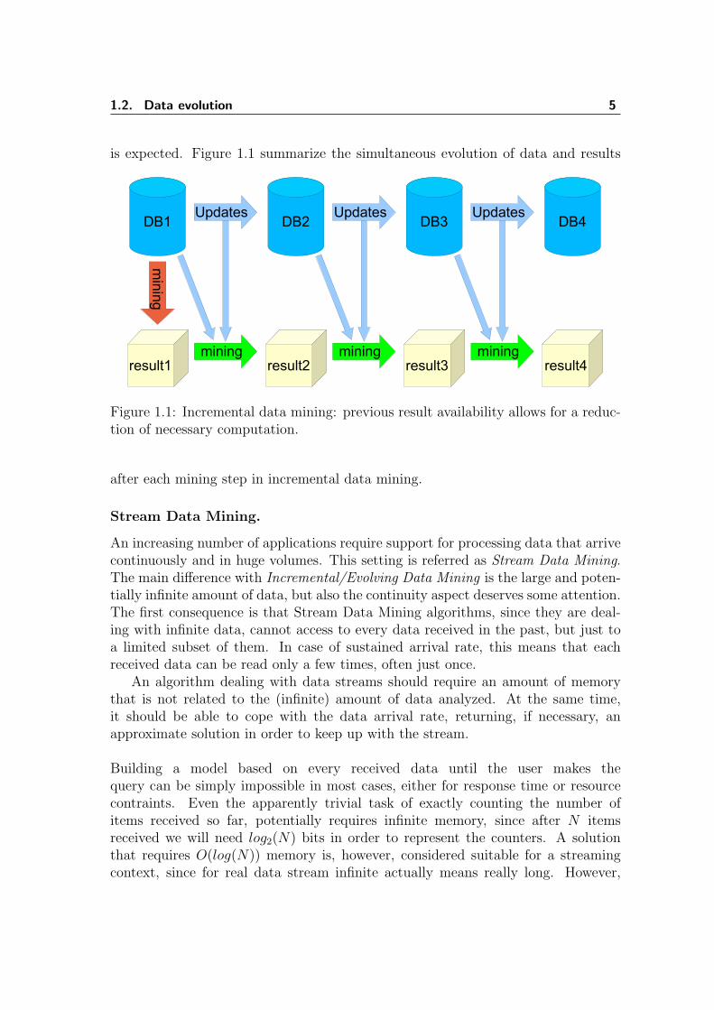
In incremental data mining, new data are repeatedly inserted into the dataset. Somealgorithm also take care of deletions or modifications of previous data, this case isindicated as evolving data mining. In a typical situation, we have a dataset D andthe results of the required data mining task on D. Then D is modified and thesystem is asked for a new result set. Obviously, a way to obtain the new result is torecompute everything from scratch, and it is possible since all past data are accessi-ble. However, this implies a computation time that in some case may clash with nearreal time system response requirements, whereas in other cases is just a waste of re-sources, especially when the dataset get bigger. Incremental/Evolving data miningalgorithms, instead, are able to update the solution according to dataset updates,modifying just the part of the result set that is interested by the modifications ofthe dataset. A fitting example could concern the sales data of a supermarket: at theend of each day, the daily update is performed. The overall amount of data is stillreasonable for an ordinary computation; however, there is no point in reprocessingsome year of past sales data. A better approach would be considering the past resultand the new data, and querying the past data only when a modification of the result
1.2. Data evolution 5
is expected. Figure 1.1 summarize the simultaneous evolution of data and results
Figure 1.1: Incremental data mining: previous result availability allows for a reduc-tion of necessary computation.
after each mining step in incremental data mining.
Stream Data Mining.
An increasing number of applications require support for processing data that arrivecontinuously and in huge volumes. This setting is referred as Stream Data Mining.The main difference with Incremental/Evolving Data Mining is the large and poten-tially infinite amount of data, but also the continuity aspect deserves some attention.The first consequence is that Stream Data Mining algorithms, since they are deal-ing with infinite data, cannot access to every data received in the past, but just toa limited subset of them. In case of sustained arrival rate, this means that eachreceived data can be read only a few times, often just once.
An algorithm dealing with data streams should require an amount of memorythat is not related to the (infinite) amount of data analyzed. At the same time,it should be able to cope with the data arrival rate, returning, if necessary, anapproximate solution in order to keep up with the stream.
Building a model based on every received data until the user makes thequery can be simply impossible in most cases, either for response time or resourcecontraints. Even the apparently trivial task of exactly counting the number ofitems received so far, potentially requires infinite memory, since after N itemsreceived we will need log2(N) bits in order to represent the counters. A solutionthat requires O(log(N)) memory is, however, considered suitable for a streamingcontext, since for real data stream infinite actually means really long. However,
6 1. Introduction
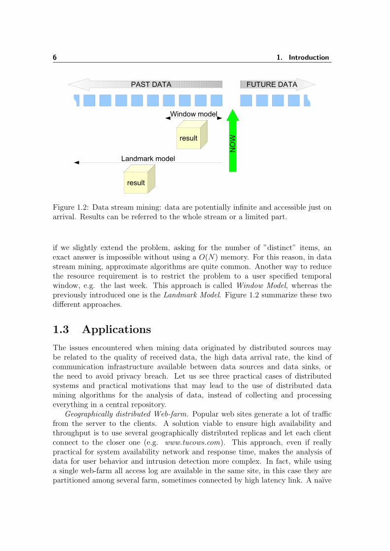
Figure 1.2: Data stream mining: data are potentially infinite and accessible just onarrival. Results can be referred to the whole stream or a limited part.
if we slightly extend the problem, asking for the number of ”distinct” items, anexact answer is impossible without using a O(N) memory. For this reason, in datastream mining, approximate algorithms are quite common. Another way to reducethe resource requirement is to restrict the problem to a user specified temporalwindow, e.g. the last week. This approach is called Window Model, whereas thepreviously introduced one is the Landmark Model. Figure 1.2 summarize these twodifferent approaches.
1.3 Applications
The issues encountered when mining data originated by distributed sources maybe related to the quality of received data, the high data arrival rate, the kind ofcommunication infrastructure available between data sources and data sinks, orthe need to avoid privacy breach. Let us see three practical cases of distributedsystems and practical motivations that may lead to the use of distributed datamining algorithms for the analysis of data, instead of collecting and processingeverything in a central repository.
Geographically distributed Web-farm. Popular web sites generate a lot of trafficfrom the server to the clients. A solution viable to ensure high availability andthroughput is to use several geographically distributed replicas and let each clientconnect to the closer one (e.g. www.tucows.com). This approach, even if reallypractical for system availability network and response time, makes the analysis ofdata for user behavior and intrusion detection more complex. In fact, while usinga single web-farm all access log are available in the same site, in this case they arepartitioned among several farm, sometimes connected by high latency link. A naıve
1.4. Association Rules Mining 7
solution is to collect all data in a centralized database, either periodically or in realtime, and it is in most case the best solution, at least if the data arrival rate is lowor we are not interested in recent data. However, this is not satisfying when logdata are huge, and real time analysis is required, as for intrusion detection.
Sensor network. The same kind of problems may arise, even worse, when thesources of data streams are sensors connected by a network. Quite often communi-cation link with sensors have a reduced bandwidth, for example in case of seismicsensors placed in inhabited places, far from computation infrastructures.
Financial network. Furthermore data centralization may be unfeasible whenconfidential information are handled and must not be shared with unauthorizedsubjects in order to protect privacy rights or company interests. A classical exampleconcerns the credit card fraud detection. Let us suppose that a group of banks isinterested in automatically detecting possible frauds; each participating entity isinterested in making the resulting model accurate, and based on as much data aspossible, but banks cannot communicate the transactions of their customers to otherbanks.
In all these cases, even if for different reasons, collecting all raw data to a repos-itory before analyzing them is unfeasible and distributed techniques are needed inorder to elaborate, at least partially, the data in place.
1.4 Association Rules Mining
As we have seen in the previous section, dealing with evolving and distributed datapresents several issues, independently of the particular targeted data mining task.However, each data mining task has its peculiarities, and the issues in different casesare not really the same, but just similar and related to the same aspect. In orderto analyze more thoroughly the issues and possible solutions, we have to focus on aparticular task or group of tasks. We have decided, in this thesis, to concentrate ourattention on Association Rules Mining, and more precisely on its most computa-tionally expensive phase, the mining of frequent patterns in distributed dataset anddata stream, where these patterns can be either itemsets (FIM) or sequences (FSM).
In this section we will quickly introduce the Association Rule Mining (ARM), oneof the most popular DM task [4, 18, 19, 54], both for the immediate applicability ofthe knowledge extracted by this kind of analysis and for the wide range of applicationfields where it can be applied, from medical symptoms developed in a patient toobjects sold in a commercial transaction.
Here our goal is just to quickly introduce this topic, and its computational chal-lenging Frequent Pattern Mining sub problem, by limiting our attention to thecentralized case. A more detailed description of the problem will be found in chap-ters 2 and 3 for the centralized sub problems, in chapter 4 for the distributed oneand in chapter 2 for the stream case.
8 1. Introduction
The essence of associative rules is the analysis of the co-occurrence of facts in acollection of set of facts. If, for instance, the data represent the objects bought inthe same shopping chart by the customers of a supermarket, then the goal will befinding rules relating the fact that a market basket contains an item with the factthat another item has been bought at the same time. One of these rules could be”people who buy item A also buy item C in conf% cases”, but also the more complex”people who buy item A and item B also buy item C in conf% cases” where conf%is the confidence of the rule, i.e. a measure of how much that rule can be trusted.Another interestingness measure, frequently used in conjunction with confidence, isthe support of a rule, which is defined as the number of records in the databasethat confirm the rule. Generally, the user specifies minimum thresholds for both, soan interesting rule should have both a high support and a high confidence, i.e. itshould be based on a significant number of cases to be useful, and at the same time,there should be few cases in which it is not valid.
The combined use of support and confidence is the measure of interestingnessmost commonly adopted in literature, but in some case can be misleading if the userdoes not look carefully at the big picture. Consider the following example: both Aand B appear in 80% of input data, and in 60% of cases, they appear in the sametransaction. The rule ”A implies B” has support 60% and confidence 60
80= 75%,
thus apparently this is a good rule. However, if we analyze the full context, we cansee that the confidence is lower than the support of B, hence the actual meaningof this rule is that A negatively influences B. The usage of other interestingnessmeasures has been widely discussed. However, there is no clear winner, and thechoice depends on the specific application field.
Sequential rules or (temporal association rules) are an extension of associationrules, which also considers sequential relationships. In this case, the input data aresequences of set of facts and the rules have to deals with both co-occurrences and”followed by” relationships. Continuing with the previous example about marketbasket analysis (MBA), this means considering each transaction as related to acustomer, identified by a fidelity card or something similar. So each input sequenceis the shopping history of a customer and a rule could be ”people who buy item Aand item B at the same time will also buy item C later in conf% cases” or ”peoplewho buy item A followed by item B within one week will also buy item C later inconf% cases”.
The extraction of both association rules and sequential rules from a database istypically composed of two phases. First, it is necessary to find the so-called frequentpatterns, i.e. patterns that occur in a significant number of records. Once suchpatterns are determined, the actual association rules can be derived in the formof logical implications: X ⇒ Y , which reads whenever X occurs in a transaction(sequence), most likely also Y will occur (later). The computationally intensive partis the determination of frequent patterns, more precisely of frequent itemsets forassociation rules and frequent sequences for sequential rules.
1.4. Association Rules Mining 9
1.4.1 Frequent Itemsets Mining
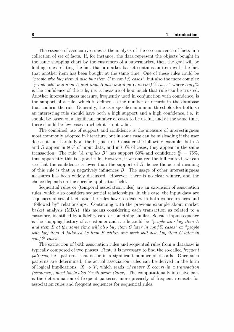
The Frequent Itemsets Mining (FIM ) problem consists in the discovery of subsetsthat are common at least to a user-defined number of input set. Figure 1.3 shows asmall dataset related to the previous MBA example. There are eight transactions,each containing a variable number of distinct items. If the user chosen minimumsupport is three, then the pair ”scanner and speaker” is a frequent pattern, whereas”scanner and telephone” is not a frequent one. Obviously, any larger pattern con-taining both a scanner and a telephone cannot be frequent. This fact is known asapriori principle and, expressed in a more formal way, states that a pattern can befrequent only if all its subsets are frequent too.
10/01/2002 12/02/2002 23/12/2002
10/11/200220/04/2002
16/05/2002 10/06/2002
Figure 1.3: Transaction dataset.
The computational complexity of the FIM problem derives from the exponentialsize of its search space P(M), i.e. the power set of M , where M is the set of itemscontained in the various transactions of a dataset D. In the example in Figure 1.3,there are 8 distinct items and the larger transaction contains four items, this lead to∑4
k=1
(8k
)= 162 possible patterns to examine, considering all transaction of maximal
length, and 48 considering the actual transaction lengths. However, the number ofdistinct patterns is 29 and the number of frequent pattern is even smaller, e.g., thereare just 7 items and 4 pairs occurring more than once, but only 4 items containedin more than two transactions.
Clearly, the naıve approach consisting in generating all subset for every transac-tion and updating a set of counters would be extremely inefficient. A way to prunethe search space is to consider only those patterns whose subsets are all frequent.The correctness of this approach derives from the apriori principle, which grantsthat it is impossible for discarded pattern to be frequent. The Apriori algorithm [6]and other derived algorithms [2, 9, 11, 25, 49, 50, 44, 55, 68] exactly exploits this
10 1. Introduction
pruning technique.
1.4.2 Frequent Sequence Mining
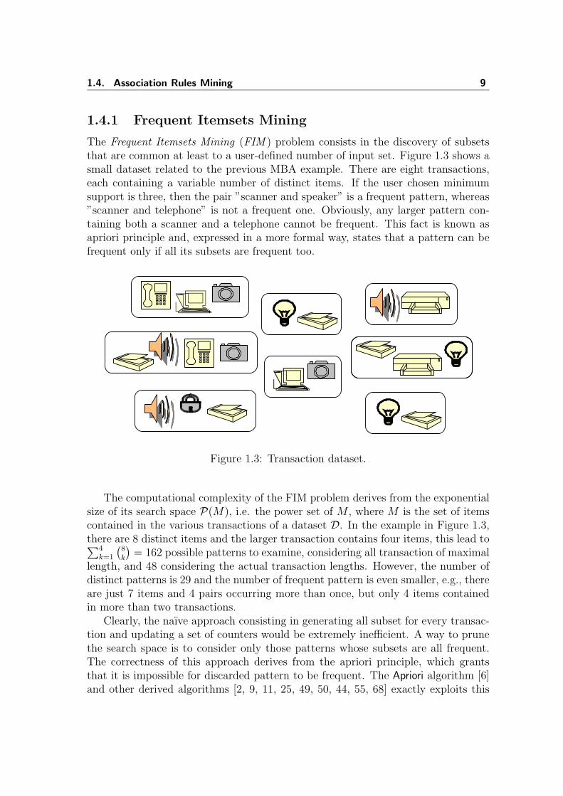
Sequential pattern mining (FSM) [7] represents an evolution of Frequent ItemsetsMining, allowing also for the discovery of before-after relationships between subsetsof input data. The patterns we are looking for are sequences of sets, indicating thatthe elements of a set occurred at the same time and before the elements containedin the following sets. The ”occurs after” relationship is indicated with an arrow,e.g. {A, B} → {B} indicates an occurrence of both item A and B followed by anoccurrence of item B. Clearly, the inclusion relationship is more complex than in caseof subsets, so it needs to be defined. Here we informally introduce this concept, whichwe will define formally in chapter 3. For now, we consider that a sequence pattern Zis supported by an input sequence IS, if Z can be obtained by removing items andsets from IS. As an example the input sequence {A, B} → {C} → {A} supports thesequential patterns {A, B}, {A} → {C}, {A} → {A}, but not the pattern {A, C},because the occurrence of A and C in the input sequence are not simultaneous.We highlight that the ”occurs after” relationship is satisfied by {A} → {A}, sinceanything between the two items can be removed.
Figure 1.4 shows a small dataset containing just three input sequences, each
10/01/2002 12/02/2002 23/12/2002
10/11/200220/04/2002
16/05/2002 10/06/2002
Figure 1.4: Sequence dataset.
associated with a customer according to the above example. For each transaction,
1.4. Association Rules Mining 11
the date is printed, but for the moment, we consider the time just a key for sortingtransactions. If we set the minimum support to 50%, we can see that the pat-tern ”computer and camera followed by a speaker” is frequent and supported bythe behavior of two customers. We observe that the apriori principle still holds forsequence patterns. If we define the containment relationship between patterns, anal-ogously to the one defined between patterns and input sequence, we can state thatevery subsequence of a frequent sequence is frequent. So we are sure that ”computerfollowed by a speaker” is a frequent pattern without looking at the dataset, becausethe above-mentioned pattern is frequent, and, at the same time, we know that everypattern containing a ”lamp” is not frequent.
The computational complexity of FSM is higher than that of FIM, due to thepossible repetitions of items within each pattern. Thus, having a small number ofdistinct items often does not help, unless the length of input sequences is small too.However, since the apriori principle is still valid, several efficient algorithms for FSMexist, based on the generation of frequent patterns from smaller frequent ones.
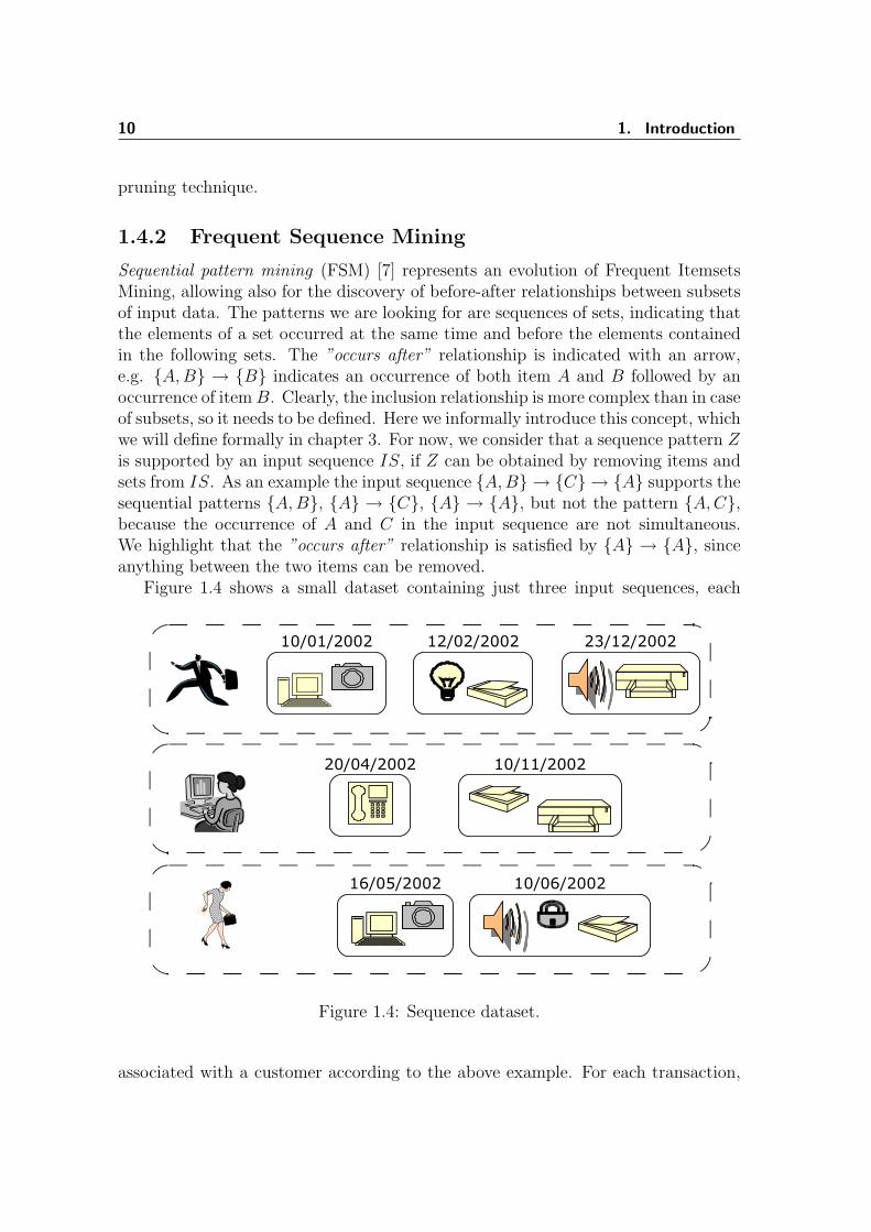
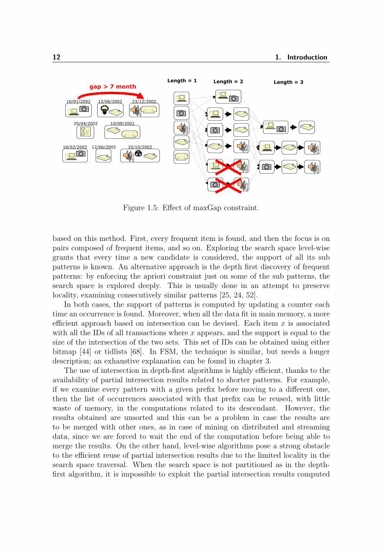
In several application context it is interesting to exploit the presence of a timedimension in order to obtain a more precise knowledge, and, in some case, to alsotransform an intractable problem into a tractable one by restricting our attentiononly to a the cases we are looking for. For example, if data represents the failurein a network infrastructure, when looking for congestion we are interested in shorttime periods, and the failure of an equipment a day after another one may be notas significant as the same sequence of failures within a few seconds. In this case,an expert of this domain can enforce a constraint on the maximum gap betweenoccurrences of events, thus obtaining a better focus on actually important patternsand a strong reduction in the complexity. In the example in Figure 1.4, if we decideto limit our research to occurrences having a maximum gap smaller than sevenmonth the pattern ”computer followed by a speaker” will be supported just by onecustomer shopping sequence, since in the first one the gap between the occurrenceof the computer and the occurrence of the speaker is too large.
Figure 1.5 shows the effect of maximum gap constraint on the support of someof the patterns of the above example: the deleted ones simply disappear, becausetheir occurrences have inadequate gaps. This behavior poses serious problems tosome of the most efficient algorithms, as we will explain in chapter 3, since some oftheir super-pattern may be frequent anyway. It is the case of the pattern ”camerafollowed by scanner followed by speaker” which has one occurrence with maximumgap equal to seven month even if ”camera followed by speaker” has no occurrenceat all.
1.4.3 Taxonomy of Algorithms
The apriori principle states that no superset of an infrequent set can be frequent.This determines a powerful pruning strategy that suggests a level-wise approach tosolve both FIM [4] and FSM [7] problems. Apriori is the first of a family of algorithms
12 1. Introduction
Figure 1.5: Effect of maxGap constraint.
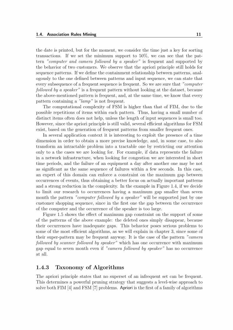
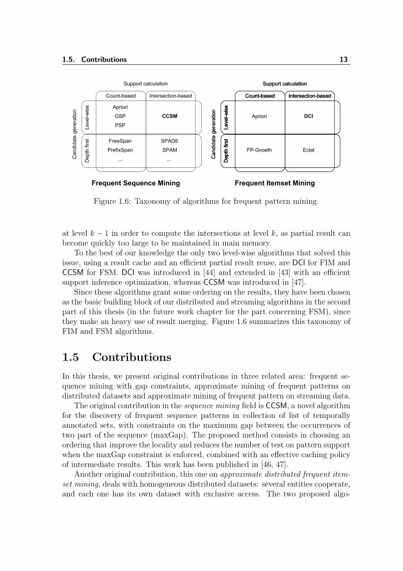
based on this method. First, every frequent item is found, and then the focus is onpairs composed of frequent items, and so on. Exploring the search space level-wisegrants that every time a new candidate is considered, the support of all its subpatterns is known. An alternative approach is the depth first discovery of frequentpatterns: by enforcing the apriori constraint just on some of the sub patterns, thesearch space is explored deeply. This is usually done in an attempt to preservelocality, examining consecutively similar patterns [25, 24, 52].
In both cases, the support of patterns is computed by updating a counter eachtime an occurrence is found. Moreover, when all the data fit in main memory, a moreefficient approach based on intersection can be devised. Each item x is associatedwith all the IDs of all transactions where x appears, and the support is equal to thesize of the intersection of the two sets. This set of IDs can be obtained using eitherbitmap [44] or tidlists [68]. In FSM, the technique is similar, but needs a longerdescription; an exhaustive explanation can be found in chapter 3.
The use of intersection in depth-first algorithms is highly efficient, thanks to theavailability of partial intersection results related to shorter patterns. For example,if we examine every pattern with a given prefix before moving to a different one,then the list of occurrences associated with that prefix can be reused, with littlewaste of memory, in the computations related to its descendant. However, theresults obtained are unsorted and this can be a problem in case the results areto be merged with other ones, as in case of mining on distributed and streamingdata, since we are forced to wait the end of the computation before being able tomerge the results. On the other hand, level-wise algorithms pose a strong obstacleto the efficient reuse of partial intersection results due to the limited locality in thesearch space traversal. When the search space is not partitioned as in the depth-first algorithm, it is impossible to exploit the partial intersection results computed
1.5. Contributions 13
Figure 1.6: Taxonomy of algorithms for frequent pattern mining.
at level k − 1 in order to compute the intersections at level k, as partial result canbecome quickly too large to be maintained in main memory.
To the best of our knowledge the only two level-wise algorithms that solved thisissue, using a result cache and an efficient partial result reuse, are DCI for FIM andCCSM for FSM. DCI was introduced in [44] and extended in [43] with an efficientsupport inference optimization, whereas CCSM was introduced in [47].
Since these algorithms grant some ordering on the results, they have been chosenas the basic building block of our distributed and streaming algorithms in the secondpart of this thesis (in the future work chapter for the part concerning FSM), sincethey make an heavy use of result merging. Figure 1.6 summarizes this taxonomy ofFIM and FSM algorithms.
1.5 Contributions
In this thesis, we present original contributions in three related area: frequent se-quence mining with gap constraints, approximate mining of frequent patterns ondistributed datasets and approximate mining of frequent pattern on streaming data.
The original contribution in the sequence mining field is CCSM, a novel algorithmfor the discovery of frequent sequence patterns in collection of list of temporallyannotated sets, with constraints on the maximum gap between the occurrences oftwo part of the sequence (maxGap). The proposed method consists in choosing anordering that improve the locality and reduces the number of test on pattern supportwhen the maxGap constraint is enforced, combined with an effective caching policyof intermediate results. This work has been published in [46, 47].
Another original contribution, this one on approximate distributed frequent item-set mining, deals with homogeneous distributed datasets: several entities cooperate,and each one has its own dataset with exclusive access. The two proposed algo-
14 1. Introduction
rithms [59, 61], allow for obtaining a good approximate solution, and need just onesynchronization in one case and none in the other. In APRed, the algorithm proposedin [59], each node begins the computation with a reduced support threshold. Aftera first phase, needed to understand the peculiarities of the dataset, the minimumsupport is increased again to an intermediate value chosen according to the behaviorof pattern computed during the first phase. Thereafter each node can continue inde-pendently and send, at the end of the computation, the result to the master, whichreconstructs an approximation of the set of all global frequent patterns. The goalof the support reduction is to force infrequent patterns to be revealed in partitionswhere they have nearly frequent support. The results obtained by this method areclose to the exact ones for several real-world datasets originated by shopping chartand web navigation. To the best of our knowledge, this is the first algorithm forapproximate distributed FIM based on an adaptive support reduction scheme.
Similar accuracy in the results, but with higher performance thanks to the asyn-chronous behavior and no support reduction, are achieved by the APInterp algorithmthat we have introduced in [61]. It is based on the interpolation of unknown patternsupports, based on the knowledge acquired from the other partitions.
The absence of synchronizations, and of any two-way communication between themaster and the worker nodes, makes APInterp suitable for streaming data, consideringeach new incoming block of data as a partition, and the rest of data as another one.In this way the merge and interpolate task can be applied repeatedly. This is thebasic idea of APStream, the algorithm we presented in [60]. In our tests on real worlddatasets, the results are similar to the exact ones, and the algorithm processes thestream in linear time.
The described interpolation framework can be easily extended to distributedstream and to the FSM problem, using the CCSM algorithm locally. A more chal-lenging extension, due to the subsumption-related result merging issues, concerns theapproximate distributed computation of Frequent Closed Itemsets (FCI), describedin our preliminary work [32]. Furthermore, the heuristic used in interpolation canbe easily substituted with another one, better fitted to the particular targeted appli-cation. However even the very simple and generic one used in our tests gives goodresults.
To the best of our knowledge, the AP method is the first distributed approachthat requires just one way communications (i.e., with global pruning optimizationdisabled, the worker nodes use only local information), tries to interpolate the miss-ing supports by exploiting the available knowledge and is suitable to both distributedand stream settings.
1.6 Thesis overview
This thesis is divided into self-contained chapters. Each chapter begins with as ashort overview containing an informal introduction to the subject and a description
1.6. Thesis overview 15
of the scope of the chapter. The first section in most chapters is usually a moreformal introduction to the problem, with definitions and references to related works.When other algorithms are used, either to describe the proposal contained in thecore of the chapter or its improvements in relation to the state of the art, thesealgorithms are described immediately after the introduction. The core part of thechapter contains an in depth description of the proposed method, followed by adiscussion on its pro and cons, and the descriptions of the experimental setup andresults. For the sake of readability, since parts of the citations are common to morechapters, the references are listed at the end of the thesis. For the same reason themeasures used for evaluating the approximation of the solutions are described inand appendix.
The first part of the thesis is made of two chapters that deal with algorithms thatwe will use in the following chapters about distributed and streaming data mining, aspreviously explained in the section about FIM and FSM algorithm taxonomy. Thefirst chapter introduces the frequent itemset mining problem and describes DCI [44],a state of the art algorithm for frequent itemset mining that we will use extensivelyin the rest of the thesis. The second chapter describes CCSM, a new algorithm forgap constrained sequence mining that we presented in [47].
In the second part of the thesis, the third chapter deals with approximate fre-quent itemset mining in homogeneous distributed datasets, and describes our twonovel approximate algorithms APRed and APInterp, based on support reduction andinterpolation. The fourth chapter extends the support interpolation method, in-troduced in the previous chapter, to streaming data [60]. Finally, the last chapterdescribes some future works and draws some conclusion. In particular, we describehow to extend the proposed interpolation framework in order to deal with frequentsequences, using CCSM in local computation. Moreover, we discern how to combinethe APInterp and APStream in an algorithm for the discovery of frequent itemset ondistributed data streams.

16 1. Introduction

IFirst Part

2Frequent Itemset Mining
Each data mining task has its peculiarities and issues when dealing with evolving anddistributed data, as we have briefly outlined in the introduction. A more detailedanalysis requires focusing on a particular task. In this thesis, we have decided toanalyze in detail this problem by discussing Association Rules Mining (ARM) andSequential Association Rules Mining (SARM), two of the most popular DM task.
The crucial steps in ARM, and by far the most computationally challenging, isthe extraction of frequent subsets from an input database of sets of distinct items,also known as Frequent Itemset Mining (FIM). In case the datasets is referred to theactivities of a shop, and data are sale transactions composed of several items, thegoal of FIM is to find the sets of items that are bought together, at least, in a userspecified number of transactions. The challenges in FIM derive from the large size ofits search space, which, in the worst case, corresponds to the power set of the set ofitems, and thus is exponential in the number of distinct items. Restricting as muchas possible this space and efficiently performing computations on the remaining partare key issues for FIM algorithms.
This chapter formally introduces the itemset mining problem and describes DCI(Direct Count and Intersect), a hybrid level-wise algorithm, which dynamicallyadapts its search strategy to the characteristics of the dataset and to the evolu-tion of the computation. This algorithm was introduced in [44], and extended in[43] with an efficient, key pattern based, support inference method.
With respect to the Frequent Pattern Mining algorithms taxonomy, presentedin the introduction, DCI is a level-wise algorithm, able to ensure an ordering ofthe results, and use an efficient hybrid counting strategy, switching to an in-coreintersection based support computation as soon as there is enough memory availablefor distributed and stream settings.
DCI has been chosen as the building block for our approximate algorithms dueto its efficiency, and the results ordering, which is particularly important whenmerging different result sets. Moreover, DCI exactly knows the exact amount ofmemory needed for the whole intersection phase before starting it, and this hasbeen exploited in APStream, our stream algorithm, for dynamically choosing the sizeof the block of transactions to process at once.

20 2. Frequent Itemset Mining
2.1 The problem
A dataset D is a collection of subsets of a set of items I = it1, . . . , itm. Each elementof D is called a transaction. A pattern x is frequent in dataset D, with respect toa minimum support minsup, if its support is greater than σmin = minsup · |D|,i.e., the pattern occurs in at least σmin transactions, where |D| is the number oftransactions in D. A k-pattern is a pattern composed of k items, Fk is the set ofall frequent k-patterns, and F =
⋃iFi is the set of all frequent patterns. F1 is also
called the set of frequent items. The computational complexity of the FIM problemderives from the exponential size of its search space P(M), i.e., the power set of M ,where M is the set of items contained in the various transactions of D.
2.1.1 Related works
A way to prune the search space P(M), first introduced in the Apriori [6] algorithm,is to restrict the search to itemsets whose subsets are all frequent. Apriori is a level-wise algorithm, since it examines the k-patterns only when all the frequent patternsof length k − 1 have been discovered. At each iteration k, a set of potentially fre-quent patterns, having all of their subset frequent, are generated starting from theprevious level results. Then the dataset is read sequentially, and the counters asso-ciated with each candidate are updated according to the occurrences founds. Afterthe database scan, only the candidates having a support greater than the thresholdare inserted in the result set and used for generating the next iteration candidates.Several other algorithms based on the apriori principle have been proposed. Someuse the same level wise approach, but introduce efficient optimizations, like a hy-brid count/intersection support computation [44] or the reduction of the number ofcandidates using a hash based technique [49]. Others use a depth-first approach,either class based [68] or projection based [2, 25]. Others again, use completelydifferent approaches, based on multiple independent computations on smaller partof the dataset, like [55, 50].
Related research topics are the discovery of maximal and closed frequent item-sets. The first ones are those frequent itemsets that are not included in any otherlarger frequent itemset. As an example, consider the FIM result set F = {{A} :4, {B} : 4, {C} : 3, {A, B} : 4, {A, C} : 3, {B, C} : 3, {A, B, C} : 3}, where thenotation set : count indicates frequent itemsets along with their supports. In thiscase there is only one maximal frequent pattern Fmax = {{A, B, C} : 3}, since theother itemsets are included in it. Clearly the algorithms that are able to mine di-rectly the set of maximal pattern, like [9, 3, 11], are faster and produce a morecompact output than FIM algorithms. Unfortunately, the information contained inthe result set are not the same: in the above example, there is no way to deducethe support of pattern A from Fmax. Frequent closed itemsets are those frequentitemsets that are set-included in any larger frequent itemset having the same sup-port. The group of patterns subsumed by the same itemset appears exactly in the
2.2. DCI 21
same set of transactions, and forms a class of equivalence, whose representative el-ement is the largest. Considering again the previous example, the patterns {A}and {B} are subsumed by the pattern {A, B} whereas the patterns {C}, {A, C}and {B, C} are subsumed by {A, B, C}. Thus, the set of frequent closed itemsetsis Fclosed = {{A, B} : 4, {A, B, C} : 3}. Note that in this case the support of anyfrequent itemset can be deduced as the support of its smaller superset contained inthe result, thus the {A, C} pattern support equal to 3, i.e., it has the same supportthan the pattern {A, B, C}.
2.2 DCI
The approximate algorithms that we will propose in the second part of the thesisfor distributed and stream data are build on traditional FPM algorithms, used forlocal computations. The partial ordering of results, the foreseeable resource usage,and the ability to recompute quickly a pattern support using the in-core verticalbitmap, made DCI our algorithm of choice.
DCI is a multi-strategy algorithm that runs in two phases, both level-wise. Duringits initial count-based phase, DCI exploits an out-of-core horizontal database, withvariable-length records. At the beginning of each iteration k, a set Ck of k-candidatesis generated, based on the frequent patterns contained in Fk−1, then their number ofoccurrences is verified during a database scan. At the end of the scan, the itemsetsin Ck having a support greater than the threshold σmin are inserted into Fk. Asexecution progress, the dataset size is reduced by removing transactions and itemsno longer needed for computation using a technique inspired by DHP [49]. As soon asthe pruned dataset becomes small enough to fit in memory, DCI adaptively changesits behavior. It builds a vertical layout database in-core, and starts adopting anintersection-based approach to determine frequent sets.
During this second phase DCI uses intersections to check the support of k-candidates, generated on the fly by composing all the pairs of (k − 1)-itemsetsthat are included in Fk−1 and share a common (k − 2)-prefix. When a candidateis found to be frequent, it is inserted into Fk. In order to ensure high spatial andtemporal locality, each Fi is maintained lexicographically ordered. This grants that(k−1)-patterns sharing a common prefix are stored contiguously in Fk−1 and, at thesame time, the candidates are considered in lexicographical order, thus granting theordering of the result. Furthermore, this allows accessing previous iteration resultsfrom disk in a nearly sequential way and storing immediately each pattern as soonas it is discovered to be frequent.
DCI uses several optimization techniques, such as support counting inferencebased on key patterns [43] and heuristics to dynamically adapt to both dense andsparse datasets. Here, however we will put our attention only on candidate gener-ation and the counting/intersection phases. Also in the pseudo-code, contained inalgorithm 1, the code part related to optimizations has been removed.
22 2. Frequent Itemset Mining
2.2.1 Candidate generation
Candidates are generated in both phases, even if at different times. In the count-based phase, all the candidates are generated at the beginning of each iteration andthen their supports are verified, whereas in the intersection-based one, the candi-dates are generated and their supports are checked on the fly. Another importantdifference concerns the memory usage: during the first phase the candidates andthe results are maintained in memory and the dataset is on disk, whereas duringthe second phase the candidates are generated on the fly, the result are immediatelyoffloaded to disk, and the dataset is kept in main memory.
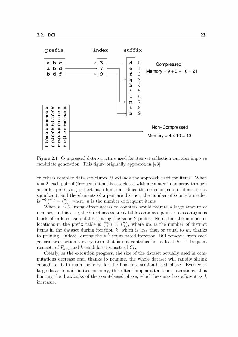
The generation of candidates of length k is based on the composition of pat-terns of k − 1 items sharing the same k − 2 long prefix. For example, if F2 ={A, B}, {A, C}, {A, D}, {B, C} is the set of frequent 2-patterns, then the set ofcandidates for the 3rd iteration will be C3 = {A, B, C}, {A, B, D}. DCI organizesitemsets of length k in a compressed data structure, optimized for spatial localityand fast access to groups of candidates sharing the same prefix, taking advantageof lexicographical ordering. A first array contains the k− 1 prefix and a second onecontains an index to the contiguous block of item suffixes contained in the thirdarray. Figure 2.1 shows the usage of these arrays. The patterns {A, B, D, M} and{A, B, D, I} are represented by the second prefix followed by the suffixes in positionsfrom 7 to 8, i.e., from the index position to the position before the one associated tothe next prefix. Generating the candidates using this data structure is straightfor-ward, and simply consists of the generation of all the pairs for each block of suffixes.E.g. for the block corresponding to the prefix {A, B, C}, {A, B, D, G} is inserted incandidate prefixes, with suffixes H,I and L, followed by {A, B, D, H} with suffixesI and L, followed {A, B, D, I} with suffix L.
Not every generated candidate obeys the apriori principle, so we can observe thatthe candidate pattern {A, B, D}, in the first example, cannot be frequent, since itssubpattern {B, D} is not frequent. When the candidates are stored in memory,during the counting-based phase, the apriori principle is enforced before insertingcandidates into candidate set. On the other hand, checking the presence of everysubset has a cost, which increases as the patterns get longer. If we also consider thatthe relevant subpatterns are not in any particular order, this disrupts both spatialand temporal locality in the access to the previous iteration results (Fk−1). For thisreason, and the low cost and high locality of intersection-based support checking, theauthors has decided to limit the candidate pruning step to the count-based phase.
2.2.2 Counting phase
In the first iteration, similarly to all FSC algorithms, DCI exploits a vector of coun-ters. In subsequent iterations, it uses a Direct Count technique, introduced by thesame authors in [42]. The goal of this technique is to make the access to the coun-ters associated with candidates as fast as possible. So, instead of using a hash tree,
2.2. DCI 23
prefix
a b da b c
b d f
suffixindex
379
defghilmin
0123456789
a b c da b c ea b c fa b c ga b d ha b d ia b d la b d mb d f ib d f n
Memory = 4 x 10 = 40
Memory = 9 + 3 + 10 = 21
Compressed
Non−Compressed
Figure 2.1: Compressed data structure used for itemset collection can also improvecandidate generation. This figure originally appeared in [43].
or others complex data structures, it extends the approach used for items. Whenk = 2, each pair of (frequent) items is associated with a counter in an array throughan order preserving perfect hash function. Since the order in pairs of items is notsignificant, and the elements of a pair are distinct, the number of counters neededis m(m−1)
2=(
m2
), where m is the number of frequent items.
When k > 2, using direct access to counters would require a large amount ofmemory. In this case, the direct access prefix table contains a pointer to a contiguousblock of ordered candidates sharing the same 2-prefix. Note that the number oflocations in the prefix table is
(mk
2
)6(
m2
), where mk is the number of distinct
items in the dataset during iteration k, which is less than or equal to m, thanksto pruning. Indeed, during the kth count-based iteration, DCI removes from eachgeneric transaction t every item that is not contained in at least k − 1 frequentitemsets of Fk−1 and k candidate itemsets of Ck.
Clearly, as the execution progress, the size of the dataset actually used in com-putations decrease and, thanks to pruning, the whole dataset will rapidly shrinkenough to fit in main memory, for the final intersection-based phase. Even withlarge datasets and limited memory, this often happen after 3 or 4 iterations, thuslimiting the drawbacks of the count-based phase, which becomes less efficient as kincreases.

24 2. Frequent Itemset Mining
Algorithm 1: DCI
input : D, minsup
// find the frequent itemsets ;1
F1 ← first scan(D, minsup);2
//second and following scans on a temporary db D′;3
F2 ← second scan(D′, minsup);4
k← 2;5
while D′.vertical size() > memory available() do6
k← k + 1;7
Fk ← DCI count(D′, minsup, k);8
end9
k← k + 1;10
// count-based iteration and create vertical database VD ;11
Fk ← DCI count(D′, VD, minsup, k);12
while Fk 6= ∅ do13
k← k + 1;14
Fk ← DCI intersect(VD, minsup, k) ;15
end16
2.2.3 Intersection phase
The intersection-based phase uses a vertical database, in which each item α is pairedwith a set of transactions tids(α) containing α, different from the horizontal oneused before, in which a set of items is associated with each transaction. Since atransaction t supports pattern x iff x ⊆ t, the set of transactions supporting x canbe obtained by intersecting the sets of transactions (tidlist) associated with eachitems in x. Thus the support σ(x) of a pattern x will be
σ(x) =
∣∣∣∣∣⋂α∈x
tids(α)
∣∣∣∣∣In DCI the sets of transactions are represented as bit-vectors, where the ith bit is equalto 1 when the ith transactions contains the item and is equal to 0 otherwise. Thisrepresentation allows for efficient intersections-based on the bitwise and operator.The memory necessary to contain this bitmap-based vertical representation is mk ·nk
bits, where mk and nk are respectively the numbers of items and transactions in thepruned database used at iteration k. As soon as this amount is less than the availablememory, the vertical dataset representation can be built on the fly in main memoryin order to begin the intersection based phase of DCI.
During this phase, the candidates are generated on the fly in lexicographicalorder, and their supports are checked using tidlist intersections. The above-describedmethod for support computation is indicated as k-way intersection. The k bit-vectors
2.3. Conclusions 25
associated with items contained in a k-pattern are and-intersected and the supportis obtained as the number of 1’s present in the resulting bit-vector. If this value isgreater than the support threshold σmin, then the candidate is inserted into Fk.
Since the candidates are generated on the fly, the set of candidates needs nolonger to be maintained. Moreover, both Fk−1 and Fk can be kept on disk. Indeed,Fk−1 is lexicographically ordered and can be loaded in block having the same (k−2)-prefix, and, thanks to the order of candidate generation, appending frequent patternsat the end of Fk preserves the lexicographic order.
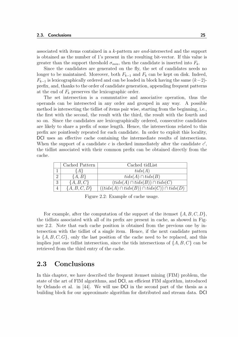
The set intersection is a commutative and associative operation, thus theoperands can be intersected in any order and grouped in any way. A possiblemethod is intersecting the tidlist of items pair wise, starting from the beginning, i.e.,the first with the second, the result with the third, the result with the fourth andso on. Since the candidates are lexicographically ordered, consecutive candidatesare likely to share a prefix of some length. Hence, the intersections related to thisprefix are pointlessly repeated for each candidate. In order to exploit this locality,DCI uses an effective cache containing the intermediate results of intersections.When the support of a candidate c is checked immediately after the candidate c′,the tidlist associated with their common prefix can be obtained directly from thecache.
Cached Pattern Cached tidList1 {A} tids(A)2 {A, B} tids(A) ∩ tids(B)3 {A, B, C} (tids(A) ∩ tids(B)) ∩ tids(C)4 {A, B, C,D} ((tids(A) ∩ tids(B)) ∩ tids(C)) ∩ tids(D)
Figure 2.2: Example of cache usage.
For example, after the computation of the support of the itemset {A, B, C,D},the tidlists associated with all of its prefix are present in cache, as showed in Fig-ure 2.2. Note that each cache position is obtained from the previous one by in-tersection with the tidlist of a single item. Hence, if the next candidate patternis {A, B, C,G}, only the last position of the cache need to be replaced, and thisimplies just one tidlist intersection, since the tids intersections of {A, B, C} can beretrieved from the third entry of the cache.
2.3 Conclusions
In this chapter, we have described the frequent itemset mining (FIM) problem, thestate of the art of FIM algorithms, and DCI, an efficient FIM algorithm, introducedby Orlando et al. in [44]. We will use DCI in the second part of the thesis as abuilding block for our approximate algorithm for distributed and stream data. DCI
26 2. Frequent Itemset Mining
has been chosen among the other FIM algorithms thanks to its efficiency and theresult ordering, which is particularly important when merging different result sets.Moreover, we can exactly predict the exact amount of memory needed by DCI for thewhole intersection phase before starting it, and this has been exploited in APStream,our stream algorithm, for dynamically choosing the size of the block of transactionsto process at the same time.
3Frequent Sequence Mining
The previous chapter has introduced the Frequent Itemset Mining (FIM) Problem,the most computationally challenging part of Association Rules Mining. This chap-ter deals with Sequential Association Rules Mining (SARM) and in particular withits Frequent Sequence Mining (FSM) phase. In this thesis work we have decided tofocus on this two popular data mining tasks, with particular regard to the issuesrelated to distributed and stream settings, and the usage of approximate algorithmsin order to overcome these problems. The algorithm proposed in this chapter, canbe used as a building block for the Frequent Sequence version of our approximatedistributed and stream algorithms described in the second part of this thesis, thanksto its efficiency, and results ordering, which is particularly important when mergingdifferent result sets.
The frequent sequence mining (FSM) problem consists in finding frequent sequen-tial patterns in a database of time-stamped events. Going on with the supermarketexample, market baskets are linked to a time-line and no longer anonymous. An im-portant extension to the base FSM problem is the introduction of time constraints.For example, several application domains require limiting the maximum temporalgap between events occurring in the input sequences. However pushing down thisconstraint is critical for most sequence mining algorithms.
This chapter formally introduces the sequence mining problem and proposesCCSM (Cache-based Constrained Sequence Miner), a new level-wise algorithm thatovercomes the troubles usually related to this kind of constraint. CCSM adopts aninnovative approach based on k-way intersections of idlists to compute the supportof candidate sequences. Our k-way intersection method is enhanced by the useof an effective cache that stores intermediate idlists for future reuse inspired byDCI [44] (see previous chapter). The reuse of intermediate results entails a surprisingreduction in the actual number of join operations performed on idlists.
CCSM has been experimentally compared with cSPADE [69], a state of the artalgorithm, on several synthetically generated datasets, obtaining better or similarresults in most cases.
Since some concept introduced in GSP [62] and SPADE [70] algorithm are usedto explain the CCSM algorithm, a quick description of these two follows the problemdescription. Other related works are referred at the end of the chapter.
28 3. Frequent Sequence Mining
3.1 Introduction
The problem of mining frequent sequential patterns was introduced by Agarwal andSrikant in [7]. In a subsequent work, the same authors discussed the introduction ofconstraints on the mined sequences, and proposed GSP [62], a new algorithm dealingwith them. In the last years, many innovative algorithms were presented for solvingthe same problem, also under different user-provided constraints [69, 70, 53, 20, 52,8].
We can think of the problem of mining Frequent Sequence Mining (FSM) asa generalization of Frequent Itemset Mining (FIM) to temporal databases. FIMalgorithms aims to find patterns (itemsets) occurring with a given minimum supportwithin a transactional database D, whose transactions correspond to collections ofitems. A pattern is frequent if its support is greater than (or equal to) a giventhreshold s%, i.e. if it is set-included in at least s%·|D| input transactions, where |D|is the total number of transactions in D. An input database D for the FSM problemis instead composed of a collection of sequences. Each sequence corresponds to atemporally ordered list of events, where each event is a collection of items (itemset)occurring simultaneously. The temporal ordering among the events is induced fromthe absolute timestamps associated with the events.
A sequential pattern is frequent if its support is greater than (or equal to) agiven threshold s%, i.e. if it is ”contained” in (or it is a subsequence of) at leasts% · |D| input sequences, where |D| is the number of sequences included in D.
To make more intuitive both problem formulations, we may consider them withinthe application context of the market basket analysis (MBA). In this context, eachtransaction (itemset) occurring in a database D of the FIM problem corresponds tothe collection of items purchased by a customer during a single visit to the market.The FIM problem for MBA consists in finding frequent associations among the itemspurchased by customers. In the general case, we are thus not interested in the time-stamp of each purchased basket, or in the identity of its customer, so the inputdatabase does not need to store such information. Conversely, FSM problem forMBA consists in predicting customer behaviors on the basis of their past purchases.Thus, D has also to include information about timestamp and customer identityof each basket. The sequences of events included in D correspond to sequencesof ”baskets” (transactions) purchased by the same customer during distinct visitsto the market, and the items of a sequential pattern can span a set of subsequenttransactions belonging to the same customer. Thus, while the FIM problem isinterested in finding intra-transaction patterns, the FSM problem determines inter-transaction sequential patterns.
Due to the similarities between the FIM and FSM problems, several FIM al-gorithms have been adapted for mining frequent sequential patterns as well. LikeFIM algorithms, also FSM ones can adopt either a count-based or intersection-basedapproach for determining the support of frequent patterns. The GSP algorithm,which is derived from Apriori [7], adopts a count-based approach, together with a
3.1. Introduction 29
level-wise visit (Breadth-First) of the search space. At each iteration k, a set ofcandidate k-sequences (sequences of length k) is generated, and the dataset, storedin horizontal form, is scanned to count how many times each candidate is containedwithin each input sequences. The other approach, i.e. the intersection-based one,relies on a vertical-layout database, where for each item X appearing in the vari-ous input sequences we store an idlist L(X). The idlist contains information aboutthe identifiers of the input sequences (sid) that include X, and the timestamps(eid) associated with each occurrence of X. Idlists are thus composed of pairs (sid,eid), and are considerably more complex than the lists of transaction identifiers(tidlists) exploited by intersection-based FIM algorithms. Using an intersection-based method, the support of a candidate is determined by joining lists. In the FIMcase, tidlist joining is done by means of simple set-intersection operations. Con-versely, idlist joining in FSM intersection-based algorithms exploits a more complextemporal join operation. Zaki’s SPADE algorithm [70] is the best representative ofsuch intersection-based FSM algorithms.
Several real applications of FSM enforce specific constraints on the type of se-quences extracted [62, 53]. For example, we might be interested in finding frequentsequences of purchase events which contain a given subsequence (super pattern con-straint), or where the average price of items purchased is over a given threshold(aggregate constraint), or where the temporal intervals between each pair of con-secutive purchases is below a given threshold (maxGap constraint). Obviously, wecould solve this problem with a post-processing phase: first, we extract from thedatabase all the frequent sequences, and then we filter them on the basis of theposed constraints. Unfortunately, when the constraint is not on the sequence itselfbut on its occurrences (as in the case of the maxGap constraint), sequence filter-ing requires an additional scan of the database to verify whether a given frequentpattern has still a minimum support under the constraint. In general, FSM algo-rithms that directly deal with user-provided constraints during the mining processare much more efficient, since constraints may involve an effective prune of candi-dates, thus resulting in a strong reduction of the computational cost. Unfortunately,the inclusion of some support-related constraints may require large modifications inthe code of an unconstrained FSM algorithm. For example, the introduction of themaxGap constraint in the SPADE algorithm, gave rise to cSPADE, a very differentalgorithm [69].
All the FSM algorithms rely on the anti-monotonic property of sequence fre-quency: every subsequence of a frequent sequence is frequent as well. More preciselymost algorithms rely on a weaker property, restricted to a well-characterized partof subsets. This property is used to generate candidate k-sequence from frequent(k − 1)-sequences. When an intersection-based approach is adopted, we can deter-mine the support of any k-sequence by means of join operations performed [55] onthe idlist associated with its subsequences. As a limit case, we could compute thesupport of a sequence by joining the atomic idlists associated with the single itemsincluded in the sequence, i.e., through a k-way join operation [44]. More efficiently,
30 3. Frequent Sequence Mining
we could compute the support of a sequence by joining the idlists associated withtwo generating (k − 1)-subsequences, i.e., through a 2-way join operation. SPADE[70] just adopts this 2-way intersection method, and computes the support of a k-sequence by joining two of its (k − 1)-subsequences that share a common suffix.Unfortunately, the adoption of 2-way intersections requires maintaining the idlistsof all the (k − 1)-subsequences computed during the previous iteration. To limitmemory requirement, SPADE subdivides the search space into small, manageablechunks. This is accomplished by exploiting suffix-based equivalence classes: twok-sequences are in the same class only if they share a common (k − 1)-suffix. Sinceall the generating subsequences of a given sequence belong to the same equivalenceclass, equivalence classes are used to partition the search space in a way that alloweach class to be processed independently in memory. Unfortunately, the efficientmethod used by SPADE to generate candidates and join their idlists, cannot be ex-ploited when a maximum gap constraint is considered. Therefore, cSPADE is forcedto adopt a different and much more expensive way to generate sequences and joinidlists, also maintaining in memory F2, the set of frequent 2-sequences.
This chapter discuss CCSM (Cache-based Constrained Sequence Miner), a newlevel-wise intersection-based FSM algorithm, dealing with the challenging maximumgap constraint. The main innovation of CCSM is the adoption of k-way intersectionsto compute the support of candidate sequences. Our k-way intersection method isenhanced by the use of an effective cache, which store intermediate idlists. The idlistreuse allowed by our cache entails a surprising reduction in the actual number of joinoperations performed, so that the number of joins performed by CCSM approachesthe number of joins performed when a pure 2-way intersection method is adopted,but require much less memory. In this context, it becomes interesting to comparethe performances of CCSM with the ones achieved by cSPADE when a maximumgap constraint is enforced.
The rest of the chapter is organized as follows. Section 3.2 formally defines theFSM problem, while Section 3.5.2 describes the CCSM algorithm. In Section 3.5.3,there are some experimental results and a discussion about them. Finally, Section 5.4presents some concluding remarks.
3.2 Sequential patterns mining
3.2.1 Problem statement
Definition 1. (Sequence of events) Let I = {i1, ..., im} be a set of m distinctitems. An event (itemset) is a non-empty subset of I. A sequence is a temporallyordered list of events. We denote an event as (j1, . . . , jm) and a sequence as (α1 →. . . → αk), where each ji is an item and each αi is an event (ji ∈ I and αi ⊆ I).The symbol → denotes a happens-after relationship. The items that appear togetherin an event happen simultaneously. The length |x| of a sequence x is the number
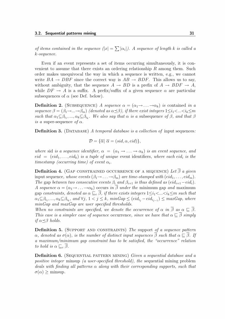
3.2. Sequential patterns mining 31
of items contained in the sequence (|x| =∑|αi|). A sequence of length k is called a
k-sequence.
Even if an event represents a set of items occurring simultaneously, it is con-venient to assume that there exists an ordering relationship R among them. Suchorder makes unequivocal the way in which a sequence is written, e.g., we cannotwrite BA → DBF since the correct way is AB → BDF . This allows us to say,without ambiguity, that the sequence A → BD is a prefix of A → BDF → A,while DF → A is a suffix. A prefix/suffix of a given sequence α are particularsubsequences of α (see Def. below).
Definition 2. (Subsequence) A sequence α = (α1→ . . .→αk) is contained in asequence β = (β1→...→βm) (denoted as α�β), if there exist integers 1≤i1<...<ik≤msuch that α1⊆βi1 , ..., αk⊆βik . We also say that α is a subsequence of β, and that βis a super-sequence of α.
Definition 3. (Database) A temporal database is a collection of input sequences:
D = {α| α = (sid, α, eid)},
where sid is a sequence identifier, α = (α1 → . . .→ αk) is an event sequence, andeid = (eid1, . . . , eidk) is a tuple of unique event identifiers, where each eidi is thetimestamp (occurring time) of event αi.
Definition 4. (Gap constrained occurrence of a sequence) Let β a giveninput sequence, whose events (β1→ . . .→βm) are time-stamped with (eid1, . . . , eidm).The gap between two consecutive events βi and βi+1 is thus defined as (eidi+1−eidi).A sequence α = (α1→ . . .→αk) occurs in β under the minimum gap and maximumgap constraints, denoted as α vc β, if there exists integers 1≤i1<...<ik≤m such thatα1⊆βi1 , ..., αk⊆βik , and ∀j, 1 < j ≤ k, minGap ≤ (eidij −eidij−1
) ≤ maxGap, whereminGap and maxGap are user specified thresholds.When no constraints are specified, we denote the occurrence of α in β as α v β.This case is a simpler case of sequence occurrence, since we have that α v β simplyif α�β holds.
Definition 5. (Support and constraints) The support of a sequence patternα, denoted as σ(α), is the number of distinct input sequences β such that α v β. Ifa maximum/minimum gap constraint has to be satisfied, the “occurrence” relationto hold is α vc β.
Definition 6. (Sequential pattern mining) Given a sequential database and apositive integer minsup (a user-specified threshold), the sequential mining problemdeals with finding all patterns α along with their corresponding supports, such thatσ(α) ≥ minsup.
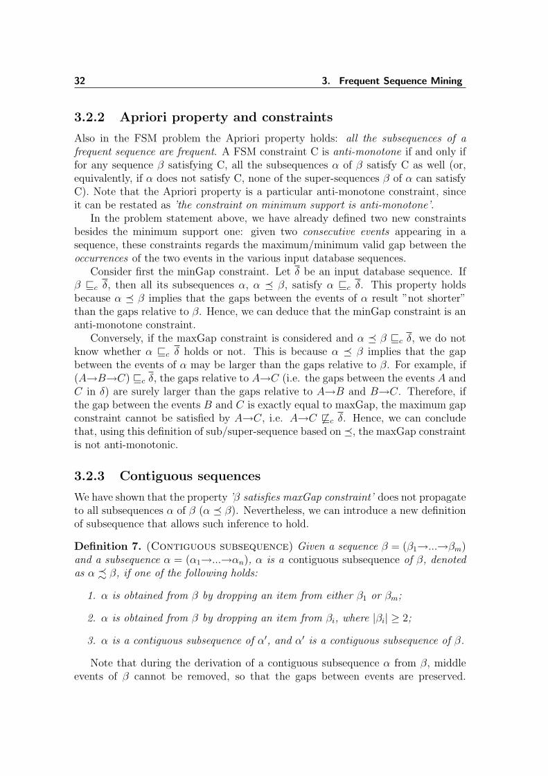
32 3. Frequent Sequence Mining
3.2.2 Apriori property and constraints
Also in the FSM problem the Apriori property holds: all the subsequences of afrequent sequence are frequent. A FSM constraint C is anti-monotone if and only iffor any sequence β satisfying C, all the subsequences α of β satisfy C as well (or,equivalently, if α does not satisfy C, none of the super-sequences β of α can satisfyC). Note that the Apriori property is a particular anti-monotone constraint, sinceit can be restated as ’the constraint on minimum support is anti-monotone’.
In the problem statement above, we have already defined two new constraintsbesides the minimum support one: given two consecutive events appearing in asequence, these constraints regards the maximum/minimum valid gap between theoccurrences of the two events in the various input database sequences.
Consider first the minGap constraint. Let δ be an input database sequence. Ifβ vc δ, then all its subsequences α, α � β, satisfy α vc δ. This property holdsbecause α � β implies that the gaps between the events of α result ”not shorter”than the gaps relative to β. Hence, we can deduce that the minGap constraint is ananti-monotone constraint.
Conversely, if the maxGap constraint is considered and α � β vc δ, we do notknow whether α vc δ holds or not. This is because α � β implies that the gapbetween the events of α may be larger than the gaps relative to β. For example, if(A→B→C) vc δ, the gaps relative to A→C (i.e. the gaps between the events A andC in δ) are surely larger than the gaps relative to A→B and B→C. Therefore, ifthe gap between the events B and C is exactly equal to maxGap, the maximum gapconstraint cannot be satisfied by A→C, i.e. A→C 6vc δ. Hence, we can concludethat, using this definition of sub/super-sequence based on �, the maxGap constraintis not anti-monotonic.
3.2.3 Contiguous sequences
We have shown that the property ’β satisfies maxGap constraint’ does not propagateto all subsequences α of β (α � β). Nevertheless, we can introduce a new definitionof subsequence that allows such inference to hold.
Definition 7. (Contiguous subsequence) Given a sequence β = (β1→...→βm)and a subsequence α = (α1→...→αn), α is a contiguous subsequence of β, denotedas α - β, if one of the following holds:
1. α is obtained from β by dropping an item from either β1 or βm;
2. α is obtained from β by dropping an item from βi, where |βi| ≥ 2;
3. α is a contiguous subsequence of α′, and α′ is a contiguous subsequence of β.
Note that during the derivation of a contiguous subsequence α from β, middleevents of β cannot be removed, so that the gaps between events are preserved.
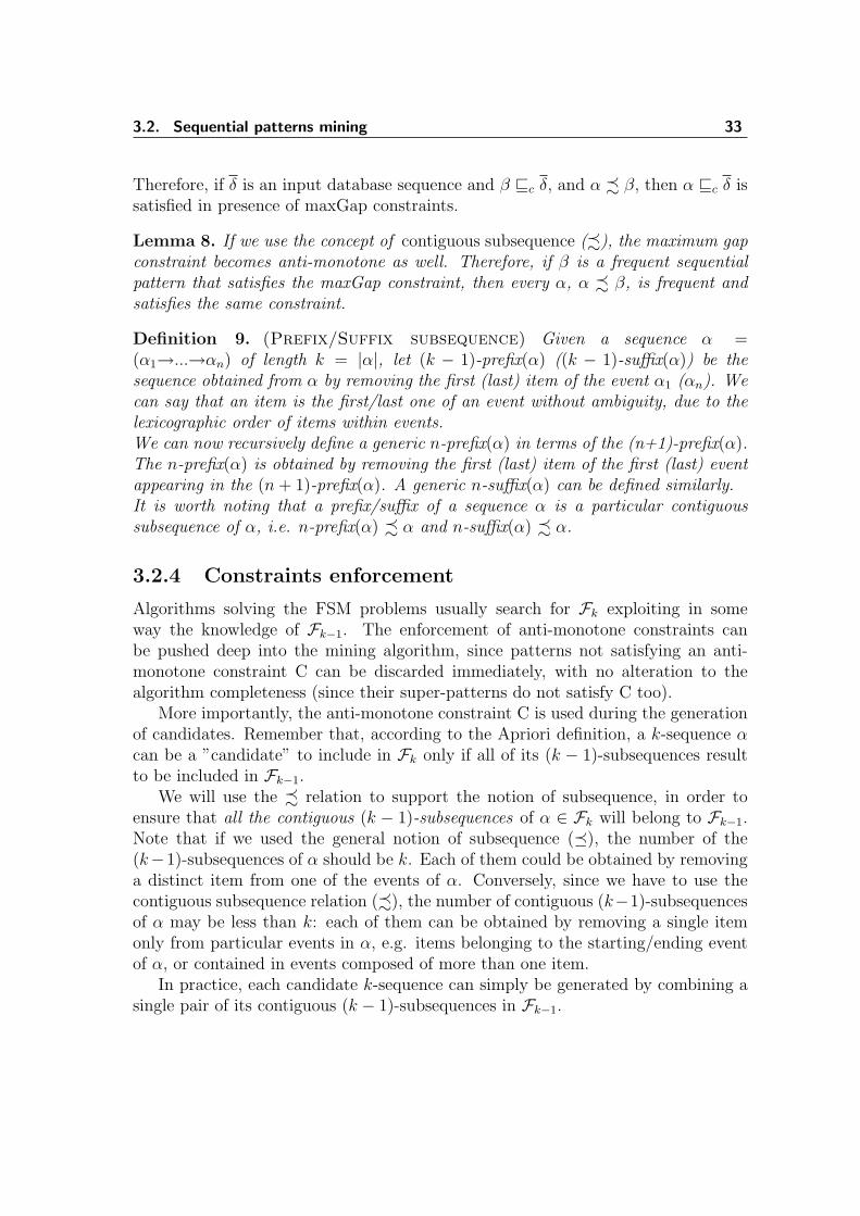
3.2. Sequential patterns mining 33
Therefore, if δ is an input database sequence and β vc δ, and α - β, then α vc δ issatisfied in presence of maxGap constraints.
Lemma 8. If we use the concept of contiguous subsequence (-), the maximum gapconstraint becomes anti-monotone as well. Therefore, if β is a frequent sequentialpattern that satisfies the maxGap constraint, then every α, α - β, is frequent andsatisfies the same constraint.
Definition 9. (Prefix/Suffix subsequence) Given a sequence α =(α1→...→αn) of length k = |α|, let (k − 1)-prefix(α) ((k − 1)-suffix(α)) be thesequence obtained from α by removing the first (last) item of the event α1 (αn). Wecan say that an item is the first/last one of an event without ambiguity, due to thelexicographic order of items within events.We can now recursively define a generic n-prefix(α) in terms of the (n+1)-prefix(α).The n-prefix(α) is obtained by removing the first (last) item of the first (last) eventappearing in the (n + 1)-prefix(α). A generic n-suffix(α) can be defined similarly.It is worth noting that a prefix/suffix of a sequence α is a particular contiguoussubsequence of α, i.e. n-prefix(α) - α and n-suffix(α) - α.
3.2.4 Constraints enforcement
Algorithms solving the FSM problems usually search for Fk exploiting in someway the knowledge of Fk−1. The enforcement of anti-monotone constraints canbe pushed deep into the mining algorithm, since patterns not satisfying an anti-monotone constraint C can be discarded immediately, with no alteration to thealgorithm completeness (since their super-patterns do not satisfy C too).
More importantly, the anti-monotone constraint C is used during the generationof candidates. Remember that, according to the Apriori definition, a k-sequence αcan be a ”candidate” to include in Fk only if all of its (k − 1)-subsequences resultto be included in Fk−1.
We will use the - relation to support the notion of subsequence, in order toensure that all the contiguous (k − 1)-subsequences of α ∈ Fk will belong to Fk−1.Note that if we used the general notion of subsequence (�), the number of the(k−1)-subsequences of α should be k. Each of them could be obtained by removinga distinct item from one of the events of α. Conversely, since we have to use thecontiguous subsequence relation (-), the number of contiguous (k−1)-subsequencesof α may be less than k: each of them can be obtained by removing a single itemonly from particular events in α, e.g. items belonging to the starting/ending eventof α, or contained in events composed of more than one item.
In practice, each candidate k-sequence can simply be generated by combining asingle pair of its contiguous (k − 1)-subsequences in Fk−1.
34 3. Frequent Sequence Mining
3.3 GSP
The first algorithm that proposed this candidate generation method, based on pairsof contiguous sequences, was presented in [62] by Srikant and Agrawal. Their algo-rithm, GSP, is a level-wise algorithm that scans repeatedly the dataset, and countsthe occurrences of the candidate frequent patterns contained in a set, which is gen-erated before the beginning of each iteration. Each k-candidates is generated bymerging a pair of frequent (k − 1)-patterns that share a (k − 2) long contiguoussub-sequence.
Figure 3.1: GSP candidate generation. The 3-patterns and 4-patterns are connectedwith their generators using a thick line. Candidates discarded after support checkare not shown.
3.3.1 Candidate generation
During the k-candidate generation phase, GSP merges every pair of frequent (k−1)-patterns α and β, such that (k − 2) − suffix(α) = (k − 2) − prefix(β). Theresult of the merge is pattern α concatenated with the last item contained in β,1 − suffix(β). This item is inserted as part of the last event, if this was thecase in β, or as a new event otherwise. For example, the patterns A → B andB → C generate the candidate A → B → C, whereas the patterns A → B andBC generate the candidate A → BC. In case some of the k − 1-subsequences ofthe obtained candidate are not frequent, the candidate is discarded. In the aboveexample, in case A→ C is not frequent, A→ BC can be safely discarded. However,the same is not true, for A → B → C, since A → C is not one of its contiguoussubsequences. Indeed, even in case A → C was not frequent due to the maxGapconstraint, A→ B → C could be frequent.
3.4. SPADE 35
The set of candidates Ck is represented using a hash tree. Each node in the treeis either a leaf node, containing sequences along with their counters, or an internalnode, containing pointers to other nodes. In order to find the counter for a pattern,the tree is traversed starting from the root. The next branch to visit is chosen usinga hash function on the pth item in the sequence, where p is the depth of the node.
Figure 3.1 represents a lattice of frequent patterns. Each ellipse indicates a pat-tern, a line indicates the relationship includes/included by, and a thick line indicatesthe ones exploited by GSP for the generation of candidates containing more thantwo items.
3.3.2 Counting
As soon as GSP completes the generation of the set of candidates Ck, it start read-ing the input sequences in the dataset one by one. When an input sequence d isprocessed, GSP search the hash tree recursively, processing all the branches that arecompatibles with the time-stamps contained in d. Each time a leaf is reached, GSPcheck if any of the sequence patterns in the leaf is supported by d, and, in case thetime constraints are satisfied, it increments the associated counter. The inclusioncheck of sequence pattern s in the input sequence d is performed using a verticalrepresentation of d, i.e., each item in d is associated with a list of time-stampscorresponding to its occurrences in d. This representation enables GSP to align effi-ciently the pattern s with the input sequence d, starting from the first element andstretching gaps as long as the constraints are satisfied.
3.4 SPADE
A completely different approach was proposed by Zaki in SPADE [70]. SPADE is anintersection-based algorithm, i.e. each item is associated to a list of pairs (sid, eid)and the support of a pattern is obtained using intersections. The pair (sid, eid)corresponds to an occurrence of the items in an input sequence sid (sequence id)with time-stamp eid (event id). Since these lists are kept in memory, the candidatescan be generated and checked on the fly, and there is no need to maintain in memorythe set of candidates, or to scan the dataset multiple times.
SPADE, as GSP, merges pairs of (k−1)-patterns to obtain k-candidates, howeverthe pairs are chosen in a different way.
3.4.1 Candidate generation
SPADE generates a candidate k-sequence from a pair of frequent (k−1)-subsequencesthat share a common (k − 2)-prefix1. The generate candidate is composed of α
1In some version of the algorithm the author uses suffixes instead of prefixes. This is notrelevant, however, unless we need to restrict the search space to patterns beginning/ending with
36 3. Frequent Sequence Mining
followed by the last element of β, either as one-item event, or as part of the lastevent as we will explain later. For example, α = A→B→C→D is obtained bycombining the two subsequences A→B→C and A→B→D, which share the 2-prefixA→B. Since also the resulting candidates share the same prefixes, a set of k-patternssharing a common (k− 1)-prefix is closed with respect to candidate generation, andcan be processed independently. The generation of 2-candidates is in some way anexception: every pair of frequent items can generate candidates since they share a0-prefix. For this reason, SPADE use intersections for candidates containing at least3 items, but uses a count based approach for frequent items and 2-patterns.
In order to generate k-candidates, SPADE considers each pair of frequent (k−1)-patterns sharing the same (k − 2)-prefix, included pairs containing twice the samepattern. Each pair can produce one, two, three or no candidates at all, depending ontheir last events. Let α and β be two frequent (k − 1)-patterns sharing a commonprefix P and ending respectively with items X and Y . The last event in α maycontain one or more items. The first case is indicated as α = P → X, the secondone as α = PX. Four cases may arise:
α = P → X, β = P → YP → XY , P → X → Y and P → Y → X are valid candidates. Incase X = Y , P → X → X is the only candidate generated by α and β.
α = P → X, β = PYPY → X is the only candidate generated by α and β.
α = PX, β = P → YPX → Y is the only candidate generated by α and β.
α = PX, β = PYIn case X < Y , the candidate is PXY . Otherwise the candidate isPY X, unless X = Y . In this case, no candidate is generated.
3.4.2 Candidate support check
Immediately after the generation of a candidate, SPADE check its support usingidlist intersections. An idlist is a sorted list of the occurrences, i.e., pairs (sid, eid),where sid identifies a specific input sequence, and eid one of its events. The or-dering is on sid, with eid as secondary key. In SPADE, an idlist can be referredeither to an item or to a pattern. In the first case, the list corresponds to theoccurrences of the pattern, in the second case to the last position of each occur-rence of the sequence. For example, if the only input sequence in the dataset is(sid = 1, {({A, B}, eid = 1), ({A, C}, eid = 2), ({C}, eid = 6)}), then idlist(A) ={(1, 1), (1, 2)}, idlist(AC) = {(1, 2)}, and idlist(A → C) = {(1, 2), (1, 3)}. Note
some items or sequence of items.
3.5. CCSM 37
that it is not relevant that there are two distinct occurrences of A → C ending in(1, 3).
Two kind of intersection are possible: ordinary intersection, or equality join, andtemporal intersection, or temporal join. The first one is used when the candidateis PXY = αY , or P → XY = αY , and exactly corresponds to the commonset intersection of idlist(α) and idlist(Y ): the results is the set of pairs (sid, eid)appearing in both idlists. The second one is slightly more complex and correspondsto the candidates α → Y (PX → Y and P → X → Y ). In this case the results isthe subset of idlist(Y ) containing only those entries (sid, eid2) such that an entry(sid, eid1), with eid1 < eid2, exists in idlist(α). Thanks to the ordering of idlist bothoperation can be implemented efficiently. Furthermore, the idlist of α is availablefrom the previous level. Note that, thanks to the closure of common prefix classeswith respect to candidate generation, the search space can be traversed depth-firstby recursively exploring each prefix class. Thus, the idlist of prefixes can be reusedwith limited memory requirement. SPADE can also be implemented in a strictlylevel-wise manner, however it would be far less efficient.
3.4.3 cSPADE: managing constraints
In case the maxGap constraint is enforced, the solution found by the SPADE al-gorithm is no longer complete. For example, α = A→B→C→D is obtained bycombining the two subsequences A→B→C and A→B→D, which share the 2-prefixA→B. Unfortunately, A→B→D is not a contiguous subsequence of α. This im-plies that, even if α is frequent and satisfy a given maxGap constraint, i.e. α ∈ F4,its subsequence A→B→D could not have been included in F3 as not satisfyingthe same maxGap constraint. In other words, SPADE might loose candidates andrelative frequent sequences. cSPADE [69] overcomes this limit by exactly usingthe contiguous subsequence concept. α = A→B→C→D is now obtained fromA→B→C and C→D, i.e. by combining the (k − 1)-prefix and the 2-suffix of α. Itis straightforward to see that both the (k−1)-prefix and 2-suffix of α are contiguoussubsequences of α. Unfortunately, the need for contiguous subsequences to guaranteeanti-monotonicity under the maxGap constraint partially destroys the prefix-classequivalence self-inclusion of SPADE, which ensures high locality and low memoryrequirement. While each prefix-class is mined, cSPADE also needs to maintain F2
in the main memory, since it uses 2-suffixes to extend frequent (k − 1)-sequences.
3.5 CCSM
The reason behind the choice to use F2 for candidate generation in cSPADE, is thatF2 is usually smaller than Fk−1 for k > 3, so the idlists of frequent 2-sequences shouldfit in memory. However, even when this is true, the idlists of (k−1)-patterns containsmore elements, thus the average cost of an intersection is greater. In addition, the
38 3. Frequent Sequence Mining
number of intersection is generally increased. In fact, the generation of a candidatedepends on finding a pair of patterns with a matching common part. Hence, whenthe match is required on just one item, as in the case of intersection with F2, theprobability of generating a false positive (discarded candidate) is higher. On theother hand, since the suffixes of processed candidates are in no particular order,using Fk−1 for the same purpose, can be excessively memory demanding.
CCSM, the algorithm we propose, avoid these issues using a suitable traversalorder of the search space and an improved bidirectional idlist intersection operation.
3.5.1 Overview
The candidate generation method adopted by CCSM was inspired by GSP [62], whichis also based on the contiguous subsequence concept. We generate a candidate k-sequence α from a pair of frequent (k − 1)-sequences, which share with α either a(k − 2)-prefix or a (k − 2)-suffix. It easy to see that both these frequent (k − 1)-sequences are contiguous subsequences of α.
As we have already highlighted above, the candidates generated by cSPADE aremore than those generated by CCSM/GSP are. We show this with an example.Suppose that A → B → C ∈ F3, and that the only frequent 3-sequence havingprefix B → C is B → C → D. CCSM directly combines these two 3-sequencesto obtain a single potentially frequent 4-sequence A → B → C → D. Conversely,cSPADE tries instead to extend A→ B → C with all the 2-sequences in F2 that startwith C. In this way, cSPADE might generate a lot of candidates, even if, due to ourhypotheses, the only candidate that has chances to be frequent is A→ B → C → D.
3.5.2 The CCSM algorithm
Like GSP, CCSM visits level-wise and bottom-up the lattice of the frequent sequentialpatterns, building at each iteration Fk, the set of all frequent k-sequences.
CCSM starts with a count-based phase that mines a horizontal database, andextracts F1 and F2. During this phase, the database is scanned, and each inputsequence is checked against a set of candidate sequences. If the input sequencecontains a candidate sequence, the counter associated with the candidate is incre-mented accordingly. At the end of this count-based phase, the pruned horizontaldatabase is transformed into a vertical one, so that our intersection-based phase canstart. Thereinafter, when a candidate k-sequence is generated from a pair of frequent(k − 1)-patterns, its support is computed on-the-fly using items idlist intersections.This happens by joining the atomic idlists (stored in the vertical database) that areassociated with the frequent items in F1, as well as several previously computedintermediate idlists that are found in a cache.
In order to describe how the intersection-based phase works, it is necessary todiscuss how candidates are generated, how idlists are represented and joined, andhow CCSM idlist cache is organized.
3.5. CCSM 39
Candidate generation.
At iteration k, we generate the candidate k-sequences starting from the frequent(k − 1)-sequences in Fk−1. For each f ∈ Fk−1, we generate candidate k-sequencesby merging f with every f ′ ∈ Fk−1 such that (k − 2)-suffix(f) = (k − 2)-prefix(f ′).For example, f : BD→B is extended with f ′ : D→B→B to generate the candi-date 4-sequence BD→B→B. Note that by construction, f and f ′ are contiguoussubsequences of the new candidate.
To make more efficient the search in Fk−1 for pairs of sequences f and f ′ thatshare a common suffix/prefix, we aggregate and link the various groups of sequencesin Fk−1.
Figure 3.2 illustrates the generation of the candidate 4-sequences starting fromF3. On the left-hand and on the right-hand side of the figure two copies of the3-sequences in F3 are shown. These sequences are lexicographically ordered eitherwith respect to their 2-suffixes or to their 2prefixes. Moreover, sequences sharingthe same suffix/prefix are grouped (this is represented by circling each aggrega-tion/partition with dotted boxes). For example, a partition appearing on the leftside is {BD → B, D → D → B}. If two partitions that appear on the oppositesides share a common contiguous 2-subsequence (2-suffix = 2-prefix), they are alsolinked together. For instance, two linked partition are {BD → B, D → D → B}(on the left), and {D → BD, D → B → B} (on the right). Due to the sharing ofsuffix/prefix within and between linked partitions, we can obviously save memoryto represent F3.
The linked partitions of frequent sequential patterns are the only ones we mustcombine to generate all the candidates. In the middle of Figure 3.2, we show thecandidates generated for this example. Candidates than do not result frequent aredashed boxed, while the frequent ones are indicated with solid line boxes. Note that,before passing to the next pair, we first generate all the candidates from the currentpair of linked partitions. The order in which candidates are generated enhancestemporal locality, because the same prefix/suffix is encountered several times inconsecutively generated candidates. Our caching system takes advantage of thislocality, storing and reusing intermediate idlist joins.
Idlist intersection.
To determine the support of a candidate k-sequence p, we have first to produce theassociated idlist L(p). Its support will correspond to the number of distinct sidvalues contained in L(p).
To produce L(p), we have to join the idlists associated with two or more sub-sequences of p. If both L(p′1) and L(p′2) are available, where p′1 are p′2 are the twocontiguous subsequences whose combination produces p, L(p) can be generated veryefficiently through a 2-way intersection: L(p) = L(p′1) ∩ L(p′2). Otherwise, we haveto intersect idlists associated with smaller subsequences of p. The limit case is a
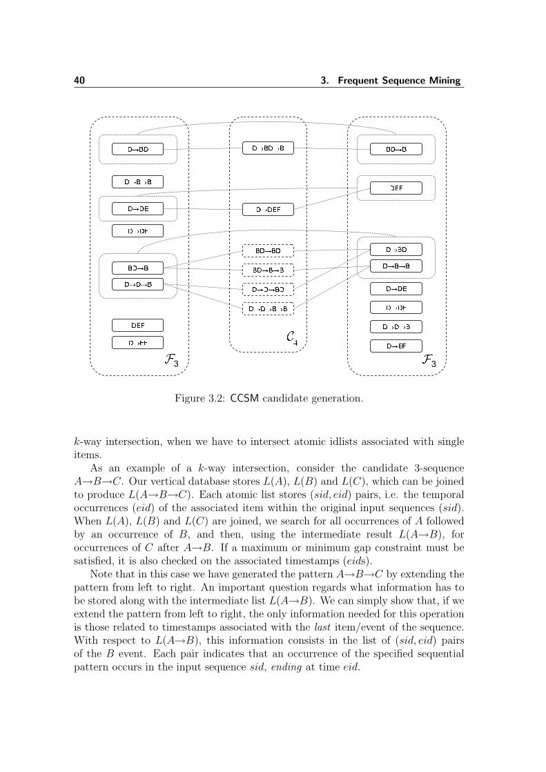
40 3. Frequent Sequence Mining
Figure 3.2: CCSM candidate generation.
k-way intersection, when we have to intersect atomic idlists associated with singleitems.
As an example of a k-way intersection, consider the candidate 3-sequenceA→B→C. Our vertical database stores L(A), L(B) and L(C), which can be joinedto produce L(A→B→C). Each atomic list stores (sid, eid) pairs, i.e. the temporaloccurrences (eid) of the associated item within the original input sequences (sid).When L(A), L(B) and L(C) are joined, we search for all occurrences of A followedby an occurrence of B, and then, using the intermediate result L(A→B), foroccurrences of C after A→B. If a maximum or minimum gap constraint must besatisfied, it is also checked on the associated timestamps (eids).
Note that in this case we have generated the pattern A→B→C by extending thepattern from left to right. An important question regards what information has tobe stored along with the intermediate list L(A→B). We can simply show that, if weextend the pattern from left to right, the only information needed for this operationis those related to timestamps associated with the last item/event of the sequence.With respect to L(A→B), this information consists in the list of (sid, eid) pairsof the B event. Each pair indicates that an occurrence of the specified sequentialpattern occurs in the input sequence sid, ending at time eid.
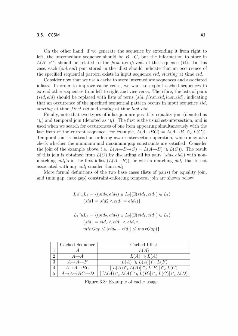
3.5. CCSM 41
On the other hand, if we generate the sequence by extending it from right toleft, the intermediate sequence should be B→C, but the information to store inL(B→C) should be related to the first item/event of the sequence (B). In thiscase, each (sid, eid) pair stored in the idlist should indicate that an occurrence ofthe specified sequential pattern exists in input sequence sid, starting at time eid.
Consider now that we use a cache to store intermediate sequences and associatedidlists. In order to improve cache reuse, we want to exploit cached sequences toextend other sequences from left to right and vice versa. Therefore, the lists of pairs(sid, eid) should be replaced with lists of terns (sid, first eid, last eid), indicatingthat an occurrence of the specified sequential pattern occurs in input sequence sid,starting at time first eid and ending at time last eid.
Finally, note that two types of idlist join are possible: equality join (denoted as∩e) and temporal join (denoted as ∩t). The first is the usual set-intersection, and isused when we search for occurrences of one item appearing simultaneously with thelast item of the current sequence: for example, L(A→BC) = L(A→B) ∩e L(C)).Temporal join is instead an ordering-aware intersection operation, which may alsocheck whether the minimum and maximum gap constraints are satisfied. Considerthe join of the example above, i.e. L(A→B→C) = L(A→B) ∩t L(C)). The resultof this join is obtained from L(C) by discarding all its pairs (sid2, eid2) with non-matching sid1’s in the first idlist (L(A→B)), or with a matching sid1 that is notassociated with any eid1 smaller than eid2.
More formal definitions of the two base cases (lists of pairs) for equality join,and (min gap, max gap) constraint-enforcing temporal join are shown below:
L1∩eL2 = {(sid2, eid2) ∈ L2|(∃(sid1, eid1) ∈ L1)
(sid1 = sid2 ∧ eid1 = eid2)}
L1∩tL2 = {(sid2, eid2) ∈ L2|(∃(sid1, eid1) ∈ L1)
(sid1 = sid2 ∧ eid1 < eid2∧minGap ≤ |eid2 − eid1| ≤ maxGap)}
Cached Sequence Cached Idlist1 A L(A)2 A→A L(A) ∩t L(A)3 A→A→B [L(A) ∩t L(A)] ∩t L(B)4 A→A→BC [[L(A) ∩t L(A)] ∩t L(B)] ∩e L(C)5 A→A→BC→D [[[L(A) ∩t L(A)] ∩t L(B)] ∩e L(C)] ∩t L(D)
Figure 3.3: Example of cache usage.
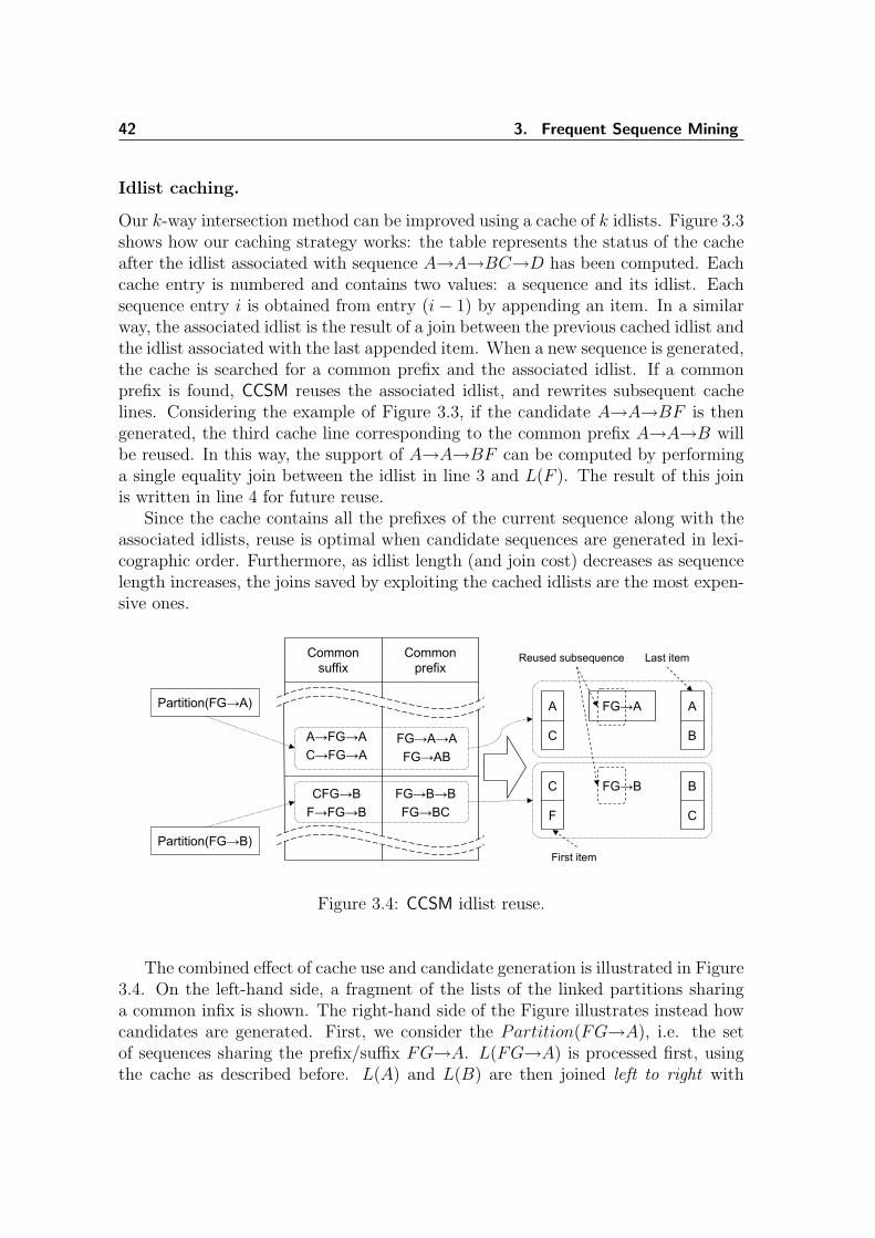
42 3. Frequent Sequence Mining
Idlist caching.
Our k-way intersection method can be improved using a cache of k idlists. Figure 3.3shows how our caching strategy works: the table represents the status of the cacheafter the idlist associated with sequence A→A→BC→D has been computed. Eachcache entry is numbered and contains two values: a sequence and its idlist. Eachsequence entry i is obtained from entry (i− 1) by appending an item. In a similarway, the associated idlist is the result of a join between the previous cached idlist andthe idlist associated with the last appended item. When a new sequence is generated,the cache is searched for a common prefix and the associated idlist. If a commonprefix is found, CCSM reuses the associated idlist, and rewrites subsequent cachelines. Considering the example of Figure 3.3, if the candidate A→A→BF is thengenerated, the third cache line corresponding to the common prefix A→A→B willbe reused. In this way, the support of A→A→BF can be computed by performinga single equality join between the idlist in line 3 and L(F ). The result of this joinis written in line 4 for future reuse.
Since the cache contains all the prefixes of the current sequence along with theassociated idlists, reuse is optimal when candidate sequences are generated in lexi-cographic order. Furthermore, as idlist length (and join cost) decreases as sequencelength increases, the joins saved by exploiting the cached idlists are the most expen-sive ones.
Figure 3.4: CCSM idlist reuse.
The combined effect of cache use and candidate generation is illustrated in Figure3.4. On the left-hand side, a fragment of the lists of the linked partitions sharinga common infix is shown. The right-hand side of the Figure illustrates instead howcandidates are generated. First, we consider the Partition(FG→A), i.e. the setof sequences sharing the prefix/suffix FG→A. L(FG→A) is processed first, usingthe cache as described before. L(A) and L(B) are then joined left to right with
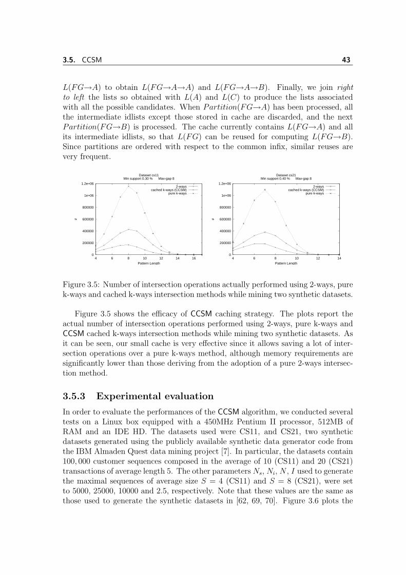
3.5. CCSM 43
L(FG→A) to obtain L(FG→A→A) and L(FG→A→B). Finally, we join rightto left the lists so obtained with L(A) and L(C) to produce the lists associatedwith all the possible candidates. When Partition(FG→A) has been processed, allthe intermediate idlists except those stored in cache are discarded, and the nextPartition(FG→B) is processed. The cache currently contains L(FG→A) and allits intermediate idlists, so that L(FG) can be reused for computing L(FG→B).Since partitions are ordered with respect to the common infix, similar reuses arevery frequent.
0
200000
400000
600000
800000
1e+06
1.2e+06
4 6 8 10 12 14 16
#
Pattern Length
Dataset cs11Min support 0.30 % Max-gap 8
2-wayscached k-ways (CCSM)
pure k-ways
0
200000
400000
600000
800000
1e+06
1.2e+06
4 6 8 10 12 14
#
Pattern Length
Dataset cs21Min support 0.40 % Max-gap 8
2-wayscached k-ways (CCSM)
pure k-ways
Figure 3.5: Number of intersection operations actually performed using 2-ways, purek-ways and cached k-ways intersection methods while mining two synthetic datasets.
Figure 3.5 shows the efficacy of CCSM caching strategy. The plots report theactual number of intersection operations performed using 2-ways, pure k-ways andCCSM cached k-ways intersection methods while mining two synthetic datasets. Asit can be seen, our small cache is very effective since it allows saving a lot of inter-section operations over a pure k-ways method, although memory requirements aresignificantly lower than those deriving from the adoption of a pure 2-ways intersec-tion method.
3.5.3 Experimental evaluation
In order to evaluate the performances of the CCSM algorithm, we conducted severaltests on a Linux box equipped with a 450MHz Pentium II processor, 512MB ofRAM and an IDE HD. The datasets used were CS11, and CS21, two syntheticdatasets generated using the publicly available synthetic data generator code fromthe IBM Almaden Quest data mining project [7]. In particular, the datasets contain100, 000 customer sequences composed in the average of 10 (CS11) and 20 (CS21)transactions of average length 5. The other parameters Ns, Ni, N , I used to generatethe maximal sequences of average size S = 4 (CS11) and S = 8 (CS21), were setto 5000, 25000, 10000 and 2.5, respectively. Note that these values are the same asthose used to generate the synthetic datasets in [62, 69, 70]. Figure 3.6 plots the
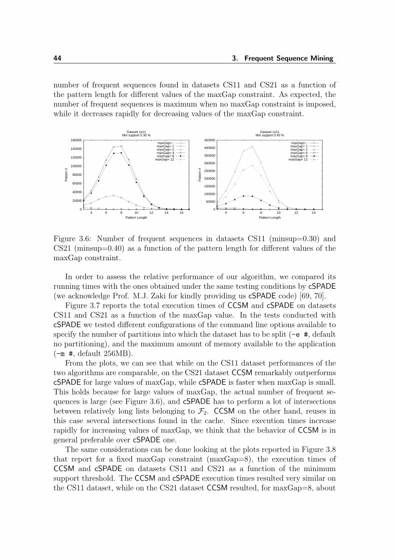
44 3. Frequent Sequence Mining
number of frequent sequences found in datasets CS11 and CS21 as a function ofthe pattern length for different values of the maxGap constraint. As expected, thenumber of frequent sequences is maximum when no maxGap constraint is imposed,while it decreases rapidly for decreasing values of the maxGap constraint.
0
20000
40000
60000
80000
100000
120000
140000
160000
4 6 8 10 12 14 16
Pat
tern
#
Pattern Length
Dataset cs11Min support 0.30 %
maxGap= -maxGap= 1maxGap= 2maxGap= 4maxGap= 8
maxGap= 12
0
50000
100000
150000
200000
250000
300000
350000
400000
450000
4 6 8 10 12 14
Pat
tern
#
Pattern Length
Dataset cs21Min support 0.40 %
maxGap= -maxGap= 1maxGap= 2maxGap= 4maxGap= 8
maxGap= 12
Figure 3.6: Number of frequent sequences in datasets CS11 (minsup=0.30) andCS21 (minsup=0.40) as a function of the pattern length for different values of themaxGap constraint.
In order to assess the relative performance of our algorithm, we compared itsrunning times with the ones obtained under the same testing conditions by cSPADE(we acknowledge Prof. M.J. Zaki for kindly providing us cSPADE code) [69, 70].
Figure 3.7 reports the total execution times of CCSM and cSPADE on datasetsCS11 and CS21 as a function of the maxGap value. In the tests conducted withcSPADE we tested different configurations of the command line options available tospecify the number of partitions into which the dataset has to be split (-e #, defaultno partitioning), and the maximum amount of memory available to the application(-m #, default 256MB).
From the plots, we can see that while on the CS11 dataset performances of thetwo algorithms are comparable, on the CS21 dataset CCSM remarkably outperformscSPADE for large values of maxGap, while cSPADE is faster when maxGap is small.This holds because for large values of maxGap, the actual number of frequent se-quences is large (see Figure 3.6), and cSPADE has to perform a lot of intersectionsbetween relatively long lists belonging to F2. CCSM on the other hand, reuses inthis case several intersections found in the cache. Since execution times increaserapidly for increasing values of maxGap, we think that the behavior of CCSM is ingeneral preferable over cSPADE one.
The same considerations can be done looking at the plots reported in Figure 3.8that report for a fixed maxGap constraint (maxGap=8), the execution times ofCCSM and cSPADE on datasets CS11 and CS21 as a function of the minimumsupport threshold. The CCSM and cSPADE execution times resulted very similar onthe CS11 dataset, while on the CS21 dataset CCSM resulted, for maxGap=8, about
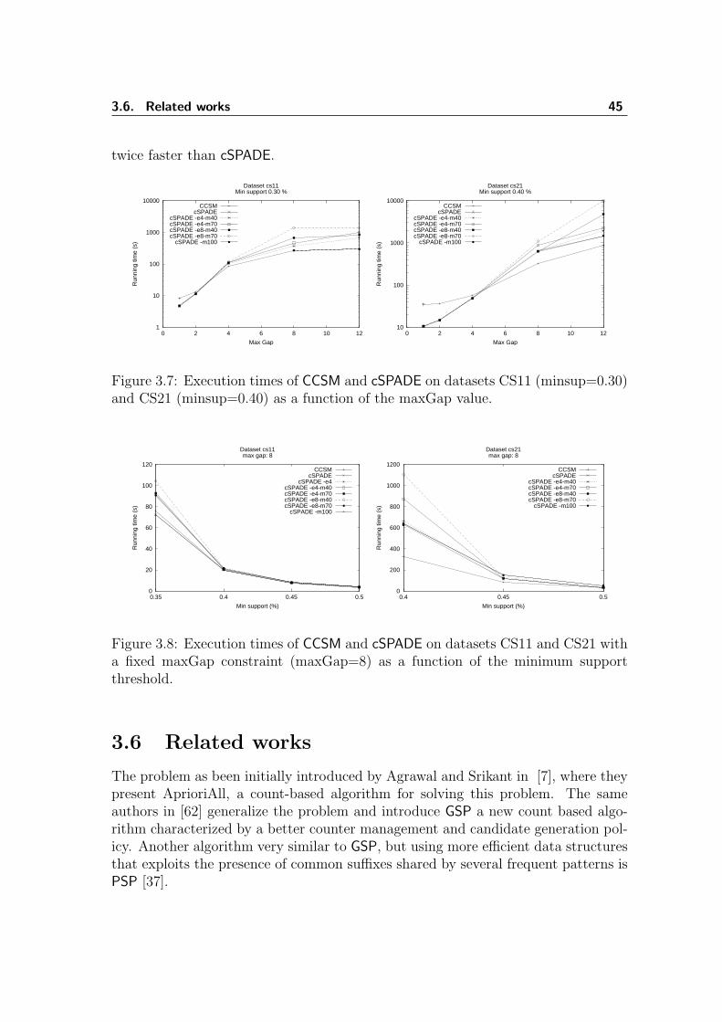
3.6. Related works 45
twice faster than cSPADE.
1
10
100
1000
10000
0 2 4 6 8 10 12
Run
ning
tim
e (s
)
Max Gap
Dataset cs11Min support 0.30 %
CCSMcSPADE
cSPADE -e4-m40cSPADE -e4-m70cSPADE -e8-m40cSPADE -e8-m70
cSPADE -m100
10
100
1000
10000
0 2 4 6 8 10 12
Run
ning
tim
e (s
)
Max Gap
Dataset cs21Min support 0.40 %
CCSMcSPADE
cSPADE -e4-m40cSPADE -e4-m70cSPADE -e8-m40cSPADE -e8-m70
cSPADE -m100
Figure 3.7: Execution times of CCSM and cSPADE on datasets CS11 (minsup=0.30)and CS21 (minsup=0.40) as a function of the maxGap value.
0
20
40
60
80
100
120
0.35 0.4 0.45 0.5
Run
ning
tim
e (s
)
Min support (%)
Dataset cs11max gap: 8
CCSMcSPADE
cSPADE -e4cSPADE -e4-m40cSPADE -e4-m70cSPADE -e8-m40cSPADE -e8-m70
cSPADE -m100
0
200
400
600
800
1000
1200
0.4 0.45 0.5
Run
ning
tim
e (s
)
Min support (%)
Dataset cs21max gap: 8
CCSMcSPADE
cSPADE -e4-m40cSPADE -e4-m70cSPADE -e8-m40cSPADE -e8-m70
cSPADE -m100
Figure 3.8: Execution times of CCSM and cSPADE on datasets CS11 and CS21 witha fixed maxGap constraint (maxGap=8) as a function of the minimum supportthreshold.
3.6 Related works
The problem as been initially introduced by Agrawal and Srikant in [7], where theypresent AprioriAll, a count-based algorithm for solving this problem. The sameauthors in [62] generalize the problem and introduce GSP a new count based algo-rithm characterized by a better counter management and candidate generation pol-icy. Another algorithm very similar to GSP, but using more efficient data structuresthat exploits the presence of common suffixes shared by several frequent patterns isPSP [37].
46 3. Frequent Sequence Mining
As in the association case both intersection based and projection based algo-rithms exists. Two of the best in first category algorithms are SPADE [65, 67, 70],which computes the support of candidates using list intersection and SPAM [8] whichperforms the same operation using vectors of boolean and bitwise operations. Tworepresentatives of the second category are FreeSpan [24] and PrefixSpan [52].
Mannila, Toivonen e Verkamo [35] define a slightly different problem: insteadof frequent patterns common to several input sequences, they search for episodesfrequently appearing in a unique long input sequence. The support for a subsequenceis the number of temporal windows containing it. In a subsequent work [34, 36] thesame authors introduces constraints on single items and pairs of elements presentinside episodes.
Generalizations introduced in GSP [62] are the usage of a taxonomy, the possibil-ity to group together events contained in a specified temporal frame and temporalconstraints on mininum and maximum allowable distance between two consecutiveevents(minGap/maxGap). The proposed algorithm does not handle them efficiently.The performances of SPADE with constraint enforcement (cSPADE [69]) are widelybetter when no constraint is required on maxGap, but are limited as for GSP whenit is enforced. CCSM (S.Orlando,R.Perego,C.Silvestri [46, 47]) have been specificallydesigned in order to overcome his limitation, using a candidate generation methodthat is not affected by maxGap constraint anti-monotonicity. PrefixSpan have beenextended in order to handle several kinds of constraints [53].
A further evolution of PrefixSpan is CloSpan [64], an algorithm that is able todetect all closed sequential patterns2, pruning early during computation most pat-terns that are frequent but not closed. Closed sequential pattern, even if they aremuch more compact, exactly represent the whole set of frequent sequential patternand it is possible to switch from one representation to the other. Nevertheless build-ing the complete set of pattern and checking for inclusion is more expensive than incase of associations. CloSpan was the first algorithm dealing with closed sequentialpattern. More recently, J.Wang and J.Han proposed BIDE a new algorithm thatfind all and only closed patterns, without false positives that need to be correctedwith post processing.
One of the first algorithms for incremental sequence mining is ISM [51] whichuse a method similar to that used by SPADE and in addition maintains the set ofinfrequent candidates(negative border) in order to minimize recomputation. Thisentails a non-trivial resource usage for large datasets, in contrast with ISE [38, 39],which does not need additional data and use just inference from already knownpattern.
2Closed sequential patterns are those sequential patterns that are not contained in any otherpattern having the same support. If B contains A, and both have the same support then everyinput sequence containing A also contains B (the converse is always true).
3.7. Conclusions 47
3.7 Conclusions
In this chapter, we have presented CCSM, a new FSM algorithm that mine temporaldatabases in the presence of user-defined constraints. CCSM searches for sequentialpatterns level-wise, and adopts an intersection-based method to determine the sup-port of candidate k-sequences. Each time a candidate k-sequence α is generated,its support is determined on the fly by joining the k atomic idlists associated withthe frequent items (1-sequences) constituting the candidate. This k-way intersec-tion is, however, a limit case of our method. In fact, our order of generation ofcandidate ensures high locality, so that with high probability successively generatedcandidates share a common subsequence of α. A cache is thus used to store theintermediate idlists associated with all the possible prefixes of α. When the idlistof another candidate β has to be built, we reuse the idlist corresponding to thecommon subsequence of maximal length. The exploitation of such caching strategyentails a strong reduction in the number of join operations actually performed. Fi-nally, CCSM is able to consider the very challenging maxGap constraint over thesequential pattern extracted. Preliminary experiments conducted on syntheticallygenerated datasets showed that CCSM remarkably outperforms cSPADE when theselectivity of the gap constraint is not high. Since we are conscious that furtheroptimization can be pushed into the code, we consider these results as encouraging.
CCSM result sets are strictly ordered on (common part, prefix item, suffix item),thus different result sets can be efficiently merged using a simple list merge. Sincethe distributed and stream FIM algorithms that are presented in the second partof this thesis make a heavy use of result merging, CCSM can be used for efficientlyextending them for solving the FSM problem. In the last chapter, we give somemore detail on this use of CCSM.

48 3. Frequent Sequence Mining

IISecond Part

4Distributed datasets
In many real systems, data are naturally distributed, usually due to a plural owner-ship, or a geographical distribution of the processes that produce the data. Movingall the data to one single location for processing could be impossible due to eitherpolicy or technical reason. Furthermore, the communications between the entitiesowning parts of the data may be not particularly fast and immediate. In this con-text, the communication efficiency of an algorithm is often more important than theexactness of its results.
In this chapter, we will focus on distributed association mining. We will start bycharacterizing the different ways data can be distributed, and describe some usefultechniques common to several distributed association mining algorithms. Then wewill introduce the frequent itemset mining problem for homogeneous distributeddatasets and present two novel communication efficient distributed algorithms forapproximate mining of frequent patterns from transactional databases. Both thealgorithms we propose locally compute frequent patterns, and then merge localresults. The first algorithm, APRed, adaptively reduces the support threshold usedin local computation in order to improve the accuracy of the result, whereas thesecond one, APInterp, uses an effective method for inferring the local support oflocally infrequent itemsets. Both strategies give a good approximation of the set ofthe globally frequent patterns and their supports for sparse datasets, but APInterp
is more resilient to data skew. In the last part of the chapter, we report the resultsof part of the tests we have conducted on publicly available datasets. The goalof these tests is to evaluate the similarity between the exact result set and theapproximate ones returned by our distributed algorithms in different cases, as wellas the scalability of APInterp.
4.1 Introduction
As suggested before, there are several cases in which data can be distributed amongdifferent entities, that we will call nodes. In the case of cellular phone networks,each cell or group of cells may have its separate database for performance andresilience reasons. At the same time other information about the customer thatown a device are available at the account department, and are kept separate due
52 4. Distributed datasets
to privacy reasons. Where a particular data can be found influences the kind ofsolutions a problem can have. Therefore, before describing any algorithm for aparticular data mining problem, we need to specify in which context it will be used.
Homogeneous and heterogeneous data distribution
The two above examples of distributed databases, related to the cellular phonesdomain, fall in two distinct major classes of data distribution. In the first case, eachnode has its own database, containing the log of the activities of a device in the areacontrolled by the group of antennas. Every local database contains different data,but the kind of information is the same for every node. This situation is indicatedas homogeneous data distribution. On the other hand, if we are also interested indata about customers, nodes having different kinds of data need to cooperate. Inthe example, the cell database could contain the information that a device stoppedfor several hours in the same place, whereas the accounting department databaseknows which customer is associated with that device and its home address. Thissituation is indicated as heterogeneous data distribution. In this chapter, we willfocus on association mining on homogeneously distributed data.
Communication bandwidth and latency issues
A key factor in the implementation of distributed algorithms is the kind of com-munication infrastructure available. An algorithm suitable for nodes connected byhigh-speed network links, can be of little use if nodes are connected by a modemand the public telephone network. Furthermore, for an algorithm that entails severalblocking communications, a high latency is definitely a serious issue. Distributedsystems are usually characterized by links having low speed, or high latency, orboth. Hence, efficient algorithms need to exchange as few data as possible, andavoid blocking situation in which the local computation cannot resume until someremote feedback arrives.
Parallel vs Distributed
Parallel (PDM) and distributed (DDM) data-mining are a natural evolution of data-mining technologies, motivated by the need of scalable and high performance sys-tems, or policy/logistic reasons. The main differences between these two approachesis that while in PDM data can be moved (centralized) to a tightly coupled paral-lel system before starting computation, DDM algorithms must deal with limitedpossibilities for data movement/replication, due either to specific policies or techni-cal reasons like large network latencies. A good review of algorithms and issues indistributed data mining is [48].
4.2. Approximated distributed frequent itemset mining 53
4.1.1 Frequent itemset mining
There exists algorithms for distributed frequent itemset mining (FIM) that usuallyperforms in a homogeneous context, and algorithms able to cope with heterogeneousdata, linked by primary keys [27] as, for instance, the individual number in thepreviously seen example about personal data. The two main parallel/distributedapproaches [66], in the homogeneous case, are Count Distribution, in which eachnode computes the support for the same set of candidates on his own dataset, andCandidate/Data Distribution, where each node computes the support of a part ofcandidates, using also part of the dataset owned by other nodes.
More in detail, algorithms based on Count-distribution compute the support ofeach pattern locally, and then exchange (or collect) and sum all the supports toobtain the global support. On the other hand, in Data Distribution and CandidateDistribution each processor handles a disjoint set of candidate patterns, and accessall the data partitions for computing global support. The difference between the twoapproaches is that, in Data Distribution, candidates are partitioned merely to dividethe workload, and all data are accessed by all processors, whereas in CandidateDistribution the candidates are partitioned in such a way that each processor canproceed independently and data are selectively replicated. Since only the countersare sent, Count Distribution minimizes the communications, making it suitable forloosely coupled setting. The other two techniques, instead, are more appropriate forparallel systems.
A first parallel version of Apriori is introduced in [5], while other more efficientsolutions are found in [44, 45, 58, 22, 13, 56, 41, 13, 22, 5, 27, 66]. The diversityof possible use cases makes the selection of the best algorithm a hard task. Evenmetrics used for comparison may be more or less appropriate according to the specificsystem architecture. A good survey on parallel association mining algorithms is [66].
Most these algorithms, however, are not suitable for loosely coupled settings.Only a few papers discussing truly distributed FIM algorithms recently appeared inthe literature [56, 57, 63].
Nevertheless, as previously explained there are several real world systems thatare intrinsically distributed and loosely coupled. For this reason we have chose toprefer DDM solutions, able to deal with such cases.
4.2 Approximated distributed frequent itemset
mining
In this section, we will introduce a novel approximate algorithm for distributedfrequent itemset mining. After a brief summary of the notation used for frequentitemset, we will introduce the centralized algorithm that inspired our algorithmsand its naıve distributed version. Then we will describe APRed and APInterp, thealgorithms we propose, and the experimental results we have obtained. Finally, we
54 4. Distributed datasets
will draw some conclusions.
4.2.1 Overview
A dataset D is a collection of subsets of items I = it1, . . . , itm. Each element of Dis called a transaction. A pattern x is frequent in D with respect to a minimumsupport minsup, if its support is greater than σmin = minsup · |D|, i.e. the patternoccurs in at least σmin transactions, where |D| is the number of transactions in D. Ak-pattern is a pattern composed of k items, Fk is the set of all frequent k-patterns,and F =
⋃iFi is the set of all frequent patterns. F1 is also called the set of frequent
items.In this section, we discuss two distributed algorithms for approximate mining of
frequent itemsets: APRed (Approximate Partition with dynamic minimum supportReduction) and APInterp (Approximate Partition with Interpolation). Both exploitDCI [44], a state-of-the-art algorithm for FIM, as the miner engine used for localcomputations. The name ”Approximate Partition” derives from the distributedcomputation method adopted, which is inspired by the Partition algorithm [55], andits distributed straightforward version [41].
We assume that our dataset D is divided into several disjoint partitions Di, i ={1, ..., n}, located on n collaborating entities, where each transaction completelybelongs to one of the partitions. In particular, we consider that the dataset isalready partitioned, according to some business rules, among geographically dis-tributed systems. Collaborating entities are loosely coupled, and even if availablenetwork bandwidths sometimes is not an issue, latency surely is. A fitting exampleis a set of insurance companies connected by the Internet and collaborate in order todetect frauds. In this kind of setting, we should avoid sending lots of messages withseveral barrier synchronizations. Thus, a small loss of accuracy is a fair trade-off fora reduced number of communications/synchronizations.
Both APRed and APInterp compute independently local solution for each node andthen merge local results. Instead of making a second pass, as Distributed Partitiondoes, we propose other methods to be used during the merge phase in order toimprove the support count. To this end, the minimum support threshold used inlocal computation is adaptively reduced in APRed, whereas an approximate supportinference heuristic is used in APInterp. Experimental tests show that the solutionsproduced by both APRed and APInterp are good approximation of the exact globalresult, and that APInterp is more efficient than APRed. Unfortunately, the APInterp
method may also generate a few false positives, whose approximate supports isusually very close to the exact one. Therefore, the support of the rules extractedfrom these false positive patterns should not bother analysts. This is especially truewhen a positive result just indicate a case that need the attention of the operatorfor further investigation, as in the case of fraud detection: if a pattern with supportslightly higher than the threshold is interesting, probably a slightly lower one willbe interesting too. A single synchronization is required to compute and redistribute
4.2. Approximated distributed frequent itemset mining 55
the reduced support threshold, in APRed, and the knowledge of F2, used by slaves forglobal pruning in both algorithms. This is particularly important in the describeddistributed setting, where the network latency is often a more critical factor thanthe available bandwidth, and the reduced number of communications is worth asmall reduction in the accuracy of results. In APInterp, it is also possible to disablelocal pruning; at the cost of a larger number of false positive, the algorithm becomeasynchronous and suitable for unidirectional communications.
4.2.2 The Distributed Partition algorithm
Our APInterp and APRed algorithms were inspired by Partition [55], a sequential al-gorithm that divides the dataset in several partitions processed independently. Thebasic idea exploited by Partition is the following: each globally frequent pattern mustbe locally frequent in at least one partition. This guarantees that the union of all lo-cal solutions is a superset of the global solution. However, one further pass over thedatabase is necessary to remove all false positives, i.e. patterns that result locallyfrequent but globally infrequent.
Obviously, Partition can be straightforwardly implemented in a distributed set-ting with a master/slave paradigm [41]. Each slave becomes responsible of a localpartition, while the master performs the sum-reduction of local counters (first phase)and orchestrates the slaves for computing the missing local supports for potentiallyglobally frequent patterns (second phase) to remove patterns having global supportless than minsup (false positive patterns collected during the first phase).
While the Distributed Partition algorithm gives the exact values for supports, ithas pros and cons with respect to other distributed algorithms. The pros are re-lated to the number of communications/synchronizations: other methods as count-distribution [22, 68] require several communications/synchronizations, while the Dis-tributed Partition algorithm only requires two communications from the slaves to themaster, one single message from the master to the slaves and one synchronizationafter the first scan. The cons are the size of messages exchanged, and the possibleadditional computation performed by the slaves when the first phase of the algo-rithm produces false positives. Consider that, when low absolute minimum supportsare used, it is likely to produce a lot of false positives due to data skew present inthe various dataset partitions [50]. This has a large impact also on the cost of thesecond phase of the algorithm too: most of the slaves will participate in countingthe local supports of these false positives, thus wasting a lot of time.
One naıve work-around, that we will name Distributed One-pass Partition, consistsin stopping Distributed Partition after the first-pass. So in Distributed One-pass Parti-tion each slave independently computes locally frequent patterns and sends them tothe master which sum-reduces the support for each pattern and writes in the resultset only patterns having the sum of the known supports greater than (or equal to)minsup. Distributed One-pass Partition has obvious performance advantages vs. Dis-tributed Partition. On the other hand, it yields a result that is approximate. Whereas
56 4. Distributed datasets
it is sure that at least the number of occurrences reported in the results exists foreach pattern, it is likely that some pattern has also occurrences in other partitionsin which it was not frequent.
This is formalized in the following lemma.
Lemma 10 (Bounds on support after first pass). Let P=1,...,N be the set of theN partition indexes. Then let fpart(x) = {j ∈ P |σj(x) > minsup · |Dj|} be theset of indexes of the partitions where the pattern x is frequent and let fpart(x) =(P r fpart) be its complement. The support for a pattern x is greater than or equalto the support computed by the Distributed One-pass Partition algorithm:
σ(x)lower =∑
j∈fpart(x)
σj(x)
and is less than or equal to σlower(x) plus the maximum support the same patterncan have in partitions where it is not frequent:
σ(x)upper = σ(x)lower +∑
j∈fpart(x)
minsup · |Dj| − 1
Note that when a pattern does not result frequent in a partition, its actual localsupport can be at most equal to the local minimum support threshold minus one.
We can easily transform the two absolute bounds defined above into the corre-sponding relative ones:
sup(x)upper =σ(x)upper
|D|, sup(x)lower =
σi(x)lower
|D|
These bounds can be used to calculate the Average Support Range described inappendix A (ASR(B), Definition 14). Any approximate algorithm based on Dis-tributed One-pass Partition will yield results with at most this average error on allthe supports.
The main issue with Distributed One-pass Partition is that for every pattern thecomputed support is a very conservative estimate, since it always chooses the lowerbounds to approximate the results. The first method we propose, APRed, aim atincreasing this lower bound. This is obtained by mean of a reduction of the minimumsupport used for local computation in order to increase the probability that globallyfrequent patterns turn out to be locally frequent in most of the dataset partitions.
Generally, any algorithm returning a support value between the bounds willhave better chances of being more accurate. Following this idea, we devised anotheralgorithm based on Distributed One-pass Partition, APInterp, which uses a smart in-terpolation of support. Moreover, it is resilient to skewed item distributions.
4.2. Approximated distributed frequent itemset mining 57
4.2.3 The APRed algorithm
The key idea of APRed, our first approximate FIM algorithm, is to use a slightlyreduced minimum support threshold (an adaptively selected one) for local elabora-tions. The APRed algorithms exploits the same number of communication as thePartition one, and consists of two phases too. The first phase allows the master tocompute a ”good approximation” R′ of R = F1 ∪ F2, where R′ ⊆ R, and a lowerbound σ′(x) for support σ(x) of any patterns x ∈ R. This knowledge of R′ is thenused by each slave for globally pruning the candidates during the second phase. Thisshould reduce the production of false positives on the various slaves. Moreover, atthe end of this first phase, the master also reduces the user-provided minsup, andthis new support threshold is adopted by all the slave for the rest of the computation.The rationale of lowering minsup in local slave computation is to increase the prob-ability that globally frequent patterns turn out to be locally frequent in most of thedataset partitions. Note that when a pattern is locally frequent in all the partitions,the master is able to determine exactly its support. At the end of second phase themaster collects the locally frequent patterns (with respect to the reduced minsup)from the slaves, and simply builds the approximate sets {Fi|i > 2} by summing thesupports associated with corresponding locally frequent patterns. Obviously, evenif the local frequent patterns have been computed by lowering minsup, the masterconsiders a pattern frequent only if this sum is at least |D| ·min supp.The two points to clarify are:
• how the master arrives at a ”good approximation” R′ of R = F1 ∪F2 (at theend of the first phase)
• how the master decides the support reduction ratio r to be used for the restof the computation (during the second phase).
A ”good approximation” for the frequent patterns composed of at most two itemsis built using a significantly reduced minsup for local computation during the firstphase. In our tests, this initial support threshold was set to minsup′ = minsup
2. In
several cases F1 and F2 have much less elements than the following sets Fk, thususing such a low minimum support during the very first part of the computationcould be reasonable for wide ranges of user-specified values of minsup and sparsedatasets. Nevertheless, R′ gives us an accurate knowledge of R = F1∪F2. However,minsup′ is usually too small, and cannot be used for the following iterations.
Before describing the criteria used for deciding the support to use during theremaining iterations, we need to introduce a measure of similarity, which is used tocompare two different result sets A and B. The Sim(A, B) measure, described indetails in Appendix A, ranges from 0 to 1, and considers both false positive/negativeand non-matching support values.
The master chose the new support threshold, minsup′′ ∈ [minsup′, minsup], insuch a way that Sim(R′′, R) is high, where R′′ ⊆ R′ is introduced in the following.
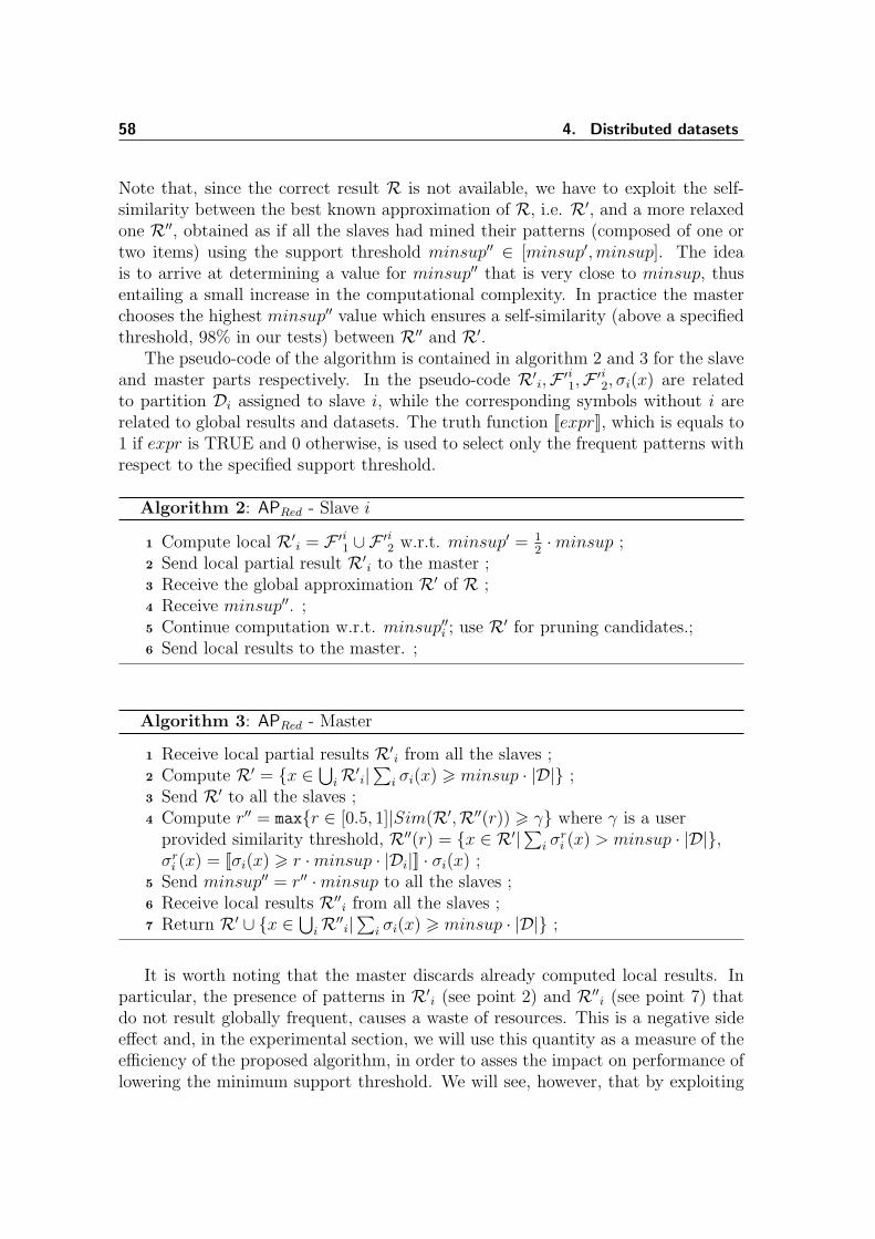
58 4. Distributed datasets
Note that, since the correct result R is not available, we have to exploit the self-similarity between the best known approximation of R, i.e. R′, and a more relaxedone R′′, obtained as if all the slaves had mined their patterns (composed of one ortwo items) using the support threshold minsup′′ ∈ [minsup′, minsup]. The ideais to arrive at determining a value for minsup′′ that is very close to minsup, thusentailing a small increase in the computational complexity. In practice the masterchooses the highest minsup′′ value which ensures a self-similarity (above a specifiedthreshold, 98% in our tests) between R′′ and R′.
The pseudo-code of the algorithm is contained in algorithm 2 and 3 for the slaveand master parts respectively. In the pseudo-code R′
i,F ′i1,F ′i
2, σi(x) are relatedto partition Di assigned to slave i, while the corresponding symbols without i arerelated to global results and datasets. The truth function [[expr]], which is equals to1 if expr is TRUE and 0 otherwise, is used to select only the frequent patterns withrespect to the specified support threshold.
Algorithm 2: APRed - Slave i
Compute local R′i = F ′i
1 ∪ F ′i2 w.r.t. minsup′ = 1
2·minsup ;1
Send local partial result R′i to the master ;2
Receive the global approximation R′ of R ;3
Receive minsup′′. ;4
Continue computation w.r.t. minsup′′i ; use R′ for pruning candidates.;5
Send local results to the master. ;6
Algorithm 3: APRed - Master
Receive local partial results R′i from all the slaves ;1
Compute R′ = {x ∈⋃
iR′i|∑
i σi(x) > minsup · |D|} ;2
Send R′ to all the slaves ;3
Compute r′′ = max{r ∈ [0.5, 1]|Sim(R′,R′′(r)) > γ} where γ is a user4
provided similarity threshold, R′′(r) = {x ∈ R′|∑
i σri (x) > minsup · |D|},
σri (x) = [[σi(x) > r ·minsup · |Di|]] · σi(x) ;
Send minsup′′ = r′′ ·minsup to all the slaves ;5
Receive local results R′′i from all the slaves ;6
Return R′ ∪ {x ∈⋃
iR′′i|∑
i σi(x) > minsup · |D|} ;7
It is worth noting that the master discards already computed local results. Inparticular, the presence of patterns in R′
i (see point 2) and R′′i (see point 7) that
do not result globally frequent, causes a waste of resources. This is a negative sideeffect and, in the experimental section, we will use this quantity as a measure of theefficiency of the proposed algorithm, in order to asses the impact on performance oflowering the minimum support threshold. We will see, however, that by exploiting
4.2. Approximated distributed frequent itemset mining 59
the approximate knowledge R′ of F1 ∪ F2 for candidate pruning we can effectivelyreduce this drawback.
4.2.4 The APInterp algorithm
APInterp, the second distributed algorithm we propose in this chapter, tries to over-come some of the problems encountered by APRed and Distributed One-pass Partitionwhen the data skew between the data partitions is high.
The more evident is that several false positives could be generated, increasingthe resource utilization and the execution time of both Distributed Partition andDistributed One-pass Partition. As APRed, also APInterp addresses this issue by meansof global pruning based on partial knowledge of F2: each locally frequent patternthat contains a globally non-frequent 2-pattern will be locally removed from the setof frequents patterns before sending it to the master and performing next candidategeneration. Moreover this skew might cause a globally frequent pattern x to resultinfrequent on a given partition Di only. In other words, since σi(x) < minsup · |Di|,x will not be returned as a frequent pattern by the ith slave. As a consequence, themaster of Distributed One-pass Partition cannot count on the knowledge of σi(x), andthus cannot exactly compute the global support of x. Unfortunately, in DistributedOne-pass Partition the master might also deduce that x is not globally frequent,because
∑j,j 6=i σj(x) < minsup · |D|.
As explained in the previous section, APRed uses support reduction in order tolimit this issue. Unfortunately, this method exposes APRed to the combinatorialexplosion of the intermediate results, in case the reduced minsup is too small forthe processed dataset. APInterp, instead, allows the master to infer an approximatevalue for this unknown σi(x) by exploiting an interpolation method. The masterbases its interpolation reasoning on the knowledge of:
• the exact support of each single item on all the partitions, and
• the average reduction of the support count of pattern x on all the partitionswhere x resulted actually frequent (and thus returned to the master by theslave), with respect to the support of the least frequent item contained in x:
avg reduct(x) =
∑j∈fpart(x)(
σj(x)
minitem∈x(σj(item)))
|fpart(x)|
where fpart(x) corresponds to the set of data partitions Dj where x actuallyresulted frequent, i.e. where σj(x) ≥ minsup · |Dj|.
The master can thus deduce the unknown support σi(x) on the basis of avg reduct(x)as follows:
σi(x)interp = minitem∈x
(σi(item) ∗ avg reduct(x))
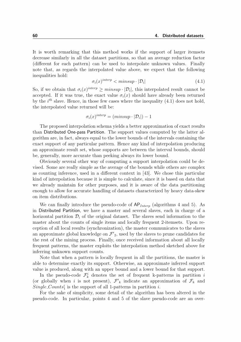
60 4. Distributed datasets
It is worth remarking that this method works if the support of larger itemsetsdecrease similarly in all the dataset partitions, so that an average reduction factor(different for each pattern) can be used to interpolate unknown values. Finallynote that, as regards the interpolated value above, we expect that the followinginequalities hold:
σi(x)interp < minsup · |Di| (4.1)
So, if we obtain that σi(x)interp ≥ minsup · |Di|, this interpolated result cannot beaccepted. If it was true, the exact value σi(x) should have already been returnedby the ith slave. Hence, in those few cases where the inequality (4.1) does not hold,the interpolated value returned will be:
σi(x)interp = (minsup · |Di|)− 1
The proposed interpolation schema yields a better approximation of exact resultsthan Distributed One-pass Partition. The support values computed by the latter al-gorithm are, in fact, always equal to the lower bounds of the intervals containing theexact support of any particular pattern. Hence any kind of interpolation producingan approximate result set, whose supports are between the interval bounds, shouldbe, generally, more accurate than peeking always its lower bound.
Obviously several other way of computing a support interpolation could be de-vised. Some are really simple as the average of the bounds while others are complexas counting inference, used in a different context in [43]. We chose this particularkind of interpolation because it is simple to calculate, since it is based on data thatwe already maintain for other purposes, and it is aware of the data partitioningenough to allow for accurate handling of datasets characterized by heavy data-skewon item distributions.
We can finally introduce the pseudo-code of APInterp (algorithms 4 and 5). Asin Distributed Partition, we have a master and several slaves, each in charge of ahorizontal partition Di of the original dataset. The slaves send information to themaster about the counts of single items and locally frequent 2-itemsets. Upon re-ception of all local results (synchronization), the master communicates to the slavesan approximate global knowledge on F ′
2, used by the slaves to prune candidates forthe rest of the mining process. Finally, once received information about all locallyfrequent patterns, the master exploits the interpolation method sketched above forinferring unknown support counts.
Note that when a pattern is locally frequent in all the partitions, the master isable to determine exactly its support. Otherwise, an approximate inferred supportvalue is produced, along with an upper bound and a lower bound for that support.
In the pseudo-code F ik denotes the set of frequent k-patterns in partition i
(or globally when i is not present), F ′k indicate an approximation of Fk and
Single Countsi1 is the support of all 1-patterns in partition i.
For the sake of simplicity, some detail of the algorithm has been altered in thepseudo-code. In particular, points 4 and 5 of the slave pseudo-code are an over-
4.2. Approximated distributed frequent itemset mining 61
Algorithm 4: APInterp - Slave i
Compute local Single Countsi1 and F i
2. ;1
Send local partial results to the master ;2
Receive the global approximation F ′2 of F2 ;3
Continue computation, by using F ′2 for pruning candidates ;4
Send local results to the master. If computation is over, send an empty5
set ;
Algorithm 5: APInterp - Master
Receive local partial results Single Countsi1 and F i
2 from all the slaves;1
Compute the exact F1, on the basis of the local counts of single items;2
Compute the approximate3
F ′2 = {x ∈
⋃iF i
2 |∑
i counti(x) > minsup · |D|}where if x ∈ F i
2 then counti(x) is equal to σi(x), or is equal to σi(x)interp4
otherwise ;Send F ′
2 to all the slaves ;5
Receive local results from all the slaves (empty for slaves terminated6
before the third iteration) ;Compute and return, for each k, the approximate7
F ′k = {x ∈
⋃iF i
k |∑
i counti(x) > minsup · |D|}8
where if x ∈ F ik then counti(x) is equal to σi(x), or is equal to σi(x)interp
9
otherwise;
62 4. Distributed datasets
simplification of the actual code: pattern are sent, asynchronously, as soon as theyare available in order to optimize communication. Each slave terminates when,at iteration k, less than k + 1 pattern are frequent; this is equivalent to checkingemptiness of F ′i
k+1, but more efficient. On the other side, the master continuouslycollects results from still active slaves and processes them as soon as all expectedresult sets of the same length arrive.
4.2.5 Experimental evaluation
In the following part of the section, we describes the behavior exhibited by ourdistributed approximate algorithms in our experiments. We have run the APRed andAPInterp algorithms on several datasets using different parameters. The goal of thesetests is to understand,
how similarities of the results vary as the minimum support and number ofpartitions change and the scalability.
Similarity and Average Support Range. The method we are proposing yieldsapproximate results. In particular APInterp computes pattern supports which maybe slightly different from the exact ones, thus the result set may miss some frequentpatterns (false negatives) or include some infrequent patterns (false positives). In or-der to evaluate the accuracy of the results we use a widely used measure of similaritybetween two pattern sets introduced in [50], and based on support difference. At thesame time, we have introduced a novel similarity measure, derived from the previousone and used along with it in order to assess the quality of the algorithm output.To the same end, we use the Average support Range (ASR), an intrinsic measure ofthe correctness of the approximation introduced in [61]. An extensive description ofthis measures and a discussion on their use can be found in the appendix A.
Experimental environment
The experiments were performed on a cluster of seven high-end computers, eachequipped with an Intel Xeon 2 GHz, 1 GB of RAM memory and local storage. Inall our tests, we mapped a single process (either master or slave) to each node.This system offers communications with good latency (a dedicated Fast Ethernet).However, since APInterp requires just one synchronization, and all communicationare pipelined, its communication pattern should be suitable even for a distributedsystem characterized by a high latency network.
Experimental data
We performed several tests using datasets from the FIMI’03 contest [1]. We ran-domly partitioned each dataset and used the resulting partitions as input data fordifferent slaves.
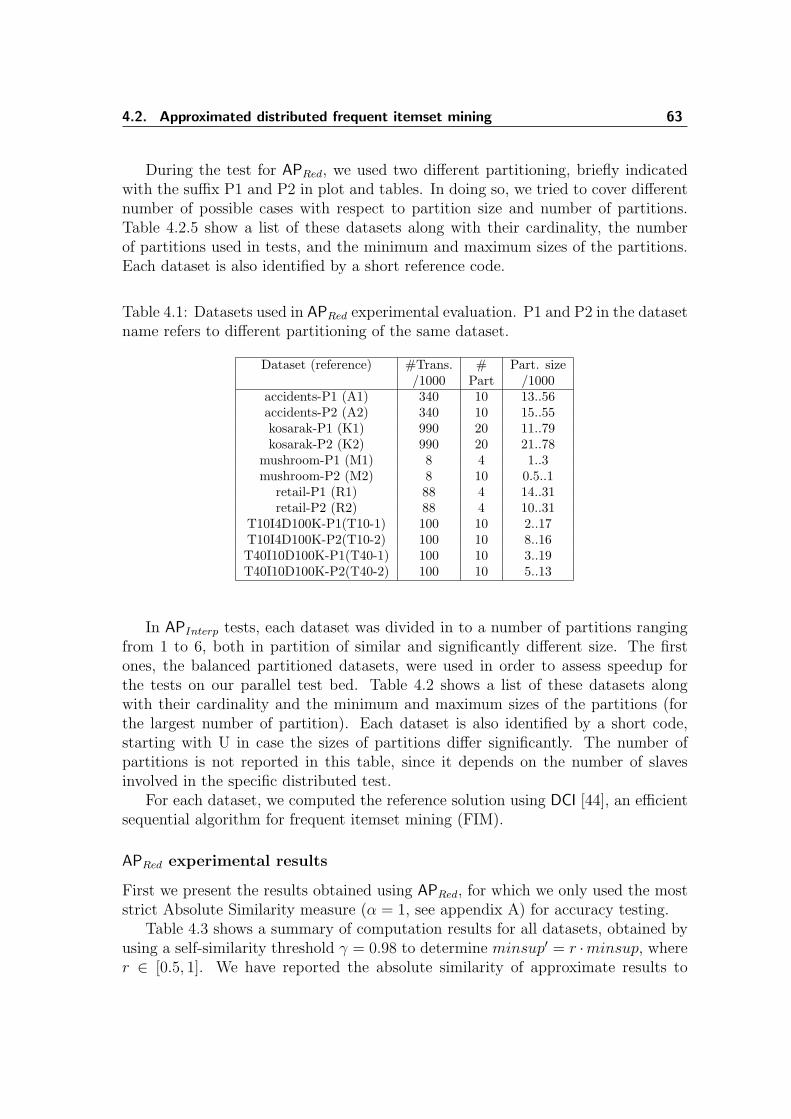
4.2. Approximated distributed frequent itemset mining 63
During the test for APRed, we used two different partitioning, briefly indicatedwith the suffix P1 and P2 in plot and tables. In doing so, we tried to cover differentnumber of possible cases with respect to partition size and number of partitions.Table 4.2.5 show a list of these datasets along with their cardinality, the numberof partitions used in tests, and the minimum and maximum sizes of the partitions.Each dataset is also identified by a short reference code.
Table 4.1: Datasets used in APRed experimental evaluation. P1 and P2 in the datasetname refers to different partitioning of the same dataset.
Dataset (reference) #Trans. # Part. size/1000 Part /1000
accidents-P1 (A1) 340 10 13..56accidents-P2 (A2) 340 10 15..55kosarak-P1 (K1) 990 20 11..79kosarak-P2 (K2) 990 20 21..78
mushroom-P1 (M1) 8 4 1..3mushroom-P2 (M2) 8 10 0.5..1
retail-P1 (R1) 88 4 14..31retail-P2 (R2) 88 4 10..31
T10I4D100K-P1(T10-1) 100 10 2..17T10I4D100K-P2(T10-2) 100 10 8..16T40I10D100K-P1(T40-1) 100 10 3..19T40I10D100K-P2(T40-2) 100 10 5..13
In APInterp tests, each dataset was divided in to a number of partitions rangingfrom 1 to 6, both in partition of similar and significantly different size. The firstones, the balanced partitioned datasets, were used in order to assess speedup forthe tests on our parallel test bed. Table 4.2 shows a list of these datasets alongwith their cardinality and the minimum and maximum sizes of the partitions (forthe largest number of partition). Each dataset is also identified by a short code,starting with U in case the sizes of partitions differ significantly. The number ofpartitions is not reported in this table, since it depends on the number of slavesinvolved in the specific distributed test.
For each dataset, we computed the reference solution using DCI [44], an efficientsequential algorithm for frequent itemset mining (FIM).
APRed experimental results
First we present the results obtained using APRed, for which we only used the moststrict Absolute Similarity measure (α = 1, see appendix A) for accuracy testing.
Table 4.3 shows a summary of computation results for all datasets, obtained byusing a self-similarity threshold γ = 0.98 to determine minsup′ = r ·minsup, wherer ∈ [0.5, 1]. We have reported the absolute similarity of approximate results to
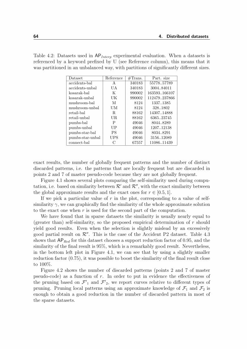
64 4. Distributed datasets
Table 4.2: Datasets used in APInterp experimental evaluation. When a datasets isreferenced by a keyword prefixed by U (see Reference column), this means that itwas partitioned in an unbalanced way, with partitions of significantly different sizes.
Dataset Reference #Trans. Part. sizeaccidents-bal A 340183 55778..57789accidents-unbal UA 340183 3004..84011kosarak-bal K 990002 163593..166107kosarak-unbal UK 990002 112479..237866mushroom-bal M 8124 1337..1385mushroom-unbal UM 8124 328..1802retail-bal R 88162 14307..14888retail-unbal UR 88162 6365..23745pumbs-bal P 49046 8044..8289pumbs-unbal UP 49046 1207..12138pumbs-star-bal PS 49046 8034..8291pumbs-star-unbal UPS 49046 3156..12089connect-bal C 67557 11086..11439
exact results, the number of globally frequent patterns and the number of distinctdiscarded patterns, i.e. the patterns that are locally frequent but are discarded inpoints 2 and 7 of master pseudo-code because they are not globally frequent.
Figure 4.1 shows several plots comparing the self-similarity used during compu-tation, i.e. based on similarity betweenR′ andR′′, with the exact similarity betweenthe global approximate results and the exact ones for r ∈ [0.5, 1].
If we pick a particular value of r in the plot, corresponding to a value of self-similarity γ, we can graphically find the similarity of the whole approximate solutionto the exact one when r is used for the second part of the computation.
We have found that in sparse datasets the similarity is usually nearly equal to(greater than) self-similarity, so the proposed empirical determination of r shouldyield good results. Even when the selection is slightly mislead by an excessivelygood partial result on R′′. This is the case of the Accident P2 dataset. Table 4.3shows that APRed for this dataset chooses a support reduction factor of 0.95, and thesimilarity of the final result is 95%, which is a remarkably good result. Nevertheless,in the bottom left plot in Figure 4.1, we can see that by using a slightly smallerreduction factor (0.75), it was possible to boost the similarity of the final result closeto 100%.
Figure 4.2 shows the number of discarded patterns (points 2 and 7 of masterpseudo-code) as a function of r. In order to put in evidence the effectiveness ofthe pruning based on F ′
1 and F ′2, we report curves relative to different types of
pruning. Pruning local patterns using an approximate knowledge of F1 and F2 isenough to obtain a good reduction in the number of discarded pattern in most ofthe sparse datasets.
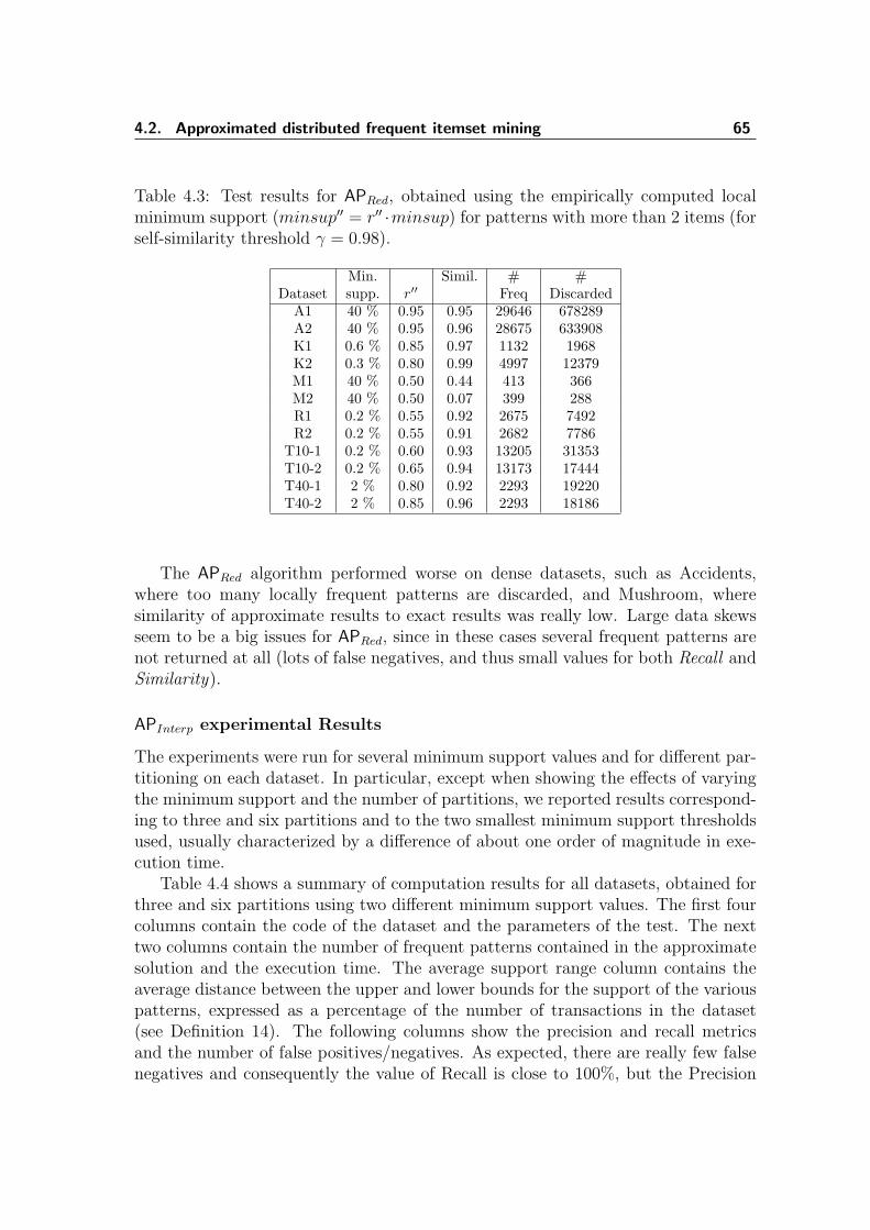
4.2. Approximated distributed frequent itemset mining 65
Table 4.3: Test results for APRed, obtained using the empirically computed localminimum support (minsup′′ = r′′ ·minsup) for patterns with more than 2 items (forself-similarity threshold γ = 0.98).
Min. Simil. # #Dataset supp. r′′ Freq Discarded
A1 40 % 0.95 0.95 29646 678289A2 40 % 0.95 0.96 28675 633908K1 0.6 % 0.85 0.97 1132 1968K2 0.3 % 0.80 0.99 4997 12379M1 40 % 0.50 0.44 413 366M2 40 % 0.50 0.07 399 288R1 0.2 % 0.55 0.92 2675 7492R2 0.2 % 0.55 0.91 2682 7786
T10-1 0.2 % 0.60 0.93 13205 31353T10-2 0.2 % 0.65 0.94 13173 17444T40-1 2 % 0.80 0.92 2293 19220T40-2 2 % 0.85 0.96 2293 18186
The APRed algorithm performed worse on dense datasets, such as Accidents,where too many locally frequent patterns are discarded, and Mushroom, wheresimilarity of approximate results to exact results was really low. Large data skewsseem to be a big issues for APRed, since in these cases several frequent patterns arenot returned at all (lots of false negatives, and thus small values for both Recall andSimilarity).
APInterp experimental Results
The experiments were run for several minimum support values and for different par-titioning on each dataset. In particular, except when showing the effects of varyingthe minimum support and the number of partitions, we reported results correspond-ing to three and six partitions and to the two smallest minimum support thresholdsused, usually characterized by a difference of about one order of magnitude in exe-cution time.
Table 4.4 shows a summary of computation results for all datasets, obtained forthree and six partitions using two different minimum support values. The first fourcolumns contain the code of the dataset and the parameters of the test. The nexttwo columns contain the number of frequent patterns contained in the approximatesolution and the execution time. The average support range column contains theaverage distance between the upper and lower bounds for the support of the variouspatterns, expressed as a percentage of the number of transactions in the dataset(see Definition 14). The following columns show the precision and recall metricsand the number of false positives/negatives. As expected, there are really few falsenegatives and consequently the value of Recall is close to 100%, but the Precision
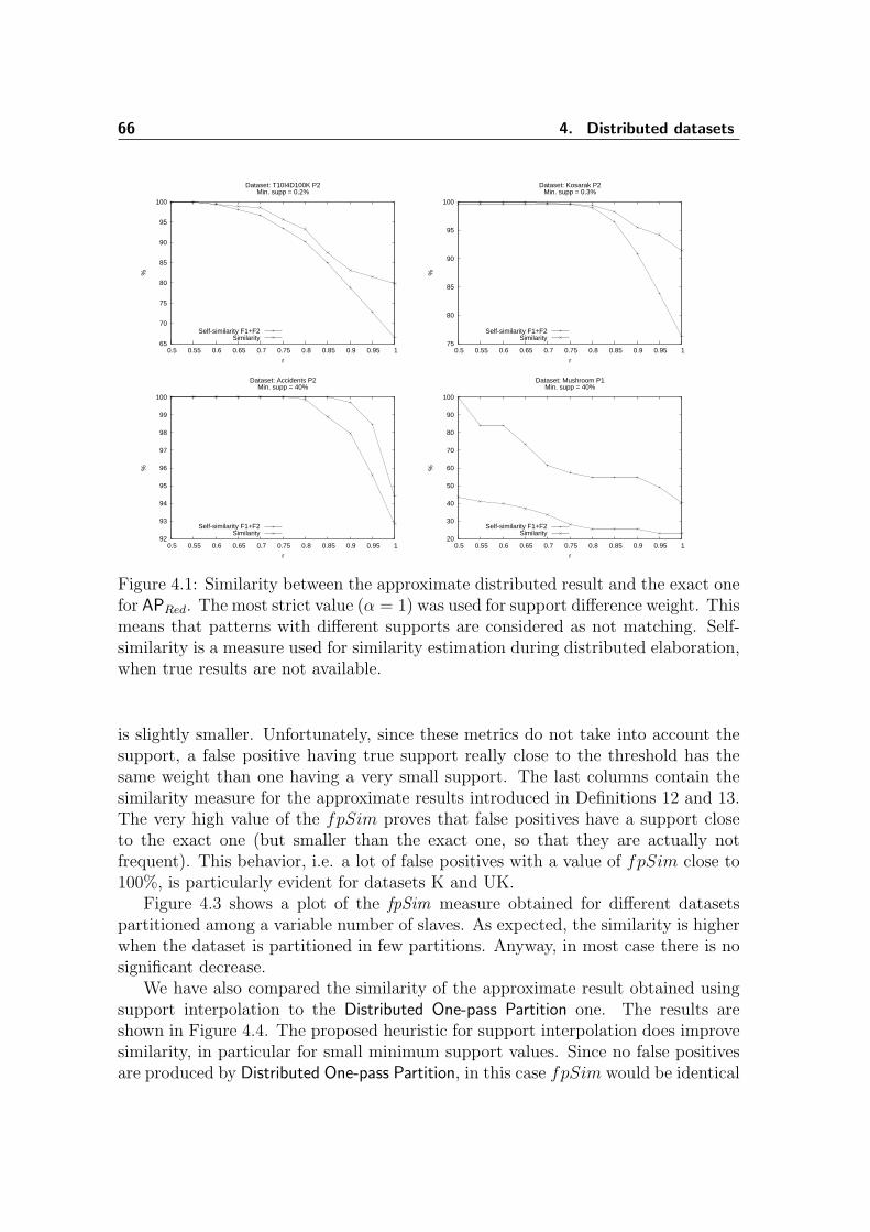
66 4. Distributed datasets
65
70
75
80
85
90
95
100
0.5 0.55 0.6 0.65 0.7 0.75 0.8 0.85 0.9 0.95 1
%
r
Dataset: T10I4D100K P2 Min. supp = 0.2%
Self-similarity F1+F2Similarity
75
80
85
90
95
100
0.5 0.55 0.6 0.65 0.7 0.75 0.8 0.85 0.9 0.95 1
%
r
Dataset: Kosarak P2 Min. supp = 0.3%
Self-similarity F1+F2Similarity
92
93
94
95
96
97
98
99
100
0.5 0.55 0.6 0.65 0.7 0.75 0.8 0.85 0.9 0.95 1
%
r
Dataset: Accidents P2 Min. supp = 40%
Self-similarity F1+F2Similarity
20
30
40
50
60
70
80
90
100
0.5 0.55 0.6 0.65 0.7 0.75 0.8 0.85 0.9 0.95 1
%
r
Dataset: Mushroom P1 Min. supp = 40%
Self-similarity F1+F2Similarity
Figure 4.1: Similarity between the approximate distributed result and the exact onefor APRed. The most strict value (α = 1) was used for support difference weight. Thismeans that patterns with different supports are considered as not matching. Self-similarity is a measure used for similarity estimation during distributed elaboration,when true results are not available.
is slightly smaller. Unfortunately, since these metrics do not take into account thesupport, a false positive having true support really close to the threshold has thesame weight than one having a very small support. The last columns contain thesimilarity measure for the approximate results introduced in Definitions 12 and 13.The very high value of the fpSim proves that false positives have a support closeto the exact one (but smaller than the exact one, so that they are actually notfrequent). This behavior, i.e. a lot of false positives with a value of fpSim close to100%, is particularly evident for datasets K and UK.
Figure 4.3 shows a plot of the fpSim measure obtained for different datasetspartitioned among a variable number of slaves. As expected, the similarity is higherwhen the dataset is partitioned in few partitions. Anyway, in most case there is nosignificant decrease.
We have also compared the similarity of the approximate result obtained usingsupport interpolation to the Distributed One-pass Partition one. The results areshown in Figure 4.4. The proposed heuristic for support interpolation does improvesimilarity, in particular for small minimum support values. Since no false positivesare produced by Distributed One-pass Partition, in this case fpSim would be identical
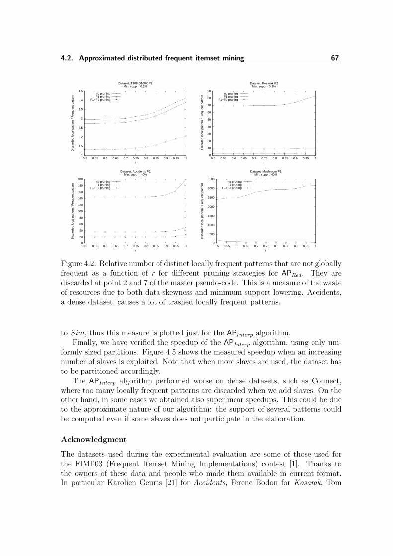
4.2. Approximated distributed frequent itemset mining 67
1
1.5
2
2.5
3
3.5
4
4.5
0.5 0.55 0.6 0.65 0.7 0.75 0.8 0.85 0.9 0.95 1
Dis
card
ed lo
cal p
atte
rn /
Fre
quen
t pat
tern
r
Dataset: T10I4D100K P2 Min. supp = 0.2%
no pruningF1 pruning
F1+F2 pruning
0
10
20
30
40
50
60
70
80
90
0.5 0.55 0.6 0.65 0.7 0.75 0.8 0.85 0.9 0.95 1
Dis
card
ed lo
cal p
atte
rn /
Fre
quen
t pat
tern
r
Dataset: Kosarak P2 Min. supp = 0.3%
no pruningF1 pruning
F1+F2 pruning
0
20
40
60
80
100
120
140
160
180
200
0.5 0.55 0.6 0.65 0.7 0.75 0.8 0.85 0.9 0.95 1
Dis
card
ed lo
cal p
atte
rn /
Fre
quen
t pat
tern
r
Dataset: Accidents P2 Min. supp = 40%
no pruningF1 pruning
F1+F2 pruning
0
500
1000
1500
2000
2500
3000
3500
0.5 0.55 0.6 0.65 0.7 0.75 0.8 0.85 0.9 0.95 1
Dis
card
ed lo
cal p
atte
rn /
Fre
quen
t pat
tern
r
Dataset: Mushroom P1 Min. supp = 40%
no pruningF1 pruning
F1+F2 pruning
Figure 4.2: Relative number of distinct locally frequent patterns that are not globallyfrequent as a function of r for different pruning strategies for APRed. They arediscarded at point 2 and 7 of the master pseudo-code. This is a measure of the wasteof resources due to both data-skewness and minimum support lowering. Accidents,a dense dataset, causes a lot of trashed locally frequent patterns.
to Sim, thus this measure is plotted just for the APInterp algorithm.Finally, we have verified the speedup of the APInterp algorithm, using only uni-
formly sized partitions. Figure 4.5 shows the measured speedup when an increasingnumber of slaves is exploited. Note that when more slaves are used, the dataset hasto be partitioned accordingly.
The APInterp algorithm performed worse on dense datasets, such as Connect,where too many locally frequent patterns are discarded when we add slaves. On theother hand, in some cases we obtained also superlinear speedups. This could be dueto the approximate nature of our algorithm: the support of several patterns couldbe computed even if some slaves does not participate in the elaboration.
Acknowledgment
The datasets used during the experimental evaluation are some of those used forthe FIMI’03 (Frequent Itemset Mining Implementations) contest [1]. Thanks tothe owners of these data and people who made them available in current format.In particular Karolien Geurts [21] for Accidents, Ferenc Bodon for Kosarak, Tom
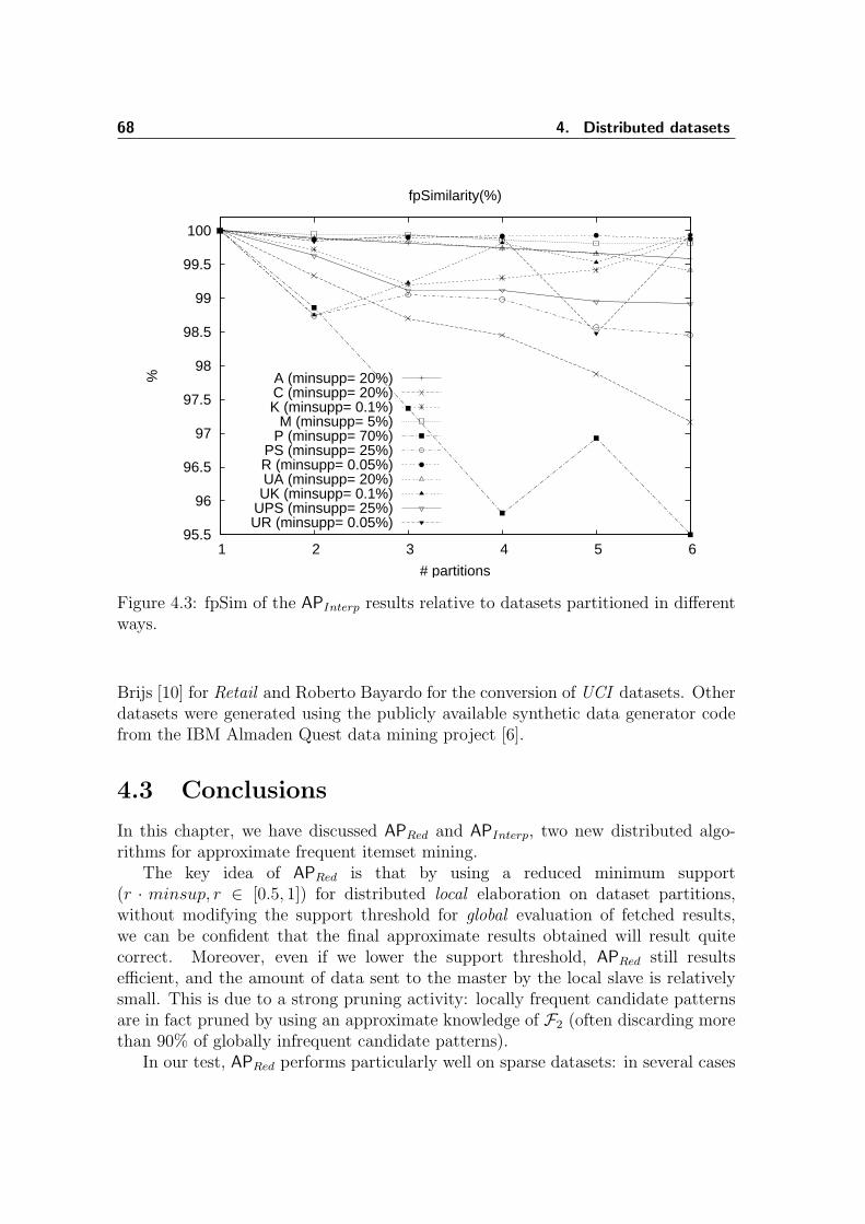
68 4. Distributed datasets
95.5
96
96.5
97
97.5
98
98.5
99
99.5
100
1 2 3 4 5 6
%
# partitions
fpSimilarity(%)
A (minsupp= 20%)C (minsupp= 20%)K (minsupp= 0.1%)
M (minsupp= 5%)P (minsupp= 70%)
PS (minsupp= 25%)R (minsupp= 0.05%)UA (minsupp= 20%)UK (minsupp= 0.1%)
UPS (minsupp= 25%)UR (minsupp= 0.05%)
Figure 4.3: fpSim of the APInterp results relative to datasets partitioned in differentways.
Brijs [10] for Retail and Roberto Bayardo for the conversion of UCI datasets. Otherdatasets were generated using the publicly available synthetic data generator codefrom the IBM Almaden Quest data mining project [6].
4.3 Conclusions
In this chapter, we have discussed APRed and APInterp, two new distributed algo-rithms for approximate frequent itemset mining.
The key idea of APRed is that by using a reduced minimum support(r · minsup, r ∈ [0.5, 1]) for distributed local elaboration on dataset partitions,without modifying the support threshold for global evaluation of fetched results,we can be confident that the final approximate results obtained will result quitecorrect. Moreover, even if we lower the support threshold, APRed still resultsefficient, and the amount of data sent to the master by the local slave is relativelysmall. This is due to a strong pruning activity: locally frequent candidate patternsare in fact pruned by using an approximate knowledge of F2 (often discarding morethan 90% of globally infrequent candidate patterns).
In our test, APRed performs particularly well on sparse datasets: in several cases
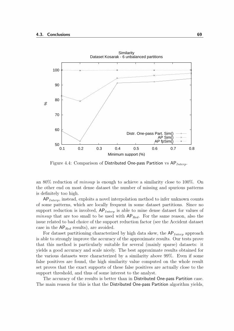
4.3. Conclusions 69
50
60
70
80
90
100
0.1 0.2 0.3 0.4 0.5 0.6 0.7 0.8
%
Minimum support (%)
SimilarityDataset Kosarak - 6 unbalanced partitions
Distr. One-pass Part. Sim()AP Sim()
AP fpSim()
Figure 4.4: Comparison of Distributed One-pass Partition vs APInterp.
an 80% reduction of minsup is enough to achieve a similarity close to 100%. Onthe other end on most dense dataset the number of missing and spurious patternsis definitely too high.
APInterp, instead, exploits a novel interpolation method to infer unknown countsof some patterns, which are locally frequent in some dataset partitions. Since nosupport reduction is involved, APInterp is able to mine dense dataset for values ofminsup that are too small to be used with APRed. For the same reason, also theissue related to bad choice of the support reduction factor (see the Accident datasetcase in the APRed results), are avoided.
For dataset partitioning characterized by high data skew, the APInterp approachis able to strongly improve the accuracy of the approximate results. Our tests provethat this method is particularly suitable for several (mainly sparse) datasets: ityields a good accuracy and scale nicely. The best approximate results obtained forthe various datasets were characterized by a similarity above 99%. Even if somefalse positives are found, the high similarity value computed on the whole resultset proves that the exact supports of these false positives are actually close to thesupport threshold, and thus of some interest to the analyst.
The accuracy of the results is better than in Distributed One-pass Partition case.The main reason for this is that the Distributed One-pass Partition algorithm yields,
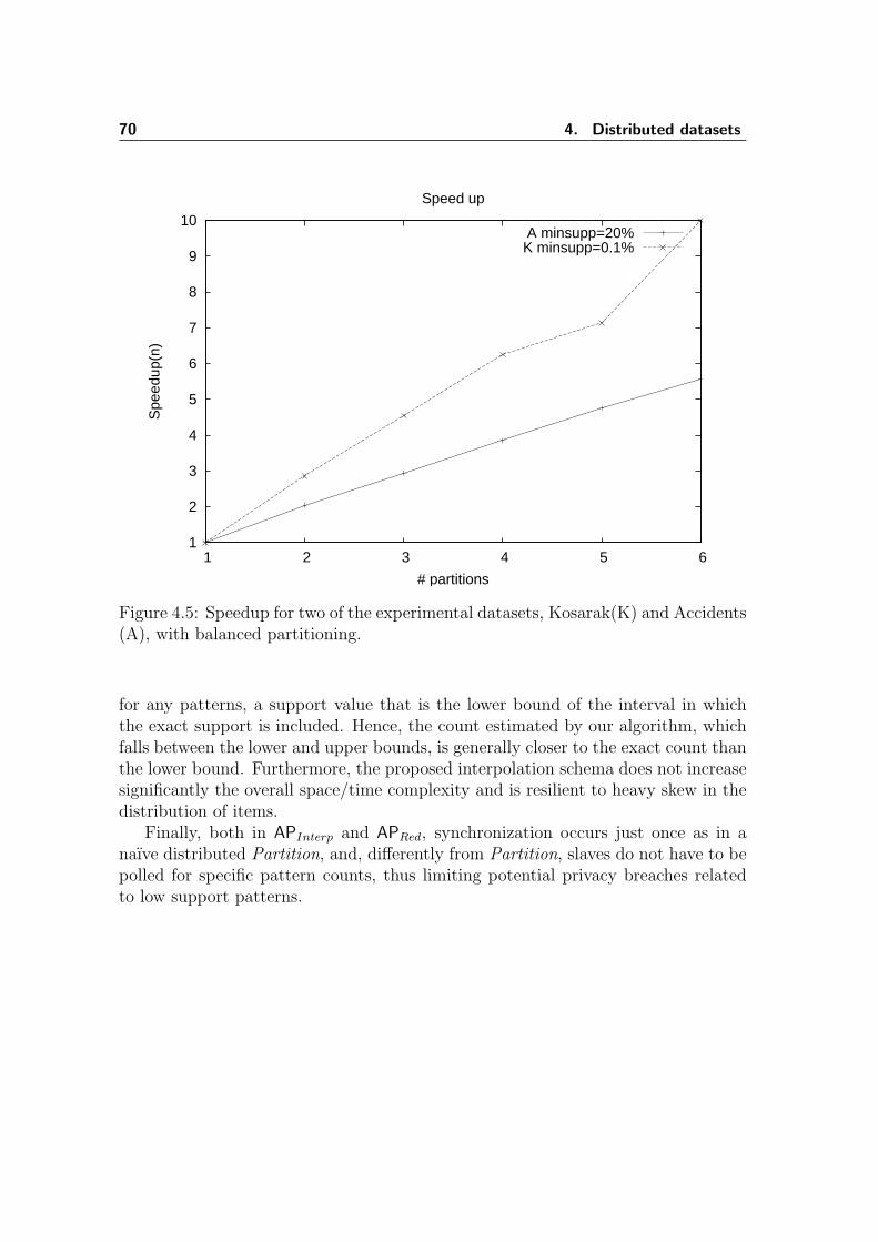
70 4. Distributed datasets
1
2
3
4
5
6
7
8
9
10
1 2 3 4 5 6
Spe
edup
(n)
# partitions
Speed up
A minsupp=20%K minsupp=0.1%
Figure 4.5: Speedup for two of the experimental datasets, Kosarak(K) and Accidents(A), with balanced partitioning.
for any patterns, a support value that is the lower bound of the interval in whichthe exact support is included. Hence, the count estimated by our algorithm, whichfalls between the lower and upper bounds, is generally closer to the exact count thanthe lower bound. Furthermore, the proposed interpolation schema does not increasesignificantly the overall space/time complexity and is resilient to heavy skew in thedistribution of items.
Finally, both in APInterp and APRed, synchronization occurs just once as in anaıve distributed Partition, and, differently from Partition, slaves do not have to bepolled for specific pattern counts, thus limiting potential privacy breaches relatedto low support patterns.
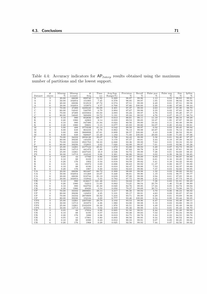
4.3. Conclusions 71
Table 4.4: Accuracy indicators for APInterp results obtained using the maximumnumber of partitions and the lowest support.
# Minsup Minsup # Time Avg.Sup. Precision Recall False pos False neg Sim fpSimDataset slaves % (count) freq (s) Range(%) % % % % % %A 3 20.00 68036 899740 51.92 0.289 98.87 99.96 1.13 0.04 98.83 99.81A 3 30.00 102054 151065 7.45 0.378 98.95 99.97 1.05 0.03 98.92 99.76A 6 20.00 68036 912519 27.72 0.574 97.51 99.99 2.49 0.01 97.51 99.58A 6 30.00 102054 152873 4.57 0.768 97.80 100.00 2.20 0.00 97.80 99.44C 3 70.00 47289 4239440 56.09 2.401 97.37 99.93 2.63 0.07 97.30 98.70C 3 80.00 54045 546795 6.79 2.894 97.67 99.98 2.33 0.02 97.65 98.73C 6 70.00 47289 4335664 93.50 4.093 95.24 99.97 4.76 0.03 95.20 97.17C 6 80.00 54045 560499 10.73 5.191 95.24 99.93 4.76 0.07 95.17 96.74K 3 0.10 990 852636 68.77 0.013 88.81 99.11 11.19 0.89 88.10 99.20K 3 0.20 1980 42963 8.14 0.033 89.53 98.05 10.47 1.95 87.97 98.24K 6 0.10 990 947486 31.94 0.024 80.56 99.89 19.44 0.11 80.49 99.90K 6 0.20 1980 59601 5.15 0.077 65.93 99.80 34.07 0.20 65.84 99.81M 3 5.00 406 3773538 41.14 0.542 99.50 99.97 0.50 0.03 99.45 99.94M 3 8.00 649 864245 8.78 0.862 76.13 99.98 23.87 0.02 76.12 98.62M 6 5.00 406 3888898 67.61 0.899 96.57 100.00 3.43 0.00 96.52 99.81M 6 8.00 649 926827 15.49 1.182 71.00 100.00 29.00 0.00 71.00 97.98P 3 70.00 34332 2858126 39.07 3.766 94.42 99.99 5.58 0.01 94.40 97.37P 3 80.00 39236 145435 2.14 3.170 97.57 99.81 2.43 0.19 97.39 98.52P 6 70.00 34332 2921763 58.23 6.068 92.36 99.99 7.64 0.01 92.34 95.50P 6 80.00 39236 152855 2.62 7.020 92.99 99.97 7.01 0.03 92.96 95.28PS 3 25.00 12261 2177124 29.31 1.672 94.80 99.93 5.20 0.07 94.73 99.05PS 3 30.00 14713 441472 5.80 1.238 97.82 99.78 2.18 0.22 97.61 99.34PS 6 25.00 12261 2227435 45.9 2.526 92.72 99.99 7.28 0.01 92.69 98.45PS 6 30.00 14713 444542 9.06 2.261 96.98 99.61 3.02 0.39 96.59 98.85R 3 0.05 44 17766 0.86 0.005 91.07 99.89 8.93 0.11 90.97 99.90R 3 0.10 88 6105 0.53 0.009 93.39 99.84 6.61 0.16 93.25 99.85R 3 0.20 176 1902 0.34 0.018 94.59 99.82 5.41 0.18 94.42 99.82R 6 0.05 44 18372 0.69 0.006 88.63 99.92 11.37 0.08 88.57 99.88R 6 0.10 88 6190 0.41 0.010 92.47 99.88 7.53 0.12 92.37 99.89R 6 0.20 176 1967 0.30 0.024 92.63 99.96 7.37 0.04 92.60 99.95UA 3 20.00 68036 901687 66.72 0.309 98.68 99.98 1.32 0.02 98.66 99.84UA 3 30.00 102054 151268 10.07 0.440 98.81 99.96 1.19 0.04 98.77 99.77UA 6 20.00 68036 916744 35.19 0.639 97.06 99.99 2.94 0.01 97.05 99.41UA 6 30.00 102054 152942 5.55 0.782 97.75 99.98 2.25 0.02 97.73 99.31UK 3 0.10 990 818017 121.46 0.011 92.62 99.17 7.38 0.83 91.91 99.23UK 3 0.20 1980 52212 11.65 0.062 74.21 98.54 25.79 1.46 73.40 98.89UK 6 0.10 990 922792 45.30 0.020 82.76 99.95 17.24 0.05 82.72 99.94UK 6 0.20 1980 49420 5.54 0.050 79.27 99.69 20.73 0.31 79.08 99.72UP 3 70.00 34332 2800681 38.14 3.217 96.30 99.94 3.70 0.06 96.24 98.02UP 3 80.00 39236 149253 2.25 5.101 95.17 99.91 4.83 0.09 95.07 97.04UP 6 70.00 34332 2879809 56.82 5.216 93.71 99.99 6.29 0.01 93.69 96.66UP 6 80.00 39236 152124 2.69 6.777 93.46 100.00 6.54 0.00 93.44 96.05UPS 3 25.00 12261 2207340 29.79 2.102 93.53 99.96 6.47 0.04 93.48 99.11UPS 3 30.00 14713 455973 6.26 1.980 94.90 99.98 5.10 0.02 94.88 99.19UPS 6 25.00 12261 2162459 44.49 1.976 95.51 99.99 4.49 0.01 95.49 98.92UPS 6 30.00 14713 453334 9.02 2.359 95.46 99.99 4.54 0.01 95.43 98.70UR 3 0.05 44 17654 0.96 0.005 91.56 99.91 8.44 0.09 91.49 99.92UR 3 0.10 88 6185 0.57 0.010 92.48 99.83 7.52 0.17 92.34 99.84UR 3 0.20 176 1896 0.36 0.019 94.75 99.78 5.24 0.22 94.55 99.78UR 6 0.05 44 17901 0.80 0.005 90.56 99.95 9.44 0.05 90.52 99.94UR 6 0.10 88 6390 0.43 0.012 90.33 99.91 9.67 0.09 90.25 99.91UR 6 0.20 176 1968 0.29 0.025 92.56 99.93 7.44 0.07 92.50 99.92

72 4. Distributed datasets
5Streaming data
Many critical applications require a nearly immediate result based on a continuousand infinite stream of data. In our case, we are interested in mining all frequentpatterns and their supports from an infinite stream of transactions. We begin thischapter by describing the peculiarities of streaming data, then we will introducethe problem of finding the most frequent items and itemset in a stream, along withsome state of the art algorithms for solving them. Finally, we will describe ourcontribution: a streaming algorithm for approximate mining of frequent patterns.
5.1 Streaming data
Before introducing the notation used in this chapter, we briefly summarize the no-tation previously used for frequent itemset and frequent items. A dataset D is acollection of subsets of items I = it1, . . . , itm. Each element of D is called a trans-action. A pattern x is frequent in dataset D with respect to a minimum supportminsup, if its support is greater than σmin = minsup · |D|, i.e. the pattern occursin at least σmin transactions, where |D| is the number of transactions in D. A k-pattern is a pattern composed of k items, Fk is the set of all frequent k-patterns,and F =
⋃iFi is the set of all frequent patterns. If D contains just transactions of
one item, then all of the frequent patterns are 1-patterns. These patterns are namedfrequent items.
Since the stream is infinite, new data arrive continuously and results changecontinuously as well. Hence, we need a notation for indicating that a particulardataset or result is referred to a particular time interval. To this end, we write theinterval as a subscript after the entity. Thus D[t0,t1) indicates the part of the streamreceived since t0 and before t1. For the sake of simplicity we will write just D insteadof D[1,t], when referring to all data received until current time t, if this notation isnot ambiguous. As usual, a square bracket indicates that the bound is part of theinterval, whereas a parenthesis indicates that it is excluded.
A pattern x is frequent at time t in the stream D[1,t], with respect to a mini-mum support minsup, if its support is greater than σmin[1,t]
= minsup · |D[1,t]|, i.e.the pattern occurs in at least σmin[1,t]
transactions, where |D[1,t]| is the number oftransactions in the stream D until time t. A k-pattern is a pattern composed of k
74 5. Streaming data
items, Fk[1,t]is the set of all frequent k-patterns, and F[1,t] is the set of all frequent
patterns.
5.1.1 Issues
The infinite nature of these data sources is a serious obstacle to the use of most of thetraditional methods since available computing resources are limited. One of the firsteffects is the need to process data as they arrive. The amount of previously happenedevents is usually overwhelming, so they can be either dropped after processing orarchived separately in secondary storage. In the first case access to past data isobviously impossible whereas in the second case the cost for data retrieval is likelyto be acceptable only for some ”ad hoc” queries, especially when several scan of pastdata are needed to obtain just one single result.
Other important differences with respect to having all data available for the min-ing processed at the same time regard the obtained results. As previously explained,both the data and the results evolve continuously. Hence a result is referred to apart of the stream and, in our case, to the whole part of the stream preceding agiven time t. Obviously, an algorithm suitable for streaming data should be able tocompute the ’next step’ solution on-line, starting from the previously known D[1,t−1)
and the current data D[t−1,t), if necessary with some additional information storedalong with the current solution. In our case, this information is the count of a signif-icant part of frequent single items, and a transaction hash table used for improvingdeterministic bounds on supports returned by the algorithm, as we will explain laterin this chapter.
5.2 Frequent items
Even the apparently simple discovery of frequent items in a stream is challenging,since its exact solution requires to store a counter for each distinct item received.Some items may appear initially in a sporadic way and then become frequent, thusthe only way to exactly compute its support is to maintain a counter since its firstappearance. This could be acceptable when the number of distinct items is reason-ably bounded. If the stream contains a large and potentially unbounded number ofspurious items, as in case of data with probabilities of occurrence that follows Zipf’slaw like internet traffic data, this approach may lead to a huge waste of memory.Furthermore, the number of distinct items is potentially proportional to the lengthof the stream. The Top Frequent items problem is closely related to the frequentitems one, except that the user does not directly decide the support threshold: theresult set contains only a given number of items having the highest supports. In thiscase too the resource usage is unbounded. This issue has been addressed by severalapproximate algorithms, which sacrifice the exactness of the result in order to limitthe space complexity. In this section, we will formally introduce the problem, and
5.2. Frequent items 75
then we will describe some representative approximate algorithms for finding the setof most frequent items.
5.2.1 Problem
Let D[1,n] = s1, s2, . . . , sn be a data stream, where each position in the stream si
contains an element of the items I = it1, . . . , itm. Let item iti occur σ[1,n](iti) timesin D[1,n]. The k items having the highest frequencies are named the top-k itemswhereas items whose frequencies are greater than σmin = minsup · |D| are namedfrequent items.
As explained before and in [12] the exact solution of this problem is a highlymemory intensive problem. Two relaxed versions of this problem have been intro-duced in [12]: FindCandidateTop(S, k, l) and FindApproxTop(S, k, ε). Thefirst one is exact and consists in finding a list of l items containing the k mostfrequent, whereas the second one is approximate. Its goal is to find a list of itemshaving a frequency greater than (1− ε) ·σ[1,n](itk) where itk is the kth most frequentitem. FindCandidateTop can be very hard to solve for some input distributions,in particular when the frequencies of the kth and the (l + 1)th are similar. In suchcases, the approximate problem is more practical to solve. Several variation of thetop-k frequent items problem have been proposed. The Hot Items problem describedin [40] for large datasets and, several year after, adapted to data streams ([16, 30])is essentially the top-k frequent items problem formalized in a slightly different way.
The techniques used for solving this family of problems can be classified into twolarge categories: count-based techniques and sketch-based techniques. The first onesmonitor a limited set of potentially ”interesting” items, using a counter for each oneof them. In this case, an error arise when an item is erroneously kept out of the setor inserted too late. The second family provides a frequency estimation for everyitem by using a hash-indexed vector of counters. In this case, the risk of completelymissing the occurrences of an item is avoided, at the cost of looser guarantees onthe computed frequencies.
5.2.2 Count-based algorithms
Count-based algorithms maintains a set of counters, each one associated with aspecific item. When the number of distinct items is supposed to be high, therecould be not enough memory for allocating all the counters. In this case, it isnecessary to limit our attention to a set of items compatible with the availablememory. Only the items in the monitored set have an associated counter, which isincremented upon their arrival. Other items have just an opportunity to replace oneof the monitored items. In fact, in most methods, the set of monitored items variesduring the computation. Each algorithm of this family is characterized by the datastructure for the efficient maintenance of counters and the policy for replacing ”old”counters it uses.
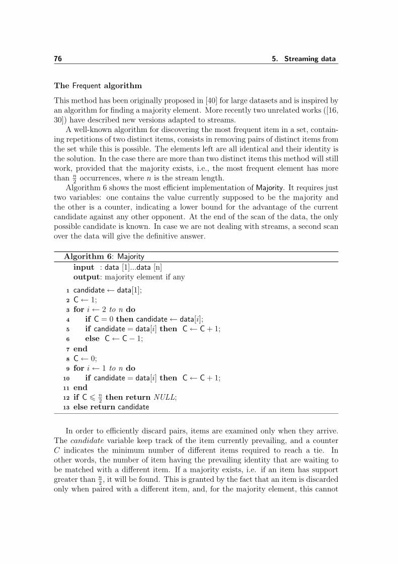
76 5. Streaming data
The Frequent algorithm
This method has been originally proposed in [40] for large datasets and is inspired byan algorithm for finding a majority element. More recently two unrelated works ([16,30]) have described new versions adapted to streams.
A well-known algorithm for discovering the most frequent item in a set, contain-ing repetitions of two distinct items, consists in removing pairs of distinct items fromthe set while this is possible. The elements left are all identical and their identity isthe solution. In the case there are more than two distinct items this method will stillwork, provided that the majority exists, i.e., the most frequent element has morethan n
2occurrences, where n is the stream length.
Algorithm 6 shows the most efficient implementation of Majority. It requires justtwo variables: one contains the value currently supposed to be the majority andthe other is a counter, indicating a lower bound for the advantage of the currentcandidate against any other opponent. At the end of the scan of the data, the onlypossible candidate is known. In case we are not dealing with streams, a second scanover the data will give the definitive answer.
Algorithm 6: Majority
input : data [1]...data [n]output: majority element if any
candidate← data[1];1
C← 1;2
for i← 2 to n do3
if C = 0 then candidate← data[i];4
if candidate = data[i] then C← C + 1;5
else C← C− 1;6
end7
C← 0;8
for i← 1 to n do9
if candidate = data[i] then C← C + 1;10
end11
if C 6 n2
then return NULL;12
else return candidate13
In order to efficiently discard pairs, items are examined only when they arrive.The candidate variable keep track of the item currently prevailing, and a counterC indicates the minimum number of different items required to reach a tie. Inother words, the number of item having the prevailing identity that are waiting tobe matched with a different item. If a majority exists, i.e. if an item has supportgreater than n
2, it will be found. This is granted by the fact that an item is discarded
only when paired with a different item, and, for the majority element, this cannot
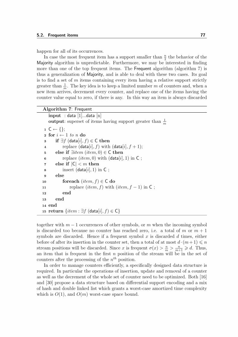
5.2. Frequent items 77
happen for all of its occurrences.In case the most frequent item has a support smaller than n
2the behavior of the
Majority algorithm is unpredictable. Furthermore, we may be interested in findingmore than one of the top frequent items. The Frequent algorithm (algorithm 7) isthus a generalization of Majority, and is able to deal with these two cases. Its goalis to find a set of m items containing every item having a relative support strictlygreater than 1
m. The key idea is to keep a limited number m of counters and, when a
new item arrives, decrement every counter, and replace one of the items having thecounter value equal to zero, if there is any. In this way an item is always discarded
Algorithm 7: Frequent
input : data [1]...data [n]output: superset of items having support greater than 1
m
C← {};1
for i← 1 to n do2
if ∃f (data[i], f) ∈ C then3
replace (data[i], f) with (data[i], f + 1);4
else if ∃item (item, 0) ∈ C then5
replace (item, 0) with (data[i], 1) in C ;6
else if |C| < m then7
insert (data[i], 1) in C ;8
else9
foreach (item, f) ∈ C do10
replace (item, f) with (item, f − 1) in C ;11
end12
end13
end14
return {item : ∃f (data[i], f) ∈ C}15
together with m− 1 occurrences of other symbols, or m when the incoming symbolis discarded too because no counter has reached zero, i.e. a total of m or m + 1symbols are discarded. Hence if a frequent symbol x is discarded d times, eitherbefore of after its insertion in the counter set, then a total of at most d · (m+1) 6 nstream positions will be discarded. Since x is frequent σ(x) > n
m> n
m+1> d. Thus,
an item that is frequent in the first n position of the stream will be in the set ofcounters after the processing of the nth position.
In order to manage counters efficiently, a specifically designed data structure isrequired. In particular the operations of insertion, update and removal of a counteras well as the decrement of the whole set of counter need to be optimized. Both [16]and [30] propose a data structure based on differential support encoding and a mixof hash and double linked list which grants a worst-case amortized time complexitywhich is O(1), and O(m) worst-case space bound.
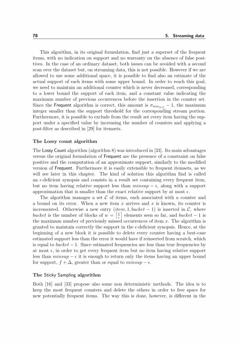
78 5. Streaming data
This algorithm, in its original formulation, find just a superset of the frequentitems, with no indication on support and no warranty on the absence of false posi-tives. In the case of an ordinary dataset, both issues can be avoided with a secondscan over the dataset but, on streaming data, this is not possible. However if we areallowed to use some additional space, it is possible to find also an estimate of theactual support of each items with some upper bound. In order to reach this goal,we need to maintain an additional counter which is never decreased, correspondingto a lower bound the support of each item, and a constant value indicating themaximum number of previous occurrences before the insertion in the counter set.Since the Frequent algorithm is correct, this amount is σmin[1,t]
− 1, the maximuminteger smaller than the support threshold for the corresponding stream portion.Furthermore, it is possible to exclude from the result set every item having the sup-port under a specified value by increasing the number of counters and applying apost-filter as described in [29] for itemsets.
The Lossy count algorithm
The Lossy Count algorithm (algorithm 8) was introduced in [33]. Its main advantagesversus the original formulation of Frequent are the presence of a constraint on falsepositive and the computation of an approximate support, similarly to the modifiedversion of Frequent. Furthermore it is easily extensible to frequent itemsets, as wewill see later in this chapter. The kind of solution this algorithm find is calledan ε-deficient synopsis and consists in a result set containing every frequent item,but no item having relative support less than minsup − ε, along with a supportapproximation that is smaller than the exact relative support by at most ε.
The algorithm manages a set C of items, each associated with a counter anda bound on its error. When a new item x arrives and x is known, its counter isincremented. Otherwise a new entry (item, 1, bucket − 1) is inserted in C, wherebucket is the number of blocks of w =
⌈1ε
⌉elements seen so far, and bucket − 1 is
the maximum number of previously missed occurrences of item x. The algorithm isgranted to maintain correctly the support in the ε-deficient synopsis. Hence, at thebeginning of a new block it is possible to delete every counter having a best-caseestimated support less than the error it would have if reinserted from scratch, whichis equal to bucket− 1. Since estimated frequencies are less than true frequencies byat most ε, in order to get every frequent item but no item having relative supportless than minsup − ε it is enough to return only the items having an upper boundfor support, f + ∆, greater than or equal to minsup− ε.
The Sticky Sampling algorithm
Both [16] and [33] propose also some non deterministic methods. The idea is tokeep the most frequent counters and delete the others in order to free space fornew potentially frequent items. The way this is done, however, is different in the
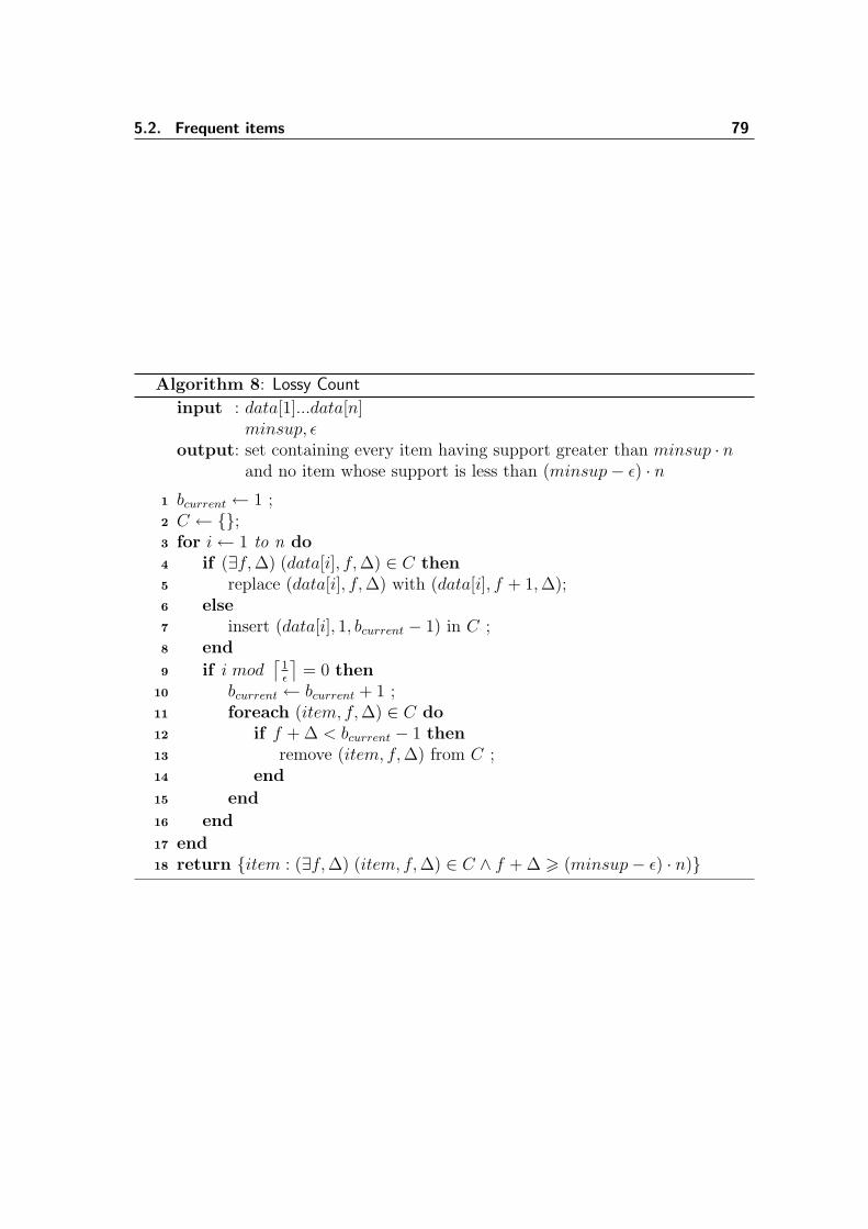
5.2. Frequent items 79
Algorithm 8: Lossy Count
input : data[1]...data[n]minsup, ε
output: set containing every item having support greater than minsup · nand no item whose support is less than (minsup− ε) · n
bcurrent ← 1 ;1
C ← {};2
for i← 1 to n do3
if (∃f, ∆) (data[i], f, ∆) ∈ C then4
replace (data[i], f, ∆) with (data[i], f + 1, ∆);5
else6
insert (data[i], 1, bcurrent − 1) in C ;7
end8
if i mod⌈
1ε
⌉= 0 then9
bcurrent ← bcurrent + 1 ;10
foreach (item, f, ∆) ∈ C do11
if f + ∆ < bcurrent − 1 then12
remove (item, f, ∆) from C ;13
end14
end15
end16
end17
return {item : (∃f, ∆) (item, f, ∆) ∈ C ∧ f + ∆ > (minsup− ε) · n)}18
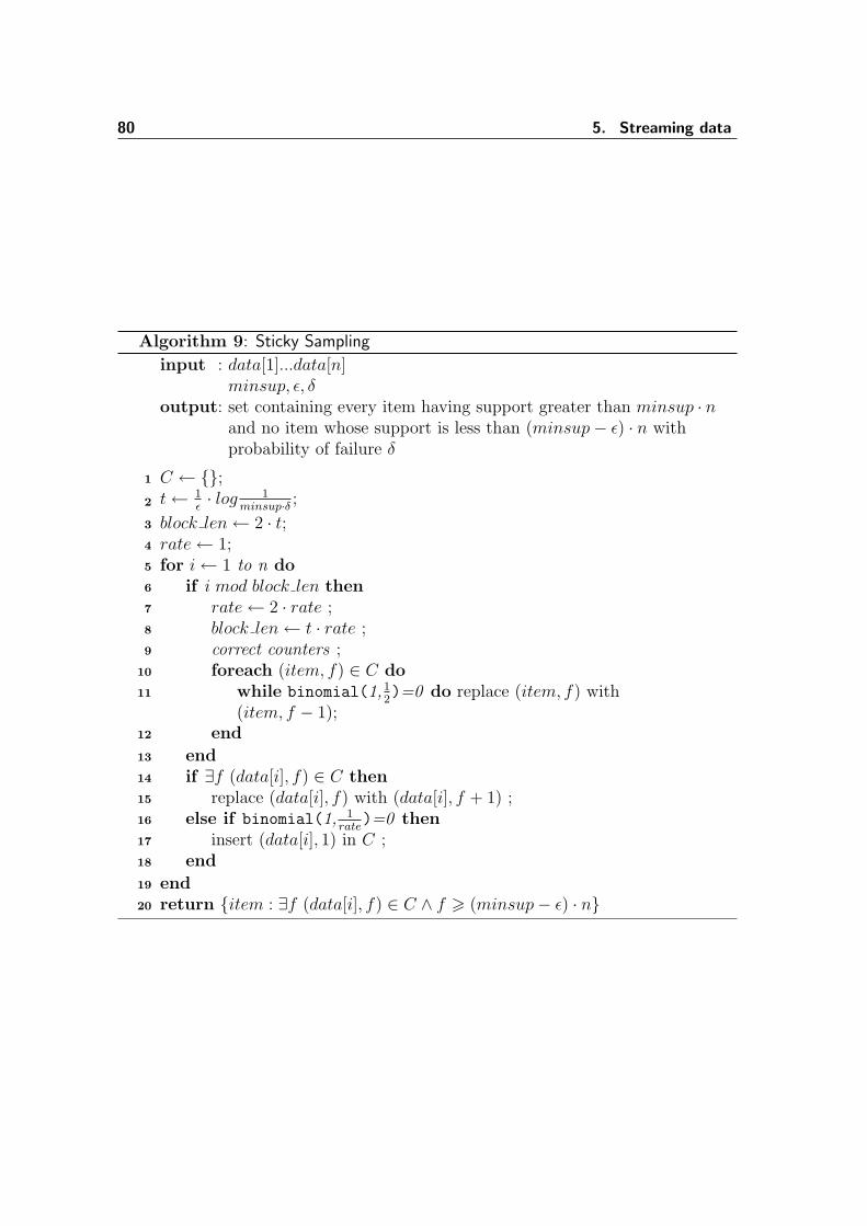
80 5. Streaming data
Algorithm 9: Sticky Sampling
input : data[1]...data[n]minsup, ε, δ
output: set containing every item having support greater than minsup · nand no item whose support is less than (minsup− ε) · n withprobability of failure δ
C ← {};1
t← 1ε· log 1
minsup·δ ;2
block len← 2 · t;3
rate← 1;4
for i← 1 to n do5
if i mod block len then6
rate← 2 · rate ;7
block len← t · rate ;8
correct counters ;9
foreach (item, f) ∈ C do10
while binomial(1,12)=0 do replace (item, f) with11
(item, f − 1);end12
end13
if ∃f (data[i], f) ∈ C then14
replace (data[i], f) with (data[i], f + 1) ;15
else if binomial(1, 1rate
)=0 then16
insert (data[i], 1) in C ;17
end18
end19
return {item : ∃f (data[i], f) ∈ C ∧ f > (minsup− ε) · n}20
5.2. Frequent items 81
two cases. Probabilistic-Inplace [16] discard one-half of the counters every r receiveditems and select the first items found immediately after the discard occurs. StickySampling [33] (algorithm 9) use, instead, a uniform sampling strategy over the wholestream. In order to keep the number of counters probabilistically bounded, thesampling rate is decreased for increasing stream lengths, and the previously knownfrequencies are corrected to reflect the new rate using a stochastic method.
5.2.3 Sketch-based algorithms
As Count-based algorithms, also Sketch-based ones maintain a set of counters but,instead of associating the counters with particular items, they are associated withdifferent overlapping groups of items. The analysis of the values of the counters forthe various groups containing an item allows us to give an estimate of its support.In this approach there is no notion of monitored item, and the support estimationis possible for any item. Algorithms included in this family, as in the case of theCount-based family, share the same basic skeleton. The main differences are inthe management of the counters, the kind of other queries that can be answeredby using the same count-sketch and the exact function used for support estimation,which directly influence the space requirements based on the user selected acceptableerror probability. In [15] G.Cormode and S.Muthukrishnan present their particularlyflexible Count-Min Sketch data structure as well as a good comparison to other stateof the art sketch techniques. We will adopt their unification framework in order todescribe a generic sketch based algorithm.
A sketch is a two dimensional array of dimension w by d. Let m be the numberof distinct items, h1 . . . hd be hash functions mapping {1 . . . m} into {1 . . . w} andlet g1 . . . gd be other hash functions defined on items. The (j, k) entry of the sketchis defined to be ∑
i:hk(i)=j
σ(i) · gk(i)
In other words, when an item i arrives, for each k ∈ {1 . . . d} the entry (hk(i), k)is increased by the amount gk(i), which is algorithm dependent. Thus, the updatetime complexity is O(d) and the space complexity is O(wd), provided that the hashfunctions can be stored efficiently. The way the data structure is used in order toanswer a particular query, the required randomness and independence of the hashfunctions, as well as the minimum size of the sketch array needed to guarantee thefulfillment of probability of error constraints, are algorithm dependent.
A particularly simple count sketch is Count-Min [15]. In its case the values offunctions gk(item) are always 1, i.e. each counter is incremented by one each timean item is transformed into its identifier by a hash function. The approximate valueis computed as the smallest of the counters associated with an item by any hashfunction. Since several items can be hashed to the same integer, the approximatevalue is always greater than the exact one. The two fragments of pseudo-code show
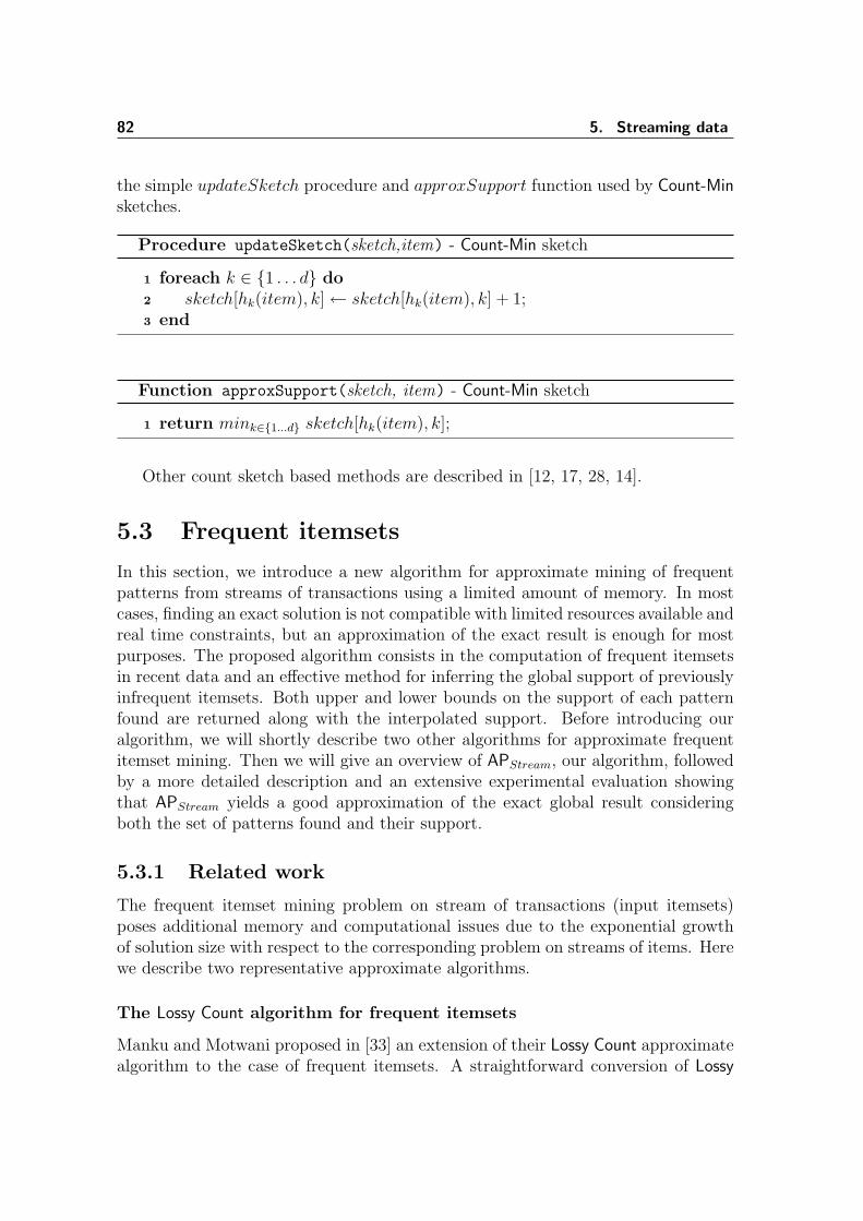
82 5. Streaming data
the simple updateSketch procedure and approxSupport function used by Count-Minsketches.
Procedure updateSketch(sketch,item) - Count-Min sketch
foreach k ∈ {1 . . . d} do1
sketch[hk(item), k]← sketch[hk(item), k] + 1;2
end3
Function approxSupport(sketch, item) - Count-Min sketch
return mink∈{1...d} sketch[hk(item), k];1
Other count sketch based methods are described in [12, 17, 28, 14].
5.3 Frequent itemsets
In this section, we introduce a new algorithm for approximate mining of frequentpatterns from streams of transactions using a limited amount of memory. In mostcases, finding an exact solution is not compatible with limited resources available andreal time constraints, but an approximation of the exact result is enough for mostpurposes. The proposed algorithm consists in the computation of frequent itemsetsin recent data and an effective method for inferring the global support of previouslyinfrequent itemsets. Both upper and lower bounds on the support of each patternfound are returned along with the interpolated support. Before introducing ouralgorithm, we will shortly describe two other algorithms for approximate frequentitemset mining. Then we will give an overview of APStream, our algorithm, followedby a more detailed description and an extensive experimental evaluation showingthat APStream yields a good approximation of the exact global result consideringboth the set of patterns found and their support.
5.3.1 Related work
The frequent itemset mining problem on stream of transactions (input itemsets)poses additional memory and computational issues due to the exponential growthof solution size with respect to the corresponding problem on streams of items. Herewe describe two representative approximate algorithms.
The Lossy Count algorithm for frequent itemsets
Manku and Motwani proposed in [33] an extension of their Lossy Count approximatealgorithm to the case of frequent itemsets. A straightforward conversion of Lossy
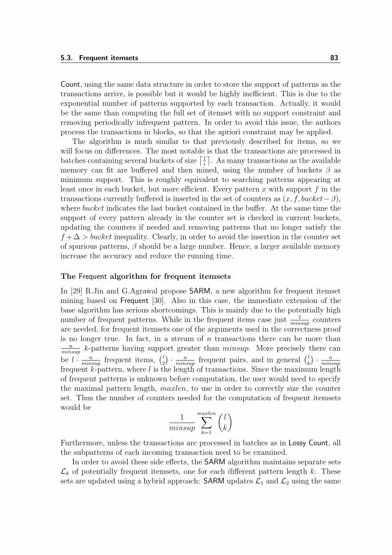
5.3. Frequent itemsets 83
Count, using the same data structure in order to store the support of patterns as thetransactions arrive, is possible but it would be highly inefficient. This is due to theexponential number of patterns supported by each transaction. Actually, it wouldbe the same than computing the full set of itemset with no support constraint andremoving periodically infrequent pattern. In order to avoid this issue, the authorsprocess the transactions in blocks, so that the apriori constraint may be applied.
The algorithm is much similar to that previously described for items, so wewill focus on differences. The most notable is that the transactions are processed inbatches containing several buckets of size
⌈1ε
⌉. As many transactions as the available
memory can fit are buffered and then mined, using the number of buckets β asminimum support. This is roughly equivalent to searching patterns appearing atleast once in each bucket, but more efficient. Every pattern x with support f in thetransactions currently buffered is inserted in the set of counters as (x, f, bucket−β),where bucket indicates the last bucket contained in the buffer. At the same time thesupport of every pattern already in the counter set is checked in current buckets,updating the counters if needed and removing patterns that no longer satisfy thef +∆ > bucket inequality. Clearly, in order to avoid the insertion in the counter setof spurious patterns, β should be a large number. Hence, a larger available memoryincrease the accuracy and reduce the running time.
The Frequent algorithm for frequent itemsets
In [29] R.Jin and G.Agrawal propose SARM, a new algorithm for frequent itemsetmining based on Frequent [30]. Also in this case, the immediate extension of thebase algorithm has serious shortcomings. This is mainly due to the potentially highnumber of frequent patterns. While in the frequent items case just 1
minsupcounters
are needed, for frequent itemsets one of the arguments used in the correctness proofis no longer true. In fact, in a stream of n transactions there can be more than
nminsup
k-patterns having support greater than minsup. More precisely there can
be l · nminsup
frequent items,(
l2
)· n
minsupfrequent pairs, and in general
(lk
)· n
minsup
frequent k-pattern, where l is the length of transactions. Since the maximum lengthof frequent patterns is unknown before computation, the user would need to specifythe maximal pattern length, maxlen, to use in order to correctly size the counterset. Thus the number of counters needed for the computation of frequent itemsetswould be
1
minsup
maxlen∑k=1
(l
k
)Furthermore, unless the transactions are processed in batches as in Lossy Count, allthe subpatterns of each incoming transaction need to be examined.
In order to avoid these side effects, the SARM algorithm maintains separate setsLk of potentially frequent itemsets, one for each different pattern length k. Thesesets are updated using a hybrid approach: SARM updates L1 and L2 using the same
84 5. Streaming data
method proposed in Frequent, and at the same time buffers transactions for a level-wise batched processing. When a transaction t arrives, it is inserted in a buffer, andboth L1 and L2 are updated either by incrementing the count, for already knownpatterns, or inserting the new ones. If the size of L2 exceeds the limit f · 1
minsup·ε ,
where ε ∈ [0, 1] is a factor used for increasing the accuracy, and f is the averagenumber of 2-patterns per transaction, then the size of L2 is reduced by executingthe CrossOver operation, consisting in decreasing every counter and removing, asin Frequent, patterns having count equal to zero. Every time this operation isperformed, the transaction buffer is processed. For increasing values of k > 2, thek-patterns appearing in the buffer and having all subpatterns included in Lk−1 areused for updating Lk. Then the buffer is emptied and the CrossOver operation isapplied to each Lk.
The ε ∈ [0, 1] factor can be used for enforcing a bound on result accuracy. If ε < 1then no itemset having relative support less than (1−ε) ·minsup will be in the resultset. Thus Fminsup ⊆ L ⊆ F (1−ε)·minsup, where L is the result set, and F s is the set ofitemset whose support exceed s. When ε = 1 the SARM algorithm is not able to giveany guarantee on the accuracy, as the Frequent algorithm. Furthermore, both LossyCount for itemsets and SARM ignore previous potential occurrences of a patternwhen it is inserted into the set of frequent patterns. In the case of Lossy Count themaximum number of neglected occurrences is returned along with the support, butno other information available during the stream processing is exploited.
5.3.2 The APStream algorithm
In order to overcome these limitations APStream (Approximate Partition for Stream),the algorithm we propose, uses the available knowledge on the support of other pat-terns to estimate a support for previously disregarded ones. The APStream algorithmwas inspired by Partition [55], a sequential algorithm that divides the dataset intoseveral partitions processed independently and then merges local solutions. Theadjectives global and local are referred to temporal locality. So they are used inconjunction with properties of, respectively, the whole stream and just a relativelysmall and contiguous part of the stream, hereinafter called a block of transactions.Furthermore, we suppose that each block corresponds to one time unit: hence, D[1,n)
will indicate the first n−1 data blocks, and Dn the nth block. This hypothesis allowsus to adopt a lighter notation and cause no loss of generality.
The Streaming Partition algorithm. The basic idea exploited by Partition is thefollowing: if the dataset is divided into several partitions, then each globally frequentpattern must be locally frequent in at least one partition. This guarantees that theunion of all local solutions is a superset of the global solution. However, one furtherpass over the database is necessary to remove all false positives, i.e. patterns thatresult locally frequent but globally infrequent.
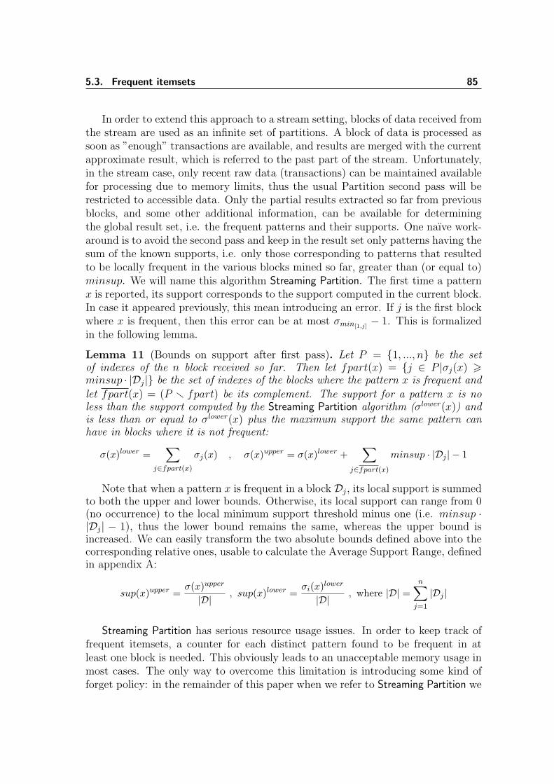
5.3. Frequent itemsets 85
In order to extend this approach to a stream setting, blocks of data received fromthe stream are used as an infinite set of partitions. A block of data is processed assoon as ”enough” transactions are available, and results are merged with the currentapproximate result, which is referred to the past part of the stream. Unfortunately,in the stream case, only recent raw data (transactions) can be maintained availablefor processing due to memory limits, thus the usual Partition second pass will berestricted to accessible data. Only the partial results extracted so far from previousblocks, and some other additional information, can be available for determiningthe global result set, i.e. the frequent patterns and their supports. One naıve work-around is to avoid the second pass and keep in the result set only patterns having thesum of the known supports, i.e. only those corresponding to patterns that resultedto be locally frequent in the various blocks mined so far, greater than (or equal to)minsup. We will name this algorithm Streaming Partition. The first time a patternx is reported, its support corresponds to the support computed in the current block.In case it appeared previously, this mean introducing an error. If j is the first blockwhere x is frequent, then this error can be at most σmin[1,j]
− 1. This is formalizedin the following lemma.
Lemma 11 (Bounds on support after first pass). Let P = {1, ..., n} be the setof indexes of the n block received so far. Then let fpart(x) = {j ∈ P |σj(x) >minsup · |Dj|} be the set of indexes of the blocks where the pattern x is frequent and
let fpart(x) = (P r fpart) be its complement. The support for a pattern x is noless than the support computed by the Streaming Partition algorithm (σlower(x)) andis less than or equal to σlower(x) plus the maximum support the same pattern canhave in blocks where it is not frequent:
σ(x)lower =∑
j∈fpart(x)
σj(x) , σ(x)upper = σ(x)lower +∑
j∈fpart(x)
minsup · |Dj | − 1
Note that when a pattern x is frequent in a block Dj, its local support is summedto both the upper and lower bounds. Otherwise, its local support can range from 0(no occurrence) to the local minimum support threshold minus one (i.e. minsup ·|Dj| − 1), thus the lower bound remains the same, whereas the upper bound isincreased. We can easily transform the two absolute bounds defined above into thecorresponding relative ones, usable to calculate the Average Support Range, definedin appendix A:
sup(x)upper =σ(x)upper
|D|, sup(x)lower =
σi(x)lower
|D|, where |D| =
n∑j=1
|Dj |
Streaming Partition has serious resource usage issues. In order to keep track offrequent itemsets, a counter for each distinct pattern found to be frequent in atleast one block is needed. This obviously leads to an unacceptable memory usage inmost cases. The only way to overcome this limitation is introducing some kind offorget policy: in the remainder of this paper when we refer to Streaming Partition we
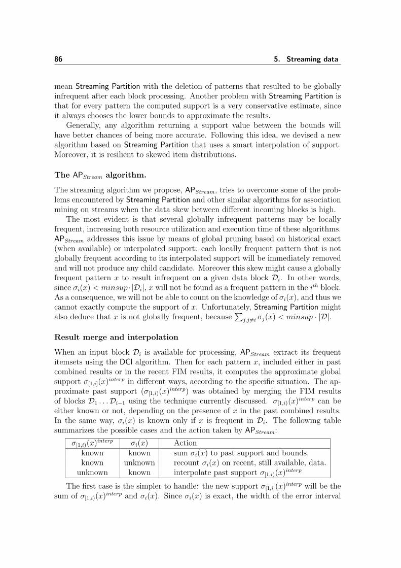
86 5. Streaming data
mean Streaming Partition with the deletion of patterns that resulted to be globallyinfrequent after each block processing. Another problem with Streaming Partition isthat for every pattern the computed support is a very conservative estimate, sinceit always chooses the lower bounds to approximate the results.
Generally, any algorithm returning a support value between the bounds willhave better chances of being more accurate. Following this idea, we devised a newalgorithm based on Streaming Partition that uses a smart interpolation of support.Moreover, it is resilient to skewed item distributions.
The APStream algorithm.
The streaming algorithm we propose, APStream, tries to overcome some of the prob-lems encountered by Streaming Partition and other similar algorithms for associationmining on streams when the data skew between different incoming blocks is high.
The most evident is that several globally infrequent patterns may be locallyfrequent, increasing both resource utilization and execution time of these algorithms.APStream addresses this issue by means of global pruning based on historical exact(when available) or interpolated support: each locally frequent pattern that is notglobally frequent according to its interpolated support will be immediately removedand will not produce any child candidate. Moreover this skew might cause a globallyfrequent pattern x to result infrequent on a given data block Di. In other words,since σi(x) < minsup · |Di|, x will not be found as a frequent pattern in the ith block.As a consequence, we will not be able to count on the knowledge of σi(x), and thus wecannot exactly compute the support of x. Unfortunately, Streaming Partition mightalso deduce that x is not globally frequent, because
∑j,j 6=i σj(x) < minsup · |D|.
Result merge and interpolation
When an input block Di is available for processing, APStream extract its frequentitemsets using the DCI algorithm. Then for each pattern x, included either in pastcombined results or in the recent FIM results, it computes the approximate globalsupport σ[1,i](x)interp in different ways, according to the specific situation. The ap-proximate past support (σ[1,i)(x)interp) was obtained by merging the FIM resultsof blocks D1 . . .Di−1 using the technique currently discussed. σ[1,i)(x)interp can beeither known or not, depending on the presence of x in the past combined results.In the same way, σi(x) is known only if x is frequent in Di. The following tablesummarizes the possible cases and the action taken by APStream:
σ[1,i)(x)interp σi(x) Actionknown known sum σi(x) to past support and bounds.known unknown recount σi(x) on recent, still available, data.
unknown known interpolate past support σ[1,i)(x)interp
The first case is the simpler to handle: the new support σ[1,i](x)interp will be thesum of σ[1,i)(x)interp and σi(x). Since σi(x) is exact, the width of the error interval
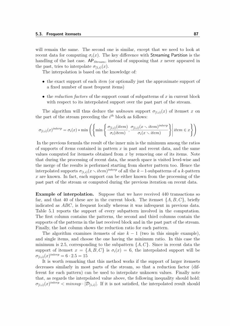
5.3. Frequent itemsets 87
will remain the same. The second one is similar, except that we need to look atrecent data for computing σi(x). The key difference with Streaming Partition is thehandling of the last case. APStream, instead of supposing that x never appeared inthe past, tries to interpolate σ[1,i)(x).
The interpolation is based on the knowledge of:
• the exact support of each item (or optionally just the approximate support ofa fixed number of most frequent items)
• the reduction factors of the support count of subpatterns of x in current blockwith respect to its interpolated support over the past part of the stream.
The algorithm will thus deduce the unknown support σ[1,i)(x) of itemset x onthe part of the stream preceding the ith block as follows:
σ[1,i)(x)interp = σi(x) ∗min
({min
{σ[1,i)(item)σi(item)
,σ[1,i)(x r item)interp
σi(x r item)
}∣∣∣∣∣ item ∈ x
})
In the previous formula the result of the inner min is the minimum among the ratiosof supports of items contained in pattern x in past and recent data, and the samevalues computed for itemsets obtained from x by removing one of its items. Notethat during the processing of recent data, the search space is visited level-wise andthe merge of the results is performed starting from shorter pattern too. Hence theinterpolated supports σ[1,i)(xr item)interp of all the k−1-subpatterns of a k-patternx are known. In fact, each support can be either known from the processing of thepast part of the stream or computed during the previous iteration on recent data.
Example of interpolation. Suppose that we have received 440 transactions sofar, and that 40 of these are in the current block. The itemset {A, B, C}, brieflyindicated as ABC, is frequent locally whereas it was infrequent in previous data.Table 5.1 reports the support of every subpattern involved in the computation.The first column contains the patterns, the second and third columns contain thesupports of the patterns in the last received block and in the past part of the stream.Finally, the last column shows the reduction ratio for each pattern.
The algorithm examines itemsets of size k − 1 (two in this simple example),and single items, and choose the one having the minimum ratio. In this case theminimum is 2.5, corresponding to the subpattern {A, C}. Since in recent data thesupport of itemset x = {A, B, C} is σi(x) = 6, the interpolated support will beσ[1,i)(x)interp = 6 · 2.5 = 15
It is worth remarking that this method works if the support of larger itemsetsdecreases similarly in most parts of the stream, so that a reduction factor (dif-ferent for each pattern) can be used to interpolate unknown values. Finally notethat, as regards the interpolated value above, the following inequality should hold:σ[1,i)(x)interp < minsup · |D[1,i)|. If it is not satisfied, the interpolated result should
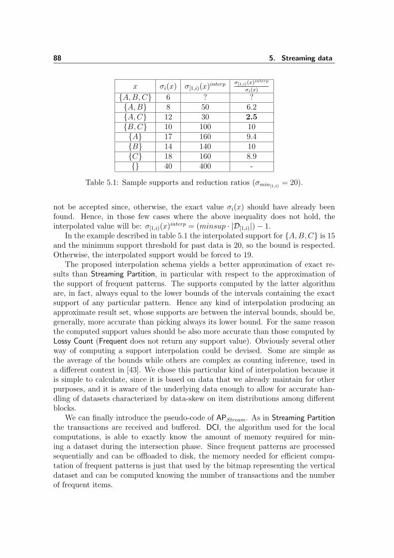
88 5. Streaming data
x σi(x) σ[1,i)(x)interp σ[1,i)(x)interp
σi(x)
{A, B, C} 6 ? ?{A, B} 8 50 6.2{A, C} 12 30 2.5{B, C} 10 100 10{A} 17 160 9.4{B} 14 140 10{C} 18 160 8.9{} 40 400 -
Table 5.1: Sample supports and reduction ratios (σmin[1,t)= 20).
not be accepted since, otherwise, the exact value σi(x) should have already beenfound. Hence, in those few cases where the above inequality does not hold, theinterpolated value will be: σ[1,i)(x)interp = (minsup · |D[1,i)|)− 1.
In the example described in table 5.1 the interpolated support for {A, B, C} is 15and the minimum support threshold for past data is 20, so the bound is respected.Otherwise, the interpolated support would be forced to 19.
The proposed interpolation schema yields a better approximation of exact re-sults than Streaming Partition, in particular with respect to the approximation ofthe support of frequent patterns. The supports computed by the latter algorithmare, in fact, always equal to the lower bounds of the intervals containing the exactsupport of any particular pattern. Hence any kind of interpolation producing anapproximate result set, whose supports are between the interval bounds, should be,generally, more accurate than picking always its lower bound. For the same reasonthe computed support values should be also more accurate than those computed byLossy Count (Frequent does not return any support value). Obviously several otherway of computing a support interpolation could be devised. Some are simple asthe average of the bounds while others are complex as counting inference, used ina different context in [43]. We chose this particular kind of interpolation because itis simple to calculate, since it is based on data that we already maintain for otherpurposes, and it is aware of the underlying data enough to allow for accurate han-dling of datasets characterized by data-skew on item distributions among differentblocks.
We can finally introduce the pseudo-code of APStream. As in Streaming Partitionthe transactions are received and buffered. DCI, the algorithm used for the localcomputations, is able to exactly know the amount of memory required for min-ing a dataset during the intersection phase. Since frequent patterns are processedsequentially and can be offloaded to disk, the memory needed for efficient compu-tation of frequent patterns is just that used by the bitmap representing the verticaldataset and can be computed knowing the number of transactions and the numberof frequent items.
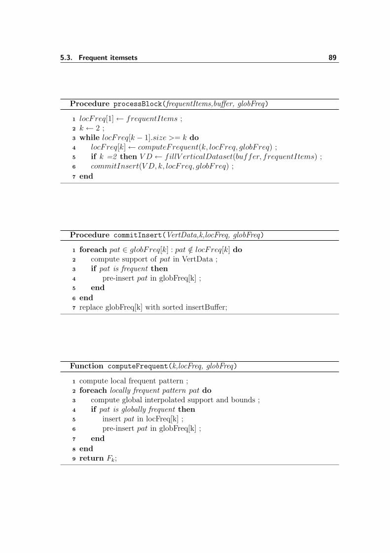
5.3. Frequent itemsets 89
Procedure processBlock(frequentItems,buffer, globFreq)
locFreq[1]← frequentItems ;1
k ← 2 ;2
while locFreq[k − 1].size >= k do3
locFreq[k]← computeFrequent(k, locFreq, globFreq) ;4
if k =2 then V D ← fillV erticalDataset(buffer, frequentItems) ;5
commitInsert(V D, k, locFreq, globFreq) ;6
end7
Procedure commitInsert(VertData,k,locFreq, globFreq)
foreach pat ∈ globFreq[k] : pat /∈ locFreq[k] do1
compute support of pat in VertData ;2
if pat is frequent then3
pre-insert pat in globFreq[k] ;4
end5
end6
replace globFreq[k] with sorted insertBuffer;7
Function computeFrequent(k,locFreq, globFreq)
compute local frequent pattern ;1
foreach locally frequent pattern pat do2
compute global interpolated support and bounds ;3
if pat is globally frequent then4
insert pat in locFreq[k] ;5
pre-insert pat in globFreq[k] ;6
end7
end8
return Fk;9
90 5. Streaming data
Thus, we can use this knowledge in order to maximize the size of the block oftransactions processed at once. For the sake of simplicity we will neglect the quiteobvious main loop with code related to buffering, concentrating on the processingof each data block. The interpolation formula has been omitted too, in the pseudo-code, for the same reason.
Each block is processed, visiting the search space level-wise, for discovering fre-quent patterns. In this way, itemsets are sorted according to their length and theinterpolated support for frequent subpattern is always available when required. Theprocessing of patterns of length k is performed in two steps. First frequent patternsare computed in the current block and then the actual insertion into the currentset of frequent patterns is carried out. When a pattern is found to be frequent inthe current block its support on past data is immediately checked: if it was alreadyknown then the local support is summed to previous support and previous bounds.Otherwise, a support and a pair of bounds are inferred for past data and summedto the support in the current block. In both cases, if the resulting support passthe support test, the pattern is queued for delayed insertion. After every locallyfrequent pattern of the current length k has been processed, the support of everypreviously known pattern that is not locally frequent is computed on recent data.Patterns passing the support test are queued for delayed insertion too. Then theset of pre-inserted itemsets is sorted and the actual insertion take place.
Bounds on computed support errors
As a consequence of using an interpolation method to guess an approximate supportvalue in the past part of the stream, it is very important to establish some boundson the support found for each pattern. In the previous subsection, we have alreadyindicated a pair of really loose bounds: each support cannot be negative, and if apattern was not frequent in a time interval then its interpolated support should beless than the minimum support threshold for the same interval. The lower boundis obviously always satisfied, whereas in case a support value σ[1,i−1](x)interp breaksits upper bound value, it will be forced to (minsup · |D[1,i−1]|) − 1 which is thegreatest value compatible with the bound. This criterion is completely true for non-evolving distributed dataset (distributed frequent pattern mining) or for the firsttwo data block of the stream. In the stream case, the upper bound is based onprevious approximate results, and could be inexact if the pattern corresponds to afalse negative. Nevertheless, it does represent a useful indication.
Bounds based on pattern subset The first bounds that interpolated supportsshould obey, derive from the Apriori property : no set can have a support greaterthan those of any of its subset can. Since recent results are merged level-wise withpreviously known ones, the interpolation can exploit already interpolated subsetsupport. When a subpattern is missing during interpolation this mean that it hasbeen examined during a previous level and discarded. In that case, all of its superset
5.3. Frequent itemsets 91
may be discarded as well. The computed bound is thus affected by the approxima-tion of past results: a pattern with an erroneous support will affect the bounds foreach of its superset. To avoid this issue it is possible to compute the upper boundfor a pattern x simply using the upper bounds of its sub-patterns instead of theirsupport. In this way, the upper bounds will be weaker, but there will be less falsenegatives due to erroneous bounds enforcement.
Bounds based on transaction hash In order to address the issue of error prop-agation in support bounds we need to devise some other kind of bounds that arecomputed exclusively from received data and thus are independent of any previ-ous results. Such bounds can be obtained using inverted transaction hashes. Thistechnique was first introduced in the algorithm IHP [26], an association mining al-gorithm where it was used for finding upper bounds for the support of candidatesin order to prune infrequent ones. As we will show this method can be used alsofor lower bounds. The key idea is that each item has an associated hashed set ofcounters that are accessed by using transaction id as a key. More in detail, eacharray hcnt[item] associated with an item is an array of hsize counters initialized tozero. When the tidth transaction t = {ti} is processed, a hash function transformsthe tid value into an index to be used for the array of counters. Since tids areconsecutive integer numbers, a trivial hash function as h(tid) = tid mod hsize willguarantee an equal repartition of transactions among all hash bins. For each itemti ∈ t the counter at position h(tid) in the array hcnt[ti] is incremented.
The hash function implicitly subdivides the transactions of the dataset. Eachpartition corresponds to a position in the array of counters, while the value ofeach counter represents the number of occurrences of an item in a given set oftransactions. These hashes are a sort of ”compressed” tid-list and can be intersectedto obtain deterministic bounds for the number of occurrences of a specified pattern.Notably these arrays of counters have a fixed size, independent from the number oftransactions processed.
Let hsize = 1, A and B two items and hA = hcnt[A][0] and hB = hcnt[B][0]the only counters contained in their respective hashes, i.e. hA and hB are thenumber of occurrences of items A and B in the whole dataset. According to theApriori principle the support σ({A, B}) for the pattern {A, B} can be at most equalto min(hA, hB). Furthermore, we are able to indicate a lower bound for the samesupport. Let n[i] be the number of transactions associated with the ith hash position,which, in this case, corresponds to the total number of transactions n. We knowfrom the inclusion/exclusion principle that σ({A, B}) should be greater than or atleast equal to max(0,hA + hB − n). In fact if n− hA transactions does not containsthe item A then at least hB− (n−hA) of the hB transactions containing B will alsocontain A. Suppose that n = 10, hA = 8, hB = 7. If we represent with an X eachtransaction supporting a pattern and with a dot any other transaction we obtainthe following diagrams:
92 5. Streaming data
Best case(ub(AB)= 7) Worst case(lb(AB)=5)
A: XXXXXXXX.. XXXXXXXX..
B: XXXXXXX... ...XXXXXXX
AB: XXXXXXX... ...XXXXX..
Then no more than 7 transactions will contain both A and B. At the same timeat least 8 + 7− 10 = 5 transactions will satisfy that constraint. Since each counterrepresents a set of transaction, this operation is equivalent to the computation of theminimal and maximal intersections of the tid-lists associated with the single items.
Usually hsize will be larger than one. In that case, the previously explainedcomputations will be applied to each hash position, yielding an array of lower boundsand an array of upper bounds. The sums of their elements will give the pair ofbounds for pattern {A, B} as we will show in the following example. Let hsize = 3,h(tid) = tid mod hsize the hash function, A and B two items and n[i] = 10 bethe number of transactions associated with the ith hash position. Suppose thathcnt[A] = {8, 4, 6} and hcnt[B] = {7, 5, 6}. Using the same notation previouslyintroduced we obtain:
h(tid)=0 h(tid)=1 h(tid)=2
Best case Worst case Best case Worst case Best case Worst case
A: XXXXXXXX.. XXXXXXXX.. A: XXXX...... XXXX...... A: XXXXXX.... XXXXXX....
B: XXXXXXX... ...XXXXXXX B: XXXXX..... .....XXXXX B: XXXXXX.... ....XXXXXX
AB: XXXXXXX... ...XXXXX.. AB: XXXX...... .......... AB: XXXXXX.... ....XX....
supp 7 5 supp 4 0 supp 6 2
Each pair of columns represents the transactions having a tid mapped into thecorresponding location by the hash function. The lower and upper bounds for thesupport of pattern AB will be respectively 5 + 0 + 2 = 7 and 7 + 4 + 6 = 17.
Both lower bounds and upper bounds computations can be extended to largeritemsets by associativity: the bounds for the first two items are composed with thethird element counters and so on. The sums of the elements of the last pair ofresulting arrays will be the upper and the lower bounds for the given pattern. Thisis possible since the reasoning previously explained still holds if we considers theoccurrences of itemsets instead of those of single items. The lower bound computedin this way will be often equal to zero in sparse dataset. Conversely, on densedatasets this method did proved to be effective in narrowing the two bounds.
Experimental evaluation
In the final part of this section, we study the behavior of the proposed method. Wehave run the APStream algorithm on several datasets using different parameters. Thegoal of these tests is to understand how similarities of the results vary as the streamlength increases, the effectiveness of the hash-based pruning, and, in general, howdataset peculiarities and invocation parameters affect the accuracy of the results.Furthermore, we studied how execution time evolves in time when the stream lengthincreases.
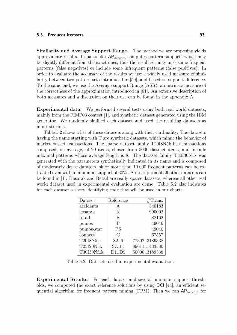
5.3. Frequent itemsets 93
Similarity and Average Support Range. The method we are proposing yieldsapproximate results. In particular APStream computes pattern supports which maybe slightly different from the exact ones, thus the result set may miss some frequentpatterns (false negatives) or include some infrequent patterns (false positives). Inorder to evaluate the accuracy of the results we use a widely used measure of simi-larity between two pattern sets introduced in [50], and based on support difference.To the same end, we use the Average support Range (ASR), an intrinsic measure ofthe correctness of the approximation introduced in [61]. An extensive description ofboth measures and a discussion on their use can be found in the appendix A.
Experimental data. We performed several tests using both real world datasets,mainly from the FIMI’03 contest [1], and synthetic dataset generated using the IBMgenerator. We randomly shuffled each dataset and used the resulting datasets asinput streams.
Table 5.2 shows a list of these datasets along with their cardinality. The datasetshaving the name starting with T are synthetic datasets, which mimic the behavior ofmarket basket transactions. The sparse dataset family T20I8N5k has transactionscomposed, on average, of 20 items, chosen from 5000 distinct items, and includemaximal patterns whose average length is 8. The dataset family T30I30N1k wasgenerated with the parameters synthetically indicated in its name and is composedof moderately dense datasets, since more than 10,000 frequent patterns can be ex-tracted even with a minimum support of 30%. A description of all other datasets canbe found in [1]. Kosarak and Retail are really sparse datasets, whereas all other realworld dataset used in experimental evaluation are dense. Table 5.2 also indicatesfor each dataset a short identifying code that will be used in our charts.
Dataset Reference #Trans.accidents A 340183kosarak K 990002retail R 88162pumbs P 49046pumbs-star PS 49046connect C 67557T20I8N5k S2..6 77302..3189338T25I20N5k S7..11 89611..1433580T30I30Nf1k D1..D9 50000..3189338
Table 5.2: Datasets used in experimental evaluation.
Experimental Results. For each dataset and several minimum support thresh-olds, we computed the exact reference solutions by using DCI [44], an efficient se-quential algorithm for frequent pattern mining (FPM). Then we ran APStream for
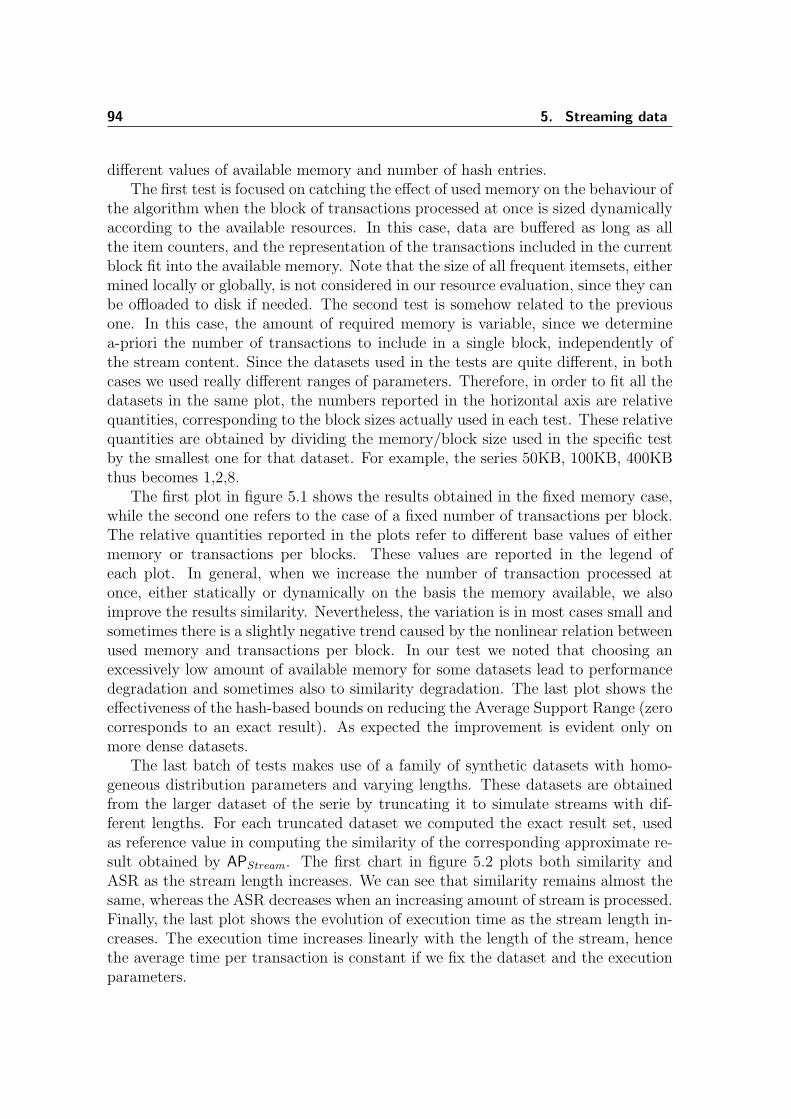
94 5. Streaming data
different values of available memory and number of hash entries.The first test is focused on catching the effect of used memory on the behaviour of
the algorithm when the block of transactions processed at once is sized dynamicallyaccording to the available resources. In this case, data are buffered as long as allthe item counters, and the representation of the transactions included in the currentblock fit into the available memory. Note that the size of all frequent itemsets, eithermined locally or globally, is not considered in our resource evaluation, since they canbe offloaded to disk if needed. The second test is somehow related to the previousone. In this case, the amount of required memory is variable, since we determinea-priori the number of transactions to include in a single block, independently ofthe stream content. Since the datasets used in the tests are quite different, in bothcases we used really different ranges of parameters. Therefore, in order to fit all thedatasets in the same plot, the numbers reported in the horizontal axis are relativequantities, corresponding to the block sizes actually used in each test. These relativequantities are obtained by dividing the memory/block size used in the specific testby the smallest one for that dataset. For example, the series 50KB, 100KB, 400KBthus becomes 1,2,8.
The first plot in figure 5.1 shows the results obtained in the fixed memory case,while the second one refers to the case of a fixed number of transactions per block.The relative quantities reported in the plots refer to different base values of eithermemory or transactions per blocks. These values are reported in the legend ofeach plot. In general, when we increase the number of transaction processed atonce, either statically or dynamically on the basis the memory available, we alsoimprove the results similarity. Nevertheless, the variation is in most cases small andsometimes there is a slightly negative trend caused by the nonlinear relation betweenused memory and transactions per block. In our test we noted that choosing anexcessively low amount of available memory for some datasets lead to performancedegradation and sometimes also to similarity degradation. The last plot shows theeffectiveness of the hash-based bounds on reducing the Average Support Range (zerocorresponds to an exact result). As expected the improvement is evident only onmore dense datasets.
The last batch of tests makes use of a family of synthetic datasets with homo-geneous distribution parameters and varying lengths. These datasets are obtainedfrom the larger dataset of the serie by truncating it to simulate streams with dif-ferent lengths. For each truncated dataset we computed the exact result set, usedas reference value in computing the similarity of the corresponding approximate re-sult obtained by APStream. The first chart in figure 5.2 plots both similarity andASR as the stream length increases. We can see that similarity remains almost thesame, whereas the ASR decreases when an increasing amount of stream is processed.Finally, the last plot shows the evolution of execution time as the stream length in-creases. The execution time increases linearly with the length of the stream, hencethe average time per transaction is constant if we fix the dataset and the executionparameters.
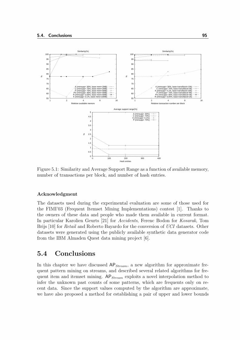
5.4. Conclusions 95
55
60
65
70
75
80
85
90
95
100
1 2 4 8 16
%
Reletive available memory
Similarity(%)
A (minsupp= 30%, base mem=2MB)C (minsupp= 70%, base mem=2MB)P (minsupp= 70%, base mem=5MB)
PS (minsupp= 40%, base mem=5MB)R (minsupp= 0.05%, base mem=5MB)K (minsupp= 0.1%, base mem=16MB)
55
60
65
70
75
80
85
90
95
100
1 2 4 8 16
%
Relative transaction number per block
Similarity(%)
A (minsupp= 30%, base trans/block=10k)C (minsupp= 70%, base trans/block=4k)
K (minsupp= 0.1%, base trans/block=20k)P (minsupp= 70%, base trans/block=8k)
PS (minsupp= 40%, base trans/block=4k)R (minsupp= 0.05%, base trans/block=2k)
0
0.5
1
1.5
2
2.5
3
3.5
4
4.5
5
0 100 200 300 400
%
Hash entries
Average support range(%)
A (minsupp= 30%)C (minsupp= 70%)K (minsupp= 0.1%)P (minsupp= 70%)
Figure 5.1: Similarity and Average Support Range as a function of available memory,number of transactions per block, and number of hash entries.
Acknowledgment
The datasets used during the experimental evaluation are some of those used forthe FIMI’03 (Frequent Itemset Mining Implementations) contest [1]. Thanks tothe owners of these data and people who made them available in current format.In particular Karolien Geurts [21] for Accidents, Ferenc Bodon for Kosarak, TomBrijs [10] for Retail and Roberto Bayardo for the conversion of UCI datasets. Otherdatasets were generated using the publicly available synthetic data generator codefrom the IBM Almaden Quest data mining project [6].
5.4 Conclusions
In this chapter we have discussed APStream, a new algorithm for approximate fre-quent pattern mining on streams, and described several related algorithms for fre-quent item and itemset mining. APStream exploits a novel interpolation method toinfer the unknown past counts of some patterns, which are frequents only on re-cent data. Since the support values computed by the algorithm are approximate,we have also proposed a method for establishing a pair of upper and lower bounds
96 5. Streaming data
99
99.2
99.4
99.6
99.8
100
1 2 4 8 16 32 0
0.05
0.1
0.15
0.2
Sim
ilarit
y (%
)
AS
R (
%)
Stream length (/100k)
dataset: T30I30N1k min_supp=30%
SimilarityASR
1
2
4
8
16
32
1 2 4 8 16 32
Rel
ativ
e tim
e
Stream length (/100k)
dataset: T30I30N1k min_supp=30%
relative time
Figure 5.2: Similarity and Average Support Range as a function of different streamlengths.
for each interpolated value. These bounds are computed using the knowledge ofsubpattern frequency in past data and the intersection of a hash based compressedrepresentation of past data.
Experimental tests show that the solution produced by APStream is a good ap-proximation of the exact global result. The comparisons with exact results considerboth the set of patterns found and their support. The metric used in order to assessthe quality of the algorithm output is the similarity measure introduced in [50].The interpolation works particularly well for dense dataset, achieving a similarityclose to 100% in best cases. The adaptive behaviour of APStream allows us to limitthe amount of used memory. As expected, we have found that a larger amount ofavailable memory corresponds to a more accurate result. Furthermore, as the lengthof the processed stream increases, the similarity with the exact result remains al-most the same. At the same time, we observed a decrease in the average differencebetween upper and lower bounds, which is an intrinsic measure of result accuracy.This means that when the stream length increase, the relative bounds on supportget closer. Finally, the time needed to process a block of transactions does notdepend on the stream length, hence the total execution time is linear with respectto the stream length. In the future, we plan to improve the proposed method byadding other stricter bounds on the approximate support and to extend it to closedpatterns.


Conclusions
The knowledge discovery process and, particularly, its data mining algorithmic part,have been extensively studied in the literature during the last twenty years, and isstill an active discipline. Several problem and analysis methods have been proposed,and the extraction of valuable and hidden knowledge from operational databases is,currently, a strategic issue for most medium and large companies. Most of these or-ganizations are geographically spread by nature, and distributed database systemsare widely diffused due to either logistic, failure resilience, or performance reasons.Banks, telecommunication companies, wireless access provider, are just some of theusers of distributed system for the management of both historical and operationaldata. Furthermore, in several cases, the data are produce and/or modified continu-ously and at a sustained rate. The usage of data mining algorithms in distributedand stream settings may introduce several challenging issues. Problems may be ei-ther technical, related to the network infrastructure and the huge amount of data,political, related to privacy, company interest or ownership of data. The issues tosolve, however, depend on the kind of knowledge we are interested to extract fromdata.
In this thesis, we have analyzed in detail the issues related to the AssociationRules Mining, and more precisely to its most computationally expensive phase, themining of frequent patterns in distributed dataset and data stream, where thesepatterns can be either itemsets (FIM) or sequences (FSM). The core contributionof this work is a general framework for adapting an exact Frequent Pattern Miningalgorithm to a distributed or streaming context. The resulting algorithms are ableto find efficiently an approximation of the exact results with a strong reduction ofcommunication size, in the distributed case, and memory usage, in the stream case.In both cases, the approximate support of each pattern is returned along with aninterval containing the true value.
The proposed methods have been evaluated in a distributed setting and in astream one, using several real world and synthetic datasets. The results of our testshow that this framework gives a fairly accurate approximation of exact results, evenonly exploiting simple and generic interpolation schemas as those used in the tests.In the distributed case, the interpolation based method exhibits linear speedup asthe number of partitions increases. In the stream case, the time that is required toprocess a block is on average constant, hence the total execution time is linear withrespect to the length of the data stream. At the same time, both the similarity tothe exact results and the absolute width of the error interval are almost constant.Thus, the algorithm is suitable for mining infinite amount of data.
One further original contribution presented in this thesis is an algorithm for
100 Conclusions
frequent sequence mining with gap constraints. CCSM is a novel algorithm forthe discovery of frequent sequence patterns with constraints on the maximum gapbetween the occurrences of two part of the sequence (maxGap). The proposed al-gorithm has been compared with cSPADE, a state of the art algorithm, obtainingbetter performance result for significant value of the maxgap constraint. Thanks tothe particular transversal order of the search space exploited by CCSM, the inter-mediate results are highly reused, and the output is ordered. This is particularlyimportant and allows to efficiently integrate the CCSM algorithm in the proposeddistributed/stream framework, as explained in the next section.
Future works
Frequent Sequence Mining on distributed/stream data
The methods presented for frequent itemset extraction can easily be extended tothe other kind of frequent patterns considered in this thesis: the frequent sequences.This only involves minor modifications of the algorithms: replacing the interpola-tion formula with one suitable for sequences, and the FIM algorithm with a FSMalgorithm. The CCSM algorithm is a suitable FSM candidate to be inserted in ourdistributed and stream framework, since it is level-wise and returns ordered set offrequent sequences. This ordering allows for merging on-the-fly the sequence pat-terns as they arrive, and the level-wise behavior makes more information availableto be exploited by the interpolation schema in order to give a better approximation.Furthermore, the on-the-fly merge reduces both memory requirement and computa-tional cost of the merge phase.
As the overall framework remains exactly the same, all the improvements andlimits that we have explained for frequent itemsets are still valid. The only differ-ences are those originated by the intrinsic difference between frequent itemset andfrequent sequences, which make the result of FSM potentially larger and more likelyto be affected by combinatorial explosion.
Frequent Itemset Mining on distributed stream data
The proposed merge/interpolation framework can be extended seamlessly to managedistributed streams in several ways. The most straightforward one is based onthe composition of APInterp, followed by APStream. Each slave is responsible forextracting frequent itemsets from its local streams. The results of each processedblock are sent to the master and merged, first among them using APInterp, and thenwith the past combined results as in APStream. The schema on the left of Figure IIIillustrates this framework. Resnode,i is the FIM result on the ith block of the nodestream, whereas Resi is the result of the merge of all local ith results, and Hist Resi
is the historical global result, i.e., from the beginning to the ith block.
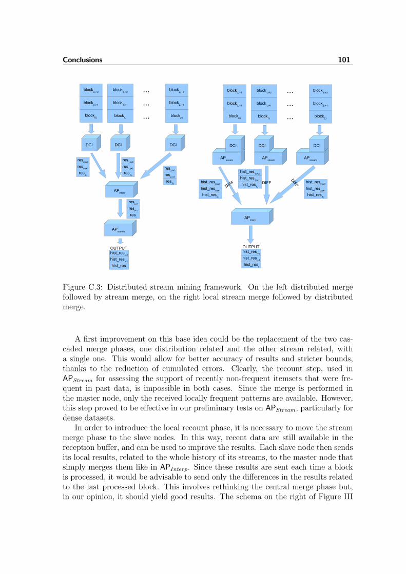
Conclusions 101
Figure C.3: Distributed stream mining framework. On the left distributed mergefollowed by stream merge, on the right local stream merge followed by distributedmerge.
A first improvement on this base idea could be the replacement of the two cas-caded merge phases, one distribution related and the other stream related, witha single one. This would allow for better accuracy of results and stricter bounds,thanks to the reduction of cumulated errors. Clearly, the recount step, used inAPStream for assessing the support of recently non-frequent itemsets that were fre-quent in past data, is impossible in both cases. Since the merge is performed inthe master node, only the received locally frequent patterns are available. However,this step proved to be effective in our preliminary tests on APStream, particularly fordense datasets.
In order to introduce the local recount phase, it is necessary to move the streammerge phase to the slave nodes. In this way, recent data are still available in thereception buffer, and can be used to improve the results. Each slave node then sendsits local results, related to the whole history of its streams, to the master node thatsimply merges them like in APInterp. Since these results are sent each time a blockis processed, it would be advisable to send only the differences in the results relatedto the last processed block. This involves rethinking the central merge phase but,in our opinion, it should yield good results. The schema on the right of Figure III
102 Conclusions
illustrates this framework. DCI result streams are directly processed by APStream,yielding Hist Resnode,i, i.e. the results on the whole node stream at time i. APInterp
collect these results and output the final result Hist Resi.The last aspect to consider is synchronization. Each stream evolves, potentially
at a different rate with respect to other streams. This means that when the streamreception buffer of a node is full other nodes could be still collecting data. Thus, thecollect and merge framework should allow for asynchronous and incremental resultmerge, with some kind of forced periodical synchronization, if needed.
Limiting the combinatorial explosion of the output
It should be noted that, both in the distributed and in the stream settings, the actualtime needed to process a partition is mainly related to the statistical properties ofdata. This problem is not specific to our algorithms. Instead, it is a peculiarity of thefrequent itemset/sequences problems, and is directly linked to the exponential sizeof the result sets. Our goal was to find an approximate solution as close as possibleto the exact one, and this is exactly what we achieved. However, this means that incase the exact solution is huge, the approximate solution will be huge too. In thiscase, if we want to ensure that data can be processed at a given rate, choosing adifferent approach is mandatory.
Two approaches can be devised: the first one is based on alternative represen-tations of results, such as closed/condensed/maximal frequent patterns. As quicklyexplained in the related works of chapter 2, both the result size and the informationon support of patterns decrease from the first to the last of the three problems, butthe presence of a pattern in the results is always certain. The second one, instead,aim at discovering only a useful subset of the result, as in the case of alignmentpatterns [31]. We have done some preliminary work on approximate distributedclosed itemset mining [32], but also the second approach will be matter of furtherinvestigations. We believe it should be particularly effective in the sequence case,which is more affected by the combinatorial explosion problem.
AApproximation assessment
The methods we are proposing yields approximate results. In particular APInterp
computes pattern supports which may be slightly different from the exact ones,thus the result set may miss some frequent pattern (false negatives) or include someinfrequent pattern (false positives). In order to evaluate the accuracy of the resultswe need a measure of similarity between two pattern sets. A widely used one hasbeen introduced in [50], and is based on support difference.
Definition 12 (Similarity). Let A and B respectively be the reference (correct) resultset and the approximate result set. supA(x) ∈ [0, 1] and supB(y) ∈ [0, 1], wherex ∈ A and y ∈ B, correspond to the relative support found in A and B respectively.Note that since B corresponds to the frequent patterns found by the approximatealgorithm under observation, A − B thus corresponds to the set of false negatives,while B − A are the false positives.
The Similarity is thus computed as
Simα(A, B) =
∑x∈A∩B max{0, 1− α ∗ |supA(x)− supB(x)|}
|A ∪ B|
where α > 1 is a scaling parameter, which increase the effect of the support dissim-ilarity. Moreover, 1
αindicates the maximum allowable error on (relative) pattern
supports. We will use the notation Sim() to indicate the default case for α, i.e.α = 1.
In case absolute supports are used instead than relative ones, the parameter αwill be smaller than or equal to 1. We will name this measure Absolute Similarity,indicated as SimABS(A, B).
This measure of similarity is thus the sum of at most |A∩B| values in the range[0, 1], divided by |A ∪B|. Since |A ∩B| 6 |A ∪B|, similarity lies in [0, 1] too.
When a pattern appears in both sets and the difference between the two supportsis greater than 1
α, it does not improve similarity, otherwise similarity is increased
according to the scaled difference. If α = 20, then the maximum allowable error inthe relative support is 1/20 = 0.05 = 5%. Supposing that the support difference fora particular pattern is 4%, the numerator of the similarity measure will be increasedby a small quantity: 1−(20∗0.04) = 0.2. When α is 1 (default value), only patterns
104 A. Approximation assessment
whose support difference is at most 100% contribute to increase similarity. On theother hand, when we set α to a very high value, only patterns with a very similarsupports in both the approximate and reference sets will contribute to increase thesimilarity measure (which is roughly the same than using Absolute Similarity withα close to 1).
It is worth noting that the presence of several false positives and negatives inthe approximate result set B contributes to reduce our similarity measure, since thisentails an increase in A∪B (the denominator of the Simα formula) with respect toA∩B. Moreover, if a pattern has an actual support that is slightly less than minsupbut the approximate support (supB) is slightly greater than minsup, similarityis decreased even if the computed support was almost correct. This could be anundesired behavior. While a false negative can constitute a big issue, because somepotentially important association rules will be not generated at all, a false positivewith a support very close to the exact one could be tolerated by an analyst.
In order to overcome this issue we propose a new similarity measure, fpSim(where fp stand for false positive). Since this measure consider every pattern in-cluded in the approximate result set B (instead of A∩B), it can be used in order toassess whether false positives have an approximate support value close to the exactone or not. A high value of fpSim compared with a smaller value of Sim simplymeans that in the approximate result set B there are several false positive with atrue support close to minsup.
Definition 13 (fpSimilarity). Let A and B respectively be the reference (correct)result set and the approximate result set. supB(x) ∈ [0, 1], where x ∈ B, correspondsto the support found in result sets B, while sup(x) ∈ [0, 1] is the actual support ofthe same pattern. fpSimilarity is thus computed as
fpSimα(A, B) =
∑x∈B max{0, 1− α ∗ |sup(x)− supB(x)|}
|A ∪ B|
where α > 1 is a scaling parameter. We will use the notation Sim() to indicate thedefault case for α, i.e. α = 1.
Note that the numerator of this new measure considers all the patterns foundin the set B, thus also false positives. Hence finding a pattern with a support closeto the true one is considered a ”good” result in any case, even if this pattern isnot actually frequent. For example, suppose that minimum support threshold is50% and x is an infrequent pattern such that sup(x) = 49.9. If supB(x) = 50%, itwill result to be a false positive. However, since supB(x) is very close to the exactsupport sup(x), the value of fpSimα() will be increased.
In Definition 13 we used sup(x) instead of supA(x) to indicate the actual supportof itemset x since it is possible, as in the example case, that a pattern is present inB even if it is not frequent (hence not present in A).
In both definitions above, we used sup(x) to indicate the (relative) support,ranging from 0 to 1. In the remainder of the paper, in particular in the algorithm
105
description, we will also use the notation σ(x) = sup(x) · |D| to indicate the supportcount (absolute support), ranging from 0 to the total number of transactions.
When bounds on the support of each pattern are available, an intrinsic measureof the correctness of the approximation is the average width of the interval betweenthe upper bound and the lower bound.
Definition 14 (Average support range). Let B be the approximate result set, sup(x)the exact support for pattern x and sup(x)lower and sup(x)upper the lower and upperbounds on sup(x), respectively. The average support range is thus defined as:
ASR(B) =1
|B|∑x∈B
sup(x)upper − sup(x)lower
Note that, while this definition can be used for every approximate algorithm, howto compute sup(x)lower and sup(x)upper is algorithm specific. In the next section, wewill present a way that is suitable for the class of algorithms containing the one weare proposing.
Other, less accurate, similarity measures can be borrowed from the InformationRetrieval theory:
Definition 15 (Recall & Precision). Let A and B respectively be the reference (cor-rect) result set and the approximate result set. Note that since B corresponds to thefrequent patterns found by the approximate algorithm under observation, A−B thuscorresponds to the set of false negatives, while B − A are the false positives.
Let P (A, B) ∈ [0, 1] be the Precision of the approximate result, defined as follows:
P (A, B) =B ∩ A
B
Hence the Precision is maximal (P (A, B) = 1) iff B ∩ A = B, i.e. the approximateresult set B is completely contained in the exact one A, and no false positives occurs.
Let R(A, B) ∈ [0, 1] be the Recall of the approximate result, defined as follows:
R(A, B) =B ∩ A
A
Hence the Recall is maximal (R(A, B) = 1) iff B ∩ A = A, i.e. the exact result setA is completely contained in the approximate one B, and no false negative occurs.
According to our remarks above concerning the benefits of the fpSim measure(Def. 13), we have that a ”good” approximate result should be characterized by to avery high Recall, where the supports of the possible false positive patterns should behowever very close to the exact ones. Conversely, in order to minimize the standardmeasure of similarity (Def. 12), we need to maximize both Recall and Precision,while keeping small the difference in the approximate supports of frequent patterns.

106 A. Approximation assessment
Bibliography
[1] Workshop on frequent itemset mining implementations FIMI’03 in conjunctionwith ICDM’03. In fimi.cs.helsinki.fi, 2003.
[2] R. Agarwal, C. Aggarwal, and V. V. V. Prasad. A tree projection algorithmfor generation of frequent itemsets. Parallel and Distributed Computing, 2000.
[3] R. Agarwal, C. Aggarwal, and V.V.V. Prasad. Depth first generation of longpatterns. In KDD ’00: Proceedings of the sixth ACM SIGKDD internationalconference on Knowledge discovery and data mining, pages 108–118, New York,NY, USA, 2000. ACM Press.
[4] R. Agrawal, T. Imielinski, and A. Swami. Mining association rules betweensets of items in large databases. In Proceedings of the 1993 ACM SIGMODInternational Conference on Management of Data, pages 207–216, Washington,D.C., 1993.
[5] R. Agrawal and J.C. Shafer. Parallel mining of association rules. In IEEETransaction On Knowledge and Data Engineering, 1996.
[6] R. Agrawal and R. Srikant. Fast algorithms for mining association rules. InProc. 20th Int. Conf. Very Large Data Bases, VLDB, pages 487–499. MorganKaufmann, 1994.
[7] R. Agrawal and R. Srikant. Mining sequential patterns. In Proc. 11th Int. Conf.Data Engineering, ICDE, pages 3–14. IEEE Press, 1995.
[8] J. Ayres, J. Gehrke, T. Yiu, and J. Flannick. Sequential pattern mining usingbitmaps. In Proceedings of the Eighth ACM SIGKDD International Conferenceon Knowledge Discovery and Data Mining, 2002.
[9] R. J. Bayardo Jr. Efficiently Mining Long Patterns from Databases. In Proc. ofthe ACM SIGMOD Int. Conf. on Management of Data, pages 85–93, Seattle,Washington, USA, 1998.
[10] T. Brijs, G. Swinnen, K. Vanhoof, and G. Wets. Using association rules forproduct assortment decisions: A case study. In Knowledge Discovery and DataMining, pages 254–260, 1999.
[11] D. Burdick, M. Calimlim, and J. Gehrke. Mafia: a maximal frequent itemsetfor transactional databases. In Proc. of the International Conference on DataEndineering ICDE, pages 443–452. IEEE Computer Society, 2001.
108 Bibliography
[12] M. Charikar, K. Chen, and M. Farach-Colton. Finding frequent items in datastreams. In ICALP ’02: Proceedings of the 29th International Colloquium onAutomata, Languages and Programming, pages 693–703, London, UK, 2002.Springer-Verlag.
[13] D.W. Cheung, J. Han, V.T. Ng, A.W. Fu, and Y. Fu. A fast distributedalgorithm for mining association rules. In DIS ’96: Proceedings of the fourthinternational conference on on Parallel and distributed information systems,pages 31–43, Washington, DC, USA, 1996. IEEE Computer Society.
[14] G. Cormode and S. Muthukrishnan. What’s hot and what’s not: trackingmost frequent items dynamically. In PODS ’03: Proceedings of the twenty-second ACM SIGMOD-SIGACT-SIGART symposium on Principles of databasesystems, pages 296–306. ACM Press, 2003.
[15] G. Cormode and S. Muthukrishnan. An improved data stream summary: thecount-min sketch and its applications. J. Algorithms, 55(1):58–75, 2005.
[16] E.D. Demaine, A. Lopez-Ortiz, and J.I. Munro. Frequency estimation of in-ternet packet streams with limited space. In ESA ’02: Proceedings of the 10thAnnual European Symposium on Algorithms, pages 348–360, London, UK, 2002.Springer-Verlag.
[17] C. Estan and G. Varghese. New directions in traffic measurement and account-ing: Focusing on the elephants, ignoring the mice. ACM Trans. Comput. Syst.,21(3):270–313, 2003.
[18] U. M. Fayyad, G. Piatetsky-Shapiro, P. Smyth, and R. Uthurusamy, editors.Advances in Knowledge Discovery and Data Mining. AAAI Press, 1998.
[19] V. Ganti, J. Gehrke, and R. Ramakrishnan. Mining Very Large Databases.IEEE Computer, 32(8):38–45, 1999.
[20] M.N. Garofalakis, R. Rastogi, and K. Shim. SPIRIT: Sequential pattern miningwith regular expression constraints. In The VLDB Journal, pages 223–234,1999.
[21] K. Geurts, G. Wets, T. Brijs, and K. Vanhoof. Profiling high frequency ac-cident locations using association rules. In Proceedings of the 82nd AnnualTransportation Research Board, Washington DC. (USA), January 12-16, page18pp, 2003.
[22] E-H.S. Han, G. Karypis, and V. Kumar. Scalable parallel data mining forassociation rules. In IEEE Transaction on Knowledge and Data Engineering,2000.
Bibliography 109
[23] J. Han and M. Kamber. Data Mining: Concepts and Techniques. MorganKaufmann Publishers, 1st edition, 2000.
[24] J. Han, J. Pei, B. Mortazavi-Asi, Q. Chen, U. Dayal, and M.-C. Hsu. Freespan:Frequent pattern-projected sequential pattern mining. In In Proc. ACM 6thInt. Conf. on Knowledge Discovery and Data Mining, pages 355–359, 2000.
[25] J. Han, J. Pei, and Y. Yin. Mining frequent patterns without candidate gener-ation. In Proc. of the ACM SIGMOD Int. Conference on Management of Data,2000.
[26] J.D. Holt and S.M. Chung. Mining association rules using inverted hashing andpruning. Inf. Process. Lett., 83(4):211–220, 2002.
[27] V.C. Jensen and N. Soparkar. Frequent itemset counting across multiple tables.In In 4th PAcific Asia Conference on Knowledge Discovery and Data Minig,2000.
[28] C. Jin, W. Qian, C. Sha, J.X. Yu, and A. Zhou. Dynamically maintainingfrequent items over a data stream. In CIKM ’03: Proceedings of the twelfth in-ternational conference on Information and knowledge management, pages 287–294, New York, NY, USA, 2003. ACM Press.
[29] R. Jin and G. G. Agrawal. An algorithm for in-core frequent itemset miningon streaming data. To appear in ICDM’05, 2005.
[30] R.M. Karp, S. Shenker, and C.H. Papadimitriou. A simple algorithm for findingfrequent elements in streams and bags. ACM Transactions on Database Systems(TODS), 28(1):51–55, 2003.
[31] H. Kum, J. Pei, W. Wang, and D. Duncan. ApproxMAP: Approximate miningof consensus sequential patterns. In Proceedings of the Third InternationalSIAM Conference on Data Mining, 2003.
[32] C. Lucchese, S. Orlando, R. Perego, and C. Silvestri. Mining frequent closeditemsets from highly distributed repositories. In Proc. of the 1st CoreGRIDWorkshop on Knowledge and Data Management in Grids in conjunction withPPAM2005, September 2005.
[33] G. Manku and R. Motwani. Approximate frequency counts over data streams.In In Proceedings of the 28th International Conference on Very Large DataBases, August 2002.
[34] H. Mannila and H. Toivonen. Discovering generalized episodes using minimaloccurrences. In Knowledge Discovery and Data Mining, pages 146–151, 1996.
110 Bibliography
[35] H. Mannila, H. Toivonen, and A. I. Verkamo. Discovering Frequent Episodes inSequences. In Proceedings of the First International Conference on KnowledgeDiscovery and Data Mining (KDD-95), Montreal, Canada, 1995. AAAI Press.
[36] H. Mannila, H. Toivonen, and A.I. Verkamo. Discovery of frequent episodes inevent sequences. Data Mining and Knowledge Discovery, 1(3):259–289, 1997.
[37] F. Masseglia, F. Cathala, and P. Poncelet. The PSP approach for miningsequential patterns. In Principles of Data Mining and Knowledge Discovery,pages 176–184, 1998.
[38] F. Masseglia, P. Poncelet, and M. Teisseire. Incremental mining of sequentialpatterns in large databases. Technical report, LIRMM, France, January 2000.
[39] F. Masseglia, P. Poncelet, and M. Teisseire. Incremental mining of sequentialpatterns in large databases. Data and Knowledge Engineering, 46(1):97–121,2003.
[40] J. Misra and D. Gries. Finding repeated elements. Technical report, Ithaca,NY, USA, 1982.
[41] A. Mueller. Fast sequential and parallel algorithms for association rules mining:A comparison. Technical Report CS-TR-3515, Univ. of Maryland, 1995.
[42] S. Orlando, P. Palmerini, and R. Perego. Enhancing the apriori algorithm forfrequent set counting. In DaWaK ’01: Proceedings of the Third InternationalConference on Data Warehousing and Knowledge Discovery, pages 71–82, Lon-don, UK, 2001. Springer-Verlag.
[43] S. Orlando, P. Palmerini, R. Perego, C. Lucchese, and F. Silvestri. kDCI: amulti-strategy algorithm for mining frequent sets. In Proceedings of the work-shop on Frequent Itemset Mining Implementations FIMI’03 in conjunction withICDM’03, 2003.
[44] S. Orlando, P. Palmerini, R. Perego, and F. Silvestri. Adaptive and resource-aware mining of frequent sets. In Proc. of the 2002 IEEE International Con-ference on Data Mining, ICDM, 2002.
[45] S. Orlando, P. Palmerini, R. Perego, and F. Silvestri. An efficient paralleland distributed algorithm for counting frequent sets. In Proc. of Int. Conf.VECPAR 2002 - LNCS 2565, pages 197–204. Spinger, 2002.
[46] S. Orlando, R. Perego, and C. Silvestri. CCSM: an efficient algorithm forconstrained sequence mining. In Proceedings of the 6th International Workshopon High Performance Data Mining: Pervasive and Data Stream Mining, inconjunction with Third International SIAM Conference on Data Mining, 2003.
Bibliography 111
[47] S. Orlando, R. Perego, and C. Silvestri. A new algorithm for gap constrainedsequence mining. To appear in Proceedings of ACM Symposim on AppliedComputing SAC - Data Mining track, Nicosia, Cyprus, March 2004.
[48] B. Park and H. Kargupta. Distributed Data Mining: Algorithms, Systems, andApplications. In Data Mining Handbook, pages 341–358. IEA, 2002.
[49] J.S. Park, M.S. Chen, and P.S. Yu. An Effective Hash Based Algorithm forMining Association Rules. In Proceedings of 1995 ACM SIGMOD Int. Conf.on Management of Data, pages 175–186.
[50] S. Parthasarathy. Efficient progressive sampling for association rules. InProceedings of the 2002 IEEE International Conference on Data Mining(ICDM’02), page 354. IEEE Computer Society, 2002.
[51] S. Parthasarathy, M.J. Zaki, M. Ogihara, and S. Dwarkadas. Incremental andinteractive sequence mining. In CIKM, pages 251–258, 1999.
[52] J. Pei, J. Han, B. Mortazavi-Asl, H. Pinto, Q. Chen, U. Dayal, and M.-C. Hsu.Prefixspan: Mining sequential patterns efficiently by prefix-projected patterngrowth. In Proceedings of the 17th International Conference on Data Engineer-ing, page 215. IEEE Computer Society, 2001.
[53] J. Pei, J. Han, and W. Wang. Mining sequential patterns with constraints inlarge databases. In Proc. of Proceedings of the 11-th Int. Conf. on Informationand Knowledge Management (CIKM 02), pages 18–25, 2002.
[54] N. Ramakrishnan and A. Y. Grama. Data Mining: From Serendipity to Science.IEEE Computer, 32(8):34–37, 1999.
[55] A. Savasere, E. Omiecinski, and S.B. Navathe. An efficient algorithm for miningassociation rules in large databases. In VLDB’95, Proceedings of 21th Inter-national Conference on Very Large Data Bases, pages 432–444. Morgan Kauf-mann, September 1995.
[56] A. Schuster and R. Wolff. Communication Efficient Distributed Mining of As-sociation Rules. In ACM SIGMOD, Santa Barbara, CA, April 2001.
[57] A. Schuster, R. Wolff, and D. Trock. A High-Performance Distributed Algo-rithm for Mining Association Rules. In The Third IEEE International Confer-ence on Data Mining (ICDM’03), Melbourne, FL, November 2003.
[58] T. Shintani and M. Kitsuregawa. Hash based parallel algorithms for miningassociation rules. In PDIS: International Conference on Parallel and DistributedInformation Systems. IEEE Computer Society Technical Committee on DataEngineering, and ACM SIGMOD, 1996.
112 Bibliography
[59] C. Silvestri and S. Orlando. Distributed association mining: an approximatemethod. In Proceedings of 7th International Workshop on High Performanceand Distributed Mining, in conjunction with Fourth International S, April 2004.
[60] C. Silvestri and S. Orlando. Approximate mining of frequent patterns onstreams. In Proc. of the 2nd International Workshop on Knowledge Discov-ery from Data Streams in conjunction with PKDD2005, October 2005.
[61] C. Silvestri and S. Orlando. Distributed approximate mining of frequent pat-terns. In Proceedings of ACM Symposim on Applied Computing SAC - DataMining track, March 2005.
[62] R. Srikant and R. Agrawal. Mining sequential patterns: Generalizations andperformance improvements. In Proc. 5th Int. Conf. Extending Database Tech-nology, EDBT, volume 1057, pages 3–17. Springer-Verlag, 1996.
[63] R. Wolff and A. Schuster. Mining Association Rules in Peer-to-Peer Systems.In The Third IEEE International Conference on Data Mining (ICDM’03), Mel-bourne, FL, November 2003.
[64] X. Yan, J. Han, and R. Afshar. Clospan: Mining closed sequential patterns inlarge datasets. In Proc. 2003 SIAM Int.Conf. on Data Mining (SDM’03), 2003.
[65] M.J. Zaki. Fast mining of sequential patterns in very large databases. TechnicalReport TR668, University of Rochester, Computer Science Department, 1997.
[66] M.J. Zaki. Parallel and distributed association mining: A survey. In IEEEConcurrency, 1999.
[67] M.J. Zaki. Parallel sequence mining on shared-memory machines. In Large-Scale Parallel Data Mining, pages 161–189, 1999.
[68] M.J. Zaki. Scalable algorithms for association mining. IEEE Transactions onKnowledge and Data Engineering, 12:372–390, May/June 2000.
[69] M.J. Zaki. Sequence mining in categorical domains: incorporating constraints.In Proceedings of the ninth international conference on Information and knowl-edge management, pages 422–429. ACM Press, 2000.
[70] M.J. Zaki. Spade: An efficient algorithm for mining frequent sequences. Ma-chine Learning, 42(1-2):31–60, 2001.
List of PhD Thesis
TD-2004-1 Moreno Marzolla”Simulation-Based Performance Modeling of UML Software Architectures”
TD-2004-2 Paolo Palmerini”On performance of data mining: from algorithms to management systems fordata exploration”
TD-2005-1 Chiara Braghin”Static Analysis of Security Properties in Mobile Ambients”
TD-2006-1 Fabrizio Furano”Large scale data access: architectures and performance”
TD-2006-2 Damiano Macedonio”Logics for Distributed Resources”
TD-2006-3 Matteo Maffei”Dynamic Typing for Security Protocols”
TD-2006-4 Claudio Silvestri”Distributed and Stream Data Mining Algorithms for Frequent Pattern Dis-covery”