discussion paper no. 8562 - econstor.eu
TRANSCRIPT
econstorMake Your Publications Visible.
A Service of
zbwLeibniz-InformationszentrumWirtschaftLeibniz Information Centrefor Economics
Farber, Henry
Working Paper
Why You Can't Find a Taxi in the Rain and OtherLabor Supply Lessons from Cab Drivers
IZA Discussion Papers, No. 8562
Provided in Cooperation with:IZA – Institute of Labor Economics
Suggested Citation: Farber, Henry (2014) : Why You Can't Find a Taxi in the Rain and OtherLabor Supply Lessons from Cab Drivers, IZA Discussion Papers, No. 8562, Institute for theStudy of Labor (IZA), Bonn
This Version is available at:http://hdl.handle.net/10419/104672
Standard-Nutzungsbedingungen:
Die Dokumente auf EconStor dürfen zu eigenen wissenschaftlichenZwecken und zum Privatgebrauch gespeichert und kopiert werden.
Sie dürfen die Dokumente nicht für öffentliche oder kommerzielleZwecke vervielfältigen, öffentlich ausstellen, öffentlich zugänglichmachen, vertreiben oder anderweitig nutzen.
Sofern die Verfasser die Dokumente unter Open-Content-Lizenzen(insbesondere CC-Lizenzen) zur Verfügung gestellt haben sollten,gelten abweichend von diesen Nutzungsbedingungen die in der dortgenannten Lizenz gewährten Nutzungsrechte.
Terms of use:
Documents in EconStor may be saved and copied for yourpersonal and scholarly purposes.
You are not to copy documents for public or commercialpurposes, to exhibit the documents publicly, to make thempublicly available on the internet, or to distribute or otherwiseuse the documents in public.
If the documents have been made available under an OpenContent Licence (especially Creative Commons Licences), youmay exercise further usage rights as specified in the indicatedlicence.
www.econstor.eu
DI
SC
US
SI
ON
P
AP
ER
S
ER
IE
S
Forschungsinstitut zur Zukunft der ArbeitInstitute for the Study of Labor
Why You Can’t Find a Taxi in the Rain andOther Labor Supply Lessons from Cab Drivers
IZA DP No. 8562
October 2014
Henry S. Farber
Why You Can’t Find a Taxi in the Rain
and Other Labor Supply Lessons from Cab Drivers
Henry S. Farber Princeton University
and IZA
Discussion Paper No. 8562 October 2014
IZA
P.O. Box 7240 53072 Bonn
Germany
Phone: +49-228-3894-0 Fax: +49-228-3894-180
E-mail: [email protected]
Any opinions expressed here are those of the author(s) and not those of IZA. Research published in this series may include views on policy, but the institute itself takes no institutional policy positions. The IZA research network is committed to the IZA Guiding Principles of Research Integrity. The Institute for the Study of Labor (IZA) in Bonn is a local and virtual international research center and a place of communication between science, politics and business. IZA is an independent nonprofit organization supported by Deutsche Post Foundation. The center is associated with the University of Bonn and offers a stimulating research environment through its international network, workshops and conferences, data service, project support, research visits and doctoral program. IZA engages in (i) original and internationally competitive research in all fields of labor economics, (ii) development of policy concepts, and (iii) dissemination of research results and concepts to the interested public. IZA Discussion Papers often represent preliminary work and are circulated to encourage discussion. Citation of such a paper should account for its provisional character. A revised version may be available directly from the author.
IZA Discussion Paper No. 8562 October 2014
ABSTRACT
Why You Can’t Find a Taxi in the Rain and Other Labor Supply Lessons from Cab Drivers*
In a seminal paper, Camerer, Babcock, Loewenstein, and Thaler (1997) find that the wage elasticity of daily hours of work New York City (NYC) taxi drivers is negative and conclude that their labor supply behavior is consistent with target earning (having reference dependent preferences). I replicate and extend the CBLT analysis using data from all trips taken in all taxi cabs in NYC for the five years from 2009-2013. Using the model of expectations-based reference points of Koszegi and Rabin (2006), I distinguish between anticipated and unanticipated daily wage variation and present evidence that only a small fraction of wage variation (about 1/8) is unanticipated so that reference dependence (which is relevant only in response to unanticipated variation) can, at best, play a limited role in determining labor supply. The overall pattern in my data is clear: drivers tend to respond positively to unanticipated as well as anticipated increases in earnings opportunities. This is consistent with the neoclassical optimizing model of labor supply and does not support the reference dependent preferences model. I explore heterogeneity across drivers in their labor supply elasticities and consider whether new drivers differ from more experienced drivers in their behavior. I find substantial heterogeneity across drivers in their elasticities, but the estimated elasticities are generally positive and only rarely substantially negative. I also find that new drivers with smaller elasticities are more likely to exit the industry while drivers who remain learn quickly to be better optimizers (have positive labor supply elasticities that grow with experience). JEL Classification: J22, D01, D03 Keywords: labor supply, reference dependent preferences Corresponding author: Henry S. Farber Industrial Relations Section Firestone Library Princeton University Princeton, NJ 08544 USA E-mail: [email protected]
* This paper is based on my Albert Rees Lecture at the annual meeting of the Society of Labor Economists, May 2, 2014, Arlington, VA. The author thanks participants in workshops at the Federal Reserve Bank of Atlanta, Princeton University, MIT, and Harvard University for their helpful comments.
1 Introduction
That it is difficult to find a taxi in the rain has been a standard complaint in Manhattan
for as long as there have been taxis. If asked why this is the case, the answer from an
economist 20 years ago would have been that rainy weather increases the demand for taxi
rides and there is no or an insufficiently rapid supply response to meet this transitory demand
increase. That answer may have changed in the last 15 years. In their seminal work, Camerer,
Babcock, Loewenstein, and Thaler (1997), referred to here as CBLT, present evidence, based
on a regression of log daily hours on log average hourly earnings, suggesting that the daily
labor supply function of taxi drivers is negatively sloped so that a transitory change in the
wage results in a reduction in hours worked. On this basis, they characterize taxi drivers
as having reference-dependent preferences, which can be summarized simply by saying that
workers will set a daily income target and generally work until that target is met. Others
have also found that labor supply curves for taxi drivers appear to slope downward, and
the consensus of much of this work is that taxi drivers are, in fact, target earners.1 This
suggests an alternative answer to the question of why it is difficult to find a taxi in the rain:
To the extent that drivers have a daily income target and a rain-induced increase in demand
increases earnings, drivers will reach their targets sooner and quit driving for the day. The
new view then is that at least part of the reason you can’t find a taxi in the rain is because
drivers reach their daily earnings targets quickly and go home so that the demand increase
is exacerbated by the resulting decline in supply.2
The question of whether reference dependence plays a substantial role in labor supply
decisions is important, both intellectually and in designing public tax and transfer policies.
In this study, I replicate and extend the CBLT analysis using new data on taxi drivers to
revisit the question of whether the daily labor supply function of taxi drivers slopes down-
ward and whether it is reasonable to characterize taxi drivers as having reference dependent
preferences. My analysis is based on the complete records of all taxi drivers in New York City
over the 5-year period from 2009-2013. This addresses a weakness of much of the earlier work
on taxi drivers, including my own, that the analyses are based on very small convenience
1 See, for example, Chou (2002) and Agarwal, Diao, Pan, and Sing (2013) for estimates of labor supplymodels for taxi drivers that find a negative slope. Using different approaches, Crawford and Meng (2011) andDoran (2014) also find support for reference-dependent preferences in analyses of labor supply of NYC taxidrivers. Koszegi and Rabin (2006) and Ordonez, Schweitzer, Galinsky, and Bazerman (2009) are examplesof how this result has been accepted generally.
2 See Camerer (1997) and Ordonez, Schweitzer, Galinsky, and Bazerman (2009) for explicit statementsthat reference-dependent preferences are an explanation for difficulty in finding a taxi in the rain.
1
samples.
There is a natural tension between the standard neoclassical optimizing model of labor
supply and the model based on reference dependent preferences. Setting income targets is an
inefficient way to earn money because it implies working less on high wage days and working
more on low wage days. The neoclassical model implies the opposite. Clearly, over a period
of days, the neoclassical optimizer works fewer hours than the target earner to earn the same
income.3 Given the efficiency advantage of optimizing behavior, after investigating the slope
of the labor supply function I investigate whether drivers differ in their labor supply behavior
(are some drivers target earners while others are optimizers?). I then investigate whether
new drivers learn to be better optimizers and whether drivers who not strong optimizers
disproportionately quit the industry.
A continuing focus of this “battle of models” is the daily hours decisions of taxi drivers,
and, with some exceptions, the model used is a regression of log daily hours on the log
daily wage (the log of daily average hourly earnings). This is why I focus on estimating the
slope of the daily hours function here, but this modeling approach is not fully appropriate
given that the hourly wage is variable over the day and is uncertain ex ante. In my earlier
work (Farber, 2005, 2008), I took a different empirical approach by modeling the stopping
decision of a driver, where the driver decides at the completion of each trip whether to
continue driving or to end the shift.4 Using this approach, I found that taxi driver labor
supply is best characterized by the neoclassical model and that there is little evidence in
support of reference-dependent preferences.5 I leave for future work analysis of the stopping
model of taxi driver labor supply using the new data.
3 This is the point of the taxi driver example used by Ordonez, Schweitzer, Galinsky, and Bazerman(2009).
4 This stopping decision may be a function of many things, including accumulated hours, accumulatedincome, time of day, day of week, location in the city, etc.
5 Crawford and Meng (2011), using the same data on NYC taxi drivers, extend my earlier work with astopping model that allows for reference points in both daily income and daily hours, and they conclude thatthe data are consistent with this dual reference point model. The empirical evidence from other settingsusing a variety of methods is mixed. Oettinger (1999) examines the labor supply of stadium vendors atbaseball games and finds evidence that labor supply on the extensive margin (number vendors showing upfor games) is consistent with the neoclassical model. Fehr and Goette (2007) run a field experiment varyingthe piece rate paid to bicycle messengers. Their evidence is generally consistent with the neoclassical modelin that messengers work more in months with high piece rates. On the other hand, they interpret evidencethat messengers work fewer hours per day on days in months with high piece rates as evidence of reference-dependent preferences. See also Nguyen and Leung (2009) for an analysis labor supply in fisheries that findsevidence consistent with reference-dependent preferences. Camerer (2000) presents a nice survey of evidencefrom the field on loss aversion and reference dependence in a variety of settings.
2
I turn now to my replication and extension, based on the new data, of the earlier work
estimating the slope of the labor supply function. The next section outlines the competing
theories of labor supply, where I rely heavily on the work of Koszegi and Rabin (2006), who
provide a clear theoretical analysis of the determination of reference points and a guide to
the kind of wage variation that drives reference dependence. In section 3, I present some
background information on the taxi industry in New York City and a broad description of
the data. Section 4 contains my analysis of the why taxis are hard to find in the rain. In
section 5, I describe the construction of the analysis sample and present estimates of the
labor supply function, and, in section 6, I investigate how the slope of the labor supply
function is related to the deviation of the daily wage from its expected value. Section 7
contains an analysis of the extent to which the elasticity of labor supply and the implied
underlying model differs across drivers. In section 8, I investigate whether drivers learn to be
better optimizers (develop larger labor supply elasticities), and, in section 9, I ask whether
drivers who appear to be weaker optimizers (have smaller labor supply elasticities) at the
start of their time as a driver are more likely to exit the industry. Section 10 contains final
remarks and conclusions.
2 Setting the Stage: Competing Theories of Labor
Supply
In the standard neoclassical inter-temporal model of labor supply, individuals work in period
t until the shadow value of time (a function of lifetime wealth/income and increasing in
hours in a given period) equals the period t wage rate.6 The model implies that there is
intertemporal substitution in labor supply across periods so that a transitory increase in the
wage rate in period t implies an increase in period t labor supply because the shadow value
of time conditional on hours is unaffected. However, a permanent change in the wage will
have an offsetting income effect as lifetime wealth increases, increasing the shadow value of
time conditional on hours.7
The reference dependent model of choice has its roots in the literature on loss-aversion
6 See MaCurdy (1981) for an early empirical analysis of inter-temporal substitution in labor supply.Blundell and MaCurdy (1999) present a relatively recent survey of the literature on labor supply.
7 See Ashenfelter, Doran, and Schaller (2010) for an analysis of the effect of two fare increases (1996 and2004) on the labor supply of NYC taxi drivers. They find an elasticity of -0.2 in response to these permanentfare increases.
3
(Tversky and Kahneman (1991). In the context of the daily labor supply decisions of taxi
drivers, the basic idea of the reference dependent preference model is that a driver has in mind
a particular reference level of daily income, and utility as a function of income is evaluated
relative to this reference level. The loss in utility from failing to reach the reference income
level by some amount exceeds the gain in utility from exceeding the reference income level
by the same amount. In other words, the individual is loss averse. There is a kink in the
utility function at the reference income level, with higher marginal utility below the kink
and lower marginal utility above the kink.
Consider the following simple model of labor supply with reference-dependent preferences.
Individuals facing a wage rate W receive utility from income (Y = Wh) and disutility from
hours of work (h). Individuals have a kink in their utility function at some reference level of
income (T ):
U(Y, h) = (1 + α)(Y − T )− θ
1 + νh1+ν Y < T (1)
U(Y, h) = (1− α)(Y − T )− θ
1 + νh1+ν Y ≥ T (2)
where the parameter α > 0 controls the change in marginal utility at the reference point,
θ indexes the disutility of hours, and ν is a parameter related to the elasticity of labor
supply. This specification follows the model of Koszegi and Rabin (2006), where utility
with reference dependent preferences is additive in the usual “consumption utility” and in
a “gain-loss” utility around the reference point. The terms introduced by the parameter α
(±α(Y − T )) represent the gain-loss utility. The rest is the consumption utility (a function
of income and hours).
Maximizing this utility function with respect to hours of work yields three distinct labor
supply functions depending on the wage.8
• For sufficiently low wages (W < W ∗), the reference point is not relevant because the
hours required to reach the reference point at such a low wage yield sufficient disutility
of hours that it is optimal to stop on the high marginal utility section of the utility
function (short of the reference point). In this region, the labor supply function is
h =
((1 + α)W
θ
)1/ν
(3)
8 Note that the neoclassical model is the special case where there is no kink (α = 0). The labor supplyfunction in this case is h = (Wθ )1/ν , and the elasticity of labor supply is 1
ν .
4
with elasticity of labor supply 1/ν > 0.
• For intermediate wage levels (W ∗ < W < W ∗∗), it is optimal to stop working upon
reaching the reference income level. This is because the wage is in a range that is high
enough to reward working when marginal utility is high (Y < T ) but too low to reward
working when marginal utility is low (Y ≥ T ). In this region, the individual is a target
earner with labor supply function
h =T
W(4)
and elasticity of labor supply is -1.
• For sufficiently high wages (W > W ∗∗), the reference point is not relevant because the
wage is sufficiently high that it is optimal to operate on the low marginal utility section
of the utility function (beyond the reference point). In this region, the labor supply
function is
h =
((1− α)W
θ
)1/ν
(5)
with elasticity of labor supply 1/ν > 0.
The bounds of the range where reference-dependent preferences are relevant are derived
from the optimizing behaviour of the individuals. Consider first the lower bound, W ∗. The
value of W ∗ is defined as the wage at which an individual with the “steep” utility function
defined in equation 1 would choose hours so as to earn T . Based on the labor supply function
in equation 3, this is
W ∗ =
(θ
1 + α
) 11+ν
Tν
1+ν . (6)
Consider next the upper bound, W ∗∗. The value of W ∗∗ is defined as the wage at which an
individual with the “flat” utility function defined in equation 2 would choose hours so as to
earn T . Based on the labor supply function in equation 5, this is
W ∗∗ =
(θ
1− α
) 11+ν
Tν
1+ν . (7)
The ratio of the upper bound to the lower bound is
W ∗∗
W ∗ =
(1 + α
1− α
)( 11+ν
)
, (8)
and this is directly related the degree of gain-loss utility (indexed by α) and the labor supply
elasticity (measured inversely by ν). If α is close to zero, indicating little gain-loss utility, the
5
range of wages where the individual is a target earner is very small, and reference dependence
is not important. But as α grows, reference dependence and target earnings behavior have
more relevance.
Koszegi and Rabin (2006) suggest that the reference income level will be based on ex-
pected income.9 Expected income will be driven by the income level generated by the ex-
pected wage and the hours choice made by the individual based on the expected wage. Defin-
ing reference points in this way, as reflecting expected income, has important implications,
both for thinking about the potential importance of reference dependence in determining
labor supply and in designing an empirical analysis that reflects appropriate variation.
The Koszegi-Rabin model of expectation-based reference income levels suggests impor-
tantly that labor supply will be positively related to anticipated transitory wage changes.
They argue that reference dependence (gain-loss utility in their terms) is related only to
unanticipated variation in the wage. In periods where high wages are expected, individu-
als will have higher reference points implying higher labor supply as the neoclassical model
predicts. The prediction of the reference dependent preferences model, that the elasticity
of labor supply is -1, is relevant only with regard to unanticipated transitory wage changes
that are close to the expected wage. This limits how much of labor supply behavior can be
accounted for by reference dependent preferences and suggests that much of the variability
in labor supply is likely to be consistent with the neoclassical model.10 Later, I decom-
pose variation in average hourly earnings into components that are plausibly interpreted as
permanent, anticipated transitory, and unanticipated transitory.
I now use the Koszegi-Rabin formulation of expectation-based reference points to derive
the bounds (W ∗ and W ∗∗ in equations 6 and 7 respectively) as a function of the expected
wage. In order to simplify the exposition given the multiplicative functional forms, I work
with the logarithm of the wage and hours and the expectation of the logarithms. The
expected log labor supply based on the consumption part of the utility function is
E(`n(h)) =1
νE(`n(W ))− 1
νθ, (9)
9 Abeler, Falk, Goette, and Huffman (2011) present experimental evidence that variation in work effort isconsistent with reference points based on expectations. Crawford and Meng (2011) rely on expectation-basedreference points in their analysis of taxi driver labor supply.
10 Doran (2014) reaches a similar conclusion based on his analysis of a relatively small sample of shifts.Crawford and Meng (2011), building on the Koszegi-Rabin work, also recognize that the response to antici-pated transitory wage changes will be neoclassical.
6

and the log income reference point is
`n(T ) = E(`n(h)) + E(`n(W ))
=1 + ν
νE(`n(W ))− 1
νθ. (10)
The bounds are related to the expected wage through the reference income level. Sub-
stituting the expression in equation 10 for the log reference income level into the logarithms
of equations 6 and 7 yields particularly simple expressions for the logarithms of the bounds
(W ∗ and W ∗∗). These are
`n(W ∗) = E(`n(W ))−(
1
1 + ν
)`n(1 + α), (11)
and
`n(W ∗∗) = E(`n(W ))−(
1
1 + ν
)`n(1− α). (12)
The likelihood that the realized wage is outside the bounds, yielding neoclassical behavior
(positive labor supply elasticity) is a function of how variable the wage is around its expected
value. If the wage has only small unanticipated variation (since anticipated variation is built
into the reference income level through the expected wage), then behavior in response to
unanticipated transitory wage variation will generally look like target earning. On the other
hand, if the wage has substantial unanticipated variation, then behavior will be neoclassical.
This formulation of the labor supply model with reference dependent preferences has a
direct empirical prediction: On days when the wage rate unexpectedly varies substantially
from its expected value, labor supply will be more likely to vary directly with the wage rate.
But on days where the wage rate is relatively close to expectation, hours worked will be
more likely to vary inversely with the relatively small unanticipated wage variation.
3 Background and Data on Taxi Drivers
There are 13,238 taxi medallions in New York City. This number is set by regulation.
Roughly speaking, there are two types of medallions.
1. Fleet medallions, of which there 7,664, are attached (literally) to taxis generally oper-
ated through a fleet garage and leased on a daily shift basis to individual drivers with
hack licenses.11 Owners of fleet medallions must own at least two medallions, and each
11 Less commonly, taxis with fleet medallions are leased on a weekly basis.
7
fleet medallion must operate for two shifts of at least 9 hours per day. It is not clear
if or how the latter requirement is enforced.
2. Independent medallions, of which there are 5,574, are owned by individuals who may
own no more than one medallion. A subset of these medallions are “owner-driver”
medallions, which have a requirement that a substantial number of shifts in taxis with
such medallions be driven by the owner. Other independent medallions have no such
restriction, and these taxis may or may not be driven by the owner. In either case,
taxis with independent medallions may be leased for shifts to drivers with hack licenses
who are not the owner. Again, it is not clear if or how these requirements are enforced.
The standard employment arrangement of New York City cab drivers who do not own
their own cabs/medallions is that a driver leases a cab for a fixed period, usually a 12-hour
shift. The driver pays a fixed fee for the cab plus fuel, and he keeps 100 percent of the
fare income plus tips. The driver is free to work as few or as many hours as he wishes
within a 12-hour shift. Thus, the driver internalizes the costs and benefits of working in a
way that is largely consistent with an economist’s first-best solution to the agency problem
with risk-neutral agents. In a manner of speaking, the employer has “sold the firm to the
worker.” Because these drivers are free to set their hours once they have leased a taxi for a
shift, analysis of their labor supply is fertile ground for learning about behavioral models.
Taxi drivers earn income only when there is a passenger in the cab. My data cover the
2009-2013 period. Prior to September 4, 2012, income was earned was earned at the rate of
$2.50 for the first one-fifth mile (the “meter drop” ) plus $.40 per additional one-fifth of a
mile when travelling at 12 miles per hour or more plus $.40 for each minute when travelling
at less than 12 miles per hour (waiting time). From September 4, 2012 through 2013, the rate
for additional fifths of a mile and waiting minutes was increased from $.40 income to $.50.
Throughout the period, there was also a night surcharge of $.50 per trip between 8PM and
6AM and peak-hour weekday surcharge of $1.00 Monday-Friday between 4PM and 8PM.12
Clearly, a central factor in earnings is the ease/speed with which new fares are located.
The earlier studies of taxi driver labor supply were based on analysis of relatively small
numbers of hand-written “trip sheets”(one per shift) that drivers were required to fill out
with information on the fare and trip start and end times and locations. These sheets were
12 There is a flat fare of $52.00 ($45.00 prior to September 4, 2012) plus tolls between Manhattan andJFK International Airport in either direction and a surcharge of $17.50 ($15.00 prior to September 4, 2012)on trips to Newark Liberty International Airport.
8
difficult to read accurately, and the limited number of sheets available severely constrained
analysis.
This situation has changed dramatically. The New York City Taxi and Limousine Com-
mission (TLC), the agency charged with regulating the industry, now requires all taxis to
be equipped with electronic devices that record all trip information including fares, times,
and locations. The (currently two) companies that supply these devices report all this in-
formation to the TLC on a regular basis, and I have obtained full information for all trips
taken in NYC taxi cabs for the five years from 2009-2013. These data, called TPEP by the
TLC, identify drivers by encrypted hack license number and medallions (cabs) by encrypted
medallion number.
There are approximately 180 million trips taken during approximately 8 million shifts
each year in taxi cabs in NYC. About 62,000 drivers had at least one fare in a cab over the
five-year period, with about 40,000 drivers in any single year. About 25,000 drivers worked
in all five years. In fact, these are more data than I can use efficiently, and much of my
analysis is based on a random sub-sample of 2/15 of the drivers.
An important limitation of the data is that I cannot identify fleet and independent medal-
lions, let alone isolate the owner-driver medallions among the independent medallions.13 It
may be that owner-drivers face different incentives regarding labor supply than do drivers
who lease their cabs, whether from a fleet owner or an individual. For this reason, it would
be useful to analyze their labor supply separately. However, I am forced to use all drivers,
regardless of medallion type.
Another limitation of the data is that complete information is not available on tip receipts.
Data on tips are available only for fares with tips paid by credit card. While the percentage
of fares paid by credit card has been increasing over time, about 46 percent of fares in the
most recent year (2013) were paid in cash and so there is no tip information. Tips on credit
card transactions averaged about 20 percent over the 2009-2013 period. I proceed ignoring
tips due to the missing data for cash transactions, and this will not cause a problem for my
analysis unless variation the rate of tipping is correlated with hourly fare income.14
13 The TLC knows which medallions are fleet medallions and which are independent medallions. However,they have not made this information available in a way that can be used with the detailed data on driveractivity. The TLC does not have complete information on which of the independent medallions are owner-driver medallions.
14 See Haggag and Paci (2014) for an analysis of tipping behavior in NYC taxi cabs in 2009.
9
4 Why Can’t You Find a Taxi in the Rain?
I begin with a direct analysis of the question of whether or not target earnings behavior
can account for some of the perceived difficulty in finding a cab in the rain. The underlying
idea is that when it is raining taxi drivers earn more per unit time and so reach their daily
earnings targets sooner and quit for the day.
Rain may have a number of effects on the market for taxi rides. First, it likely increases
demand. This will make it easier for drivers to find passengers and increase hourly income.
However, rain may decrease speed due to congestion and a deterioration in general driving
conditions, which could result in lower earnings. Rain may also make driving less pleasant,
implying a reduction in the number of cabs on the road having nothing to do with target
earnings behavior.
For this analysis, I use a random sub-sample of the drivers in the data described above.
These data include all trips taken by 2/15 of the drivers I see between 2009 and 2013. This
sub-sample includes 116,177,329 trips for 8,802 drivers.
In order to examine the market, I use the trip-level data to calculate the average of
income, time with a passenger in the cab, miles travelled, and number of taxis on the street
for each of the 48,824 clock hours in the 5 year period from 2009-2013. I then merge these
data with data on hourly rainfall in Central Park.15 I calculate the hourly wage for a given
driver in a given hour using the trip-level fare and time information. The hourly wage was
computed by dividing each shift into minutes and assigning a “minute wage” to each minute.
For minutes during trips, the minute wage is computed as the fare divided by the number of
minutes for that trip. For minutes of waiting time (between fares), the minute wage is set
to zero. The hourly wage for each clock hour is computed as the sum of the minute wages
during that hour. I calculate time with a passenger in the cab and miles travelled during a
given clock hour in an analogous fashion. The count of taxis on the street is a count of taxis
who had a passenger in the cab for at least one minute during the clock hour.
A necessary condition for target earnings behavior to contribute to difficulty in finding
a taxi in the rain is that hourly earnings be higher when it is raining. The first row of table
1 contains the coefficient of an hourly indicator for precipitation in Central Park from OLS
regression analyses of average log hourly earnings.16 The estimates in column (A) include no
15 Source: National Weather Service (NWS) of the National Oceanic and Atmospheric Administration(NOA) and the Network for Environment and Weather Applications, Cornell University.
16 The indicator for precipitation equals one if there is any precipitation in Central Park recorded during
10
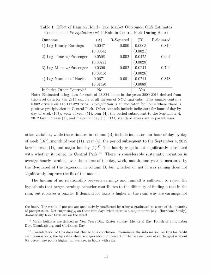
Table 1: Effect of Rain on Hourly Taxi Market Outcomes, OLS Estimates
Coefficient of Precipitation (=1 if Rain in Central Park During Hour)
Outcome (A) R-Squared (B) R-Squared
1) Log Hourly Earnings -0.0047 0.000 -0.0003 0.879
(0.0054) (0.0021)
2) Log Time w/Passenger 0.0508 0.002 0.0475 0.904
(0.0077) (0.0028)
3) Log Miles w/Passenger -0.0306 0.002 -0.0241 0.792
(0.0046) (0.0026)
4) Log Number of Hacks -0.0671 0.001 -0.0711 0.878
(0.0149) (0.0089)
Includes Other Controls? No YesNote: Estimated using data for each of 43,824 hours in the years 2009-2013 derived fromtrip-level data for the 2/15 sample of all drivers of NYC taxi cabs. This sample contains8,802 drivers on 116,117,329 trips. Precipitation is an indicator for hours where there ispositive precipitation in Central Park. Other controls include indicators for hour of day byday of week (167), week of year (51), year (4), the period subsequent to the September 4,2012 fare increase (1), and major holiday (1). HAC standard errors are in parentheses.
other variables, while the estimates in column (B) include indicators for hour of day by day
of week (167), month of year (11), year (4), the period subsequent to the September 4, 2012
fare increase (1), and major holiday (1).17 The hourly wage is not significantly correlated
with whether it rained in Central Park.18 There is considerable systematic variation in
average hourly earnings over the course of the day, week, month, and year as measured by
the R-squared of the regression in column B, but whether or not it was raining does not
significantly improve the fit of the model.
The finding of no relationship between earnings and rainfall is sufficient to reject the
hypothesis that target earnings behavior contributes to the difficulty of finding a taxi in the
rain, but it leaves a puzzle: If demand for taxis is higher in the rain, why are earnings not
the hour. The results I present are qualitatively unaffected by using a graduated measure of the quantityof precipitation. Not surprisingly, on those rare days when there is a major storm (e.g., Hurricane Sandy),dramatically fewer taxis are on the street.
17 Major holidays are defined as New Years Day, Easter Sunday, Memorial Day, Fourth of July, LaborDay, Thanksgiving, and Christmas Day.
18 Consideration of tips does not change this conclusion. Examining the information on tips for creditcard transactions, the tip rate (which averages about 20 percent of the fare inclusive of surcharges) is about0.2 percentage points higher, on average, in hours with rain.
11
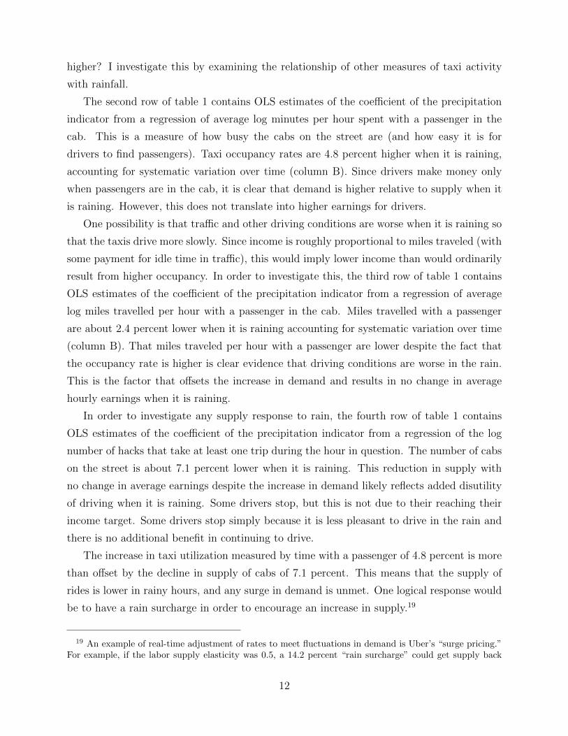
higher? I investigate this by examining the relationship of other measures of taxi activity
with rainfall.
The second row of table 1 contains OLS estimates of the coefficient of the precipitation
indicator from a regression of average log minutes per hour spent with a passenger in the
cab. This is a measure of how busy the cabs on the street are (and how easy it is for
drivers to find passengers). Taxi occupancy rates are 4.8 percent higher when it is raining,
accounting for systematic variation over time (column B). Since drivers make money only
when passengers are in the cab, it is clear that demand is higher relative to supply when it
is raining. However, this does not translate into higher earnings for drivers.
One possibility is that traffic and other driving conditions are worse when it is raining so
that the taxis drive more slowly. Since income is roughly proportional to miles traveled (with
some payment for idle time in traffic), this would imply lower income than would ordinarily
result from higher occupancy. In order to investigate this, the third row of table 1 contains
OLS estimates of the coefficient of the precipitation indicator from a regression of average
log miles travelled per hour with a passenger in the cab. Miles travelled with a passenger
are about 2.4 percent lower when it is raining accounting for systematic variation over time
(column B). That miles traveled per hour with a passenger are lower despite the fact that
the occupancy rate is higher is clear evidence that driving conditions are worse in the rain.
This is the factor that offsets the increase in demand and results in no change in average
hourly earnings when it is raining.
In order to investigate any supply response to rain, the fourth row of table 1 contains
OLS estimates of the coefficient of the precipitation indicator from a regression of the log
number of hacks that take at least one trip during the hour in question. The number of cabs
on the street is about 7.1 percent lower when it is raining. This reduction in supply with
no change in average earnings despite the increase in demand likely reflects added disutility
of driving when it is raining. Some drivers stop, but this is not due to their reaching their
income target. Some drivers stop simply because it is less pleasant to drive in the rain and
there is no additional benefit in continuing to drive.
The increase in taxi utilization measured by time with a passenger of 4.8 percent is more
than offset by the decline in supply of cabs of 7.1 percent. This means that the supply of
rides is lower in rainy hours, and any surge in demand is unmet. One logical response would
be to have a rain surcharge in order to encourage an increase in supply.19
19 An example of real-time adjustment of rates to meet fluctuations in demand is Uber’s “surge pricing.”For example, if the labor supply elasticity was 0.5, a 14.2 percent “rain surcharge” could get supply back
12
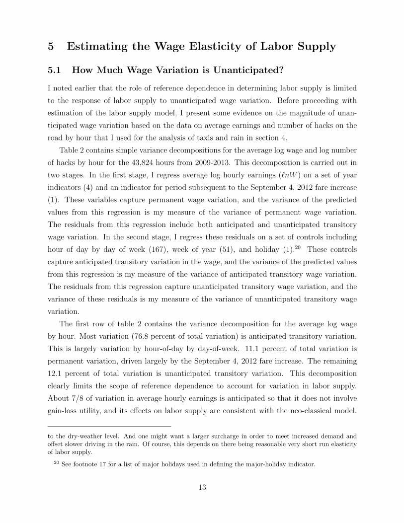
5 Estimating the Wage Elasticity of Labor Supply
5.1 How Much Wage Variation is Unanticipated?
I noted earlier that the role of reference dependence in determining labor supply is limited
to the response of labor supply to unanticipated wage variation. Before proceeding with
estimation of the labor supply model, I present some evidence on the magnitude of unan-
ticipated wage variation based on the data on average earnings and number of hacks on the
road by hour that I used for the analysis of taxis and rain in section 4.
Table 2 contains simple variance decompositions for the average log wage and log number
of hacks by hour for the 43,824 hours from 2009-2013. This decomposition is carried out in
two stages. In the first stage, I regress average log hourly earnings (`nW ) on a set of year
indicators (4) and an indicator for period subsequent to the September 4, 2012 fare increase
(1). These variables capture permanent wage variation, and the variance of the predicted
values from this regression is my measure of the variance of permanent wage variation.
The residuals from this regression include both anticipated and unanticipated transitory
wage variation. In the second stage, I regress these residuals on a set of controls including
hour of day by day of week (167), week of year (51), and holiday (1).20 These controls
capture anticipated transitory variation in the wage, and the variance of the predicted values
from this regression is my measure of the variance of anticipated transitory wage variation.
The residuals from this regression capture unanticipated transitory wage variation, and the
variance of these residuals is my measure of the variance of unanticipated transitory wage
variation.
The first row of table 2 contains the variance decomposition for the average log wage
by hour. Most variation (76.8 percent of total variation) is anticipated transitory variation.
This is largely variation by hour-of-day by day-of-week. 11.1 percent of total variation is
permanent variation, driven largely by the September 4, 2012 fare increase. The remaining
12.1 percent of total variation is unanticipated transitory variation. This decomposition
clearly limits the scope of reference dependence to account for variation in labor supply.
About 7/8 of variation in average hourly earnings is anticipated so that it does not involve
gain-loss utility, and its effects on labor supply are consistent with the neo-classical model.
to the dry-weather level. And one might want a larger surcharge in order to meet increased demand andoffset slower driving in the rain. Of course, this depends on there being reasonable very short run elasticityof labor supply.
20 See footnote 17 for a list of major holidays used in defining the major-holiday indicator.
13
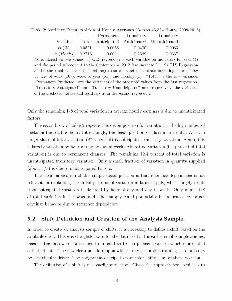
Table 2: Variance Decomposition of Hourly Averages (Across 43,824 Hours, 2009-2013)
Permanent Transitory Transitory
Variable Total Anticipated Anticipated Unanticipated
`n(W ) 0.0521 0.0058 0.0400 0.0063
`n(Hacks) 0.2716 0.0011 0.2369 0.0337Note: Based on two stages: 1) OLS regression of each variable on indicators for year (4)
and the period subsequent to the September 4, 2012 fare increase (1). 2) OLS Regression
of the the residuals from the first regression on a set of controls including hour of day
by day of week (167), week of year (51), and holiday (1). “Total” is the raw variance.
“Permanent Predicted” are the variances of the predicted values from the first regression.
“Transitory Anticipated” and “Transitory Unanticipated” are, respectively, the variances
of the predicted values and residuals from the second regression.
Only the remaining 1/8 of total variation in average hourly earnings is due to unanticipated
factors.
The second row of table 2 repeats this decomposition for variation in the log number of
hacks on the road by hour. Interestingly, the decomposition yields similar results. An even
larger share of total variation (87.2 percent) is anticipated transitory variation. Again, this
is largely variation by hour-of-day by day-of-week. Almost no variation (0.4 percent of total
variation) is due to permanent changes. The remaining 12.4 percent of total variation is
unanticipated transitory variation. Only a small fraction of variation in quantity supplied
(about 1/8) is due to unanticipated factors.
The clear implication of this simple decomposition is that reference dependence is not
relevant for explaining the broad patterns of variation in labor supply, which largely result
from anticipated variation in demand by hour of day and day of week. Only about 1/8
of total variation in the wage and labor supply could potentially be influenced by target
earnings behavior due to reference dependence.
5.2 Shift Definition and Creation of the Analysis Sample
In order to create an analysis sample of shifts, it is necessary to define a shift based on the
available data. This was straightforward for the data used in the earlier small-sample studies,
because the data were transcribed from hand-written trip sheets, each of which represented
a distinct shift. The new electronic data upon which I rely is simply a running list of all trips
by a particular driver. The assignment of trips to particular shifts is an analytic decision.
The definition of a shift is necessarily subjective. Given the approach here, which is to
14
model the shift-level labor supply decision of a driver (perhaps with some reference income
level for the shift), it makes sense to define a shift as composed of all trips that are part
of a sequence that the driver considers to be a single shift. Absent a clear guide, I define
any gap between trips of more than six hours (more than 360 minutes) as marking the end
of one shift and the beginning of the next. Defining shifts in this way yields a sample of
5,047,343 shifts for 8,802 drivers over the period from the 2/15 random sample of all drivers
from 2009-2013. I now present some data that support this choice as a reasonable way to
identify shifts.
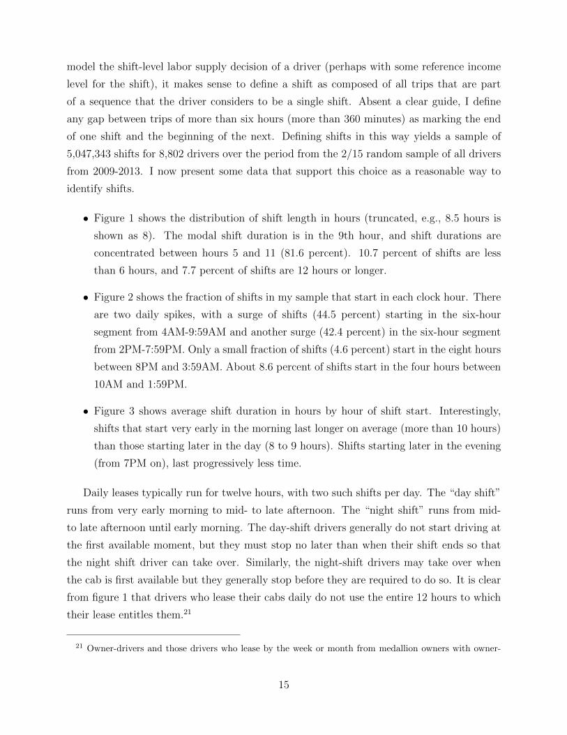
• Figure 1 shows the distribution of shift length in hours (truncated, e.g., 8.5 hours is
shown as 8). The modal shift duration is in the 9th hour, and shift durations are
concentrated between hours 5 and 11 (81.6 percent). 10.7 percent of shifts are less
than 6 hours, and 7.7 percent of shifts are 12 hours or longer.
• Figure 2 shows the fraction of shifts in my sample that start in each clock hour. There
are two daily spikes, with a surge of shifts (44.5 percent) starting in the six-hour
segment from 4AM-9:59AM and another surge (42.4 percent) in the six-hour segment
from 2PM-7:59PM. Only a small fraction of shifts (4.6 percent) start in the eight hours
between 8PM and 3:59AM. About 8.6 percent of shifts start in the four hours between
10AM and 1:59PM.
• Figure 3 shows average shift duration in hours by hour of shift start. Interestingly,
shifts that start very early in the morning last longer on average (more than 10 hours)
than those starting later in the day (8 to 9 hours). Shifts starting later in the evening
(from 7PM on), last progressively less time.
Daily leases typically run for twelve hours, with two such shifts per day. The “day shift”
runs from very early morning to mid- to late afternoon. The “night shift” runs from mid-
to late afternoon until early morning. The day-shift drivers generally do not start driving at
the first available moment, but they must stop no later than when their shift ends so that
the night shift driver can take over. Similarly, the night-shift drivers may take over when
the cab is first available but they generally stop before they are required to do so. It is clear
from figure 1 that drivers who lease their cabs daily do not use the entire 12 hours to which
their lease entitles them.21
21 Owner-drivers and those drivers who lease by the week or month from medallion owners with owner-
15
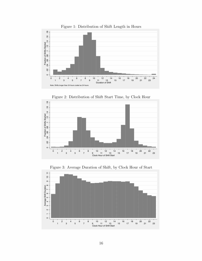
Figure 1: Distribution of Shift Length in Hours
0.0
2.0
4.0
6.0
8.1
.12
.14
.16
.18
Frac
tion
of S
hifts
Sta
rted
01
23
45
67
89
1011
1213
1415
1617
1819
2021
2223
24
Duration of ShiftNote: Shifts longer than 24 hours coded as 24 hours
Figure 2: Distribution of Shift Start Time, by Clock Hour
0.0
2.0
4.0
6.0
8.1
.12
.14
.16
.18
Frac
tion
of S
hifts
Sta
rted
01
23
45
67
89
1011
1213
1415
1617
1819
2021
2223
Clock Hour of Shift Start
Figure 3: Average Duration of Shift, by Clock Hour of Start
01
23
45
67
89
1011
Aver
age
Shift
Dur
atio
n
01
23
45
67
89
1011
1213
1415
1617
1819
2021
2223
Clock Hour of Shift Start
16
I assign shifts as “day” or “night” based on the information in figures 1-3. I define shifts
that start between 4AM and 9:59AM as day shifts (44.5 percent of shifts). I define shifts
that start between 2PM and 7:59PM as night shifts (42.4 percent of shifts). The remaining
13.1 percent of shifts, starting between 10AM and 1:59PM or between 8PM and 3:59AM,
are unclassified (not classified by me as day or night). Drivers who start in late morning or
early afternoon may be day shift drivers who are getting a late start or night shift drivers
who are getting an early start.
There may be an important difference in the margin on which labor supply can be
adjusted on day shifts versus night shifts. Day shift drivers are more likely to be constrained
at the end of their shift when the cab must be turned over to a night shift driver. This implies
that day shift drivers may adjust hours by changing their start time and is consistent with
the decrease in average shift duration, shown in figure 3, as the early morning progresses
from 4AM through 10AM. In contrast, night shift drivers may not be able to start early but
can adjust hours by changing their end time. As demand declines late at night, many of
these drivers stop. The decline in demand late is reflected in the declining average duration
of shifts apparent in figure 3 as starting time moves later in the evening (after 6PM). These
patterns are a natural consequence of the 2-shift structure of the day.
The difference in the active margin of decision making between day and night shifts is
important for analyzing labor supply. Day shift drivers often select hours before information
on unanticipated daily earnings opportunities is revealed. In contrast, night shift drivers can
experience the evolution of earnings opportunities and decide when to quit for the day. If
labor supply is affected by unanticipated transitory variation in earnings opportunities and
if information about these earnings opportunities are learned by the driver only after he has
started the shift, then night shift drivers will have more opportunity than day shift drivers
to adjust their labor supply in response. Operationally, this suggests that estimated labor
supply elasticities could be larger for night shift drivers.
Table 3 contains mean hours, income, and average hourly earnings by shift type.22 Day
shifts are longer than night shifts by about 0.7 hours, but more money is earned on night shifts
(about $13 more). Average hourly earnings (the wage) is about $3.73 higher on the night
shift. All differences in means across shifts are statistically significant (p-value < 10−100).
driver medallions may not be constrained to 12 hour shifts. Their constraints depend on whether there is asecond driver who leases (or sub-leases) the cab. Drivers who lease taxis with fleet medallions daily are soconstrained.
22 Income is defined as the sum of fare income and surcharges. Tip income is not included.
17
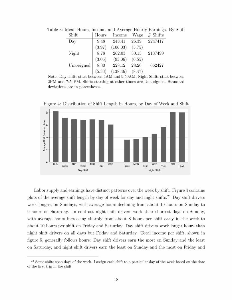
Table 3: Mean Hours, Income, and Average Hourly Earnings. By ShiftShift Hours Income Wage # Shifts
Day 9.48 248.41 26.39 2247417
(3.97) (106.03) (5.75)
Night 8.78 262.03 30.13 2137499
(3.05) (93.06) (6.55)
Unassigned 8.30 228.12 28.26 662427
(5.33) (138.46) (8.47)Note: Day shifts start between 4AM and 9:59AM. Night Shifts start between2PM and 7:59PM. Shifts starting at other times are Unassigned. Standarddeviations are in parentheses.
Figure 4: Distribution of Shift Length in Hours, by Day of Week and Shift
67
89
10Av
erag
e Sh
ift D
urat
ion,
Hou
rs
Day Shift Night Shift
SUNMON
TUEWED
THUFRI
SATSUN
MONTUE
WEDTHU
FRISAT
Labor supply and earnings have distinct patterns over the week by shift. Figure 4 contains
plots of the average shift length by day of week for day and night shifts.23 Day shift drivers
work longest on Sundays, with average hours declining from about 10 hours on Sunday to
9 hours on Saturday. In contrast night shift drivers work their shortest days on Sunday,
with average hours increasing sharply from about 8 hours per shift early in the week to
about 10 hours per shift on Friday and Saturday. Day shift drivers work longer hours than
night shift drivers on all days but Friday and Saturday. Total income per shift, shown in
figure 5, generally follows hours: Day shift drivers earn the most on Sunday and the least
on Saturday, and night shift drivers earn the least on Sunday and the most on Friday and
23 Some shifts span days of the week. I assign each shift to a particular day of the week based on the dateof the first trip in the shift.
18
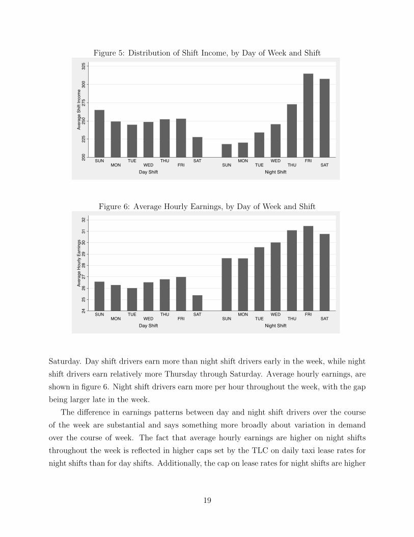
Figure 5: Distribution of Shift Income, by Day of Week and Shift
200
225
250
275
300
325
Aver
age
Shift
Inco
me
Day Shift Night Shift
SUNMON
TUEWED
THUFRI
SATSUN
MONTUE
WEDTHU
FRISAT
Figure 6: Average Hourly Earnings, by Day of Week and Shift
2425
2627
2829
3031
32Av
erag
e Ho
urly
Earn
ings
Day Shift Night Shift
SUNMON
TUEWED
THUFRI
SATSUN
MONTUE
WEDTHU
FRISAT
Saturday. Day shift drivers earn more than night shift drivers early in the week, while night
shift drivers earn relatively more Thursday through Saturday. Average hourly earnings, are
shown in figure 6. Night shift drivers earn more per hour throughout the week, with the gap
being larger late in the week.
The difference in earnings patterns between day and night shift drivers over the course
of the week are substantial and says something more broadly about variation in demand
over the course of week. The fact that average hourly earnings are higher on night shifts
throughout the week is reflected in higher caps set by the TLC on daily taxi lease rates for
night shifts than for day shifts. Additionally, the cap on lease rates for night shifts are higher
19

later in the week than earlier in the week.24
Given the sharp differences in labor supply and earnings patterns for day shift and night
shift drivers and the potential differences in available information regarding earnings oppor-
tunities when making labor supply decisions, I analyze the labor supply of day shift and
night shift drivers separately in what follows.
5.3 The CBLT Analysis
Because my analysis is meant as a replication and extension (with new data) of the analysis
of CBLT (1997), I start with a short summary of their analysis and results. CBLT base their
analysis of taxi driver labor supply on three samples:
1. TRIP – 70 shifts for 13 drivers (8 with multiple shifts) from April 24 - May 14, 1994.
2. TLC1 – 1044 shifts for 484 drivers (234 with multiple shifts) from October 29 - Novem-
ber 5, 1990.
3. TLC2 – 712 shifts for 712 drivers (none with multiple shifts) from November 1-3, 1988.
In the simplest terms, for each of their samples, CBLT regress log hours on a given shift
(defined as the difference in time between the drop-off time of the last fare and the pick-
up time of the first fare) on log average hourly earnings (defined as the ratio of total fare
income divided by hours worked). These regressions also control for other shift characteristics
including weekday vs. weekend, weather, day vs. night shift, and, in some specifications,
driver fixed effects. Presumably, day-to-day variation in hourly earnings controlling for the
other shift characteristics is the result of unanticipated transitory factors affecting earnings
opportunities. Using OLS, the estimated labor supply elasticities found by CBLT range from
-0.618 to -0.186, depending on sample used and other variables included in the model.
As CBLT recognize, the OLS estimate of the elasticity may well be downward biased due
to “division bias” if there is any specification or measurement error. This is because the key
explanatory variable, average hourly earnings, is calculated as the ratio of daily income to
daily hours and daily hours is the dependent variable. There are several reasons to suspect
measurement error. First, the data are imperfectly transcribed from potentially erroneous
hand recordings of trip sheets. Second, the trip sheets do not record tip income, which likely
24 The lease rate cap for day shifts has been $115 since October 2012. The lease rate cap for night shiftsvaries by day of week. The night shift cap since October 2012 ranges from $128 Sunday-Tuesday to $142Thursday-Saturday.
20
varies trip-to-trip around some mean tipping rate. Third, there may be breaks taken in the
middle of shifts that are not recorded as such. It is unclear how to handle these periods of
time in the data. And there are likely to be other sources of error.
CBLT address this problem in a sensible way by instrumenting for average hourly earnings
of a given driver with measures of the distribution of hourly earnings of other drivers on the
same calendar date. An obvious choice for an instrument for average hourly earnings is the
average log hourly earnings of other drivers on the same day, but this was not done. The
measures CBLT use as instruments are the 25th, 50th, and 75th percentiles of the other-
driver daily earnings distributions. One worry, particularly using the TRIP data, is that
there cannot be very many other drivers on any given day on which to base computation
of the instruments. Using their IV approach, CBLT find elasticities that are small and
insignificantly different from zero for the very small TRIP data but range from -1.313 to
-0.926 for the larger TCL1 and TCL2 samples. Interestingly, these IV elasticities are more
negative than those found using OLS.
5.4 New Estimates of the Labor Supply Elasticity
I begin by presenting OLS estimates of the labor supply elasticity based on the much larger
sample of over 5 million shifts from 2009-2013. These are regressions of log shift duration on
log average hourly earnings during the shift and other variables as noted below. I use four
samples: 1) all shifts, 2) day shifts, 3) night shifts, and 4) other (unclassified) shifts. These
samples are based on the 2/15 random sample of drivers described above, which includes
5,047,343 shifts for 8802 drivers over the 2009-2013 period. For each sample, I estimate
three specifications: 1) no controls, 2) a set of controls including indicators for day of week,
calendar week, year, the period subsequent to the September 4, 2012 fare increase, and
major holiday, and 3) additionally including driver fixed effects.25 These controls account
for anticipated wage variation and leave the average hourly earnings measure to account
for unanticipated transitory variation in earnings opportunities. I present the estimated
coefficient of log average hourly earnings, which is interpreted as the wage elasticity of labor
supply.
Table 4 contains these OLS estimates. The estimates for the entire sample, contained
in the first column of the table, show elasticities that are small and insignificantly different
from zero in the first two specifications. When driver fixed effects are included, the esti-
25 See footnote 17 for a list of major holidays used in defining the major-holiday indicator.
21
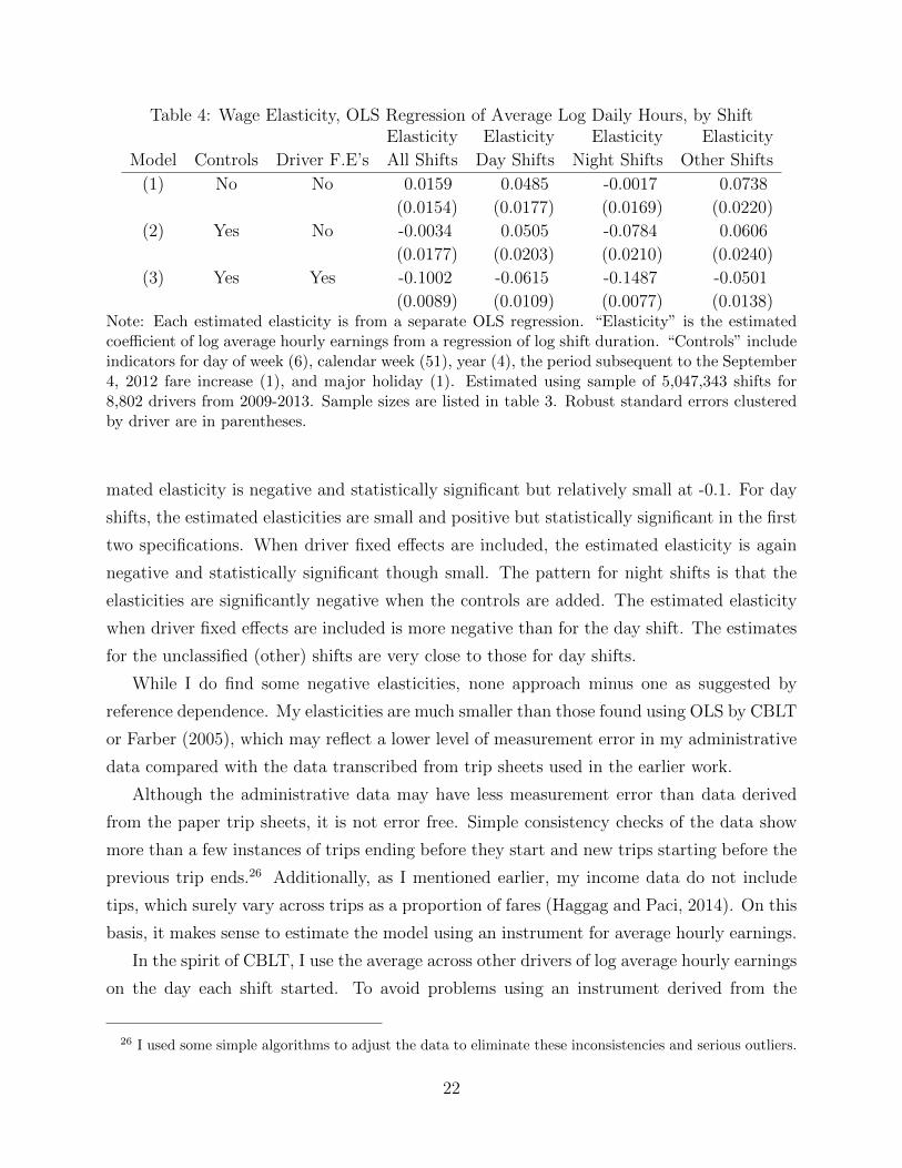
Table 4: Wage Elasticity, OLS Regression of Average Log Daily Hours, by ShiftElasticity Elasticity Elasticity Elasticity
Model Controls Driver F.E’s All Shifts Day Shifts Night Shifts Other Shifts
(1) No No 0.0159 0.0485 -0.0017 0.0738
(0.0154) (0.0177) (0.0169) (0.0220)
(2) Yes No -0.0034 0.0505 -0.0784 0.0606
(0.0177) (0.0203) (0.0210) (0.0240)
(3) Yes Yes -0.1002 -0.0615 -0.1487 -0.0501
(0.0089) (0.0109) (0.0077) (0.0138)Note: Each estimated elasticity is from a separate OLS regression. “Elasticity” is the estimatedcoefficient of log average hourly earnings from a regression of log shift duration. “Controls” includeindicators for day of week (6), calendar week (51), year (4), the period subsequent to the September4, 2012 fare increase (1), and major holiday (1). Estimated using sample of 5,047,343 shifts for8,802 drivers from 2009-2013. Sample sizes are listed in table 3. Robust standard errors clusteredby driver are in parentheses.
mated elasticity is negative and statistically significant but relatively small at -0.1. For day
shifts, the estimated elasticities are small and positive but statistically significant in the first
two specifications. When driver fixed effects are included, the estimated elasticity is again
negative and statistically significant though small. The pattern for night shifts is that the
elasticities are significantly negative when the controls are added. The estimated elasticity
when driver fixed effects are included is more negative than for the day shift. The estimates
for the unclassified (other) shifts are very close to those for day shifts.
While I do find some negative elasticities, none approach minus one as suggested by
reference dependence. My elasticities are much smaller than those found using OLS by CBLT
or Farber (2005), which may reflect a lower level of measurement error in my administrative
data compared with the data transcribed from trip sheets used in the earlier work.
Although the administrative data may have less measurement error than data derived
from the paper trip sheets, it is not error free. Simple consistency checks of the data show
more than a few instances of trips ending before they start and new trips starting before the
previous trip ends.26 Additionally, as I mentioned earlier, my income data do not include
tips, which surely vary across trips as a proportion of fares (Haggag and Paci, 2014). On this
basis, it makes sense to estimate the model using an instrument for average hourly earnings.
In the spirit of CBLT, I use the average across other drivers of log average hourly earnings
on the day each shift started. To avoid problems using an instrument derived from the
26 I used some simple algorithms to adjust the data to eliminate these inconsistencies and serious outliers.
22
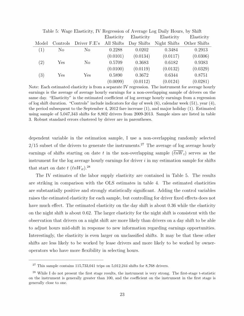
Table 5: Wage Elasticity, IV Regression of Average Log Daily Hours, by ShiftElasticity Elasticity Elasticity Elasticity
Model Controls Driver F.E’s All Shifts Day Shifts Night Shifts Other Shifts
(1) No No 0.2288 0.0202 0.3484 0.2913
(0.0101) (0.0134) (0.0117) (0.0306)
(2) Yes No 0.5709 0.3683 0.6182 0.9383
(0.0100) (0.0119) (0.0132) (0.0329)
(3) Yes Yes 0.5890 0.3672 0.6344 0.8751
(0.0099) (0.0112) (0.0124) (0.0281)Note: Each estimated elasticity is from a separate IV regression. The instrument for average hourlyearnings is the average of average hourly earnings for a non-overlapping sample of drivers on thesame day. “Elasticity” is the estimated coefficient of log average hourly earnings from a regressionof log shift duration. “Controls” include indicators for day of week (6), calendar week (51), year (4),the period subsequent to the September 4, 2012 fare increase (1), and major holiday (1). Estimatedusing sample of 5,047,343 shifts for 8,802 drivers from 2009-2013. Sample sizes are listed in table3. Robust standard errors clustered by driver are in parentheses.
dependent variable in the estimation sample, I use a non-overlapping randomly selected
2/15 subset of the drivers to generate the instruments.27 The average of log average hourly
earnings of shifts starting on date t in the non-overlapping sample (`nW t) serves as the
instrument for the log average hourly earnings for driver i in my estimation sample for shifts
that start on date t (`nWit).28
The IV estimates of the labor supply elasticity are contained in Table 5. The results
are striking in comparison with the OLS estimates in table 4. The estimated elasticities
are substantially positive and strongly statistically significant. Adding the control variables
raises the estimated elasticity for each sample, but controlling for driver fixed effects does not
have much effect. The estimated elasticity on the day shift is about 0.36 while the elasticity
on the night shift is about 0.62. The larger elasticity for the night shift is consistent with the
observation that drivers on a night shift are more likely than drivers on a day shift to be able
to adjust hours mid-shift in response to new information regarding earnings opportunities.
Interestingly, the elasticity is even larger on unclassified shifts. It may be that these other
shifts are less likely to be worked by lease drivers and more likely to be worked by owner-
operators who have more flexibility in selecting hours.
27 This sample contains 115,733,041 trips on 5,012,244 shifts for 8,768 drivers.
28 While I do not present the first stage results, the instrument is very strong. The first-stage t-statisticon the instrument is generally greater than 100, and the coefficient on the instrument in the first stage isgenerally close to one.
23
Overall, the evidence presented so far is consistent with the neoclassical optimizing model.
The positive estimated elasticities do not support the idea that taxi drivers have reference
dependent preferences and are target earners.
6 Does the Labor Supply Elasticity Depend on How
the Wage Compares With the Expected Wage?
The theoretical discussion in section 2 set bounds on the range within which one would
expect to find target earnings behavior (an elasticity of -1). If the realized daily wage lies
in the range defined by equations 11 and 12, then target earnings behavior will be observed.
Otherwise, the labor supply elasticity with respect to unanticipated transitory wage variation
will be positive. Intuitively, reference dependence is a local phenomenon. If the wage is far
lower than what was expected, drivers will find it optimal to stop working before the reference
income level is reached, and, if the wage is far higher than what was expected, drivers will
find it optimal to continue working after the reference income level is reached.
I calculate the expected log wage for each day using data on mean daily log average hourly
earnings for drivers in the non-overlapping sample that I used to construct the instrument for
the estimation of the labor supply model in section 5.4. The expected log wage is calculated
as the predicted value of log average hourly earnings from an OLS regression of the daily
average log average hourly earnings on indicators for day of week, week of year, year, the
period after the fare increase of September 4, 2012 and major holiday. I then calculate
the difference between the observed average daily log average hourly earnings in the non-
overlapping sample and the predicted value. This difference is what I use as the deviation
of the average daily log wage from its expectation.
Across the 1826 days in the sample from 2009-2013, the average deviation is zero by con-
struction. Interestingly, the deviations appear relatively small. The average of the absolute
deviation is 0.033, and the inter-quartile range of the absolute deviation runs from 0.011 to
0.043. The 90th percentile of the absolute deviation is 0.067 and the 95th percentile is 0.093.
In other words, less than 5 percent of the days considers have an observed deviation from
expected average hourly earnings of 10 percent or more.
The bounds on what is a sufficiently small deviation from the expected log wage are
defined in equations 11 and 12. These bounds depend on the importance of gain-loss utility
in the utility function (equations 1 and 2), which is controlled by the parameter α and by the
neoclassical labor supply elasticity, which is controlled by the parameter ν. The parameter
24
α is directly related to the coefficient of loss aversion (λ) used in the behavioral economics
literature. The coefficient of loss aversion is defined as the ratio of marginal utility below
the reference point to marginal utility above the reference point. In the utility specification
used here (equations 1 and 2), coefficient of loss aversion is λ = (1+α)(1−α) , which implies that
α = (λ−1)(λ+1)
.
Existing evidence, mostly from laboratory experiments suggests that the coefficient of
loss aversion is in the range of 1.5 to 2.5.29 This implies a range on the parameter α of 0.2
to 0.43. Assuming an elasticity of labor supply of 0.5, α of 0.2 (λ = 1.5) implies bounds of
`n(W ∗) = −0.15 and `n(W ∗∗) = 0.12. The larger value of α of 0.43 (λ = 2.5) implies wider
bounds: `n(W ∗) = −0.35 and `n(W ∗∗) = 0.24. A larger labor supply elasticity would lead
to wider bounds.
Even the narrower of the bounds I calculate here (-0.15 to +0.12) are quite substantial
relative to the observed range of unanticipated variation in daily average hourly earnings.
Only 28 of the 1826 days had unanticipated variation below -0.15 and only 11 of the 1826
days had unanticipated variation above 0.12. In other words, virtually all days (about 98
percent) saw unanticipated wage variation small enough to imply reference dependence and
target earnings behavior at these reasonable parameter values. Intuitively, since most of
the observed unanticipated variation in the wage is likely within the range where target
earnings behavior is relevant, strong hints of such behavior ought to be observed in the full
sample estimates, and the fact that the full-sample estimates of the labor supply elasticity
are strongly positive suggests that reference dependence is not playing a large role in taxi
driver labor supply.
These calculations not withstanding, I investigate how the estimated elasticity varies with
the daily level of unanticipated wage variation by estimating separate labor supply functions
for days where the deviation between average log hourly earnings and expected log average
hourly earnings is very small or is larger. I focus on days where the absolute deviation
between the average log wage and its expected value is below the median (0.0183434).30 My
view is that absolute deviations from the expected wage below this limit are so small relative
to the calculated bounds that they should provide the reference dependent preference model
29 See, for example, Tversky and Kahneman (1991) and Abdellaoui Bleichrodt and Paraschiv (2007). Arecent field study comparing taxes and bonuses as incentives for the use of reusable bags at supermarkets(Homonoff, 2014), finds a much higher value for λ of 5 or more in this low stakes setting.
30 The distribution considered uses the date the shift started as the operative date. No adjustment is madefor the fact that some shifts span calendar days, and the same distribution is used for all shifts, regardlessof whether they are day or night shifts.
25
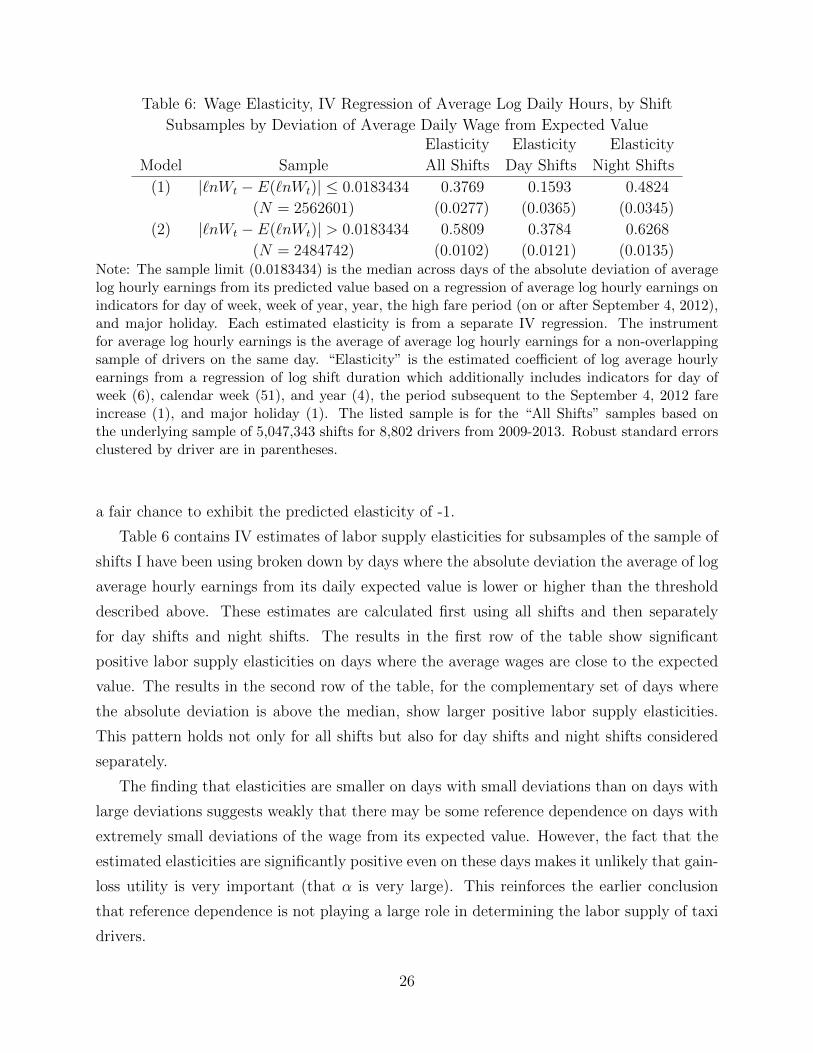
Table 6: Wage Elasticity, IV Regression of Average Log Daily Hours, by Shift
Subsamples by Deviation of Average Daily Wage from Expected ValueElasticity Elasticity Elasticity
Model Sample All Shifts Day Shifts Night Shifts
(1) |`nWt − E(`nWt)| ≤ 0.0183434 0.3769 0.1593 0.4824
(N = 2562601) (0.0277) (0.0365) (0.0345)
(2) |`nWt − E(`nWt)| > 0.0183434 0.5809 0.3784 0.6268
(N = 2484742) (0.0102) (0.0121) (0.0135)Note: The sample limit (0.0183434) is the median across days of the absolute deviation of averagelog hourly earnings from its predicted value based on a regression of average log hourly earnings onindicators for day of week, week of year, year, the high fare period (on or after September 4, 2012),and major holiday. Each estimated elasticity is from a separate IV regression. The instrumentfor average log hourly earnings is the average of average log hourly earnings for a non-overlappingsample of drivers on the same day. “Elasticity” is the estimated coefficient of log average hourlyearnings from a regression of log shift duration which additionally includes indicators for day ofweek (6), calendar week (51), and year (4), the period subsequent to the September 4, 2012 fareincrease (1), and major holiday (1). The listed sample is for the “All Shifts” samples based onthe underlying sample of 5,047,343 shifts for 8,802 drivers from 2009-2013. Robust standard errorsclustered by driver are in parentheses.
a fair chance to exhibit the predicted elasticity of -1.
Table 6 contains IV estimates of labor supply elasticities for subsamples of the sample of
shifts I have been using broken down by days where the absolute deviation the average of log
average hourly earnings from its daily expected value is lower or higher than the threshold
described above. These estimates are calculated first using all shifts and then separately
for day shifts and night shifts. The results in the first row of the table show significant
positive labor supply elasticities on days where the average wages are close to the expected
value. The results in the second row of the table, for the complementary set of days where
the absolute deviation is above the median, show larger positive labor supply elasticities.
This pattern holds not only for all shifts but also for day shifts and night shifts considered
separately.
The finding that elasticities are smaller on days with small deviations than on days with
large deviations suggests weakly that there may be some reference dependence on days with
extremely small deviations of the wage from its expected value. However, the fact that the
estimated elasticities are significantly positive even on these days makes it unlikely that gain-
loss utility is very important (that α is very large). This reinforces the earlier conclusion
that reference dependence is not playing a large role in determining the labor supply of taxi
drivers.
26
7 Do Different Drivers Use Different Models?
Economists typically assume a single model of behavior applies to all agents and estimate the
parameters of said model. The scale of the data available here makes it feasible to estimate
separate labor supply models for individual drivers. It may be that some drivers exhibit
reference dependent preferences (substantial negative labor supply elasticities) while others
are optimizers (positive labor supply elasticities).31
In this section, I estimate separate labor supply models by driver for the large number of
drivers who are observed on a substantial number of shifts. Given the difference in decision
making margins and estimated elasticities for day shifts and night shifts, I make a distinction
between “day shift drivers” and “night shift drivers.” Call drivers who work at least 750 day
shifts between 2009 and 2013 day shift drivers, and call drivers who work at least 750 night
shifts between 2009 and 2013 night shift drivers. There are 1267 day shift drivers and 1205
night shift drivers in the 2/15 random sample. While most drivers are observed working
different shifts over the period, drivers do tend to specialize. For example, there are only
two drivers who are classified as both day shift and night shift. The mean number of night
shifts for day shift drivers is 46.6 and the mean number of day shifts for night shift drivers
is 55.8. I proceed estimating separate labor supply models for the day shifts of the day shift
drivers and for the night shifts of the night shift drivers.
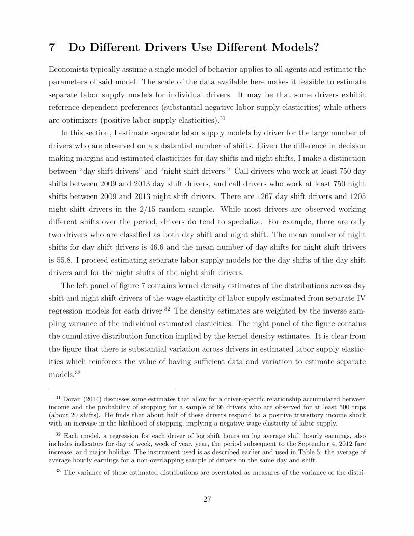
The left panel of figure 7 contains kernel density estimates of the distributions across day
shift and night shift drivers of the wage elasticity of labor supply estimated from separate IV
regression models for each driver.32 The density estimates are weighted by the inverse sam-
pling variance of the individual estimated elasticities. The right panel of the figure contains
the cumulative distribution function implied by the kernel density estimates. It is clear from
the figure that there is substantial variation across drivers in estimated labor supply elastic-
ities which reinforces the value of having sufficient data and variation to estimate separate
models.33
31 Doran (2014) discusses some estimates that allow for a driver-specific relationship accumulated betweenincome and the probability of stopping for a sample of 66 drivers who are observed for at least 500 trips(about 20 shifts). He finds that about half of these drivers respond to a positive transitory income shockwith an increase in the likelihood of stopping, implying a negative wage elasticity of labor supply.
32 Each model, a regression for each driver of log shift hours on log average shift hourly earnings, alsoincludes indicators for day of week, week of year, year, the period subsequent to the September 4, 2012 fareincrease, and major holiday. The instrument used is as described earlier and used in Table 5: the average ofaverage hourly earnings for a non-overlapping sample of drivers on the same day and shift.
33 The variance of these estimated distributions are overstated as measures of the variance of the distri-
27
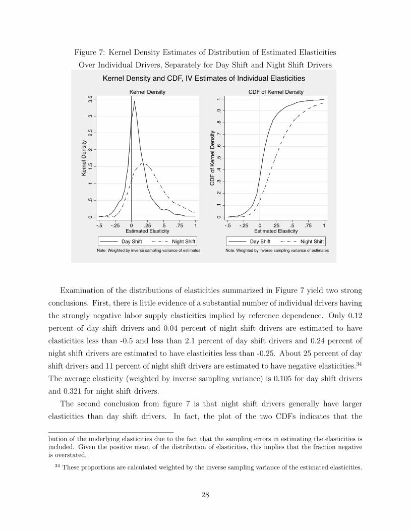
Figure 7: Kernel Density Estimates of Distribution of Estimated Elasticities
Over Individual Drivers, Separately for Day Shift and Night Shift Drivers
0.5
11.
52
2.5
33.
5
-.5 -.25 0 .25 .5 .75 1Estimated Elasticity
Day Shift Night Shift
Kern
el D
ensi
tyKernel Density
Note: Weighted by inverse sampling variance of estimates
0.1
.2.3
.4.5
.6.7
.8.9
1-.5 -.25 0 .25 .5 .75 1
Estimated Elasticity
Day Shift Night Shift
CD
F of
Ker
nel D
ensi
ty
CDF of Kernel Density
Note: Weighted by inverse sampling variance of estimates
Kernel Density and CDF, IV Estimates of Individual Elasticities
Examination of the distributions of elasticities summarized in Figure 7 yield two strong
conclusions. First, there is little evidence of a substantial number of individual drivers having
the strongly negative labor supply elasticities implied by reference dependence. Only 0.12
percent of day shift drivers and 0.04 percent of night shift drivers are estimated to have
elasticities less than -0.5 and less than 2.1 percent of day shift drivers and 0.24 percent of
night shift drivers are estimated to have elasticities less than -0.25. About 25 percent of day
shift drivers and 11 percent of night shift drivers are estimated to have negative elasticities.34
The average elasticity (weighted by inverse sampling variance) is 0.105 for day shift drivers
and 0.321 for night shift drivers.
The second conclusion from figure 7 is that night shift drivers generally have larger
elasticities than day shift drivers. In fact, the plot of the two CDFs indicates that the
bution of the underlying elasticities due to the fact that the sampling errors in estimating the elasticities isincluded. Given the positive mean of the distribution of elasticities, this implies that the fraction negativeis overstated.
34 These proportions are calculated weighted by the inverse sampling variance of the estimated elasticities.
28
distribution of elasticities for night shift drivers stochastically dominates the distribution
for day shift drivers. The generally larger elasticities for night shift drivers is consistent
with these drivers being more likely to be able to adjust hours to unanticipated changes in
earnings opportunities revealed during the shift. Note that with reference dependence, these
same considerations would imply that elasticities would be more strongly negative for night
shift drivers as they could work longer when wages are unexpectedly low in order to reach
the daily earnings reference point while drivers on day shifts may have more limited ability
to extend their shifts.
8 Do Drivers Learn to Optimize?
It is clear that optimizing behavior dominates reference dependence in the sense that in-
dividuals who set labor supply optimally will earn more money working fewer hours than
individuals who set labor supply as a result of reference dependence. Drivers who are op-
timizers will work relatively more hours on days when the wage is high, while drivers with
reference dependent preferences will work relatively more on days when the wage is low. It
may be that experience helps taxi drivers take advantage of high wage days, by teaching
them not only to behave as optimizers rather than target earners but also to take better
advantage of earnings opportunities by modifying their driving strategies.35
Given the importance of labor income and the time commitment of taxi drivers, the
value of learning how to optimize well is potentially very large in this industry.36 In order
to investigate the importance of learning, I analyze the labor supply of new taxi drivers and
how it changes as they accumulate experience. The first step is to identify new drivers. This
would be relatively straightforward if the actual hack license numbers of the drivers were
available since these numbers are assigned in sequence. However, the hack license numbers
are available only in encrypted form. As a result, I identify drivers as new if they were not
observed driving for some period from January 2009 forward.
In order to determine a reasonable period of non-observation to consider a driver a new
entrant, I analyzed the labor supply patterns over time in the 2/15 random subsample that I
35 Learning to be an optimizer is not a new idea. List (2003) studied two markets for collectibles andfound that experience resulted in a reduction in the importance of the endowment effect. This is related toreference dependence in that both the endowment effect and reference dependence flow from loss aversion.
36 Haggag, McManus, and Paci (2014) find substantial learning among New York City taxi drivers abouthow to find fares efficiently.
29
relied on above. It turns out that there is a fair amount of entry, exit, and reentry among taxi
drivers. For example, about 27 percent of the 8802 drivers in my sample did not drive for at
least one three-month period and then returned to driving. About 14 percent did not drive
for a six-month period and returned to driving. After not driving for a year, about 5 percent
of drivers returned, after 18 months of not driving about 3 percent of drivers returned, and
after two year of not driving, about 1.5 percent of drivers returned.
Conservatively, I define new drivers to be those are not observed driving for a full year
at the start of my data. In other words, while my data start in January 2009, I use the
2009 data only to identify drivers who are observed driving at some point in the 2010-2013
period but did not drive in 2009. Without a better method to identity new drivers, I live
with the likelihood that about 5 percent of drivers I classify as new are, in fact, experienced
to a greater or lesser extent. The restriction to drivers who did not have any shifts in 2009
eliminates about 64 percent of drivers and about 87 percent of shifts. In order to ensure a
sufficient sample, I use the full sample of drivers who did not have any shifts in 2009 for this
analysis, rather than only those in the 2/15 random subsample I have been using.
The sample of new entrants contains 4,814,278 shifts for 24,114 drivers. However, fully
7,038 (29 percent) of these drivers are observed for only a single shift, and 4,555 of these
single shifts have only a single trip. While it is possible that 29 percent of new drivers go
through the procedure of getting a hack license only to quit after a single trip or shift, it
may also be that these are simply data anomalies. In what follows, I delete the 7,038 drivers
and their associated 7,038 shifts from the analysis. The remaining analysis sample contains
4,807,240 shifts for 17,076 drivers.
I define experience based on number of shifts driven rather than by the passage of time,
and I divide experience into ten categories. I then estimate separate labor supply models for
each of the ten categories. Table 7 contains average characteristics of shifts by experience
category. There are some interesting patterns. Average hours worked increases early with
experience (from weeks 1 to 3) then declines after 6 months. Income per shift increases
sharply between weeks 1 and 2 and continues to increase as experience accumulates. Average
hourly earnings increases sharply with experience, by about 22 percent between the first
week and year 3 or later. Finally, it appears that new drivers are relatively more likely than
more experienced drivers to be on day shifts and, conversely, more experienced drivers are
relatively more likely than less experienced drivers to be on night shifts. As the data in figure
6 show, average hourly earnings are higher on night shifts, but further analysis (not shown
here) suggests that movement toward night shifts accounts for very little of the growth in
30
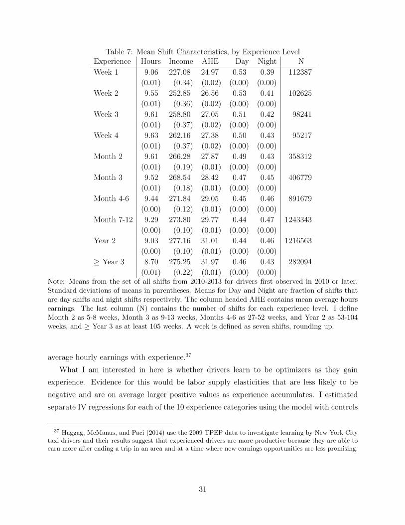
Table 7: Mean Shift Characteristics, by Experience LevelExperience Hours Income AHE Day Night N
Week 1 9.06 227.08 24.97 0.53 0.39 112387
(0.01) (0.34) (0.02) (0.00) (0.00)
Week 2 9.55 252.85 26.56 0.53 0.41 102625
(0.01) (0.36) (0.02) (0.00) (0.00)
Week 3 9.61 258.80 27.05 0.51 0.42 98241
(0.01) (0.37) (0.02) (0.00) (0.00)
Week 4 9.63 262.16 27.38 0.50 0.43 95217
(0.01) (0.37) (0.02) (0.00) (0.00)
Month 2 9.61 266.28 27.87 0.49 0.43 358312
(0.01) (0.19) (0.01) (0.00) (0.00)
Month 3 9.52 268.54 28.42 0.47 0.45 406779
(0.01) (0.18) (0.01) (0.00) (0.00)
Month 4-6 9.44 271.84 29.05 0.45 0.46 891679
(0.00) (0.12) (0.01) (0.00) (0.00)
Month 7-12 9.29 273.80 29.77 0.44 0.47 1243343
(0.00) (0.10) (0.01) (0.00) (0.00)
Year 2 9.03 277.16 31.01 0.44 0.46 1216563
(0.00) (0.10) (0.01) (0.00) (0.00)
≥ Year 3 8.70 275.25 31.97 0.46 0.43 282094
(0.01) (0.22) (0.01) (0.00) (0.00)Note: Means from the set of all shifts from 2010-2013 for drivers first observed in 2010 or later.Standard deviations of means in parentheses. Means for Day and Night are fraction of shifts thatare day shifts and night shifts respectively. The column headed AHE contains mean average hoursearnings. The last column (N) contains the number of shifts for each experience level. I defineMonth 2 as 5-8 weeks, Month 3 as 9-13 weeks, Months 4-6 as 27-52 weeks, and Year 2 as 53-104weeks, and ≥ Year 3 as at least 105 weeks. A week is defined as seven shifts, rounding up.
average hourly earnings with experience.37
What I am interested in here is whether drivers learn to be optimizers as they gain
experience. Evidence for this would be labor supply elasticities that are less likely to be
negative and are on average larger positive values as experience accumulates. I estimated
separate IV regressions for each of the 10 experience categories using the model with controls
37 Haggag, McManus, and Paci (2014) use the 2009 TPEP data to investigate learning by New York Citytaxi drivers and their results suggest that experienced drivers are more productive because they are able toearn more after ending a trip in an area and at a time where new earnings opportunities are less promising.
31
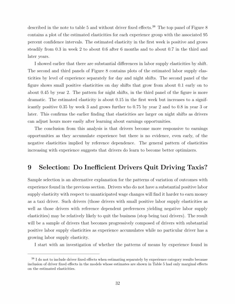
described in the note to table 5 and without driver fixed effects.38 The top panel of Figure 8
contains a plot of the estimated elasticities for each experience group with the associated 95
percent confidence intervals. The estimated elasticity in the first week is positive and grows
steadily from 0.3 in week 2 to about 0.6 after 6 months and to about 0.7 in the third and
later years.
I showed earlier that there are substantial differences in labor supply elasticities by shift.
The second and third panels of Figure 8 contains plots of the estimated labor supply elas-
ticities by level of experience separately for day and night shifts. The second panel of the
figure shows small positive elasticities on day shifts that grow from about 0.1 early on to
about 0.45 by year 2. The pattern for night shifts, in the third panel of the figure is more
dramatic. The estimated elasticity is about 0.15 in the first week but increases to a signif-
icantly positive 0.35 by week 3 and grows further to 0.75 by year 2 and to 0.8 in year 3 or
later. This confirms the earlier finding that elasticities are larger on night shifts as drivers
can adjust hours more easily after learning about earnings opportunities.
The conclusion from this analysis is that drivers become more responsive to earnings
opportunities as they accumulate experience but there is no evidence, even early, of the
negative elasticities implied by reference dependence. The general pattern of elasticities
increasing with experience suggests that drivers do learn to become better optimizers.
9 Selection: Do Inefficient Drivers Quit Driving Taxis?
Sample selection is an alternative explanation for the patterns of variation of outcomes with
experience found in the previous section. Drivers who do not have a substantial positive labor
supply elasticity with respect to unanticipated wage changes will find it harder to earn money
as a taxi driver. Such drivers (those drivers with small positive labor supply elasticities as
well as those drivers with reference dependent preferences yielding negative labor supply
elasticities) may be relatively likely to quit the business (stop being taxi drivers). The result
will be a sample of drivers that becomes progressively composed of drivers with substantial
positive labor supply elasticities as experience accumulates while no particular driver has a
growing labor supply elasticity.
I start with an investigation of whether the patterns of means by experience found in
38 I do not to include driver fixed effects when estimating separately by experience category results becauseinclusion of driver fixed effects in the models whose estimates are shown in Table 5 had only marginal effectson the estimated elasticities.
32
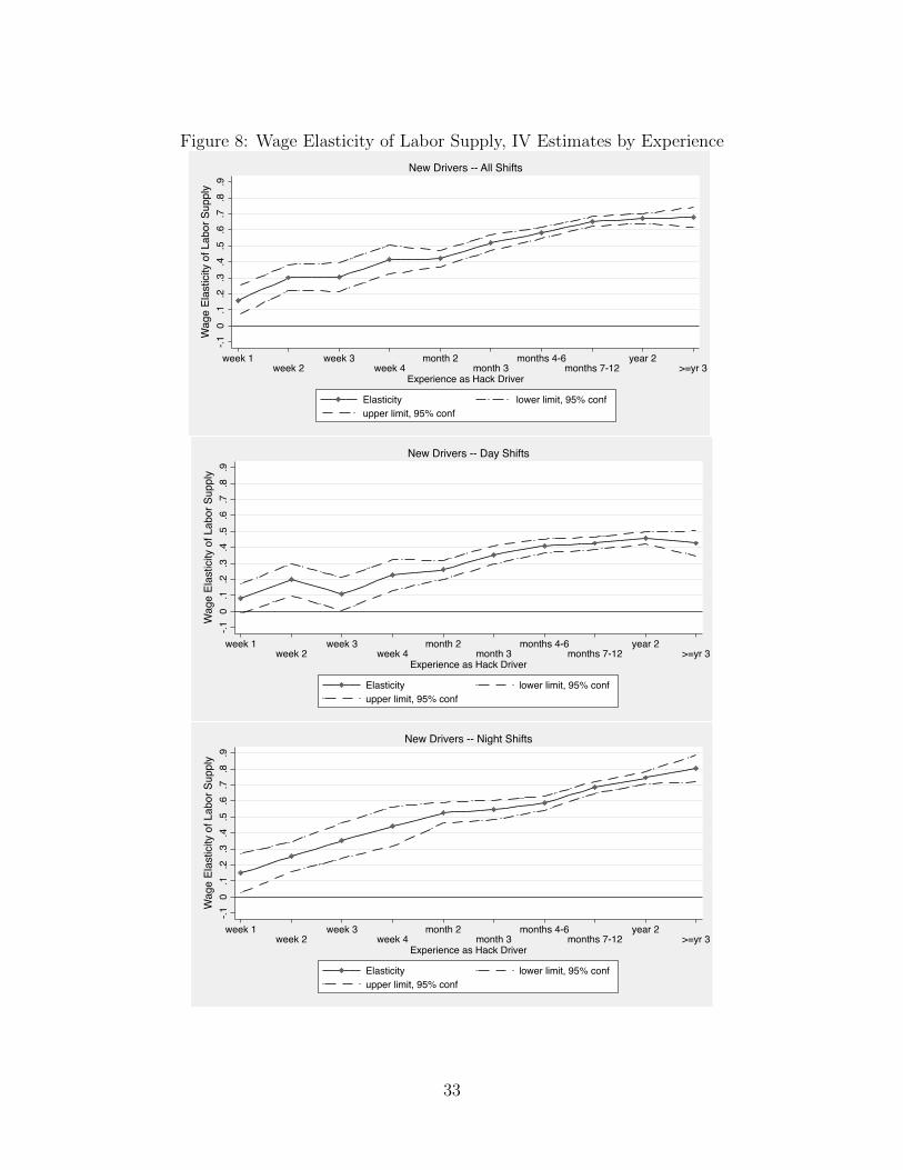
Figure 8: Wage Elasticity of Labor Supply, IV Estimates by Experience
-.10
.1.2
.3.4
.5.6
.7.8
.9
week 1week 2
week 3week 4
month 2month 3
months 4-6months 7-12
year 2>=yr 3
Experience as Hack Driver
Elasticity lower limit, 95% confupper limit, 95% conf
Wag
e El
astic
ity o
f Lab
or S
uppl
y
New Drivers -- All Shifts
-.10
.1.2
.3.4
.5.6
.7.8
.9
week 1week 2
week 3week 4
month 2month 3
months 4-6months 7-12
year 2>=yr 3
Experience as Hack Driver
Elasticity lower limit, 95% confupper limit, 95% conf
Wag
e El
astic
ity o
f Lab
or S
uppl
y
New Drivers -- Day Shifts
-.10
.1.2
.3.4
.5.6
.7.8
.9
week 1week 2
week 3week 4
month 2month 3
months 4-6months 7-12
year 2>=yr 3
Experience as Hack Driver
Elasticity lower limit, 95% confupper limit, 95% conf
Wag
e El
astic
ity o
f Lab
or S
uppl
y
New Drivers -- Night Shifts
33
Table 8: Mean Shift Characteristics, by Experience Level
Drivers with more than 52 Weeks Total Driving ExperienceExperience Hours Income AHE Day Night N
Week 1 9.31 222.65 23.90 0.55 0.39 35597
(0.02) (0.57) (0.03) (0.00) (0.00)
Week 2 9.69 243.89 25.30 0.54 0.41 35597
(0.02) (0.57) (0.03) (0.00) (0.00)
Week 3 9.72 248.99 25.75 0.52 0.42 35597
(0.02) (0.57) (0.03) (0.00) (0.00)
Week 4 9.81 253.76 26.06 0.51 0.43 35597
(0.02) (0.57) (0.03) (0.00) (0.00)
Month 2 9.75 256.73 26.53 0.50 0.43 150388
(0.01) (0.29) (0.02) (0.00) (0.00)
Month 3 9.61 258.36 27.07 0.48 0.44 187985
(0.01) (0.26) (0.02) (0.00) (0.00)
Month 4-6 9.48 262.87 27.96 0.47 0.45 488761
(0.01) (0.16) (0.01) (0.00) (0.00)
Month 7-12 9.29 270.78 29.45 0.44 0.46 977522
(0.00) (0.11) (0.01) (0.00) (0.00)
Year 2 9.03 277.16 31.01 0.44 0.46 1216563
(0.00) (0.10) (0.01) (0.00) (0.00)
≥ Year 3 8.70 275.25 31.97 0.46 0.43 282094
(0.01) (0.21) (0.01) (0.00) (0.00)Note: Means from set of all shifts from 2010-2013 for drivers with more than 52 weeks total drivingexperience first observed in 2010 or later. Standard deviations of means in parentheses. See noteto table 7 for detailed definitions.
table 7 are due to systematic exit of drivers at low levels of experience. In order to explore
this possibility, table 8 contains mean shift characteristics by experience for the subsample of
drivers who are first observed in 2010 and have more than 52 weeks total driving experience.
This subsample has 3,453,701 shifts for 5,371 drivers. The general pattern of variation of
each outcome with experience for this sample of very experienced drivers is identical to that
for the sample of all drivers shown in table 7. This is evidence that systematic exit from
the industry is not driving the patterns seen in table 7, and the fact that average hourly
earnings is growing with experience suggests that drivers do learn with experience.
The key question is whether or not drivers who exit early have negative or smaller positive
labor supply elasticities than do drivers who do not exit early, and I turn now to an analysis
of that question. I define exit understanding that a gap in driving does not necessarily imply
34
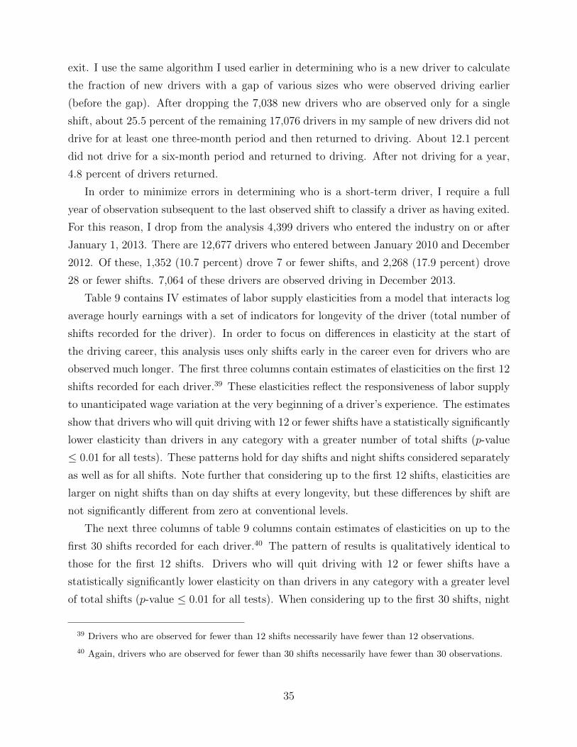
exit. I use the same algorithm I used earlier in determining who is a new driver to calculate
the fraction of new drivers with a gap of various sizes who were observed driving earlier
(before the gap). After dropping the 7,038 new drivers who are observed only for a single
shift, about 25.5 percent of the remaining 17,076 drivers in my sample of new drivers did not
drive for at least one three-month period and then returned to driving. About 12.1 percent
did not drive for a six-month period and returned to driving. After not driving for a year,
4.8 percent of drivers returned.
In order to minimize errors in determining who is a short-term driver, I require a full
year of observation subsequent to the last observed shift to classify a driver as having exited.
For this reason, I drop from the analysis 4,399 drivers who entered the industry on or after
January 1, 2013. There are 12,677 drivers who entered between January 2010 and December
2012. Of these, 1,352 (10.7 percent) drove 7 or fewer shifts, and 2,268 (17.9 percent) drove
28 or fewer shifts. 7,064 of these drivers are observed driving in December 2013.
Table 9 contains IV estimates of labor supply elasticities from a model that interacts log
average hourly earnings with a set of indicators for longevity of the driver (total number of
shifts recorded for the driver). In order to focus on differences in elasticity at the start of
the driving career, this analysis uses only shifts early in the career even for drivers who are
observed much longer. The first three columns contain estimates of elasticities on the first 12
shifts recorded for each driver.39 These elasticities reflect the responsiveness of labor supply
to unanticipated wage variation at the very beginning of a driver’s experience. The estimates
show that drivers who will quit driving with 12 or fewer shifts have a statistically significantly
lower elasticity than drivers in any category with a greater number of total shifts (p-value
≤ 0.01 for all tests). These patterns hold for day shifts and night shifts considered separately
as well as for all shifts. Note further that considering up to the first 12 shifts, elasticities are
larger on night shifts than on day shifts at every longevity, but these differences by shift are
not significantly different from zero at conventional levels.
The next three columns of table 9 columns contain estimates of elasticities on up to the
first 30 shifts recorded for each driver.40 The pattern of results is qualitatively identical to
those for the first 12 shifts. Drivers who will quit driving with 12 or fewer shifts have a
statistically significantly lower elasticity on than drivers in any category with a greater level
of total shifts (p-value ≤ 0.01 for all tests). When considering up to the first 30 shifts, night
39 Drivers who are observed for fewer than 12 shifts necessarily have fewer than 12 observations.
40 Again, drivers who are observed for fewer than 30 shifts necessarily have fewer than 30 observations.
35
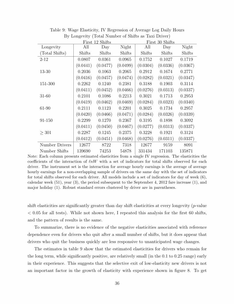
Table 9: Wage Elasticity, IV Regression of Average Log Daily Hours
By Longevity (Total Number of Shifts as Taxi Driver)
First 12 Shifts First 30 ShiftsLongevity All Day Night All Day Night
(Total Shifts) Shifts Shifts Shifts Shifts Shifts Shifts
2-12 0.0807 0.0361 0.0965 0.1752 0.1027 0.1719
(0.0441) (0.0477) (0.0499) (0.0304) (0.0336) (0.0367)
13-30 0.2036 0.1063 0.2065 0.2912 0.1674 0.2771
(0.0416) (0.0457) (0.0474) (0.0282) (0.0321) (0.0347)
151-300 0.2262 0.1240 0.2381 0.3188 0.1903 0.3114
(0.0411) (0.0452) (0.0466) (0.0276) (0.0313) (0.0337)
31-60 0.2101 0.1086 0.2213 0.3021 0.1713 0.2953
(0.0419) (0.0462) (0.0469) (0.0284) (0.0323) (0.0340)
61-90 0.2111 0.1123 0.2201 0.3025 0.1734 0.2957
(0.0420) (0.0466) (0.0471) (0.0284) (0.0326) (0.0339)
91-150 0.2299 0.1270 0.2367 0.3195 0.1898 0.3092
(0.0411) (0.0450) (0.0467) (0.0277) (0.0313) (0.0337)
≥ 301 0.2287 0.1245 0.2375 0.3228 0.1921 0.3124
(0.0412) (0.0451) (0.0468) (0.0276) (0.0311) (0.0337)
Number Drivers 12677 8722 7318 12677 9159 8091
Number Shifts 139690 74253 54878 331434 171103 135871Note: Each column presents estimated elasticities from a single IV regression. The elasticities thecoefficients of the interaction of `nW with a set of indicators for total shifts observed for eachdriver. The instrument set is the interaction for average hourly earnings is the average of averagehourly earnings for a non-overlapping sample of drivers on the same day with the set of indicatorsfor total shifts observed for each driver. All models include a set of indicators for day of week (6),calendar week (51), year (3), the period subsequent to the September 4, 2012 fare increase (1), andmajor holiday (1). Robust standard errors clustered by driver are in parentheses.
shift elasticities are significantly greater than day shift elasticities at every longevity (p-value
< 0.05 for all tests). While not shown here, I repeated this analysis for the first 60 shifts,
and the pattern of results is the same.
To summarize, there is no evidence of the negative elasticities associated with reference
dependence even for drivers who quit after a small number of shifts, but it does appear that
drivers who quit the business quickly are less responsive to unanticipated wage changes.
The estimates in table 9 show that the estimated elasticities for drivers who remain for
the long term, while significantly positive, are relatively small (in the 0.1 to 0.25 range) early
in their experience. This suggests that the selective exit of low-elasticity new drivers is not
an important factor in the growth of elasticity with experience shown in figure 8. To get
36

at this directly, I computed IV estimates of the wage elasticities by experience for longer-
term drivers. To identify a group of longer-term drivers, I note that most exit happens very
quickly, with 12 percent driving 7 or fewer shifts, 15.6 percent driving 12 or fewer shifts, and
22 percent driving 28 or fewer shifts.41 The rate of exit slows down substantially after 28
shifts, and I use this value to demarcate longer-term drivers.
The top panel of figure 9 shows IV estimates of the wage elasticities by experience for
longer-term drivers, defined as those who are observed to drive more than 28 shifts. These
estimates shows the same pattern of increasing labor supply elasticity as was seen in figure 8.
The second and third panels of figure 9 contain plots of the estimated labor supply elasticities
by level of experience separately for day and night shifts. The general pattern is the same
as is shown in figure 8 for the combination of long-term and short-term drivers. Elasticities
grow with experience for both day shift drivers and night shift drivers, but they grow more
rapidly for night shift workers and wind up at a much higher level. These estimates support
the conclusion that drivers, in fact, learn to optimize and that the increase in elasticity with
experience is not an artifact of selection.
To summarize, there is clear evidence that drivers with low labor supply elasticity tend
to exit the industry early. Short-term drivers exhibit significantly lower elasticity of labor
supply than do long-term drivers at the same (low) level of experience. The evidence on
long-term drivers, that the labor supply elasticity grows with experience over the first few
years of driving, is consistent with the view that these drivers learn to optimize over time
by learning (how) to adjust their daily labor supply positively in response to unanticipated
variation in daily earnings opportunities. There is no evidence in these data that drivers,
either those who exit early or those who are longer-term, exhibit reference dependence in
their labor supply decisions.
10 Final Remarks
Following on the work of Camerer, Babcock, Loewenstein, and Thaler (1997), I evaluated
the role of reference dependence vs neoclassical optimizing behavior in determining daily
hours decisions of taxi driver in New York City using the complete driving records of all
NYC taxi drivers over the 2009-2013 period. The high-level conclusion is that there is little
evidence that reference dependence is an important factor determining the labor supply of
41 This tabulation is based on the 17,076 new drivers who drive for more than a single shift. The 7,038drivers who are observed for a single shift are not considered.
37
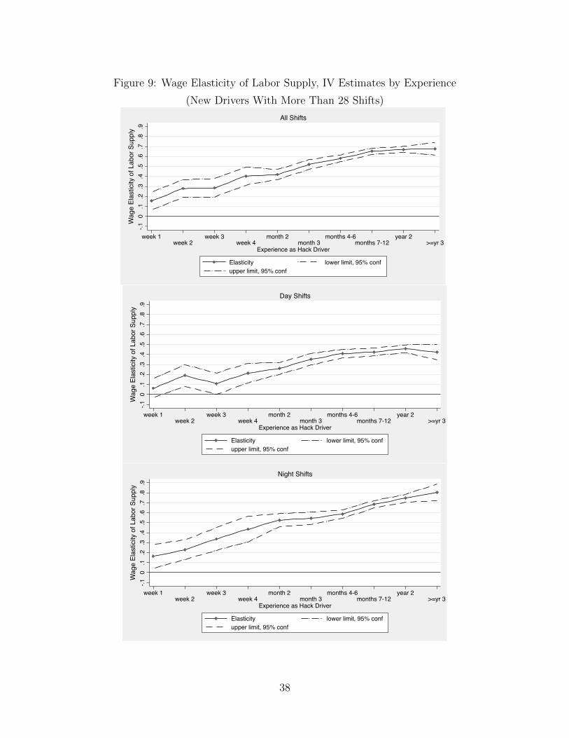
Figure 9: Wage Elasticity of Labor Supply, IV Estimates by Experience
(New Drivers With More Than 28 Shifts)
-.10
.1.2
.3.4
.5.6
.7.8
.9
week 1week 2
week 3week 4
month 2month 3
months 4-6months 7-12
year 2>=yr 3
Experience as Hack Driver
Elasticity lower limit, 95% confupper limit, 95% conf
Wag
e El
astic
ity o
f Lab
or S
uppl
y
All Shifts
-.10
.1.2
.3.4
.5.6
.7.8
.9
week 1week 2
week 3week 4
month 2month 3
months 4-6months 7-12
year 2>=yr 3
Experience as Hack Driver
Elasticity lower limit, 95% confupper limit, 95% conf
Wag
e El
astic
ity o
f Lab
or S
uppl
y
Day Shifts
-.10
.1.2
.3.4
.5.6
.7.8
.9
week 1week 2
week 3week 4
month 2month 3
months 4-6months 7-12
year 2>=yr 3
Experience as Hack Driver
Elasticity lower limit, 95% confupper limit, 95% conf
Wag
e El
astic
ity o
f Lab
or S
uppl
y
Night Shifts
38

NYC taxi drivers. This conclusion rests on several pieces of evidence:
• Koszegi and Rabin’s (2006) model of expectations-based reference points implies that
reference dependence is relevant only for unanticipated wage movements in the wage.
However, only about one-eighth of total hourly wage variation is unanticipated. Thus,
most variation in wages (the seven-eighths that is anticipated) affects labor supply
neoclassically.
• Instrumental variable estimates of labor supply elasticities, based on a very large sam-
ple of about 5 million shifts for 8,802 drivers, are strongly positive and range from 0.4
to 0.8, depending on shift. There is no evidence of negative labor supply elasticities or
target earnings behavior (a prediction of the reference dependence model).
• The model further predicts that reference dependence will be relevant when unan-
ticipated transitory wage variation is small and not relevant when this variation is
large. However, there is no evidence of target earnings behavior even on days where
unanticipated wage variation is very small.
• Allowing individual drivers to have their own labor supply elasticities yields a range of
estimated elasticities of labor supply, but the large majority of elasticities are estimated
to be positive, and only a tiny fraction of drivers are estimated to have substantial
negative elasticities.
Behaving as a target earner is an inefficient way to earn money. Important questions are
1) whether new drivers learn to take advantage of strong earnings opportunities by working
more on high wage days and less on low wage days and 2) whether new drivers who start with
negative or small positive labor supply elasticities quit the business. The answer to both
questions is yes. The estimated labor supply elasticity grows substantially with experience,
and new drivers with small labor supply elasticities are more likely to quit. Those who
remain have growing elasticity with experience. In other words, new drivers who continue in
the industry learn how to be better optimizers (respond more positively to wage variation).
There is no evidence of negative labor supply elasticities for new drivers even at the start.
To summarize, the overall pattern is clear. Drivers tend to respond positively to both
anticipated and unanticipated increases in earnings opportunities. This is consistent with
the neoclassical optimizing model of labor supply, and I conclude that reference dependence
does not play an important role in determining the labor supply of taxi drivers in New York
City.
39
References
Abdellaoui, Mohammed, Han Bleichrodt, and Corina Paraschiv. “Loss Aversion under
Prospect Theory: A Parameter-Free Measurement,” Management Science 53(10) (Oc-
tober 2007) pp. 1659-1674.
Abeler, Johannes, Armin Falk, Lorenz Goette, and David Huffman. “Reference Points and
Effort Provision,” American Economic Review 101(2) (2011) pp. 470-92
Agarwal, Sumit; Mio Diao; Jessica Pan; and Tien Foo Sing, “Labor Supply Decisions of
Singaporean Cab Drivers,” mimeo, University of Singapore, October 2013.
Ashenfelter, Orley, Kirk Doran, and Bruce Schaller. “A Shred of Credible Evidence on the
Long-run Elasticity of Labour Supply,” Economica 77 (2010) pp. 637-650.
Blundell, Richard and Thomas MaCurdy. “Labor Supply: A Review of Alternative Ap-
proaches,” in Handbook of Labor Economics, O. Ashenfelter and D. Card, eds. Ams-
terdam, North Holland, vol 3a. 1986: pp. 1559-1695.
Camerer, Colin, “Taxi Drivers and Beauty Contests.” Engineering & Science, California
Institute of Technology, 1997, pp. 10-19.
Camerer, Colin.”Prospect Theory in the Wild: Evidence from the Field,” in Choices, Values,
and Frames. D. Kahneman adn A. Tversky, eds. Cambridge UK: Cambridge University
Press, 2000, pp. 288-300.
Camerer, Colin; Linda Babcock; George Loewenstein; and Richard Thaler, “Labor Supply
of New York City Cabdrivers: One Day at a Time,” Quarterly Journal of Economics
112 (May 1997), pp. 407 – 441.
Chou, Yuan K. “Testing Alternative Models of Labor Supply: Evidence from Taxi Drivers
in Singapore.” The Singapore Economic Review 47 (2002).
Crawford, Vincent P. and Juanjuan Meng. “New York City Cab Drivers Labor Supply
Revisited: Reference-Dependent Preference with Rational Expectations Targets for
Hours and Income,” American Economic Review 101 (2011) pp. 1912-1932.
Doran, Kirk. “Are Long-Term Wage Elasticities of Labor Supply More Negative than Short-
Term Ones?” Economic Letters 122 (2014) pp. 208-210.
Farber, Henry S. “Is Tomorrow Another Day? The Labor Supply of New York City Cab
Drivers,” Journal of Political Economy 113 (February 2005), pp. 46-82.
40
Farber, Henry S. “Reference-Dependent Preferences and Labor Supply: The Case of New
York City Taxi Drivers,” American Economic Review 98 (June 2008), pp. 1069-1082.
Fehr, Ernst and Lorenz Goette. “Do Workers Work More if Wages are High? Evidence
from a Randomized Field Experiment,” American Economic Review, 97(1) (2007) pp.
298-317.
Haggag, Kareem, Brian McManus, and Giovanni Paci. “Learning by Driving: Productiv-
ity Improvements by New York City Taxi Drivers.” June 2014. Available at SSRN:
http://ssrn.com/abstract=2456733.
Haggag, Kareem and Giovanni Paci. “Default Tips.” American Economic Journal: Applied
Economics 6(3) (July 2014): pp. 1-19.
Homonoff, Tatiana. “Can Small Incentives Have Large Effects? The Impact of Taxes versus
Bonuses on Disposable Bag Use.” Working Paper No. 575, Industrial Relations Section,
Princeton University, March 2013.
(Online at http://arks.princeton.edu/ark:/88435/dsp014q77fr47j).
Koszegi, Botond and Matthew Rabin. “A Model of Reference-Dependent Preferences,”
Quarterly Journal of Economics 121 (November 2006), pp. 1133-1165.
List, John A. “Does Market Experience Eliminate Market Anomolies?” Quarterly Journal
of Economics 118 (February 2003), pp. 41 – 71.
MaCurdy, Thomas E. “An Empirical Model of Labor Supply in a Life-Cycle Setting.” Jour-
nal of Political Economy 89 (December 1981): 1059-1085.
Nguyen, Quang and Pingsun Leung. “Revenue Targeting in Fisheries: The Case of Hawaii
Longline Fishery,” MPRA Paper No. 13846, March 7, 2009.
(Online at http://mpra.ub.uni-muenchen.de/13846).
Oettinger, Gerald S. “An Empirical Analysis of the Daily Labor Supply of Stadium Vendors,”
Journal of Political Economy 107 (April 1999), pp. 360-392.
Ordonez, Lisa; Maurice E. Schweitzer; Adam D. Galinsky, and and Max H. Bazerman “Goals
Gone Wild: The Systematic Side Effects of Over-Prescribing Goal Setting,” Academy
of Management Perspectives (February 2009), pp. 6-16.
Tversky, Amos and Daniel Kahneman. “Loss Aversion in Riskless Choice: A Reference-
Dependent Model,” Quarterly Journal of Economics 106 (November 1991), 1039-1061.
41