ISSN 0956-8549-754

Informational Black Holes in Financial Markets

By

Ulf Axelson and Igor Makarov

DISCUSSION PAPER NO 754

DISCUSSION PAPER SERIES

April 2016

1

Informational Black Holes in Financial Markets

Ulf Axelson Igor Makarov∗

April 22, 2016

ABSTRACT

We study how efficient primary financial markets are in allocating capital when information about investment opportunities is dispersed across market participants. Paradoxically, the very fact that information is valuable for making real investment decisions destroys the efficiency of the market. To add to the paradox, as the number of market participants with useful information increases a growing share of them fall into an “informational black hole,” making markets even less efficient. Contrary to the predictions of standard theory, social surplus and the revenues of an entrepreneur seeking financing can be decreasing in the size of the financial market, the linkage principle of Milgrom and Weber (1982) may not hold, and collusion among investors may enhance efficiency. JEL Codes: D44, D82, G10, G20.

∗London School of Economics. We thank Philip Bond, James Dow, Mehmet Ekmekci, Alexander Gorbenko, Andrey Malenko, Tom Noe, James Thompson, Vish Viswanathan, John Zhu, and seminar participants at Cass Business School, Cheung Kong GSB, Chicago Booth, INSEAD, London School of Economics, Stockholm School of Economics, Toulouse School of Economics, UBC, Univeristy of Oxford, University of Reading, the CEPR Gerzensee 2015 corporate finance meetings, European Winter Finance Conference 2015, the 2015 NBER Asset Pricing summer meetings, the 2015 NBER Corporate Finance fall meetings, the 2015 NBER fall entrepreneurship meetings, the 2015 OxFit meetings, the 12th Finance Theory Group meeting, the Financial Intermediation Research Society Conference 2015 (Reykjavik), and the Western Finance Association 2015 Seattle meetings for very helpful comments. Corresponding author, Ulf Axelson: London School of Economics, Houghton Street London, WC2A 2AE, UK; email: u.axelson@lse.ac.uk.

1

The main role of primary financial markets is to channel resources to firms with worth- while projects. This process requires information about demand, technological feasi- bility, management, and current industry and macroeconomic conditions, as well as views on how to interpret such information. No single investor typically holds all this information. The unprecedent growth of the financial sector over the last three decades has led to a proliferation of informed intermediaries such as venture capitalists, private equity firms, hedge funds, as well as fintech innovations such as peer-to-peer lending and crowdfunding platforms. As a result, although the amount of information about investment opportunities may have increased, it may have become more dispersed than ever.

In this paper, we ask two central questions about the functioning of primary finan- cial markets when information is dispersed: does market competition for the financing of new ventures lead to the right investment decision, and do larger markets lead to a more efficient outcome?

Based on the seminal work of Hayek (1945) and the follow-on literature, one would be tempted to answer “Yes” to both questions. Hayek argued that exactly in situations when information is dispersed, competitive markets are superior to centralized decision making because of the ability of markets to aggregate information—the “wisdom of the crowd” prevails. This argument was first formalized in the rational expectations liter- ature (Grossman (1976), Grossman (1981)), in which market participants take prices as given. The auction literature, which provides a game-theoretic foundation for how prices are formed, has also shown that markets are good at aggregating information. For example, if an existing asset is sold in the standard auction formats analyzed in Milgrom and Weber (1982), anyone who observes the bids in the auction learns all the information the market possesses. In fact, in an ascending price auction, the resulting price itself is a sufficient statistic for all relevant information (Kremer (2002) and Han and Shum (2004)). Larger markets are always better, both for total surplus and for the seller of the asset, because more information is learnt and prices are more competitive (see Bulow and Klemperer (1996) and Bali and Jackson (2002)).

The message in our paper is a more pessimistic one. We set up a model where in- formed investors such as venture capitalists compete for the right to finance a project by submitting bids, and show that the market outcome never fully reflects the infor- mation in the market. Strikingly, even when the market grows so large that as an aggregate it possesses perfect information about which projects are worth financing and which are not, there will be substantial allocational inefficiencies—the wisdom of the crowds fails, and an entrepreneur might in fact be better off seeking financing from just one investor.

1

This result is due to the fact that we study a production economy rather than the endowment economies of standard auction theory. In our setting, the market outcome is not only a price at which trade of an asset takes place, but also a decision about whether a project should get started or not. If an investor with a sufficiently pessimistic signal were to win the right to finance the project, he will assume that the project is negative NPV and not worth investing in. Relatively pessimistic investors will therefore either abstain from bidding or bid zero—they fall into an “informational black hole” where information is lost. The informational black hole leads to less informed investment decisions and lower surplus—paradoxically, the introduction of a real surplus-creating role for information destroys the informational efficiency of the market.

This problem is exacerbated as the market grows larger, because of the winners curse. In a larger market, even an investor with somewhat favourable information will conclude that the project is not worth investing in if he wins, since winning implies that all other investors are more pessimistic. Hence, the informational black hole grows with the size of the market, and we show that for some reasonable distributional assumptions the social surplus as well as the expected revenues to the entrepreneur can fall with the size of the market.

This insight has normative implications for how entrepreneurs should maximize revenues that drastically contrast with the prescriptions of standard auction theory. In particular, our findings might explain why we often see entrepreneurs engage in so-called proprietary transactions, where they negotiate a financing deal with a single venture capitalist rather than engaging in a more competitive search. Similarly, in ac- quisition procedures investment banks working on behalf of a selling firm often restrict the set of invited bidders, and there is no evidence that this practice reduces seller revenues.1

Of course, it may not always be possible for a firm to restrict the number of potential investors submitting bids—in fact, the firm needs to commit not to consider unsolicited offers, because ex post it is always optimal to consider all offers. When firms cannot commit to restrict the number of bidders, we show that the equilibrium size of the financial sector may be inefficiently large. This happens because the marginal investor does not internalize the negative externality he imposes on allocational efficiency when he enters the market. We show that social welfare can decrease with a decrease in information gathering costs, and that restricting the size of the market can constitute a Pareto improvement.

Our analysis has a number of auxiliary implications which contrast with the findings of traditional theory. For example, we show that the famous “linkage principle” of

1See Boone and Mulherin (2007).

2

Milgrom and Weber (1982) may fail in our setting. The linkage principle holds that any value-relevant information that can be revealed before an auction should be revealed in order to lower the informational rent of bidders. For example, if an entrepreneur can postpone seeking financing until some public information about market conditions is revealed, he should do so. In our setting, to the contrary, it is often better to attempt financing of the project before some value-relevant information is revealed. The reason is that residual uncertainty creates an option value to the project which makes less optimistic bidders participate, which in turn increases the information aggregation properties of the market.

We also show that in our setting, efficiency can be improved by allowing a suffi- ciently large number of investors to receive a stake in the project if this is practically feasible. This is in contrast to the standard setting, where revenues are maximized by concentrating the allocation to the highest bidder. In a multi-unit auction where the number of units grows with the number of bidders, a loser’s curse balances out the winner’s curse which in our setting leads to higher participation and a recovery of information aggregation, and hence a higher surplus. This may be one rationale for crowd-funding, in which start-ups seek financing on a platform that looks very much like a multi-unit auction. The finding may also explain why IPO allocations are rationed to increase the number of winning participants.

A related solution is to allow syndicates or consortia consisting of multiple investors to submit joint “club bids” in the auction. Club bids and syndicates are common practice among both angel investors, venture capitalists, and private equity firms, and have been the subject of investigation by competition authorities for creating anti- competitive collusion. Indeed, in a standard auction setting, club bids reduce the expected revenues of the seller. In our setting, the opposite may hold—because club bids reduce the winner’s curse problem, it encourages participation, which increases the efficiency of the market.

In the main part of our analysis, we model competition as happening through a standard auction format (first price, second price, or ascending price). These mar- ket structures approximate most real-world financing procedures, including informal settings where investors approach the entrepreneur with unsolicited offers. As an ex- tension we discuss sufficient conditions under which informational black holes and the resulting inefficiencies can appear in an optimal market mechanism. First, we have to assume that the mechanism cannot split the allocation of the project rights over sev- eral investors, perhaps because cash flows are non-contractible or because coordination among several creditors is costly ex post. This rules out the use of multi-unit auctions and club bidding. Second, we assume a mechanism has to be regret free in that bidders

3

can default on the mechanism ex post if they are not happy with the outcome, and that it should not be profitable for unserious bidders without information to enter the mechanism. These two restrictions make it impossible to reward or punish bidders who do not receive an allocation in the mechanism, which limits the scope of eliciting information from then. Third, we assume that the mechanism should be ex-post effi- cient, or renegotiation proof, in that the project is started if and only if it is positive NPV given the information revealed in the mechanism. These restrictions turn out to be sufficient for the existence of informational holes even in optimal mechanisms. Finally, if we impose that the mechanism also has to be robust to the introduction of arbitrarily small costs of submitting a bid, we show that even an optimal mechanism cannot achieve higher efficiency than the worst equilibria in standard auctions.

Our paper is related to several different strands of literature. As mentioned earlier, the importance of market prices in aggregating information relevant for production decisions has been recognized since Hayek (1945). Despite this, most of the work on information aggregation in both financial theory and in auction theory has been done in endowment economies. A prominent exception is the relatively recent “feed back” literature which studies the link between the informativeness of secondary financial markets (such as stock markets) and real decisions by firms or governments (for a summary of this literature, see Bond, Edmans and Goldstein (2012)). Maybe closest to our work in this literature are the papers by Bond and Goldstein (2014) and Goldstein, Ozdenoren, Yuan (2011) who show that when an economic actor takes real decisions based on the information in asset prices, they affect the incentives to trade on this information in an endogenous way that may destroy the informational efficiency of the market, and Edmans, Goldstein, Jiang (2014), who show that negative news will be less likely to be incorporated in stock prices because firms may act on this information by cancelling negative NPV projects, rendering short positions less valuable. None of these papers analyze the effect of market size on informativeness, which is one of our key objectives. Furthermore, our paper shows that informational and allocational efficiency can fail even in the primary market for capital, where investors directly bear the consequences of their actions.

At a more general level, our paper is related to the literature on the social value and optimal size of financial markets. Several papers have argued that gains associated with purely speculative trading or rent-seeking activities can attract too many entrants into financial markets (see, e.g., Murphy, Shleifer and Vishny (1991) and Bolton, Santos and Scheinkman (2016)). We provide an alternative mechanism in which each market participant possesses valuable information for guiding real production, but competition inhibits the effective use of information.

4

We are not the first to study auction-like settings of project financing. Broecker (1990) derives a credit market equilibrium which is a special case of our model when first-price auctions are used, signals are binary, and banks who provide financing do not have the option to cancel a project after an offer is accepted. Broecker (1990) does not study information aggregation and surplus specifically and does not consider the effect of reducing the number of bidders, releasing information, revealing bids, or allowing bidders to endogenously decide on the investment after the auction is over.

A few other papers also study auction settings where some decision has to be made about how to use an asset up for sale. Atakan and Ekmekci (2014) consider a multi- unit, uniform-price auction where the value of each unit depends on the action taken by the winner of that unit. The values under different actions are negatively correlated, which leads value functions to be non-monotonic in signals. They show that this non- monotonicity results in failure of information aggregation in large auctions. Neither the assumption of non-monotonicity nor the assumption that multiple winners take different actions, which are key to their results, are natural in the project financing setting we are interested in. Atakan and Ekmekci (2014) also do not consider the effect of changing market size, which is our main focus.

Cong (2014) and Board (2007) study private-value models of auctioning options, and focus on the efficiency of exercise decisions by winning bidders. Because informa- tion aggregation is unimportant in pure private value settings, their models are silent on the informational properties of auctions that are central to our analysis.

A few papers in auction theory also show that restricting the number of bidders can be optimal using other deviations from the standard symmetric model of Milgrom and Weber (1982). Bulow and Klemperer (2002) show that this can happen in an auction in which bidder valuations depend on a common value component that is the sum of the independently drawn bidder signals and a (very small) private value component. Samuelson (1985) and Levin and Smith (1994) show that it may be optimal to restrict entry in auctions where bidders incur a participation cost.

The rest of the paper is organized as follows. Section 1 describes the model setup. Section 2 contains our main analysis of equilibrium when investors compete to finance a project. A main difference relative to the standard auction setting is that the introduc- tion of a real investment decision leads to multiple equilibria ranked by efficiency, and we show how some simple robustness criteria help in ruling out fragile equilibria. In Section 3, we analyze the effect of market size on social surplus and the entrepreneur’s revenues. Section 4 shows how efficiency may be improved by changing the timing of capital raising, running multi-unit auctions, allowing collusion, and introducing short- ing markets. Section 5 outlines criteria under which informational black holes exist in

5

optimal mechanisms. Section 6 provides further robustness discussions, and Section 7 concludes.

1. Model setup

We consider a penniless entrepreneur seeking outside financing for a new project from a set of N potential investors indexed by i ∈ {1, ..., N }.2 All agents are risk neutral. The project requires an investment of I and yields a random cash flow V if started. The project can be of two types: good (G) and bad (B), where a good project is positive net present value and a bad project is negative net present value:

E(V − I|G) > 0 > E(V − I|B). (1)

The assumption of two types of projects is for convenience only—all of our results generalize to cases with more types or a continuum of types. The investment amount I can also be interpreted more broadly as an opportunity cost foregone if the project is started. For example, it can represent the outside option of the entrepreneur in another employment. Alternatively, V can represent the cash flows of an existing asset in a particular use, while I is the value in an alternative use. What is important is that V is the uncertain variable about which the market has dispersed information, while I is either a known quantity or a random variable about which all available information is public.

No one knows the type of the project, but investors each get a noisy private signal Si ∈ [0, 1] about project type. Signals are drawn independently from a distribution with cumulative distribution function FG(s) and density fG(s) if the type is good, and from a distribution with cdf FB (s) and density fB (s) if the type is bad. We make the following assumption about the signal distribution:

ASSUMPTION 1: Signals satisfy the monotone likelihood ratio property (MLRP):

fG(s) fG(st)

∀s > st, fB (s) ≥

fB .

(st)

Both fG(s) and fB (s) are continuously differentiable at s = 1, fB (1) > 0, and λ ≡ fG(1)/fB (1) > 1.

2Although we assume the entrepreneur has zero wealth to invest in the project, this is not essential

for our results. Our results generalize to situations where the entrepreneur has either wealth or other assets to pledge against the project.

6

Without loss of generality, we will also assume that fG(s) and fB (s) are left- continuous and have right limits everywhere. Assumption 1 ensures that higher signals are at least weakly better news than lower signals. Assuming that densities are con- tinuously differentiable at the top of the signal distribution simplifies our proofs, but is not essential for our results.

We denote the likelihood ratio at the top of the distribution by λ, a quantity that will be important in our asymptotic analysis. Assuming λ > 1 ensures that MLRP

is strict over a set of non-zero measure, which in turn implies that as N → ∞, an observer of all signals would learn the true type with probability one. Therefore, for large enough N , the aggregate market information is valuable for making the right investment decision.

To focus our analysis on the most interesting case, we make the stronger assumption that the signal of a single investor can take on values such that the project can be either negative or positive NPV:

ASSUMPTION 2: E(V − I|Si = 0) < 0 < E(V − I|Si = 1).

Assumption 2 is not essential for our results, what matters is that the investment decision is non-trivial conditional on observing a sufficient number of signals, which is already guaranteed by Assumption 1.

Although the signal space is continuous with no probability mass points, it can be used to represent discrete signals by letting the likelihood ratio fG(s)/fB (s) follow a step-function which jumps up at a finite set of points. All signals within an interval over which the likelihood ratio is constant are informationally equivalent and represent the same underlying discrete signal. Following Pesendorfer and Swinkels (1997), we call such intervals “equivalence intervals.” Representing discrete signals as equivalence intervals is a convenient way of making strategies pure when they are mixed in the discrete space: one can think of a continuous signal s as a combination of a discrete signal and a random draw from the equivalence interval, where a different draw can result in a different strategy even when the underlying discrete signal is the same.

Investors compete with each other to finance the project by submitting offers to the entrepreneur. We assume that the entrepreneur can only accept financing from a single investor. The assumption that outside ownership has to be concentrated is realistic in many corporate finance contexts, where a dispersed ownership structure can lead to free-riding and coordination problems that impede the running of the firm (see, for example, Myers (1977), Grossman and Hart (1980), Shleifer and Vishny (1986), and Gertner and Scharfstein (1991). In Section 4.2, we show that if the assumption of concentrated ownership is relaxed, the efficiency of the market can be improved.

7

We model competition as happening through one of the standard single-unit auc- tion formats (first-price, second-price, and ascending-price auctions). These market structures approximate most real-world selling procedures, including informal settings where investors approach the entrepreneur with unsolicited offers.3

Our results hold both for cash auctions, in which investors submit cash bids for full ownership of the right to start the project, and security auctions, in which investors finance the project in exchange for a security backed by the cash flow V of the project. One example of a security auction is a setting where banks offer loans at interest rate Ri and the bank which submits the lowest interest rate gets to finance the project, while another is a setting where venture capitalists offer to finance the project in exchange for an equity stake. Although the real-world applications we have in mind are usually security auctions, we choose to focus on cash auctions to make the exposition as transparent as possible and to simplify comparison with the standard auction literature. We show that all results hold for security auctions in Section 6.1.

In a first-price cash auction, investors submit sealed cash bids for ownership of the project rights. The highest bidder wins the auction and pays his bid to the seller. He then gets to see all the bids submitted by other investor, whereafter he decides whether to start the project or not. A second-price auction is the same except that the winning investor pays the bid of the runner-up.

An ascending-price auction proceeds as follows. Bidding starts at 0 and the price is gradually increased until all but one investor remains. All bidders can see at which price other bidders drop out, and a bidder who has dropped out cannot reenter the auction. The last remaining investor wins the auction and pays the price at which the runner-up dropped out, and then decides whether to invest or not.4

2. Equilibrium bidding

We begin this section by focussing on a specific equilibrium of the second-price

auction to build intuition. We then show that the introduction of a real investment 3In a companion paper (Axelson and Makarov (2016)), we show that most of our results are robust

to modelling competition as a sequential search market in which an entrepreneur visits investors in sequence.

4The ascending-price auction is of special importance for two reasons. First, it is probably the best approximation to most real-world settings, be it formal auction procedures or informal rounds of bidding where bidders have the chance to react to competitors. Second, it has been shown to have the best information aggregation properties of all standard auctions (including multi-unit auctions; see Kremer (2002) and Han and Shum (2004)), as well as generating the highest revenues to the seller (see Milgrom and Weber (1982) for revenue comparisons between standard auction formats and Lopomo (2000) for a mechanism-design approach.) Thus, our results about the failure of information aggregation are the starkest for the ascending-price auction.

8

decision in an otherwise standard auction setting leads to the existence of multiple equilibria, and introduce two natural robustness criteria to eliminate fragile equilib- ria. In Section 2.3, we show how our results extend to first-price and ascending-price auctions.

As a benchmark, we review the standard auction theory setting where there is no investment decision to be made. For this purpose, assume that the investment into the project has already been made by the entrepreneur, whereafter the project is sold in an auction. Thus, the auction is of an asset that pays a random amount V .

We denote the order statistics of the N signals received by investors by Y1,N , ..., YN,N

so that Y1,N represents the highest signal, Y2,N represents the second-highest signal, et cetera. As shown in Milgrom (1981), in the second price auction it is an equilibrium for a bidder with signal s to bid b(s) given by:

b(s) = E(V |Y1,N = Y2,N = s),

That is, a bidder bids his value of the asset conditional on just marginally winning

the auction, which happens when he has the highest signal (Y1,N = s) and the second highest signal is the same (Y2,N = s). Deviating by bidding higher would make a bidder win in situations when the price is higher than his valuation conditional on winning; while deviating by bidding lower would make a bidder lose in situations when the price would have been lower than his valuation.5

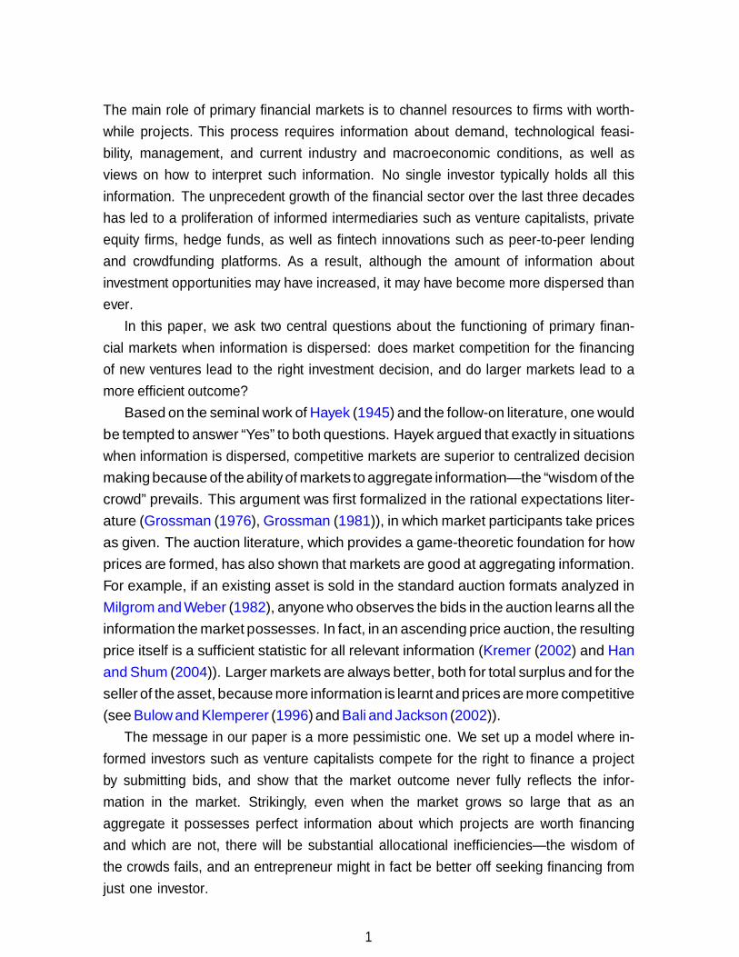
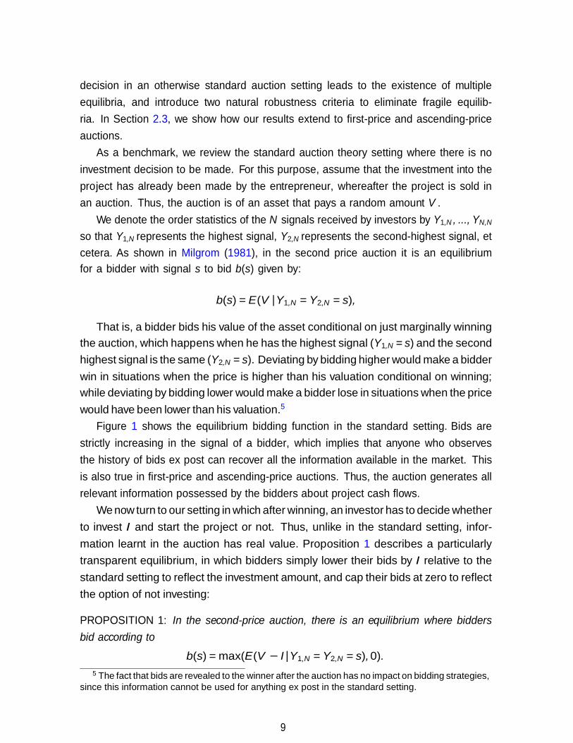
Figure 1 shows the equilibrium bidding function in the standard setting. Bids are strictly increasing in the signal of a bidder, which implies that anyone who observes the history of bids ex post can recover all the information available in the market. This is also true in first-price and ascending-price auctions. Thus, the auction generates all relevant information possessed by the bidders about project cash flows.

We now turn to our setting in which after winning, an investor has to decide whether to invest I and start the project or not. Thus, unlike in the standard setting, infor- mation learnt in the auction has real value. Proposition 1 describes a particularly transparent equilibrium, in which bidders simply lower their bids by I relative to the standard setting to reflect the investment amount, and cap their bids at zero to reflect the option of not investing:

PROPOSITION 1: In the second-price auction, there is an equilibrium where bidders bid according to

b(s) = max(E(V − I|Y1,N = Y2,N = s), 0).

5 The fact that bids are revealed to the winner after the auction has no impact on bidding strategies, since this information cannot be used for anything ex post in the standard setting.

9

Bidders with Si ≤ sN bid zero, where sN is defined as

sN = sup s : E(V − I|Y1,N = Y2,N = s)) ≤ 0. (2) The winner invests in the project if Y2,N > sN or if his own signal is sufficiently high, and otherwise does not invest.

We postpone the proof until Proposition 2, which considers a more general case.

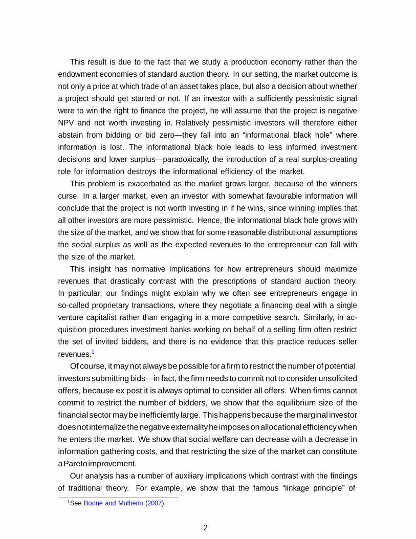
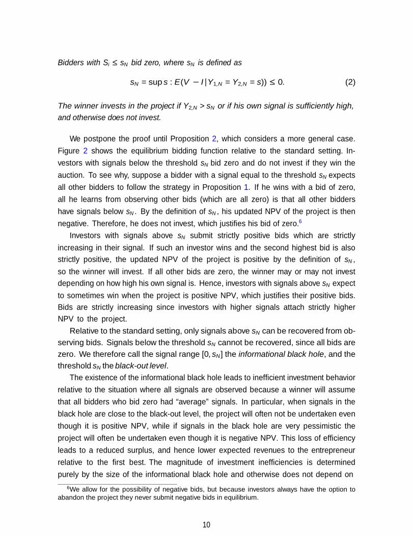
Figure 2 shows the equilibrium bidding function relative to the standard setting. In- vestors with signals below the threshold sN bid zero and do not invest if they win the auction. To see why, suppose a bidder with a signal equal to the threshold sN expects all other bidders to follow the strategy in Proposition 1. If he wins with a bid of zero, all he learns from observing other bids (which are all zero) is that all other bidders have signals below sN . By the definition of sN , his updated NPV of the project is then negative. Therefore, he does not invest, which justifies his bid of zero.6

Investors with signals above sN submit strictly positive bids which are strictly increasing in their signal. If such an investor wins and the second highest bid is also strictly positive, the updated NPV of the project is positive by the definition of sN , so the winner will invest. If all other bids are zero, the winner may or may not invest depending on how high his own signal is. Hence, investors with signals above sN expect to sometimes win when the project is positive NPV, which justifies their positive bids. Bids are strictly increasing since investors with higher signals attach strictly higher NPV to the project.

Relative to the standard setting, only signals above sN can be recovered from ob- serving bids. Signals below the threshold sN cannot be recovered, since all bids are zero. We therefore call the signal range [0, sN ] the informational black hole, and the threshold sN the black-out level.

The existence of the informational black hole leads to inefficient investment behavior relative to the situation where all signals are observed because a winner will assume that all bidders who bid zero had “average” signals. In particular, when signals in the black hole are close to the black-out level, the project will often not be undertaken even though it is positive NPV, while if signals in the black hole are very pessimistic the project will often be undertaken even though it is negative NPV. This loss of efficiency leads to a reduced surplus, and hence lower expected revenues to the entrepreneur relative to the first best. The magnitude of investment inefficiencies is determined purely by the size of the informational black hole and otherwise does not depend on

6We allow for the possibility of negative bids, but because investors always have the option to abandon the project they never submit negative bids in equilibrium.

10

i=1

the particular shape of the bidding function, as long as bids outside of the informational black hole are strictly increasing. We use this fact below to extent our results to other auction formats.

2.1. Strategic complementarities and multiple equilibria

Because the size of the informational black hole affects the efficiency of investment

decisions, there are strategic complementarities among investors. When an investor expects others to bid zero over a large signal interval so that the informational black hole is larger, he expects surplus from the auction to be lower because of the lost information, which justifies bidding lower and in particular bidding zero for higher signal realizations. Hence, the expectation of a larger informational black hole can be self-fulfilling. We next show that this feedback loop can lead to a continuum of equilibria characterized by different sizes of the informational black hole.

Proposition 2 establishes an upper and a lower bound on the equilibrium black-out level and shows that any black-out level in between can be supported in equilibrium:

PROPOSITION 2: Define the threshold sN as the highest signal such that

E[V − I|Y1,N =, . . . , = YN,N = sN ] ≤ 0, (3) and the threshold sN as the highest signal such that

E(V − I|Y1,N = sN ) ≤ 0. (4)

For any s ∈ [sN , sN ], there is a symmetric monotone equilibrium in the second-price

auction with black-out level s, in which a bidder with a signal s bids

b(s; s) = E [max (E[V − I|S>s], 0) |Y1,N = Y2,N = s] , (5) where S>s is the signal vector of investors censored below s:

S>s ≡ {max(Si, s)}N .

There is no symmetric monotone equilibrium with a black-out level outside this range.

Proof. The upper bound sN on feasible black-out levels is defined such that an investor who learns only that he has the top signal will invest if and only if his signal is above sN . To see why this is an upper bound, suppose to the contrary that there is an equilibrium in which a bidder with a signal slightly above sN is supposed to bid zero. If such a

11

bidder wins the auction, his updated NPV of the project is strictly positive from the definition of sN , so he makes strictly positive profits when winning. By an arbitrarily small increase of his bid, he is guaranteed to receive this profit without affecting the price he pays, a profitable deviation.

The lower bound sN on feasible black-out levels is defined such that the project just breaks even conditional on all investors having this signal. Suppose to the contrary that there is an equilibrium where a bidder with a signal s < sN bids a strictly positive amount. When such a bidder wins the auction in a monotone equilibrium, other bidders have signals weakly below his. By the definition of sN , the project is therefore always negative NPV when such a bidder wins, which is inconsistent with a strictly positive bid.

We next show that we can support any black-out level s ∈ [sN , sN ] in equilibrium. An investor who expects the black-out level to be s will assume that if he wins, he will be able to recover all signals above the black-out level when making his investment decision, which is equivalent to observing the censored vector of signals S>s defined in the proposition. Since a winner will invest only if the NPV is positive conditional on observing S>s, this is an auction of an option to invest which has random value max (E[V − I|S>s], 0). The equilibrium bidding function b(s; s) then takes the stan- dard form derived in Milgrom (1981): Investors bid their value of the project rights conditional on just marginally winning. The bidding function (5) will indeed constitute an equilibrium in our setting if it is consistent with the belief that the black-out level

is s, that is, if b(s; s) is zero for s ≤ s and is strictly positive and increasing for s > s. Notice that investors with signals below the black-out level s learn only that all signals are in the informational black hole when they win, which results in zero option value

of the project for any s ≤ sN . Therefore, it is optimal for them to bid zero. To prove that b(s; s) is strictly positive for s > s notice that if a bidder with signal above the the black-out level s ≥ sN wins the auction then there is a positive probability that all other bidders have their signals in the interval [sN , s], which results in positive option value, and therefore, a positive bid. The proof that b(s; s) is strictly increasing for s > s is the same as in Milgrom (1981). Q.E.D.

The feedback effect from the destruction of information to the value of the option to invest allows the black-out level to take any value in the range [sN , sN ]. The least efficient equilibrium is the one with the highest black-out level sN . In this equilibrium, only information in the highest signal affects the investment decision and no other information can be used. The equilibrium in Proposition 1 with black-out level sN

is more efficient because the top two signals can affect the investment decision. Fi- nally, the equilibrium with the lowest black-out level sN is the most efficient because

12

investment can be conditioned on the largest set of information.7 We next show that equilibria with black-out levels below sN are very fragile, so that the equilibrium in Proposition 1 is in fact the most efficient robust equilibrium.

2.2. Robust equilibria

In this section, we introduce two robustness criteria. The first one requires that an

equilibrium is a limit of equilibria in auctions where bids have to be made in increments of some δ > 0 as we let δ go to zero. Since all real-world markets have discrete price grids we view this as a natural requirement. We call such an equilibrium δ-bid robust.

Our second robustness criterion requires that an equilibrium is a limit of equilibria in auctions where bidders have to incur some cost ε > 0 for submitting a bid as we let ε go to zero. We allow bidders to not submit a bid to avoid this cost. We call such an equilibrium ε-cost robust.

The equilibria in the standard setting in all auction formats are both δ-bid and ε-cost robust. In our setting, Proposition 3 shows that the more efficient equilibria with black-out levels below sN are not δ-bid robust, and that equilibria with black-out levels below sN are not ε-cost robust.

PROPOSITION 3: There is no δ-bid robust symmetric monotone equilibrium in the second-price auction with black-out level below sN . There is no ε-cost robust symmetric monotone equilibrium in the second-price auction with black-out level below sN .

Proof. See the Appendix.

The formal proof is in the appendix. Here we provide a sketch of the proof. Consider an equilibrium with a black-out level s < sN , and an investor with a signal s very slightly above s who submits the minimal bid δ. If he wins the auction at price zero, so that all other bids are in the informational black hole, he concludes that the project is negative NPV and he does not invest. If he wins when only one other bidder bids δ, the updated NPV is also negative by the definition of sN . Hence, he loses the price δ. The only circumstance in which the investor can make profits from investing is when there are at least two other bidders who bid δ. But for small δ, as we show in the formal proof, the probability of tying at δ with more than one bidder becomes negligible relative to the loss event of tying with just one bidder. Hence the investor cannot break even with a non-zero bid, which contradicts that the black-out level is s < sN .

7Note that even this equilibrium has inefficiencies relative to the first best where all signals are observed because the black-out level sN is strictly positive.

13

Note that this argument does not extend to equilibria with black-out levels s ≥ sN

because by the definition of sN the project is positive NPV when a winner outside of the black hole ties with one other bidder. However, if bidders have to incur some arbitrarily small cost for submitting a bid (but can stay out of the auction for free), a parallel argument shows that the only viable equilibrium black-out level is the upper bound sN

even when bids do not need to be in discrete increments. To see this, consider again an investor very slightly above a candidate black-out level s < sN . From the definition of sN , such an investor can only make profits if at least one other bidder submits a lower but strictly positive bid. But the probability of this event becomes arbitrarily small for investors arbitrarily close to the black-out level, so that they cannot recoup the cost of submitting a bid. Therefore, the equilibrium unravels so that the only viable threshold is sN .

When we analyze how efficiency varies with the size of the market in Section 3, we will restrict attention to robust equilibria. Before turning to that analysis, we show how our results extend to other standard auction formats.

2.3. Ascending and First-Price Auctions

We now extend our results to the ascending-price and first-price auction formats.

The logic for the first-price auction is the same as for the second-price auction. Given a candidate black-out level s we can view our setting as an auction of an object with value

max (E[V − I|S>s], 0). This is the value of the option to do the project for someone who expects to observe all signals above the black-out level. In the first-price auction, the winner can infer all signals above the black-out level by observing bids ex post.

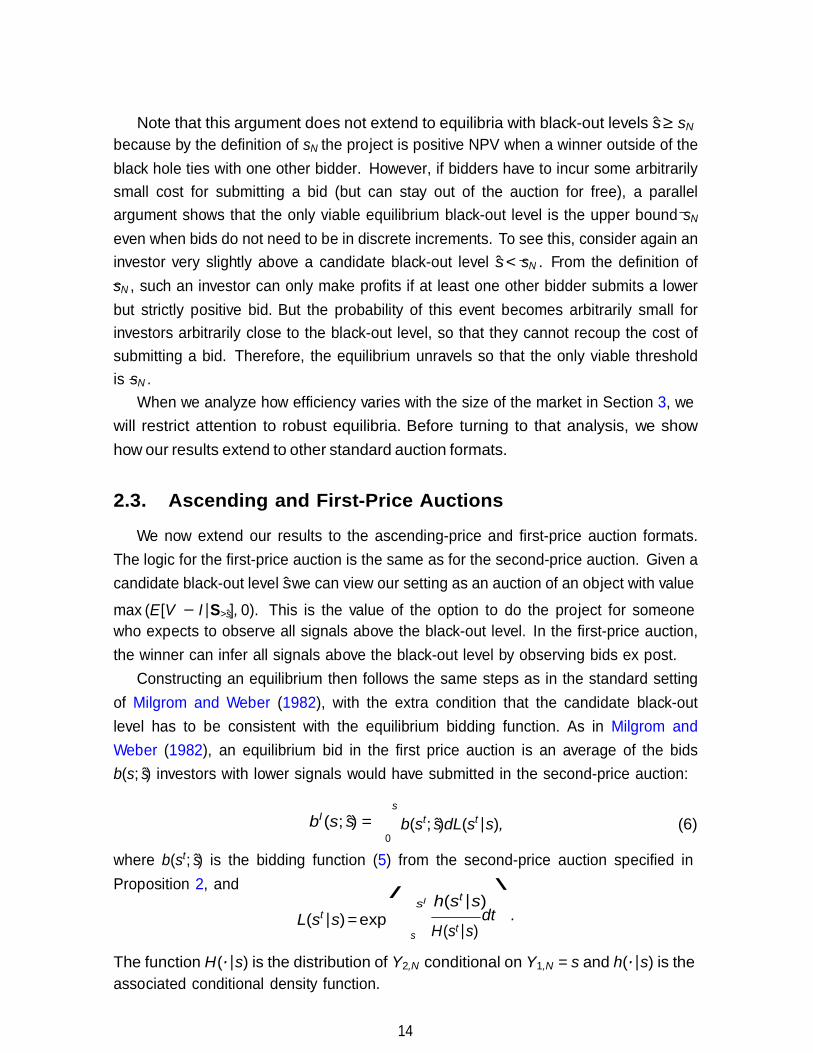
Constructing an equilibrium then follows the same steps as in the standard setting of Milgrom and Weber (1982), with the extra condition that the candidate black-out level has to be consistent with the equilibrium bidding function. As in Milgrom and Weber (1982), an equilibrium bid in the first price auction is an average of the bids b(s; s) investors with lower signals would have submitted in the second-price auction:

bI (s; s) =

s

b(st; s)dL(st|s), (6) 0

where b(st; s) is the bidding function (5) from the second-price auction specified in Proposition 2, and /

sl h(st|s) \

L(st|s) = exp dt .

s H(st|s)

The function H(·|s) is the distribution of Y2,N conditional on Y1,N = s and h(·|s) is the associated conditional density function.

14

Note that since b(st; s) is strictly positive if and only if st > s, the same is true for bI (s), so that the bidding function is consistent with the black-out level s. Following the same steps as the ones in the proof of Theorem 14 of Milgrom and Weber (1982) one can then show that bidding strategies bI (s; s) form an equilibrium in the first-price

auction for any black-out level s ∈ [sN , sN ]. The equilibria of the first-price auction turn out to be even more fragile than for

the second-price auction. This is because a winner has to pay his own bid, so that he incurs a loss whenever he does not invest. Following similar steps as for the second- price auction, one can show that only the equilibrium with the highest black-out level sN is δ-bid and ε-cost robust.8

Next consider the ascending-price auction. For black-out levels in the interval s ∈ [sN , sN ], exactly the same arguments as for the first-price and second-price auctions can be used to construct equilibria as in Milgrom and Weber (1982), where the object for sale has value max (E[V − I|S>s], 0). If the price goes above zero, which happens only if at least two bidders stay in, the project is always positive NPV from the definition of sN , so that the auction is completely standard.

However, for black-out levels below sN we have to take special care in defining how bidders can react when other bidders drop out as the price increases above zero. When multiple bidders drop out at price zero, other bidders who otherwise would stay in the auction may want to drop out immediately as well. Modelling this requires either that we allow players to condition their actions on the simultaneous actions of other players, or that bidders can drop out just as the price goes above zero. The first alternative is logically inconsistent, while the second is not well defined when price is increased continuously. For this reason we model price as increasing in discrete increments, and study equilibria in the limit as the size of the increments go to zero. Proposition 4 shows that the feasible equilibrium black-out levels are then exactly the same as the ones we derived for the robust second-price auctions in Proposition 3.

PROPOSITION 4: There is no δ-bid robust symmetric monotone equilibrium in the ascending-price auction with black-out level below sN . There is no ε-cost robust sym- metric monotone equilibrium in the ascending-price auction with black-out level below sN .

Proof. See the Appendix.

The argument that the black-out level cannot be below sN with discrete bids follows a similar logic as for the second-price auction. Suppose to the contrary that there is an

8The formal proof is in the online appendix.

15

equilibrium in which the black-out level is some signal s < sN , so that an investor with a signal just slightly above s stays in the auction until the price is slightly positive. This investor can win under three circumstances. First, he can win if all other bidders drop out at zero, in which case it is optimal not to start the project, which involves zero profits because the price is also zero. Second, he can win if only one other bidder stays in the auction and this bidder has a signal below sN , in which case it is also optimal not to start the project. Since the price is positive, this involves some losses. Third, he can win if more than two other bidders stays at positive prices, which could imply that the project is positive NPV. But in this scenario he only wins if other bidders have lower signals than him, a very small probability event. The expected profits will therefore be negative.

The argument for why an arbitrarily small cost ε of submitting a bid leads to the maximum black-out level is the same as for the second-price auction. For any candidate lower black-out level, an investor just above the threshold would be unable to recoup his cost because the probability of winning when the project is positive NPV is too small.

The results of this section and Section 2.2 above show that the most efficient black- out level in robust equilibria is either sN or sN , depending on what robustness criterion and what auction format we consider. The social surplus created is independent of the auction format and depends only on the black-out level. We now turn to the question of how surplus in robust equilibria changes with the size of the market.

3. Market size and informational efficiency

We now study the effect of market size on informational efficiency. We first show

that even as the market grows infinitely large so that aggregate information is perfect, substantial investment mistakes still occur. We then show that small markets can create both higher social surplus and higher entrepreneurial revenues than large markets. Finally, we endogenize the size of the market by assuming that investors have some cost of acquiring information and show that inefficiently large financial markets can occur in equilibrium.

3.1. Surplus in large markets

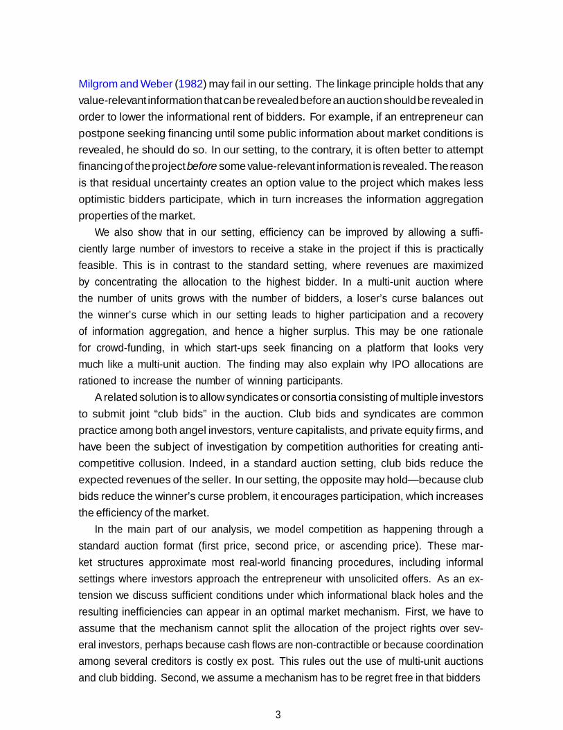
Figure 3 shows the effect of increasing the market size on bidding functions in our

setting relative to the standard setting. Panel A shows bidding functions for a smaller market and panel B for a larger market. In the standard setting, bids conditional on a

16

f f

given signal decrease with the number of bidders because the winner’s curse becomes stronger: Bidders condition on winning, and having the highest signal in a large sample is worse information than having the highest signal in a small sample. Nevertheless, all information is still recovered from observing bids, since the bidding function is strictly increasing. In the limit, as the market grows infinitely large, an observer of all bids in the standard setting will therefore learn the quality of the asset perfectly.

In our setting, as the market grows larger, the stronger winner’s curse leads to a larger informational black hole. Proposition 5 below shows that the informational black hole approaches the whole range of signals as N goes to infinity, and characterizes limiting investment behavior:

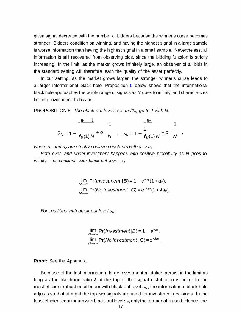
PROPOSITION 5: The black-out levels sN and sN go to 1 with N :

a1 1

1 a2

1

1

sN = 1 − B

+ o (1) N N , sN = 1 −

B + o ,

(1) N N

where a1 and a2 are strictly positive constants with a2 > a1. Both over- and under-investment happens with positive probability as N goes to

infinity. For equilibria with black-out level sN :

lim N →∞

lim N →∞

Pr(Investment |B) = 1 − e−a2 (1 + a2),

Pr(No Investment |G) = e−λa2 (1 + λa2).

For equilibria with black-out level sN :

lim N →∞

lim N →∞

Pr(Investment|B) = 1 − e−a1 ,

Pr(No Investment |G) = e−λa1 . Proof: See the Appendix.

Because of the lost information, large investment mistakes persist in the limit as long as the likelihood ratio λ at the top of the signal distribution is finite. In the most efficient robust equilibrium with black-out level sN , the informational black hole adjusts so that at most the top two signals are used for investment decisions. In the least efficient equilibrium with black-out level sN , only the top signal is used. Hence, the

17

first-best is never implemented unless top signals are infinitely informative. It is easy to verify that the least efficient equilibrium with black-out level sN has sizeably larger probability of both over- and under-investment than the most efficient equilibrium also in the limit.

3.2. Smaller versus larger markets

We next show that not only is the first best not achieved in the limit, but surplus

can actually go down as the market grows. Since investment depends entirely on the realization of either the highest or the second highest signal among bidders, increasing the market size is beneficial only if top signals become more informative as the “sample size” of signals grows.

PROPOSITION 6: If fG(s) / fB (s)

is a decreasing (increasing) function at s = 1 then

FG(s) FB (s) there is an N such that surplus decreases (increases) with N > N for equilibrium black-out levels sN and sN in all auction formats.

Proof: See the Appendix.

The ratio fG(s) / fB (s)

is a conditional likelihood ratio, which measures the informa- FG(s) FB (s)

tiveness of the top signal s if signals are restricted to be drawn from the interval [0, s]. If this ratio decreases with s, it means that not much of the information in the signal distribution is concentrated at the top end. Adding bidders then reduces efficiency, since it shifts the distribution of the pivotal order statistics Y1,N and Y2,N towards the less informative part of the distribution.

We now give three examples of signal distributions, one in which efficiency decreases with market size, one where it increases, and one where market size is irrelevant for efficiency.

Example 1: One example where the market becomes less efficient as the size increases is when information is coarse such that signals can take on only a finite number of discrete values. In our continuous representation, a discrete signal corresponds to an

interval (a, b] such that the likelihood ratio fG(s)/fB (s)) is flat for s ∈ (a, b]. At the top of the signal distribution, the likelihood ratio is then a constant λ over some interval (a, 1], so that

fG(s) / fB (s) FB (s) = λ , FG(s) FB (s) FG(s)

which decreases in s. Intuitively, the highest signal in a very large market will almost surely be in the highest interval regardless of the quality of the project. Hence, the realization of the top signal is not particularly informative. In a smaller market, on

18

the other hand, observing that the top signal is in the highest interval makes it more likely that the project is good rather than bad.

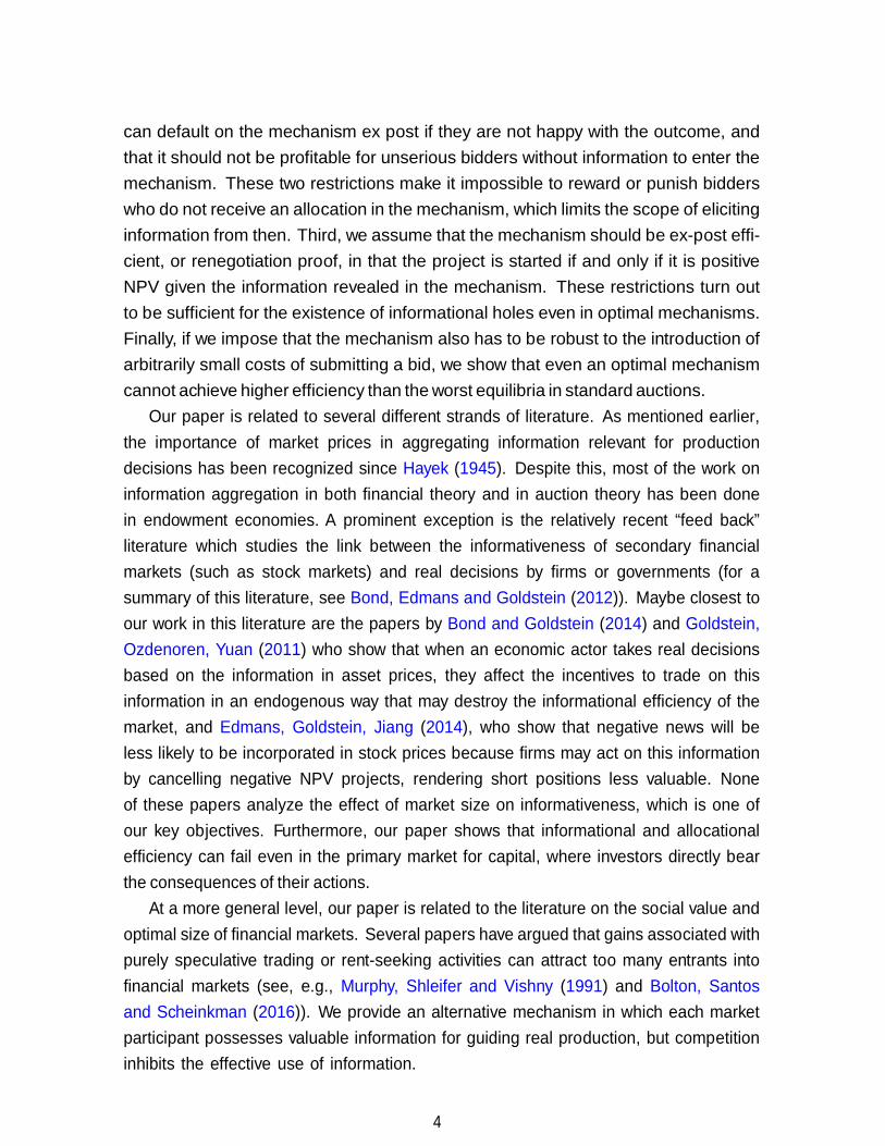
Figure 4 plots surplus as a function of the market size for binary signals. We assume that if the project is good, investors get only high signals, while if the project is bad, they are equally likely to get high and low signals. This binary signal structure can be

represented by setting fB (s) = 1 for all s ∈ [0, 1], and setting fG(s) = 0 for s ∈ [0, 1/2] and fG(s) = 2 for s > 1/2. We provide the full calculations for this example in the appendix.

In line with the results of Proposition 6 we can see in Figure 4 that in the least efficient equilibrium social surplus declines with the market size for all N —surplus is maximized with a single investor. In the most efficient robust equilibrium surplus is maximized with two investors and then declines with market size.

Example 2: Milgrom (1981) shows that a necessary and sufficient condition for the price in a second-price auction to converge to the true value of the asset as the number of bidders goes to infinity is that for any two values v and vt of the asset with vt > v,

f (s|v) inf

s f (s|vt) = 0,

where f (s|v) denotes the density of the signal distribution conditional on the value v. For example, this condition is satisfied if signals are normally distributed around the true value of the asset.9 In our setting, this condition can only hold if the likelihood ratio fG(s)/fB (s) goes to infinity at the top of the signal distribution. When this is the case, not only is surplus increasing in the size of the market, but all investment mistakes are eliminated in the limit. As Pesendorfer and Swinkels (1997) note, this condition is very strong—it requires that for any value v, there is a signal s such that an observer of that signal can rule out values below v.

Example 3: If fG(s) = asa−1 and fB (s) = bsb−1 with a > b, the ratio in Proposition 6 is constant, so the number of bidders is irrelevant for surplus.10

We next consider entrepreneurial revenues as a function of market size. If the entrepreneur has the power to pick the number of bidders, he will do so in order to maximize revenues rather than surplus. The private optimum may differ from the social optimum if the entrepreneur captures only part of the surplus. In our setting, the split of the surplus between the entrepreneur and investors has similar comparative

9The normal distribution has unbounded support, but can be represented on a unit interval by an appropriate change of variables.

10This specification is the exponential distribution transformed to a bounded support.

19

statics with respect to the number of bidders as in the standard auction theory setting of Milgrom and Weber (1982), where surplus itself is fixed. In particular, the fraction of surplus captured by the entrepreneur goes to one with N in all auction formats. Hence, if surplus increases with N , there is no conflict between the private and social optimum—the entrepreneur will prefer the maximal number of bidders.

The non-trivial case is when surplus decreases with N . Will the entrepreneur find it optimal to restrict the number of bidders even though this may entail surrendering a higher fraction of the surplus to investors? Our answer is a qualified “Yes”. The next proposition gives a sufficient condition for when this is the case.

PROPOSITION 7: Suppose that there exists an ε > 0 such that fG(s)/fB (s) = λ for s ∈ [1 − ε, 1] . Then, there exists some N such that revenue is strictly decreasing in N for N ≥ N .

Proof: We know that there exists some N such that sN ≥ 1 − ε for all N ≥ N . Over this interval, fG(s) / fB (s)

is strictly decreasing, and so from Proposition 6, surplus is FG(s) FB (s)

decreasing in N for N > N . All bidders must make the same expected profits since they are in the same equivalence interval. Since some bidders do not participate, the expected bidder profits are zero, and hence revenues coincide with surplus. Q.E.D.

To understand this result, note that surplus decreases with N when the top of the

signal distribution is relatively flat, so that investors who draw high signals are infor- mationally close to each other. But when this is the case, investors also capture little informational rent even for moderate levels of N . In other words, increasing N beyond a certain level has little effect on the split of revenues but a large negative effect on sur- plus. As an illustration, in the example of Figure 4 where investors get binary signals, bidders earn exactly zero surplus whenever N > 1 because of competition between informationally identical bidders from the top equivalence interval. Hence, whenever surplus is maximized at some market size N > 1, the social optimum coincides with the entrepreneur’s private optimum. For the least efficient equilibrium, the social optimum is to have one investor. For this case the entrepreneur may prefer inviting an extra bidder despite the loss of surplus in order to increase competition.11

The conditions in Proposition 7 are sufficient but not necessary for the entrepreneur to prefer a smaller market. As Example 4 in the next section shows, the entrepreneur will prefer a smaller market whenever the likelihood ratio does not increase too steeply at the top of the signal distribution.

11Even for N = 1, the entrepreneur can capture the full surplus if he has enough commitment power to set an appropriate reserve price.

20

Our results provide one explanation for why so many capital raising situations involve negotiations with a restricted set of investors rather than an auction open to everyone.

3.3. Can financial markets be too big?

In the previous section we established that small markets may be preferable both

from the entrepreneur’s and from a social surplus perspective. In this section we show that the equilibrium size of the market can be too large relative to both the social and the entrepreneurial optimum, and can be Pareto inferior relative to a market with one less investor.

If the entrepreneur can commit to seek financing from a restricted set of investors, the market can obviously never be larger than what is optimal for the entrepreneur. However, restricting the set of potential investors may be difficult in practice because it is ex post optimal for the entrepreneur to consider any offer he receives, even if the offer is unsolicited. In this section we therefore assume no commitment so that investors can enter any auction.

So far, we have assumed that investors observe signals for free to make our results on the failure of information aggregation in large markets as striking as possible. In order to have a non-trivial equilibrium market size, we now assume that investors face some costs of gathering information.

Assume that each potential investors i has a cost ci of gathering information about the project, and that ci is strictly increasing. We focus on the case where fG(s) / fB (s)

FG(s) FB (s)

is a decreasing function around s = 1 so that social surplus (gross of investor costs) is maximized at a finite market size. The socially optimal market size net of costs is then even smaller.

We also assume that MLRP holds strictly, which ensures that investors have strictly positive expected profits from participating in the market gross of their information gathering cost. We then have the following result:

PROPOSITION 8: Suppose that fG(s) / fB (s)

is a decreasing function around s = 1

FG(s) FB (s) and that MLRP holds strictly. Then, there is a c > 0 such that if sufficiently many investors have costs of gathering information below c, the equilibrium size of the market is larger than the socially optimal size. Lowering information gathering costs can lead to a decrease in social surplus.

Proof: See the Appendix.

The proposition shows that there is no reason to believe that markets will become

21

more efficient as information technology improves. This is in contrast to the predictions of Samuelson (1985) and Levin and Smith (1994) who study information costs in an otherwise standard auction theory setting. In both papers, the optimal size of the market goes to infinity as costs go to zero.

Proposition 8 shows that there can be too much entry in equilibrium relative to the social optimum. The next example shows that both investors and the entrepreneur can be better off if entry is restricted.

Example 4: Suppose that fB (s) ≡ 1 and fG(s) is a truncation to the interval [0, 1] of

a normal distribution with mean 1 and standard deviation 0.75. The likelihood ratio fG(s)/fB (s) is strictly increasing over [0, 1], so MLRP holds strictly. Also, because the derivative of the likelihood ratio is zero at s = 1, the ratio fG(s) / fB (s)

is a decreasing FG(s) FB (s)

function around s = 1. We assume that the net present value for a good project is 0.75, while a bad project has an NPV of minus one.

Panel A of Figure 5 shows social surplus gross of investor costs and the expected revenues to the entrepreneur as a function of the size of the market. The figure is drawn for the most efficient robust equilibrium where the black-out level is sN . Social surplus is maximized at a market size of three, while the entrepreneur’s revenues are maximized at a market size of four. The entrepreneur prefers a somewhat larger market size than what maximizes social surplus because increased competition between investors reduces their share of the surplus.

Panel B shows expected gross profits to investors from participating in the auction as a function of market size, as well as a particular specification for the cost ci of information gathering for each investor. In equilibrium, investors will enter as long as expected profits cover their cost, so that for the specific costs drawn in the figure the first 10 investors will enter in equilibrium with investor 10 indifferent between entering and staying out. Hence, the equilibrium market size is larger than both the social optimum and the entrepreneur’s optimum.

Now suppose that every investor’s cost was just slightly larger. This would be the case if, for example, tax rates on venture capitalist profits are increased slightly. The equilibrium market size would drop to 9, which would constitute a Pareto improvement. Participating investors would make higher profits because of both reduced competition and more efficient investment decisions. The entrepreneur’s revenues would increase because the increased surplus from more efficient investment outweighs the loss from reduced competition. Finally, the investor who drops out of the market is no worse off since he was just breaking even before.

22

4. Strategies for reducing the winner’s curse

The source of inefficiency in our model is the effect the winner’s curse has on the participation of pessimistic bidders, an effect that becomes stronger as the market grows larger. In this section we discuss a number of strategies that can help to alleviate the winner’s curse. First, we show that it may be beneficial to raise capital before important information is learnt in order to increase the option value embedded in the project. Second, we show that allowing a larger set of investors to co-finance the project helps reduce the winner’s curse. Third, in contrast to results for standard auctions, we show that allowing bidders to collude ex ante via bidding clubs can also improve efficiency and revenues. Finally, we discuss how adding an appropriately designed derivative market where investors can bet on project failures might eliminate the informational black hole. All these “fixes” rely on alternative trading mechanisms that may not always be implementable in practice. In Section 5 we provide a systematic treatment of the conditions that lead to informational black holes in optimal mechanisms.

4.1. Choosing when to finance and the linkage principle

Suppose that there is some exogenous signal affiliated with the value of the project

that gets realized either before or after the auction. For example, this could be a signal about demand conditions for the products the project is meant to create, or any information the entrepreneur might have about the project that can be credibly communicated to the bidders. The question we ask is whether it is better to run the auction before or after this information is released.

For standard auctions, where no action is taken, the linkage principle of Milgrom and Weber (1982) suggests that it is better to run the auction after all value-relevant information is realized in order to lower the informational asymmetry between bidders. However, in our setting we have an extra effect: If the signal is revealed after the auction but before the investment decision is made, the project has some real option value when bids are submitted, and so even bidders with low signals might want to participate. This could break the destruction of information.

We now give an example where the linkage principle fails in our setting. Suppose that a public signal SP ∈ {sG, sB } will be released at date t, where Pr(SP = sG|B) = 0 and Pr(SP = sG|G) = q, q ∈ (0, 1). Hence, when the public signal is sG, the project NPV is positive regardless of the bidders’ signals.

Suppose first that the entrepreneur runs the auction after the public information is released, as the linkage principle prescribes. We now calculate the expected surplus

23

Pr(G)(1−q)

generated by the auction. With probability q Pr(G) the public signal reveals that the project is good, so surplus is E(V − I|G). With probability (1 − q) Pr(G) + 1 − Pr(G), the public signal is sB and the updated prior on the project being good is Pr(G|sB ) =

Pr(G)(1−q)+(1−Pr(G)) < Pr(G), in which case the auction generates some surplus W , which from Proposition 6 is strictly below the first-best surplus. The expected surplus is then

q Pr(G)E(V − I|G) + ((1 − q) Pr(G) + 1 − Pr(G))W < Pr(G)E(V − I|G).

Suppose to the contrary that the entrepreneur runs the auction before the public signal is released, and that winners can wait to observe the public signal before they make the decision to start the project. In this case, everyone participates in the auction and there is no informational black hole. To see this, notice that even for the most pessimistic bidders, the option to do the project has some strictly positive value since there is always some strictly positive probability that the public signal will reveal the project to be good. It is then easy to verify that bids will be strictly positive and strictly increasing in signals for all N . As a result, all informational properties of the auction are the same as in the standard setting. In particular, ascending-price auctions aggregate all information and leads to first-best investment decisions when the market grows large, and the same holds for first-price and second-price auction if bids are revealed ex post. Furthermore, the expected revenue converges to the expected surplus as N goes to infinity. Hence, the seller is better off running the auction before the public signal is revealed.

Remark 1: Our exercise in this section compares the effect of running the auction before or after some public release of information, rather than asking whether releasing information is better than never releasing it at all. In the standard model of Milgrom and Weber (1982) this distinction is irrelevant, since ex post releases of information have no impact on the expected value of the asset up for sale. If the choice is whether to release information before the auction or never, Theorem 18 of Milgrom and Weber (1982) can be applied to show that the linkage principle holds for the least efficient equilibria. Whether this version of the linkage principle holds for our wider set of equilibria is an open question.

Remark 2: The results in this section show that if the decision to start the project can be postponed indefinitely and costlessly, and if there is any possibility that the project can become positive net present value sometime in the future even for the most pessimistic investors, then the informational black hole will be eliminated and the auction will properly aggregate information (assuming bids are revealed ex post). Hence an important underlying assumption for our results is that the option to start the

24

project has some natural expiration date, or that there are sufficient costs associated with keeping the option alive. We believe this to be a natural assumption for most real options.

4.2. Dispersed ownership

In the previous sections we assumed that only one investor ends up with a stake

in the project. In this section we allow for the possibility that K > 1 investors can co-finance the project. Allowing for more investors to receive an allocation weakens the winner’s curse and hence encourages more investors to submit non-zero bids, which has a positive effect on efficiency. Pesendorfer and Swinkels (1997) show that the K- unit auction has a unique symmetric monotone equilibrium in the standard setting and

that the auction fully aggregates information as N → ∞ if and only if K satisfies the “double largeness” condition: K → ∞ and N − K → ∞.

While there are multiple equilibria in our setting, we show that the aggregation properties of K-unit auction mirror those of Pesendorfer and Swinkels (1997). In particular, inefficiencies persist as long as K is finite, even if the bids are made known after the auction and are incorporated in the investment decision. The case of finite K seems reasonable in most corporate finance situations. If K is allowed to grow proportionately with N , we show that inefficiencies disappear in the limit.

Specifically, we assume that the K highest bidders who submit nonzero bids share the investment costs and the project’s payoff. Each bidder pays the bid submitted by the K + 1st highest bidder. If there are less than K bidders who submit nonzero bids the project is cancelled. Otherwise the K highest bidders get the right to finance the project. In principle, winning bidders may disagree about the decision to start the project. When K grows with N we show that for large N all winning bidders agree on the investment decision. When K is finite we consider the optimistic scenario in which all winning investors share their information with each other and jointly decide whether to start the project.

PROPOSITION 9: In the K-unit auction, for any finite K, the limiting surplus is strictly lower than the first-best expected surplus. If K/N goes to some constant larger than zero and smaller than one, then the expected surplus converges to the first-best expected surplus.

Proof: See the Appendix.

Our results in this section can be used to explain why firms explicitly ration the

allocation of shares in initial public offerings so that a larger number of investors receive

25

an allocation. It can also explain why entrepreneurs often allow a number of venture capitalists to co-invest, and the increasing popularity of crowd-funding platforms.

Remark 3: Atakan and Ekmekci (2014) study K-unit auctions in which double- largeness holds and in which information is not fully aggregated in the limit. Their equilibria are specific to the multi-unit setting and fail to exist in a single-unit setting. Our results are the reverse—information is aggregated when double-largeness holds but not when K is finite. In this sense, our papers are complementary.

4.3. Syndicates and club bids

We now study a setting in which bidders can form consortia and submit a joint

bid. We provide an example in which allowing such “club bids” has a positive effect on surplus and revenues. This is in contrast to the intuition from the standard setting, where collusion among bidders tends to lower seller revenues.

A full analysis of club bidding is challenging for several reasons. First, club forma- tion is an endogenous process which may lead to clubs of different size, which would require analysis of auctions with asymmetric bidders. Second, there may be incentive problems within the club that prevent full sharing of information among club members. Third, even if information is freely shared within the club, the resulting information is multidimensional, which makes analysis of the resulting auction technically challenging.

Dealing with these issues is beyond the scope of our paper and we therefore consider a simplified setting where we assume clubs are of equal and exogenously given size, and that information is freely shared within the club. We also assume that individual signals are distributed as in Proposition 7 and that the market is sufficiently large, which as we explain below makes it possible to handle multidimensional signals in a straightforward way.

We assume that there are N × M investors in the market. We will contrast two market settings. In the first, there is no collusion among bidders and everyone submits bids independently. In the second, investors are randomly allocated to N symmetric clubs each consisting of M investors, whereupon each club submits a joint bid in the auction. Our question is whether an auction with club bids generates more revenue than a non-collusive auction.

As a benchmark, we first consider the standard auction setting where the asset for sale is already in place. In this setting, surplus is always the same. Under the assumptions of Proposition 7, the results in Axelson (2008) imply that in the first- price and second-price auctions, larger clubs lead to lower revenues when the number of participants is large.

26

In our investment setting, suppose we hold the number of club members M fixed and let the number of clubs N grow large. Recall that Proposition 7 assumes that individual signals have a constant likelihood ratio λ = fG(s)/fB (s) over some interval at the top of the signal distribution, which is a sufficient condition for the entrepreneur to prefer smaller markets. If the number of clubs N is large enough, only clubs where all members have signals in the top interval will participate because of the winner’s curse. The likelihood ratio corresponding to a situation where M members have signals in the top interval is then λM . Since λ > 1, this likelihood ratio increases in the size of the club—in other words, the fact that all members in a club are optimistic is a stronger signal the more members there are.

We show in the proof of Proposition 6 that the asymptotic surplus is an increasing function of the likelihood ratio at the top of the signal distribution, which is a natural consequence of the fact that a signal with a higher likelihood ratio is more informative and leads to smaller investment mistakes. It then follows immediately that for a large enough market larger clubs lead to higher social surplus. Furthermore, we show in the proof of Proposition 7 that all this surplus goes to the entrepreneur, and hence the entrepreneur is better off with club bidding.

There are two forces favoring club bidding in our setting. First, club bidding reduces the effective number of bidders, which is beneficial when markets are inefficiently large, even if the club would submit a bid based on the signal of only one member. Second, signals become more informative whenever there is some information sharing within the club. When these effects outweigh the reduced competition, the entrepreneur gains. Our theory provides a benign rationale for the prevalent use of club bids in private equity and the use of syndicates in venture capital that has come under scrutiny by competition authorities.12

4.4. Shorting markets

The informational black hole appears because pessimistic investors have no incentive

to bid in the auction. It could therefore be in the interest of the entrepreneur to create a market which rewards pessimistic bidders for expressing their views, in a similar way that short sellers in equity markets can profit on their information when they think a stock is overvalued. We now discuss how creation of such a market can remove the informational black hole.

There are at least three problems in constructing such a market. First, a derivatives market in which investors can take zero-sum bets would not be possible because there

12See Bailey (2007) for further discussion.

27

are no gains from trade due to the pure common value nature of the project, and so the no-trade theorem applies. As a result, any side market would have to be subsidized and would not appear spontaneously.

Second, one has to be careful in the design of the contract to avoid further informa- tional black holes to appear. For example, a contract which is short the cash flows of the project relies on the project actually being started, and so would not be attractive to the most pessimistic bidders. Similarly, a bet on whether the project is started or not would have a black hole where only the most pessimistic bidders participate. Fi- nally, a side market can lead to negative externalities on the original financing market due to strategic interactions.

Addressing all these issues rigorously goes beyond the scope of the current paper. Here we just conjecture a design that may reduce or eliminate the informational black hole. For example, suppose the entrepreneur subsidizes a side market and sells a contract which promises to pay $1 if the project is not started, or if the project is started but fails, and pays $0 if the project is started and succeeds. The entrepreneur then sells the project rights and the shorting contract in two independent, simultaneous auctions, whereafter all bids are revealed so that information from the shorting market can be used when making the investment decision. We conjecture that in a sufficiently large market, bids in the shorting market will be strictly decreasing in bidder signals, and hence observing the bids in the shorting market is equivalent to observing all signals. This would eliminate the informational black hole in the original market and lead to a first-best solution.

5. When do informational black holes exist in op-

timal mechanisms?

The previous section illustrates a number of special examples of augmented selling procedures that eliminate the informational black hole. In fact, it is well-know that in a pure common value setting such as ours, there are mechanisms that can fully extract the information of bidders at virtually no cost for the entrepreneur if no restrictions are put on allowable mechanisms (see for example McAfee, McMillan and Reny (1989)). These mechanisms have been criticized for their sometimes esoteric structure and for their lack of “robustness” to small changes in the environment, which is one of the reasons that our main focus in this paper is on the tried and tested standard auction procedures. Nonetheless, it is natural to ask what type of robustness criteria are needed for our results to go through in a mechanism design setting where general selling mechanisms

28

are allowed. We show two results. First, we develop a set of robustness criteria under which

any direct mechanism in which bidders either report their true signal or nothing has equilibria with informational black holes. In other words, an equilibrium without an in- formational black hole cannot be uniquely implemented in direct mechanism.13 Second, we show that if we also require mechanisms to be ε-cost robust, an optimal mechanism cannot improve on the least efficient equilibria with black-out level sN .

Consider a direct mechanism in which bidders either report their true signal or nothing (which we denote by a report of ∅). We denote a set of reports by R =

{r1, ..., rN }. A mechanism is a function Q(R) = {q1(R), ..., qN (R)}, which for each set of reports R assigns probability qi(R) that bidder i gets allocated the project rights, an outcome A(R) ∈ {0, 1, ..., N } of the lottery Q(R), where A(R) is the winning bidder (A(R) = 0 is the situation where the seller keeps the project rights), and a set of transfers t(R, A(R)) = {t1(R, A(R)), ..., tN (R, A(R))} from bidders to the seller (which

could be negative, if bidders are paid by the seller). A bidder who gets allocated the project rights and does not walk away from the mechanism gets the net project payoff

E(V − I|R) if the project is started. The first robustness condition we impose rules out mechanisms that split the allo-

cation over several bidders, such as a K-unit auction or collusion among bidders.

Condition 1: (Winner-take-all) The project is indivisible, with non-contractible cash flows, and the mechanism must allocate the project to the highest-signal investor or no one at all if no signals are reported.

Notice that it is not enough to require that the project can only be allocated to one bidder, because the equilibrium of the K-unit auction can be implemented by allocating the entire project to one of the K highest bidders through a lottery, rather than splitting the allocation over many bidders. Hence, we require that the mechanism is such that it allocates the project to the highest signal bidder.

There are two possible ways to justify this condition: First, if the highest signal bidder also has some small private value component which is higher than other bidders (such as lower costs or better skills in running the project), it is ex post efficient to allocate the project to him, and the highest-signal bidder would be allocated the project in a renegotiation proof mechanism. Second, the highest signal bidder will also have the highest ex post willingness to pay, so a seller without sufficient commitment power may be tempted to allocate the full project rights to him. The next two conditions put restrictions on the type of admissible transfers.

13Whether such an equilibrium can be uniquely implemented in an indirect mechanism remains an open question.

29

Condition 2: (Fly-by-night free) No bidder without private information can strictly profit from entering the mechanism.

Condition 3: (Regret free) No bidder would prefer ex post to exit the mechanism.

Condition 2 ensures that the mechanism is not swamped by unserious “fly-by-night” operators masquerading as serious bidders but without private information. If there is an infinite supply of such fly-by-night operators, a mechanism that rewards them for revealing their “signal” would quickly run out of money.14 Imposing this condition ensures that losers in the auction never get any positive transfers. Condition 3 ensures that losers never pay.15 The combination of conditions 2 and 3 makes it impossible to give bidders a strict incentive to reveal their information if they expect to never implement the project if they win the auction. Finally, we require that the mechanism is renegotiation proof in the following sense:

Condition 4: (Renegotiation proof ) The project is implemented if and only if it is positive NPV conditional on the information revealed in the mechanism.

If the mechanism is not required to be renegotiation proof, an entrepreneur with per- sonal wealth could eliminate the informational black hole by promising to fund the project with some small probability independent of bids. This would give all bidders an incentive to bid something strictly positive, and bids would be strictly increasing in signals.

We show in Proposition 10 that conditions 1-4 are sufficient for informational black holes to exist as the outcome in any mechanism. If we also assume that equilibria have to be ε-cost robust, that is, robust to introducing an arbitrarily small cost for bidders to reveal their signal, we show that any equilibrium must contain a black hole of the maximal size.

PROPOSITION 10: Under conditions 1-4, it is incentive compatible in any direct mechanism for bidders not to reveal their signal below the black-out level sN . Under conditions 1-4, an optimal ε-cost robust equilibrium has black-out level sN .

Proof: See the Appendix.

14See Rajan (1992) and Axelson, Stromberg, and Weibach (2009) for related robustness criteria. 15See Lopomo (2000) and Bergemann and Morris (2005) for related robustness criteria.

30

6. Other robustness issues 6.1. Security auctions

We first show that all our results remain true in the case of security auctions, in

which investors finance the project in exchange for part of the profits. Suppose the project’s payoff in our setting is either 0 or 1 + X. Then, a security auction takes

a particularly simple form: bidders submit interest rates Ri ∈ [0, X] at which they are willing to finance the project. The auction proceeds in the same way as for cash auctions, except that the winner is the bidder submitting the lowest interest rate.

We assume that the decision to start the project rests with the entrepreneur unless the winning bid is X, in which case the entrepreneur gives up all the cash flow rights, and therefore control rights are transferred to the winning bidder.

Notice that whenever the winning bid is below X the entrepreneur always starts the project. Hence, a bidder who submits a bid below X should be prepared to finance and start the project if he wins the auction. Hence, the black-out region in the first-price security auction is exactly the same as the one in the first-price cash auction.

In the second-price and ascending-price security auctions, a winner who gets to finance the project at the interest rate X has an option not to start it even if his own winning bid is below X. This is the same option that a winner in the cash option has when the latter wins and pays 0. Thus, there is one-to-one map between the size of the informational black hole in the second-price and ascending-price security and cash auctions.

Because social surplus depends solely on the size of the informational black hole, social surplus is the same in the security auction as in the cash auction.

6.2. Assets in place and entrepreneurial wealth

We have assumed that the entrepreneur has no wealth of his own to finance the

project, and no other assets that can be pledged to investors in exchange for financing. The model easily extends to the case of an existing firm raising financing for a new project, where the firm could either use some of its cash to co-finance the project or issue securities that are backed not only by the cash flows of the new project but also by the existing assets of the firm.

First, imagine that the entrepreneur has some wealth w, and issues an equity stake backed by a fraction 1 − w of the cash-flows of the project, where the winner invests 1 − w and the entrepreneur invests w to start the project if they find it optimal to

do so. It is easy to see that this leads to the exact same equilibria as when there is

31

no wealth, except that all prices and bids are scaled down by a factor 1 − w. Hence, surplus is exactly the same independent of the wealth of the entrepreneur. The only change is that revenues of the entrepreneur go up with wealth, since the fraction of

surplus captured by investors goes down by a factor 1 − w. This effect reinforces our result in Proposition 7 that revenues can go down with the number of bidders: as w goes to one, revenues will behave in exactly the same way as surplus.

One can also show that the entrepreneur would never want to subsidize investors by giving up a larger share of the project than 1 − w. Doing so would lower equilibrium

black-out levels, but only because investors sometimes would find it optimal to pursue negative NPV projects, which would lead to a destruction of surplus.

Now suppose that the entrepreneur does not have liquid wealth, but has an existing firm with assets that can be pledged to back the security issue. For example, suppose the firm has assets in place with random but positive cash flows Z uncorrelated with the project’s cash flows and that the firm issues new shares backed by both the assets in place and the new project. Suppose the firm runs a security auction in which investors bid the fraction of shares α they are willing to accept in exchange for the capital needed to finance the project. The most pessimistic investors would then submit a bid of 1/E(Z + 1); this is the fraction of shares needed to break even on an investment of 1 if the project is not pursued and the money raised is kept within the firm. The equilibrium black-out level below which investors submit this bid would be exactly the same as in our original model, so surplus would also remain the same. Again, as in the case of wealth, the entrepreneur would capture a larger share of the surplus the larger the value of the existing assets are, but investment efficiency would not be improved.

7. Conclusion

Our paper studies information aggregation in primary financial markets. We show

that information aggregation is severely impeded once information has real value for guiding investment decisions, and that the inefficiencies grow larger with the size of the market. Our analysis shows that several intuitive prescriptions from standard theory need to be reexamined when information has a real allocational role: a more competitive, larger financial market is not always better, early releases of information may be suboptimal, and collusion among investors may be beneficial for an entrepreneur seeking financing.

32

References Atakan, A.E., and M. Ekmekci, (2014) “Auctions, actions, and the failure of informa-

tion aggregation”, American Economic Review, vol. 104, 2014-2048. Axelson, U., (2008) “Bundling, rationing, and dispersion strategies in private and

common value auctions,” working paper, London School of Economics. Axelson, U., and I. Makarov (2016), “Sequential credit markets,” working paper, Lon-

don School of Economics. Axelson, U., Stromberg P., and M. S. Weisbach, (2009) “Why Are Buyouts Levered?

The Financial Structure of Private Equity Funds”, Journal of Finance, vol. 64, 1549– 1582.

Bailey, E. (2007), “Are private equity consortia anticompetitive? The economics of

club bidding,” The Antitrust Source 6(4), 18. Bali, V., and M. Jackson (2002), “Asymptotic revenue equivalence in auctions,” Journal

of Economic Theory, vol. 106, 161-176. Bergemann, D., and S. Morris, (2005) “Robust Mechanism Design”, Econometrica, vol.

73, 1771-1813.

Board, S., (2007) “Selling options”, Journal of Economic Theory, vol. 136, 324-340.

Bolton, P., T. Santos, and J. A. Scheinkman, 2016, “Cream Skimming in Financial Markets,” forthcoming, Journal of Finance.

Bond, P., Edmans, A., and I. Goldstein, (2012) “The real effects of financial markets”,

Annual Review of Financial EconomicsJournal, vol. 2012:4, 339-360. Bond, P., and I. Goldstein, (2014) “Government intervention and information aggre-

gation by prices”, forthcoming, Journal of Finance. Boone, A. L., and J. H. Mulherin, (2007) “How are firms sold?”, Journal of Finance,

vol. 62, 847-875. Broecker, T., (1990) “Credit-worthiness tests and interbank competition”, Economet-

rica, vol. 58, 429-452. Bulow, J., and P. Klemperer, (2002) “Prices and the Winner’s Curse”, RAND Journal

of Economics, vol. 33, 1-21.

33

Bulow, J., and P. Klemperer, (1996) “Auctions vs. negotiations”, American Economic Review, vol. 86, 180-194.

Cong, L.W., (2014) “Auctions of real options”, working paper, Stanford University.

Edmans, A., Goldstein, I., and W. Jiang, (2014) “Feedback effects, asymmetric trading,

and the limits to arbitrage,” working paper, London Business School. Embrechts, P., Kluppelberg C. and T. Mikosch, (2012), Modelling Extremal Events for

Insurance and Finance (Springer). Gertner, R., and D. Scharfstein, (1991) “A theory of workouts and the effects of reor-

ganization law,” Journal of Finance Vol. 46, 1189-1222. Goldstein, I., Ozdenoren, E., and K. Yuan (2011), “Learning and complementarities in

speculative attacks,” Review of Economic Studies 78, 263–292. Grossman, S.J. (1976), “On the efficiency of competitive stock markets where trades

have diverse information,” Journal of Finance 31, 573–585. Grossman, S.J. (1981), “An introduction to the theory of rational expectations under

asymmetric information,” Review of Economic Studies 48, 541–559. Grossman, S.J., and O. Hart (1980) “Takeover bids, the free-rider problem, and the

theory of the corporation,” Bell Journal of Economics Vol. 11, 42–64. Han, H., and M. Shum (2004), “Rates of information aggregation in common value

auctions,” Journal of Economic Theory 116, 1–40. Hayek, F. (1945), “The Use of Knowledge in Society,” American Economic Review 35,

519-530. Ilan Kremer (2002). “Information aggregation in common value auctions,” Economet-

rica, vol. 70(4), 1675-1682. Levin D., and J. L. Smith (1994), “Equilibrium in Auctions with Entry”, American

Economic Review 84, pp. 585-599. Lopomo, G. (2000), “Optimality and robustness of the English auction,” Games and

Economic Behavior 36, 219–240. McAfee, R. P., McMillan, J., and P. J. Reny (1989), “Extracting the surplus in the

common-value auction,” Econometrica 57, 1451-1459.

34

Milgrom, Paul (1981), “Rational expectations, information acquisition, and competi- tive bidding,” Econometrica, vol. 49, 921-943.

Milgrom, P. and R. Weber (1982). “A Theory of Auctions and Competitive Bidding,”

Econometrica, vol. 50, 1089-1122. Murphy, K. M., A. Shleifer and R. W. Vishny, 1991, “The Allocation of Talent: Impli-

cations for Growth,” Quarterly Journal of Economics 106, 503–530. Myers, S. C. (1977), “Determinants of corporate borrowing,” Journal of Financial

Economics 5, 147-175. Pesendorfer W. and J. Swinkels (1997). “The Loser’s Curse and Information Aggrega-

tion in Common Value Auctions,” Econometrica, vol. 65, 1247-1283. Rajan, R., (1992) “Insiders and Outsiders: The Choice between Informed and Arm’s-

Length Debt”, Journal of Finance, vol. 47, 1367–1400. Samuelson, W. F. (1985), “Competitive Bidding with Entry Costs.” Economics Letters

17, pp. 53-57. Shleifer, A., and R. W. Vishny (1986), “Large shareholders and corporate control,”

Journal of Political Economy 94, 461-488.

35

N

Appendix. Proofs Proof of Proposition 3: For convenience, the proof assumes that fG(s) and fB (s) are continuous. The proof extends to the case with jump points.

Part 1. First, we show that there is no δ-bid robust symmetric monotone equi- librium in the second-price auction with black-out level below sN . Suppose to the contrary that there exists such an equilibrium. It must then be the case that for any d > 0, we can find a δ ∈ (0, d] such that if bids have to be made in increments of δ, there is an equilibrium black-out level below sN . Let s < sN be a candidate black-out level such that it is the largest signal at which the zero bid is submitted. Let ∆1 be such that investors with signals in the interval (s, s + ∆1] bid δ, and ∆2 be such that investors with signals in the interval (s + ∆1, s + ∆1 + ∆2] bid 2δ.16 We assume that s is such that

E (V − I|Y1,N = Y2,N = s + ∆1) < 0, (A1)

E (V − I|Y1,N = Y2,N = Y3,N = s) > 0, (A2) which means that if there are only two bidders who bid δ the project is negative NPV. However, the project is positive NPV if there are at least three bidders who bid δ. The proof easily extends to lower values of s. Consider a bidder with signal S = s. For

each i ∈ N define

Pri(s, ∆1) = Pr (Y1,N −1, . . . , Yi,N −1 ∈ (s, s + ∆1], Yi+1,N −1 ≤ s|S = s) ,

Ui(s, ∆1) = E (V − I|Y1,N −1, . . . , Yi,N −1 ∈ (s, s + ∆1], Yi+1,N −1 ≤ s, S = s) . Pri(s, ∆1) is the conditional probability that there are exactly i bidders with signals in the range (s, s + ∆1] (where bids are δ), and that the rest of the bidders get signals below or equal to s. Ui(s, ∆1) is the corresponding expected value of the project.

The condition for the bidder with signal s to be indifferent between bidding zero or δ is

\ Pri(s, ∆1)

i + 1 × (max [Ui(s, ∆1), 0] − δ) = 0. (A3) i=1

Conditions (A1) and (A2) imply that U1(s, ∆1) < 0 and Ui(s, ∆1) > 0 for i > 1. In what follows, we let δ go to zero and show (equations (A5) and (A7)) that ∆1 ∼ δ and Pri(s, ∆1) = o(δ2) for i > 2. Therefore, the indifference condition (A3) takes the form:

1 1 2

− 2 δ × Pr1(s, ∆1) + 3 Pr2(s, ∆1) × U2(s, ∆1) + o(δ ) = 0. (A4) 16The proof follows similar steps if the lowest bid is not δ but kδ for some k ∈ N.

36

N 1

2

3C 2C 2

Let π be the ex-ante probability of the project being good. Define z = π/(1 − π) and

z(s) = fG(s) fB (s)

z, π(s) = z(s)

. 1 + z(s)

Because signals are conditionally independent, and using the mean value theorem, we have

Pri(s, ∆1) = Ci ∆i π(s)f i (sg )F N −i−1(s) + (1 − π(s))f i (sb)F N −i−1(s) . (A5)

N −1 1 G G B B where Ci

− denotes the combinations of i elements in a set of N − 1, and sg and sb

are in (s, s + ∆1) and are such that

fG(sg )∆1 = s+∆1

s

fG(s)ds, fB (sb)∆1 =

s+∆1

s

fB (s)ds.

Let f i (sg )F N −i−1(s)

zi(s, ∆1)

zi(s, ∆1) = z(s) G f i

G N −i−1 , πi(s, ∆1) = ,

and let B (sb)FB (s) 1 + zi(s, ∆1)

VG = E[V − I|G],

VB = E[V − I|B]. We have

Ui(s, ∆1) = πi(s, ∆1)VG + (1 − πi(s, ∆1))VB =

zi(s, ∆1)VG + VB . 1 + z (s, ∆ ) i 1

Substituting expressions for Pr1(s, ∆1), Pr2(s, ∆1), and U2(s, ∆1) into (A4) we have

π(s)ξg ∆1 C2 (VG + z−1(s, ∆1)VB )∆1 − C1 δ FG(s) 1 FB (s)

+ +o(δ2) = 0,

where

N −1 3 N −1 2 fG(sg ) z2(s, ∆1) fB (sb) (A6)

ξg = f 2 (sg )F N −3(s). G G

Solving (A6) for ∆1 we have

FG(s) 1 FB (s) \

∆1 = δ × 1 N −1 2 N −1

fG(sg ) + z2(s,∆1) fB (sb)

(VG + z−1(s, ∆1)VB )

+ o(δ). (A7)

37

N −1 ×

Equation A7 verifies our conjecture that ∆1 is of the same order as δ. The bidder with signal s should be better off if she bids zero or δ rather than 2δ. Consider a deviation to a bid of 2δ. We only need to consider auction outcomes in which the bidder wins with a nonzero price, which can be either δ or 2δ. Consider first the case when the final price is δ. In this case, when the bidder bids δ she wins the auction with

probability 1/2 when there is only one more bidder with signal s ∈ (s, s+ ∆1] and with probability 1/3 when there are two or more bidders with signals s ∈ (s, s + ∆1]. When the bidder bids 2δ she wins the auction with probability one in both cases. Using (A6), the expected gain from bidding 2δ rather than δ in the case when final price is δ can then be calculated as:

∆S = π(s)ξg ∆1C1

δ FG(s)

1 FB (s)

+ + o(δ2). (A8)

N −1 2 fG(sg ) z2(s, ∆1) fB (sb)

Consider now the case when the final price is 2δ. In this case, there is at least one other bidder with signal s ∈ (s + ∆1, s + ∆1 + ∆2). The bidder incurs a loss if all other bidders’ signals are less than s. The expected loss from this event is

∆L = 1 2δC1

2

π(s)ξg ∆2

fG(sg )FG(s)

f 2 1 fB (sb)FB (s)

+ 2 , (A9)

G(sg ) z2(s, ∆1) fB (sg )

where sg and sb are in [s + ∆1, s + ∆1 + ∆2) and are such that

fG(sg )∆2 = s+∆1+∆2

s+∆1

fG(s)ds, fB (sb)∆2 =

s+∆1+∆2

s+∆1

fB (s)ds.

The bidder realizes a gain if there is at least one more bidder with signal s ∈ (s, s + ∆1 + ∆2). The gain is at least as large as

π(s)ξg C2 (VG + z−1(s, ∆1)VB )∆2

∆G = N −1 2

3 2 + o(δ2), (A10)

which is the gain if there is at least one more bidder with signal s ∈ (s+∆1, s+∆1 +∆2),

where ξg = f 2 (sg )F N −3(s + ∆1),

and

G G

f 2 (sg )F N −3(s + ∆1) z2(s, ∆1) = z(s) G

f 2 G . N −3

B (sb)FB (s + ∆2) Because the bidder with signal s should be better off if she bids zero or δ rather than 2δ it must be that

∆G − ∆L + ∆S ≤ 0. (A11)

38

2

N −1

N 1

4C 2

B

G

B

2

2

2

f 2 fB (s)ds

2

2

.

⇔

Equation (A11) defines a quadratic equation for ∆2:

α∆2 + β∆2 + γ ≤ 0, (A12) where

π(s)ξg C2

(VG + z−1(s, ∆1)VB )∆2

α = N −1 2 2 3

β = −δC1 π(s)ξg

fG(sg )FG(s)

f 2 1 fB (sb)FB (s)

+ 2

G(sg ) z2(s, ∆1) fB (sg ) 3(C1 γ = −

)2π(s)ξg δ2

FG(s) 1 FB (s)

2 + .

2 N −1 (VG + z−1(s, ∆1)VB ) fG(sg ) z2(s, ∆1) fB (sb)

Equation (A12) has a solution if and only if

β2 − 4αγ ≥ 0. (A13)

Remark: In fact, coefficients α and β depend on ∆2. Below we show that β2 −4αγ < 0

for any ∆2. Notice that

β2 = δC1

π(s) 2 ξ F N −1(s)

fG(sg ) + 1

F N −2(s) fB (sb)

N −1 g G fG(sg ) z(s) F N −2(s) fG (sg ) and

4αγ = δC1

π(s) 2 ξ F N −3(s + ∆ )F 2 (s)

fG(sg ) + 1

F N −2(s) fB (sb)fG(sg )

N −1 g G 1 G f (s ) z(s) F N −2(s) f 2 (s ) ×

G g G G g

(VG + z−1(s, ∆1)VB ) × (VG + z−1(s)VB )

Notice that FG(s + ∆1) > FG(s). The MLRP implies that

(VG + z−1(s, ∆1)VB ) 2

(VG + z−1(s)VB ) > 1.

Observe that

fB (sb)fG(sg )

fB (sb)

fG(sg )

fG(sg ) r s+∆1+∆2 s+∆1

fG(s)ds r s+∆1 s

fG(s)ds

G(sg ) >

fG(sg )

fB (sb) >

fB (sb) ⇔ r s+∆1+∆2

s+∆1

> r s+∆1

s

. fB (s)ds

39

fG(s)ds

fB (s)ds

By Cauchy’s mean value theorem there exist st ∈ [s, s+∆1] and stt ∈ [s+∆1, s+∆1 +∆2] such that

fG(stt) fB (stt)

r s+∆1+∆2

= s+∆1 , r s+∆1+∆2 s+∆1 r s+∆1

fG(st) fB (st)

= s r s+∆1 s

fG(s)ds .

fB (s)ds

The MLRP implies that fG(stt)

fG(st) .

Thus,

fB (stt) ≥

fB (st)

β2 − 4αγ < 0.

Hence, for any ∆2 the bidder with signal s prefers bidding 2δ rather than zero or δ, a contradiction. Thus, there can be no δ-bid robust equilibrium with black-out level lower than sN .

Part 2. We now show that there is no ε-cost robust symmetric monotone equi-

librium in the second-price auction with black-out level below sN . Suppose to the contrary that the black-out level is s < sN . First, note that in equilibrium it must be that bidding schedules are strictly monotone in some neighborhood of s for s > s. If this is not the case then there is an st > s such that all players with a signal S ∈ (s, st] submit the same bid b. Consider a deviation of the player who receives signal st to a bid of b + E, where E is very small. It is clear that this deviation increases the probability of winning by some δ > 0, no matter how small the E is. Also, conditional on winning the probability of the project being good is no less than it was before. As a result, the deviation delivers strictly higher utility to the player, which is inconsistent with equilibrium.

If a bidder with signal s wins the auction then the maximum surplus she can expect to receive is

b(s; s) = E [max (E[V − I|S>s], 0) |Y1,N = Y2,N = s] . In the proof of Proposition 2 we showed that b(s; s) is continuous in s and b(s; s) = 0 for any s ≤ sN . The gain from participating in the auction must cover the cost ε of participation. As s → s the gain decreases to zero. Thus, there is a signal s > s such that an agent with signal s cannot recover her participation costs, which contradicts that s is a black-out level. Q.E.D.

Proof of Proposition 4:

40

Part 1. First, we show that there is no δ-bid robust symmetric monotone equilib- rium in the ascending-price auction with black-out level below sN . Suppose to the con- trary that there is an equilibrium with black-out level s < sN so that any bidder with a signal st > s stays in the auction until the price reaches δ. For a given realization of sig- nals, let n be the number of bidders who stay in the auction. Condition (2) implies that if n = 2 then in any monotone equilibrium any bidder st with st ∈ (s, sN ] should drop out at price δ. If the other bidder also has a signal in the interval (s, sN ] then each wins the auction with probability 1/2 and realizes a loss δ. Therefore, the expected loss for

a bidder with signal st ∈ (s, sN ] is at least L = δ × P r(s < Y1,N −1 ≤ sN , Y2,N −1 ≤ s)/2. As in the proof of Proposition 3 we assume that

E (V − I|Y1,N = Y2,N = Y3,N = s) > 0, (A14)

which implies that if n ≥ 3 the project is positive NPV. The bidder with signal s > s

can win the auction in two cases. First, she wins if all other bidders have a lower signal than s. As s → s the probability of this event goes to zero. Since the surplus is bounded there exists E > 0 such that for any s ∈ (s, s + E) the expected gain in this scenario is less than L/2.

Second, because price increases are discrete, a bidder with signal s can win if bidders with higher signals will drop at the same price as she does. Notice that as δ goes to zero the probability of this event goes to zero while the maximum gain for a bidder with signal s is no more than the price increment δ. Therefore, there exists δ > 0 such that

the expected gain is less than L/2. Thus, we have showed that for any s ∈ (s, s+ E) the expected loss is larger than the expected gain. Therefore, s cannot be the equilibrium black-out level.

Part 2. We now show that there is no ε-cost robust symmetric monotone equilib- rium in the ascending-price auction with black-out level below sN . Suppose now that the black-out level is s < sN . Because we restrict our attention to monotone bidding strategies, an agent with the signal just above s can win in the auction only if either all other players get a lower signal or if some players with a higher signal decide to leave the auction at the same time. In the former case, condition (4) implies that the expected benefits are lower than the cost of participation in the auction. Therefore, the player would be better off not participating in auction. In the latter case, similar to case of second-price auction, the higher type would be better off to deviate by staying a second longer. Q.E.D.

Proof of Proposition 5: As before, π is the ex-ante probability of the project being good, z = π/(1 − π), VG = E[V − I|G], and VB = E[V − I|B]. Equations (4) and (2)

41

F N −1 G

− − − −

imply that sN and sN solve the following equations

F N −1

G (sN )fG(sN ) B (sN )fB (sN )

VB

= − zV , (A15) F N −2 2

G (sN ) fG(sN ) VB = − . (A16) F N −2 2

B (sN ) fB (sN ) zVG

Taking the logarithm of both parts of the above equations we have

FG(sN )

fG(sN )

(N − 1) ln FB (sN ) + ln fB (sN ) = − ln(−zVG/VB ), (A17)

FG(sN )

fG(sN )

(N − 2) ln FB (sN ) + 2 ln fB (sN ) = − ln(−zVG/VB ). (A18)

Equations (A17) and (A18) imply that both sN and sN go to one as N goes to infinity. Taking Taylor series expansions of (A17) and (A18) and using that

lim FG(s) = 1 fG(1)(1 s), s→1 lim FB (s) = 1 fB (1)(1 s), s→1

lim fG(s) = λ, s→1 fB (s)

we obtain that

1 − sN =

a1 1

+ o(1/N ), a = f (1) N 1

B

ln(−λzVG/VB ) , (A19) λ − 1 a2 1 ln(−λ2zVG/VB )

1 − sN = + o(1/N ), a2 = fB (1) N

. (A20) λ − 1

The proposition’s statements then follow from Theorem 4.2.3 of Embrechts, Kluppelberg and Mikosch (2012). Q.E.D.

Proof of Proposition 6: To prove the proposition we consider the comparative statics results with respect to N . To simplify the derivations we renormalize the densities fB

and fG so that fB (1) ≡ 1 and fG(1) = λ. As before, π is the ex-ante probability of the project being good, z = π/(1 − π), VG = E[V − I|G], and VB = E[V − I|B]. Taking Taylor series expansions of (A17) and (A18) we obtain the following results:

a1 b1 2

1 − sN = + + o(1/N N N 2

), (A21) a2 b2 2

1 − sN = + + o(1/N N N 2

), (A22)

42

G

G (sN ) fG(ϕ(sN )) − VB

F N −1 N −1

G

B

− λ

where a1 and a2 are given by (A19) and (A20) respectively, and

λa2(f − λ(λ − 1)) − 4aif bi = i 2λ(λ − 1) , f = f t (1), i = 1, 2. (A23)

In the least efficient equilibrium social surplus is

UN (sN ) = πVG Pr(Y1,N > sN |G) + (1 − π)VB Pr(Y1,N > sN |B) =

= πVG(1 − F N (sN )) + (1 − π)VB (1 − F N (sN )). (A24) G B

Substituting (A21) into (A24) we obtain the following expression for the surplus

1 1

UN (sN ) = πVG + (1 − π)VB − (1 − π)VB (−λzVG/VB )− λ−1 1

1 a2(λ(λ − 1) − f ) (A25)

− (1 − π)VB (−λzVG/VB ) λ−1 1 2λN + o(1/N ).

In the equilibrium with threshold sN the bidder who wins the auction with zero

price invests if and only if his signal is higher than ϕ(sN ), where ϕ(sN ) is the largest solution of the following equation

E(V − I|Y1,N = ϕ(sN ), Y2,N ≤ sN ) ≤ 0. (A26) Equation (A26) implies that ϕ(sN ) is defined by

F N −1

= F N −1

B (sN ) fB (ϕ(sN )) zVG

if G (sN )

VB , (A27)

FB (sN ) ≥ −

λzVG

and is equal to one otherwise. Using (A16) we can write condition (A27) as

FG(sN ) 1 f 2 (sN ) . (A28) FB (sN )

≥ λ f 2 (sN )

As N goes to infinity, the LHS of (A28) is bounded by one, while the RHS of (A28) goes to λ > 1. Thus, inequality (A28) does not hold. Hence, for N sufficiently large ϕ(sN ) = 1. Therefore, social surplus is given by

UN (sN ) = πVG Pr(Y2,N > sN |G) + (1 − π)VB Pr(Y2,N > sN |B).

43

1

1 2

K

f

Notice that Pr(Y2,N > s) = 1 − N F N −1(s) + (N − 1)F N (s). (A29)

Substituting (A22) into (A29) we obtain the following expression for the surplus

UN (sN ) = πVG + (1 − π)VB − (1 − π)VB −λ2zVG/VB − λ−1

1 1 − λ2 + a2(λ −1)

λ

− (1 − π)VB −λ2zVG/VB λ−1

a3(λ(λ − 1) − f ) 2λN

+ o(1/N ).

(A30)

Expressions (A25) and (A30) imply that both UN (sN ) and UN (sN ) decrease with N if f < λ(λ − 1). Notice that if fB (s) ≡ 1, then FG(s) fB (s) = FG(s) . Taking the derivative

of FG(s) FB (s) fG(s) sfG(s)

sfG(s) at s = 1 we can see that it is positive if f < λ(λ − 1) and is negative if f > λ(λ − 1). Q.E.D.

Proof of Proposition 8: Suppose all costs are zero. Then by Proposition 6 there is an N such that surplus decreases with N > N . Thus, the optimal size of the market cannot be larger than N . Because the MLRP holds strictly all bidders earn strictly expected profit. Fix any N > N . Let pN be the expected profit of an individual investor. It is clear then that if c < pN than the size of the market will be larger than socially optimal size N . To show that lowering information gathering costs can lead to a decrease in social surplus consider the following situation. Suppose that gathering costs are such that cN < pN +1 and cN +1 > pN +1. In this case, the market size is N . Suppose that the cost cN +1 is reduced so that the new cost cN +1 < pN +1. As a result, the new market size is N + 1 and social surplus is reduced. Q.E.D.

Proof of Proposition 9: As before, π is the ex-ante probability of the project being good, z = π/(1 − π), VG = E[V − I|G], and VB = E[V − I|B]. We first prove that the

expected surplus in the K-unit auction if K is finite is strictly lower than πVG, even if winning investors share their signals before the decision to invest is made. To prove this, we show that as N gets large the black-out level sK,N is

1 aK 1 − sK,N =

B + o(1/N ). (A31)

(1) N Theorem 4.2.3 of Embrechts, Kluppelberg and Mikosch (2012) then implies that

K−1 (λa )r

lim Pr(Yk,N > sK,N |G) = 1 − e−λaK \

< 1, N →∞ r!

r=0

44

F N −K

B

2

f

B

which proves that the expected surplus is less than πVG since the project is financed only if Yk,N > sK,N .

Suppose an investor who bids just above sK,N is among winning bidders. The most positive signal realization possible is that K − 1 investors get the top signal and the K + 1th investor receive sK,N signal. In this case, the likelihood z = π/(1 − π) is

updated as N −K−1 2

zλK−1 FG (sK,N ) fG(sK,N ) . F N −K−1 2

B (sK,N ) fB (sK,N ) Hence, the level of sK,N that makes the project break-even is

F N −K−1(sK,N ) f 2 (sK,N ) zλK−1VG

G F N −K−1

G = −VB . (A32) B (sK,N ) fB (sK,N )

Condition (A32) is similar to condition (A20). Following similar steps as in the proof of Proposition 6 we obtain that

1 aK ln(−λK+1zVG/VB ) 1 − sK,N =

B + o(1/N ), aK =

(1) N . (A33)

λ − 1

Next, we prove that if K/N → (1 − α), α ∈ (0, 1) as N → ∞ then the expected

surplus in the least efficient equilibrium converges to πVG, even if bids are not revealed after the auction. We assume that the decision to start the project lies with the Kth

highest bidder. The highest black-out level possible is such that

Pr (G|YK,N = sK,N ) VG + (1 − Pr (G|YK,N = sK,N ))VB = 0. (A34)

If the black-out level s is higher than sK,N defined by (A34) then a bidder with signal s ∈ (sK,N , s] will be better-off by deviating and bidding a strictly positive amount: If the auction results in zero price then the bidder does not loose anything. At the same time if the auction results in a positive price then there are at least K bidders with signal above the s, which makes the project positive NPV.

Equation (A34) implies that

πVG G (sK,N )(1 − FG(sK,N )) K−1 fG(sK,N ) = −V . (A35)

1 − π F N −K (sK,N )(1 − FB (sK,N ))K−1fB (sK,N )

45

d

N

The project is started whenever YK,N > sK,N . If K/N = 1 − α then we can write equation (A35) as

πVG

1 − π

FG(sK,N )α(1 − FG(sK,N ))1−α

FB (sK,N )α(1 − FB (sK,N ))1−α

(1 −FB (sK,N ))fG(sK,N ) (1 − FG(sK,N ))fB (sK,N )

= −VB .

As N goes to infinity sK,N converges to the value sα, which solves

FG(sα)α(1 − FG(sα))1−α = FB (sα)α(1 − FB (sα))1−α. (A36) Let sα,G and sα,B be such that FG(sα,G) = α and FB (sα,B ) = α. Because of the MLRP sα,B < sα,G. Notice that xα(1 − x)1−α is a single-peaked function that reaches its maximum at x = α. Therefore, sα,B < sα < sα,G.

As N → ∞ and k/N → 1 − α, Yk,N becomes an αth sample quantile. It is well-known that

√N (Yk,N − sα) −→ N (0, α(1 − α)/f (sα)2),

where f (x) and F (x) are pdf and cdf of observations and F (sα) = α. Hence, as N → ∞ the probability of undertaking the project goes to one if the project is good and goes to zero if the project is bad. Q.E.D.

Proof of Proposition 10:

Step 1. We first prove that ti(R, A(R)) = 0 if A(R) /= i or if E(V − I|R) < 0, which implies bidders who expect never to receive any allocation when the project is positive NPV will have zero expected profits when revealing their signal.

If A(R) /= i or E(V − I|R) < 0 bidder i will walk away from the mechanism if faced with a payment ti(R, A(R)) > 0 as an outcome of the mechanism. Hence, we have to have ti(R, A(R)) ≤ 0 whenever A(R) /= i or E(V − I|R) < 0. Next, suppose that ti(R, A(R)) < 0 when A(R) /= i for some R, ri ∈ R so that a losing bidder gets a strictly positive payment. This violates the fly-by-night condition, because a fly-by- night operator reporting ri can guarantee himself strictly positive expected profits by walking away from the mechanism for every outcome except when the vector of reports is R. Similar arguments apply if ti(R, A(R)) < 0 when E(V − I|R) < 0 because by renegotiation proofness condition the project is not started if it is negative NPV.

Step 2. Suppose bidders with signal below sN do not reveal their signal. We prove next that all bidders with signal Si > sN always reveal their signal. To see this take any ε > 0, and suppose bidder i with signal si = sN + ε reveals his signal. In a truth- telling winner-take-all mechanism, bidder i then expects to always win when his signal is the highest, a positive probability event, plus potentially when his signal is not the

46

i

i

i

i

highest but bidders with higher signals do not reveal their signal. From the definition of sN , the project is therefore strictly positive NPV conditional on the information that bidder i wins the allocation. This implies that there must exist a set of reports R−i by bidders other than bidder i that happen with positive probability such that E(V − I|R) > 0 and such that A(R) = i (i.e., bidder i wins the allocation when the project is positive NPV conditional on the observed reports). The regret free condition implies that E(V − I|R) − ti(R, i) ≥ 0. Now take some signal st > si. When bidder i observes Si = st but gives the false report si, he will have strictly positive expected profits by following the strategy of walking away except when the the vector of reports is R, since

E(V − I|R−i, Si = st ) − ti(R, i) > E(V − I|R) − ti(R, i) ≥ 0, (A37) where the first inequality follows from MLRP. Incentive compatibility requires that bidder i is at least as well off when reporting st as when reporting si, which in turn implies that this bidder must strictly prefer to reveal his signal rather than not revealing it and getting zero expected profits. Since ε > 0 was picked arbitrarily, this proves that all bidders with signals above sN strictly prefer to reveal their signal.

Step 3. Suppose bidders below sN do not reveal their signal. Suppose that a bidder i with signal si < sN reveals his signal and wins an allocation. From Step 2 and the definition of sN , and under the postulated expectations over the strategies of other bidders, this can only happen if the project is negative NPV. Hence, from Step 1, the bidder gets zero expected profits when revealing his signal. Thus, it is incentive compatible for him not to reveal his signal, which proves the first part of the proposition.

Step 4. Next, we prove the second part of the proposition. We start by showing that any participation-cost robust equilibrium must be in cut-off strategies such that bidder i reveals his signal if Si > s and does not reveal his signal if Si < s.

First, note that any equilibrium must be such that if bidder i reveals his signal at si, and if there is some equilibrium R with si = ri ∈ R at which the project is positive NPV and bidder i wins an allocation with positive probability, then it must be strictly optimal to reveal the signal when Si > si in the equilibrium. This follows from the same steps as in the proof of Step 2 above. In order for a player not to use a cut-off strategy in equilibrium on a non-zero measure set of signals, it must then be that there is a non-zero measure set of signals at which bidder i reveals his signal and at which the project is strictly negative NPV whenever he wins. Suppose such an equilibrium is participation-cost robust, contrary to the statement in the claim. Then,

47

there exists some participation cost c > 0 such that bidder i reveals his signal on a non-zero measure set at which the project is negative NPV whenever he wins. But then, bidder i makes strictly negative expected profits, and is better off not revealing his signal.

Restricting attention to cut-off strategies, suppose contrary to the claim in the proposition that the lowest cut-off level amongst bidders in a participation-cost robust equilibrium is sN < sN . By the supposition that this is a participation-cost robust equilibrium, there is an equilibrium with a nonzero cost c and reporting strategies that are arbitrary close to the cut-off equilibrium with sN . In this equilibrium, the most optimistic scenario when the bidder with signal sN (or bidders with signals arbitrary close to sN ) wins the auction is that bidders with the highest signals do not reveal their signals. However, because this set of bidders with highest signals can be made arbitrary small and by definition of sN , conditional on winning with signal sN the NPV of the project is negative. Hence, the bidder with signal sN strictly prefers not to reveal her signal, which contradicts that such an equilibrium exist. Q.E.D.

48

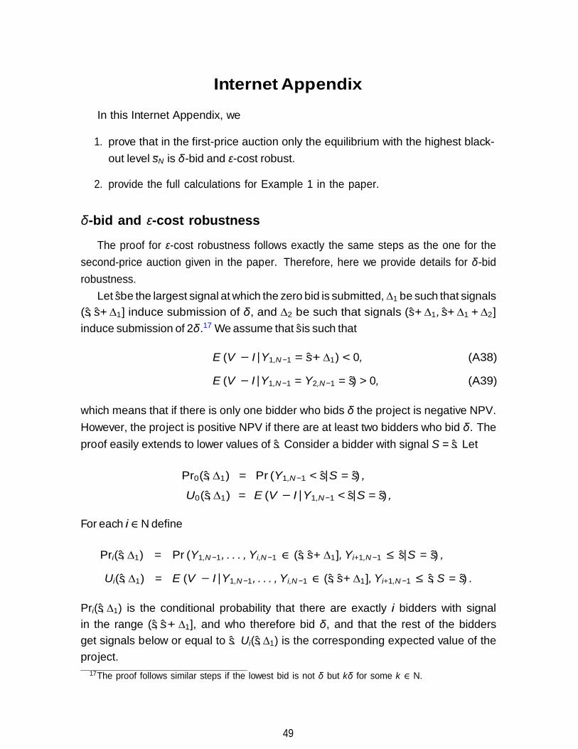
Internet Appendix

In this Internet Appendix, we

1. prove that in the first-price auction only the equilibrium with the highest black- out level sN is δ-bid and ε-cost robust.

2. provide the full calculations for Example 1 in the paper.

δ-bid and ε-cost robustness

The proof for ε-cost robustness follows exactly the same steps as the one for the

second-price auction given in the paper. Therefore, here we provide details for δ-bid robustness.

Let s be the largest signal at which the zero bid is submitted, ∆1 be such that signals (s, s + ∆1] induce submission of δ, and ∆2 be such that signals (s + ∆1, s + ∆1 + ∆2] induce submission of 2δ.17 We assume that s is such that

E (V − I|Y1,N −1 = s + ∆1) < 0, (A38)

E (V − I|Y1,N −1 = Y2,N −1 = s) > 0, (A39) which means that if there is only one bidder who bids δ the project is negative NPV. However, the project is positive NPV if there are at least two bidders who bid δ. The proof easily extends to lower values of s. Consider a bidder with signal S = s. Let

Pr0(s, ∆1) = Pr (Y1,N −1 < s|S = s) ,

U0(s, ∆1) = E (V − I|Y1,N −1 < s|S = s) ,

For each i ∈ N define

Pri(s, ∆1) = Pr (Y1,N −1, . . . , Yi,N −1 ∈ (s, s + ∆1], Yi+1,N −1 ≤ s|S = s) ,

Ui(s, ∆1) = E (V − I|Y1,N −1, . . . , Yi,N −1 ∈ (s, s + ∆1], Yi+1,N −1 ≤ s, S = s) . Pri(s, ∆1) is the conditional probability that there are exactly i bidders with signal in the range (s, s + ∆1], and who therefore bid δ, and that the rest of the bidders get signals below or equal to s. Ui(s, ∆1) is the corresponding expected value of the project.

17The proof follows similar steps if the lowest bid is not δ but kδ for some k ∈ N.

49

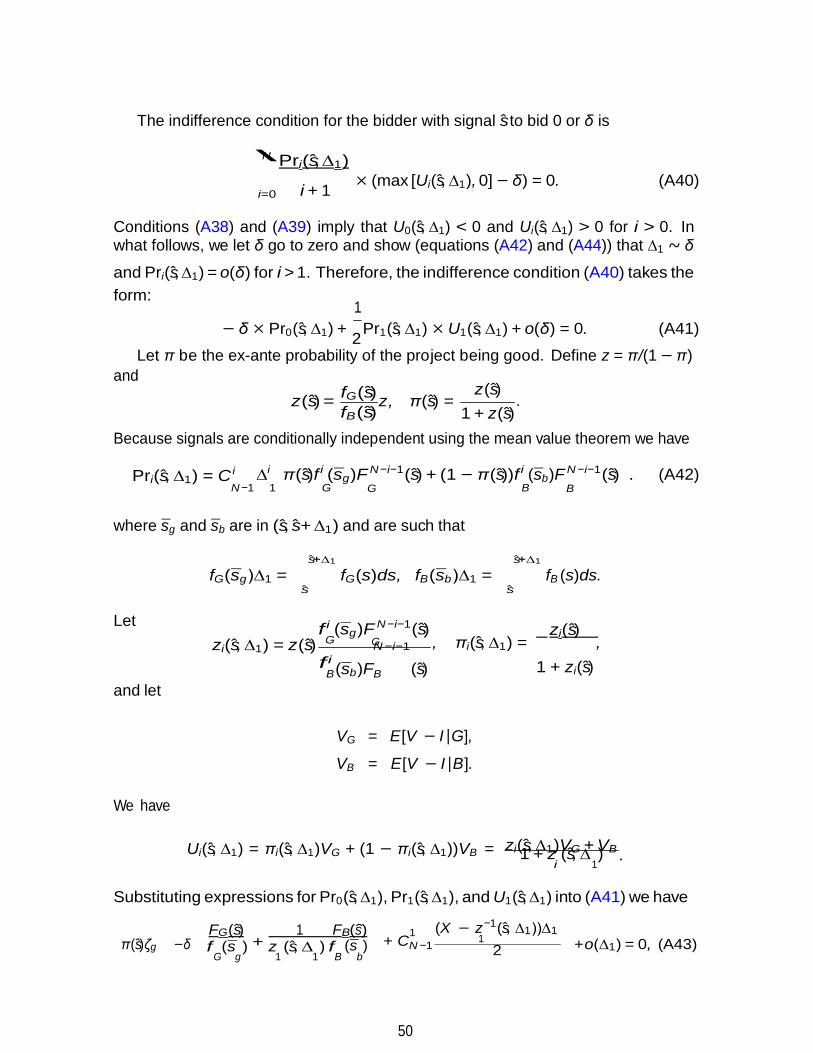
N

1

The indifference condition for the bidder with signal s to bid 0 or δ is

\ Pri(s, ∆1)

i + 1 × (max [Ui(s, ∆1), 0] − δ) = 0. (A40) i=0

Conditions (A38) and (A39) imply that U0(s, ∆1) < 0 and Ui(s, ∆1) > 0 for i > 0. In what follows, we let δ go to zero and show (equations (A42) and (A44)) that ∆1 ∼ δ

and Pri(s, ∆1) = o(δ) for i > 1. Therefore, the indifference condition (A40) takes the form:

1 − δ × Pr0(s, ∆1) + 2 Pr1(s, ∆1) × U1(s, ∆1) + o(δ) = 0. (A41)

Let π be the ex-ante probability of the project being good. Define z = π/(1 − π) and

z(s) = fG(s) fB (s)

z, π(s) = z(s)

. 1 + z(s)

Because signals are conditionally independent using the mean value theorem we have

Pri(s, ∆1) = Ci ∆i π(s)f i (sg )F N −i−1(s) + (1 − π(s))f i (sb)F N −i−1(s) . (A42) N −1 1 G G B B

where sg and sb are in (s, s + ∆1) and are such that

fG(sg )∆1 = s+∆1

s

fG(s)ds, fB (sb)∆1 =

s+∆1

s

fB (s)ds.

Let f i (sg )F N −i−1(s)

zi(s)

zi(s, ∆1) = z(s) G f i

G N −i−1 , πi(s, ∆1) = ,

and let B (sb)FB (s) 1 + zi(s)

VG = E[V − I|G],

VB = E[V − I|B]. We have

Ui(s, ∆1) = πi(s, ∆1)VG + (1 − πi(s, ∆1))VB =

zi(s, ∆1)VG + VB . 1 + z (s, ∆ ) i 1

Substituting expressions for Pr0(s, ∆1), Pr1(s, ∆1), and U1(s, ∆1) into (A41) we have

FG(s) 1 FB (s)

1 (X − z−1(s, ∆1))∆1

π(s)ζg −δ + f (s ) z (s, ∆ ) f (s ) + CN −1 2 +o(∆1) = 0, (A43)

G g 1 1 B b

50

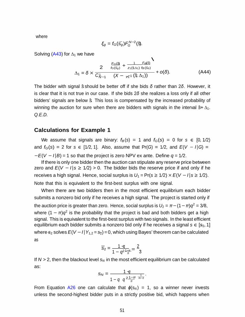
G

C z−1

π

1 − q q

.

where Solving (A43) for ∆1 we have

ξg = fG(sg )F N −2(s).

FG(s) 1 FB (s) \

2 fG(sg ) + z1(s,∆1) fB (sb)

∆1 = δ × 1 N −1 (X −

1 (s, ∆1)) + o(δ). (A44)

The bidder with signal s should be better off if she bids δ rather than 2δ. However, it is clear that it is not true in our case. If she bids 2δ she realizes a loss only if all other bidders’ signals are below s. This loss is compensated by the increased probability of winning the auction for sure when there are bidders with signals in the interval s+ ∆1. Q.E.D.

Calculations for Example 1

We assume that signals are binary: fB (s) = 1 and fG(s) = 0 for s ∈ [0, 1/2) and fG(s) = 2 for s ∈ [1/2, 1]. Also, assume that Pr(G) = 1/2, and E(V − I|G) =

−E(V − I|B) = 1 so that the project is zero NPV ex ante. Define q = 1/2. If there is only one bidder then the auction can stipulate any reserve price between

zero and E(V − I|s ≥ 1/2) > 0. The bidder bids the reserve price if and only if he receives a high signal. Hence, social surplus is U1 = Pr(s ≥ 1/2) × E(V − I|s ≥ 1/2).

Note that this is equivalent to the first-best surplus with one signal. When there are two bidders then in the most efficient equilibrium each bidder

submits a nonzero bid only if he receives a high signal. The project is started only if

the auction price is greater than zero. Hence, social surplus is U2 = π − (1−π)q2 = 3/8, where (1 − π)q2 is the probability that the project is bad and both bidders get a high signal. This is equivalent to the first-best surplus with two signals. In the least efficient equilibrium each bidder submits a nonzero bid only if he receives a signal s ∈ [s2, 1] where s2 solves E(V − I|Y1,2 = s2) = 0, which using Bayes’ theorem can be calculated as

s2 = 1 − q = 2 . 1 − q2 1−π 3

If N > 2, then the blackout level sN in the most efficient equilibrium can be calculated as:

sN = 1 − q 1

2 1−π N −2 π

From Equation A26 one can calculate that ϕ(sN ) = 1, so a winner never invests unless the second-highest bidder puts in a strictly positive bid, which happens when

51

1 − q q

.

Y2,N > sN . We can then calculate the surplus as:

UN (sN ) = π Pr (Y2,N > sN |G) − (1 − π) Pr (Y2,N > sN |B) . Similarly, if N > 2, the blackout level sN in the least efficient equilibrium can be calculated from (4) as:

Therefore,

sN = 1 − q 1

1−π N −1 π

UN (sN ) = π Pr ({Y1,N > sN }|G) − (1 − π) Pr ({Y1,N > sN }|B) .

52

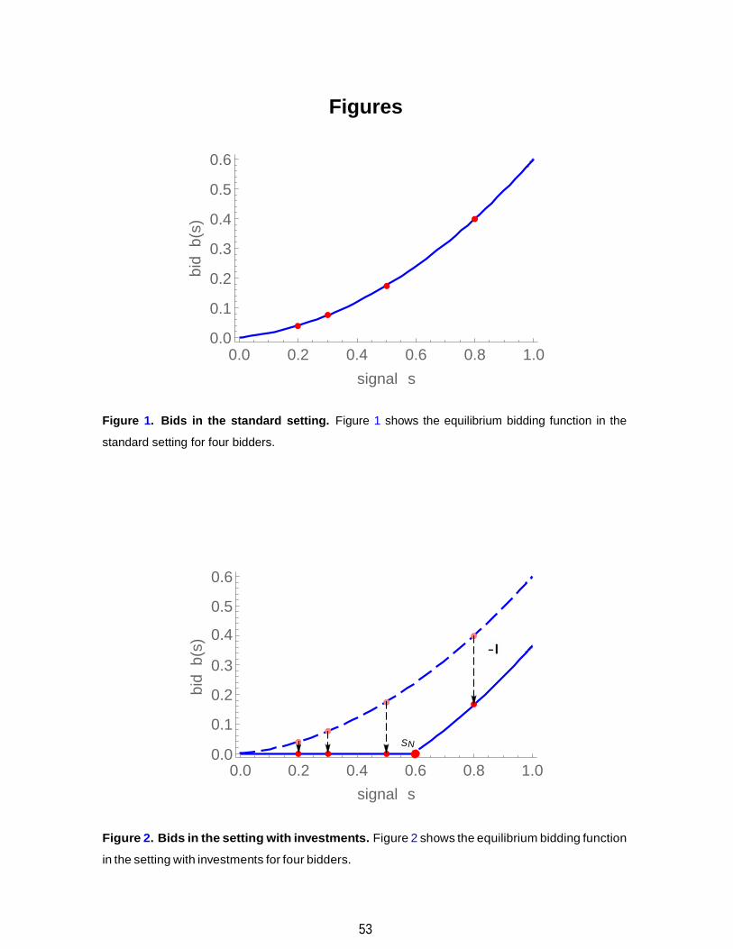
bid

b(s

) bi

d b

(s)

Figures

0.6

0.5

0.4

0.3

0.2

0.1

0.0 0.0 0.2 0.4 0.6 0.8 1.0

signal s Figure 1. Bids in the standard setting. Figure 1 shows the equilibrium bidding function in the

standard setting for four bidders.

0.6

0.5

0.4 -I

0.3

0.2

0.1 SN

0.0 0.0 0.2 0.4 0.6 0.8 1.0

signal s Figure 2. Bids in the setting with investments. Figure 2 shows the equilibrium bidding function

in the setting with investments for four bidders.

53

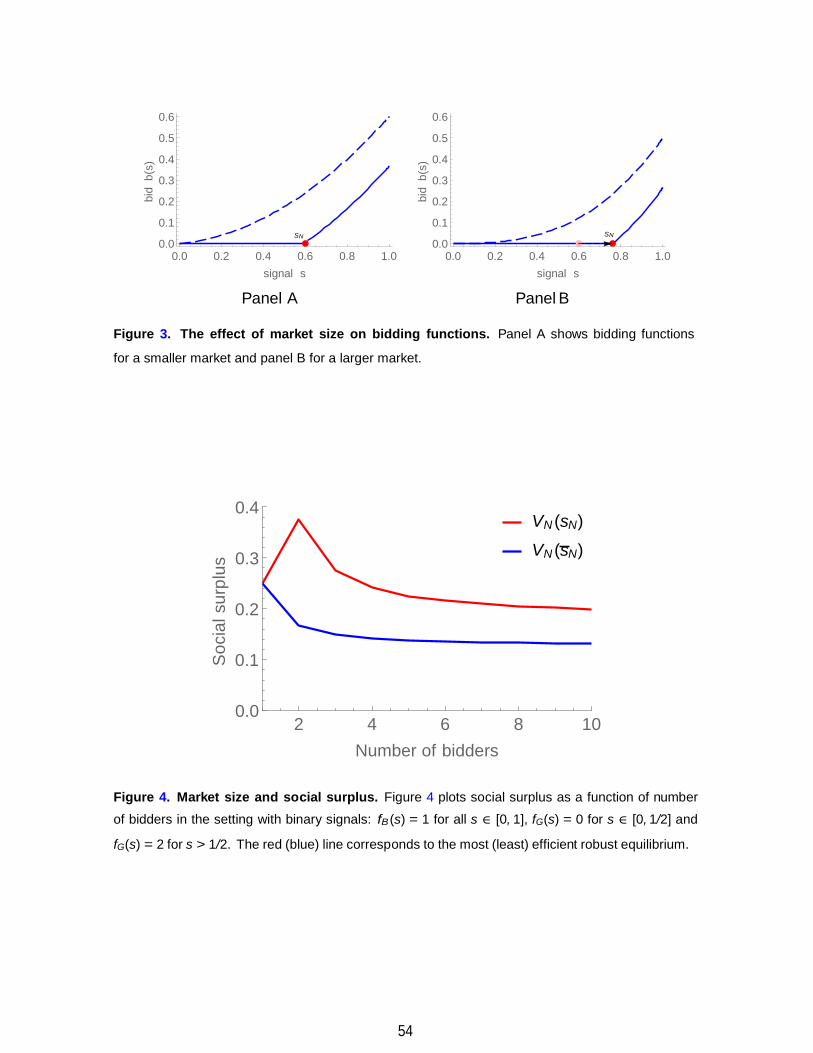
bid

b(s

)

Soc

ial s

urpl

us

bid

b(s

)

0.6 0.6 0.5 0.5 0.4 0.4 0.3 0.3 0.2 0.2 0.1 0.1

0.0 SN

0.0 SN 0.0 0.2 0.4 0.6 0.8 1.0 0.0 0.2 0.4 0.6 0.8 1.0

signal s signal s

Panel A Panel B Figure 3. The effect of market size on bidding functions. Panel A shows bidding functions

for a smaller market and panel B for a larger market.

0.4

0.3

VN (sN)

VN (sN)

0.2

0.1

0.0 2 4 6 8 10

Number of bidders Figure 4. Market size and social surplus. Figure 4 plots social surplus as a function of number

of bidders in the setting with binary signals: fB (s) = 1 for all s ∈ [0, 1], fG(s) = 0 for s ∈ [0, 1/2] and

fG(s) = 2 for s > 1/2. The red (blue) line corresponds to the most (least) efficient robust equilibrium.

54

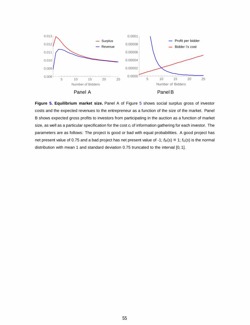
5 10 15 20 25 5 10 15 20 25

Number of Bidders Number of Bidders

0.013

0.012

0.011

Surplus

Revenue

0.0001

0.00008

0.00006

Profit per bidder

Bidder i's cost

0.010 0.00004

0.009 0.00002

0.008

0.0000

Panel A Panel B

Figure 5. Equilibrium market size. Panel A of Figure 5 shows social surplus gross of investor

costs and the expected revenues to the entrepreneur as a function of the size of the market. Panel

B shows expected gross profits to investors from participating in the auction as a function of market

size, as well as a particular specification for the cost ci of information gathering for each investor. The

parameters are as follows: The project is good or bad with equal probabilities. A good project has

net present value of 0.75 and a bad project has net present value of -1; fB (s) ≡ 1; fG(s) is the normal

distribution with mean 1 and standard deviation 0.75 truncated to the interval [0, 1].

55