econstorMake Your Publications Visible.

A Service of

zbwLeibniz-InformationszentrumWirtschaftLeibniz Information Centrefor Economics

Mueller, Andreas I.

Working Paper

Separations, sorting and cyclical unemployment

IZA Discussion Papers, No. 6849

Provided in Cooperation with:IZA – Institute of Labor Economics

Suggested Citation: Mueller, Andreas I. (2012) : Separations, sorting and cyclicalunemployment, IZA Discussion Papers, No. 6849, Institute for the Study of Labor (IZA), Bonn

This Version is available at:http://hdl.handle.net/10419/67208

Standard-Nutzungsbedingungen:

Die Dokumente auf EconStor dürfen zu eigenen wissenschaftlichenZwecken und zum Privatgebrauch gespeichert und kopiert werden.

Sie dürfen die Dokumente nicht für öffentliche oder kommerzielleZwecke vervielfältigen, öffentlich ausstellen, öffentlich zugänglichmachen, vertreiben oder anderweitig nutzen.

Sofern die Verfasser die Dokumente unter Open-Content-Lizenzen(insbesondere CC-Lizenzen) zur Verfügung gestellt haben sollten,gelten abweichend von diesen Nutzungsbedingungen die in der dortgenannten Lizenz gewährten Nutzungsrechte.

Terms of use:

Documents in EconStor may be saved and copied for yourpersonal and scholarly purposes.

You are not to copy documents for public or commercialpurposes, to exhibit the documents publicly, to make thempublicly available on the internet, or to distribute or otherwiseuse the documents in public.

If the documents have been made available under an OpenContent Licence (especially Creative Commons Licences), youmay exercise further usage rights as specified in the indicatedlicence.

www.econstor.eu

DI

SC

US

SI

ON

P

AP

ER

S

ER

IE

S

Forschungsinstitut zur Zukunft der ArbeitInstitute for the Study of Labor

Separations, Sorting and Cyclical Unemployment

IZA DP No. 6849

September 2012

Andreas I. Mueller

Separations, Sorting and Cyclical Unemployment

Andreas I. Mueller Columbia University

and IZA

Discussion Paper No. 6849 September 2012

IZA

P.O. Box 7240 53072 Bonn

Germany

Phone: +49-228-3894-0 Fax: +49-228-3894-180

E-mail: iza@iza.org

Any opinions expressed here are those of the author(s) and not those of IZA. Research published in this series may include views on policy, but the institute itself takes no institutional policy positions. The Institute for the Study of Labor (IZA) in Bonn is a local and virtual international research center and a place of communication between science, politics and business. IZA is an independent nonprofit organization supported by Deutsche Post Foundation. The center is associated with the University of Bonn and offers a stimulating research environment through its international network, workshops and conferences, data service, project support, research visits and doctoral program. IZA engages in (i) original and internationally competitive research in all fields of labor economics, (ii) development of policy concepts, and (iii) dissemination of research results and concepts to the interested public. IZA Discussion Papers often represent preliminary work and are circulated to encourage discussion. Citation of such a paper should account for its provisional character. A revised version may be available directly from the author.

IZA Discussion Paper No. 6849 September 2012

ABSTRACT

Separations, Sorting and Cyclical Unemployment* This paper establishes a new fact about the compositional changes in the pool of unemployed over the U.S. business cycle and evaluates a number of theories that can potentially explain it. Using micro-data from the Current Population Survey for the years 1962-2011, it documents that in recessions the pool of unemployed shifts towards workers with high wages in their previous job. Moreover, it shows that these changes in the composition of the unemployed are mainly due to the higher cyclicality of separations for high-wage workers, and not driven by differences in the cyclicality of job-finding rates. A search-matching model with endogenous separations and worker heterogeneity in terms of ability has difficulty in explaining these patterns, but an extension of the model with credit-constraint shocks does much better in accounting for the new facts. JEL Classification: E24, E32, J63 Keywords: sorting, unemployment, business cycles, search-matching, vacancies Corresponding author: Andreas I. Mueller Columbia Business School Columbia University Uris Hall 3022 Broadway New York, NY 10027 USA E-mail: amueller@columbia.edu

* I am grateful to Per Krusell, John Hassler, Torsten Persson, Alan B. Krueger, Mark Aguiar, Dale Mortensen, Jonathan Parker, Mark Bils, Yongsung Chang, Erik Hurst, Thijs van Rens, Fabrizio Zilibotti, Pascal Michaillat, Aysegul Sahin, Mike Elsby, Almut Balleer, Phillippe Aghion, Valerie A. Ramey, Toshihiko Mukoyama, Gueorgui Kambourov, Guillermo Ordonez, Steinar Holden, Tobias Broer, Ethan Kaplan, Mirko Abbritti, Shon Ferguson, David von Below, Erik Meyersson, Daniel Spiro, Ronny Freier and participants at seminars at Columbia GSB, Northwestern University, the University of Edinburgh, the Federal Reserve Bank of Richmond, the Federal Reserve Bank of New York, the University of Western Ontario, Toulouse School of Economics, Aarhus University, the University of Essex, the University of Southampton, the University of Lausanne, McGill University, University of Montreal, the Bank of England, the NordMac symposium 2010 and the Econometric Society European Winter Meeting for very helpful comments and ideas, and to Handelsbanken’s Research Foundations and the Mannerfelt Foundation for financial support.

1 Introduction

This paper establishes a new fact about the compositional changes in the pool of unemployed

over the U.S. business cycle and evaluates a number of theories that can potentially explain

it. Using micro data from the Current Population Survey (CPS) for the years 1962-2011, I

document that in recessions the pool of unemployed shifts towards workers with high wages in

their previous job. This cyclical pattern is robust to many different empirical specifications.

Controlling for observable characteristics such as education, experience, occupation etc. in

the wage, I show that the share of unemployed with high residual wages still increases in

recessions, although the magnitude of the increase is smaller than for the raw wage measure.

This finding suggests that both observed and unobserved factors explain the shift towards

high-wage workers in recessions. I also investigate whether the compositional shift is due to

differences in the cyclicality of separation or job-finding rates across wage groups, and find

that the compositional shift is almost entirely driven by separations.

These empirical patterns may appear to contradict findings from a related literature on

the cyclicality of real wages. Specifically, Solon, Barsky and Parker (1994) documented that

the measured cyclicality of aggregate real wages is downward biased, because the typical

employed person is of higher ability in recessions. Hines, Hoynes and Krueger (2001), how-

ever, showed that Solon, Barsky and Parker’s result relies on the weighting of aggregate real

wages by hours worked. With unweighted wage data, composition bias has almost no effect

on the cyclicality of real wages, suggesting that is not the composition of the employed that

changes over the business cycles but rather the hours worked by different skill groups. More-

over, changes in the composition of the employed do not necessarily translate into changes

in the pool of unemployed in the opposite direction if the average quality between the pools

differs. In fact, I show that large shifts towards high-wage workers in the pool of unemployed

are consistent with small shifts towards high-wage workers in the pool of employed.

My empirical findings have potentially important implications for models of aggregate

fluctuations in the labor market, as changes in the pool of unemployed feed back into firms’

incentives for hiring. Contrary to Pries (2008), who assumes that the pool of unemployed

shifts towards low-ability workers, shifts towards high-ability workers in recessions lead to a

dampening of productivity shocks. The reason is that when unemployment shifts towards

the more able, the probability that a firm finds a worker of high ability goes up, which raises

the returns to posting vacancies. This poses an additional challenge to the recent literature

on the "unemployment volatility puzzle" (see Shimer, 2005), as shifts towards high-ability

workers in recessions may dampen the response of hiring and unemployment to aggregate

productivity shocks.

Given the importance of the new fact I document in the first part of the paper, the second

2

part of the paper tries to explain it. For this purpose, I first set up a search-matching model

with match-specific productivity shocks, endogenous separations and worker heterogeneity

in terms of ability.1 The baseline model, however, implies shifts in the pool of unemployed

towards low-ability workers in recessions, which is inconsistent with the new facts. I also

explore other calibrations of the model, as well as models with different types of worker

heterogeneities such as differences in bargaining power or home production. All these models,

however, have diffi culties in replicating the key facts summarized above. Therefore, I offer two

extensions of the model that can potentially explain the more cyclical nature of separations

for high-ability workers.

One explanation is that many layoffs in downturns occur due to firm and plant death.

These shocks affect workers indiscriminately of type and thus lead to larger increases in sep-

arations in percentage terms for those with lower average separation rates (i.e., high-ability

workers). The model, however, cannot fully explain the higher cyclicality of separations for

high-ability workers because these firm death shocks are not cyclical enough.

Thus, I propose another extension of the model with credit shocks, where firms are

constrained to produce positive cash flows in recessions. This also produces more cyclical

separations for high-ability workers. The idea is that it is more diffi cult to obtain outside

financing in recessions as liquidity dries up in financial markets. In the baseline model with

effi cient separations, worker-firm matches produce negative cash flows at the productivity

threshold where separations occur. The firm is willing to pay the worker above current

match productivity, because it is compensated by expected positive future cash flows. Thus,

if firms face constraints on their cash flows in recessions, workers and firms may separate

even though it would be in the interest of both parties to continue the relationship. This

mechanism is stronger for high-ability workers, because they produce larger negative cash

flows at the effi cient (unconstrained) separation threshold. Therefore, separations of these

workers are more sensitive to a tightening of credit. As a result, the model produces more

cyclical separations for high-ability workers, consistent with the empirical patterns in the

U.S. data.

The remainder of the paper is organized as follows. Section 2 describes the CPS data and

carries out the empirical analysis. Section 3 sets up the search-matching model, discusses

alternative calibration strategies, and studies the model with firm and plant death. Section

4 extends the model with credit-constraint shocks and Section 5 concludes the paper.

1Bils, Chang and Kim (2012) also study the cyclicality of separations for different wage and hours groups.However, they pay little attention to compositional changes in the pool of unemployed. See also Section2 below for a discussion of their empirical results from the Survey of Income and Program Participation(SIPP).

3

2 Data

The empirical analysis in this paper is based on U.S. micro data from the Current Population

Survey (CPS) for the period 1962-2011. The CPS is the main labor force survey for the

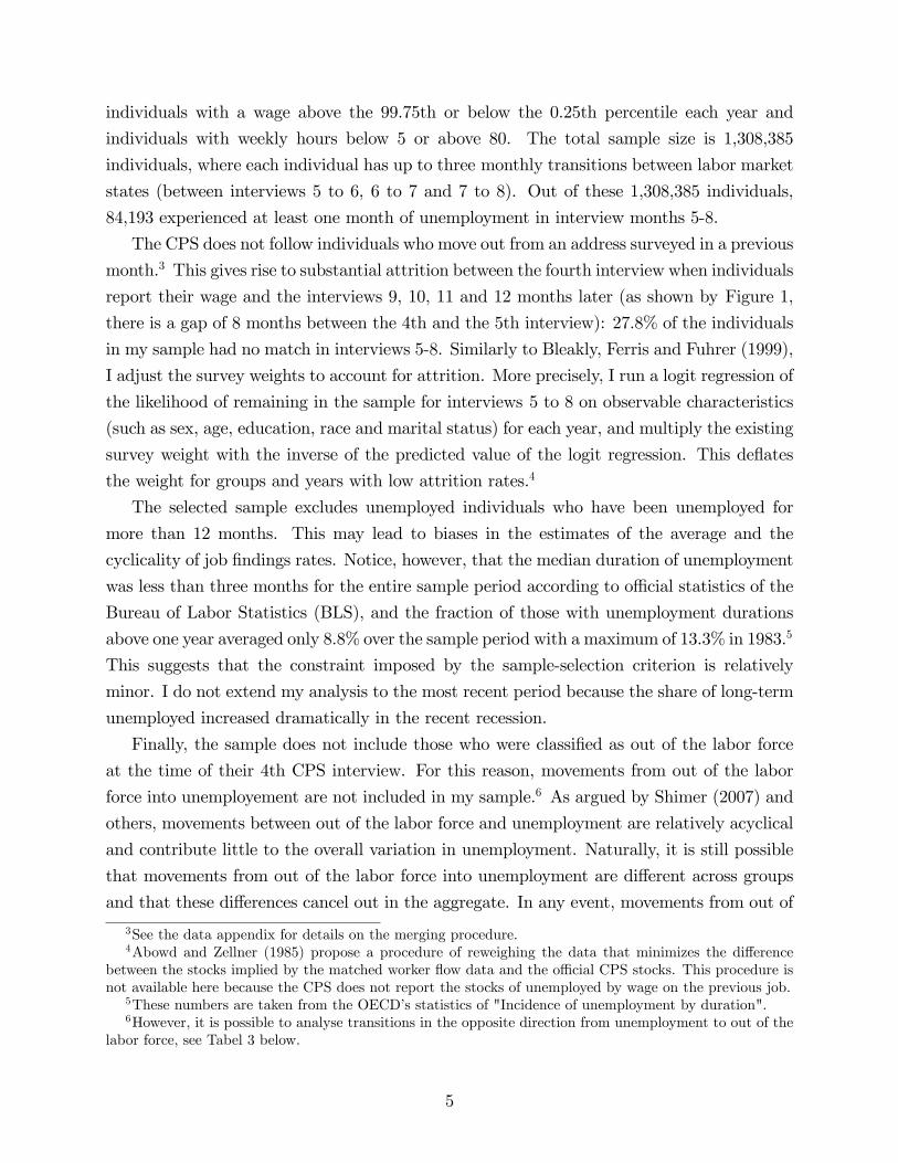
U.S., representative of the population aged 15 and older. It has a rotating panel structure,

where households are surveyed in four consecutive months, rotated out of the panel for

eight months, and then surveyed again for another four consecutive months, as illustrated

in Figure 1. Note that the CPS records the labor-force status for each person in the sample

each month. Weekly hours and earnings, however, are collected only in the fourth and eighth

interview of the survey, referred to as the Outgoing Rotation Groups (ORG).

Figure 1: CPS panel structure by month and interview numberMonth

InterviewWage Wage

1 2 3 4 5 6 7 814 15 169 10 12 13115 6 7 81 2 3 4

The empirical analysis proceeds with two different data sources: First, I use data from the

CPS ORG and monthly files to estimate monthly transition probabilities from employment

to unemployment and vice versa for the period 1979-2008. Second, to extend the analysis

to the period before 1979, I use data from the CPS March supplement for the period 1962-

2011. The march supplement collects data on wage income from the last year for those

currently unemployed, and can be used to replicate the main statistic of the compositional

changes in the pool of unemployed, but it does not allow for an analysis of monthly transition

probabilities as it is collected only once per year.

2.1 Sample Criteria and Measurement

CPS Outgoing Rotation Group (ORG) and monthly data (1979-2008) The main

focus of the empirical analysis is on the wage of those who lose their job and become unem-

ployed. Wage data is available only for the fourth and the eighth interview of each household.

I restrict my sample to all individuals with available wage data from the fourth interview and

analyze the employment outcomes in subsequent months. I do not use wage data from the

eighth interview as this is the final interview in the CPS panel and I want to avoid possible

selection effects associated with including wages after job loss.2

I restrict my sample to individuals aged 19 to 64 who worked in the private sector, are

not self-employed and not self-incorporated. I also trim the sample for outliers excluding

2The main concern is that individuals who separate in recessions tend to have lower wages on their newjob, because it has been documented that wages for new hires are more responsive to the business cycle.See, e.g., Bils (1985) or, more recently, Haefke, Sonntag and van Rens (2012).

4

individuals with a wage above the 99.75th or below the 0.25th percentile each year and

individuals with weekly hours below 5 or above 80. The total sample size is 1,308,385

individuals, where each individual has up to three monthly transitions between labor market

states (between interviews 5 to 6, 6 to 7 and 7 to 8). Out of these 1,308,385 individuals,

84,193 experienced at least one month of unemployment in interview months 5-8.

The CPS does not follow individuals who move out from an address surveyed in a previous

month.3 This gives rise to substantial attrition between the fourth interview when individuals

report their wage and the interviews 9, 10, 11 and 12 months later (as shown by Figure 1,

there is a gap of 8 months between the 4th and the 5th interview): 27.8% of the individuals

in my sample had no match in interviews 5-8. Similarly to Bleakly, Ferris and Fuhrer (1999),

I adjust the survey weights to account for attrition. More precisely, I run a logit regression of

the likelihood of remaining in the sample for interviews 5 to 8 on observable characteristics

(such as sex, age, education, race and marital status) for each year, and multiply the existing

survey weight with the inverse of the predicted value of the logit regression. This deflates

the weight for groups and years with low attrition rates.4

The selected sample excludes unemployed individuals who have been unemployed for

more than 12 months. This may lead to biases in the estimates of the average and the

cyclicality of job findings rates. Notice, however, that the median duration of unemployment

was less than three months for the entire sample period according to offi cial statistics of the

Bureau of Labor Statistics (BLS), and the fraction of those with unemployment durations

above one year averaged only 8.8% over the sample period with a maximum of 13.3% in 1983.5

This suggests that the constraint imposed by the sample-selection criterion is relatively

minor. I do not extend my analysis to the most recent period because the share of long-term

unemployed increased dramatically in the recent recession.

Finally, the sample does not include those who were classified as out of the labor force

at the time of their 4th CPS interview. For this reason, movements from out of the labor

force into unemployement are not included in my sample.6 As argued by Shimer (2007) and

others, movements between out of the labor force and unemployment are relatively acyclical

and contribute little to the overall variation in unemployment. Naturally, it is still possible

that movements from out of the labor force into unemployment are different across groups

and that these differences cancel out in the aggregate. In any event, movements from out of

3See the data appendix for details on the merging procedure.4Abowd and Zellner (1985) propose a procedure of reweighing the data that minimizes the difference

between the stocks implied by the matched worker flow data and the offi cial CPS stocks. This procedure isnot available here because the CPS does not report the stocks of unemployed by wage on the previous job.

5These numbers are taken from the OECD’s statistics of "Incidence of unemployment by duration".6However, it is possible to analyse transitions in the opposite direction from unemployment to out of the

labor force, see Tabel 3 below.

5

the labor force into unemployment are another potential margin of cyclical changes in the

composition of the pool of unemployed, which is omitted from my analysis.

CPS March supplement (1962-2011) As mentioned above, I extend the analysis from

the CPS ORG and monthly data with data from the CPS March supplement, which is

available since 1962. Besides the extended sample period, an additional advantage of the

March supplement is that it does not rely on matching individuals across different interviews,

since data on wages on the previous job are available from the same interview. Thus, it

provides a direct test of whether differential attrition by wage group is biasing my results in

the analysis with the CPS monthly interview data. A further advantage of the analysis with

the CPS March supplement is that it includes any person that had positive earnings during

the last calendar year and, thus, includes individuals who have been unemployed for up to

14.5 months compared to 12 months for the monthly data (the interview date is in the middle

of the month of March). A weakness, however, of the CPS March supplement is that it is only

available once per year and thus does not allow the analysis of monthly transitions between

employment and unemployment and vice versa. Moreover, it is not possible to compute an

hourly wage over the entire period as for the period before 1976 there is no information on

hours worked and thus I use the weekly wage, defined as the total income from wages and

salary divided by the number of weeks worked during the previous calendar year. Despite

these shortcomings, the CPS March sample allows me to extend the analysis back to 1962

and is a useful robustness check on the analysis with the CPS ORG and monthly data. I

use the same sample restrictions and thresholds for trimming in the CPS March supplement,

and the sample size is 2,237,705 out of which 135,708 were unemployed at the time of the

March interview.

2.2 The Cyclicality of the Wage of Job Losers

Does the composition of the unemployed change over the business cycle? Are there changes

in the pool of unemployed by ability? To answer these questions, I use the wage on the

previous job as a summary indicator of compositional changes in the pool of unemployed.

Panel (a) in Figure 2 plots the average wage of those who lost their job in the previous year,

as well as the average wage of those who remained employed. More precisely, it shows the

average wage for those who were employed in interview 4 but unempoyed in interview 8 of

the CPS, as well as the average wage of those who remained employed. As is apparent from

the plot, the average wage of the unemployed is strongly and positively correlated with the

6

aggregate unemployment rate (the correlation coeffi cient is 0.55).7 ,8 Panel (a) in Figure 3

shows very similar patterns for the cyclicality of the average wage on previous job, using the

CPS March sample over the period 1962-2011. The table further shows that the patterns

appear in every single recession since 1962, and the magnitude of the changes is very similar

across the two data sources.9

One might be concerned about wage compression and argue that the wage differential

between those who lose their job and those who remain employed narrows in a recession,

simply because overall wage dispersion becomes smaller at the same time. To evaluate this

possibility, I attribute an ordinal wage rank to each individual in my data set (the rank in

the wage distribution in a given year is defined by lining up all individuals according to their

current wage from the lowest to the highest on the unit interval). If wage compression drives

the patterns in Panel (a) of Figures 2 and 3, then the average wage rank should show no

correlation with the aggregate unemployment rate. However, Panel (b) in the same figures

show a very strong correlation of the average wage rank of the unemployed with the aggregate

unemployment rate. The correlation coeffi cient is 0.72 (CPS March data: 0.74), suggesting

that wage compression plays no role. In terms of the magnitude, a percentage-point increase

in the unemployment rate is, on average, associated with a 1.5 percentage-point increase

(CPS March data: 1.2 percentage-point increase) in the average wage rank of the job losers,

which represents a substantial shift in the composition of the pool of unemployed.

Panel (c) in Figures 2 and 3 shows the same plot but for the residual of a Mincer-

style regression of the log wage on observable characteristics such as potential experience,

educational attainment, gender, marital status, and race, and dummies for state, industry,

occupation and year.10 The average wage residual is still strongly counter-cyclical for those

who lost their job in the previous year, with a correlation with the unemployment rate of

0.58. The magnitude is smaller as a percentage-point increase in the unemployment rate

leads to a 0.90% increase (CPS March data: 0.84%) in the average residual wage of the

unemployed, as compared to a 2.76% increase (CPS March data: 2.88%) in the average raw

wage in Panel (a). This suggests that both observed and unobserved factors contribute to

the compositional changes in the unemployment pool over the business cycle.

To get a better sense of what observable factors drive the compositional changes in the

unemployment pool, I regress the detrended series of each component of the predicted wage

7The unemployment rate is taken from the offi cial tables of the Bureau of Labor Statistics.8One might also note that the compositional changes seem to be slightly leading the unemployment rate.

The reason is that - as documented further below - the changes in the pool are driven by the differentialcyclicality in job separations, which tend to lead the unemployment rate.

9The correlation coeffi cient of the two series over the period 1980-2008 is 0.84.10By definition, the average wage residual is zero for each year for the full sample and close to zero for the

employed as they represent over 90 % of the full sample.

7

Figure 2: The average wage from previous year by employment status in CPS ORG files1980-2008.

­.01

0.0

1.0

2U

nem

ploy

men

t rat

e

­.05

0.0

5.1

log(

prev

ious

 wag

e)

1980 1985 1990 1995 2000 2005

(a) Raw  w age

­.01

0.0

1.0

2U

nem

ploy

men

t rat

e

­.04

­.02

0.0

2.0

4W

age 

rank

1980 1985 1990 1995 2000 2005

(b) Wage rank

­.01

0.0

1.0

2U

nem

ploy

men

t rat

e

­.05

0.0

5.1

log(

prev

ious

 wag

e)

1980 1985 1990 1995 2000 2005

Unemployment ratePrevious w age (Unemployed)Previous w age (Employed)

(c) Mincer­residual

Note: All series are y early  av erages, HP­f iltered with smoothing parameter 100.

8

Figure 3: The average wage from previous year by employment status in CPS March files1962-2011.

­.02

­.01

0.0

1.0

2U

nem

ploy

men

t rat

e

­.08

­.03

.02

.07

.12

log(

prev

ious

 wag

e)

1960 1970 1980 1990 2000 2010

(a) Raw  w age

­.02

­.01

0.0

1.0

2U

nem

ploy

men

t rat

e

­.04

­.02

0.0

2.0

4W

age 

rank

1960 1970 1980 1990 2000 2010

(b) Wage rank

­.02

­.01

0.0

1.0

2U

nem

ploy

men

t rat

e

­.08

­.03

.02

.07

.12

log(

prev

ious

 wag

e)

1960 1970 1980 1990 2000 2010

Unemployment ratePrevious w age (Unemployed)Previous w age (Employed)

(c) Mincer­residual

Note: All series are y early  av erages, HP­f iltered with smoothing parameter 100.

9

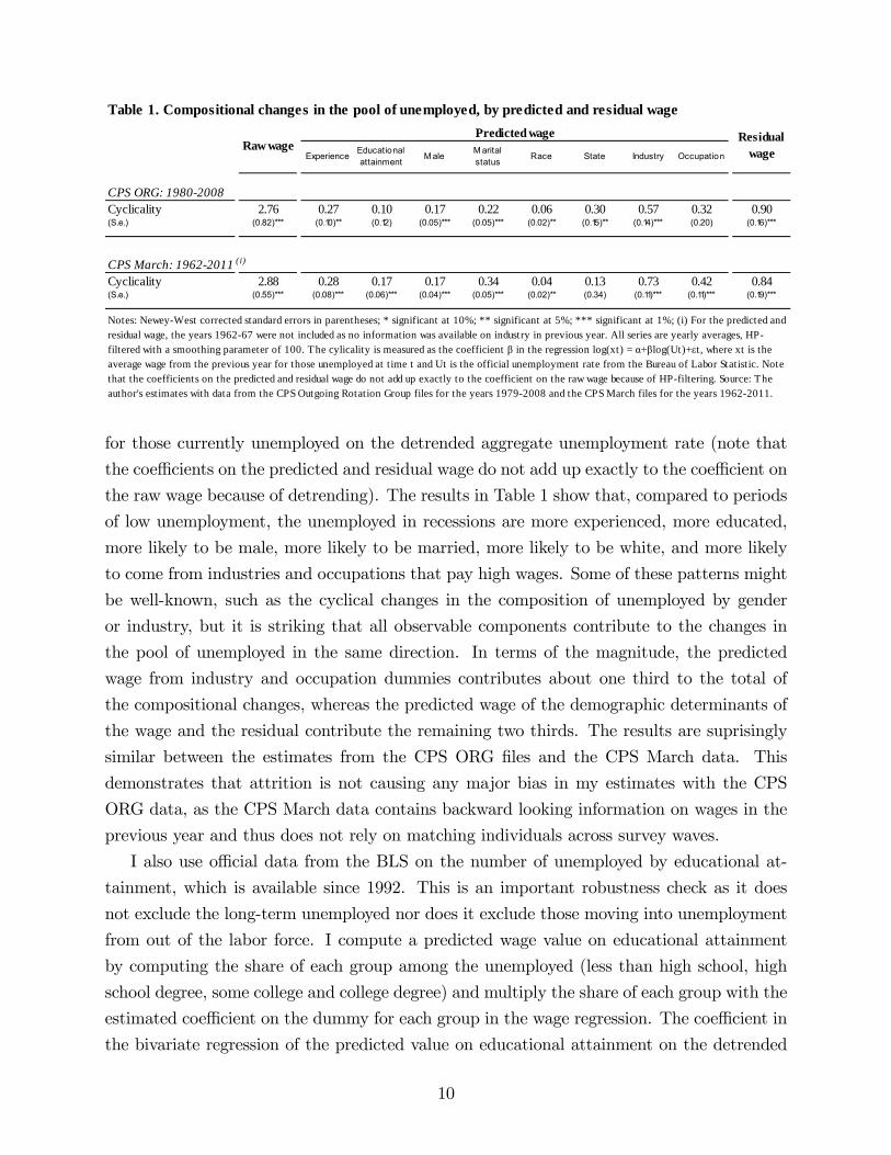
Table 1. Compositional changes in the pool of unemployed, by predicted and residual wage

ExperienceEducationalattainment M ale

M aritalstatus Race State Industry Occupation

CPS ORG: 1980­2008Cyclicality 2.76 0.27 0.10 0.17 0.22 0.06 0.30 0.57 0.32 0.90(S.e.) (0.82)*** (0.10)** (0.12) (0.05)*** (0.05)*** (0.02)** (0.15)** (0.14)*** (0.20) (0.16)***

CPS March: 1962­2011 ( i)

Cyclicality 2.88 0.28 0.17 0.17 0.34 0.04 0.13 0.73 0.42 0.84(S.e.) (0.55)*** (0.08)*** (0.06)*** (0.04)*** (0.05)*** (0.02)** (0.34) (0.11)*** (0.11)*** (0.19)***

Raw wagePredicted wage Residual

wage

Notes: Newey­West corrected standard errors in parentheses; * significant at 10%; ** significant at 5%; *** significant at 1%; (i) For the predicted andresidual wage, the years 1962­67 were not included as no information was available on industry in previous year. All series are yearly averages, HP­filtered with a smoothing parameter of 100. The cylicality is measured as the coefficient β in the regression log(xt) = α+βlog(Ut)+εt , where xt is theaverage wage from the previous year for those unemployed at t ime t and Ut is the official unemployment rate from the Bureau of Labor Statistic. Notethat the coefficients on the predicted and residual wage do not add up exactly to the coefficient  on the raw wage because of HP­filtering. Source: Theauthor's estimates with data from the CPS Outgoing Rotation Group files for the years 1979­2008 and the CPS March files for the years 1962­2011.

for those currently unemployed on the detrended aggregate unemployment rate (note that

the coeffi cients on the predicted and residual wage do not add up exactly to the coeffi cient on

the raw wage because of detrending). The results in Table 1 show that, compared to periods

of low unemployment, the unemployed in recessions are more experienced, more educated,

more likely to be male, more likely to be married, more likely to be white, and more likely

to come from industries and occupations that pay high wages. Some of these patterns might

be well-known, such as the cyclical changes in the composition of unemployed by gender

or industry, but it is striking that all observable components contribute to the changes in

the pool of unemployed in the same direction. In terms of the magnitude, the predicted

wage from industry and occupation dummies contributes about one third to the total of

the compositional changes, whereas the predicted wage of the demographic determinants of

the wage and the residual contribute the remaining two thirds. The results are suprisingly

similar between the estimates from the CPS ORG files and the CPS March data. This

demonstrates that attrition is not causing any major bias in my estimates with the CPS

ORG data, as the CPS March data contains backward looking information on wages in the

previous year and thus does not rely on matching individuals across survey waves.

I also use offi cial data from the BLS on the number of unemployed by educational at-

tainment, which is available since 1992. This is an important robustness check as it does

not exclude the long-term unemployed nor does it exclude those moving into unemployment

from out of the labor force. I compute a predicted wage value on educational attainment

by computing the share of each group among the unemployed (less than high school, high

school degree, some college and college degree) and multiply the share of each group with the

estimated coeffi cient on the dummy for each group in the wage regression. The coeffi cient in

the bivariate regression of the predicted value on educational attainment on the detrended

10

aggregate unemployment rate is 0.24 (with a standard error of 0.09), which is a little bit

higher than the estimates on the predicted value by educational attainment in Table 1, but

within the confidence interval. The compositional changes by educational attainment might

come as a surprise to some, as the unemployment rate tends to be much more volatile for

the low skilled. However, as demonstrated further below, it is the volatility of the log of the

unemployment rate, and not the volatility of the level, that matters for the compositional

changes in the pool of unemployed.

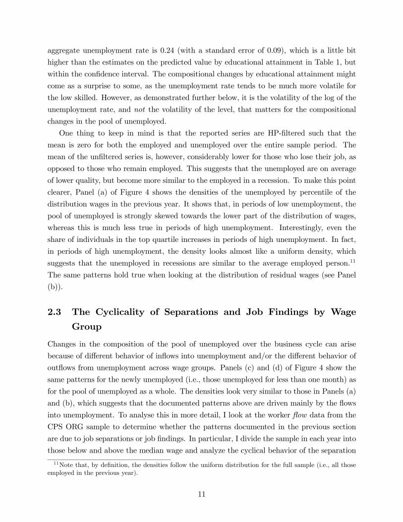
One thing to keep in mind is that the reported series are HP-filtered such that the

mean is zero for both the employed and unemployed over the entire sample period. The

mean of the unfiltered series is, however, considerably lower for those who lose their job, as

opposed to those who remain employed. This suggests that the unemployed are on average

of lower quality, but become more similar to the employed in a recession. To make this point

clearer, Panel (a) of Figure 4 shows the densities of the unemployed by percentile of the

distribution wages in the previous year. It shows that, in periods of low unemployment, the

pool of unemployed is strongly skewed towards the lower part of the distribution of wages,

whereas this is much less true in periods of high unemployment. Interestingly, even the

share of individuals in the top quartile increases in periods of high unemployment. In fact,

in periods of high unemployment, the density looks almost like a uniform density, which

suggests that the unemployed in recessions are similar to the average employed person.11

The same patterns hold true when looking at the distribution of residual wages (see Panel

(b)).

2.3 The Cyclicality of Separations and Job Findings by Wage

Group

Changes in the composition of the pool of unemployed over the business cycle can arise

because of different behavior of inflows into unemployment and/or the different behavior of

outflows from unemployment across wage groups. Panels (c) and (d) of Figure 4 show the

same patterns for the newly unemployed (i.e., those unemployed for less than one month) as

for the pool of unemployed as a whole. The densities look very similar to those in Panels (a)

and (b), which suggests that the documented patterns above are driven mainly by the flows

into unemployment. To analyse this in more detail, I look at the worker flow data from the

CPS ORG sample to determine whether the patterns documented in the previous section

are due to job separations or job findings. In particular, I divide the sample in each year into

those below and above the median wage and analyze the cyclical behavior of the separation

11Note that, by definition, the densities follow the uniform distribution for the full sample (i.e., all thoseemployed in the previous year).

11

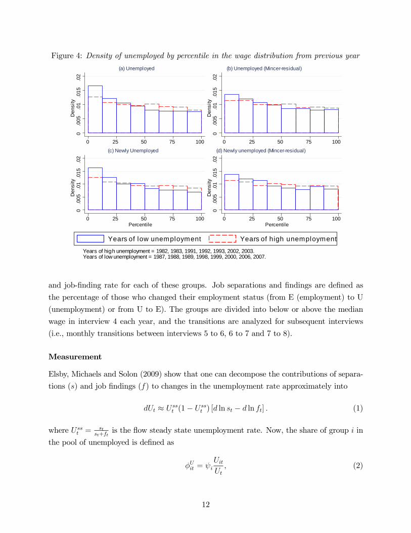
Figure 4: Density of unemployed by percentile in the wage distribution from previous year

0.0

05.0

1.0

15.0

2D

ensi

ty

0 25 50 75 100

(a) Unemployed

0.0

05.0

1.0

15.0

2D

ensi

ty

0 25 50 75 100

(b) Unemployed (Mincer­residual)

0.0

05.0

1.0

15.0

2D

ensi

ty

0 25 50 75 100Percentile

(c) Newly Unemployed

0.0

05.0

1.0

15.0

2D

ensi

ty

0 25 50 75 100Percentile

(d) Newly unemployed (Mincer­residual)

         Years of high unemployment = 1982, 1983, 1991, 1992, 1993, 2002, 2003.         Years of low unemployment = 1987, 1988, 1989, 1998, 1999, 2000, 2006, 2007.

Years of low unemployment Years of high unemployment

and job-finding rate for each of these groups. Job separations and findings are defined as

the percentage of those who changed their employment status (from E (employment) to U

(unemployment) or from U to E). The groups are divided into below or above the median

wage in interview 4 each year, and the transitions are analyzed for subsequent interviews

(i.e., monthly transitions between interviews 5 to 6, 6 to 7 and 7 to 8).

Measurement

Elsby, Michaels and Solon (2009) show that one can decompose the contributions of separa-

tions (s) and job findings (f) to changes in the unemployment rate approximately into

dUt ≈ U sst (1− U ss

t ) [d ln st − d ln ft] . (1)

where U sst = st

st+ftis the flow steady state unemployment rate. Now, the share of group i in

the pool of unemployed is defined as

φUit = ψiUitUt, (2)

12

where Uit is the unemployment rate of group i at time t and ψi is the population share for

group i (assumed to be constant). Given equations (1) and (2), it can be shown that changes

in the share of group i in the pool of unemployed can be decomposed into

dφUit ≈ φUit

((1− U ss

it ) [d ln sit − d ln fit]

−(1− U sst ) [d ln st − d ln ft]

), (3)

which implies that changes in the share of group i are related to changes in the log of the

separation and job-finding rate of group i relative to the average. More importantly, since

(1−U ssit ) is very similar across groups, one can directly conclude from the magnitude of the

changes in the log separation and job-finding rates which margins are more important for

the changes in the composition of the pool. To understand how separations and job findings

relate to cyclical changes in the unemployment rate, one thus has to relate the changes in

the log of the separation and job-finding rate to the aggregate unemployment rate (or other

cyclical indicators). For this reason, I run the following regressions:

lnxit = αxi + βxi lnUt + εxit, (4)

where xit stands for sit (separation rate), fit (job-finding rate) or Uit (unemployment rate)

for group i at time t and the measure of cyclicality is the percent increase in xit in response

to a 1% increase in the aggregate unemployment rate (the coeffi cient βxi ). All series are

monthly, seasonally adjusted, and detrended with an HP-filter with smoothing parameter

900,000.12

Results

Table 2 summarizes the main results for different groups in terms of the average as well as

the cyclicality of separation and job-finding rates. The first two columns split the sample

into those below and above the median wage. Columns 3 and 4 report the results for those

below and above the median residual wage.

Not surprisingly, separations are on average lower for high-wage workers than for low-

wage workers. The main new result, however, is that the cyclicality of separations is almost

twice as large for individuals with high wages compared to those below the median.13 The

12I follow Bils, Chang and Kim (2009) who detrend the monthly time series with an HP-filter with smooth-ing parameter 900,000. This is the equivalent of Shimer’s (2005) detrending choice of a smoothing parameterof 100,000 for a quarterly time series. The published version of Bils, Chang and Kim (2012) does no longerfollow this detrending choice. Appendix Tables A.1-A.3 show that my results are robust to other detrendingmethods, and in particular to HP-filtering with a smoothing parameter of 14,400.13My results are also consistent with Fujita and Ramey’s (2009) analysis who show that - using CPS

worker flow data from 1976 to 2005 - that separations account for approximately 50% of the overall volatility

13

low high low highSeparations Average 0.012 0.007 0.010 0.008

Cyclicality 0.40 0.74 0.43 0.68(s.e.) (0.078)*** (0.096)*** (0.063)*** (0.077)***

Job findings Average 0.303 0.283 0.292 0.296Cyclicality ­0.56 ­0.70 ­0.65 ­0.60(s.e.) (0.054)*** (0.072)*** (0.059)*** (0.064)***

Unemployment Average 0.037 0.024 0.033 0.026Cyclicality 0.81 1.25 0.89 1.13(s.e.) (0.024)*** (0.030)*** (0.025)*** (0.031)***

Table 2. The cyclicality of separation and job­finding rates, by wage group

Log(hourly wage) Mincer residual

Notes: Newey­West corrected standard errors in parentheses; * significant at 10%; ** significant at 5%; ***significant at 1%. All series are HP­filtered with a smoothing parameter of 900,000. The cylicality is measured asthe coefficient  β in the regression log(xit) = α+βlog(Ut)+εit , where xit is the separation, job­finding orunemployment rate of group i at t ime t and Ut is the sample unemployment rate. Similar to Bils, Chang and Kim(2009), I instrument the sample unemployment rate with the official unemployment rate because of measurementerror. Sample size: 322 monthly observations. Source: The author's estimates with data from the CPS OutgoingRotation Group and CPS monthly files for the years 1979­2008.

difference is somewhat smaller when looking at the cyclicality of separations for those below

and above the median residual wage: The ratio of βseplow

βsephighis 0.63 compared to 0.54 for the

cyclicality with the raw wage measure.

Job-finding rates are of similar size, on average, for both groups, and also their cyclicality

is very similar across groups: The cyclicality of job findings is slightly more cyclical for those

above the median wage, but the pattern reverses for the residuals and the differences are not

statistically significant. Overall, I conclude that changes in the composition of the pool in

terms of the previous wage are driven:

1. almost entirely by the different cyclicality of separations as opposed to job findings and

2. by observable as well as unobservable characteristics of the unemployed.

These facts are robust across a large range of different specifications and sample selection

criteria. Appendix Tables A.1, A.2 and A.3 show very similar results for different sample

restrictions (age 25-54, men only, full-time workers only, college educated only, excluding

manufacturing and construction) and different filters. The patterns are also similar when

one includes those OLF (out of the labor force) or excludes those on temporary layoff.

of unemployment. Using Elsby et al.’s decomposition in equation 1, separations account for 42% of thevolatility of unemployment for the low-wage group and for 51% for the high-wage group.

14

Finally, I use Fujita and Ramey’s (2009) adjustment for time aggregation bias and find that

the differences in the cyclicality of separations are even stronger for those below and above

the median wage. Table A.4 also shows the baseline results but splitting the quartiles of the

wage distribution each year instead of below and above the median. The results are very

similar and show that separations are most cyclical in the top quartile of the distribution of

the hourly wages, suggesting that the proportion of unemployed workers coming from the

top quartile increases in a recession.14

Job-to-Job Transitions and Discouragement

The measure of job separation above does not include job-to-job transitions (in other words,

job separations that do not result in an intervening spell of unemployment), and thus one

possible explanation for the patterns documented above could be that during good times

high-wage workers transition directly from job to job, but during bad times they have to go

through a spell of unemployment to find new employment. The original CPS did not ask

respondents about job switches, but fortunately with the redesign of the CPS in 1994, it

became possible to identify those who switched jobs between two monthly interviews (see

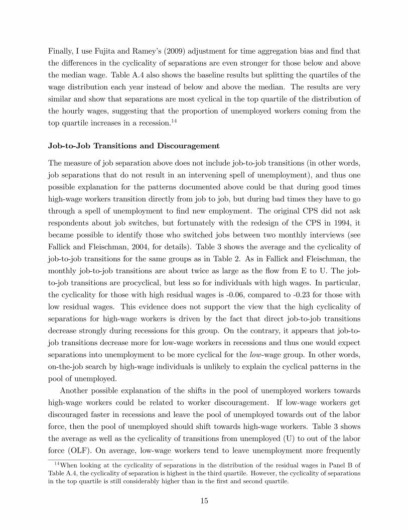
Fallick and Fleischman, 2004, for details). Table 3 shows the average and the cyclicality of

job-to-job transitions for the same groups as in Table 2. As in Fallick and Fleischman, the

monthly job-to-job transitions are about twice as large as the flow from E to U. The job-

to-job transitions are procyclical, but less so for individuals with high wages. In particular,

the cyclicality for those with high residual wages is -0.06, compared to -0.23 for those with

low residual wages. This evidence does not support the view that the high cyclicality of

separations for high-wage workers is driven by the fact that direct job-to-job transitions

decrease strongly during recessions for this group. On the contrary, it appears that job-to-

job transitions decrease more for low-wage workers in recessions and thus one would expect

separations into unemployment to be more cyclical for the low-wage group. In other words,

on-the-job search by high-wage individuals is unlikely to explain the cyclical patterns in the

pool of unemployed.

Another possible explanation of the shifts in the pool of unemployed workers towards

high-wage workers could be related to worker discouragement. If low-wage workers get

discouraged faster in recessions and leave the pool of unemployed towards out of the labor

force, then the pool of unemployed should shift towards high-wage workers. Table 3 shows

the average as well as the cyclicality of transitions from unemployed (U) to out of the labor

force (OLF). On average, low-wage workers tend to leave unemployment more frequently

14When looking at the cyclicality of separations in the distribution of the residual wages in Panel B ofTable A.4, the cyclicality of separation is highest in the third quartile. However, the cyclicality of separationsin the top quartile is still considerably higher than in the first and second quartile.

15

low high low highJob­to­job transitions Average 0.023 0.018 0.022 0.019(1994­2008 only) Cyclicality ­0.17 ­0.12 ­0.23 ­0.06

(s.e.) (0.055)*** (0.068)* (0.059)*** (0.073)

Average 0.140 0.081 0.124 0.101Cyclicality ­0.46 ­0.44 ­0.51 ­0.48(s.e.) (0.077)*** (0.173)** (0.074)*** (0.159)***

Notes: Newey­West corrected standard errors in parentheses; * significant at 10%; ** significant at 5%; ***significant at 1%. See notes in Table 1 for further details. Source: The author's estimates with data from the CPSOutgoing Rotation Group and CPS monthly files for the years 1979­2008.

Table 3. The cyclicality of job­to­job transitions and movements from unemployment (U) to out of thelabor force (OLF), by wage group

Log(hourly wage) Mincer residual

Transitions from U to OLF

towards OLF. However, the cyclicality between the two groups is almost identical, which

suggests that transitions between U and OLF cannot account for compositional changes in

the pool of unemployed documented above.

In summary, the data strongly suggests that the unemployment pool shifts towards high-

wage individuals in recessions, and this shift is mainly due to job separations.

2.4 Relation to Previous Research

Bils, Chang and Kim (2012) find similar patterns in the data for low-wage vs. high-wage

workers from the Survey of Income and Program Participation (SIPP) for the years 1983-

2003, but they focus their attention on the cyclical nature of employment for these groups

and pay little attention to the question of cyclical changes in the composition of the pool of

unemployed. More precisely, they split their sample into four groups - by low or high hours

and by low or high wages - and report the cyclicality of separations, hirings, employment

and hours worked. Averaging the cyclicality of separations for the wage groups, one finds

that the ratio of the cyclicality of separations between the low- and high-wage group is about

0.55, similar to my estimates in the CPS data.

Solon, Barsky and Parker (1994) show that there is a substantial composition bias when

looking at the cyclicality of aggregate real wages. The employed become more skilled during

recessions, leading the researcher to underestimate the cyclicality of real wages when looking

at aggregate wage data. This evidence seems to be in contrast with the facts presented above,

because it suggests that the proportion of high-wage workers among the employed increases

in recessions. However, their evidence relies on the composition bias in the aggregate hourly

wage, which is a weighted average by hours. Therefore, the composition bias could be driven

16

either by a higher cyclicality of hours for the low skilled (the intensive margin) or a higher

cyclicality of employment for the low skilled (the extensive margin). In fact, Hines, Hoynes

and Krueger (2001) show that Solon, Barsky and Parker’s results rely on the weighting of

aggregate real wages by hours worked. They demonstrate that with unweighted wage data,

composition bias has almost no effect on the cyclicality of real wages, suggesting that it is

not the composition of the employed that changes over the business cycle but rather the

hours worked by different skill groups.

Another important observation is that the pool of unemployed and the pool of employed

do not necessarily have to shift in the same direction if the pools differ in the average quality.

Specifically, since the typical unemployed is of lower ability than the typical employed, a

transition of a worker from the lower part of the distribution of the pool of employed to the

upper part of the distribution of the pool of unemployed can make both pools better off.

More formally, one can approximate the relationship between changes in the share of group i

in the pool of unemployed (dφUit) and changes in the share of group i in the pool of employed

(dφEit) as follows15:

dφEit ≈ φEit [−2UtdφUit + dU t(1− 2φUit)], (5)

which implies that if the shares of the two groups are the same (φUit = 0.5), then the pools

must sort in opposite directions. However, in reality the share of high-wage workers among

the unemployed is higher (φUhigh,t = 0.39 in the CPS sample) and thus shifts do not necessarily

go in the opposite direction. Moreover, changes in the group share among the unemployed

lead to much smaller changes in the group share among the employed, because the group

of unemployed is so much smaller compared to the group of employed. In fact, one can

compute the response of the share of the high-wage types from the estimates in Table 2, and

then use the formula in equation (5) to compute the implied change in the share in the pool

of employed. The results are as follows:

dφUhigh,tdUt

≈ 3.2

dφEhigh,tdUt

≈ 0.012,

which says that the share of the high-wage types amongh the unemployed increases by more

than three percentage points in response to a one percentage-point increase in the aggregate

unemployment rate. These results also imply that the pool of employed shifts in the same

direction, but the shift is much smaller in magnitude than for the pool of unemployed and

close to zero: A percentage-point increase in the unemployment rate increases the share of

15See Appendix B for details.

17

the high-wage types by 0.012 percentage points. To conclude, the large shifts in recessions

towards high-wage workers in the pool of unemployed documented above are consistent with

small shifts towards high-wage workers in the pool of employed.

3 Model

In this and the following section, I evaluate a number of theories that can potentially explain

the compositional shifts in the pool of unemployed over the U.S. business cycle. I start with

an extension of the standard search-matching model16 to worker heterogeneity and find

that it has diffi culties in replicating the facts summarized above. Then, I consider further

extensions of this baseline model that can potentially account for the documented facts.

In the baseline model, there are two types of workers (indexed by i) who differ in their

market productivity ai and potentially other parameters. Similar to Bils, Chang and Kim

(2012), I assume worker ability to be observable to the potential employer and thus firms

can direct their search to a particular worker type.17More precisely, there is a continuum of

workers of each type and a continuum of firms, which are matched according to the matching

function:

Mi = κuηi v1−ηi . (6)

The job finding probability is p(θi) = Mi

uiand the hiring rate q(θi) = Mi

vi.

Match productivity is defined as zxai where z is aggregate productivity, x match-specific

productivity and ai worker-specific productivity. Match-specific productivity is assumed to

follow an AR(1) process as discussed below in the calibration strategy. I assume that all

matches start at the median match productivity x̄.

Let us proceed to describe the value functions of workers and firms. The value function

of an unemployed worker of type i is:

Ui (z) = bi + βE [ (1− f(θi))Ui(z′) + f(θi)Wi(z

′, x̄)| z] , (7)

where aggregate productivity z is the aggregate state. The value of being unemployed

depends on the unemployment benefit, bi, which potentially depends on worker type, and

the discounted value of remaining unemployed in the next period or having a job with the

value Wi(z′, x̄).

16The main reference is Pissarides (2000). I deviate from his model by allowing match-specific productivityshocks to be correlated across time.17Model Appendix C1 discusses a model where worker ability is unobservable by the employer and thus

search on the firm is non-directed. The results of the model with non-directed search are similar to those ofthe model with directed search; in particular, the assumption of non-directed search has little impact on thecyclicality of separations for different ability groups.

18

The value function of an employed worker is:

Wi(z, x) = wi(z, x) + βE [max {Wi(z′, x′), Ui(z

′)}| z, x] , (8)

which depends on the utility from the current wage and the discounted future expected

value. Whenever the value of the job Wi is lower than the value of being unemployed Ui,

the worker will separate and thus receive the value Ui(z′) in the next period.

The value of posting a vacancy for a firm is:

Vi(z) = −ci + βE [ (1− q(θi))Vi(z′) + q(θi)Ji(z, x̄)| z] , (9)

which depends on the vacancy posting cost ci and the discounted future expected value.

Note that q(θi) is the firm’s hiring rate, the rate at which it fills a posted vacancy.

The value of a filled vacancy is:

Ji(z, x) = zxai − wi(z, x) + βE[

max {Ji(z′, x′), Vi(z′)}∣∣∣ z, x] , (10)

which depends on the cash flow (productivity minus the wage) and the discounted future

expected value. Note that the firm will fire the worker whenever the value of the filled

vacancy is lower than the value of posting a vacancy.

Wages are determined by standard Nash-bargaining and split the joint surplus from the

employment relationship according to the Nash-bargaining solution:

[Wi(z, x)− Ui(z)] =α

1− α [Ji(z, x)− Vi(z)] , (11)

where α is the bargaining share of the worker.

Firm-worker matches are dissolved whenever the joint surplus from the relationship

(Si(z, x) = Wi(z, x) − Ui(z) + Ji(z, x) − Vi(z)) is smaller than zero, which implies that the

reservation match productivity Ri(z), i.e., the level of match-specific productivity x below

which the employment relationship is dissolved, satisfies:

Si(z,Ri(z)) = 0. (12)

I refer to (12) as the effi cient-separation condition. Separations are always in the interest of

both parties and never unilateral (thus effi cient).

A directed search equilibrium is defined as the reservation match productivity Ri(z),

the wage schedules wi(z, x), the labor market tightness θi(z) and the value functions Ui(z),

Wi(z, x), Vi(z) and Ji(z, x) that satisfy: 1. the Nash-bargaining solution (11), 2. the effi cient-

19

separation condition (12), 3. the zero-profit condition: Vi(z) = 0 and 4. the value functions

(7), (8), (9) and (10).

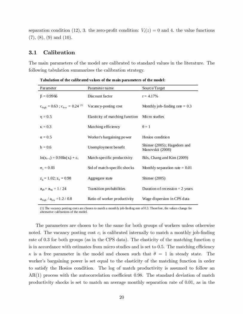
3.1 Calibration

The main parameters of the model are calibrated to standard values in the literature. The

following tabulation summarizes the calibration strategy.

Tabulation of the calibrated values of the main parameters of the model:

Parameter Parameter name Source/Target

β = 0.9966 Discount factor r = 4.17%

chigh = 0.63 ; c lo w = 0.24 (1) Vacancy­posting cost Monthly job­finding rate = 0.3

η = 0.5 Elasticity of matching function Micro studies

κ = 0.3 Matching efficiency θ = 1

α = 0.5 Worker's bargaining power Hosios condition

b = 0.6 Unemployment benefit Shimer (2005); Hagedorn andManovskii (2008)

ln(xt+1) = 0.98ln(xt) + ε t Match­specific productivity Bils, Chang and Kim (2009)

σε = 0.03 Std of match­specific shocks Monthly separation rate = 0.01

zg = 1.02; zb = 0.98 Aggregate state Shimer (2005)

πgb = πbg = 1 / 24 Transition probabilities Duration of recession = 2 years

ahigh / alow =1.2 / 0.8 Ratio of worker productivity Wage dispersion in CPS data

(1) The vacancy posting costs are chosen to match  a month ly job­finding rate of 0.3. Therefore, the values change foralternative calibrations of the model.

The parameters are chosen to be the same for both groups of workers unless otherwise

noted. The vacancy posting cost ci is calibrated internally to match a monthly job-finding

rate of 0.3 for both groups (as in the CPS data). The elasticity of the matching function η

is in accordance with estimates from micro studies and is set to 0.5. The matching effi ciency

κ is a free parameter in the model and chosen such that θ = 1 in steady state. The

worker’s bargaining power is set equal to the elasticity of the matching function in order

to satisfy the Hosios condition. The log of match productivity is assumed to follow an

AR(1) process with the autocorrelation coeffi cient 0.98. The standard deviation of match

productivity shocks is set to match an average monthly separation rate of 0.01, as in the

20

CPS data. I discretize the state space in terms of match productivities x with Tauchen’s

(1986) algorithm. Aggregate productivity z is assumed to take on two values, set to match

a standard deviation of aggregate labor productivity of 0.02, as reported by Shimer (2005).

The productivitiy parameters alow and ahigh are assumed to be 0.8 and 1.2. In the CPS

data the ratio of the wage of the group below and above the median wage is around 0.4.

Thus, the assumption of ahigh/alow = 1.2/0.8 is a conservative estimate of differences in

worker productivites. The unemployment benefit is assumed to be constant and equal to

0.6 (somewhere in between the extreme assumptions of Shimer (2005) and Hagedorn and

Manovskii (2008)). The assumption of a constant benefit by worker type implies that, at the

median match productivity x̄ = 1, the ratio of benefits over worker productivity is 0.75 for

the low types and 0.5 for the high types. This strategy is motived by two main observations:

First, wages are generally replaced only up to a specified limit. In the U.S., the maximum

unemployment benefit is binding for approximately 35% of the unemployed workers (see

Krueger and Meyer, 2002). Second, the parameter b should also capture the utility derived

from additional leisure during unemployment as well as consumption provided by additional

home production, which is likely to be less than perfectly correlated with market ability, a.

For these reasons, the replacement rates should be higher for the low-ability group.

3.2 Results

Table 4 reports results for the baseline calibration. The same filtering methods as for the

empirical results from the CPS are applied to the simulated time series. Evidently, the model

generates higher average separation rates for low-ability workers. However, the model does

not do well in capturing the cyclicality of separations as it generates a higher, not lower,

cyclicality of separations for the low-ability types.

The reason for this failure is related to the cyclical behavior of the worker’s outside

option. The effi cient-separation equation (12), rewritten for convenience, is

Wi(z, Ri(z)) + Ji(z,Ri(z)) = Ui(z),

where the left-hand side is the value of the match and the right-hand side is the value of

the outside option. When aggregate labor productivity increases, the value of the match

increases proportionally, whereas the value of being unemployed increases by less than one-

for-one because b is constant over the business cycle. Therefore, staying employed becomes

more attractive as aggregate productivity increases and thus Ri decreases. For workers with

low ability, the outside option fluctuates less as the constant term of Ui (the unemployment

benefit b) is large relative to the non-constant term (the expected value in the next period)

21

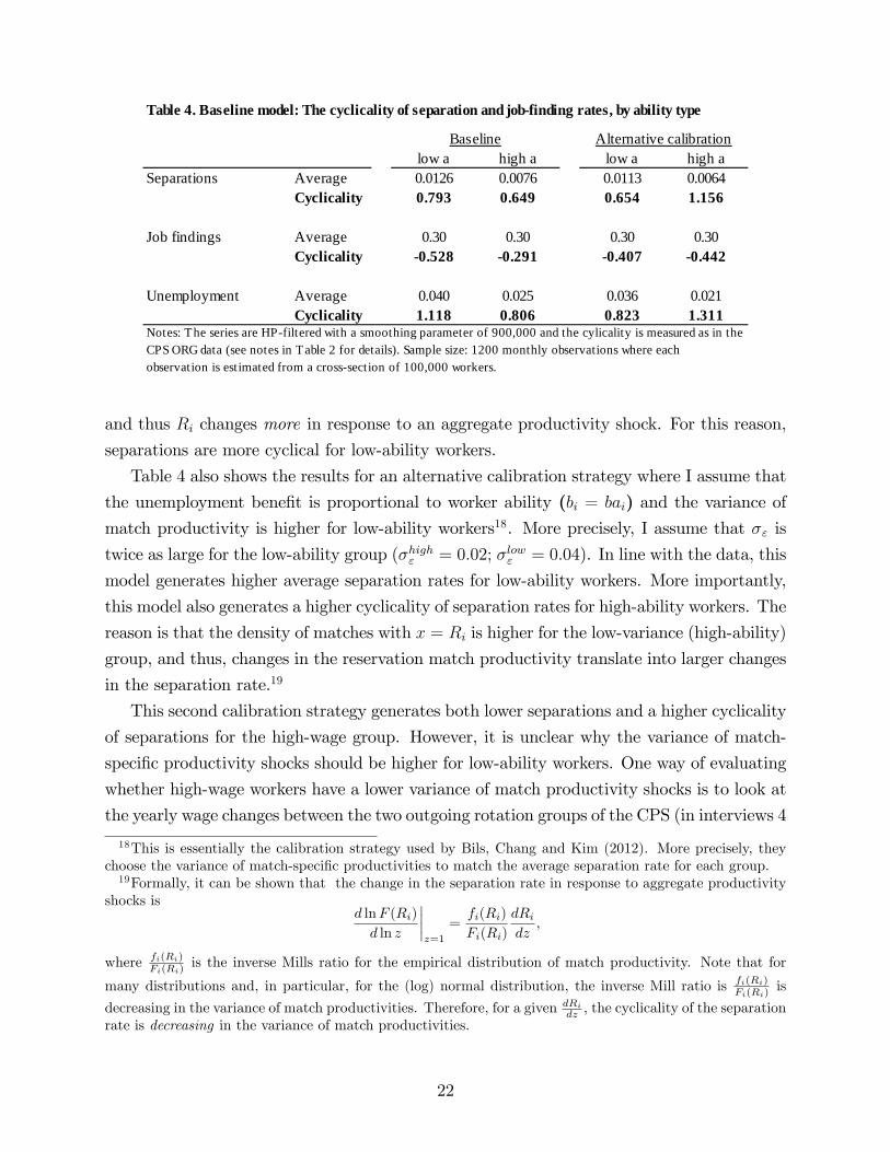
low a high a low a high aSeparations Average 0.0126 0.0076 0.0113 0.0064

Cyclicality 0.793 0.649 0.654 1.156

Job findings Average 0.30 0.30 0.30 0.30Cyclicality ­0.528 ­0.291 ­0.407 ­0.442

Unemployment Average 0.040 0.025 0.036 0.021Cyclicality 1.118 0.806 0.823 1.311

Table 4. Baseline model: The cyclicality of separation and job­finding rates, by ability type

Baseline Alternative calibration

Notes: The series are HP­filtered with a smoothing parameter of 900,000 and the cylicality is measured as in theCPS ORG data (see notes in Table 2 for details). Sample size: 1200 monthly observations where eachobservation is estimated from a cross­section of 100,000 workers.

and thus Ri changes more in response to an aggregate productivity shock. For this reason,

separations are more cyclical for low-ability workers.

Table 4 also shows the results for an alternative calibration strategy where I assume that

the unemployment benefit is proportional to worker ability (bi = bai) and the variance ofmatch productivity is higher for low-ability workers18. More precisely, I assume that σε is

twice as large for the low-ability group (σhighε = 0.02; σlowε = 0.04). In line with the data, this

model generates higher average separation rates for low-ability workers. More importantly,

this model also generates a higher cyclicality of separation rates for high-ability workers. The

reason is that the density of matches with x = Ri is higher for the low-variance (high-ability)

group, and thus, changes in the reservation match productivity translate into larger changes

in the separation rate.19

This second calibration strategy generates both lower separations and a higher cyclicality

of separations for the high-wage group. However, it is unclear why the variance of match-

specific productivity shocks should be higher for low-ability workers. One way of evaluating

whether high-wage workers have a lower variance of match productivity shocks is to look at

the yearly wage changes between the two outgoing rotation groups of the CPS (in interviews 4

18This is essentially the calibration strategy used by Bils, Chang and Kim (2012). More precisely, theychoose the variance of match-specific productivities to match the average separation rate for each group.19Formally, it can be shown that the change in the separation rate in response to aggregate productivity

shocks isd lnF (Ri)

d ln z

∣∣∣∣z=1

=fi(Ri)

Fi(Ri)

dRidz

,

where fi(Ri)Fi(Ri)

is the inverse Mills ratio for the empirical distribution of match productivity. Note that for

many distributions and, in particular, for the (log) normal distribution, the inverse Mill ratio is fi(Ri)Fi(Ri)

is

decreasing in the variance of match productivities. Therefore, for a given dRi

dz , the cyclicality of the separationrate is decreasing in the variance of match productivities.

22

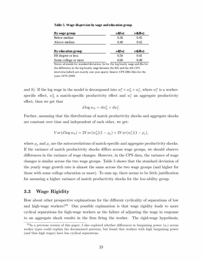
sd(lw) sd(dlw)0.36 0.450.40 0.42

sd(lw) sd(dlw)0.50 0.410.60 0.49

Notes: sd stands for standard deviation, lw for the log hourly wage and dlw forthe difference in the log hourly wage between the 8th and the 4th CPSinterview (which are exactly one year apart). Source: CPS ORG files for theyears 1979­2008.

By wage groupBelow medianAbove median

By education groupHS degree or lessSome college or more

Table 5. Wage dispersion by wage and education group

and 8). If the log wage in the model is decomposed into wai +wxit+wzt , where wai is a worker-

specific effect, wxit a match-specific productivity effect and wzt an aggregate productivity

effect, then we get that

d logwit = dwxit + dwzt .

Further, assuming that the distributions of match productivity shocks and aggregate shocks

are constant over time and independent of each other, we get:

V ar(d logwit) = 2V ar(wxit)(1− ρx) + 2V ar(wzt )(1− ρz),

where ρx and ρz are the autocorrelations of match-specific and aggregate productivity shocks.

If the variance of match productivity shocks differs across wage groups, we should observe

differences in the variance of wage changes. However, in the CPS data, the variance of wage

changes is similar across the two wage groups. Table 5 shows that the standard deviation of

the yearly wage growth rate is almost the same across the two wage groups (and higher for

those with some college education or more). To sum up, there seems to be little justification

for assuming a higher variance of match productivity shocks for the low-ability group.

3.3 Wage Rigidity

How about other prospective explanations for the different cyclicality of separations of low

and high-wage workers?20 One possible explanation is that wage rigidity leads to more

cyclical separations for high-wage workers as the failure of adjusting the wage in response

to an aggregate shock results in the firm firing the worker. The rigid-wage hypothesis,

20In a previous version of this paper, I also explored whether differences in bargaining power (αi) acrossworker types could explain the documented patterns, but found that workers with high bargaining power(and thus high wages) have less cyclical separations.

23

however, faces several diffi culties in explaining the pattern in the CPS data. First, the

wage observations in the CPS sample are 9-12 months prior to the the observed separation.

Gottschalk (2005) shows that wages are usually renegotiated one year after the last change,

which implies that for most records in my sample wages were renegotiated between interview

4 and the subsequent interviews 9-12 months later. Naturally, it is possible that wages are

renegotiated but still display substantial rigidity if the renegotiation only results in a small

wage adjustment.

Second, and more importantly, wage rigidity does not necessarily lead to more cycli-

cal separations for high-wage workers. In particular, if the contribution of match-specific

productivity shocks x to the variance of total match productivity zxai is large, it is very

diffi cult to generate a model where wage rigidity leads to more cyclical separations for high-

wage workers. If wages fail to adjust in response to match-specific productivity shocks, then

high-wage workers should also be more likely to be fired in good times. In the data, aggregate

shocks to labor productivtiy are rather small and, in particular, small compared to match-

specific shocks. In my baseline calibration above, the standard deviation of match-specific

shocks is 7.5 times higher than the standard deviation of aggregate shocks. Match-specific

shocks are not observed but inferred from wage data, and reducing the standard deviation

of match-specific productivity shocks would be at odds with data on cross-sectional wage

dispersion.

Finally, sticky wages affect separations because wages fail to adjust when they fall outside

the bargaining set (the range within which the surplus for both parties is positive). This

implies that separations may occur even if the joint surplus is positive: when wages are too

high, the firm fires the worker, whereas when wages are too low the worker quits. In both

cases, however, the parties would be better off by renegotiating the wage and thus these

separations are bilaterally ineffi cient. Another possibility would be to let wages adjust to

the boundary of the bargaining set whenever they are about to leave it. In such a model,

however, wage rigidity has little impact on separations as this type of wage rigidity affects

how the suprlus is split, but only has a limited impact on the total surplus.21 As long as

separations occur only when the total surplus is negative —i.e., as long as separations are

effi cient —the model is similar to a model with flexible wages and thus unlikely to explain

the empirical patterns of separations I have documented in the CPS data.

21Naturally, wage rigidity may have an allocative role on hiring, as emphasized in a recent literature byHall (2005), Hall and Milgrom (2008), van Rens et al. (2009) and others.

24

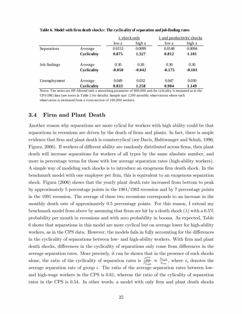
low a high a low a high aSeparations Average 0.0153 0.0099 0.0148 0.0094

Cyclicality 0.875 1.327 0.812 1.181

Job findings Average 0.30 0.30 0.30 0.30Cyclicality ­0.050 ­0.042 ­0.175 ­0.101

Unemployment Average 0.049 0.032 0.047 0.030Cyclicality 0.833 1.258 0.904 1.149

Notes: The series are HP­filtered with a smoothing parameter of 900,000 and the cylicality is measured as in theCPS ORG data (see notes in Table 2 for details). Sample size: 1200 monthly observations where eachobservation is estimated from a cross­section of 100,000 workers.

Table 6. Model with firm death shocks: The cyclicality of separation and job­finding rates

λ shock only λ and productivity shocks

3.4 Firm and Plant Death

Another reason why separations are more cylical for workers with high ability could be that

separations in recessions are driven by the death of firms and plants. In fact, there is ample

evidence that firm and plant death is countercylical (see Davis, Haltiwanger and Schuh, 1996;

Figura, 2006). If workers of different ability are randomly distributed across firms, then plant

death will increase separations for workers of all types by the same absolute number, and

more in percentage terms for those with low average separation rates (high-ability workers).

A simple way of modeling such shocks is to introduce an exogenous firm death shock. In the

benchmark model with one employee per firm, this is equivalent to an exogenous separation

shock. Figura (2006) shows that the yearly plant death rate increased from bottom to peak

by approximately 5 percentage points in the 1981/1982 recession and by 7 percentage points

in the 1991 recession. The average of these two recessions corresponds to an increase in the

monthly death rate of approximately 0.5 percentage points. For this reason, I extend my

benchmark model from above by assuming that firms are hit by a death shock (λ) with a 0.5%

probability per month in recessions and with zero probability in booms. As expected, Table

6 shows that separations in this model are more cyclical but on average lower for high-ability

workers, as in the CPS data. However, the models fails in fully accounting for the differences

in the cyclicality of separations between low- and high-ability workers. With firm and plant

death shocks, differences in the cyclicality of separations only come from differences in the

average separation rates. More precisely, it can be shown that in the presence of such shocks

alone, the ratio of the cyclicality of separation rates is βseplow

βsephigh≈ s̄high

s̄low, where s̄i denotes the

average separation rate of group i. The ratio of the average separation rates between low-

and high-wage workers in the CPS is 0.61, whereas the ratio of the cylicality of separation

rates in the CPS is 0.54. In other words, a model with only firm and plant death shocks

25

cannot fully explain the differences in cyclicality of separations in the CPS. As explained

above, productivity shocks tend to shift separations in the opposite direction and thus, they

make it even more diffi cult to fully match the differences found in the data.

4 Credit-Constraint Shocks

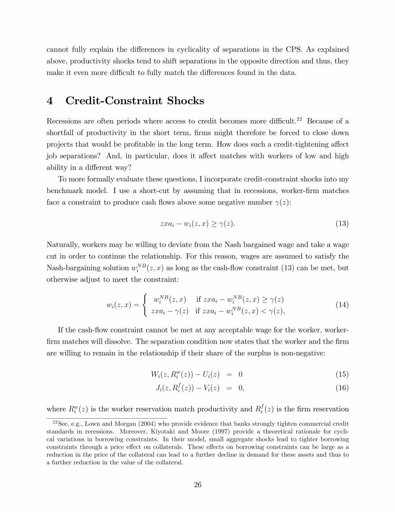
Recessions are often periods where access to credit becomes more diffi cult.22 Because of a

shortfall of productivity in the short term, firms might therefore be forced to close down

projects that would be profitable in the long term. How does such a credit-tightening affect

job separations? And, in particular, does it affect matches with workers of low and high

ability in a different way?

To more formally evaluate these questions, I incorporate credit-constraint shocks into my

benchmark model. I use a short-cut by assuming that in recessions, worker-firm matches

face a constraint to produce cash flows above some negative number γ(z):

zxai − wi(z, x) ≥ γ(z). (13)

Naturally, workers may be willing to deviate from the Nash bargained wage and take a wage

cut in order to continue the relationship. For this reason, wages are assumed to satisfy the

Nash-bargaining solution wNBi (z, x) as long as the cash-flow constraint (13) can be met, but

otherwise adjust to meet the constraint:

wi(z, x) =

{wNBi (z, x) if zxai − wNBi (z, x) ≥ γ(z)

zxai − γ(z) if zxai − wNBi (z, x) < γ(z),(14)

If the cash-flow constraint cannot be met at any acceptable wage for the worker, worker-

firm matches will dissolve. The separation condition now states that the worker and the firm

are willing to remain in the relationship if their share of the surplus is non-negative:

Wi(z, Rwi (z))− Ui(z) = 0 (15)

Ji(z,Rfi (z))− Vi(z) = 0, (16)

where Rwi (z) is the worker reservation match productivity and Rf

i (z) is the firm reservation

22See, e.g., Lown and Morgan (2004) who provide evidence that banks strongly tighten commercial creditstandards in recessions. Moreover, Kiyotaki and Moore (1997) provide a theoretical rationale for cycli-cal variations in borrowing constraints. In their model, small aggregate shocks lead to tighter borrowingconstraints through a price effect on collaterals. These effects on borrowing constraints can be large as areduction in the price of the collateral can lead to a further decline in demand for these assets and thus toa further reduction in the value of the collateral.

26

match productivity. By (15) and (16), the reservation match productivities differ between

worker and firm and separations may occur even if the joint surplus is positive.23 Actually,

firms never unilaterally fire a worker since cash-flow constraints only impose an upper limit

on the wage but not a lower limit (i.e. Rwi (z) ≥ Rf

i (z)).

If workers are willing to take wage cuts to continue the relationship, one may wonder

whether cash-flow constraints will ever result in separations. It should be kept in mind,

however, that workers are willing to take wage cuts only as long as their share of the surplus

remains positive. At the effi cient-separation level of match productivity Ri(z), for exam-

ple, workers are not willing to take any wage cut because their surplus from the match

is zero. Therefore, a binding cash-flow constraint will always lead to the separation for

the matches whose productivity is at, or below, the effi cient-separation level of match pro-

ductivity Ri(z).24 For worker-firm matches with x > Ri(z), there is some room for wage

adjustment. However, the actual wage cut that the worker may be willing to take is small,

because the surplus for those x close to Ri(z) is small.

The value functions in this model extension are the same as in the baseline model, except

for the value function of the filled vacancy:

Ji(z, x) = zxai − wi(z, x) + βE

[σwi (z′, x′) max {Ji(z′, x′), Vi(z′)}

(1− σwi (z′, x′))Vi(z′)

∣∣∣∣∣ z, x], (17)

where σwi (z′, x′) takes a value of 1 if the worker stays with the firm and 0 if the worker

quits.25

4.1 Results

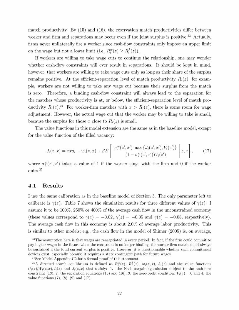
I use the same calibration as in the baseline model of Section 3. The only parameter left to

calibrate is γ(z). Table 7 shows the simulation results for three different values of γ(z). I

assume it to be 100%, 250% or 400% of the average cash flow in the unconstrained economy

(these values correspond to γ(z) = −0.02, γ(z) = −0.05 and γ(z) = −0.08, respectively).

The average cash flow in this economy is about 2.0% of average labor productivity. This

is similar to other models; e.g., the cash flow in the model of Shimer (2005) is, on average,

23The assumption here is that wages are renegotiated in every period. In fact, if the firm could commit topay higher wages in the future when the constraint is no longer binding, the worker-firm match could alwaysbe sustained if the total current surplus is positive. However, it is questionnable whether such commitmentdevices exist, especially because it requires a state contingent path for future wages.24See Model Appendix C2 for a formal proof of this statement.25A directed search equilibrium is defined as Rwi (z), R

fi (z), wi(z, x), θi(z) and the value functions

Ui(z),Wi(z, x),Vi(z) and Ji(z, x) that satisfy: 1. the Nash-bargaining solution subject to the cash-flowconstraint (13), 2. the separation equations (15) and (16), 3. the zero-profit condition: Vi(z) = 0 and 4. thevalue functions (7), (8), (9) and (17).

27

low a high a low a high a low a high aSeparations Average 0.0148 0.0094 0.0129 0.0084 0.0126 0.0078

Cyclicality 1.067 1.458 0.653 1.593 0.686 1.207

Job findings Average 0.30 0.30 0.30 0.30 0.30 0.30Cyclicality ­0.033 ­0.010 ­0.204 ­0.119 ­0.402 ­0.215

Unemployment Average 0.047 0.030 0.041 0.027 0.040 0.025Cyclicality 0.882 1.184 0.700 1.458 0.868 1.211

Table 7. Model with credit­constraint shocks: The cyclicality of separation and job­finding rates

γ = ­0.02 γ = ­0.05 γ = ­0.08

Notes: The series are HP­filtered with a smoothing parameter of 900,000 and the cylicality is measured as inthe CPS ORG data (see notes in Table 2 for details). Sample size: 1200 monthly observations where eachobservation is estimated from a cross­section of 100,000 workers.

around 1.5% of average labor productivity. It may be argued that these constraints are

very tight as a firm would need just one to four months of average productivity (depending

on the calibration of γ) to repay current losses. Note, however, that in this model, match

productivity shocks are highly correlated across time and thus, the chances of recovering

current losses are far smaller than that.

All my calibrations yield more cyclical separations for high-ability workers. The calibra-

tion with the tightest constraint (γ(z) = −0.02), however, seems unrealistic as it leads to

aggregate separations that are far too cyclical relative to aggregate job findings. The reason

is that the constraint is relatively tight, which makes aggregate separations very volatile.

The calibrations where γ(z) = −0.05 and γ(z) = −0.08 do better in that respect and, at the

same time, produce more cyclical separations for high-ability workers. Quantitatively, the

model even overpredicts the cyclicality for high-ability workers when γ(z) = −0.05, whereas

it almost exactly matches the ratio of the cyclicality of separations of low- and high-ability

workers in the CPS data when γ(z) = −0.08. It is important to point out that the re-

lationship between the tightness of the constraint in recessions and the magnitude of the

compositional shifts is non-monotonic, as the difference in the cyclicality of unemployment

rates between the two types is highest at intermediate levels of the cash flow constraint.

Therefore, testing the implications of this model extension with macro/time-series data on

firm-level financial constraints may be challenging.

4.2 Discussion

The important insight of this last model extension is that in the baseline model outlined

in Section 3, each worker-firm match produces negative cash flows at the effi cient reserva-

tion productivity level. As shown in the Model Appendix C2, the firm’s cash flows at the

28

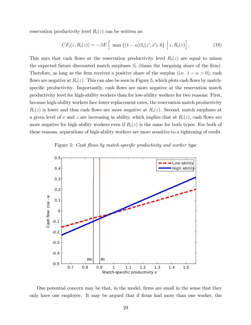
reservation productivity level Ri(z) can be written as:

CFi(z,Ri(z)) = −βE[

max {(1− α)Si(z′, x′), 0}

∣∣∣ z,Ri(z)], (18)

This says that cash flows at the reservation productivity level Ri(z) are equal to minus

the expected future discounted match surpluses Si (times the bargainig share of the firm).

Therefore, as long as the firm receives a positive share of the surplus (i.e. 1− α > 0), cash

flows are negative atRi(z). This can also be seen in Figure 5, which plots cash flows by match-

specific productivity. Importantly, cash flows are more negative at the reservation match

productivity level for high-ability workers than for low-ability workers for two reasons: First,

because high-ability workers face lower replacement rates, the reservation match productivity

Ri(z) is lower and thus cash flows are more negative at Ri(z). Second, match surpluses at

a given level of x and z are increasing in ability, which implies that at Ri(z), cash flows are

more negative for high ability workers even if Ri(z) is the same for both types. For both of

these reasons, separations of high-ability workers are more sensitive to a tightening of credit.

Figure 5: Cash flows by match-specific productivity and worker type

0.7 0.8 0.9 1 1.1 1.2 1.3 1.4 1.5­0.5

­0.4

­0.3

­0.2

­0.1

0

0.1

0.2

0.3

0.4

0.5

Rh Rl

Cas

h flo

w: z

xa ­ 

w

Match­specific productivi ty x

Low abi l ityHigh abi li ty

One potential concern may be that, in the model, firms are small in the sense that they

only have one employee. It may be argued that if firms had more than one worker, the

29

above mechanism would produce different results because the cash-flow constraint would

be operating at the firm and not at the match level. In particular, high-ability workers

generate a higher surplus for the firm (because of high expected future productivity) and

thus, the firm might prefer to lay off low-ability workers in order to keep its high-ability

workers. Notice, however, that in a multi-worker firm, each worker-firm relationship has

a shadow value of relaxing the cash-flow constraint. This shadow value is increasing more

than proportionally with the ability of the worker, because high-ability workers have lower

replacement rates and thus, in the unconstrained model, the reservation match productivity

is set to a lower level where cash flows are more negative relative to productivity. To put it

more simply, if a high-ability worker is twice as productive on average than the low-ability

type (i.e., ah = 2al), then current cash flows are more than twice as a negative at the

reservation match productivity level, and thus the multi-worker firm prefers to fire the high-

ability worker when the cash-flow constraint becomes binding. In addition, if there are small

fixed firing costs per worker, then the firm would prefer getting rid offthe high-ability worker,

even if cash flows were fully proportional to ability. For these reasons, one should expect

that - for reasonable assumptions regarding the substitutability between the two types of

workers - the main mechanisms in my model to be operative in a multi-worker firm setup.

Ideally, one should set up a multi-worker firm model to investigate the quantitative effects

of cash-flow constraints on the cyclicality of separations for low- and high-ability workers.

However, such a model is very complicated as the wage bargained by one worker affects the

firm-level cash-flow constraint and thus, the wage bargained by other workers. Stole and

Zwiebel’s (1996) intrafirm bargaining game would be a good starting point, but is further

complicated by the presence of low- and high-ability types. This important work is left for

future research.

5 Conclusion

This paper provides new facts about the composition of the unemployment pool over the

U.S. business cycle. In recessions, the pool of unemployed shifts towards workers with high

wages in their previous job. Moreover, this change is driven by the higher cyclicality of

separations for high-wage workers. These empirical patterns are diffi cult to explain with

a standard search-matching model with endogenous separations and worker heterogeneity,

since it predicts shifts in the pool of unemployed in the opposite direction of the data.

I offer two extensions of the model that work better at replicating these new facts. The

first extension introduces firm death shocks, which affect all workers indiscriminately of

type. However, these shocks cannot fully account for the more cyclical separations of high-

30

ability workers because, with such death shocks, differences in the cyclicality of separation

rates between low-wage and high-wage individuals are limited by differences in the average

separation rates between the two groups. The second extension with credit-constraint shocks,

on the other hand, can fully match the differences in the cyclicality of separations between

low- and high-ability workers. It is somewhat diffi cult to exactly pin down the magnitude of

these credit-constraint shocks, but my simulations show that the separations of high-ability

workers are more cyclical for a broad range of parameter values.

Shifts towards high-ability workers among the unemployed in slumps have important im-

plications for models of aggregate fluctuations of the labor market: if ability is not perfectly

observed to potential employers, these shifts pose an additional challenge to the recent lit-

erature on the "unemployment volatility puzzle" (see Shimer, 2005). More precisely, these

compositional changes aggravate the apparent lack of an amplification mechanism in the

standard search-matching model, as they dampen the response of the firms’recruiting be-

havior to aggregate productivity shocks. Moreover, the shifts may have a large impact on the

welfare costs of business cycles as high-ability workers are better able to self-insure against

unemployment shocks (see, e.g., Mukoyama and Sahin, 2006). To conduct a proper welfare

analysis, however, I have to model the savings and consumption choices of the employed and

unemployed. I leave this important task to future research.

Another avenue for future research is to extend my empirical analysis with other data

sources. Matched employer-employee data is particularly promising as it allows us to deter-

mine the importance of firm death for separations. Moreover, it makes it possible to extract

individual fixed effects from the wage and perform the same type of analysis with the av-

erage individual effect instead of the average previous wage. It will also be interesting to

extend my empirical analysis to other countries. Many European countries have an extensive

employment protection legislation, which may affect the sign as well as the magnitude of

the shifts in the unemployment pool. E.g., seniority rules make it harder for firms to lay

off more experienced workers. But it is unclear how these rules interact with the business

cycle, as they may be circumvented or inapplicable in recessions (e.g., because of firm and

plant death).26 Finally, matched employer-employee data could also be used to test for the

importance of credit frictions for the compositional changes in the pool of unemployed, if

balance sheet information on the firm side is obtained.

26Forslund et al. (2011) provide some evidence for Sweden that suggests similar patterns as in the U.S.

31

References

[1] Abowd, J., Zellner, A. (1985). "Estimating Gross Labor-Force Flows," Journal of Busi-

ness & Economic Statistics 3(3), 254-83.

[2] Bils, M. (1985). “Real Wages over the Business Cycle: Evidence from Panel Data,”

Journal of Political Economy 93(4), 666-89.

[3] Bils, M., Chang, Y., Kim, S.-B. (2009). "Comparative Advantage and Unemployment,"

RCER Working Papers 547, University of Rochester.

[4] Bils, M., Chang, Y., Kim, S.-B. (2012). "Comparative Advantage and Unemployment,"

Journal of Monetary Economics 59(2), pp. 150-165.

[5] Bleakley, H., Ferris, A., Fuhrer, J. (1999). "New Data on Worker Flows During Business

Cycles," New England Economic Review, issue Jul, 49-76.

[6] Davis, S., Haltiwanger, J. and Schuh, S. (1996). Job Creation and Destruction, Cam-

bridge: MIT Press.

[7] Elsby, M., Michaels, R., Solon, G. (2009). "The Ins and Outs of Cyclical Unemploy-

ment," American Economic Journal: Macroeconomics 1(1), 84-110.

[8] Fallick, B., Fleischman, Ch. (2004). "Employer-to-Employer Flows in the U.S. Labor

Market: The Complete Picture of Gross Worker Flows," Finance and Economics Dis-

cussion Series 2004-34, Board of Governors of the Federal Reserve System.

[9] Figura, A. (2006). "Why are Plant Deaths Countercyclical: Reallocation Timing or

Fragility?," Finance and Economics Discussion Series 2006-31, Board of Governors of

the Federal Reserve System.

[10] Forslund, A., Fredriksson, P., Vikström, J. (2011). "What active labor market policy

works best in a recession?" IFAU working paper 2011:2.

[11] Fujita, S., Ramey, G. (2009). "The Cyclicality Of Separation And Job Finding Rates,"

International Economic Review 50(2), pp. 415-430.

[12] Gottschalk, P. (2005). "Downward Nominal-Wage Flexibility: Real or Measurement

Error?," The Review of Economics and Statistics 87(3), 556-68.

[13] Haefke, Ch., Sonntag, M., van Rens, Th. (2012). "Wage Rigidity and Job Creation,"

CEPR Discussion Paper 8968.

32

[14] Hagedorn, M., Manovskii, I. (2008). "The Cyclical Behavior of Equilibrium Unemploy-

ment and Vacancies Revisited," American Economic Review 98(4), 1692-1706.

[15] Hall, R. (2005), “Employment Fluctuations with Equilibrium Wage Stickiness”, Amer-

ican Economic Review 95(1), 50- 65.

[16] Hall, R., Milgrom, P. (2008). "The Limited Influence of Unemployment on the Wage

Bargain," American Economic Review, 98(4), 1653-74.

[17] Hines, J., Hoynes, H., Krueger, A. (2001). "Another Look at Whether a Rising Tide

Lifts All Boats" In: Alan B. Krueger and Robert Solow (editors), The Roaring Nineties:

Can Full Employment Be Sustained? New York: Russell Sage Foundation.

[18] Kiyotaki, N., Moore, J. (1997). "Credit Cycles," Journal of Political Economy 105(2),

211-48.

[19] Krueger, A., Meyer, B. (2002). “Labor Supply Effects of Social Insurance.” In: Alan

Auerbach and Martin Feldstein (editors), Handbook of Public Economics Vol 4. North-

Holland: Amsterdam.

[20] Krusell, P., Smith, A. (1998). "Income andWealth Heterogeneity in the Macroeconomy,"

Journal of Political Economy 106(5), 867-896.

[21] Lown, C., Morgan, D. (2006). "The Credit Cycle and the Business Cycle: New Findings

Using the Loan Offi cer Opinion Survey," Journal of Money, Credit and Banking 38(6),

1575-1597.

[22] Madrian, B., Lefgren, L. (1999). "A Note on Longitudinally Matching Current Popula-

tion Survey (CPS) Respondents," NBER Technical Working Papers 0247.

[23] Mukoyama, T., Sahin, A. (2006). "Costs of Business Cycles for Unskilled Workers,"

Journal of Monetary Economics 53(8), 2179-2193.

[24] Pissarides, C. (2000). Equilibrium Unemployment Theory, MIT Press, Cambridge, MA.

[25] Pries, M. (2008). “Worker Heterogeneity and Labor Market Volatility in Matching Mod-

els,”Review of Economic Dynamics 11(3), 664-678.

[26] Shimer, R. (2005). “The Cyclical Behavior of Equilibrium Unemployment and Vacan-

cies,”American Economic Review 95(1), 25-49.

[27] Shimer, R. (2007). "Reassessing the Ins and Outs of Unemployment," NBER Working

Papers 13421.

33

[28] Solon, G., Barsky, R., Parker, J. (1994). “Measuring the Cyclicality of Real Wages:

How Important Is Composition Bias?,”Quarterly Journal of Economics 109(1), 1-25.

[29] Stole, L., Zwiebel, J. (1996). "Organizational Design and Technology Choice under

Intrafirm Bargaining," American Economic Review 86(1), 195-222.

[30] Tauchen, G. (1986). “Finite State Markov-Chain Approximations to Univariate and

Vector Autoregressions”, Economics Letters 20, 177-181.

34

Appendix

A1. CPS Outgoing Rotation Group and monthly files (1979-2008)

A1.1 Hourly wage series

I use the CPS ORG files provided by the Center for Economic and Policy Research (CEPR).

These files are based on the NBER version of the CPS ORG files, and include additional

wage series that adjust the NBER series of the hourly wage for overtime earnings, tips and

commissions, and impute earnings above the top code. Earnings above the top code are

imputed based on assuming a distribution of wages, and I choose the variable w_ln_ot,

which assumes a logarithmic distribution of earnings. As Haefke et al. (2012), I deflate

nominal hourly wages with the implicit deflator for hourly earnings in the private non-farm

business sector from the BLS productivity and costs program. To address potential issues

related to outliers, I drop all wage observations below the 0.25th and above the 99.75th

percentile in each year, as well as drop individuals who work less than 5 hours or more than

80 hours.

A1.2 Matching

Due to moves into and out of household addresses, invalid matches must be eliminated based

on demographic information. I use the s|r|a criterion of Madrian and Lefgren (1999), becauseit appears to yield a relatively good trade-offbetween accepting invalid matches and rejecting

valid matches. The criterion keeps as valid matches only those observations with the same

sex, race and an age difference of 0-2 years.

To match the different interviews, I proceed in two steps: First, I match the eighth

interview from the CPS ORG data to the fourth interview in the CPS ORG data and then,

second, I match the additional monthly interviews 5, 6 and 7 to the fourth interview.

A1.3 Industry and occupation codes

At the 2-digit level, the NBER created industry that are consistent across all years. At

the 3-digit level, the occupation and industry classification in the CPS ORG files changed

coding scheemes in 1983, 1992 and 2003. I use the variables occ1950 and ind1950 from

the IPUMS-CPS, which is a harmonized 3-digit occupation and industry scheeme across all

years.

A1.4 Mincerian wage regressions

In part of the analysis in Section 2, I use wage residuals. The regression I run to create these

residuals, is the log hourly wage on potential expericence (quadratic polynomial), educational

attainment, gender, marital status, an interaction term between marital status and gender,

dummies for black, hispanic and other race and dummies for each state, year, occupation

and industry. Potential experience is defined as age minus years of school and minus 6. In

order to take into account for changes in the coeffi cients of the regression over time, I run

the regression for each year in a rolling window (i.e., including data from plus and minus

five years) and then compute the residual for that year.

A2. CPS March files (1962-2011)

I use the CPS-IPUMS version of the CPS March supplement. As mentioned in the main

text, the CPS March supplement does not contain a measure of hours worked on the previous

job for the period prior to 1976. For this reason, I use the weekly wage. The weekly wage

is derived from the variable of total wage and salary income during the previous calendar

year and then divided by the number of weeks worked during the previous calendar year.

For the period prior to 1976 the measure of weeks worked is only available as a categorical

variable, and I impute the weeks worked by the midpoint of each interval from data for

the period 1976 and onwards (the intervals are 1-13 weeks, 14-26 weeks, 27-39 weeks, 40-47

weeks, 48-49 weeks and 50-52 weeks). As in the CPS ORG and monthly data, I deflate

nominal hourly wages with the implicit deflator for hourly earnings in the private non-farm

business sector from the BLS productivity and costs program, and drop all wage observations

below the 0.25th and above the 99.75th percentile in each year. I use the same industry and

occupation classification scheme and run the same wage regressions as in the analysis with

the CPS ORG and monthly data.

B. The relationship between changes in the composition of the un-

employed and changes in the composition of the employed

Let’s divide the pool of employed in two equally large group, i.e., into those below and above

the median. The share of unemployed and the share of employed of group i then can be

written as:

φUit = ψiUitUt

(19)

φEit = ψiEitEt

(20)

where i stands for low or high, and where ψiis the population share of group i. The changes

in the shares then can be written as

dφUit = φUit [d lnUit − d lnUt]

dφEit = φEit [d lnEit − d lnEt]

= φEit [d ln(1− Uit)− d ln(1− Ut)]

and where the latter can be approximated as

dφEit ≈ φEit [dUt − dUit]≈ φEit [Utd lnUt − Uitd lnUit]

≈ φEit

[Utd lnUt −

Uit

φUit

(dφUit + φUitd lnUt

)]≈ φEitUt

[− 1

ψi

(dφUit

)+

(Ut − Uit)Ut

d lnUt

]≈ φEit

[−2Ut

(dφUit

)+(1− 2φUit

)dUt]

and using the averages and the cyclicality of unemployment by wage group from Table 2, we

get:

dφUhigh,tdUt

=φUhigh,tUt

[d lnUhigh,td lnUt

− 1

]=

0.39

0.0305(1.25− 1)

= 3.2

dφEhigh,tdUt

≈ φEhigh,t

[−2Ut

(dφUhigh,tdUt

)+(1− 2φUhigh,t

)]≈ 0.5 [−2(0.0305) (3.2) + (1− 2(0.39))]

≈ 0.012

where Ut =Ulow,t+Uhigh,t

2= 0.0305, where φUhigh,t = ψhigh

Uhigh,tUt

= 0.5 0.0240.0305

= 0.39 and where I

have assumed that φEhigh,t = ψiEitEt

= 0.5EitEt≈ 0.5 at all times.

C1. A Search-Matching Model with Non-Directed Search

If search on the firm side is non-directed to a particular worker type, then there is only one

aggregate matching function:

M = κuηv1−η. (21)

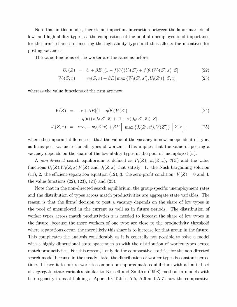
Note that in this model, there is an important interaction between the labor markets of

low- and high-ability types, as the composition of the pool of unemployed is of importance

for the firm’s chances of meeting the high-ability types and thus affects the incentives for

posting vacancies.

The value functions of the worker are the same as before:

Ui (Z) = bi + βE [ (1− f(θi))Ui(Z′) + f(θi)Wi(Z

′, x̄)|Z] (22)

Wi(Z, x) = wi(Z, x) + βE [max {Wi(Z′, x′), Ui(Z

′)}|Z, x] , (23)

whereas the value functions of the firm are now:

V (Z) = −c+ βE[(1− q(θ))V (Z ′) (24)

+ q(θ) (πJl(Z′, x̄) + (1− π)Jh(Z

′, x̄))|Z]

Ji(Z, x) = zxai − wi(Z, x) + βE[

max {Ji(Z ′, x′), V (Z ′)}∣∣∣Z, x] , (25)

where the imporant difference is that the value of the vacancy is now independent of type,

as firms post vacancies for all types of workers. This implies that the value of posting a

vacancy depends on the share of the low-ability types in the pool of unemployed (π).

A non-directed search equilibrium is defined as Ri(Z), wi(Z, x), θ(Z) and the value

functions Ui(Z),Wi(Z, x),V (Z) and Ji(Z, x) that satisfy: 1. the Nash-bargaining solution

(11), 2. the effi cient-separation equation (12), 3. the zero-profit condition: V (Z) = 0 and 4.

the value functions (22), (23), (24) and (25).

Note that in the non-directed search equilibrium, the group-specific unemployment rates

and the distribution of types across match productivities are aggregate state variables. The

reason is that the firms’decision to post a vacancy depends on the share of low types in

the pool of unemployed in the current as well as in future periods. The distribution of

worker types across match productivties x is needed to forecast the share of low types in

the future, because the more workers of one type are close to the productivity threshold

where separations occur, the more likely this share is to increase for that group in the future.

This complicates the analysis considerably as it is generally not possible to solve a model

with a highly dimensional state space such as with the distribution of worker types across

match productivties. For this reason, I only do the comparative statitics for the non-directed

search model because in the steady state, the distribution of worker types is constant across

time. I leave it to future work to compute an approximate equilibrium with a limited set

of aggregate state variables similar to Krusell and Smith’s (1998) method in models with

heterogeneity in asset holdings. Appendix Tables A.5, A.6 and A.7 show the comparative

statics results for the directed and non-directed search model. The results between the two

models are similar; in particular, the differences in the cyclicality of separations between

the low- and high-ability types are not affected to any considerable extent by the modeling

choices on non-directed or directed search.

C2. A Search-Matching Model with Cash-Flow Constraints

This appendix provides formal propositions and proofs of the intuition explained in the text.

Proposition 1 At the effi cient reservation match productivity Ri(z), the firm’s cash flows

are negative if the firm’s bargaining share is larger than 0.

Proof. At Ri(z), the joint surplus of the match is zero, as well as the surplus share of the

firm. Because of the zero-profit condition, we get:

0 = Ji(z,R(z))− Vi(z)

= Ji(z,R(z))

= CFi(z,R(z)) + βE[

max {Ji(z′, x′), 0}∣∣∣ z,Ri(z)

],

and thus

CFi(z,Ri(z)) = −βE[

max {Ji(z′, x′), 0}∣∣∣ z,Ri(z)

]= −βE

[max {(1− α)Si(z

′, x′), 0}∣∣∣ z, Ri(z)

],

which says that cash flows have to be negative at the effi cient reservation match productivity

level if the firm expects a surplus from the match in the future, i.e., if the firm’s surplus

share is positive (1 − α > 0). This holds for any process of match productivity with some

positive probability of a higher match productivity in future periods.

Proposition 2 At the effi cient reservation match productivity Ri(z), wages do not adjust

in response to a credit-constraint shock, and matches separate if the constraint is binding.

Proof. At the effi cient reservation match productivity, the total match surplus as well asthe worker share of the surplus is zero. Therefore, the worker is not willing to take a wage

cut, because it would result in a negative surplus share for the worker.

Proposition 3 If bi = bai and f(θi) = f , then, at the effi cient reservation match produc-

tivity Ri(z), cash flows are more negative for high-ability workers.

Proof. From the proposition above, we know that the cash flow at the reservation match

productivity level depends on the discounted future expected surplus. So if the expected

surplus is higher for high-ability workers, then cash flows are more negative at Ri(z). If

bi = bai, then the surplus can be written as:

Si(z, x) = Wi(z, x)− Ui(z) + Ji(z, x)

= ai(zx− b) + βE [max {Si(z′, x′), 0}| z, x]

−βf(θi)αE [max {Si(z′, x̄), 0}| z] ,

and if f(θi) = f(θ), then

Si(z, x) = aiS̃(z, x),

where S̃(z, x) ≥ 0 is independent of ability. This implies that the surplus is increasing

proportionally to ability and thus cash flows at Ri(z) are more negative for high-ability

workers.

It follows that if dbidai

= 0, cash flows at the reservation match productivity level are

even more negative for high-ability workers, since the surplus is even higher for high-ability

workers. Note that the assumption that the job-finding rates are the same for the two groups

is not necessarily met: the model calibration targets the average job-finding rate to be 0.3

for both groups, but the job-finding rates are allowed to differ over the cycle.

Appendix Tables

low high low highFull sample (Baseline) Cyclicality 0.40 0.74 0.43 0.68

(s.e.) (0.078)*** (0.096)*** (0.063)*** (0.077)***

Cyclicality 0.05 0.30 0.07 0.24(s.e.) (0.043) (0.054)*** (0.046) (0.054)***

Subsample: not on temporary layoff Cyclicality 0.40 0.73 0.38 0.75(1988­2008 only) (s.e.) (0.087)*** (0.141)*** (0.107)*** (0.097)***

Subsample: age 25­54 Cyclicality 0.42 0.75 0.44 0.73(s.e.) (0.083)*** (0.077)*** (0.071)*** (0.073)***

Subsample: men Cyclicality 0.45 0.73 0.49 0.72(s.e.) (0.076)*** (0.081)*** (0.064)*** (0.083)***

Subsample: full­time workers Cyclicality 0.37 0.73 0.41 0.68(s.e.) (0.083)*** (0.098)*** (0.067)*** (0.080)***

Subsample: some college or more Cyclicality 0.42 0.72 0.45 0.75(s.e.) (0.119)*** (0.108)*** (0.103)*** (0.091)***

Cyclicality 0.43 0.73 0.43 0.70(s.e.) (0.067)*** (0.137)*** (0.059)*** (0.099)***

Cyclicality 0.54 1.06 0.62 0.98(s.e.) (0.163)*** (0.167)*** (0.109)*** (0.161)***

Cyclicality 0.39 0.76 0.42 0.69(s.e.) (0.055)*** (0.064)*** (0.051)*** (0.061)***

Cyclicality 0.29 0.60 0.30 0.55(s.e.) (0.080)*** (0.104)*** (0.067)*** (0.082)***

Table A.1 The cyclicality of separation rates, by wage group (robustness checks)

Log(hourly wage) Mincer residual

Notes: Newey­West corrected standard errors in parentheses; * significant at 10%; ** significant at 5%; ***significant at 1%. All series are HP­filtered with a smoothing parameter of 900,000 (unless otherwise stated). Thecylicality is measured as the coefficient β in the regression log(xit) = α+βlog(Ut)+εit , where xit  is the separation,job­finding or unemployment rate of group i at t ime t and Ut is the sample unemployment rate. Similar to Bils,Chang and Kim (2009), I instrument the sample unemployment rate with the official unemployment rate becauseof measurement error. Sample size: 322 monthly observations. Source: The author's estimates with data from theCPS Outgoing Rotation Group and CPS monthly files for the years 1979­2008.

Adjusted for time aggregation bias

Filtering: HP­filtered with smoothingparameter 14400

Filtering: Not filtered, but controllingfor linear trend

Subsample: not manufacturing andnot construction

Extended sample: Unemployed ANDout of the labor force

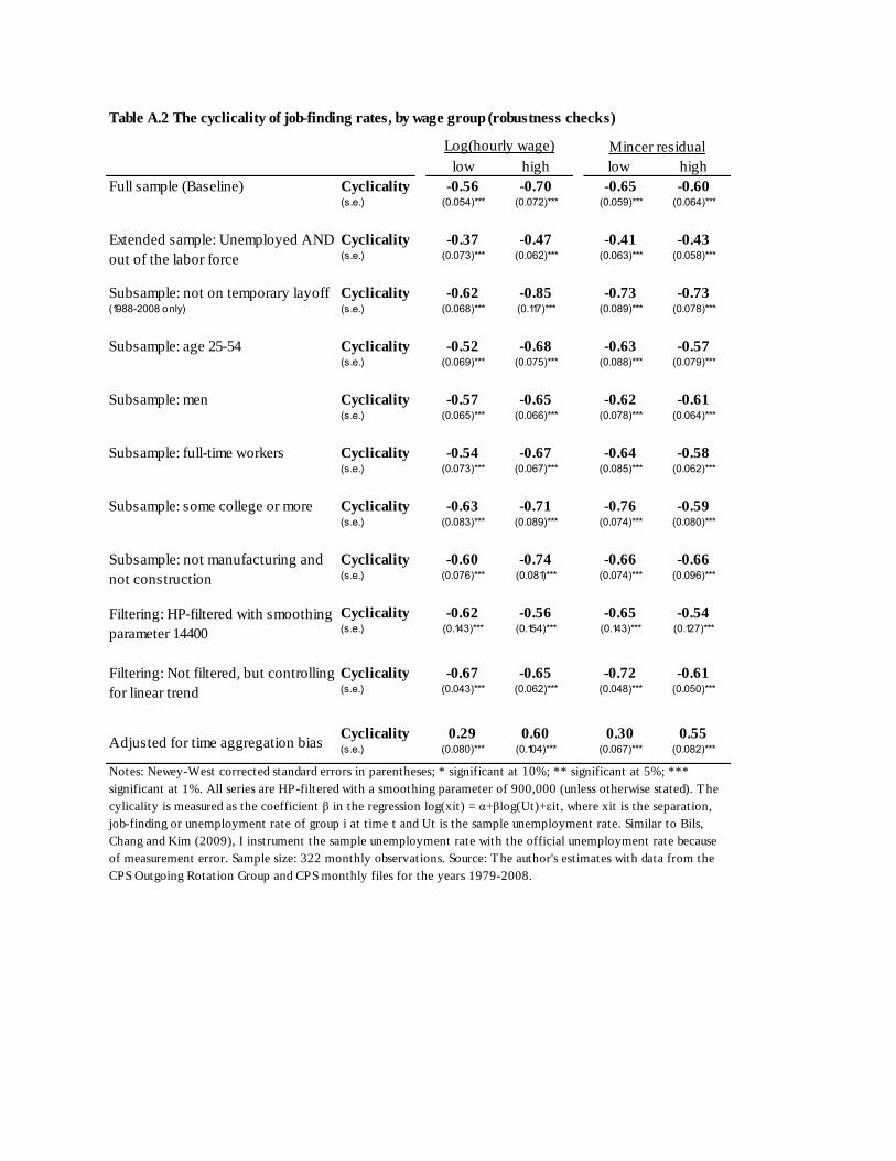
low high low highFull sample (Baseline) Cyclicality ­0.56 ­0.70 ­0.65 ­0.60

(s.e.) (0.054)*** (0.072)*** (0.059)*** (0.064)***

Cyclicality ­0.37 ­0.47 ­0.41 ­0.43(s.e.) (0.073)*** (0.062)*** (0.063)*** (0.058)***

Subsample: not on temporary layoff Cyclicality ­0.62 ­0.85 ­0.73 ­0.73(1988­2008 only) (s.e.) (0.068)*** (0.117)*** (0.089)*** (0.078)***

Subsample: age 25­54 Cyclicality ­0.52 ­0.68 ­0.63 ­0.57(s.e.) (0.069)*** (0.075)*** (0.088)*** (0.079)***

Subsample: men Cyclicality ­0.57 ­0.65 ­0.62 ­0.61(s.e.) (0.065)*** (0.066)*** (0.078)*** (0.064)***

Subsample: full­time workers Cyclicality ­0.54 ­0.67 ­0.64 ­0.58(s.e.) (0.073)*** (0.067)*** (0.085)*** (0.062)***

Subsample: some college or more Cyclicality ­0.63 ­0.71 ­0.76 ­0.59(s.e.) (0.083)*** (0.089)*** (0.074)*** (0.080)***

Cyclicality ­0.60 ­0.74 ­0.66 ­0.66(s.e.) (0.076)*** (0.081)*** (0.074)*** (0.096)***

Cyclicality ­0.62 ­0.56 ­0.65 ­0.54(s.e.) (0.143)*** (0.154)*** (0.143)*** (0.127)***

Cyclicality ­0.67 ­0.65 ­0.72 ­0.61(s.e.) (0.043)*** (0.062)*** (0.048)*** (0.050)***

Cyclicality 0.29 0.60 0.30 0.55(s.e.) (0.080)*** (0.104)*** (0.067)*** (0.082)***

Notes: Newey­West corrected standard errors in parentheses; * significant at 10%; ** significant at 5%; ***significant at 1%. All series are HP­filtered with a smoothing parameter of 900,000 (unless otherwise stated). Thecylicality is measured as the coefficient β in the regression log(xit) = α+βlog(Ut)+εit , where xit  is the separation,job­finding or unemployment rate of group i at t ime t and Ut is the sample unemployment rate. Similar to Bils,Chang and Kim (2009), I instrument the sample unemployment rate with the official unemployment rate becauseof measurement error. Sample size: 322 monthly observations. Source: The author's estimates with data from theCPS Outgoing Rotation Group and CPS monthly files for the years 1979­2008.

Adjusted for time aggregation bias

Filtering: HP­filtered with smoothingparameter 14400

Filtering: Not filtered, but controllingfor linear trend

Table A.2 The cyclicality of job­finding rates, by wage group (robustness checks)

Log(hourly wage) Mincer residual

Subsample: not manufacturing andnot construction

Extended sample: Unemployed ANDout of the labor force

low high low highFull sample (Baseline) Cyclicality 0.81 1.25 0.89 1.13

(s.e.) (0.024)*** (0.030)*** (0.025)*** (0.031)***

Cyclicality 0.20 0.53 0.24 0.41(s.e.) (0.022)*** (0.037)*** (0.020)*** (0.033)***

Subsample: not on temporary layoff Cyclicality 0.81 1.34 0.90 1.20(1988­2008 only) (s.e.) (0.049)*** (0.069)*** (0.053)*** (0.056)***

Subsample: age 25­54 Cyclicality 0.80 1.23 0.89 1.13(s.e.) (0.022)*** (0.026)*** (0.028)*** (0.034)***

Subsample: men Cyclicality 0.79 1.18 0.86 1.16(s.e.) (0.033)*** (0.027)*** (0.029)*** (0.033)***

Subsample: full­time workers Cyclicality 0.80 1.21 0.89 1.11(s.e.) (0.027)*** (0.028)*** (0.026)*** (0.028)***

Subsample: some college or more Cyclicality 0.82 1.15 0.95 1.06(s.e.) (0.046)*** (0.037)*** (0.033)*** (0.040)***

Cyclicality 0.82 1.26 0.87 1.15(s.e.) (0.025)*** (0.036)*** (0.029)*** (0.037)***

Cyclicality 0.81 1.22 0.86 1.16(s.e.) (0.050)*** (0.063)*** (0.051)*** (0.065)***

Cyclicality 0.84 1.22 0.89 1.13(s.e.) (0.023)*** (0.030)*** (0.023)*** (0.028)***

Notes: Newey­West corrected standard errors in parentheses; * significant at 10%; ** significant at 5%; ***significant at 1%. All series are HP­filtered with a smoothing parameter of 900,000 (unless otherwise stated). Thecylicality is measured as the coefficient β in the regression log(xit) = α+βlog(Ut)+εit , where xit  is the separation,job­finding or unemployment rate of group i at t ime t and Ut is the sample unemployment rate. Similar to Bils,Chang and Kim (2009), I instrument the sample unemployment rate with the official unemployment rate becauseof measurement error. Sample size: 322 monthly observations. Source: The author's estimates with data from theCPS Outgoing Rotation Group and CPS monthly files for the years 1979­2008.

Filtering: HP­filtered with smoothingparameter 14400

Filtering: Not filtered, but controllingfor linear trend

Table A.3 The cyclicality of unemployment rates, by wage group (robustness checks)

Log(hourly wage) Mincer residual

Subsample: not manufacturing andnot construction

Extended sample: Unemployed ANDout of the labor force

1st 2nd 3rd 4thSeparations Cyclicality 0.29 0.55 0.68 0.82

(s.e.) (0.117)** (0.085)*** (0.109)*** (0.128)***

Job findings Cyclicality ­0.49 ­0.63 ­0.66 ­0.69(s.e.) (0.058)*** (0.079)*** (0.078)*** (0.093)***

Unemployment Cyclicality 0.67 0.99 1.24 1.27(s.e.) (0.044)*** (0.035)*** (0.061)*** (0.058)***

1st 2nd 3rd 4thSeparations Cyclicality 0.39 0.47 0.74 0.65

(s.e.) (0.100)*** (0.083)*** (0.092)*** (0.106)***

Job findings Cyclicality ­0.66 ­0.63 ­0.62 ­0.56(s.e.) (0.068)*** (0.120)*** (0.128)*** (0.103)***

Unemployment Cyclicality 0.86 0.92 1.17 1.11(s.e.) (0.037)*** (0.052)*** (0.036)*** (0.062)***

Notes: Newey­West corrected standard errors in parentheses; * significant at  10%; ** significant at  5%;*** significant at 1%. All series are HP­filtered with a smoothing parameter of 900,000. The cylicality ismeasured as the coefficient  β in the regression log(xit) = α+βlog(Ut)+εit , where xit  is the separation, hiringor unemployment rate of group i at t ime t and Ut is the sample unemployment rate. Similar to Bils, Changand Kim (2009), I instrument the sample unemployment rate with the official unemployment rate becauseof measurement error. Sample size: 322 monthly observations. Source: The author's estimates with datafrom the CPS Outgoing Rotation Group and CPS monthly files for the years 1979­2008.

Table A.4 The cyclicality of separation and job­finding rates, by wage group (quartiles)

Panel A. Log(hourly wage)

Panel B. Mincer­residual

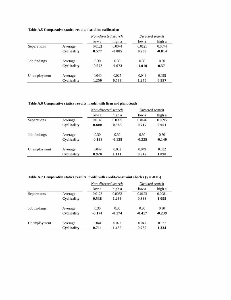
low a high a low a high aSeparations Average 0.0121 0.0074 0.0121 0.0074

Cyclicality 0.577 ­0.085 0.260 ­0.014

Job findings Average 0.30 0.30 0.30 0.30Cyclicality ­0.673 ­0.673 ­1.010 ­0.571

Unemployment Average 0.040 0.025 0.041 0.025Cyclicality 1.250 0.588 1.270 0.557

low a high a low a high aSeparations Average 0.0146 0.0095 0.0146 0.0095

Cyclicality 0.800 0.983 0.717 0.951

Job findings Average 0.30 0.30 0.30 0.30Cyclicality ­0.128 ­0.128 ­0.225 ­0.140

Unemployment Average 0.049 0.032 0.049 0.032Cyclicality 0.928 1.111 0.942 1.090

low a high a low a high aSeparations Average 0.0123 0.0082 0.0123 0.0081

Cyclicality 0.538 1.266 0.363 1.095

Job findings Average 0.30 0.30 0.30 0.30Cyclicality ­0.174 ­0.174 ­0.417 ­0.239

Unemployment Average 0.041 0.027 0.041 0.027Cyclicality 0.711 1.439 0.780 1.334

Non­directed search Directed search

Non­directed search Directed search

Table A.6 Comparative statics results: model with firm and plant death

Table A.7 Comparative statics results: model with credit­constraint shocks (γ = ­0.05)

Table A.5 Comparative statics results: baseline calibration

Non­directed search Directed search