discriminative, generative and imitative learningjebara/papers/jebara4.pdf · discriminative,...
TRANSCRIPT

Discriminative, Generative and ImitativeLearning
byTony Jebara
B.Eng., Electrical Engineering McGill University, 1996M.Sc., Media Arts and Sciences, MIT, 1998
Submitted to the Program in Media Arts and Sciences,School of Architecture and Planning,
in partial fulfillment of the requirements for the degree ofDOCTOR OF PHILOSOPHY IN MEDIA ARTS AND SCIENCES
at theMassachusetts Institute of Technology
February 2002
c©Massachusetts Institute of Technology, 2002All Rights Reserved
Signature of Author
Program in Media Arts and SciencesDecember 18, 2001
Certified by
Alex P. PentlandToshiba Professor of Media Arts and Sciences
Program in Media Arts and SciencesThesis Supervisor
Accepted by
Andrew B. LippmanChair
Departmental Committee on Graduate StudentsProgram in Media Arts and Sciences

Discriminative, Generative and Imitative Learning
byTony Jebara
Submitted to the Program in Media Arts and Sciences,School of Architecture and Planning,
in partial fulfillment of the requirements for the degree of
Doctor of Philosophy in Media Arts and Sciences
Abstract
I propose a common framework that combines three different paradigms in machine learning: gen-erative, discriminative and imitative learning. A generative probabilistic distribution is a principledway to model many machine learning and machine perception problems. Therein, one provides do-main specific knowledge in terms of structure and parameter priors over the joint space of variables.Bayesian networks and Bayesian statistics provide a rich and flexible language for specifying thisknowledge and subsequently refining it with data and observations. The final result is a distributionthat is a good generator of novel exemplars.
Conversely, discriminative algorithms adjust a possibly non-distributional model to data optimizingfor a specific task, such as classification or prediction. This typically leads to superior performanceyet compromises the flexibility of generative modeling. I present Maximum Entropy Discrimination(MED) as a framework to combine both discriminative estimation and generative probability den-sities. Calculations involve distributions over parameters, margins, and priors and are provably anduniquely solvable for the exponential family. Extensions include regression, feature selection, andtransduction. SVMs are also naturally subsumed and can be augmented with, for example, featureselection, to obtain substantial improvements.
To extend to mixtures of exponential families, I derive a discriminative variant of the Expectation-Maximization (EM) algorithm for latent discriminative learning (or latent MED). While EM andJensen lower bound log-likelihood, a dual upper bound is made possible via a novel reverse-Jenseninequality. The variational upper bound on latent log-likelihood has the same form as EM bounds,is computable efficiently and is globally guaranteed. It permits powerful discriminative learningwith the wide range of contemporary probabilistic mixture models (mixtures of Gaussians, mixturesof multinomials and hidden Markov models). We provide empirical results on standardized datasets that demonstrate the viability of the hybrid discriminative-generative approaches of MED andreverse-Jensen bounds over state of the art discriminative techniques or generative approaches.
Subsequently, imitative learning is presented as another variation on generative modeling which alsolearns from exemplars from an observed data source. However, the distinction is that the generativemodel is an agent that is interacting in a much more complex surrounding external world. It is notefficient to model the aggregate space in a generative setting. I demonstrate that imitative learning(under appropriate conditions) can be adequately addressed as a discriminative prediction taskwhich outperforms the usual generative approach. This discriminative-imitative learning approachis applied with a generative perceptual system to synthesize a real-time agent that learns to engagein social interactive behavior.
Thesis Supervisor: Alex PentlandTitle: Toshiba Professor of Media Arts and Sciences, MIT Media Lab

Discriminative, Generative and Imitative Learning
byTony Jebara
Thesis committee:
Advisor:
Alex P. PentlandToshiba Professor of Media Arts and Sciences
MIT Media Laboratory
Co-Advisor:
Tommi S. JaakkolaAssistant Professor of Electrical Engineering and Computer Science
MIT Artificial Intelligence Laboratory
Reader:
David C. HoggProfessor of Computing and Pro-Vice-ChancellorSchool of Computer Studies, University of Leeds
Reader:
Tomaso A. PoggioUncas and Helen Whitaker Professor
MIT Brain Sciences Department and MIT Artificial Intelligence Lab

4
Acknowledgments
I extend warm thanks to Alex Pentland for sharing with me his wealth of brilliant creative ideas, hisground-breaking visions for computer-human collaboration, and his ability to combine the strengthsof so many different fields and applications. I extend warm thanks to Tommi Jaakkola for shar-ing with me his masterful knowledge of machine learning, his pioneering ideas on discriminative-generative estimation and his excellent statistical and mathematical abilities. I extend warm thanksto David Hogg for sharing with me his will to tackle great challenging problems, his visionary ideason behavior learning, and his ability to span the panorama of perception, learning and behavior. Iextend warm thanks to Tomaso Poggio for sharing with me his extensive understanding of so manyaspects of intelligence: biological, psychological, statistical, mathematical and computational andhis enthusiasm towards science in general. As members of my committee, they have all profoundlyshaped the ideas in this thesis as well as helped me formalize them into this document.
I would like to thank the Pentlandians group who has been a great team to work with: KarenNavarro, Elizabeth Farley, Tanzeem Choudhury, Brian Clarkson, Sumit Basu, Yuri Ivanov, NitinSawhney, Vikram Kumar, Ali Rahimi, Steve Schwartz, Rich DeVaul, Dave Berger, Josh Weaverand Nathan Eagle. I would also like to thank the TRG who have been a great source of readingsand brainstorming: Jayney Yu, Jason Rennie, Adrian Corduneanu, Neel Master, Martin Szummer,Romer Rosales, Chen-Hsiang, Nati Srebro, and so many others. My thanks to all the other MediaLab folks who are still around like Deb Roy, Joe Paradiso, Bruce Blumberg, Roz Picard, IrenePepperberg, Claudia Urrea, Yuan Qi, Raul Fernandez, Push Singh, Bill Butera, Mike Johnson andBill Tomlinson for sharing bold ideas and deep thoughts. Thanks also to great Media Lab friendswho have moved to other places but had a profound influence on me: Baback Moghaddam, BerntSchiele, Nuria Oliver, Ali Azarbayejani, Thad Starner, Kris Popat, Chris Wren, Jim Davis, TomMinka, Francois Berard, Andy Wilson, Nuno Vasconcelos, Janet Cahn, Lee Campbell, Marina Bers,and my UROPs Martin Wagner, Cyrus Eyster and Ken Russell. Thanks to so many folks outside thelab like Sayan Mukherjee, Marina Meila, Yann LeCun, Michael Jordan, Andrew McCallum, AndrewNg, Thomas Hoffman, John Weng, and many others for great conversations and valuable insight.
And thanks to my family, my father, my mother and my sister, Carine. They made every possiblesacrifice and effort so that I could do this PhD and supported me cheerfully throughout the wholeendeavor.

Contents
1 Introduction 14
1.1 Learning and Generative Modeling . . . . . . . . . . . . . . . . . . . . . . . . . . . . 15
1.1.1 Learning and Generative Models in AI . . . . . . . . . . . . . . . . . . . . . . 16
1.1.2 Learning and Generative Models in Perception . . . . . . . . . . . . . . . . . 16
1.1.3 Learning and Generative Models in Temporal Behavior . . . . . . . . . . . . 17
1.2 Why a Probability of Everything? . . . . . . . . . . . . . . . . . . . . . . . . . . . . 18
1.3 Generative versus Discriminative Learning . . . . . . . . . . . . . . . . . . . . . . . . 18
1.4 Imitative Learning . . . . . . . . . . . . . . . . . . . . . . . . . . . . . . . . . . . . . 20
1.5 Objective . . . . . . . . . . . . . . . . . . . . . . . . . . . . . . . . . . . . . . . . . . 22
1.6 Scope . . . . . . . . . . . . . . . . . . . . . . . . . . . . . . . . . . . . . . . . . . . . 24
1.7 Organization . . . . . . . . . . . . . . . . . . . . . . . . . . . . . . . . . . . . . . . . 24
2 Generative vs. Discriminative Learning 26
2.1 Two Schools of Thought . . . . . . . . . . . . . . . . . . . . . . . . . . . . . . . . . . 27
2.1.1 Generative Probabilistic Models . . . . . . . . . . . . . . . . . . . . . . . . . 27
2.1.2 Discriminative Classifiers and Regressors . . . . . . . . . . . . . . . . . . . . . 29
2.2 Generative Learning . . . . . . . . . . . . . . . . . . . . . . . . . . . . . . . . . . . . 30
2.2.1 Bayesian Inference . . . . . . . . . . . . . . . . . . . . . . . . . . . . . . . . . 30
2.2.2 Maximum Likelihood . . . . . . . . . . . . . . . . . . . . . . . . . . . . . . . . 31
2.3 Conditional Learning . . . . . . . . . . . . . . . . . . . . . . . . . . . . . . . . . . . . 32
2.3.1 Conditional Bayesian Inference . . . . . . . . . . . . . . . . . . . . . . . . . . 32
2.3.2 Maximum Conditional Likelihood . . . . . . . . . . . . . . . . . . . . . . . . . 35
2.3.3 Logistic Regression . . . . . . . . . . . . . . . . . . . . . . . . . . . . . . . . . 36
2.4 Discriminative Learning . . . . . . . . . . . . . . . . . . . . . . . . . . . . . . . . . . 36
2.4.1 Empirical Risk Minimization . . . . . . . . . . . . . . . . . . . . . . . . . . . 36
2.4.2 Structural Risk Minimization and Large Margin Estimation . . . . . . . . . . 37
5

CONTENTS 6
2.4.3 Bayes Point Machines . . . . . . . . . . . . . . . . . . . . . . . . . . . . . . . 38
2.5 Joint Generative-Discriminative Learning . . . . . . . . . . . . . . . . . . . . . . . . 38
3 Maximum Entropy Discrimination 40
3.1 Regularization Theory and Support Vector Machines . . . . . . . . . . . . . . . . . . 41
3.1.1 Solvability . . . . . . . . . . . . . . . . . . . . . . . . . . . . . . . . . . . . . . 42
3.1.2 Support Vector Machines and Kernels . . . . . . . . . . . . . . . . . . . . . . 43
3.2 MED - Distribution over Solutions . . . . . . . . . . . . . . . . . . . . . . . . . . . . 44
3.3 MED - Augmented Distributions . . . . . . . . . . . . . . . . . . . . . . . . . . . . . 46
3.4 Information Theoretic and Geometric Interpretation . . . . . . . . . . . . . . . . . . 48
3.5 Computing the Partition Function . . . . . . . . . . . . . . . . . . . . . . . . . . . . 49
3.6 Margin Priors . . . . . . . . . . . . . . . . . . . . . . . . . . . . . . . . . . . . . . . . 50
3.7 Bias Priors . . . . . . . . . . . . . . . . . . . . . . . . . . . . . . . . . . . . . . . . . 52
3.7.1 Gaussian Bias Priors . . . . . . . . . . . . . . . . . . . . . . . . . . . . . . . . 52
3.7.2 Non-Informative Bias Priors . . . . . . . . . . . . . . . . . . . . . . . . . . . . 53
3.8 Support Vector Machines . . . . . . . . . . . . . . . . . . . . . . . . . . . . . . . . . 53
3.8.1 Single Axis SVM Optimization . . . . . . . . . . . . . . . . . . . . . . . . . . 54
3.8.2 Kernels . . . . . . . . . . . . . . . . . . . . . . . . . . . . . . . . . . . . . . . 55
3.9 Generative Models . . . . . . . . . . . . . . . . . . . . . . . . . . . . . . . . . . . . . 55
3.9.1 Exponential Family Models . . . . . . . . . . . . . . . . . . . . . . . . . . . . 56
3.9.2 Empirical Bayes Priors . . . . . . . . . . . . . . . . . . . . . . . . . . . . . . . 57
3.9.3 Full Covariance Gaussians . . . . . . . . . . . . . . . . . . . . . . . . . . . . . 59
3.9.4 Multinomials . . . . . . . . . . . . . . . . . . . . . . . . . . . . . . . . . . . . 62
3.10 Generalization Guarantees . . . . . . . . . . . . . . . . . . . . . . . . . . . . . . . . . 64
3.10.1 VC Dimension . . . . . . . . . . . . . . . . . . . . . . . . . . . . . . . . . . . 64
3.10.2 Sparsity . . . . . . . . . . . . . . . . . . . . . . . . . . . . . . . . . . . . . . . 65
3.10.3 PAC-Bayes Bounds . . . . . . . . . . . . . . . . . . . . . . . . . . . . . . . . . 65
3.11 Summary and Extensions . . . . . . . . . . . . . . . . . . . . . . . . . . . . . . . . . 67
4 Extensions to Maximum Entropy Discrimination 68
4.1 MED Regression . . . . . . . . . . . . . . . . . . . . . . . . . . . . . . . . . . . . . . 69
4.1.1 SVM Regression . . . . . . . . . . . . . . . . . . . . . . . . . . . . . . . . . . 71
4.1.2 Generative Model Regression . . . . . . . . . . . . . . . . . . . . . . . . . . . 71
4.2 Feature Selection and Structure Learning . . . . . . . . . . . . . . . . . . . . . . . . 72
4.2.1 Feature Selection in Classification . . . . . . . . . . . . . . . . . . . . . . . . 73

CONTENTS 7
4.2.2 Feature Selection in Regression . . . . . . . . . . . . . . . . . . . . . . . . . . 77
4.2.3 Feature Selection in Generative Models . . . . . . . . . . . . . . . . . . . . . 78
4.3 Transduction . . . . . . . . . . . . . . . . . . . . . . . . . . . . . . . . . . . . . . . . 79
4.3.1 Transductive Classification . . . . . . . . . . . . . . . . . . . . . . . . . . . . 79
4.3.2 Transductive Regression . . . . . . . . . . . . . . . . . . . . . . . . . . . . . . 82
4.4 Other Extensions . . . . . . . . . . . . . . . . . . . . . . . . . . . . . . . . . . . . . . 85
4.5 Mixture Models and Latent Variables . . . . . . . . . . . . . . . . . . . . . . . . . . 86
5 Latent Discrimination and CEM 88
5.1 The Exponential Family and Mixtures . . . . . . . . . . . . . . . . . . . . . . . . . . 89
5.1.1 Mixtures of the Exponential Family . . . . . . . . . . . . . . . . . . . . . . . 90
5.2 Mixtures in Product and Logarithmic Space . . . . . . . . . . . . . . . . . . . . . . . 91
5.3 Expectation Maximization: Divide and Conquer . . . . . . . . . . . . . . . . . . . . 93
5.4 Latency in Conditional and Discriminative Criteria . . . . . . . . . . . . . . . . . . . 94
5.5 Bounding Mixture Models . . . . . . . . . . . . . . . . . . . . . . . . . . . . . . . . . 96
5.5.1 Jensen Bounds . . . . . . . . . . . . . . . . . . . . . . . . . . . . . . . . . . . 97
5.5.2 Reverse-Jensen Bounds . . . . . . . . . . . . . . . . . . . . . . . . . . . . . . 99
5.6 Mixing Proportions Bounds . . . . . . . . . . . . . . . . . . . . . . . . . . . . . . . . 101
5.7 The CEM Algorithm . . . . . . . . . . . . . . . . . . . . . . . . . . . . . . . . . . . . 103
5.7.1 Deterministic Annealing . . . . . . . . . . . . . . . . . . . . . . . . . . . . . . 107
5.8 Latent Maximum Entropy Discrimination . . . . . . . . . . . . . . . . . . . . . . . . 107
5.8.1 Experiments . . . . . . . . . . . . . . . . . . . . . . . . . . . . . . . . . . . . 108
5.9 Beyond Simple Mixtures . . . . . . . . . . . . . . . . . . . . . . . . . . . . . . . . . . 110
6 Structured Mixture Models 111
6.1 Hidden Markov Models . . . . . . . . . . . . . . . . . . . . . . . . . . . . . . . . . . 112
6.2 Mixture of Mixtures . . . . . . . . . . . . . . . . . . . . . . . . . . . . . . . . . . . . 114
6.2.1 Jensen Bounds . . . . . . . . . . . . . . . . . . . . . . . . . . . . . . . . . . . 114
6.2.2 Reverse Jensen Bounds . . . . . . . . . . . . . . . . . . . . . . . . . . . . . . 115
6.3 Reverse Jensen Inequality for Hidden Markov Models . . . . . . . . . . . . . . . . . . 118
6.3.1 Bounding the HMM Gaussians . . . . . . . . . . . . . . . . . . . . . . . . . . 119
6.3.2 Bounding the HMM Multinomials . . . . . . . . . . . . . . . . . . . . . . . . 122
6.4 Conditional Hidden Markov Models . . . . . . . . . . . . . . . . . . . . . . . . . . . 124
6.4.1 Experiments . . . . . . . . . . . . . . . . . . . . . . . . . . . . . . . . . . . . 125
6.5 Discriminative Hidden Markov Models . . . . . . . . . . . . . . . . . . . . . . . . . . 126

CONTENTS 8
6.6 Latent Bayesian Networks . . . . . . . . . . . . . . . . . . . . . . . . . . . . . . . . . 129
6.7 Data Set Bounds . . . . . . . . . . . . . . . . . . . . . . . . . . . . . . . . . . . . . . 130
6.8 Applications . . . . . . . . . . . . . . . . . . . . . . . . . . . . . . . . . . . . . . . . . 134
7 The Reverse Jensen Inequality 135
7.1 Background in Inequalities and Reversals . . . . . . . . . . . . . . . . . . . . . . . . 135
7.2 Derivation of the Reverse Jensen Inequality . . . . . . . . . . . . . . . . . . . . . . . 136
7.3 Mapping to Quadratics . . . . . . . . . . . . . . . . . . . . . . . . . . . . . . . . . . 137
7.4 An Important Condition on the E-Family . . . . . . . . . . . . . . . . . . . . . . . . 138
7.5 Applying the Mapping . . . . . . . . . . . . . . . . . . . . . . . . . . . . . . . . . . . 140
7.6 Invoking Constraints on Virtual Data . . . . . . . . . . . . . . . . . . . . . . . . . . 142
7.7 A Simple yet Loose Bound . . . . . . . . . . . . . . . . . . . . . . . . . . . . . . . . . 144
7.8 A Tighter Bound . . . . . . . . . . . . . . . . . . . . . . . . . . . . . . . . . . . . . . 146
7.8.1 Bounding a One Dimensional Ray . . . . . . . . . . . . . . . . . . . . . . . . 147
7.8.2 Scaling Up to the Multidimensional Formulation . . . . . . . . . . . . . . . . 151
7.9 Analytically Avoiding Lookup Tables . . . . . . . . . . . . . . . . . . . . . . . . . . . 154
7.10 A Final Appeal to Convex Duality . . . . . . . . . . . . . . . . . . . . . . . . . . . . 159
8 Imitative Learning 162
8.1 An Imitation Framework . . . . . . . . . . . . . . . . . . . . . . . . . . . . . . . . . . 163
8.1.1 A Simple Example . . . . . . . . . . . . . . . . . . . . . . . . . . . . . . . . . 164
8.1.2 Limitations . . . . . . . . . . . . . . . . . . . . . . . . . . . . . . . . . . . . . 165
8.2 Long Term Behavior Data Collection . . . . . . . . . . . . . . . . . . . . . . . . . . . 168
8.2.1 Data and Processing . . . . . . . . . . . . . . . . . . . . . . . . . . . . . . . . 168
8.2.2 The Task . . . . . . . . . . . . . . . . . . . . . . . . . . . . . . . . . . . . . . 170
8.3 Generative Modeling for Perception . . . . . . . . . . . . . . . . . . . . . . . . . . . . 170
8.3.1 A Generative Model on Images . . . . . . . . . . . . . . . . . . . . . . . . . . 173
8.3.2 A Generative Model on Spectrograms . . . . . . . . . . . . . . . . . . . . . . 174
8.4 Hidden Markov Models for Temporal Signals . . . . . . . . . . . . . . . . . . . . . . 175
8.5 Conditional Hidden Markov Models for Imitation . . . . . . . . . . . . . . . . . . . . 175
8.6 Experiments . . . . . . . . . . . . . . . . . . . . . . . . . . . . . . . . . . . . . . . . . 177
8.6.1 Training and Testing Likelihoods . . . . . . . . . . . . . . . . . . . . . . . . . 177
8.7 Resynthesis Results . . . . . . . . . . . . . . . . . . . . . . . . . . . . . . . . . . . . . 180
8.7.1 Resynthesis on Training Data . . . . . . . . . . . . . . . . . . . . . . . . . . . 180
8.7.2 Resynthesis on Test Data . . . . . . . . . . . . . . . . . . . . . . . . . . . . . 184

CONTENTS 9
8.8 Discussion . . . . . . . . . . . . . . . . . . . . . . . . . . . . . . . . . . . . . . . . . . 186
9 Conclusion 188
9.1 Contributions . . . . . . . . . . . . . . . . . . . . . . . . . . . . . . . . . . . . . . . . 188
9.2 Future Theoretical Work . . . . . . . . . . . . . . . . . . . . . . . . . . . . . . . . . . 191
9.3 Future Applied Work . . . . . . . . . . . . . . . . . . . . . . . . . . . . . . . . . . . . 192
10 Appendix 194
10.1 Optimization in the MED Framework . . . . . . . . . . . . . . . . . . . . . . . . . . 194
10.1.1 Constrained Gradient Ascent . . . . . . . . . . . . . . . . . . . . . . . . . . . 194
10.1.2 Axis-Parallel Optimization . . . . . . . . . . . . . . . . . . . . . . . . . . . . 195
10.1.3 Learning Axis Transitions . . . . . . . . . . . . . . . . . . . . . . . . . . . . . 197
10.2 A Note on Convex Duality . . . . . . . . . . . . . . . . . . . . . . . . . . . . . . . . . 198
10.3 Numerical Procedures in the Reverse-Jensen Inequality . . . . . . . . . . . . . . . . . 199

List of Figures
1.1 Examples of Generative Models. . . . . . . . . . . . . . . . . . . . . . . . . . . . . . 15
1.2 Probabilistic Perception Systems. . . . . . . . . . . . . . . . . . . . . . . . . . . . . . 17
1.3 Example of a Discriminative Classifier. . . . . . . . . . . . . . . . . . . . . . . . . . . 19
1.4 Imitative Learning through Discrimination and Probabilistic Perception. . . . . . . . 20
1.5 The AIM mapping from action to perception. . . . . . . . . . . . . . . . . . . . . . . 22
2.1 Scales of Discrimination and Integration in Learning. . . . . . . . . . . . . . . . . . . 27
2.2 Directed Graphical Models. . . . . . . . . . . . . . . . . . . . . . . . . . . . . . . . . 28
2.3 The Graphical Models . . . . . . . . . . . . . . . . . . . . . . . . . . . . . . . . . . . 33
2.4 Conditioned Bayesian inference vs. conditional Bayesian inference. . . . . . . . . . . 34
3.1 Convex cost functions and convex constraints. . . . . . . . . . . . . . . . . . . . . . . 42
3.2 MED Convex Program Problem Formulation. . . . . . . . . . . . . . . . . . . . . . . 45
3.3 MED as an Information Projection Operation. . . . . . . . . . . . . . . . . . . . . . 48
3.4 Margin prior distributions and associated potential functions. . . . . . . . . . . . . . 52
3.5 Discriminative Generative Models. . . . . . . . . . . . . . . . . . . . . . . . . . . . . 55
3.6 Information Projection Operation of the Bayesian Generative Estimate. . . . . . . . 58
3.7 Classification visualization for Gaussian discrimination. . . . . . . . . . . . . . . . . 61
4.1 Formulating extensions to MED. . . . . . . . . . . . . . . . . . . . . . . . . . . . . . 68
4.2 Various extensions to binary classification. . . . . . . . . . . . . . . . . . . . . . . . . 69
4.3 Margin prior distributions and associated potential functions. . . . . . . . . . . . . . 70
4.4 MED approximation to the sinc function. . . . . . . . . . . . . . . . . . . . . . . . . 71
4.5 ROC curves on the splice site problem with feature selection. . . . . . . . . . . . . . 74
4.6 Cumulative distribution functions for the resulting effective linear coefficients. . . . . 75
4.7 ROC curves corresponding to a quadratic expansion of the features with feature selection 75
4.8 Varying Regularization and Feature Selection Levels for Protein Classification. . . . 76
10

LIST OF FIGURES 11
4.9 Sparsification of the Linear Model. . . . . . . . . . . . . . . . . . . . . . . . . . . . . 76
4.10 Cumulative distribution functions for the linear regression coefficients. . . . . . . . 78
4.11 Transductive Regression vs. Labeled Regression Illustration. . . . . . . . . . . . . . . 83
4.12 Transductive Regression vs. Labeled Regression for F16 Flight Control. . . . . . . . 85
4.13 Tree Structure Estimation. . . . . . . . . . . . . . . . . . . . . . . . . . . . . . . . . 86
5.1 Graph of a Standard Mixture Model . . . . . . . . . . . . . . . . . . . . . . . . . . . 90
5.2 Expectation-Maximization as Iterated Bound Maximization . . . . . . . . . . . . . . 94
5.3 Maximum Likelihood versus Maximum Conditional Likelihood. . . . . . . . . . . . . 94
5.4 Dual-Sided Bounding of Latent Likelihood . . . . . . . . . . . . . . . . . . . . . . . . 97
5.5 Jensen and Reverse-Jensen Bounds on the Log-Sum. . . . . . . . . . . . . . . . . . . 100
5.6 CEM Data Weighting and Translation. . . . . . . . . . . . . . . . . . . . . . . . . . . 104
5.7 CEM vs. EM Performance on Gaussian Mixture Model. . . . . . . . . . . . . . . . . 105
5.8 Gradient Ascent on Conditional and Joint Likelihood. . . . . . . . . . . . . . . . . . 106
5.9 CEM vs. EM Performance on the Yeast UCI Dataset. . . . . . . . . . . . . . . . . . 106
5.10 Iterated Latent MED Projection with Jensen and Reverse-Jensen Bounds. . . . . . . 109
6.1 Graph of a Structured Mixture Model . . . . . . . . . . . . . . . . . . . . . . . . . . 111
6.2 Jensen and Reverse-Jensen Bounds on the Mixture of Mixtures (Gaussian case). . . 117
6.3 Jensen and Reverse-Jensen Bounds on the Mixture of Mixtures (Poisson case). . . . 118
6.4 Jensen and Reverse-Jensen Bounds on the Mixture of Mixtures (Exponential case). . 118
6.5 Conditional HMM Estimation . . . . . . . . . . . . . . . . . . . . . . . . . . . . . . . 125
6.6 Training data from the San Francisco Data Set. . . . . . . . . . . . . . . . . . . . . . 126
6.7 Test predictions for the San Francisco Data Set. . . . . . . . . . . . . . . . . . . . . . 127
7.1 Convexity-Preserving Map . . . . . . . . . . . . . . . . . . . . . . . . . . . . . . . . . 139
7.2 Lemma Bound for Gaussian Mean. . . . . . . . . . . . . . . . . . . . . . . . . . . . . 140
7.3 Lemma Bound for Gaussian Covariance. . . . . . . . . . . . . . . . . . . . . . . . . . 140
7.4 Lemma Bound for the Multinomial Distribution. . . . . . . . . . . . . . . . . . . . . 140
7.5 Lemma Bound for the Gamma Distribution. . . . . . . . . . . . . . . . . . . . . . . . 141
7.6 Lemma Bound for the Poisson Distribution. . . . . . . . . . . . . . . . . . . . . . . . 141
7.7 Lemma Bound for the Exponential Distribution. . . . . . . . . . . . . . . . . . . . . 141
7.8 One Dimensional Log Gibbs Partition Functions. . . . . . . . . . . . . . . . . . . . . 148
7.9 Intermediate Bound on Log Gibbs Partition Functions. . . . . . . . . . . . . . . . . . 149
7.10 f(γ, ω). . . . . . . . . . . . . . . . . . . . . . . . . . . . . . . . . . . . . . . . . . . . 150

LIST OF FIGURES 12
7.11 maxω f(γ, ω). . . . . . . . . . . . . . . . . . . . . . . . . . . . . . . . . . . . . . . . . 150
7.12 Linear Upper Bounds on maxω f(γ, ω). . . . . . . . . . . . . . . . . . . . . . . . . . . 150
7.13 Quadratic Bound on Log Gibbs Partition Functions. . . . . . . . . . . . . . . . . . . 151
7.14 Bounding Separate Components . . . . . . . . . . . . . . . . . . . . . . . . . . . . . 156
7.15 Bounding the Numerical g(γ) with Analytic G(γ). . . . . . . . . . . . . . . . . . . . 159
8.1 Dialog Interaction and Analysis Window . . . . . . . . . . . . . . . . . . . . . . . . . 163
8.2 A Gestural Imitation Learning Framework. . . . . . . . . . . . . . . . . . . . . . . . 165
8.3 Online Interaction with the Learned Synthetic Agent. . . . . . . . . . . . . . . . . . 166
8.4 Two channel audio-visual imitation learning platform. . . . . . . . . . . . . . . . . . 168
8.5 Wearable Interaction Data. . . . . . . . . . . . . . . . . . . . . . . . . . . . . . . . . 169
8.6 The Audio-Visual Prediction Task. . . . . . . . . . . . . . . . . . . . . . . . . . . . . 170
8.7 A Bayesian Network Description of PCA. . . . . . . . . . . . . . . . . . . . . . . . . 171
8.8 Bayesian Network Representing a PCA Variant for Collections of Vectors. . . . . . . 172
8.9 Reconstruction of Facial Images with PCA and Variant. . . . . . . . . . . . . . . . . 173
8.10 Reconstruction error for images of self and world. . . . . . . . . . . . . . . . . . . . . 174
8.11 Reconstruction error for spectrograms of self and world. . . . . . . . . . . . . . . . . 175
8.12 Audio and Video Prediction HMMs . . . . . . . . . . . . . . . . . . . . . . . . . . . . 176
8.13 Conditional HMM Estimation . . . . . . . . . . . . . . . . . . . . . . . . . . . . . . . 177
8.14 Training Log-Likelihoods for Audio Prediction HMM. . . . . . . . . . . . . . . . . . 178
8.15 Training Log-Likelihoods for Video Prediction HMM. . . . . . . . . . . . . . . . . . . 179
8.16 HMM Resynthesis on Training Data. . . . . . . . . . . . . . . . . . . . . . . . . . . . 182
8.17 HMM Resynthesis on Training Data Continued. . . . . . . . . . . . . . . . . . . . . . 183
8.18 HMM Resynthesis on Testing Data. . . . . . . . . . . . . . . . . . . . . . . . . . . . 185
10.1 Constrained Gradient Ascent Optimization in the MED framework. . . . . . . . . . 195
10.2 Axis Parallel Optimization in the MED framework. . . . . . . . . . . . . . . . . . . . 196
10.3 Approximating the decay rate in the change of the objective function. . . . . . . . . 198
10.4 Axis-Parallel MED Maximization with Learned Axis Transitions . . . . . . . . . . . 198
10.5 Parameters of linear upper bounds on the g(γ) function. . . . . . . . . . . . . . . . . 199

List of Tables
3.1 Margin prior distributions and associated potential functions. . . . . . . . . . . . . . 51
3.2 Leptograpsus Crabs . . . . . . . . . . . . . . . . . . . . . . . . . . . . . . . . . . . . 62
3.3 Brest Cancer Classification . . . . . . . . . . . . . . . . . . . . . . . . . . . . . . . . 62
4.1 Prediction Test Results on Boston Housing Data. . . . . . . . . . . . . . . . . . . . . 78
4.2 Prediction Test Results on Gene Expression Level Data. . . . . . . . . . . . . . . . . 78
5.1 Sample exponential family distributions. . . . . . . . . . . . . . . . . . . . . . . . . . 90
5.2 Jensen and Reverse-Jensen Bound Parameters. . . . . . . . . . . . . . . . . . . . . . 98
5.3 CEM & EM Performance for Yeast Data Set. . . . . . . . . . . . . . . . . . . . . . . 106
5.4 EM and latent MED Performance on the Pima Indians Data Set. . . . . . . . . . . . 109
5.5 SVM with Polynomial Kernel Performance on the Pima Indians Data Set. . . . . . . 109
6.1 CEM & EM Performance for HMM Precipitation Prediction. . . . . . . . . . . . . . 126
8.1 Testing Log-Likelihoods for Audio Prediction HMM. . . . . . . . . . . . . . . . . . . 179
8.2 Testing Log-Likelihoods for Video Prediction HMM. . . . . . . . . . . . . . . . . . . 179
10.1 Parameters for linear upper bounds on the g(γ) function. . . . . . . . . . . . . . . . 200
13

Chapter 1
Introduction
It is not knowledge, but the act of learning,... which grants the greatest enjoyment.
Karl Friedrich Gauss, 1808.
The objective of this thesis is to propose a common framework that combines three differentparadigms in machine learning: generative, discriminative and imitative learning. The resultingmathematically principled framework 1 suggests that combined or hybrid approaches provide supe-rior performance and flexibility over the individual learning schemes in isolation. Generative learningis at the heart of many approaches to pattern recognition, artificial intelligence, and perception andprovides a rich framework for imposing structure and prior knowledge on a given problem. Yet recentprogress in discriminative learning has demonstrated that superior performance can be obtained byavoiding generative modeling and focusing on the given task. A powerful connection will be pro-posed between generative and discriminative learning to combine the complementary strengths ofthe two schools of thought. Subsequently, we propose a connection between discriminative learningand imitative learning. Imitative learning is an automatic method for learning behavior in an inter-active autonomous agent. This process will be cast and augmented with a discriminative learningformalism.
In this chapter, we begin by discussing motivation for machine learning in general. There we drawupon applied examples from pattern recognition, various AI domains and machine perception. Thesecommunities have identified various generative models specifically designed and honed to reflect theprior knowledge in their respective domains. Yet these generative models must often be discardedwhen one considers a discriminative approach which ironically provides superior performance despiteits naive models. This motivates the need to find common formalisms that synergistically combinethe different schools of thought in the community. We then describe an ambitious instance of ma-chine learning, namely imitative learning which attempts to learn autonomous interactive agentsdirectly from data. This form of agent learning can also benefit from being cast into a discrimina-tive/generative paradigm. We end the chapter with a summary of the objectives and scope of thiswork and provide a brief overview of the rest of the chapters in this document.
1 In the process of constructing such a framework we will expose important mathematical tools which are valuablein their own right. These include a powerful reversal of the celebrated Jensen inequality, projection approaches tolearning and more.
14

CHAPTER 1. INTRODUCTION 15
1.1 Learning and Generative Modeling
While science can sometimes provide exact deterministic models of phenomena (i.e. in domains suchas Newtonian physics), the mathematical relationships governing more complex systems are oftenonly (if at all) partially specifiable. Furthermore, aspects of the model may have uncertainty andincomplete information. Machine learning and statistics provide a formal approach for manipulatingnondeterministic models by describing or estimating a probability density over the variables inquestion. Within this generative density, one can specify a priori partial knowledge and refine thepartially specified model using empirical observations and data. Thus, given a system with variablesx1, . . . , xT , a system can be specified through a joint probability distribution over all the significantvariables within it p(x1, . . . , xT ). This is known as a generative model since given this probabilitydistribution, we can generate samples of various configurations of the system. Furthermore, givena full generative model, it is straightforward to condition and marginalize over the joint density tomake inferences and predictions.
In many domains, greater sophistication and more ambitious tasks have made problems so intricatethat complete models, theories and quantitative approaches are difficult to construct manually.This, combined with the greater availability of data and computational power have encourage manyof these domains to migrate away from rule-based and manually specified models to probabilisticdata-driven models. However, whatever partial amounts of domain knowledge are available are stillused to seed a generative model. Developments in machine learning and Bayesian statistics haveprovided a more rigorous formalism for representing prior knowledge and combining it with observeddata. Recent progress in graphical generative models or Bayesian networks [149] [118] [98] [104] haspermitted prior knowledge to be specified structurally by identifying conditional independenciesbetween the variables as well as parametrically by providing prior distributions over them. Thispartial domain knowledge 2 is then combined with observed data resulting in a more precise posteriorgenerative model.
T=1 T=2 T=3 T=4 T=5
S1 S2 S3 S4 S5
O1 O2 O3 O4 O5 G1 G2 Y
X
(a) (b) (c)
Figure 1.1: Examples of Generative Models.
In Figure 1.1, we can see two different examples of generative models. A hidden Markov model[104] [156][13] is depicted in Figure 1.1(a) as a directed graph which identifies high level conditionalindependence properties. These specify a Markov structure where states only depend on theirpredecessors and outputs only depend on the current state. A hierarchical mixture of experts [105]is portrayed in Figure 1.1(b). Similarly, a mixture model [20] is shown in Figure 1.1(c) which canalso be seen as a graphical model where are parent node selects between two possible Gaussianemission distributions. The details and formalism underlying generative models will be presentedin the next chapter. For now, we provide background motivation through examples from multipleapplied fields where these generative models have become increasingly popular. 3.
2A further caveat will be addressed in the following sections which warns that even the partially specified aspectsof a model will often be inaccurate and suspect.
3This is just a small collection examples of generative models in the various fields and is by no means a complete

CHAPTER 1. INTRODUCTION 16
In the area of natural language processing, for instance, traditional rule-based or boolean logic sys-tems (such as Dialog and Lexis-Nexis) are giving way to statistical approaches [37] [33] [122] such asMarkov models which establish independencies in a chain of successive events. In medical diagnos-tics, the Quick Medical Reference knowledge base, initially a heuristic expert system for reasoningabout diseases and symptoms has been augmented with a statistical, decision-theoretic formulation[175] [80]. This new formulation structures a diagnostics problem with a two layer bipartite graphwhere diseases are parents of symptoms. Another recent success of generative probabilistic modelslies in genomics and bioinformatics. Once again, traditional approaches for modeling genetic regula-tory networks used boolean approaches or differential equation-based dynamic models which are nowbeing challenged by statistical graphical models [67]. Here, a model selection criterion identifies thebest graph structure that matches training data. In addition, for visualization of interdependenciesbetween variables graphical models have given a principled formalism which has proven superior totheir heuristic counterparts [70] [69].
1.1.1 Learning and Generative Models in AI
In the artificial intelligence (AI) area in general, we see a similar migration from rule-based expertsystems to probabilistic generative models. For example, in robotics, traditional dynamics andcontrol systems, path planning, potential functions and navigation models are now complementedwith probabilistic models for localization, mapping and control [106] [186]. Multi-robot control hasalso been demonstrated using a probabilistic reinforcement learning approach [193]. Autonomousagents or virtual interactive characters are another example of AI systems. From the early days ofinteraction and gaming, simple rule-based schemes were used, such as in in Weizenbaum’s Eliza [200]program, where natural language rules were used to emulate a therapy session. Similarly, graphicalvirtual worlds and characters have been generated by rules, cognitive models, physical simulation,kinematics and dynamics [205] [176] [60] [11] [7] [184] [51] [36]. These traditional approaches arecurrently being combined with statistical machine learning techniques [23] [210] [27].
1.1.2 Learning and Generative Models in Perception
In machine perception, generative models and machine learning have become prominent tools inparticular because of the complexity of the domain and sensors. In speech recognition, hiddenMarkov models are [156] are the method of choice due to their probabilistic treatment of acousticcoefficients and the Markov assumptions necessary for time varying signals. Even auditory sceneanalysis and sound texture modeling has been cast into a probabilistic learning framework withindependent component analysis [14] [15]. Word distributions have also been modeled using bigrams,trigrams or Markov models and topic modeling often uses multinomial distributions. A topic spottingsystem is shown in Figure 1.2(c) which tracks the conversation of multiple speakers and displaysrelated material for the users to read [89].
A similar emergence of generative models can also be found in the computer vision domain. Tech-niques such as physics based modeling [42], structure from motion and epipolar geometry [54] ap-proaches have been complemented with probabilistic models such as Kalman filters [4] [87] to preventinstability and provide robustness to sensor noise. Figure 1.2(a) depicts a system that probabilisti-cally fuses 2D motion estimates into an extended Kalman filter to obtain a rigid 3D face structureand pose estimate [91]. Multiple hypothesis filtering and tracking in vision have also used a genera-tive model and Markov chain Monte Carlo via the Condensation algorithm [79]. More sophisticatedprobabilistic formulations in computer vision include the use of Markov random fields and loopy
survey.

CHAPTER 1. INTRODUCTION 17
belief networks to perform super-resolution [56]. Generative models and structured latent mixturesare used to compute transformations and invariants in a face tracking applications [59]. Other dis-tributions, such as eigenspaces [137] and mixture models have also been used for skin color modeling[172] and image manifold modeling [30]. For instance, in Figure 1.2(b) an eigenspace over 2D photosand 3D face scans is formed and then a generative model between the two spaces can regress 3D faceshapes from 2D images in real-time [95]. Color modeling can be done with a mixture of Gaussianmodels to permit billiards tracking for augmented reality applications as in Figure 1.2(c) [88]. Ob-ject recognition and feature extraction has also benefited greatly from a probabilistic interpretation[171]. For example, in Figure 1.2(e), histograms of convolution operations on images provide reliablerecognition for, eg. real-time augmented reality [96].
(a) (b)
(c) (d)
(e)
Figure 1.2: Probabilistic Perception Systems.
1.1.3 Learning and Generative Models in Temporal Behavior
Simultaneously, an evolution has been proceeding in the field as vision techniques transition from lowlevel static image analysis to dynamic and high level video interpretation. These temporal aspects ofvision (and other domains) have relied extensively on generative models, and dynamic Bayesian net-works in particular. Temporal tracking has also benefited from generative models such as extendedKalman filters [5]. In tracking applications, hidden Markov models are frequently used to recognizegesture [204] [179] as well as spatiotemporal activity [61]. The richness of graphical models permitstraightforward combinations of hidden Markov models with Kalman filters for switching betweenlinear dynamical systems in modeling gaits [29] or driving maneuvers [151]. Further variations in thegraphical models include coupled hidden Markov models which are appropriate for modeling inter-acting processes such as vehicle or pedestrian in traffic [145] [139] [141]. Bayesian networks have also

CHAPTER 1. INTRODUCTION 18
been used in multi-person interaction modeling, eg. in classifying football plays [78]. Forecastingtemporal activity has also been reviewed in the Santa Fe competition [62] where various approachesincluding hidden Markov models are compared.
1.2 Why a Probability of Everything?
Is it efficient to create a probability distribution over all variables in this ’generative’ way? Theprevious systems make no distinction between the roles of different variables and are merely tryingto model the whole phenomenon. This can be inefficient if we are simply trying to learn one (or afew) particular tasks that need to be solved and are not interested in characterizing the behavior ofthe complete system.
An additional caveat is the generative density estimation is formally an ill-posed problem. Densityestimation, under many circumstances, can be a cumbersome intermediate step to forming a mappingbetween variables (i.e. from input to output). This dilemma will be further explicated in Chapter 2.Moreover, another issue is the difficulty of density estimation in terms of sample complexity and thata large amount of data may be necessary to obtain a good generative model of a system as a wholebut we may only need a small sample to learn the required input-output sub-task discriminatively.
Furthermore, all the above AI and perceptual systems work well because of the structures, priors,representations, invariants and background knowledge designed into the system by a domain expert.This is not just due to the learning power of the estimation algorithms but that they are also seededwith the right framework and a priori structures for learning. Can we alleviate the amount ofmanual effort in this process and take some of the human knowledge engineering out of the loop?One way is to not require a very accurate generative model to be designed and not require as muchdomain expertise up-front. If we had discriminative learning algorithms that were more powerful, thelearning would be robust to more errors in the design process and remain effective despite incorrectmodeling assumptions.
1.3 Generative versus Discriminative Learning
The previous applications we described present compelling evidence and strong arguments for usinggenerative models where a joint distribution is estimated over all variables. Ironically, though,these flexible models have been recently outperformed in many cases by relatively simpler modelsestimated with discriminative algorithms.
Unlike a generative modeling approach where modeling tools are available for combining structure,priors, invariants, latent variables and data to form a good joint density tailored to the domainat hand, discriminative algorithms directly optimize a relatively less domain-specific model for theclassification or regression task at hand. For example, support vector machines [196] [35] directlymaximize the margin of a linear separator between two sets of points in a Euclidean space. Whilethe model is simple (linear), the maximum margin criterion is more appropriate than maximumlikelihood or other generative model criteria.
In the domain of image-based digit recognition, support vector machines (SVMs) have producedstate of the art classification performance [196] [197]. In regression [178] and time series prediction[140], SVMs improved upon generative approaches, maximum likelihood and logistic regression. Intext classification and information retrieval support vector machines [48] [161] and transductivesupport vector machines [100] surpassed the popular naive Bayes and generative text models. In

CHAPTER 1. INTRODUCTION 19
computer vision, person detection/recognition [148] [52] [142] [71] and gender classification havebeen dominated by SVM frameworks which surpass maximum likelihood generative models andapproach human performance [138]. In genomics and bioinformatics, discriminative systems play acrucial role [202] [208] [81]. Furthermore, in speech recognition, discriminative variants of hiddenMarkov models have recently demonstrated superior large corpus classification performance [158][159] [207]. Despite the more ambiguous models used in these systems, the discriminative estimationprocess yields improvements over the sophisticated4 models that have been tailored for the domainin generative frameworks.
Figure 1.3: Examples of a Discriminative Classifier.
There are deeply complementary advantages in both the generative and discriminative approachesyet, algorithmically, they are not directly compatible. Within the community, one could go sofar as to say that there exist two somewhat disconnected camps: the ’generative modelers’ andthe ’discriminative estimators’ [167] [83]. We now quickly discuss the general aspects of these twoschools of thought (Chapter 2 further details the two approaches and previous efforts to bridgethem in the machine learning literature). Generative models provide the user with the ability toseed the learning algorithm with knowledge about the problem at hand. This is given in terms ofstructured models, independence graphs, Markov assumptions, prior distributions, latent variables,and probabilistic reasoning [25] [149]. The focus of generative models is to describe a phenomenonand to try to resynthesize or generate configurations from it. In the context of building classifiers,predictors, regressors and other task-driven systems, density estimation over all variables or a fullgenerative description of the system can often be an inefficient intermediate goal. Clearly, therefore,the estimation frameworks in probabilistic generative models do not optimize parameters for agiven specific task. These models are marred by generic optimization criteria such as maximumlikelihood which are oblivious to the particular classification, prediction, or regression task at hand.Meanwhile, discriminative techniques such as support vector machines have little to offer in termsof structure and modeling power yet achieve superb performance on many test cases. This is dueto their inherent and direct optimization of a task-related criterion. For example, Figure 1.3 showsan appropriate criterion for binary classification: the largest margin separation boundary (for a 3rdorder polynomial model). The focus here is on classification as opposed to generation thus properlyallocating computational resources directly for the task required.
Nevertheless, as previously mentioned, there are some fundamental differences in the two approachesmaking it awkward to combine their strengths in a principled way. It would be of considerable valueto propose an elegant framework which would subsume and unite both schools of thought and thuswill be one challenge undertaken in this thesis.
4Here, we are using the term ’sophisticated’ to refer to the extra tailoring that the generative model traditionallyobtains from the user to incorporate domain-specific knowledge about the problem at hand (in terms of priors,structures, etc.). Therefore, this is not a claim about the relative mathematical sophistication between generative anddiscriminative models.

CHAPTER 1. INTRODUCTION 20
1.4 Imitative Learning
So far, we have provided motivation using multiple instantiations of machine learning and generativemodels in the applied domains of perception, temporal modeling and autonomous agents. Due to thecommon probabilistic platform threading across these domains, it is natural to consider combinationsand couplings between these systems. One of the platforms we will investigate for combining thesesynergistic approaches to learning is imitative learning. The imitative learning will be used tolearn an autonomous agent which exhibits interactive behavior. Imitative learning provides an easyapproach 5 for learning agent behavior by providing real examples of agents interacting in a worldthat can be learned from and generalized. The two components of this process, passively perceivingreal world behavior and learning from it are portrayed in Figure 1.4. The basic notion is to have agenerative model at the perceptual level to be able to regenerate or resynthesize virtual characterswhile keeping a discriminative model on the temporal learning to focus resources on the predictiontask necessary for action selection. This conceptual loop and its implementation will be elaboratedin Chapter 8. For now, we will briefly situate imitative learning in the context of other agent learningapproaches and motivate it with background and related work.
DiscriminativeLearning / Prediction
Imitation
GenerativePerception / Synthesis
Figure 1.4: Imitative Learning through Discrimination and Probabilistic Perception.
Various approaches have been proposed for learning autonomous agents in domains such as roboticsand interactive graphics. While some utilize rule-based, discriminative, or generative models, wecan also distinguish among them in the manner in which the learning process is cast within theoverall agent behavior model. For example, how will data be acquired, how will data be organized,how will it be labeled, what will be the task(s) of the agent, how will it generalize, and so forth.Traditional, rule-based systems for agent modeling require a cumbersome enumeration of decisions[36]. A simpler alternative is supervised learning where a teacher provides a few exemplars of theoptimal behavior for a given context and a learning algorithm generalizes from the samples [160][181] [20] [187]. Even less supervision is required in reinforcement learning [107]. This remainsone of the most popular approaches to agent learning in part due to its strong ethological andcognitive science roots. Therein, an agent explores its action space and is rewarded for performingappropriate actions in the appropriate context. Thus, supervision is minimized due to the simplicityin providing only a reward signal and the supervision process can be done in an active online setting.Imitative learning [169] is in a sense a combination of supervised and unsupervised (i.e. no teacher)learning. While we collect data of real people interacting with the real world, we are shown manyexemplars of appropriate reactionary behavior in response to the current context. Thus, the datais already labeled and needs no teaching effort for the supervision. This, of course, assumes that
5As Confucius says, there are 3 types of learning, “by reflection, which is noblest; Second, by imitation, which iseasiest; and third by experience, which is the bitterest”.

CHAPTER 1. INTRODUCTION 21
perceptual techniques can record and represent natural real-world activity automatically. In suchan incarnation, imitative learning only involves data collection and avoids manual supervision. Itis for this reason that we will investigate it further and implement it with the discriminative andgenerative models we will propose. While ideally, an agent would utilize a mixture of all learningmethodologies and use multiple learning scenarios to introspect and bootstrap each other in a meta-learning approach [187], such an undertaking would be too ambitious. We leave the learning to learnaspect of agent behavior as an interesting topic for future research. At this point, we quickly motivatesome background in imitation learning which spans multiple fields (cognitive sciences, philosophy,psychology, neuroscience, robotics, etc.) and a full survey of which would be beyond the scope ofthis thesis.
Early research in behavior and cognitive sciences exhibited strong interest in the role of imitativelearning. However, ground breaking works of Thorndike [185] and Piaget [153] were followed by alull in the area of movement imitation. This was in part due to the presumption that imitation ormimicry in an entity was not necessarily the sign of higher intelligence and therefore not criticalto development. This prejudice slowly faded with the arrival of several studies by Meltzoff andMoore that indicated infants’ ability to perform facial/manual gesture imitation from ages 12-21days old and in some cases at an hour old [130] [131] [132] [133]. Imitative learning began tobe seen as an almost innate mechanism to help the development of humans and certain species[192]. Furthermore, it was demonstrated to be absent in other, lower-order animals [191], or verylimited in others [190]. In addition, through recent discoveries of mirror neurons, action-perceptionpathways and functional magnetic resonance imaging results [2] [157] [77] [165], a neural basis forimitative learning has been recently hypothesized 6. Certain experiments indicated consistent firingsin a mirror neuron either when an action was performed by a subject or when another individualwas perceived performing the same action. In addition, imitation has also been suggested as apossible basis for language learning [164]. These results have spurred applied efforts in imitativeapproaches to robotics by Mataric [123], Brooks [31], etc. where imitation has gained visibility andcomplemented reinforcement learning [107]. Further arguments for imitation based learning includeimproved acquisition of complex visual gestures in human subjects [39].
However, these domains have predominantly focused on uncovering direct mappings between actionand perception [169] [123]. It is through such a mapping that the imitation learning problem can betranslated into a direct supervised learning one. This complex mapping is to a certain extent theAchilles’ heel of imitation learning. Much of the effort of humanoid robot imitation rests in resolvingMeltzoff and Moore’s ’Active Intermodal Mapping’ (AIM) problem. That is, the creation of amapping of the visual perception of a teacher’s movement to high-level representations that can thenbe matched to other high-level representations of the learner’s action space and proprioceptive senses(see Figure 1.5). Effectively, the AIM problem is a change-of-coordinates task where intermediaterepresentations allow a mapping of the learner’s action space to various perceived situations andvarious teachers. This key challenge has driven a substantial effort in the area of humanoid robotics.Various simplifications to the AIM problem can be made to permit implementation of faster learningof robot behavior, however, many of these result in over-simplification of action and perception spacesand consequently generate uninteresting robot behavior. For example, Billard [19] over-simplifiesaction spaces and perception spaces into a low-dimensional discrete representation and then has asimple learning mechanism (not much more than a rote learner) to resolve the one-to-one mapping.
An alternative approach is to do away with the AIM problem altogether by either providing theteacher’s perceptual data in terms of the action-space of the learner [201] [124] or by only consideringvirtual characters [74] [61] [101] [93] whose action space is in the perceptual space. For example,
6The discovery of imitation neurons has recently generated extreme enthusiasm in psychology and has been pre-dicted to provide that field with a leap forward equivalent to the progress in biology obtained from work in DNA[157]. It is also suggested that dysfunctional mirror neurons may explain certain phenomena such as autism.

CHAPTER 1. INTRODUCTION 22
Representation
Higher-Order
Representation
Perceptual
Space
Action
Space
Higher-OrderMAPPING
Figure 1.5: The AIM mapping from action to perception.
Weng [201] describes a human pushing a robot down a hallway while the robot collects imagesof its context. The actuators in the robot (not its cameras) measure the human’s displacementand therefore to imitate the human, the displacement values need only be regurgitated (underthe appropriate visual context). Hogg [101] alternatively describes a vision system which obtainsperceptual measurements and needs only resynthesize behavior in the visual space to generate anaction virtually. Both methods cleverly avoid a direct mapping of the perception of a teacher’sactivity into the learner’s action-space.
Clearly, the lack of a higher-order representation of the perception and action requires some extracare. Changes in the coordinate system are not abstracted away and must be dealt with up front.Thus, the actuators in Weng’s robot can not be replaced by a totally different motor system andthe vision system in Hogg’s virtual characters can not be pointed to a radically new scene. Oneway to side-step the lack of an abstraction layer is to lock the perceptual (or action) coordinatesystem. This may seem difficult if the learner has to acquire lessons from multiple teachers inmultiple contexts and therefore prevents many types of long-term training (or developmental [126])data scenarios. Furthermore, in a long-term training scenario, it is important to weed out irrelevantdata and outliers in the behavioral data and to focus resources discriminatively on the definingexemplars in the training data.
Thus, the second challenge of this thesis is to implement imitative learning and show that it canbe cast into the discriminative and generative formalisms described previously. This extends thetheoretical combination of discriminative and generative learning to a practical applied task ofimitation-based learning.
1.5 Objective
Therefore, we pose the following two main challenges. We will seek a combined discriminative andgenerative framework which extends the powerful generative models that are popular in the machinelearning community into discriminative frameworks such as those present in support vector machines.We will also seek an imitative learning approach that casts interactive behavior acquisition into thediscriminative and generative framework we propose. There are many features and subgoals withinthese two large contributions which we will also strive for. The following list enumerates some ofthese in further detail.
• Combined Generative and Discriminative Learning
Ideally, the combination of generative and discriminative learning should be done at a formallevel so that it is easily extensible and can be related to other domains and approaches. We

CHAPTER 1. INTRODUCTION 23
will provide a discriminative classification framework that retains much of the formalism ofBayesian generative modeling via an appeal to maximum entropy which already has manyconnections to Bayesian approaches. The formalism also has powerful connections to regular-ization theory and support vector machines, two important and principled approaches in thediscriminative school of thought.
• Formal Generalization Guarantees
While empirical validation can support the combined generative-discriminative framework,we will also refer the reader to formal generalization guarantees from different perspectives.Various arguments from the literature such as sparsity, VC-dimension and PAC-Bayes gener-alization bounds will be compatible with the framework.
• Applicability to a Spectrum of Bayesian Generative Models
To span a wide variety generative models we will focus on the exponential family which iscentral to much of statistics and maximum likelihood estimation. The discriminative methodswill be consistently applicable to this large family of distributions.
• Ability to Handle Latent Variables
While the strength of most generative models lies in the their ability to handle latent variablesand mixture models, we will ensure that the discriminative method can also span these higherorder multimodal distributions. Through novel bounds, we will extend beyond the classicalJensen inequality that permits much of generative modeling to apply to mixtures.
• Analytic Reversal of Jensen’s Inequality
We will present an analytic reversal of Jensen’s inequality which is useful in statistics and pro-vides a new mathematical tool. This reversal will permit various important manipulations inparticular the use of discriminative estimation on latent generative models. The mathematicaltool also permits dual sided bounds on many probabilistic quantities which otherwise only hada single bound.
• Computational Efficiency
Throughout the development of the discriminative, generative and imitative learning pro-cedures, we will consistently discuss issues of computational efficiency and implementation.These frameworks will be shown to be viable in large data scenarios and computationally astractable as their traditional counterparts.
• Extensibility
Many extensions will be demonstrated in the hybrid generative discriminative approach whichwill justify its usefulness. These include the ability to handle regression, multiclass classi-fication, transduction, feature selection, structure learning, exponential family models andmixtures of the exponential family.
• Casting Imitative Learning into a Generative/Discriminative Framework
We will bring imitative learning into a generative/discriminative setting by describing gen-erative models over the perceptual domain and over the temporal domain. These will beaugmented by discriminatively learning a prediction model to synthesize interactive behaviorin an autonomous agent.
• Combining Perception, Learning and Behavior Acquisition
We will demonstrate a real-time system that performs perception, learning and acquires andsynthesizes real-time behavior. This closes the loop we proposed and shows how a common

CHAPTER 1. INTRODUCTION 24
discriminative and probabilistic framework can be extended throughout the multiple facets ofa large system.
1.6 Scope
This thesis focuses on computational and statistical aspects of machine learning and machine per-ception. Therein, discussions of different types of learning (discriminative, generative, conditional,imitative, reinforcement, supervised, unsupervised, etc.) refer primarily to the computational andmathematical aspects of these terms. Connections to the large bodies of work in the cognitive sci-ences, psychology, neuroscience, philosophy, ethology, and so forth will invariably arise however theseare brought in for motivation and implementation purposes and should not necessarily be taken asa direct challenge to the conventional wisdoms in those fields.
1.7 Organization
The thesis is organized as follows:
• Chapter 2
The complementary advantages of discriminative and generative learning are discussed. We for-malize the many models and methods of inference in generative, conditional and discriminativelearning. The various advantages and disadvantages of each are enumerated and motivationfor methods for fusing them is given.
• Chapter 3
The Maximum Entropy Discrimination formalism is introduced as the method of choice forcombining generative models in a discriminative estimation setting. The formalism is presentedas an extension to regularization theory and shown to subsume support vector machines. Adiscussion of margins, bias and model priors is presented. The MED framework is then ex-tended to handle generative models in the exponential family. Comparisons are made with sateof the art support vector machines and other learning algorithms. Generalization guaranteeson MED are then provided by appealing to recent results in the literature.
• Chapter 4
Various extensions to the Maximum Entropy Discrimination formalism are proposed and elab-orated. These include multiclass classification, regression and feature selection. Furthermore,transduction is discussed as well as optimization issues. The chapter then motivates the needfor latent models in MED and for mixtures of the exponential family. Comparisons are madewith sate of the art support vector machines and other learning algorithms.
• Chapter 5
Latent learning is motivated in a discriminative setting via reverse-Jensen bounds. The so-called Conditional Expectation Maximization framework is then proposed for latent condi-tional and discriminative (MED) problems. Bounds are given for exponential family mixturemodels and mixing coefficients. Comparisons are made with the state of the art Expectation-Maximization approaches.

CHAPTER 1. INTRODUCTION 25
• Chapter 6
We consider the case of discriminative learning of structured mixture models where the mixtureis not flat but has some additional complications that generate an intractable number of latentconfigurations. This is the case for many Bayesian networks and generally prevents a tractablecomputation of the reverse-Jensen bounds. We show how the reverse-Jensen bounds can becomputed efficiently in some of these circumstances and therefore extend the applicability oflatent discrimination and CEM to structured mixture models such as hidden Markov modelsand mixture models over an aggregated data set.
• Chapter 7
This chapter begins with a brief discussion of work in the mathematical inequalities communityincluding prior reversals and converses of Jensen’s inequality. Then, a derivation of the reverse-Jensen inequality for use in discriminative learning is performed to justify its form and giveglobal guarantees on the bounds.
• Chapter 8
Imitative learning is cast as a discriminative temporal prediction problem where an agent’snext action is predicted from his previous state and the world state. The implementationdetails for the hardware and the perceptual systems are discussed. A generative model for theaudio, images and temporal structure is then presented and provides the representations forthe discriminative prediction problem. Synthesized behavior is then demonstrated as well assome quantitative measurement of performance.
• Chapter 9
The advantage of a joint framework for generative, discriminative and imitative learning isreiterated. The various contributions of the thesis are summarized. Future extensions andelaborations are proposed.
• Chapter 10
This appendix gives a few standard derivations that are called upon in the main body ofthe thesis. This includes a brief discussion of convex duality as well as details of numericalprocedures mentioned in Chapter 7.

Chapter 2
Generative vs. DiscriminativeLearning
All models are wrong, but some are useful 1.
George Box, 1979
In this chapter, we will situate discriminative and generative learning more formally in the context oftheir estimation algorithms and the criteria they optimize. A natural intermediate between the two isconditional learning which helps to visualize a coarse continuum between these extremes. Figure 2.1describes a panorama of approaches as we go horizontally from the extreme of generative criteria todiscriminative criteria. Similarly, another scale of variation (vertical) can be seen in the estimationprocedures as we go from direct optimizations of the criteria on training data to regularized onesand finally to fully averaged ones which attempt to better approximate the behavior of the criteriaon future data without overfitting.
In this chapter we begin with a sample of generative and discriminative techniques and then explorethe entries in Figure 2.1 in more detail. The generative models at one extreme attempt to estimate adistribution over all variables (inputs and outputs) in a system. This is inefficient since we only needconditional distributions of output given input to perform classification or prediction and motivatesa more minimalist approach: conditional modeling. However, in many practical systems, we areeven more minimalist than that since we only need a single estimate from a conditional distribution.So, even conditional modeling may be inefficient which motivates discriminative learning since itonly considers the input-output mapping. We conclude with some hybrid frameworks for combininggenerative and discriminative models and point out their limitations.
1At the risk of misquoting what Box truly intended to say about robust statistics, we shall use this quote to motivatecombining the usefulness of generative models with the robustness, practicality and performance of discriminativeestimation.
26

CHAPTER 2. GENERATIVE VS. DISCRIMINATIVE LEARNING 27
GENERATIVE CONDITIONAL DISCRIMINATIVE
LOCAL
LOCAL + PRIOR
MODEL AVERAGING
Maximum Likelihood
Maximum A Posteriori
Bayesian Inference
Maximum ConditionalLikelihood
Maximum MutualInformation
Maximum ConditionalA Posteriori
Conditional BayesianInference
Empirical RiskMinimization
Support VectorMachines
Regularization Theory
Maximum EntropyDiscrimination
Bayes Point Machines
Figure 2.1: Scales of Discrimination and Integration in Learning.
2.1 Two Schools of Thought
We next present what could be called two schools of thought: discriminative and generative ap-proaches. Alternative descriptions of the two formalisms include “discriminative versus informative”approaches [167]. Generative approaches produce a probability density model over all variables ina system and manipulate it to compute classification and regression functions. Discriminative ap-proaches provide a direct attempt to compute the input to output mappings for classification andregression and eschew the modeling of the underlying distributions. While the holistic picture ofgenerative models is appealing for its completeness, it can be wasteful and non-robust. Furthermore,as Box says, all models are wrong (but some are useful). Therefore, the graphical models and theprior structures that we will enforce on our generative models may have some useful elements yetshould always be treated cautiously since in real-world problems, the true distribution almost nevercoincide with the one we have constructed. In fact, Bayesian inference does not guarantee that wewill obtain the correct posterior estimate if the class of distributions we consider do not contain thetrue generator of the data we are observing. Here we show examples of the two schools of thoughtand then elaborate on the learning criteria they use in the next section.
2.1.1 Generative Probabilistic Models
In generative or Bayesian probabilistic models, a system’s input (covariate) features and output(response) variables (as well as unobserved variables) are represented homogeneously by a jointprobability distribution. These variables can be discrete or continuous and may also be multidimen-sional. Since generative models define a distribution over all variables, they can also be used forclassification and regression [167] by standard marginalization and conditioning operations. Gen-erative models or probability densities in current use typically span the class of exponential familydistributions and mixtures of the exponential family. More specifically, popular models in variousdomains include Gaussians, naive Bayes, mixtures of multinomials, mixtures of Gaussians [20], mix-tures of experts [105], hidden Markov models [156], sigmoidal belief networks, Bayesian networks[98] [118] [149], Markov random fields [209], and so forth.
For N variables of the form (x1, . . . , xn), we therefore have a full joint distribution of the form:p(x1, . . . , xn). Given a good joint distribution that accurately captures the (possibly nondetermin-

CHAPTER 2. GENERATIVE VS. DISCRIMINATIVE LEARNING 28
istic) relationships between the variables, it is straightforward to use it for inference and to answerqueries. This is done by straightforward manipulations of the basic axioms of probability theorysuch as marginalizing, conditioning and using Bayes’ rule:
p(xj) =∑
∀xi,i 6=j
p(x1, . . . , xn)
p(xj |xk) =p(xj , xk)
p(xk)
p(xj |xk) =p(xk|xj)p(xj)
p(xk)
Thus, through conditioning a joint distribution, we can easily form classifiers, regressors and pre-dictors in a straightforward manner which map input variables to output variables. For instance,we may want to obtain an estimate of the output xj (which may be a discrete class label or acontinuous regression output) from the input xk using the conditional distribution p(xj |xk). Whilea purist Bayesian would argue that the only appropriate answer is the conditional distribution itselfp(xj |xk), in practice we must settle for an approximation to obtain an xk. For example, we mayrandomly sample from p(xj |xk), or compute the expectation of p(xj |xk) or find the mode(s) of thedistribution, i.e. argmaxxj
p(xj |xk).
X1
X2 X3
X4 X5 X6 X7
Figure 2.2: Directed Graphical Models.
There are many ways to constrain this joint distribution such that it has fewer degrees of freedombefore we directly estimate it from data. One way is to structurally identify conditional independen-cies between variables. This is depicted, for example, with the directed graph (Bayesian network)in Figure 2.2. Here, the graph identifies that the joint distribution factorizes into a product of con-ditional distributions over the variables given their parents (here πi are the parents of the variablexi or node i):
p(x1, . . . , xn) = Πni=1p(xi|xπi
)
Alternatively, we can parametrically constrain the distribution by giving prior distributions over thevariables and hyper-variables that affect them. For example, we may restrict two variables (xi, xk)to be jointly a mixture of Gaussians with unknown means and a covariance equal to identity:
p(xi, xk) = αN([
xi
xk
];µ1, I
)+ (1− α)N
([xi
xk
];µ2, I
)
Other types of restrictions exist, for example those related to sufficiency and separability [152] wherea conditional distribution might simplify according to a mixture of simpler conditionals as in:
p(xi|xj , xk) = αp(xi|xj) + (1− α)p(xi|xk)

CHAPTER 2. GENERATIVE VS. DISCRIMINATIVE LEARNING 29
Thus, a versatility is inherent in working in the joint distribution space since we can insert knowledgeabout the relationships between variables, invariants, independencies, prior distributions and soforth. This includes all variables in the system, unobserved, observed, input or output variables.This makes generative probability distributions a very flexible modeling tool.
Unfortunately, the learning algorithms used to combine such models with the observed data andproduce a final posterior distribution can sometimes be inefficient. Finding the ideal generatorof the data (combined with the prior knowledge) is only an intermediate goal in many settings.In practical applications, we wish to use these generators for the ultimate tasks of classification,prediction and regression. Thus, in optimizing for an intermediate generative goal, we sacrificeresources and performance on these final discriminative tasks. Section 2.2 we discuss techniques forlearning from data in generative approaches.
2.1.2 Discriminative Classifiers and Regressors
Discriminative approaches make no explicit attempt to model the underlying distributions of thevariables and features in a system and are only interested in optimizing a mapping from the inputsto the desired outputs (say a discrete class or a scalar prediction) [167]. Thus, only the resultingclassification boundary (or function approximation accuracy for regression) are adjusted without theintermediate goal of forming a generator that can model the variables in the system. This focusesmodel and computational resources on the given task and provides better performance. Popularand successful examples include logistic regression [76] [68], Gaussian processes [65], regularizationnetworks [66], support vector machines [196], and traditional neural networks [20].
Robust (discriminative) classification and regression methods have been successful in many areasranging from image and document classification[100] [161] to problems in biosequence analysis[82][202] and time series prediction[140]. Techniques such as Support vector machines[197], Gaussianprocess models[203], Boosting algorithms[57, 58], and more standard but related statistical methodssuch as logistic regression, are all robust against errors in structural assumptions. This propertyarises from a precise match between the training objective and the criterion by which the methodsare subsequently evaluated. There is no surrogate intermediate goal to obtain a good generativemodel.
However, the discriminative algorithms do not extend well to classifiers and regressors arising fromgenerative models and the resulting parameter estimation is hard [167]. The models discriminativetechniques use (parametric or otherwise) often lack the elegant probabilistic concepts of priors,structure, uncertainty, and so forth that are so beneficial in generative settings. Instead, alternativenotions of penalty functions, regularization, kernels and so forth are used. Furthermore, learning(not modeling) is the focus of discriminative approaches which often lack flexible modeling tools andmethods for inserting prior knowledge. Thus, discriminative techniques feel like black-boxes wherethe relationships between variables is not as explicit or visualizable as in generative models.
Furthermore, discriminative approaches may be inefficient to train since they require simultaneousconsideration of all data from all classes. Another inefficiency arises in discriminative techniquessince each task a discriminative inference engine needs to solve requires a different model and a newtraining training session. Various methods exist to alleviate the extra work arising in discriminativelearning. These include online learning which can be easily applied to, eg. boosting procedures [147][55][58]. Moreover, it is not always necessary to construct all possible discriminative mappings ina system of variables which would require exponential number of models [64]. Frequent tasks, i.e.canonical classification and regression objectives can be targeted with a handful of discriminativemodels while a generative model can be kept around for handling occasional missing labels, unusual

CHAPTER 2. GENERATIVE VS. DISCRIMINATIVE LEARNING 30
types of inference and so forth. Section 2.4 will discuss techniques for learning from data techniquesin discriminative approaches.
2.2 Generative Learning
There are many variations for learning generative models from data. These many approaches,priors and model selection criteria include minimum description length [163], Bayesian informationcriterion, Akaike information criterion, entropic priors, and so on, and a survey is beyond the scopeof this thesis. We will instead quickly discuss the popular classical approaches that include Bayesianinference, maximum a posteriori and maximum likelihood estimation. These can be seen as rangingfrom a scale of a fully weighted averaging over all generative model hypothesis (Bayesian inference),to more local computation with simple regularization/priors (maximum a posteriori) to the simplestmaximum likelihood estimator which only considers performance on training data.
2.2.1 Bayesian Inference
In Bayesian inference [20] [120] [25] [135] [22] [167], the probability density function vector z istypically estimated from a training set of such vectors Z. More generally, z need not be a vectorbut could correspond to multiple observable variables that are both continuous or discrete. We willassume they are vectors here without loss of generality. The (joint) Bayesian inference estimationprocess is shown in Equation 2.1.
p(z|Z) =∫
p(z,Θ|Z)dΘ =∫
p(z|Θ,Z)p(Θ|Z)dΘ (2.1)
By integrating over Θ, we are essentially integrating over all the pdf (probability density function)models possible. This involves varying the families of pdfs and all their parameters. However, often,this is impossible and instead a sub-family is selected and only its parameterization Θ is varied.Each Θ is a parameterization of a pdf over z and is weighted by its likelihood given the training set.
Having obtained a p(z|Z) or, more compactly a p(z), we can compute the probability of any point zin the (continuous or discrete) probability space2. However, evaluating the pdf in such a manner isnot necessarily the ultimate objective. Often, some components of the vector are given as input (x)and the learning system is required the estimate the missing components as output3 (y). In otherwords, z can be broken up into two sub-vectors x and y and a conditional pdf is computed from theoriginal joint pdf over the whole vector as in Equation 2.2. This conditional pdf is p(y|x)j with thej superscript to indicate that it is obtained from the previous estimate of the joint density. Whenan input x′ is specified, this conditional density becomes a density over y, the desired output of thesystem. The y element may be a continuous vector, a discrete value or some other sample from theprobability space p(y). If this density is the required function of the learning system and if a finaloutput estimate y is need, the expectation or arg max of p(y|x′) is used.
p(y|x)j =p(z)∫p(z)dy
=p(x,y)∫p(x,y)dy
=p(x,y)p(x)
=∫
p(x,y|Θ)p(Θ|X ,Y)dΘ∫p(x|Θ)p(Θ|X ,Y)dΘ
(2.2)
In the above derivation, we have deliberately expanded the Bayesian integral to emphasize the .2This is the typical task of unsupervised learning.3This is the typical task of supervised learning.

CHAPTER 2. GENERATIVE VS. DISCRIMINATIVE LEARNING 31
This is to permit us to differentiate the above joint Bayesian inference technique from its conditionalcounterpart, conditional Bayesian inference.
2.2.2 Maximum Likelihood
Traditionally, computing the integral in Equation 2.1 is not always straightforward and Bayesianinference is often approximated via maximum a posteriori (MAP) or maximum likelihood (ML)estimation as in Equation 2.3. [47] [129].
p(z|Z) ≈ p(z|Θ∗,Z) where Θ∗ ={
arg max p(Θ|Z) = arg max p(Z|Θ)p(Θ) MAParg max p(Z|Θ) ML (2.3)
Under iid (independent identically distributed data) conditions, it is easier to instead computemaximum of the logarithm of the above quantities (which results in the same arg max). Thus weexpand the above for the maximum likelihood case as follows:
log p(Z|Θ) =∑
t
log p(Zt|Θ)
The above optimization of joint likelihood is thus additive in the sense that each data points con-tributes to it in an additive way (after the logarithm) which facilitates optimization for eg. expo-nential family distributions.
Thus, maximum likelihood and maximum a posteriori can be seen as approximations to Bayesianinference where the integral over a distribution of models is replaced with the mode. The a posteriorisolution allows the use of a prior to regularize the estimate while the maximum likelihood approachmerely optimizes the model on the training data alone which may cause overfitting. Thus, MAP alsopermits the user to insert prior knowledge about the parameters of the model and bias it towardssolutions that are more likely to generalize well. For example, one may consider priors that favorsimpler models and therefore avoid overfitting [188] or entropic priors that sparsify the model [26].Meanwhile, the maximum likelihood criterion only considers the training examples and optimizesthe model specifically for them. This is guaranteed to converge to the model for the true distributionas we obtain more and more samples yet can also overfit and show poor generalization when limitedsamples are available. Thus, ML is a more local solution than MAP since it is tuned only to thetraining data while MAP is tuned to the data as well as the prior (and approximates the weightedaveraging of all models in the Bayesian inference solution more closely).
Furthermore, an important duality between ML/MAP approximations and maximum entropy alsoexists [102]. Standard maximum entropy approaches solve for a distribution that is closest to uniform(in a Kullback-Leibler divergence sense) which also has the same moments as the empirical distribu-tion (i.e. entropy projection with moment constraints). Moreover, maximum likelihood and MAPhave extensive asymptotic convergence properties, are efficient and straightforward to compute forexponential family distributions without latent variables, i.e. the complete data case. For the caseof incomplete data, mixture models and more sophisticated generative models, maximum likelihoodand MAP estimates are not directly computable, however and there exist many local maxima in theobjective function. In those situations, it is standard to use iterative algorithms such as ExpectationMaximization (EM) or variants.
The EM algorithm is frequently utilized to perform these maximization of likelihood for mixturemodels due to its monotonic convergence properties and ease of implementation [13] [12] [44] [134]

CHAPTER 2. GENERATIVE VS. DISCRIMINATIVE LEARNING 32
[117]. The Expectation (E) step consists of computing a bound on the log likelihood using a straight-forward application of Jensen’s inequality [99] [150]. The Maximization (M) step is then the usualmaximum likelihood step that would be used for a complete data model. Furthermore, various gen-eralizations of EM have also been proposed [41] [1] [144] which bring deep geometric concepts andsimplifying tools to the problem. For mixture models in a Bayesian inference setting, maximizationis not appropriate. However, the Jensen bounds that EM uses can be used to bound the integration.This process is known as variational Bayesian inference [3] [63] [84] which provides a more preciseapproximation to Bayesian inference while making computation tractable for latent models.
2.3 Conditional Learning
While generative learning seeks to estimate an probability distribution over all the variables in thesystem, including both inputs and outputs, it is possible to be more efficient if the task we aretrying to solve is made explicit. If we know precisely what conditional distributions will be used,it is more appropriate to directly optimize the conditional distributions instead of the generativemodel as a whole. Since we will be using our probability model almost exclusively to computethe conditional over the outputs (response) variables given the inputs (covariates), we can directlyoptimize parameters and fit the model to data such that this task is done optimally. This is not quitediscriminative learning since we are still fitting a probability density in the output distribution andwe have a generative model of the outputs given the inputs, i.e. p(y|x). In a purist discriminativesetting, we would only consider the final estimate y and extract that from the distribution in awinner-take-all type of scenario. Thus, we can view conditional learning as an intermediate betweendiscriminative and generative learning. We are still optimizing a probability distribution, but onlythe one that we will ultimately use for classification or regression purposes. Thus, in the spirit ofminimalism, we do away with the need to learn the joint generative model, say p(x, y) and focusonly on the conditional distribution p(y|x).
2.3.1 Conditional Bayesian Inference
Obtaining a conditional density from the unconditional (i.e. joint) probability density function inEquation 2.1 and Equation 2.2 is roundabout and can be shown to be suboptimal. However, it hasremained popular and is convenient partly because of the availability of powerful techniques for jointdensity estimation (such as EM). If we know a priori that we will need the conditional density, itis evident that it should be estimated directly from the training data. Direct Bayesian conditionaldensity estimation is defined in Equation 2.4. The vector x (the input or covariate) is always givenand the y (the output or response) is to be estimated. The training data is of course also explicitlysplit into the corresponding X and Y vector sets. Note here that the conditional density is referredto as p(y|x)c to distinguish it from the expression in Equation 2.2.
p(y|x)c = p(y|x,X ,Y)=∫
p(y,Θc|x,X ,Y)dΘc
=∫
p(y|x,Θc,X ,Y)p(Θc|x,X ,Y)dΘc
=∫
p(y|x,Θc)p(Θc|X ,Y)dΘc
(2.4)
Here, Θc parameterizes a conditional density p(y|x). Θc is exactly the parameterization of theconditional density p(y|x) that results from the joint density p(x,y) parameterized by Θ. Initially,it seems intuitive that the above expression should yield exactly the same conditional density as

CHAPTER 2. GENERATIVE VS. DISCRIMINATIVE LEARNING 33
before. It seems natural that p(y|x)c should equal p(y|x)j since the Θc is just the conditionedversion of Θ. In other words, if the expression in Equation 2.1 is conditioned as in Equation 2.2,then the result in Equation 2.4 should be identical. This conjecture is wrong.
Upon closer examination, we note an important difference. The Θc we are integrating over inEquation 2.4 is not the same Θ as in Equation 2.1. In the direct conditional density estimate(Equation 2.4), the Θc only parameterizes a conditional density p(y|x) and therefore provides noinformation about the density of x or X . In fact, we can assume that the conditional densityparameterized by Θc is just a function over x with some parameters. Therefore, we can essentiallyignore any relationship it could have to some underlying joint density parameterized by Θ. Sincethis is only a conditional model, the term p(Θc|X ,Y) in Equation 2.4 behaves differently than thesimilar term p(Θ|Z) = p(Θ|X ,Y) in Equation 2.1. This is illustrated in the manipulation involvingBayes rule shown in Equation 2.5.
p(Θc|X ,Y) = p(Y|Θc,X )p(Θc,X )p(X ,Y)
= p(Y|Θc,X )p(X|Θc)p(Θc)p(X ,Y)
= p(Y|Θc,X )p(X )p(Θc)p(X ,Y)
(2.5)
In the final line of Equation 2.5, an important manipulation is noted: p(X|Θc) is replaced withp(X ). This implies that observing Θc does not affect the probability of X . This operation is invalidin the joint density estimation case since Θ has parameters that determine a density in the Xdomain. However, in conditional density estimation, if Y is not also observed, Θc is independentfrom X . It in no way constrains or provides information about the density of X since it is merely aconditional density over p(y|x). This independence property does not always hold however here weare strictly assuming that the parameterization Θc is such that there is only a conditional functionaldependence between the parameters and the input variables (i.e. no marginal distribution over Xshould be induced from Θc). The graphical models in Figure 2.3 depict the difference between jointdensity models and conditional density models using a directed acyclic graph [118] [98]. Note thatthe Θc model and the X are independent if Y is not observed in the conditional density estimationscenario. In graphical terms, the Θ joint parameterization is a parent of the children nodes X and Y.Meanwhile, the conditional parameterization Θc and the X data are co-parents of the child Y (theyare marginally independent). Equation 2.6 then finally illustrates directly estimated conditionaldensity solution p(y|x)c.
θ
XZ
Y
θ X
Y(a) Joint Density Estimation (b) Conditional Density Estimation
Figure 2.3: The Graphical Models
p(y|x)c =∫
p(y|x,Θc)p(Θc|X ,Y)dΘc
=∫
p(y|x,Θc)p(Y|Θc,X )p(X )p(Θc)p(X ,Y) dΘc
=∫
p(y|x,Θc)p(Y|Θc,X )p(Θc)dΘc / p(Y|X )(2.6)
If a conditional density is required, it appears superior to perform conditional Bayesian inference

CHAPTER 2. GENERATIVE VS. DISCRIMINATIVE LEARNING 34
than to perform joint Bayesian inference and subsequently condition the answer. This is illustratedwith an example below.
Example: Joint versus Conditional Bayesian Inference
In the following, we present a specific example to demonstrate this difference and toargue in favor of the conditional estimate p(y|x)c versus the conditioned joint estimatep(y|x)j (more details are in the Appendix of [97]). We demonstrate this with a simple2-component 2D Gaussian mixture model with identity covariance and equal mixingproportions as shown in Figure 2.4(a). The likelihood for a data point z = (x, y) is:
−6 −4 −2 0 2 4 6−6
−4
−2
0
2
4
6
−10 −5 0 5 10−5
0
5
CONDITIONED JOINT DENSITY ESTIMATE CONDITIONAL DENSITY ESTIMATE
(a) (b) (c) (d) (e)
Figure 2.4: Conditioned Bayesian inference vs. conditional Bayesian inference.
p(z|Θ) = 1/2N (z; ~µ) + 1/2N (z;~ν). The prior p(Θ) over the parameters (i.e. the twomeans Θ = {~µ, ~ν}) is a wide zero-mean, spherical Gaussian distribution (with very largecovariance σ2). Thus we can infer the standard joint Bayesian distribution from a totalof T training data points by Equation 2.9.
p(x, y) ∝∫
p(x, y|Θ)p(X ,Y|Θ)p(Θ)dΘ (2.7)
∝∫
p(x, y|Θ)ΠTi=1p(xi, yi|Θ)p(Θ)dΘ (2.8)
∝∫
p(x, y|Θ)ΠTi=1 (1/2N (zi; ~µ) + 1/2N (zi;~ν)) p(Θ)dΘ (2.9)
Equation 2.9 can be solved exactly if we expand the products over the two terms in themixture model. Unfortunately, these grow exponentially fast at 2T (from all possibleassignments of the data points to the two Gaussians) but can be computed for smalldata sets. For the 4-point data set in Figure 2.4(b), we compute the joint Bayesianinference and plot p(x, y) as shown in Figure 2.4(c). Conditioning this p(x, y) on x givesus the conditional p(y|x)j (the superscript j shows that this conditional came from thejoint Bayesian inference). The function p(y|x)j is plotted in Figure 2.4(d) for the valuex = −5. We then proceed to compute p(y|x)c directly using another integration, theconditional Bayesian inference as in Equation 2.12. The resulting function p(y|x)c isdifferent from p(y|x)j and is plotted in Figure 2.4(e). Note how conditional Bayesianinference captures the bimodality of the data which was lost with the regular Bayesianinference.
p(y|x) ∝∫
p(y|x,Θ)p(Y|Θ,X )p(Θ)dΘ (2.10)
∝∫
p(y|x,Θ)ΠTi=1p(yi|xi,Θ)p(Θ)dΘ (2.11)
∝∫
p(x, y|Θ)∫yp(x, y|Θ)dy
ΠTi=1
p(xi, yi|Θ)∫yp(xi, y|Θ)dy
p(Θ)dΘ (2.12)

CHAPTER 2. GENERATIVE VS. DISCRIMINATIVE LEARNING 35
2.3.2 Maximum Conditional Likelihood
As in Bayesian inference, integration in conditional Bayesian inference (Equation 2.6) is typicallyintractable to evaluate in closed form. To approximate the average over many models, we will oftensimply pick one model at the mode of the integral. This results in the corresponding maximumconditional a posteriori (MAP c) and maximum conditional likelihood (MLc) solutions as shown inEquation 2.13. The a posteriori solution allows the use of a prior to regularize the estimate whilethe conditional likelihood approach merely optimizes the model on the training data alone whichmay cause overfitting.
p(y|x)c ≈ p(y|x,Θ∗) where Θ∗ ={
arg max p(Y|Θc,X )p(Θc) MAPc
arg max p(Y|Θc,X ) MLc (2.13)
We typically find the maximum of the logarithm of the above quantities (which results in the samearg max). Thus we expand the above for the maximum conditional likelihood case as follows:
log p(Y|Θc,X ) =∑
t
log p(yt|Xt,Θc)
=∑
t
logp(yt, Xt,Θc)
p(Xt|Θc)
=∑
t
log (p(yt, Xt,Θc))−∑
t
log(∫
y
p(y, Xt|Θc)dy
)
The above optimization of conditional likelihood is very similar to the one for maximum likelihoodexcept for the extra negative term which is often referred to as the background probability since itis a marginal over the input distribution. Thus, we are trying to maximize the joint likelihood ofinput and output while minimizing the marginal likelihood over the input data. This sets up aninteresting metaphor where a class conditional model is attracted to data it should fit through thejoint likelihood but repelled by the background or data that does not belong to the model’s class.Many other criteria are actually conditional likelihood in disguise which sometimes causes confusion.For example, in the speech recognition literature, conditional maximum likelihood is referred to asmaximum mutual information [158]. Currently, hidden Markov models in the speech community arebeing trained with these conditional criteria [158] [207] to obtain state of the art performance onlarge corpus data sets.
Unlike maximum likelihood which has been able to handle incomplete and latent models for yearswith the EM algorithm, conditional likelihood has been traditionally difficult to maximize, especiallyin a mixture model scenario. In fact, maximizing conditional likelihood in non-latent models willstill give rise to computational difficulties since the background probability involves a log of a sumor a log of an integral over the outputs (classes or scalars) which might break concavity. Mostapproaches have to resort to gradient descent [20] [105]. Other variants of gradient descent and linesearch are also emerging in statistics [50]. Recently, the conditional version of the EM algorithmhas been proposed in the CEM algorithm [92] [94] (and will be discussed further Chapter 5). Asin EM, Conditional Expectation Maximization (CEM) iterates between bounding the conditionallikelihood and solving the resulting simpler complete data maximization. This converges iterativelyand monotonically to a maximum conditional likelihood solution. As in variational Bayes, a similaruse of the CEM bounds on conditional posteriors and conditional likelihoods prior to integration canresult in a better and tractable approximation to the conditional Bayesian inference. This wouldprovide a generative model that is more optimized for the task at hand while still relying on a fully

CHAPTER 2. GENERATIVE VS. DISCRIMINATIVE LEARNING 36
Bayesian formalism. We leave this variational conditional Bayesian inference as an interesting futuredirection to apply the novel bounds.
2.3.3 Logistic Regression
Maximum conditional likelihood (and in a sense maximum likelihood) is also very closely related tologistic regression, a popular technique in the statistics community [76] [127] [68]. Logistic regressionis a conditional distribution of a binary output variable y given a input vector x. Typically, theconditional model is given by the following formula (where θ is a parameter vector) p(y = 1|x) =1/(1 + exp(−θT x)). This generates a linear classifier which is varied by the parameter vector θ andis also referred to as a generalized linear model. There are various ways to augment the frameworkby computing higher order features from a given x vector. These include handling discrete x valuesby considering indicator features as in [43] [115].
2.4 Discriminative Learning
Discriminative learning goes beyond the conditional learning perspective and is even more minimal-ist. Here, only the final mapping from an input (x) to output (y) is important and the final estimatey that will be produced is considered [167]. Thus, the estimation of a conditional distribution p(y|x)is also viewed as an unnecessary intermediate step just as we previously argued that the estimationof a joint distribution p(x, y) was also deemed inefficient 4. Alternatively, we may consider otherquantities resulting from the classifier, for example margin distances from the decision boundaryto the nearest exemplars. Thus, discriminative techniques only consider the decision boundary orthe regression function approximation in evaluating the parameters for a model. Since our learningalgorithm is so closely matched with the final task of the system, discriminative learning techniqueswill not squander resources on an intermediate goal like generative modeling. The resulting perfor-mance of the classifier and regressor will therefore be improved. Since we can no longer consider adistribution-based criterion, Bayesian and likelihood-based learning techniques are not immediatelyapplicable.
2.4.1 Empirical Risk Minimization
As opposed to the previous sections where we started with the averaging based solutions (Bayesianintegration) and moved to more empirical or local approximations (maximum likelihood), we beginhere with an empirical approach to optimizing a discriminative classifier or regressor (and we willshow averaging and regularization subsequently). Empirical risk minimization (ERM) is a discrim-inative estimation criterion which does not make assumptions about the distribution of the inputor the output [129] [35] [196] [195] [197]. In ERM, we are typically given a loss function of theform l(xt, yt,Θ) which measures the penalty incurred for a data point (where xt is input and yt isdesired output) when assigning the parameter Θ to our model. If we only concern ourselves withan empirical local solution, we will minimize this loss function on the training data set (which hasa total of T training data points). This average loss is also called the empirical risk:
Remp(Θ) =1T
T∑t=1
l(xt, yt,Θ)
4This distinction between conditional learning and discriminative learning is not currently a well established con-vention in the field.

CHAPTER 2. GENERATIVE VS. DISCRIMINATIVE LEARNING 37
This is meant to be a coarse approximation of the true loss of a classifier on the unknown distributionof the samples, also known as the expected risk:
R(Θ) =∫
x×y
P (x, y)l(x, y,Θ)dxdy
In the limit of infinite data, the above loss functions will become almost equal for a given Θ value.Here, Θ specifies a mapping which will produce an estimated yt from the input xt. The loss functionmeasures the level of disagreement between yt and yt. Possible choices are quadratic loss, i.e. ‖yt−yt‖or even a binary, winner take all, loss for classification. Although one can often reinterpret a lossfunctions as corresponding to the likelihood under a specific choice of conditional output distribution,this may be sometimes awkward. The important aspect is ERM’s emphasis on the actual outputand the resulting deterministic classification boundary that will be formed. For example, we maychoose to compute the classification result in a winner take all sense in which case the loss will be 0 ifwe select the class appropriately and the loss will be 1 if we do not. This type of hard classificationis fundamental to discriminative estimation. It would be awkward to represent as a conditionaldistribution (or logistic regressor) but one possibility might be a very sharp version of the logisticfunction, i.e.:
p(y = 1|x) ={
1 if x > 00 if x ≤ 0 (2.14)
2.4.2 Structural Risk Minimization and Large Margin Estimation
Since ERM is only locally attempting to optimize the model to the training data, it does notnecessarily coincide well with the true expected risk and thus may not exhibit good generalizationbehavior to future data. An alternative is to consider augmenting the local solution with a prioror regularizer that favors estimates that are more likely to agree with future data and are basedon a measure of the model capacity. This form of regularized ERM has been called structural riskminimization (SRM) where the capacity is measured in terms of the so-called Vapnik-Chervonenkisdimension [196] [195] [197] [35] [109]. SRM will not perform as well on the training data as ERMbut should generalize better to future data.
The risk or ’expected loss’ (for samples outside of the training set) is then bounded above by theempirical risk plus a term that depends only on the size of training set, T and the VC-dimensionof the classifier, h. This non-negative integer quantity measures the capacity of a classifier and isindependent of the distribution of the data. The following bound on the expected loss holds withprobability 1− δ:
R(Θ) ≤ Remp(Θ) +
√h(log(2T/h) + 1)− log(δ/4)
T
The SRM principle suggests that we minimize the upper bound on R(Θ) to minimize the expectedrisk itself. Thus we seek to minimize a combination of the expected risk and the VC-dimension h.For linear classifiers, this motivates the use of a classifier that fits data and also has large margin.Large margins mean that we also try to maximize the minimum distance from the points to thedecision boundary that separates them. These principles give rise to the support vector machine(SVM). SVMs are particularly important in contemporary machine learning since they have recentlyprovided state of the art classification and regression performance. In many senses, these are thecurrent workhorses of discriminative estimation. However, due to their fundamentally discriminativeformalism, they don’t enjoy the flexibility of generative modeling (priors, invariants, structure, latentvariables, etc.) which limits their applicability.
CHAPTER 2. GENERATIVE VS. DISCRIMINATIVE LEARNING 38
2.4.3 Bayes Point Machines
An alternative to the SRM or SVMs is to not only consider a single solution that fits to the data inconjunction with a helpful regularizer or prior but to consider a weighted combination of all possiblemodels. Thus, as in Bayesian inference, for better generalization properties, we will consider adiscriminative averaging classifier. For instance, we may attempt to average all linear classifiersthat perfectly classify the training data (such hard classification is mainly a discriminative concept).This problem can be cast in the framework of Bayesian inference (or more specifically a conditionalBayesian inference problem). One popular approximation to the true Bayesian inference is calledthe Bayes point machine (BPM) [72] [199] [135] [168]. For tractability reasons, the BPM is not thetrue result of Bayesian inference but rather a single point approximation. Instead of summing theeffect of all linear classifier models, the BPM uses a single model that is the closest to the mean overthe continuous space of valid models (i.e. the linear classifiers with perfect classification accuracyon training).
Thus, in a Bayesian way, we would like to average over all linear models. However this averaging isnot a soft probabilistic weighting but is done according to a discriminative criterion which makes abinary decision: only count the classifiers that perfectly separates the training data. This correspondsto the conditional distribution in Equation 2.14. The averaging over models does bring forth slightlybetter generalization properties for the Bayes point machine (BPM). Unfortunately, in practice, theperformance does not exceed that of SVMs in a consistent manner. Furthermore, the BPM doesnot easily handle non-separable data sets where averaging multiple models according to perfectclassification would yield no feasible solution whatsoever. Also, a practical consideration is thatthe BPM is very difficult to compute requiring computational effort that far surpasses generativemodeling approaches as well as SVMs (if the latter are implemented efficiently as in [154]).
Our main concern is that the BPM and its counterparts were really designed to handle linearmodels or kernel-based nonlinearities. Therefore, they are not easily computable for classifiers arisingfrom the large spectrum of generative models. For instance, exponential family and mixtures ofthe exponential family cannot be easily estimated in a BPM framework. Thus, they don’t enjoythe flexibility of generative modeling (priors, non-separability, invariants, structured models, latentvariables, etc.) which limits their applicability. Another discriminative averaging framework thataddresses these limitations is Maximum Entropy Discrimination (MED) and will be introduced inthe following chapter.
2.5 Joint Generative-Discriminative Learning
After having explored the spectrum of discriminative and generative modeling, we see a strong argu-ment for a hybrid approach that combines these deeply complementary schools of thought. Fusingthe versatility and flexibility of generative models with the power of a discriminative framework thatfocuses resources on the given task would be extremely valuable. Furthermore, as argued through-out, an averaging based approach (as opposed to local or a regularized local fit to training data)promises better generalization and a more principled Bayesian treatment.
Several approaches have been recently proposed for combining the generative and discriminativemethods. These include Bayesian estimation with special priors such as automatic relevance de-tection [188]. However, these have only explored discriminative learning in the context of simplelinear or kernel-based models and have yet to show applicability to the large spectrum of generativemodels.
An alternative technique involves modular combination of generative modeling with subsequent

CHAPTER 2. GENERATIVE VS. DISCRIMINATIVE LEARNING 39
SVM classification using Fisher kernels [83]. This technique is readily applicable to a large spectrumof generative models which are first easily estimated with maximum likelihood and then mappedinto features/kernels for training in an SVM. However, the piece-meal cascaded approach of maxi-mum likelihood followed by large margin estimation does not fully take advantage of the power ofboth techniques. For example, since the generative models are first estimated by maximum likeli-hood, this non-discriminative criterion might collapse important aspects of the model and sacrificemodeling power (particularly under latent situations). For example, due to a model-mismatch, thepre-specified class of generative model may not have enough flexibility to capture all the informationin the training data. It then becomes possible that the model’s resources will be misused and encodeaspects of the data that are irrelevant for discrimination (instead of task-related information). Thisultimately results in a loss of valuable modeling power before we feed into the subsequent SVMlayer making it too late to exploit some aspects of the generative model for discrimination. Forinstance, a maximum likelihood HMM trained on speech data may focus all modeling power onthe vowels (which are sustained longer than consonants) preventing a meaningful set of features fordiscrimination in the final SVM stage. In other words, there is no iteration between the generativemodeling and the discriminative learning since the maximum likelihood estimate is not adjusted inresponse to the SVM’s criteria. Thus, a simultaneous computation of the generative model with adiscriminative criterion would improve on this technique 5.
In the next chapter, we will present the Maximum Entropy Discrimination formalism as a hybridgenerative-discriminative model with many of the desirable qualities we have so far motivated.The proposed MED framework is a principled averaging technique which is be able to span thelarge spectrum of generative models and simultaneously perform estimation with a discriminativecriterion.
5This method in [83] was also formally encompassed by the Maximum Entropy Discrimination technique in [85].

Chapter 3
Maximum Entropy Discrimination
It is futile to do with more what can be done with fewer 1.
William of Ockham, 1280-1349
Is it possible to combine the strongly complementary properties of discriminative estimation withgenerative modeling? Can eg. support vector machines and the performance gains they provide becombined elegantly with flexible Bayesian statistics and graphical models? This chapter introduces anovel technique called Maximum Entropy Discrimination (MED) which provides a general formalismfor marrying both methods [85].
The duality between maximum entropy theory [86] and maximum likelihood is well known in theliterature [113]. Therefore, the connection between generative estimation and classical maximumentropy already exists. MED brings in a novel discriminative aspect to the theory and forms abridge to contemporary discriminative methods. MED also involves another twist on the usualmaximum entropy paradigm in that it considers distributions over model parameters instead ofonly distributions over data. Although other possible approaches for combining the generative anddiscriminative schools of thought exist [83, 92, 188, 72], the MED formalism has distinct advantages.For instance, MED naturally spans both ends of the discriminative-generative spectrum: it subsumessupport vector machines and extends their driving principles to a large majority of the generativemodels that populate the machine learning community.
This chapter is organized as follows. We begin by motivating the discriminative maximum entropyframework from the point of view of regularization theory. Powerful convexity, duality and geometricproperties are elaborated. We then explicate how to solve classification problems in the context ofthe maximum entropy formalism. The support vector machine is then derived as a special case.Subsequently, we extend the framework to discrimination with generative models and prove thatthe whole exponential family of generative distributions is immediately estimable within the MEDframework. Generalization guarantees are then presented.
Further MED extensions such as transductive inference, feature selection, etc. are elaborated inthe following chapter (Chapter 4). To make the MED framework applicable to the wide range
1At the risk of misquoting what Ockham truly intended to say, we shall use this quote to motivate the sparsitywhich arises from a constraint-based discriminative learner such as the Maximum Entropy Discrimination formalism.
40

CHAPTER 3. MAXIMUM ENTROPY DISCRIMINATION 41
of Bayesian models, latent models are also considered. These mixtures of the exponential familydeserve special attention and their development in the context of MED is deferred to Chapter 5.
3.1 Regularization Theory and Support Vector Machines
We begin by developing the maximum entropy framework from a regularization theory and supportvector machine perspective (this derivation was first described in [90]). For simplicity, we will onlyaddress binary classification in this chapter and defer other extensions to Chapter 4. Regularizationtheory is a field in its own right with many formalisms (the approach we present is only one of manypossible developments). A good contact point for the machine learning reader to regularizationtheory can be found in [66] [155].
We begin with a parametric family of decision boundaries: L(X; Θ) which we shall call discriminantfunctions. Each discriminant function (given a specific parameter Θ) takes an input X and producesa scalar output. The sign (±1) of the scalar value will indicate which class the input X will beassigned to. For example, a simple type of decision boundary is the linear classifier. The parametersof this classifier Θ = {θ, b} are the concatenation of a linear parameter vector θ and the scalar biasb. This generate the following linear classifier:
L(X; Θ) = θT X + b (3.1)
To estimate the optimal Θ, we are given a set of training examples {X1, . . . , XT } and the corre-sponding binary (±1) labels {y1, . . . , yT }. We would like to find a parameter setting for Θ that willminimize some form of classification error. Once we have found the best possible Θ, we can use ourclassifier to predict the labels of future input examples via:
y = signL(X; Θ) (3.2)
We will form a measure of classification error based loss functions L() for each data point whichwill depend on our parameter Θ only through the classification margin. The margin 2 is defined asyt L(Xt; Θ) and is large and positive whenever the label yt agrees with the scalar valued predictionL(Xt; Θ) and negative when they disagree. We shall further assume that the loss function, L :< → <, is a non-increasing and convex function of the margin. Thus a larger margin results in asmaller loss. We also introduce a regularization penalty R(Θ) on the models, which favors certainparameters over others (like a prior).
The optimal parameter setting Θ is computed by minimizing the empirical loss and regularizationpenalty:
minΘ
{R(Θ) +
∑t
L ( yt L(Xt; Θ) )
}
A more straightforward solution for Θ is achieved by recasting the above as a constrained optimiza-tion:
min{Θ, γt ∀t} R(Θ) +∑
t L(γt)subject to yt L(Xt; Θ)− γt ≥ 0, ∀t (3.3)
2It should be noted that regularization theory is not limited to margin-based concepts. In general the penaltyfunction or stabilizer terms may depend on many other regularization criteria through a wide area of possible normsand semi-norms. One interpretation of regularization theory is as an approach to solving inverse problems. It spansapplications in spline-fitting to pattern recognition and employs many sophisticated mathematical constructs such asreproducing kernel Hilbert spaces [53].

CHAPTER 3. MAXIMUM ENTROPY DISCRIMINATION 42
Here, we have also introduced the margin quantities: γt as slack variables in the optimization whichrepresent the minimum margin that ytL(Xt; Θ) must satisfy. The minimization is now over boththe parameters Θ and the margins γt.
A (linear) support vector machine can be seen as a particular example of the above formulation.There, the discriminant function is a linear hyper-plane as in Equation 3.1. Furthermore, theregularization penalty is R(Θ) = 1
2θT θ, i.e. the norm of the parameters to encourage large marginsolutions. The slack variables provide the SVM with a straightforward way to handle non-separableclassification problems. Thus, for the (primal) SVM optimization problem, we have:
min{θ, γt ∀t}12θT θ +
∑t L(γt)
subject to yt (θT Xt + b)− γt ≥ 0, ∀t
At this point, we will focus on the optimization over Θ alone and ignore the optimization over theslack variables γt. The effect of the restriction is that the resulting classifier (or support vectormachine) will require linearly separable data. In practice, we will assume the slack variables are tobe held constant and set them manually to, eg. unity, γt = 1∀t. This restrictive assumption is madeto simplify the following derivations and does not result in a loss of generality. The restriction willbe loosened subsequently permitting us to consider non-separable cases as well.
3.1.1 Solvability
At this point, it is crucial to investigate under what conditions the above constrained minimizationproblem in Equation 3.3 is solvable. For instance, can the above be cast as a convex program or canΘ be computed uniquely?
A convex program typically involves the minimization of a convex cost function under a convex hull ofconstraints. Under mild assumptions, the solution is unique and a variety of strategies will convergeto it (i.e. axis-parallel optimization, linear-quadratic-convex programming, etc.). In Figure 3.1, var-ious constrained optimizations scenarios are presented. Figure 3.1(a) depicts a convex cost functionwith a convex hull of constraints arising from the conjunction of multiple linear constraints. thisleads to a valid convex program.
R(Θ)
Θ1
Θ2
R(Θ)
Θ1
Θ2
R(Θ)
Θ1
Θ2
(a) Valid Convex Program (b) Non-Convex Constraints (c) Non-Convex Cost Function
Figure 3.1: Convex cost functions and convex constraints.
In Figure 3.1(b) the situation is not as promising. Here, several nonlinear constraints are combinedand therefore the searchable space forms a non-convex hull. This prevents guaranteed convergence
CHAPTER 3. MAXIMUM ENTROPY DISCRIMINATION 43
and yields a non-convex program. Similarly, in Figure 3.1(c), we do not have a convex program.However, here the culprit is a non convex cost function (i.e. R(Θ) is not convex).
Therefore, for a solution to Equation 3.3, we must require that: the penalty function R(Θ) is convex,and that the conjunction of the classification constraints ∀t form a convex hull. The intersection oflinear constraints (under mild conditions) will always form a convex hull. In addition, it should beevident that it is unlikely that the intersection of multiple nonlinear constraints will form a convexhull. Therefore, it is clear that the classification constraints in the regularization framework need tobe linear or at least consistently mappable to a space where they become linear.
3.1.2 Support Vector Machines and Kernels
Inspecting a support vector machine, we can immediately see that the penalty function, i.e. R(Θ) =12θT θ is convex and that the a linear hyper-plane discriminant will give rise to linear constraints anda convex hull. Thus, as is well known, the SVM is solvable via a convex program (actually moresimply as a quadratic program [35]) or sequential minimal optimization [154].
But, what do we do when L(Xt; Θ) is nonlinear? For example, we may wish to deal with decisionboundaries that arise from generative models. These can be computed via the log-likelihood ratioof two generative models P (X|θ+) and P (X|θ−) (one for each class). Here the parameter spaceincludes the concatenation of the positive generative model, the negative one and a scalar biasΘ = {θ+, θ−, b}. This gives rise to the following nonlinear discriminant functions:
L(X; Θ) = logP (X|θ+)P (X|θ−)
+ b (3.4)
Unfortunately, these nonlinear decision boundaries generate a search space for Θ that is no longer aconvex hull (compromising the uniqueness and solvability of the problem).
In some cases, nonlinear decision boundaries (i.e. nonlinear SVMs), can be handled via the so-called’kernel trick’. If a decision boundary is nonlinear, one can consider a mapping of the data throughΦ(Xt) into a higher dimensional ’feature’ space. Therein, the Θ parameter vector parameterizes ahigher dimensional hyper-plane effectively mimicking the nonlinearity in the original low dimensionalspace. Furthermore, the constraints too become linear and the search space forms a convex hull.
One subtlety here, however, is that regularization penalty is now different in the feature spacethan in the original space. Therefore, if we had a quadratic R(Θ) penalty function in the originalspace, we would obtain some possibly complicated expression for it in the feature space. This isreasonable in the case of SVMs since the VC-dimension generalization guarantees hold at the levelof the feature space. This permits us to artificially preserve a quadratic penalty function in thefeature space (which would map to a quite complicated one in the original space). The term ’kernel’simply arises since optimizing a quadratic penalty function in the feature space only requires innerproducts between the high dimensional vectors Φ(Xt) and these are implicitly computable usingkernels k(Xt, Xt′) without the explicit mapping Φ(Xt).
However, more generally, we may have a specific regularization penalty in mind at the level ofthe original space and/or nonlinearities in the classifier that prevent us from considering the high-dimensional mapping ’trick’. This problematic situation is often the case for generative models andmotivates an important extension (MED) to the regularization theory so far discussed.

CHAPTER 3. MAXIMUM ENTROPY DISCRIMINATION 44
3.2 MED - Distribution over Solutions
We will now generalize this regularization formulation by presenting the maximum entropy discrim-ination framework [85] [90]. First, we begin by noting that it is not necessarily ideal to solve for asingle optimal setting of the parameter Θ when we could instead consider solving for a full distribu-tion over multiple Θ values (i.e. give a distribution of solutions). The intuition is that many differentsettings of Θ might generate relatively similar classification performance so it would be better toestimate a distribution P (Θ) that preserves this flexibility instead of a single optimal Θ. Clearly,with a full distribution P (Θ) we can subsume the original formulation if we choose P (Θ) = δ(Θ, Θ)where the delta function can be seen as point-wise probability mass concentrated where Θ = Θ. So,this type of probabilistic solution is a superset of the direct optimization 3. Here, we would like ourP (Θ) to be large when Θ-values yield good classifiers and to be close to zero at Θ-values that yieldpoor classifiers. This probabilistic generalization will facilitate a number of extensions to the basicregularization/SVM approach. We modify the regularization approach as follows.
Given a distribution over P (Θ), we can easily modify the regularization approach for predicting anew label from a new input sample X that was shown in Equation 3.2. Instead of merely usingone discriminant function at the optimal parameter setting Θ, we will integrate over all discriminantfunctions weighted by P (Θ):
y = sign∫
Θ
P (Θ)L(X; Θ)dΘ (3.5)
How do we estimate P (Θ)? Again we consider an expectation form of the previous approach andcast Equation 3.3 as an integration. The classification constraints will also be applied in an ex-pected sense. It is inappropriate to directly apply the R(Θ) arbitrary penalty function to infinitedimensional probability density functions such as P (Θ). Instead of considering an expectation ofpenalty functions, we will apply a canonical penalty function for distributions, the negative entropy.Minimizing the negative entropy is equivalent to maximizing the entropy. ’Maximum Entropy’ the-ory was pioneered by Jaynes and others [119] to compute distributions with moment constraints.In the absence of any further information, Jaynes argues that one should satisfy the constraintsin a way that is least committal or prejudiced. This gives rise to the need for a maximum en-tropy distribution, one that is as close to uniform as possible. Here, we assume Shannon Entropydefined as H(P (Θ)) = −
∫P (Θ) log P (Θ)dΘ. Traditionally in the Maximum Entropy community,
distributions are computed subject to moment constraints (i.e. not discrimination or classificationconstraints). Here, the ’Discrimination’ term is added to specify that our framework borrows fromthe concepts of regularization/SVM theory and is satisfying discriminative classification constraints(based on margin).
This gives us the following novel MED formulation4 for finding a distribution P (Θ) over the param-eters Θ:
minP (Θ) −H(P (Θ))subject to
∫P (Θ) [ytL(Xt,Θ)− γt]dΘ ≥ 0 ∀t
At present, negative entropy is not a very flexible as a surrogate penalty function. To generalize,cast negative entropy as a Kullback-Leibler divergence from P (Θ) to a target uniform distribution:
3In practice, though, other (possibly parametric) restrictions may arise on P (Θ) that prevent us from generatingarbitrary delta functions in this manner.
4At this point we have assumed that the margins γt and their loss functions are held fixed (these are typically setto γt = 1 ∀t). This assumption will be relaxed subsequently.

CHAPTER 3. MAXIMUM ENTROPY DISCRIMINATION 45
−H(P (Θ)) = KL(P (Θ)‖Puniform(Θ)). Kullback-Leibler divergence is defined as follows5:
KL(P (Θ)‖Q(Θ)) =∫
P (Θ) logP (Θ)Q(Θ)
dΘ
If we have prior knowledge about the desired shape of P (Θ), we may not necessarily want to favorhigh entropy uniform solutions. Instead we can customize the target distribution and use a non-uniform one. Thus we replace our penalty function with the Kullback-Leibler divergence to anyprior, KL(P (Θ)‖P0(Θ)). This gives us our more general Minimum Relative Entropy Discrimination(MRE or MRED) formulation:
Definition 1 Find a distribution P (Θ) over the parameters Θ that minimizes KL(PΘ‖P 0Θ) subject
to∫
P (Θ, γ) [ytL(Xt,Θ)−γt]dΘ ≥ 0 ∀t. Here P 0Θ is the prior distribution over the parameters. The
resulting decision rule is given by y = sign(∫
P (Θ)L(X; Θ)dΘ).
It is traditional to continue to refer to minimum relative entropy approaches as maximum entropy.Therefore, at the risk of confusion, we shall adopt this convention in the nomenclature and refer toDefinition 1 as ’Maximum Entropy Discrimination’. At this point, we evaluate the solvability of ourformulation.
Figure 3.2 depicts the problem formulation. We note that now we are dealing with a possiblyinfinite-dimensional space since instead of solving for a parameter vector Θ, we are solving for P (Θ),a probability distribution. In the figure, the axes represent variation of two coordinates of thepossibly continuous distribution, P (Θ) and P (Θ′). Instead of R(Θ), a penalty function, we have theKL-divergence which is a convex function of P (Θ). Furthermore, the constraints are expectationswith respect to P (Θ) which means they are linear in P (Θ). These linear constraints are guaranteedto combine into a convex hull for the search space of P (Θ) regardless of the nonlinearities in thediscriminant function!
KL( P(Θ) || P0(Θ) )
P(Θ)
P(Θ’)
Figure 3.2: MED Convex Program Problem Formulation.
Therefore, the solution to Definition 1 is given by a valid convex program. In fact, the solutionto the MED classification problem in Definition 2 is directly solvable using a classical result frommaximum entropy:
5Often, the KL-divergence KL(P‖Q) will also be written as D(P‖Q).

CHAPTER 3. MAXIMUM ENTROPY DISCRIMINATION 46
Theorem 1 The solution to the MED problem for estimating a distribution over parameters hasthe following form (cf. Cover and Thomas [40]):
P (Θ) =1
Z(λ)P0(Θ) e
∑t
λt[ ytL(Xt|Θ)−γt]
where Z(λ) is the normalization constant (partition function) and λ = {λ1, . . . , λT } defines a set ofnon-negative Lagrange multipliers, one per classification constraint. λ are set by finding the uniquemaximum of the jointly concave objective function
J(λ) = − log Z(λ) (3.6)
The above solution arises as the dual problem to constrained optimization in Definition 1 (the primalproblem) via the Legendre transform. Under mild conditions, a solution always exists and if so thenit is unique. Occasionally, the objective function J(λ) may grow without bound and prevent theexistence of a unique solution however this situation is rare in practice. Furthermore, it is typicallyfar easier to solve the dual problem since the complexity of the constraints is alleviated. It is obviousthat the constraints on the Lagrange multipliers, (i.e. non-negativity) are more straightforward torealize than constraints on the possibly infinite dimensional distribution P (Θ) in the primal problem.The non-negativity of the Lagrange multipliers arises in maximum entropy problems when inequalityconstraints are present in the primal problem (such as those representing our classification constraintsin Definition 1) 6. At this point, we shall loosen the constraint that the margins are fixed and allow,eg. classification scenarios which are non-separable.
3.3 MED - Augmented Distributions
The MED formulation so far has made the assumption that the margin values γt are pre-specified andheld fixed. Therefore, the the discriminant function must be able to perfectly separate the trainingexamples with some pre-specified margin value. This may not always be possible in practice (i.e.for non-separable data sets) and will generate an empty convex hull for the solution space. Thus,we need to revisit the setting of the margin values and the loss function upon them. First, recallthat we had so far ignored the loss function in the regularization framework as we derived the MEDtechnique since we held the margins fixed. However, the choice of the loss function (penalties forviolating the margin constraints) also admits a more principled solution in the MED framework.
As we had shown earlier for the case of the parameters, let us also now consider a distribution overmargins, eg. P (γ) in the MED framework [85]. Typically, for good classification (VC-dimensiongeneralization guarantees encourage large margin solutions) performance, we will choose margindistributions that favor larger margins. Furthermore, by varying our choice of distribution we caneffectively mimic or consider various loss functions associated with γ. Also, by choosing priors thatallow a non-zero probability mass for negative margins, we can permit non-separable classification(without ad-hoc slack variables as in SVMs). This will ensure that the classification constraintswill never give rise to an empty admissible set. The MED formulation will then give a solutionover the joint distribution, namely P (Θ, γ). This gives a weighted continuum of solutions insteadof specifying a single optimal value for each as in the regularization approach. There is a caveat,however, since the MED constraints apply only through expectations over the margin values. We arenow satisfying a looser problem than when the margin values were set and thus this transition frommargin values to margin distributions is less natural than the previous transition from parameter
6Equality constraints in the primal problem would generate Lagrange multipliers that are arbitrary scalars in(−∞,∞)
CHAPTER 3. MAXIMUM ENTROPY DISCRIMINATION 47
extrema to parameter distributions. Since there are multiple margin values (one for each trainingdata instance t), P (γ) is an aggregate distribution over all margins and will typically be factorizedas P (Θ, γ) = P (Θ)ΠtP (γt). This leads to the following more general MED formulation:
Definition 2 The MED solution is the P (Θ, γ) over the parameters Θ and the margin variablesγ = [γ1, . . . , γT ] that minimizes KL(PΘ‖P 0
Θ) +∑
t KL(Pγt‖P 0
γt) subject to
∫P (Θ, γ) [ytL(Xt,Θ)−
γt]dΘdγ ≥ 0 ∀t. Here P 0Θ is the prior distribution over the parameters and and P 0
γ is the prior overmargin variables. The resulting decision rule is given by y = sign(
∫P (Θ)L(X; Θ)dΘ).
Once again, the above solution exists under mild assumptions and is unique. Here, though, theconstraints are now not just expectation constraints over the parameter distribution but also overan expectation on the margin distribution. This relaxes the convex hull since the constraints donot need to hold for a specific margin. The constraints need only hold over a distribution overmargins that can include negative margins, thus permitting us to consider non-separable classificationproblems. Furthermore, in applying MED to a problem, we no longer specify ad-hoc regularizationpenalty (the R(Θ)) and margin penalty functions (the L(γt) loss-functions) but instead specifyprobability distributions. These distributions can sometimes be more convenient to specify andthen automatically give rise to penalty functions for the model and the margins via KL-divergences.More specifically, the model distribution will give rise to the divergence term KL(PΘ, P 0
Θ) andthe margin distribution will give rise to a divergence term KL(Pγt
‖P 0γt
) which correspond to theregularization penalty and the loss functions respectively. Since both terms are based on probabilitydistributions and KL-divergence, the trade off between classification loss and regularization now ona common probabilistic scale.
The solution to the non-separable MED classification problem in Definition 2 is solved as follows:
Theorem 2 The solution to the MED problem for estimating a distribution over parameters andmargins (as well as further augmentations) has the following general form (cf. Cover and Thomas1996):
P (Θ, γ) =1
Z(λ)P0(Θ, γ) e
∑t
λt[ ytL(Xt|Θ)−γt]
where Z(λ) is the normalization constant (partition function) and λ = {λ1, . . . , λT } defines a set ofnon-negative Lagrange multipliers, one per classification constraint. λ are set by finding the uniquemaximum of the jointly concave objective function
J(λ) = − log Z(λ) (3.7)
Further details for the choices of the priors for the parameters and margins as well as other distri-butions will be elaborated in the following sections. It is always possible to recast the optimizationproblem the maximum entropy formulation has generated back into the regularization form and interms of loss functions and regularization penalties [90]. However, MED’s probabilistic formulation,is intuitive and provides more flexibility. For instance, we can continue to augment our solutionspace with distributions over other entities and maintain the convex cost function with convex con-straints. For example, one could include a distribution over unobserved labels yt or unobservedinputs Xt in the training set. Or, we could introduce further continuous or discrete variables intothe discriminant function that are unknown and integrate over them. Thus, the distribution P (Θ)could effectively become P (Θ, γ, y, X, . . .) and in principle, we will still maintain a similar convexprogram structure and the dual solution posed as portrayed in Theorem 2. These types of extensionswill be elaborated further in Chapter 4. One important caveat remains, however, when we augment

CHAPTER 3. MAXIMUM ENTROPY DISCRIMINATION 48
distributions: we should maintain a balance between the various priors we are trying to minimizeKL-divergence to. If a prior over models P0(Θ) is too strict, it may overwhelm a prior over otherquantities such as margins, P0(γ) and vice-versa. Therefore, the minimization of KL-divergence willbe skewed more towards one prior than the other.
3.4 Information Theoretic and Geometric Interpretation
There is an interesting geometric interpretation for the MED solution which can be described as atype of information projection. This projection is depicted in Figure 3.3 and is often referred to asa relative entropy projection or e-projection as in [1]. The multiple linear constraints form a convexhull that generates an admissible set called P. This convex hull is also referred to as an ’m-flatconstraint set’. The MED solution is the point in the admissible set that is closest in terms ofdivergence from the prior distribution P0(Θ). This analogy extends to cases where the distributionsare also over margins, unlabeled exemplars, missing values, structures, or other probabilistic entitiesthat are introduced when designing the discriminant function.
*K
L( P
(Θ) |
| P0(
Θ) )
P(Θ)
P0(Θ)
*P
Figure 3.3: MED as an Information Projection Operation.
The MED probabilistic formalism also has interesting conceptual connections to other recent infor-mation theoretic and boosting works. One point of contact is the entropy projection and boosting(Adaboost) framework developed in [170] and [110]. Boosting uses a distribution that weights eachdata point in a training set and forms a weak learner based upon it. This process is iterated, up-dating the distribution over data and the weak learner for t = 1 . . . T iterations. All hypothesis arethen combined in a weighted mixture of weak learners called the final master algorithm. Effectively,each boosting step estimates a new distribution P t+1 over the training data that both minimizes therelative entropy to a prior distribution P t and is orthogonal to a ’performance vector’ denoted U t.The performance vector U t is of the same cardinality as P t and has values ranging between [−1, 1].If the previous ’weak learner’ given by prior probability distribution correctly classifies a data point,then the U vector at that training datum’s index has a value close to 1 (i.e. U t
i = 1). If the datumis poorly classified, then U t
i is −1 at the corresponding index. Therefore, we update the distributionusing the following exponential update rule (which follows directly from classical maximum entropyresults):
P t+1i ∝ P t
i exp(−αU ti )
Instead of considering an iterative approach where individual corrective updates are made, we may

CHAPTER 3. MAXIMUM ENTROPY DISCRIMINATION 49
enforce all the the orthogonality constraints we have up until now and generate a full convex hull toconstrain the entropy projection [110]:
P t+1i ∝ P t
i exp(−t∑
q=1
αt,qUqi )
Kivenen and Warmuth [110] argue that each new distribution should provide information not presentin the current weak hypothesis given the individual orthogonality constraint. When we simultane-ously consider all orthogonality constraints up until time t, the new hypothesis should provide newinformation that is uncorrelated from all previous hypotheses. The convex hull of constraints resultsin the exponentiated
∑tq=1 αt,qU
qi terms in the above equation which are strongly reminiscent of the
MED formulation’s exponentiated classification constraints (and their Lagrange multipliers). Wecan therefore interpret the MED formulation as minimizing a divergence to a prior while extractingas much information as possible from the training data.
Another information-theoretic point of contact can be found in the work of Tishby and others[189] [177]. Here, the authors propose minimizing the lossy coding of input data X via a compactrepresentation X while maintaining a constraint on the mutual information between the codingand some desired output variable Y , I(X;Y ). This information-theoretic setting gives rise to theLagrangian optimization I(X; X)− βI(X;Y ). The result is an efficient representation of the inputdata X which extracts as much information as possible (in terms of bits to encode) from the relevanceoutput variable. A loose analogy can be made to the MED framework which solves for a solutiondistribution P (Θ) which minimally encodes the prior distribution P0(Θ) (analogous to the inputvectors X and X respectively) such that the classification constraints due to the training data(analogous to the relevance variables) are satisfied and provide as much information as possible.
An important connection also lies between MED and Kullback’s early work on the so-called Mini-mum Discrimination Information method [113]. The definition Kullback adopts for ’discrimination’is slightly different from the one we are discussing here. It mainly involves discrimination between twocompeting hypotheses based on an information metric where one hypothesis has to satisfy some addi-tional constraints while being as close to the prior hypothesis as possible. The mechanism proposedby Kullback is therefore very similar to the maximum entropy formalism that Jaynes proposes[86]and he even describes connections to Shannon’s theory of communication [174]. Kullback pointsout various important elaborations to both these yet ultimately the Minimum Discrimination In-formation method once again finds a distribution that is as close as possible to a prior in terms ofKL-divergence subject to various moment constraints. The information between hypothesis involvesdistributions over the measurable space as opposed to distributions over parameters as in MED.Furthermore, the constraints used are not margin-based (or even classification-based) as in MEDand thus do not give rise to a discriminative classifier (or regressor). Nevertheless, MED seems tobe a natural continuation of the Kullback’s approach and can be seen as contemporary effort tocombine it with the current impetus towards discriminative estimation as in the SVM literature (aswell as the corresponding generalization arguments).
3.5 Computing the Partition Function
Ultimately, implementing the MED solution given by Theorem 2 hinges on our ability to perform therequired calculations. For instance, we need to maximize the concave objective function to obtainthe optimal setting of the Lagrange multipliers λ:
J(λ) = − log Z(λ)

CHAPTER 3. MAXIMUM ENTROPY DISCRIMINATION 50
Ideally, therefore, we would like to be able to evaluate the partition function Z(λ) either analyticallyor at least efficiently. More precisely, the partition function is given by:
Z(λ) =∫
P0(Θ, γ)e∑
tλt[ytL(Xt;Θ)−γt]dΘdγ (3.8)
Given a closed form partition function permits us to have a convenient concave objective functionthat can then be optimized by standard techniques. Possible choices herein include convex program-ming, first and second order methods as well as axis-parallel methods. Implementation details aswell as some novel speed improvements (such as learning which Lagrange multipliers are critical tomaximization) for optimizing J(λ) are provided in the Appendix Section 10.1.
An additional use of the partition function comes from a powerful aspect of maximum entropy (andexponential family distributions) which is inherited by MED. The property states that gradients(of arbitrary order) of the log-partition log Z(λ) with respect to a given variable λt, are equal tothe expectations (of arbitrary order) of the corresponding moment constraints with respect to themaximum entropy distribution. This permits us to easily compute the expectations and variancesover P (Θ, γ) of the MED constraints by taking first and second derivatives of log(Z). Therefore,given a closed-form MED partition function, we can conveniently obtain these expectations as follows[10] [113]:
∂ log Z(λ)∂λt
= EP (Θ,γ) {ytL(X; Θ)− γt}
∂2 log Z(λ)∂2λt
= V arP (Θ,γ) {ytL(X; Θ)− γt}
Unfortunately, integrals are required to compute this critical log-partition function which may notalways be analytically solvable. If it is indeed solvable, various strategies can then be used to optimizeJ(λ). For instance, axis-parallel techniques will iteratively converge to the global maximum. Incertain situations, J(λ) may even be maximized using eg. quadratic programming. Furthermore,online evaluation of the decision rule after training from data also requires an integral followedby a sign operation which may not be feasible for arbitrary choices of the priors and discriminantfunctions. However, this is usually less cumbersome than actually computing the partition functionto obtain the optimal Lagrange multipliers.
In the following sections we shall specify under what conditions the computations will remaintractable. These will depend on the specific configuration of the discriminant function L(X; Θ)as well as the choice of the prior P0(Θ, γ). In the following section, we discuss various choices ofmargin priors, bias priors, model priors and discriminant functions.
3.6 Margin Priors
We can mathematically expand the partition function in Equation 3.8 by noting that the distributionfactorizes as follows:
Z(λ) =∫
P0(Θ, γ) e∑
tλt[ytL(Xt;Θ)−γt]dΘdγ
=∫
P0(Θ)ΠtP0(γ) e∑
tλt[ytL(Xt;Θ)−γt]dΘdγ
=∫
P0(Θ) e∑
tλtytL(Xt;Θ)dΘ × Πt
∫P0(γ) e−λtγtdγt
= ZΘ(λ)×ΠtZγt(λt)
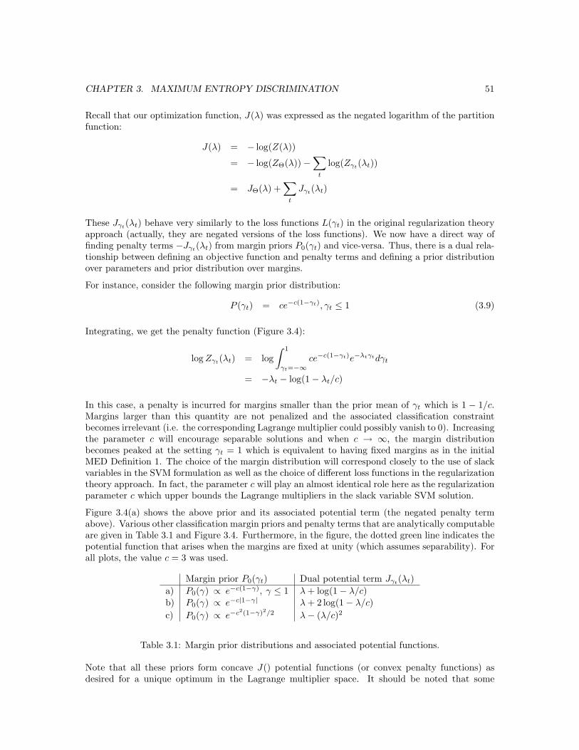
CHAPTER 3. MAXIMUM ENTROPY DISCRIMINATION 51
Recall that our optimization function, J(λ) was expressed as the negated logarithm of the partitionfunction:
J(λ) = − log(Z(λ))
= − log(ZΘ(λ))−∑
t
log(Zγt(λt))
= JΘ(λ) +∑
t
Jγt(λt)
These Jγt(λt) behave very similarly to the loss functions L(γt) in the original regularization theoryapproach (actually, they are negated versions of the loss functions). We now have a direct way offinding penalty terms −Jγt
(λt) from margin priors P0(γt) and vice-versa. Thus, there is a dual rela-tionship between defining an objective function and penalty terms and defining a prior distributionover parameters and prior distribution over margins.
For instance, consider the following margin prior distribution:
P (γt) = ce−c(1−γt), γt ≤ 1 (3.9)
Integrating, we get the penalty function (Figure 3.4):
log Zγt(λt) = log
∫ 1
γt=−∞ce−c(1−γt)e−λtγtdγt
= −λt − log(1− λt/c)
In this case, a penalty is incurred for margins smaller than the prior mean of γt which is 1 − 1/c.Margins larger than this quantity are not penalized and the associated classification constraintbecomes irrelevant (i.e. the corresponding Lagrange multiplier could possibly vanish to 0). Increasingthe parameter c will encourage separable solutions and when c → ∞, the margin distributionbecomes peaked at the setting γt = 1 which is equivalent to having fixed margins as in the initialMED Definition 1. The choice of the margin distribution will correspond closely to the use of slackvariables in the SVM formulation as well as the choice of different loss functions in the regularizationtheory approach. In fact, the parameter c will play an almost identical role here as the regularizationparameter c which upper bounds the Lagrange multipliers in the slack variable SVM solution.
Figure 3.4(a) shows the above prior and its associated potential term (the negated penalty termabove). Various other classification margin priors and penalty terms that are analytically computableare given in Table 3.1 and Figure 3.4. Furthermore, in the figure, the dotted green line indicates thepotential function that arises when the margins are fixed at unity (which assumes separability). Forall plots, the value c = 3 was used.
Margin prior P0(γt) Dual potential term Jγt(λt)
a) P0(γ) ∝ e−c(1−γ), γ ≤ 1 λ + log(1− λ/c)b) P0(γ) ∝ e−c|1−γ| λ + 2 log(1− λ/c)c) P0(γ) ∝ e−c2(1−γ)2/2 λ− (λ/c)2
Table 3.1: Margin prior distributions and associated potential functions.
Note that all these priors form concave J() potential functions (or convex penalty functions) asdesired for a unique optimum in the Lagrange multiplier space. It should be noted that some

CHAPTER 3. MAXIMUM ENTROPY DISCRIMINATION 52
−2 −1.5 −1 −0.5 0 0.5 1 1.5 20
0.5
1
1.5
2
2.5
3
3.5
4
−4 −3 −2 −1 0 1 2 30
0.1
0.2
0.3
0.4
0.5
0.6
0.7
0.8
0.9
1
−4 −3 −2 −1 0 1 2 30
0.1
0.2
0.3
0.4
0.5
0.6
0.7
0.8
0.9
1
0 0.5 1 1.5 2 2.50
0.5
1
1.5
2
2.5
0 0.5 1 1.5 2 2.5−1.5
−1
−0.5
0
0.5
1
1.5
2
2.5
0 0.5 1 1.5 2 2.50
0.5
1
1.5
2
2.5
(a) (b) (c)
Figure 3.4: Margin prior distributions (top) and associated potential functions (bottom).
potential functions will force an upper bound (via a barrier function) on the λt while others willallow them to vary freely (as long as it is non-negative). may or may not set an upper bound onthe value of λt. Other priors and penalty functions are also possible, in particular for the regressioncase which will be discussed later and which will require quite different margin configurations. Wenow move to priors for the model, in particular, priors for the bias.
3.7 Bias Priors
Bias is merely a subcomponent of the model however due to its particular interaction with thediscriminant function, it will be treated separately here. More specifically, the bias, b, appears asan additive scalar in the discriminant. Recall that Θ which can be seen as a concatenation of allparameters and thus we can consider the breakdown: Θ = {Θ/b, b}. Recall the following form ofthe discriminant functions from Equation 3.1 (or Equation 3.4):
L(X; Θ) = θT X + b
Such a bias term arises under not only in linear models but many other classification models,including generative classification, multi-class classification, and even regression models. Evidently,one can always set b to zero to remove its effect, or simply set b to a fixed constant, yet the MEDapproach easily permits us to consider a distribution over b, namely P (b) and to tailor the solutionby specifying a prior P0(b). Here, we consider two possible choices for the prior P0(b) (althoughmany others are possible): the Gaussian prior and the non-informative prior.
3.7.1 Gaussian Bias Priors
Consider the zero-mean Gaussian prior for P0(b) given by:
P0(b) =1√2πσ
e−b2
2σ2 (3.10)
This prior favors bias values that are close to zero and therefore a priori assumes an even balancebetween the two binary classes in the decision problem. If we have a prior belief that the class

CHAPTER 3. MAXIMUM ENTROPY DISCRIMINATION 53
frequencies are slightly skewed, we may introduce a mean into the above prior which would thenfavors one class over another. The resulting potential term Jb(λ) is:
Jb(λ) = − log Zb(λ)
= − log∫ b=∞
b=−∞
1√2πσ
e−b2
2σ2 e∑
tytλtbdb
= −σ2
2
(∑t
ytλt
)2
The variance (or standard deviation) σ further specifies how certain we are that the classes areevenly balanced. In terms of the potential function, it constrains with a quadratic penalty thebalance between Lagrange multipliers for the negative class and the positive class.
3.7.2 Non-Informative Bias Priors
Evidently, a Gaussian prior will favor values of b that are close to zero. However, in the absence ofany knowledge about the bias, it would be reasonable to permit any scalar value for b with equalpreference. This will give rise to a non-informative prior. This form of prior can be parameterized asa Gaussian as in Equation 3.10 but with the variance approaching infinity, i.e. σ →∞. This stretchesout the Gaussian until it starts to behave like a uniform distribution on the axis b ∈ (−∞,∞).
The resulting potential term will naturally be:
Jb(λ) = limσ→∞
−σ2
2
(∑t
ytλt
)2
Since we are to maximize the potential terms, if σ grows to infinity, the above objective functionwill go to negative infinity unless the term in the parentheses
∑t ytλt is exactly zero. Therefore, the
non-informative prior generates the extra constraint (in addition to non-negativity) on the Lagrangemultipliers requiring that
∑t ytλt = 0:
Lemma 1 If the bias prior P0(b) is set to a non-informative infinite covariance Gaussian, the(non-negative) Lagrange multipliers in the MED solution must also satisfy the following equalityconstraint:
∑t ytλt = 0
At this point, we have the defined the priors and the computational machinery necessary for theMED formulation to give rise to support vector machines.
3.8 Support Vector Machines
As previously discussed, a support vector machine can be cast in the regularization theory frameworkand is solvable as a convex program due to the fundamentally linear discriminant function it employs:
L(X; Θ) = θT X + b

CHAPTER 3. MAXIMUM ENTROPY DISCRIMINATION 54
One can also interpret the linear decision boundary generatively by considering, for example, thelog-likelihood ratio of two Gaussian distributions (one per class) with equal covariance matrices.
L(X; Θ) = logP (X|θ+)P (X|θ−)
+ b
We shall adopt the first linear discriminant boundary since it has a more efficient parameterizationand with the choice of a simple prior will exactly synthesize a support vector machine. In particular ifwe choose a Gaussian prior on the weights θ of our linear discriminant function, the MED formulationwill produce support vector machines:
Theorem 3 Assuming L(X; Θ) = θT X +b and P0(Θ, γ) = P0(θ)P0(b)P0(γ) where P0(θ) is N(0, I),P0(b) approaches a non-informative prior, and P0(γ) is given by P0(γt) as in Equation 3.9 then theLagrange multipliers λ are obtained by maximizing J(λ) subject to 0 ≤ λt ≤ c and
∑t λtyt = 0,
where
J(λ) =∑
t
[λt + log(1− λt/c) ]− 12
∑t,t′
λtλt′ytyt′(XTt Xt′)
The above J(λ) objective function is strikingly similar to the SVM dual optimization problem. Theonly difference between the two is the above formulation has an extra potential term log(1− λt/c)which acts as a barrier function preventing the λ values from growing beyond c. In an SVM, theLagrange multiplier values are clamped to be no greater than c explicitly as an extra constraintin the convex program. In both formalisms, c plays an almost identical role by varying the degreeof regularization and upper bounding the Lagrange multipliers. Typically, low c values increaseregularization, vary the sensitivity of the solution to classification errors, robustness to outliers andpermit non-separable classification problems. However, in an SVM, the c-regularization parameterarises from an ad-hoc introduction of slack variables to permit the SVM to handle non-separabledata. If we let c→ infty, the potential term log(1− λt/c) vanishes and MED gives rise to exactlyan SVM (for separable data). In practice, even for finite c, the MED and SVM solutions are almostidentical.
3.8.1 Single Axis SVM Optimization
We can greatly simplify the support vector machine by avoiding the non-informative prior on thebias. If we assume a Gaussian prior with finite covariance, the equality constraint
∑t λtyt = 0 can
be omitted. The resulting convex program only requires non-negativity on the Lagrange multipliersand the updated objective function becomes:
J(λ) =∑
t
[λt + log(1− λt/c) ] − σ2
2
(∑t
ytλt
)2
− 12
∑t,t′
λtλt′ytyt′(XTt Xt′)
Therefore, it is now possible to update a single Lagrange multiplier at a time in an axis-parallelmanner. In fact, the update for each axis is analytic (even with the MED logarithmic barrierfunction in the non-separable case). The minimal working set in this case is 1 while in the SVM,updates to increase the objective must be done simultaneously on at least 2 Lagrange multipliersas in the Sequential Minimal Optimization (SMO) technique proposed by Platt [154]. This givesthe MED implementation a simpler optimization problem which lead to gains in computationalefficiency without any significant change from the solution produced under non-informative priors.

CHAPTER 3. MAXIMUM ENTROPY DISCRIMINATION 55
3.8.2 Kernels
The MED formulation for SVMs also readily extends to the Kernel case where nonlinearities (of theKernel type) can be immediately folded in by an implicit mapping to a higher dimensional space.The updated MED objective function merely becomes:
J(λ) =∑
t
[λt + log(1− λt/c) ] − σ2
2
(∑t
ytλt
)2
− 12
∑t,t′
λtλt′ytyt′K(Xt, Xt′) (3.11)
In the above, our standard inner products of the input vectors XTt Xt′ are replaced with a kernel
function of the vectors K(Xt, Xt′) as is done in the SVM literature. The MED computationsremain relatively unchanged since (in the linear discriminant case) all calculations only involve innerproducts of the input vectors.
3.9 Generative Models
At this point we consider the use of generative models in the MED framework. This fundamen-tally extends the regularization and SVM discriminative frameworks to the powerful modeling inBayesian generative models. Herein lies the strength of the MED technique as a bridge betweentwo communities with mutually beneficial tools. Consider a two class problem where we have agenerative model for each class, namely P (X|θ+) and P (X|θ−). These two generative models canbe directly combined to form a classifier by considering their log-likelihood ratios as follows:
L(X; Θ) = logP (X|θ+)P (X|θ−)
+ b (3.12)
Here, the aggregate parameter set is Θ = {θ+, θ−, b} which includes both generative models as wellas a scalar bias. Thus, by merely changing the discriminant function, the MED framework canbe used to estimate generative models and guarantee that the decision boundary they give rise towill be optimal in a classification setting. Naturally, the above discriminant function is generallynonlinear and will give rise to a non-convex hull of constraints in a standard regularization setting.However, in the MED framework, due to the probabilistic solution P (Θ), the above discriminantfunctions still behave as a convex program.
xx x xx x
x xoo o o
o o
o ox x
oo
xx x xx x
x xoo o o
o o
o ox x
oo
(a) (b)
Figure 3.5: Discriminative Generative Models. In (a) we show the standard maximum likelihoodestimation of two generative models from the data and the resulting poor classifier decision boundarythey generate. In (b), MED moves the generators slightly such that they combine to form an accurateclassification boundary.
Estimating P (Θ) using MED will ultimately yield P (θ+, θ−, b) which can be used to specify thegenerative models for the data P (X|θ+) and P (X|θ−). These will be full generative models that

CHAPTER 3. MAXIMUM ENTROPY DISCRIMINATION 56
can be sampled from, integrated, conditioned, etc. yet unlike a direct Bayesian framework, thesegenerative models will be also combine to form a high-performance discriminative classifier whenplugged into the L(X; Θ) discriminant function. Figure 3.5(a) depicts the estimation of a maximumlikelihood generative model while MED moves the generators for each class (ellipses) such that thedecision boundary creates good classification separation in Figure 3.5(b).
Whether or not MED estimation is feasible once again hinges upon our ability to compute the log-partition function Z(λ). We will show that it is possible to obtain the partition function analyticallywhenever the generative models P (X|θ+) and P (X|θ−) are in the exponential family.
3.9.1 Exponential Family Models
We have argued that functions that can be efficiently solved within the MED approach include log-likelihood ratios of the exponential family of distributions. Can we compute the partition functionefficiently to actually implement this estimation? First we give details on the exponential familyform [9] [32]. It is well known that such distributions have important properties in maximum like-lihood estimation [9] [198]. This family subsumes a wide set of distributions and its members arecharacterized by the following general structure (commonly referred to as the natural parameteriza-tion):
p(X|θ) = exp(A(X) + XT θ −K(θ))
Where K(θ) is convex and the distribution is normalized over the space of X. Further details onthe exponential family and its many interesting properties can be found in Chapter 5 and [9] [32].In addition, each exponential family member has a conjugate prior distribution given by:
p(θ|χ) = exp(A(θ) + θT χ− K(χ))
The conjugate distribution is itself in the exponential family and therefore, its K is also convex.
Whether or not a specific combination of a discriminant function and an associated prior is estimablewithin the MED framework depends on the computability of the partition function (i.e. the objectivefunction used for optimizing the Lagrange multipliers associated with the constraints). In general,these operations will require integrals over the associated parameter distributions. In particular,recall the partition function corresponding to the binary classification case. Consider the integralover Θ in:
ZΘ(λ) =∫
P0(Θ)e∑
tλtytL(Xt|Θ)dΘ
If we now separate out the parameters associated with the class-conditional densities as well as thebias term (i.e. θ+, θ−, b) and expand the discriminant function as a log-likelihood ratio, we obtainthe following:
ZΘ =∫
P0(θ+)P0(θ−)P0(b)e∑
tλtyt[log
P (X|θ+)P (X|θ−)+b]
dΘ
The above factorizes as ZΘ = Zθ+Zθ−Zb. We can now substitute the exponential family forms forthe class-conditional distributions and associated conjugate distributions for the priors. We assumethat the prior is defined by specifying a value for χ. It suffices here to show that we can obtain

CHAPTER 3. MAXIMUM ENTROPY DISCRIMINATION 57
Zθ+ in closed form. The derivation for Zθ− is identical. We will drop the “+” symbol from Zθ+ forclarity. The problem is now reduced to evaluating:
Zθ(λ) =∫
eA(θ)+θT χ−K(χ) e∑
tλtyt(A(Xt)+XT
t θ−K(θ))dθ
We have shown earlier (see Lemma 1) that a non-informative prior over the bias term b leads to theconstraint
∑t λtyt = 0. Making this assumption, we get
Zθ(λ) = e−K(χ)+∑
tλtytA(Xt) ×
∫eA(θ)+θT (χ+
∑t
λtytXt)dθ
= e−K(χ)+∑
tλtytA(Xt) × eK(χ+
∑t
λtytXt)
The last evaluation in above results from a natural property of the exponential family. The expres-sions for A, A,K, K are known for specific distributions in the exponential family and can easilybe used to complete the above evaluation, or realize the objective function (which holds for anyexponential-family distribution):
log Zθ(λ) = K(χ +∑
t
λtytXt) +∑
t
λtytA(Xt)− K(χ)
Therefore, it is clear that we can compute the objective function J(λ) for any discriminant functionarising from exponential family generative models. In fact, integration doesn’t even need to beperformed since we have an analytic expression of our objective function in terms of the naturalparameterization for all exponential family distributions. It should also be noted that the aboveobjective function often bears a strong resemblance to the evidence term in Bayesian inference(i.e. Bayesian integration), where the Lagrange multipliers seem to act as weights on the Bayesianinference. It is straightforward at this point to perform the required optimization and find theoptimal setting of the Lagrange multipliers that maximize the concave J(λ).
3.9.2 Empirical Bayes Priors
At this point, we have proven that it is feasible to estimate generative models in the exponentialfamily form under MED if we assume the priors are given by the conjugate distribution. However,the parameters of the conjugate priors are still not specified and we still have quite some flexibilityin designing prior knowledge into the MED formulation. In the absence of any prior knowledge, andwhenever possible we recommend the default prior to be either a conjugate non-informative prior oran Empirical Bayes prior.
Loosely put, the prior for P0(Θ), or more specifically for P0(θ+) and P0(θ−), we will use will be theposterior distribution of the parameters given the data that Bayesian inference generates. Considerthe data set {X1, . . . , XT } with binary (±1) labels {y1, . . . , yT }. Thus, the inputs can be split intothe positive inputs {X1+, . . . , XT+} and the negative inputs {X1−, . . . , XT−}.
We now explicate the Bayesian inference procedure. To distinguish the resulting densities from thosethat will be used in the MED formulation, here we will put a P symbol on the Bayesian distributions.In Bayesian inference, each class’s posterior distribution is estimated only from the positive inputexemplars {X1+, . . . , XT+} as follows:
P (θ+) = P (θ+|{X1+, . . . , XT+})= P ({X1+, . . . , XT+}|θ+)P (θ+)= Πt+P (Xt+|θ+)P0(θ+)

CHAPTER 3. MAXIMUM ENTROPY DISCRIMINATION 58
Similarly, the negative class’s generative Bayesian posterior model is estimated only from the negativeinput exemplars {X1−, . . . , XT−} :
P (θ−) = Πt−P (Xt−|θ−)P0(θ−)
For this Bayesian estimate of the generative model of the data, a minimally informative prior P0(θ±)should be used. The result is a distribution that is as good a generator as possible for the data set.
However, we don’t want just a good generator of the data, we also want a good discriminator.Thus, we can use MED to satisfy the large-margin classification constraints. But, simultaneously,the solution should be as close as possible to the generative model in terms of KL-divergence.Therefore, we shall use the Bayesian posteriors as the MED priors!
P0(θ+) := P (θ+)P0(θ−) := P (θ−)
Figure 3.6 depicts the information projection solution MED will generate from the Bayesian estimate.Effectively, we will try solving for the distribution over parameters that is as close as possible to theBayesian estimate (which is often actually quite similar to the maximum likelihood estimate in thecase of the exponential family) but that also satisfies the classification constraints.
*
MED P(Θ)
BAYES P(Θ)
*P
Figure 3.6: Information Projection Operation of the Bayesian Generative Estimate.
The motivation here is that in the absence of any further discriminative information, we should haveas good a generator as possible. We now note a number of advantages for this type of empirical Bayesprior, that include theoretical, conceptual and practical arguments.. First, an empirical Bayes prioris a good precautionary measure to take because it allows more flexible use of MED’s discriminativemodel as a generator whenever necessary. This may be the case when the discriminator has tocope with missing data or noise. If, therefore, we are in a prediction setting where some inputvariables are missing, we could reconstruct them (or integrate over them) by simply using the MEDdiscriminative model as a surrogate for a generator distribution.
Under sparse data situations a model may easily satisfy some given discrimination constraints andmany aspects of the model could remain ambiguous. In these cases, the empirical Bayesian priorprovides a backup generative criterion, which further constrains the problem (albeit in ways nothelpful to the task) and therefore can help consistent estimation. We also obtain an invariance inusing an empirical Bayes prior that we would not get if we assume a fixed prior. For example, a

CHAPTER 3. MAXIMUM ENTROPY DISCRIMINATION 59
fixed zero-mean Gaussian prior would produce different MED solutions if we translate the trainingdata while an empirical Bayes prior would follow the translation of the data (with the Bayesiangenerative model) and consistently setup the same relative decision boundary.
Furthermore, consistency is important under the (arguably over-optimistic) situation that the gen-erative model we are using is exactly correct and perfectly matches the training data. In that case,the Bayesian solution is optimal and MED may stray from it unless we have an empirical Bayesprior, even if we obtain infinite training data. An interesting side note is that if we use the standardmargin prior distribution given by Equation 3.9, and obtain an upper bound on the Lagrange mul-tipliers (i.e. they are < c), then as c→ 0, the MED solution uses the Bayesian posterior while as cincreases, we reduce regularization (and outlier rejection) in favor of perfect classification.
Finally, on a purely practical note, an empirical Bayes prior may provide better numerical stability,for example. A discriminative MED model could put little probability mass on the training dataand return a very poor generative configuration while still perfectly separating the data. This wouldbe undesirable numerically since we would get very small values for, eg. P (X|θ+) and P (X|θ−).During prediction, a new test point may cause numerical accuracy problems if it is far from theprobability mass in the MED discriminative solution. Therefore, whenever it does not result in aloss of discriminative power, one should maintain the generative aspects of the model.
3.9.3 Full Covariance Gaussians
We now consider the case where the discriminant function L(X; Θ) corresponds to the log-likelihoodratio of two Gaussians with different (and adjustable) covariance matrices. The parameters Θ in thiscase are both the means and the covariances. These generative models are within the exponentialfamily and so the previous results hold. Thus, the prior of choice P0(Θ) must be the conjugateto the full-covariance Gaussian which is the Normal-Wishart. We shall use N as shorthand forthe normal distribution and IW as shorthand for the inverse-Wishart. This choice of distributionspermits us to obtain closed form integrals for the partition function Z(λ). Here, we shall once againbreakdown the parameters into the two generative models and the bias as before. Thus, we haveP (Θ) = P (θ+)P (θ−)P (b). More specifically, the θ± will also be broken down into the mean andcovariance components of the Gaussian. Therefore, we have: P (Θ) = P (µ+,Σ+)P (µ−,Σ−)P (b)which gives us a density over means and covariances (this notation closely follows that of [136]).
The prior distribution has the form
P0(θ+) = N (µ+|m+,Σ+/k) IW(Σ+|kV+, k)
Where the parameters that specify the prior, namely the scalar k, the vector m+, and the matrixV+ can be imputed manually. Also, one may let k → 0 to get a non-informative prior.
We used the MAP values for k, m0 and V0 from the class-specific data which corresponds to theposterior distribution over the parameters given the data under a Bayesian inference procedure (i.e.an empirical Bayes procedure as described in the previous section). Integrating over the parameters,we get the partition function which factorizes Z(λ) = Zγ(λ)Z+(λ)Z−(λ). For Z+(λ) we obtain thefollowing:
Z+(λ) ∝ N−d/2+ |πS+|−N+/2 Πd
j=1Γ(
N+ + 1− j
2
)
In the above we have defined the following intermediate variables (the scalar N+, the vector X+ and

CHAPTER 3. MAXIMUM ENTROPY DISCRIMINATION 60
the matrix S+) for brevity:
N+∆=
∑t
wt
X+∆=
∑t
wt
N+Xt
S+4=
∑t
wtXtXTt −N+X+XT
+
Here, wt is a scalar weight given by wt = u(yt) + ytλt for Z+(λ). To solve for Z−(λ) we proceed inexactly the same manner as above however here, the weights are set to wt = u(−yt)−ytλt. The u(·)is merely the step function. Given Z, updating λ is done by maximizing the corresponding negativeentropy J(λ) subject to 0 ≤ λt ≤ c and
∑t λtyt = 0 where:
J(λ) =∑
t
[lαλt + log(1− λt/c)]− log Z+(λt)− log Z−(λt)
The potential term above corresponds to integrating over the margin with a margin prior P0(γ) ∝e−c(lα−γ) with γ ≤ s. We pick lα to be some α-percentile of the margins obtained under the standardMAP solution.
Optimal Lagrange multiplier values are then found via a simple constrained gradient descent proce-dure. The resulting MRE (normalized by the partition function Z(λ)) is a Normal-Wishart distri-bution itself for each generative model with the final λ values set by the maximization of J(λ):
P (θ+) = N (µ+; X+,Σ+/N+) IW(Σ+;S+, N+)
Predicting the labels for a data point X under the final P (Θ) involves taking expectations of thediscriminant function under a Normal-Wishart. For the positive generative class, this expectationis:
EP (θ+) [log P (X|θ+)] = constant− N+
2(X − X+)T S−1
+ (X − X+)
The expectation over the negative class is similar. This gives us the predicted label quite simply as:
y = sign∫
P (Θ)L(X; Θ)dΘ
y = sign EP (Θ)
[log
P (X|θ+)P (X|θ−)
+ b
]y = sign
(EP (θ+) [log P (X|θ+)]− EP (θ−) [log P (X|θ−)] + EP (b) [b]
)Computing the expectation over the bias is avoided under the non-informative case and the additiveeffect it has is merely estimated as in an SVM via the Karush-Kuhn-Tucker conditions. We thusobtain discriminative quadratic decision boundaries. These extend the linear boundaries without(explicitly) resorting to kernels. Of course, kernels may still be used in this formalism, effectivelymapping the feature space into a higher dimensional representation. However, unlike linear dis-crimination, the covariance estimation in this framework allows the model to adaptively modify thekernel.
For visualization, we present the technique on a 2D set of training data in Figure 3.7. In Figure 3.7(a),the maximum likelihood technique is used to estimate a 2 Gaussian discrimination boundary (bias is

CHAPTER 3. MAXIMUM ENTROPY DISCRIMINATION 61
(a) ML & MED Initialization (b) MED Intermediate
(c) MED Intermediate (d) MED Converged
Figure 3.7: Classification visualization for Gaussian discrimination.
estimated separately) which has the flexibility to achieve perfect classification yet produces a classifierwhose performance is equal to random guessing. Meanwhile, the maximum entropy discriminationtechnique places the Gaussians in the most discriminative configuration as shown in Figure 3.7(b)without requiring kernels or feature space manipulations.
Experiments
In the following, we show results using the minimum relative entropy approach where the discrim-inant function L(X, Θ) is the log-ratio of Gaussians with variable covariance matrices on standard2-class classification problems (Leptograpsus Crabs and Breast Cancer Wisconsin). Performance iscompared to regular support vector machines, maximum likelihood estimation and other methods.
The Leptograpsus crabs data set was originally provided by Ripley [162] and further tested byBarber and Williams [8]. The objective is to classify the sex of the crabs from 5 scalar anatomicalobservations. The training set contains 80 examples (40 of each sex) and the test set includes 120examples.
The Gaussian based decision boundaries are compared in Table 3.2 against other models from[8].The table shows that the maximum entropy (or minimum relative entropy) criterion improves theGaussian discrimination performance to levels similar to the best alternative models. The bias wasestimated separately from training data for both the maximum likelihood Gaussian models and themaximum entropy discrimination case. In addition, we show the performance of a support vectormachine (SVM) with linear, radial basis and polynomial decision boundaries (using the Matlab SVMToolbox provided by Steve Gunn). In this case, the linear SVM is limited in flexibility while kernelsexhibit some over-fitting.

CHAPTER 3. MAXIMUM ENTROPY DISCRIMINATION 62
Method Training TestingErrors Errors
Neural Network (1) 3Neural Network (2) 3Linear Discriminant 8Logistic Regression 4MARS (degree = 1) 4PP (4 ridge functions) 6Gaussian Process (HMC) 3Gaussian Process (MAP) 3SVM - Linear 5 3SVM - RBF σ = 0.3 1 18SVM - 3rd Order Polynomial 3 6Maximum Likelihood Gaussians 4 7MaxEnt Discrimination Gaussians 2 3
Table 3.2: Leptograpsus Crabs
Another data set which was tested was the Breast Cancer Wisconsin data where the two classes(malignant or benign) have to be computed from 9 numerical attributes from the patients’ tumors(200 training cases and 169 test cases). The data was first presented by Wolberg [206]. We compareour results to those produced by Zhang [211] who used a nearest neighbor algorithm to achieve 93.7%accuracy. As can be seen from Table 3.3, over-fitting prevents good performance from the kernelbased SVMs and the top performer here is the maximum entropy discriminator with an accuracy of95.3%.
Method Training TestingErrors Errors
Nearest Neighbor 11SVM - Linear 8 10SVM - RBF σ = 0.3 0 11SVM - 3rd Order Polynomial 1 13Maximum Likelihood Gaussians 10 16MaxEnt Discrimination Gaussians 3 8
Table 3.3: Breast Cancer Classification
3.9.4 Multinomials
Another popular exponential family model is the multinomial distribution. We next consider the casewhere the discriminant function L(X; Θ) corresponds to the log-likelihood ratio of two multinomials:
L(X; Θ) = logP (X|θ+)P (X|θ−)
− b
Where we have the generative models given by (if the X vector is consider as a set of counts):
P (X|θ+) =( ∑K
k=1 Xk
X1 . . . XK
)ΠK
k=1ρXk
k (3.13)
In the above, we are using the superscript on Xk to index into the dimensionality of the vector (thesubscript will be used to index into the training set). The scalar term in the large parentheses is
CHAPTER 3. MAXIMUM ENTROPY DISCRIMINATION 63
the multinomial coefficient (the natural extension of the binomial coefficient from coin tossing todie tossing). This scalar term is unity if the X vector is zero everywhere except for one unit entry.Otherwise it simply scales the probability distribution by a constant factor which can be rewrittenas follows for more clarity (the use of gamma functions permits us to also consider continuous Xvectors):
( ∑Kk=1 Xk
X1 . . . XK
)=
(∑Kk=1 Xk
)!
ΠKk=1X
k!=
Γ(1 +∑K
k=1 Xk)ΠK
k=1Γ(1 + Xk)
The generative distribution in Equation 3.13 parameterizes the multinomial with the ρ vector ofnon-negative scalars that sum to unity, i.e.
∑ρ = 1. The parameters Θ in this case are both the ρ
for the positive class and the negative class as well as the bias scalar b. These generative models arewithin the exponential family and so the previous results hold. Thus, the prior of choice P0(Θ) mustbe the conjugate to the multinomial which is the Dirichlet distribution. This choice of distributionspermits us to obtain closed form integrals for the partition function Z(λ). Here, we shall once againbreakdown the parameters into the two generative models and the bias as before. Thus, we haveP (Θ) = P (θ+)P (θ−)P (b), to distinguish the ρ for the positive class, we will denote the parametersfor the negative class as ρ. The prior Dirichlet distribution has the form
P0(θ+) =Γ(∑
k αk)ΠkΓ(αk)
Πkραk−1k
We typically assume that αk will be pre-specified manually (or given by an empirical Bayes pro-cedure) and will satisfy αk > 1. The core computation involves computing the component of thelog-partition function that corresponds to the model (the computation for the bias and the marginsremain the same as all the previous cases). Thus, we need:
Zθ+(λ)Zθ−(λ) =∫
P0(θ+)P0(θ−)e∑
tλtyt[log
P (Xt|θ+)P (Xt|θ−) ]dθ+dθ−
It suffices to show how to compute Zθ+ :
Zθ+ =∫
P0(θ+)e∑
tλtyt log P (Xt|θ+)dθ+
=∫
Γ(∑
k αk)ΠkΓ(αk)
Πkραk−1k e
∑t
λtyt log
( ∑k Xk
t
Xkt . . . Xk
t
)+∑
tλtyt log Πkρ
Xkt
k
dρ
=∫
Γ(∑
k αk)ΠkΓ(αk)
Πkραk−1k e
∑t
λtyt log ΠkρXk
tk dρ × e
∑t
λtyt log
( ∑k Xk
t
X1t . . . XK
t
)
=∫
Γ(∑
k αk)ΠkΓ(αk)
Πkραk−1k Πkρ
∑t
λtytXkt
k dρ × e
∑t
λtyt log
( ∑k Xk
t
X1t . . . XK
t
)
=∫
Γ(∑
k αk)ΠkΓ(αk)
Πkραk−1+
∑t
λtytXkt
k dρ × e
∑t
λtyt log
( ∑k Xk
t
X1t . . . XK
t
)
=Γ(∑
k αk)Γ(∑
k αk +∑
tk λtytXkt )
ΠkΓ(αk +
∑t λtytX
kt )
Γ(αk)× e
∑t
λtyt log
( ∑k Xk
t
X1t . . . XK
t
)
CHAPTER 3. MAXIMUM ENTROPY DISCRIMINATION 64
We can thus form our objective function and maximize it to obtain the setting for the Lagrangemultipliers λ (subject to the constraint
∑t λtyt = 0):
J(λ) = − log Zθ+(λ)− log Zθ−(λ)− log Zγ(λ)
The setting for the Lagrange multipliers permits us to exactly specify the final MED solution dis-tribution P (Θ) which is used to compute the predictions for future classification:
y = sign∫
P (Θ)L(X; Θ)dΘ
3.10 Generalization Guarantees
We now present several arguments for MED in terms of generalization guarantees. While generativeframeworks have guarantees (asymptotic and otherwise) on the goodness of fit of a distribution(i.e. Bayesian evidence score, Bayesian Information Criterion, Akaike Information Criterion, etc.),they seldom have guarantees on the generalization performance of the models in a classificationor regression setting. Furthermore, the guarantees may be distribution dependent which might beinappropriate if the true generative distribution of a data source is not perfectly known. Conversely,discriminative approaches that specifically target the classification or regression performance canhave strong generalization arguments as we move from training data to testing data. These may alsobe distribution independent. The MED framework, in its discriminative estimation approach, bringsclassification performance guarantees to generative models. There are a number of arguments we willmake, including sparsity-based generalization, references to VC-dimension based generalization andPAC-Bayesian generalization. Although generalization bounds can be quite loose for small amountsof training data, they are better than no guarantees whatsoever. Furthermore, the ’shape’ of thegeneralization bounds have been demonstrated empirically to be useful in a discriminative setting.Finally, under large amounts of data, these bounds could be reasonably tight.
3.10.1 VC Dimension
Due to the ability of the MED framework to subsume SVMs (exactly generating the same equationsin the separable case), it too benefits from the generalization guarantees that accompany them.These are of course the VC-dimension (Vapnik-Chervonenkis) bounds on the expected risk, R(Θ),of a classifier. Assuming we have a [0, 1] loss function l(Xt, yt,Θ) and T training exemplars, theempirical risk can be readily computed [35] [196] [197]:
Remp(Θ) =1T
T∑t=1
l(Xt, yt,Θ)
The true risk (for samples outside of the training set) is then bounded above by the empirical plusa term that depends only on the size of training set, T and the VC-dimension of the classifier, h.This non-negative integer quantity measures the capacity of a classifier and is independent of thedistribution of the data. The following bound holds with probability 1− δ:
R(Θ) ≤ Remp(Θ) +
√h(log(2T/h) + 1)− log(δ/4)
T
The VC-dimension of a set of hyper-planes in <n is equal n+1. This does not directly motivate theuse of large margin decision boundaries in an SVM. However, an SVM can be interpreted instead as

CHAPTER 3. MAXIMUM ENTROPY DISCRIMINATION 65
a gap-tolerant classifier instead of a pure hyper-plane. A gap-tolerant classifier is a set of two parallelhyper-planes with a sphere. All points outside the sphere and all points between the planes do notcontribute to the risk while points within the sphere and on either side of the planes are assigneda class (i.e. ±1). Thus, if all points are within the sphere and outside of the two hyper-planes,the VC-dimension can be upper bounded by the radius of the resulting sphere R and the marginbetween the planes M . This gives the following upper bound on the VC-dimension, h, in an featurespace of <n:
h ≤ max{
D2
M2, n
}+ 1
Thus, we have a ’plausible’ argument for maximizing margin with a linear classifier. Although thisdoes not translate immediately to nonlinear classifiers (if there is no direct kernel mapping back tolinear hyper-planes), the motivation for large-margin in SVMs still can be used to justify using largemargins in the MED formulation (namely with priors put large probability mass on larger marginsvalues). We now move to other formal arguments for MED generalization.
3.10.2 Sparsity
The MED solution involves a constraint-based optimization where a classification constraint ispresent over each training data point to be classified. Each constraint is represented by the La-grange multiplier associated with the given data point. In many cases, these constraints are likelyto be redundant. This is apparent since classifying one data point correctly might automaticallyresult in correct classification of several others. Therefore, the constraints involving some data pointswill be obviated by others and their corresponding Lagrange multipliers will go to zero. As in anSVM, points close to the margin (which have small margin values) have a critical role in shapingthe decision boundary and generate non-zero Lagrange multipliers. These are the support-vectors inthe standard SVM terminology. Meanwhile, other points that are easily correctly classified with alarge margin will have zero Lagrange multipliers. Thus, the MED solution only depends on a smallsubset of the training data and will not change if the other data points were deleted. This gives riseto a notion of sparsity and with it we can make some generalization arguments. One argument isthat the generalization error (denoted εg) is less than the expected percentage (ratio) of non-zeroLagrange multipliers over all Lagrange multipliers.
εg ≤ E
[∑Tt=1 δ(λt > 0)
T
]
Thus, for T data points, we simply count the number of non-zero Lagrange multipliers (using theδ function which is zero for Lagrange multipliers of value zero and unity for non-vanishing values).However, the expectation is taken over arbitrary choices of the training set which means that theupper bound on generalization error can only be approximated (using cross-validation or othertechniques as in [196] [83]). Alternatively, a coarse and riskier approximation to the expectation canbe done by simply counting the number of remaining non-zero Lagrange multipliers after maximizingJ(λ) on the training set in the MED solution.
3.10.3 PAC-Bayes Bounds
An alternative to VC dimension arguments for generalization includes PAC bounds (probably ap-proximately correct, Valiant 1984). Recent contributions in terms of a PAC-Bayesian model selection

CHAPTER 3. MAXIMUM ENTROPY DISCRIMINATION 66
criteria by McAllester [125] and Langford [116] have given theoretical generalization arguments thatdirectly motivate the MED approach (MED was actually developed prior to the generalization re-sults). Essentially PAC-Bayesian approaches allow the combination of a Bayesian integration ofprior domain knowledge with PAC generalization guarantees without forcing the PAC frameworkto assume the truthfulness of the prior. We loosely adapt and state the main results of [116] herebut further details are available from the original work as well as [125]. Effectively, the gener-alization guarantees are for model averaging where a stochastic model selection criterion is givenin favor of a deterministic one. MED is a model averaging framework in that a distribution overmodels is computed (unlike, eg. an SVM). Therefore, these new generalization results apply almostimmediately.
First, (as in MED) we assume a prior probability distribution P0(Θ) over a possibly uncount-able (continuous) model class. We also assume our discriminant functions L(X; Θ) are boundedreal-valued hypotheses 7. Given a set T training exemplars of the form (Xt, yt) sampled from adistribution D, we would like to compute the expected loss (i.e. the fraction of misclassifications)over the true distribution D. Recall in MED that a correct classification of the data is given by:
yt
∫P (Θ)L(Xt; Θ)dΘ ≥ 0
Meanwhile, incorrect classifications are of the form:
yt
∫P (Θ)L(Xt; Θ)dΘ ≤ 0
A more conservative empirical misclassification rate (i.e. which over counts the number of errors)can be made by also counting those errors below some positive margin threshold γ:
yt
∫P (Θ)L(Xt; Θ)dΘ ≤ γ
If we compute the empirical number of misclassifications with this more conservative technique basedon the margin threshold, γ, we can upper bound the expected (standard) misclassification rate. Theexpected misclassification rate has the following upper bound bound which holds with probability1− δ:
ED
[y
∫P (Θ)L(X; Θ)dΘ ≤ 0
]≤ 1
T
∑t
[yt
∫P (Θ)L(Xt; Θ)dΘ ≤ γ
]
+O
(√γ−2D(P (Θ)‖P0(Θ)) lnT + lnT + ln δ−1
T
)
Ideally, we would like to minimize the expected risk of the classifier on future data (left hand side).Clearly, the bound above motivates forming a classifier that satisfies the empirical classificationconstraints (encapsulated by the first term on the right hand side), while minimizing divergence to theprior distribution (the second term on the right hand side). We also note that increasing the margin
7The generalization guarantees were actually originally for averaging binary discriminant functions, not real ones,but can be extended to real ones in a straightforward manner. One may construct an MED classifier where thediscriminant function is, eg. sigmoidal, or binary and then satisfy the requirements for these bounds to hold. Alter-natively, a trivial extension is to find a bound by considering a maximal sphere around all the data which implicitlyprovides limits on the range of the discriminant function. This then permits a scaled version of the generalizationbound.

CHAPTER 3. MAXIMUM ENTROPY DISCRIMINATION 67
threshold is also useful at minimizing the expected risk. These criteria are directly addressed by theMED framework which strongly agrees with this theoretical motivation. Furthermore, increasing thecardinality of the training data set will make the bound tighter independently of the distribution ofthe data. Another point of contact is that [125] argues that the optimal posterior according to thesetypes of bounds is, as in the Maximum Entropy Discrimination solution, the Gibbs distribution.
3.11 Summary and Extensions
We have presented the Maximum Entropy Discrimination framework from a regularization theoryperspective and shown how it subsumes support vector machines. The solvability of the MEDsolution has been demonstrated. We have also shown how MED can readily be used in a generativeframework where decision boundaries arise from exponential family distributions over the inputspace. Finally, generalization guarantees provide the framework with a theoretical grounding thatreinforces its flexibility and generality. We next discuss the many extensions that can now becascaded into the MED formalism which further motivate the usefulness of the approach.

Chapter 4
Extensions to Maximum EntropyDiscrimination
Up to this point the MED formulation has already bridged generative modeling with the discrim-inative performance of SVMs, for example. However, the MED method can be further elaboratedand spans a wide range of machine learning scenarios. In this chapter, we discuss various exten-sions to the framework to demonstrate its flexibility and intuitive nature. One resounding themin exploring extensions is to introduce further (possibly intermediate) variables in the discriminantfunction L(X; Θ) and to solve for an augmented distribution P (Θ, . . .) that includes them. Theresulting partition function typically involves more integration yet if it is analytic and the number ofLagrange multipliers and the optimization complexity will remain basically unchanged. Figure 4.1depicts the common metaphor of augmenting the probability with further variables which will beutilized. This follows the same principle used to augment the distribution with soft margin con-straints as in Section 3.3. Once again, we note the caveat that as we add more distributions to theprior, we should be careful to balance their competing goals (i.e. their variances) evenly so thatwe still derive meaningful information from each component of the aggregate prior (i.e. the modelprior, the margin prior, and the many further priors we will introduce shortly).
*
P(Θ,γ,s,y,X,...)
P0(Θ,γ,s,y,X,...)
*P
Figure 4.1: Formulating extensions to MED.
Figure 4.2 depicts the many different scenarios the MED can handle. Some extensions such asmulti-class classification can be treated as several binary classification constraints [85] or througherror-correcting codes [45]. In this chapter we explicate the case where the labels are no longerdiscrete but continuous, i.e. regression. Once again, for the case of regression (just as in binary
68

CHAPTER 4. EXTENSIONS TO MAXIMUM ENTROPY DISCRIMINATION 69
classification) the SVM regression is subsumed. Subsequently, we discuss structure learning (asopposed to parameter estimation) in particular for feature selection applications. Furthermore, wediscuss the use of partially labeled examples and transduction (for both classification and regression).Finally, we lead into a very important generalization which requires special treatment on its own:extension to mixture models (i.e. mixtures of the exponential family) and latent modeling (discussedChapter 5).
x ox
xx
oo
oo+
x o
xxx
oooo
+++
+
xx x
xx
xx
x
(a) Binary Classification (b) Multiclass Classification (c) Regression
x ox
xx
oooox ox xx oooo
x ox
xxo
oo
o???
?
??
??
?
x
x x
xxxxx xx
x
x
(d) Feature Selection (e) Transduction (f) Anomaly Detection
Figure 4.2: Various extensions to binary classification.
4.1 MED Regression
The MED formalism is not restricted to classification. Here, we present its extension to the regres-sion (or function approximation) case using the approach and nomenclature in [178]. Dual sidedconstraints are imposed on the output such that an interval called an ε-tube around the functionis described 1. Suppose training input examples {X1, . . . , XT } are given with their correspondingoutput values as continuous scalars {y1, . . . , yT }. We wish to solve for a distribution of parametersof a discriminative regression function as well as margin variables:
Theorem 4 The maximum entropy discrimination regression problem can be cast as follows:
Find P (Θ, γ) that minimizes KL(P‖P0) subject to the constraints:∫P (Θ, γ) [yt − L(Xt; Θ) + γt] dΘdγ ≥ 0, t = 1..T∫P (Θ, γ) [γ′t − yt + L(Xt; Θ)] dΘdγ ≥ 0, t = 1..T
1An ε-tube (as in the SVM literature) is a region of insensitivity in the loss function which only penalizes approx-imation errors which deviate by more than ε from the data.

CHAPTER 4. EXTENSIONS TO MAXIMUM ENTROPY DISCRIMINATION 70
−1 −0.5 0 0.5 1 1.5 2 2.5 3 3.5 40
0.5
1
1.5
2
2.5
3
3.5
4
−1 −0.5 0 0.5 1 1.5 2 2.5 3 3.5 40
0.5
1
1.5
2
2.5
3
3.5
4
−1 −0.5 0 0.5 1 1.5 2 2.5 3 3.5 40
0.5
1
1.5
2
2.5
3
3.5
4
0 0.5 1 1.5 2 2.5 3−5
−4
−3
−2
−1
0
1
2
0 10 20 30 40 500
10
20
30
40
50
60
0 0.5 1 1.5 2 2.5 31
1.5
2
2.5
3
3.5
4
4.5
(a) (b) (c)
Figure 4.3: Margin prior distributions (top) and associated potential functions (bottom).
where L(Xt; Θ) is a discriminant function and P0 is a prior distribution over models and margins.The decision rule is given by y =
∫P (Θ) L(X; Θ)dΘ. The solution is given by:
P (Θ, γ) =1
Z(λ)P0(Θ, γ)
e∑
tλt[ yt−L(Xt|Θ)+γt]
e∑
tλ′t[ yt−L(Xt|Θ)−γ′t]
where the objective function is again J(λ) = − log Z(λ).
Typically, we have the following prior for γ which differs from the classification case due to theadditive role of the output yt (versus multiplicative) and the two-sided constraints.
P0(γt) ∝{
1 if 0 ≤ γt ≤ εec(ε−γt) if γt > ε
}(4.1)
Integrating, we obtain:
log Zγt(λt) = log(∫ ε
0
eλtγtdγt +∫ ∞
ε
ec(ε−γt)eλtγtdγt
)= log
(eλε
λ− 1
λ+
eλε
c− λ
)= log
((eλε
λ
)(1− e−λε +
λ
c− λ
))= ελt − log(λt) + log
(1− e−λtε +
λt
c− λt
)
Figure 4.3 shows the above prior and its associated penalty terms under different settings of c and ε.Varying ε effectively modifies the thickness of the ε-tube around the function. Furthermore, c variesthe robustness to outliers by tolerating violations of the ε-tube.
The above margin prior tends to produce a regressor which is insensitive to errors smaller than εand then penalizes errors by an almost linear loss thereafter (where c controls the steepness of thelinear loss).

CHAPTER 4. EXTENSIONS TO MAXIMUM ENTROPY DISCRIMINATION 71
−10 −5 0 5 10−0.4
−0.2
0
0.2
0.4
0.6
0.8
1
1.2
−10 −5 0 5 10−0.4
−0.2
0
0.2
0.4
0.6
0.8
1
1.2
Figure 4.4: MED approximation to the sinc function: noise-free case (left) and with Gaussian noise(right).
4.1.1 SVM Regression
If we assume a linear discriminant function for L (or linear decision after a Kernel), the MEDformulation generates the same objective function that arises in SVM regression [178]:
Theorem 5 Assuming L(X; Θ) = θT X +b and P0(Θ, γ) = P0(θ)P0(b)P0(γ) where P0(θ) is N(0, I),P0(b) approaches a non-informative prior, and P0(γ) is given by Equation 4.1 then the Lagrangemultipliers λ are obtained by maximizing J(λ) subject to 0 ≤ λt ≤ c, 0 ≤ λ′t ≤ c and
∑t λt =
∑t λ′t,
where
J(λ) =∑
t
yt(λ′t − λt)− ε∑
t
(λt + λ′t) +∑
t
log(λt)− log(
1− e−λtε +λt
c− λt
)+∑
t
log(λ′t)− log(
1− e−λ′tε +λ′t
c− λ′t
)− 1
2
∑t,t′
(λt − λ′t)(λt′ − λ′t′)(XTt Xt′)
As can be seen (and more so as c → ∞), the objective becomes very similar to the one in SVMregression. There are some additional penalty functions (all the logarithmic terms) which can beconsidered as barrier functions in the optimization to maintain the constraints.
To illustrate the regression, we approximate the sinc function, a popular example in the SVMliterature. Here, we sampled 100 points from the sinc(x) = |x|−1 sin |x| within the interval [-10,10].We also considered a noisy version of the sinc function where Gaussian additive noise of standarddeviation 0.2 was added to the output. Figure 4.4 shows the resulting function approximation whichis very similar to the SVM case. The Kernel applied was an 8th order polynomial 2.
4.1.2 Generative Model Regression
As was the case for MED classification, we can also consider an MED regression scenario where theregression model is not linear (or linear after some kernel manipulation) but actually the regressionmodel is given by a probability distribution. Thus, the regularization and epsilon-tube propertiesof the SVM approach can be readily applied to the estimation of generative models in a regressionsetting. Furthermore, these can be in the exponential family and also mixtures of the exponential
2A Kernel implicitly transforms the input data by modifying the dot-product between data vectors k(Xt, X′t) =
〈Φ(Xt), Φ(X′t)〉. This can also be done by explicitly remapping the data via the transformation Φ(Xt) and using the
conventional dot-product. This permits non-linear classification and regression using the basic linear SVM machinery.For example, an m-th order polynomial expansion replaces a vector Xt by Φ(Xt) = [Xt; X2
t ; . . . Xmt ].

CHAPTER 4. EXTENSIONS TO MAXIMUM ENTROPY DISCRIMINATION 72
family as will be elaborated in the subsequent chapter. We begin by modifying the discriminantfunction L(X; Θ) from its usual linear form.
Consider a two class problem where we have a generative model for each class, namely P (X|θ+) andP (X|θ−). For example, these could each be a Gaussian distribution, or a mixture of Gaussians oreven a complex structured model such as a hidden Markov model. To form a regressor, we directlycombine two generative models by considering their log-likelihood ratios into a discriminant functionas follows:
L(X; Θ) = logP (X|θ+)P (X|θ−)
+ b
Here, the aggregate parameter set is Θ = {θ+, θ−, b} which includes both generative models as wellas a scalar bias. Thus, by merely changing the discriminant function, the MED framework canbe used to estimate generative models that form a regression function. If the two generators areGaussians with equal covariance, the regression function will effectively produce a linear regression.However, the above discriminant function is generally nonlinear and will give rise to a non-convexhull of constraints in a standard regularization setting. However, in the MED framework, due tothe probabilistic solution P (Θ), the above discriminant functions still behave as a convex program.Furthermore, it is possible (through the iterative bounds and machinery in Chapter 5) to deal withlatent discriminant regression functions of the form:
L(X; Θ) = log∑
m P (m,X|θ+)∑m P (m,X|θ−)
+ b
4.2 Feature Selection and Structure Learning
The MED framework is not limited to estimating distributions over continuous parameters such asΘ. We can also use it to solve for a distribution over discrete parameters and thus use it for structurelearning. One form of structure learning is feature selection. The feature selection problem can becast as finding the structure of a graphical model (as in [43]) or identifying a set of components ofthe input examples that are relevant for a classification task. More generally, feature selection can beviewed as a problem of setting discrete structural parameters associated with a specific classificationor regression method. We will use feature selection in the MED framework to ignore components ofthe input space (i.e. the Xt vectors) that are not relevant to the given classification or regressiontask. This will naturally provide computational advantages since the algorithm can ignore theseinputs during run-time. However, not only does feature selection reduce the input dimensionality,we will also show that it helps improve generalization accuracy in both classification and regression(cf. [111]). The omission of certain input dimensions permits better generalization and leads to afurther notion of sparsity in the input dimensionality (in addition to the sparsity from the supportvectors and Lagrange multipliers as discussed in Section 3.10.2) [90] [202]. This is often critical ifthe input space has high dimensionality, many irrelevant features and the data set is small.
We will initially derive the feature selection in the MED framework as a feature weighting to permit aprobabilistic solution. Each feature or structural parameter is given a probability value. The featureselection process then estimates the most discriminative probability distribution over the structuralparameters while it also estimates the most discriminative parameter model. Irrelevant features willeventually receive extremely low probabilities of being selected. Since the feature selection process isperformed jointly and discriminatively together with model estimation and both specifically optimizea classification or regression criterion, feature selection will usually improve results over, for example,an SVM (up to a point where we start removing too many features).
CHAPTER 4. EXTENSIONS TO MAXIMUM ENTROPY DISCRIMINATION 73
4.2.1 Feature Selection in Classification
The MED formulation can be extended to feature selection if we consider augmenting the distribu-tion over models (and margins, bias, etc.) also with a distribution over feature selection switches.This ’augmentation’ paradigm was initially discussed in Section 3.3 and under many conditions willpreserve the solvability of the MED projection. We will now consider augmenting a linear classi-fier (such as an SVM) with feature selection. We first introduce extra parameters into our lineardiscriminant function:
L(X; Θ) =n∑
i=1
θisiXi + θ0
Here, the familiar θ1, . . . , θn correspond to the linear parameter vector while the θ0 is the biasparameter (usually denoted b). In addition to the scalar θi parameters, we have also introducedbinary switches s1, . . . , sn which can only be 0 or 1. These are structural parameters and willeither completely turn off a feature Xi if si = 0 or leave it on if si = 1. If we were to solve forthe optimal feature selection in a brute-force method, we would have to try all 2n configurationsof the discrete switch variables. However, in the MED formulation, we can instead consider adistribution over switches which will lead to tractable computation. The fact that now the switchesare discrete (instead of continuous like the θi parameters) does note violate the MED formulation[85]. The partition function and the expectations over discriminant functions now also involvesummations over the si as well as integration over the continuous parameters. Therefore, now theMED solution distribution P (Θ) includes the linear model, the switches and the bias, i.e. Θ ={θ0, θ1, . . . , θn, s1, . . . , sn}.
We will now define a prior over the desired MED solution and then discuss how to solve for theoptimal projection. The prior will reflect some regularization on the linear SVM parameters as wellas the degree of feature selection we would like to enforce overall. In other words, we would liketo specify (in coarse terms) how many feature switches will be set to zero or remain active. Onepossible prior for the solution is:
P0(Θ) = P0,θ0(θ0) P0,θ(θ)n∏
i=1
Ps,0(si)
where P0,θ0 is an uninformative prior (a a zero mean Gaussian prior with infinite variance 3, Pθ,0(θ) =N (0, I) the usual white Gaussian prior, and
Ps,0(si) = ρsi (1− ρ)1−si
where ρ controls the overall prior probability of including a feature. Thus the prior over each featureis merely a Bernoulli distribution. The user selects ρ where a setting of ρ = 1 will produce theoriginal linear classifier problem without feature selection. By decreasing ρ, more features will beremoved. Given a prior distribution over the parameters in the MED formalism and a discriminantfunction, we can now readily compute the partition function (cf. Equation 3.8). Solving the integralsand summations, we obtain the following objective function:
J(λ) =∑
t
[λt + log(1− λt/c)]−n∑
i=1
log[1− ρ + ρe
12 (∑
tλtytXt,i)
2]
3Alternatively, we can use a finite-variance Gaussian which will give a quadratic penalty term on the final objectivefunction of −0.5σ(
∑tλtyt)2 instead of the hard equality constraint.

CHAPTER 4. EXTENSIONS TO MAXIMUM ENTROPY DISCRIMINATION 74
0 0.2 0.4 0.6 0.80
0.2
0.4
0.6
0.8
1
false positives
true
pos
itive
sFigure 4.5: ROC curves on the splice site problem with feature selection ρ = 0.00001 (solid line)and without ρ = 0.99999 (dashed line).
which we maximize subject to∑
t λtyt = 0.
The above is maximized to obtain the optimal setting of our Lagrange multipliers. Given thatsetting, our linear classifier merely becomes:
L(X) =∑
i
(ρ∑
t λtytXt,i
ρ + (1− ρ) exp(−1/2[∑
t λtytXt,i]2)
)Xi + b
In the above, the Xt,i indicates the i’th dimension of the t’th training set vector. The bias b isestimated separately either from the Kuhn-Tucker conditions or (under a finite variance bias prior),is set to b = σ
∑t λtyt. The terms in the large parentheses in the equation above are the linear
coefficients of the new model and can be denoted Ci.
Experiments
To test the linear feature selection method, we used a DNA splice site classification problem whichmust identify between true and spurious splice sites based on a DNA sequence. The examples werefixed length DNA sequences (length 25) which were binary encoded (using a 4 bit translation of{A,C, T, G}) into a 100-element vector. The training set consisted of 500 examples and the testset contained 4724 examples. Results are depicted in Figure 4.5 which shows superior classificationaccuracy when feature selection is used (as opposed to no feature selection which is roughly equivalentto an SVM).
The feature selection process drives many of the linear model’s coefficients to zero in an aggressivepruning manner. This provides better generalization as well as more efficiency during run-time.To picture the sparsity in the resulting model, we plot the cumulative distribution function of themagnitudes of the resulting coefficients |Ci| < x as a function of x for all the 100 components of thelinear classification vector. Figure 4.6 indicates that most of the weights resulting from the featureselection algorithm are indeed small enough to be neglected.
While our derivation of the above feature selection was so far only performed for linear models, wecan mimic a kernel-based nonlinear classifier by mapping the feature vectors explicitly into a higherorder representation (i.e. through polynomial expansions). This does not retain the efficiency ofimplicit kernel mappings (and infinite kernel mappings are infeasible) however we have the abilityto do fine-scale feature selection as components of the kernel mapping can also be extinguished. Thecomplexity of the feature selection algorithm is linear in the number of features and therefore we caneasily consider small expansions (such as quadratic or cubic polynomials) by explicit mapping. Theabove problem was attempted with a quadratic expansion of the 100-dimensional feature vectors

CHAPTER 4. EXTENSIONS TO MAXIMUM ENTROPY DISCRIMINATION 75
0 0.5 1 1.5 20
0.2
0.4
0.6
0.8
1
Figure 4.6: Cumulative distribution functions for the resulting effective linear coefficients with fea-ture selection (solid line) and without (dashed line).
0 0.2 0.4 0.6 0.80
0.2
0.4
0.6
0.8
1
false positives
true
pos
itive
s
Figure 4.7: ROC curves corresponding to a quadratic expansion of the features with feature selectionρ = 0.00001 (solid line) and without ρ = 0.99999 (dashed line).
by concatenating the outer products of the original features to form a resulting ≈ 5000-dimensionalfeature space. Figure 4.6 shows that feature selection is still helpful (compared to a plain linearclassifier), improving performance even when we have a larger and expanded feature space.
In another experiment, we used the feature selection classification to label protein chains (from theUCI repository) which were valid splice sites into one of two classes: intron-exon (ie) or exon-intron(ei). These are often also called donor and acceptor sites respectively. The chains consist of 60 base-pairs which were then represented in binary code: A=(1000), C=(0100), G=(0010) and T=(0001).Uncertain base-pairs where represented as a mixed version, i.e. A or C would be represented as(0.5 0.5 0 0). Thus, we have 240 scalar input dimensions and a binary output class. We trained on200 exemplars and test on the remaining 1335 exemplars in the testing set. Figure 4.8 depicts theperformance.
In training, linear classifiers can easily separate both classes at 100% accuracy however using allthe features causes over-fitting. The regularization brought upon by varying c does not prune awayfeatures but rather ignores outliers. However, not the whole length of the protein chain is usefulin determining acceptor/donor status and we should ignore dimensions instead of data exemplars.Thus, the best performance possible in a regular SVM (no feature selection, i.e. ρ = 1) remainsaround 92% on testing as we vary regularization c. Meanwhile, any small amount of feature selectionquickly improves performance much more significantly. The experiments indicate that a level ofρ = 1e − 2 or ρ = 1e − 3 helps obtain the greatest generalization accuracy of about 96%. Error ishalved from the SVM’s count of 100+ errors to an error count of 50 with feature selection. Figure 4.9depicts the linear model for the SVM as well as the pruned model for the feature selection technique.

CHAPTER 4. EXTENSIONS TO MAXIMUM ENTROPY DISCRIMINATION 76
101
102
103
0.92
0.925
0.93
0.935
0.94
0.945
0.95
0.955
0.96
0.965
0.97Acceptor/Donor Protein Classification
Cla
ssifi
catio
n ac
cura
cy
Regularization Constant c
p=1 (SVM)p=1e−5 p=1e−3 p=1e−1 p=1e−2 p=1e−4
Figure 4.8: Varying Regularization and Feature Selection Levels for Acceptor/Donor Protein Clas-sification. Testing performance on unseen 1335 protein sequences. The dashed line indicates SVMperformance while the solid lines indicate varying performance improvements due to feature se-lection. Optimal feature selection levels for this problem appear to be between ρ = 1e − 2 andρ = 1e− 3.
0 50 100 150 200 250−0.4
−0.3
−0.2
−0.1
0
0.1
0.2
0.3
Linear Parameter #
Mag
nitu
de
0 50 100 150 200 250−0.4
−0.3
−0.2
−0.1
0
0.1
0.2
0.3
Linear Parameter #
Mag
nitu
de
Figure 4.9: Sparsification of the Linear Model. On the left are the parameters for the SVM’s linearmodel while on the right are the parameters for the feature selection technique’s linear model. Notethe sparsification in the parameters as many are set to 0 on the right. This pruning encouragesbetter generalization.

CHAPTER 4. EXTENSIONS TO MAXIMUM ENTROPY DISCRIMINATION 77
4.2.2 Feature Selection in Regression
Feature selection can also be advantageous in the regression case where a map is learned from inputsto scalar outputs. Since some input features might be irrelevant (especially after a Kernel expansion),we again employ an aggressive pruning approach by adding a “switch” (si) on the parameters asbefore. The prior is given by P0(si) = ρsi(1 − ρ)1−si where lower values of ρ encourage furthersparsification. This prior is in addition to the Gaussian prior on the parameters (Θi) which doesnot have quite the same sparsification properties.
The previous derivation for feature selection can also be applied in a regression context. The samepriors are used except that the prior over margins is swapped with the one in Equation 4.1. Also,we shall include the estimation of the bias in this case, where we have a Gaussian prior: P0(b) =N (0, σ). This replaces the hard constraint that
∑t λt =
∑t λ′t with a soft quadratic penalty, making
computations simpler. After some straightforward algebraic manipulations, we obtain the followingform for the objective function:
J(λ) =∑
t
yt(λ′t − λt)− ε∑
t
(λt + λ′t)−12σ(∑
t
λt − λ′t)2 +
∑t
log(λt)− log(
1− e−λtε +λt
c− λt
)+∑
t
log(λ′t)− log(
1− e−λ′tε +λ′t
c− λ′t
)−∑
i
log(1− ρ + ρe
12 [∑
t(λt−λ′t)Xt,i]
2)
This objective function is optimized over (λt, λ′t) and by concavity has a unique maximum. The
optimization over Lagrange multipliers controls optimization of the densities of the model parametersettings P (Θ) as well as the switch settings P (s). Thus, there is a joint discriminative optimizationover feature selection and parameter settings. At the optimal setting of the Lagrange multipliers,our resulting MED regression function is then:
L(Xnew) =∑
i
(ρ∑
t(λ′t − λt)Xt,i
ρ + (1− ρ) exp [−1/2(∑
t(λ′t − λt)Xt,i]2)
)Xnew,i + b
Where the bias b is given by b = σ∑
t(λ′t − λt).
Experiments
Below, we evaluate the feature selection based regression (or Support Feature Machine) on a popularbenchmark dataset, the ’Boston housing’ problem from the UCI repository. A total of 13 features(all treated continuously) are given to predict a scalar output (the median value of owner-occupiedhomes in thousands of dollars). To evaluate the dataset, we utilized both a linear regression and a2nd order polynomial regression by applying a Kernel expansion to the input. The dataset is splitinto 481 training samples and 25 testing samples (as in [188]).
Table 4.1 indicates that feature selection (decreasing ρ) generally improves the discriminative powerof the regression. Here, the ε-sensitive linear loss functions (typical in the SVM literature) showsimprovements with further feature selection. Just as sparseness in the number of vectors helpsgeneralization, sparseness in the number of features is advantageous as well. Here, there is a totalof 104 input features after the 2nd order polynomial Kernel expansion. However, not all have thesame discriminative power and pruning is beneficial.
For the 3 trial settings of the sparsification level prior (ρ = 0.99999, ρ = 0.001, ρ = 0.00001), weagain analyze the cumulative density function of the resulting linear coefficients Ci < x as a function

CHAPTER 4. EXTENSIONS TO MAXIMUM ENTROPY DISCRIMINATION 78
Linear Model Estimator ε-sensitive linear loss
Least-Squares Fit 1.7584
MED ρ = 0.99999 1.7529MED ρ = 0.1 1.6894MED ρ = 0.001 1.5377MED ρ = 0.00001 1.4808
Table 4.1: Prediction Test Results on Boston Housing Data. Note, due to data rescaling, only therelative quantities here are meaningful.
0 0.2 0.4 0.6 0.80
0.2
0.4
0.6
0.8
1
Figure 4.10: Cumulative distribution functions for the linear regression coefficients under variouslevels of sparsification. Dashed line: ρ = 0.99999, dotted line: ρ = 0.001 and solid line: ρ = 0.00001.
of x based on the features from an explicit Kernel expansion. Figure 4.10 clearly indicates that themagnitudes of the coefficients are reduced as the sparsification prior is increased.
The MED regression was also used to predict gene expression levels using data from “System-atic variation in gene expression in human cancer cell lines”, by D. Ross et. al. Here, log-ratios(log(RAT2n)) of gene expression levels were to be predicted for a Renal Cancer cell-line from mea-surements of each gene’s expression levels across different cell-lines and cancer-types. Input dataforms a 67-dimensional vector while output is a 1-dimensional scalar gene expression level. Trainingset size was limited to 50 examples and testing was over 3951 examples. The table below summarizesthe results. Here, an ε = 0.2 was used along with c = 10 for the MED approach. This indicates thatthe feature selection is particularly helpful in sparse training situations.
4.2.3 Feature Selection in Generative Models
As mentioned earlier, the MED framework is not restricted to discriminant functions that are linearor non-probabilistic. For instance, we can consider the use of feature selection in a generative model-based classifier. One simple case is the discriminant formed from the ratio of two identity-covarianceGaussians. Parameters Θ are (µ, ν) for the means of the y = +1 and y = −1 classes respectivelyand the discriminant is L(X; Θ) = logN (µ, I) − logN (ν, I) + b. As before, we insert switches (si
Linear Model Estimator ε-sensitive linear loss
Least-Squares Fit 3.609e+03
MED ρ = 0.00001 1.6734e+03
Table 4.2: Prediction Test Results on Gene Expression Level Data.

CHAPTER 4. EXTENSIONS TO MAXIMUM ENTROPY DISCRIMINATION 79
and ri) to turn off certain components of each of the Gaussians giving us:
L(X; Θ) =∑
i
si(Xi − µi)2 −∑
i
ri(Xi − νi)2 + b
This discriminant then uses the similar priors to the ones previously introduced for feature selectionin a linear classifier. It is straightforward to integrate (and sum over discrete si and ri) with thesepriors (shown below and in Equation 3.9) to get an analytic concave objective function J(λ):
P0(µ) = N (0, I) P0(ν) = N (0, I)P0(si) = ρsi(1− ρ)1−si P0(ri) = ρri(1− ρ)1−ri
In short, optimizing the feature selection and means for these generative models jointly will producedegenerate Gaussians which are of smaller dimensionality than the original feature space. Such afeature selection process could be applied to many density models in principle but computationsmay require mean-field or other approximations to become tractable.
4.3 Transduction
In this section, we provide a Maximum Entropy Discrimination framework for solving the missinglabels or transduction problem [197] [100]. In many classification problems, labeled data is scarceyet unlabeled data may be easily available in large quantities. The MED framework can be easilyextended to utilize the unlabeled data in forming a discriminative classifier by integrating over theunobserved labels. In previous work, we initially presented the MED approach for transductive clas-sification using primarily mean-field approximations [85]. Szummer [182] also presents an alternativetransduction approach in terms of Kernel expansions which may also be cast in an MED formalism.
In the classification setting, the exact solution of the resulting MED projection becomes intractable(just as in SVM based transduction). We first review our mean-field approximation case as apossible local solution [85]. A global information-projection solution is also possible if the prior overunobserved labels is described by a distribution that is conjugate (and continuous) to the originaldistribution over models. We thus also provide a transduction algorithm which computes a globallarge margin solution over both labeled and unlabeled data by forcing the prior to be conjugate. Wesubsequently discuss the use of unlabeled data in the regression scenario which does yield a tractableglobal MED solution.
4.3.1 Transductive Classification
SVM transduction requires a search over binary labels of the unlabeled exemplars. The complexityof this approach grows exponentially. Joachims proposes using efficient heuristics which approximatethis process yet are not guaranteed to converge to the true SVM transduction solution. Unlike SVMs,the MED approach permits a probabilistic treatment of the search over labels which is somewhatsimilar in spirit to relaxation methods. The discrete search problem is embedded in a continuousprobabilistic setting.
First, recall that MED solves for distributions over parameters as well as other unknown quantitiesby augmenting the solution space. For example, when margins are unknown in a non-separableproblem, we introduced them into the solution as posteriors P (Θ, γ) (and in the prior as well).When feature selection structure was unknown, it too was cascaded into the final MED posterior

CHAPTER 4. EXTENSIONS TO MAXIMUM ENTROPY DISCRIMINATION 80
solution as P (Θ, γ, s). In the transduction case, unlabeled examples are given where yt is unknown.Thus, we can hypothesize a prior/posterior distribution as well. This distribution would ideally takeon the form of two delta functions at −1 and +1. Thus, instead of solving for only a distributionover say P (Θ, γ) we generalize to the non-separable transductive case via P (Θ, γ, y) where nowprojection is over a larger space.
We have the following general solution:
P (Θ, γ, y) =1
Z(λ)P0(Θ, γ, y) e
∑t
λt[ ytL(Xt|Θ)−γt]
where Z(λ) is the normalization constant (partition function) and λ = {λ1, . . . , λT } is again ourset of non-negative Lagrange multipliers, one per classification constraint. λ are set by finding theunique maximum of the objective function J(λ) = − log Z(λ).
A distribution for y is required such that computation of the partition function Z(λ) remains analytic.If we assume that the prior for (continuous) unlabeled y is given by the natural choice of a point-wise delta function, i.e. P0(yt) = 1/2δ(yt, 1) + 1/2δ(yt,−1), the integrals above become intractable.To proceed, a mean-field approximation is performed which effectively computes the integral overP (Θ) with the unlabeled P (y) locked at a current estimate and then computes an update on theP (y) while the P (Θ) is held fixed. This is equivalent to assuming that the distribution, P (Θ, γ, y)is forced to factorize according to P (Θ, γ)P (y). Details are provided in [85] and produce goodgeneralization results when unlabeled data is useful for a classification problem. However, themean-field approximation forces us to obtain a local solution which is no longer unique. If ourtwo-stage iterative algorithm is poorly initialized, this may be a problem.
If, however, we could guarantee an analytic computation of Z(λ) for the non-transductive case, thiswill yield a log-convex Z(λ). Thus, one can consider Z(λ) as an exponential family distribution.This is because it is a concave function of λ for any setting of the y-variables. The y-variables canthen be considered as the data for the distribution while the λ are the parameters of the exponentialfamily. Therefore, it is always possible to find a conjugate distribution (in y variables) such thatthe integral
∫yP0(y)Z(λ, y) is analytic. For instance, if Z(λ) is Gaussian (or equivalently J(λ) is
quadratic, as in an SVM) we could have a conjugate distribution P0(y) which is Gaussian and endup with a final Z(λ) which is still concave and analytic.
Assume that the data set is partitioned into two sets, the labeled and unlabeled data. There are Tl
labeled components and Tu unlabeled components. Thus, we can consider our y vector of labels andour λ vector of Lagrange multipliers as being split as follows:
y =[
yy
]λ =
[λ
λ
]The y labels are known however we do not know the y labels and only have a prior distribution overthem. This prior is a scaled zero-mean spherical Gaussian, P0(y) = N(0, κ−2I). This can also beinterpreted as a prior over each individual unlabeled data point as P0(y) = ΠtP0(yt) = ΠtN(0, κ−2).We can also consider the y and λ vectors in a diagonal matrix form, as Y = diag(y) and Λ = diag(λ)respectively.
Y =[
Y 00 Y
]Λ =
[Λ 00 Λ
]Similarly, we can consider the data matrix X as being a matrix of the Xt data vectors arranged ascolumns. It can be further divided into labeled and unlabeled vectors as follows:
X =[X X
]

CHAPTER 4. EXTENSIONS TO MAXIMUM ENTROPY DISCRIMINATION 81
For simplicity, we will derive the transduction assuming a linear classifier yet drop the bias term(i.e. Θ = θ). This will limit the linear decision boundaries that can be generated to those thatintersect the origin. This restriction can be circumvented by concatenating a constant scalar to ourinput features X. However, the formulation we will show here readily admits kernels and can alsobe augmented with the bias term with a little extra derivation. Thus, our classifier’s discriminantfunction is:
L(X; Θ) = θT X
Let us derive the corresponding partition function (up to a constant scalar factor):
Z(λ) =∫
y
∫θ
∫γ
P0(θ, γ, y) e∑
tλt[ ytL(Xt|θ)−γt]
Z(λ) =∫
y
∫θ
P0(θ)P0(y)e∑
tλt ytθ
T Xt ×∫
γ
P0(γ)e−∑
tλtγt
Z(λ) = Zθ(λ)× Zγ(λ)
We may also consider dealing directly with our objective function J(λ) = − log Z(λ) in which casewe have the following decomposition of our objective function:
J(λ) = Jγ(λ) + Jθ(λ)
Solving, we ultimately obtain the following standard Jγ(λ):
Jγ(λ) =∑∀t
λt +∑∀t
log(1− λt/c)
The remaining component of the partition function is Jθ(λ) is given by:
12
log∣∣∣κ2I − (ΛX)T (ΛX)
∣∣∣− 12λT
[(XY )T (XY ) + (XY )T (XΛ)
(κ2I − (XΛ)T (XΛ)
)−1
(XΛ)T (XY )]
λ
This provides our overall solution for the objective function. This is an analytic concave functionwith a single maximum that can be uniquely determined to obtain the answer P (Θ, γ, y).
Theorem 6 Assuming a discriminant function of the form L(X; Θ) = θT X and given a prior overparameters and margins P0(Θ, γ) = P0(θ)P0(γ) where P0(θ) ∼ N(0, κ−2I), P0(y) ∼ N(0, I) andP0(γ) is given by P0(γt) as in Equation 3.9 then the MED Lagrange multipliers λ are obtained bymaximizing J(λ) subject to 0 ≤ λt ≤ c:
J(λ) =∑∀t
λt + log(1− λt/c) +12
log∣∣∣κ2I − (ΛX)T (ΛX)
∣∣∣−1
2λT
[(XY )T (XY ) + (XY )T (XΛ)
(κ2I − (XΛ)T (XΛ)
)−1
(XΛ)T (XY )]
λ
It is interesting to note that in the case of no missing data, the above objective function simplifiesback to the regular fully-labeled SVM case. The above objective function can be maximized via axis-parallel techniques. It is also important to use various matrix identities (i.e. some by Kailath [108]

CHAPTER 4. EXTENSIONS TO MAXIMUM ENTROPY DISCRIMINATION 82
and some matrix partitioning techniques [121]) to make the optimization efficient. This optimizationgives us the desired λ values to specify the distribution P (Θ, γ, y). This constrained optimizationproblem can be solved in an axis-parallel manner (similar to Platt’s SMO algorithm). In fact, wemodify a single λt value at a time in an axis-parallel type of optimization. Since there are nojoint constraints on the λ vector, this step-wise optimization is feasible without exiting the convexhull of constraints. We derived an efficient update rule for any chosen lambda that will guaranteeimprovement of the objective function. The update will be different depending on the type of λt wechoose, basically if it is labeled or unlabeled. It is also particularly efficient to iterate within the setof labeled and then the set of unlabeled Lagrange multipliers individually. This is because we storerunning versions of the large unlabeled data matrix, G and its inverse where:
G = κ2I − (XΛ)T (XΛ)
There are a number of ways that we can now use the current setting of the Lagrange multipliersto compute the labels of the unlabeled data. One way is to find the distribution over Θ, i.e. P (Θ)for the current setting of λ and integrate over it to obtain the classification. We now derive thecomputation of P (θ):
P (θ) =∫
y
∫γ
1Z(λ)
P0(Θ, γ, y) e∑
tλt[ ytL(Xt|Θ)−γt]
P (θ) ∝ exp
{−1
2θT
(I − 1
κ2(XΛ)(XΛ)T
)θ +
∑t
λtytXTt θ
}
Thus, we have the P (θ) ∼ N (µθ,Σθ). To obtain the classifier, we merely need the mean of theresulting Gaussian distribution over θ. Since P (θ) ∼ N (µθ,Σθ), we have the following for ourclassifier:
ynew = sign(∫
θ
P (θ)L(Xnew|θ))
ynew = sign(µT
θ Xnew
)More specifically, the mean µθ is given by the formula below (and the simplifications that follow):
µθ =∑
t
λtyt
(I − 1
κ2(XΛ)(XΛ)T
)−1
Xt
µTθ Xnew =
∑t
λtyt XTt Xnew +
∑t′
mt′XTt′ Xnew
Where we have the following definition m = κ2yT (ΛXT XΛG−1Λ). This vector effectively definesthe linear decision boundary. It is important to choose κ large enough such that the unlabeleddata influences the estimation strongly (small values of κ will cause vanishing unlabeled Lagrangemultipliers, lock the unlabeled label estimates to 0 and effectively reduce to a standard SVM).Since all input vectors appear only within inner products computations, the formulation can readilyaccommodate kernels as well.
4.3.2 Transductive Regression
The previous assumption of a Gaussian over unlabeled data is actually much more reasonable forthe regression case. In the previous section, we showed how unlabeled exemplars in a binary (±1)

CHAPTER 4. EXTENSIONS TO MAXIMUM ENTROPY DISCRIMINATION 83
classification problem can be dealt with by integrating over them with a Gaussian prior. However,the Gaussian is a continuous distribution and does not match the discrete nature of the classificationlabels. In regression, the outputs are scalars and are therefore much better suited to a continuousGaussian prior assumption. If the scalar outputs do not obey a Gaussian distribution, we mayconsider transforming them (via the respective cumulative density functions) such that they areGaussian. We may also consider using other continuous distribution as priors. However, the Gaussianhas advantages since it has the conjugate form necessary to integrate over an MED linear regressionproblem (which results in a quadratic log-partition function in the non-transductive case). Thisguarantees that we will maintain a closed-form partition function in the transductive case.
Why would we wish to use unlabeled data in a regression scenario and when is it advantageous?The basic motivation is that transductive regression should focus the model such that its predictionson unlabeled data should be similarly distributed to its predictions on the labeled data. In otherwords, when we extrapolate to new test regions in the unlabeled data, the regression function shouldnot diverge and exhibit unusual behavior. It should produce outputs that are similar to those itgenerates over the labeled data. This is illustrated in the following example where we fit a noisysinusoidal data set with a high-order polynomial function. For example, note Figure 4.11. In Thestandard regression scenario in Figure 4.11(a), fitting a polynomial to the sin(x) function withouttransduction generates a good regression on the labeled data (blue dots) yet it sharply diverges on theunlabeled data (green circles) and produces predictions that are far from the typical range of [−1, 1].If we instead require that the outputs on the unlabeled data obey a similar distribution, these willprobably stay within [−1, 1], generate similarly distributed output, and produce a better regressionfit. This is illustrated in Figure 4.11(b) where the polynomial fit must obey the output distributioneven when we extrapolate to the unlabeled data (at x > 10). It is important, however, not togo too far and have the regression function follow the prior on the unlabeled data too closely andcompromise labeled data fitting as well as the natural regularization properties on the parameters.Therefore, as usual in MED with a multi-variable prior distribution, it is important to balancebetween the different priors.
0 5 10 15 20−1.5
−1
−0.5
0
0.5
1
1.5
0 5 10 15 20−1.5
−1
−0.5
0
0.5
1
1.5
(a) Polynomial Regression (b) Transductive Polynomial Regression
Figure 4.11: Transductive Regression vs. Labeled Regression Illustration. Here, we are attemptingto fit the sin(x) function with a high order polynomial. Labeled data is shown as blue dots whileunlabeled data are put on shown as green circles on the x-axis. In (a) the unlabeled data are notused and we merely fit a regression function (red line) which unfortunately diverges sharply awayfrom the desired function when it is over the unlabeled data. In (b), the polynomial must maintaina similar distribution of outputs (roughly within [-1,1]) over the unlabeled exemplars and thereforeproduces are more reasonable regression function.
We begin the development with from a regular (non-transductive) regression setting. A supportvector machine is typically cast as a large-margin regression problem using a linear discriminationfunction and an epsilon-tube of insensitivity with linear loss. Given input data as high dimensional
CHAPTER 4. EXTENSIONS TO MAXIMUM ENTROPY DISCRIMINATION 84
vectors X1, . . . , XT and corresponding scalar labels y1, . . . , yT we wish to find a linear regressor thatlies within ε of each output. The regressor is again the same discriminant function, L(X; Θ) =θT X + b. Recall the objective function for the regression case in Theorem 5. If we assume, insteadof a non-informative prior on P0(b) a zero-mean Gaussian prior with covariance σ we obtain thefollowing slightly modified objective function (which must be optimized subject to 0 ≤ λt ≤ c and0 ≤ λ′t ≤ c):
J(λ) =∑
t
yt(λ′t − λt)− ε∑
t
(λt + λ′t)−12σ(∑
t
λ′t − λt)2
+∑
t
log(λt)− log(
1− e−λtε +λt
c− λt
)+∑
t
log(λ′t)− log(
1− e−λ′tε +λ′t
c− λ′t
)−1
2
∑t,t′
(λt − λ′t)(λt′ − λ′t′)(XTt Xt′)
In the case of unlabeled data, we do not know some particular yt values and must introduce a priorover these and integrate it out to obtain the the partition function. The prior we shall use over theunobserved yt is a white Gaussian prior. This modifies the above optimization function as follows.Observe the component of J(λ) that depends on a given yt:
J(λ) = . . . + yt(λ′t − λt) + . . .
Going back to the partition-function representation of that component we have:
Z(λ) = . . .× exp (−yt(λ′t − λt))× . . .
If the yt value of the above is unknown, we can integrate over it with a Gaussian distribution as aprior, i.e. P0(yt) ∼ N(0, 1) 4. The Gaussian prior gives rise to the following computation:
Z(λ) = . . .×∫ ∞
−∞exp
(−1
2y2
t
)exp (−yt(λ′t − λt))× . . .
Ultimately our updated transduction J(λ) function is modified as follows for the unlabeled dataexemplars:
J(λ) = . . . +12(λ′t − λt)2 + . . .
Therefore, for the transductive regression case, we obtain the following objective overall function:
J(λ) =∑
t∈labeled
yt(λ′t − λt) +∑
t∈unlabeled
12(λ′t − λt)2 − ε
∑t
(λt + λ′t)−12σ(∑
t
λ′t − λt)2
+∑
t
log(λt)− log(
1− e−λtε +λt
c− λt
)+∑
t
log(λ′t)− log(
1− e−λ′tε +λ′t
c− λ′t
)−1
2
∑t,t′
(λt − λ′t)(λt′ − λ′t′)(XTt Xt′)
The final P (Θ) computation is straightforward to solve for once we have the optimal setting of λby maximizing J(λ). This effectively generates a simple linear regression model which takes into
4A uniform prior for P0(yt) is also feasible.

CHAPTER 4. EXTENSIONS TO MAXIMUM ENTROPY DISCRIMINATION 85
account the unlabeled data. In practice, the yt values don’t have a white Gaussian distribution so wetransform these into a white Gaussian (via standard histogram fitting techniques or just a whiteningaffine correction) and then solve the MED regression. The transformation is then inverted to obtainyt values appropriate for the original problem.
Figure 4.12 depicts results on an the Ailerons data set (by R. Camacho) which addresses a controlproblem for flying an F16 aircraft. The inputs are 40 continuous attributes are given that describethe status of the airplane (i.e. pitch, roll, climb-rate) while the output is the control action for theailerons of the F16. An implicit second-order polynomial (quadratic) kernel was used as a regressionmodel. For the labeled case, we trained on 96 labeled data points (using standard SVM regression).The MED transductive regression case used 96 labeled and 904 unlabeled examples for training.Figure 4.12 depicts better regression accuracy for transduction techniques at appropriate levelsof regularization (while the non transductive regression remains somewhat fixed despite varyingregularization levels).
100
101
0.2
0.3
0.4
0.5
0.6
0.7
0.8
0.9
Regularization c
Acc
urac
y R
MS
−1
Figure 4.12: Transductive Regression vs. Labeled Regression for F16 Flight Control. The aboveshow the inverse RMS error for the labeled regression case (dashed red line) and the transductiveregression case (solid blue line) at varying c-regularization levels.
It appears the the transduction is mostly useful when the labeled data is ambiguous and can causelarge errors when extrapolating out of a region that was well sampled to new test data unlabeleddata. The Gaussian prior on unobserved variables effectively constrains the extrapolation causedby over-fitting by preventing unlabeled examples from having extreme outputs. If the unlabeledexamples are, however, in the convex hull of the labeled ones, transductive regression is unlikely tobe beneficial.
4.4 Other Extensions
In this sections we will motivate some extensions at a cursory level for completeness. More thoroughderivations and results concerning anomaly detection, latent anomaly detection, tree structure learn-ing, invariants, and theoretical concepts can be found in [85] [90] and [128]. The MED frameworkis not just limited to learning continuous model parameters, eg. Gaussian means and covariances.It can also be used to learn discrete structures as well. For instance, one may consider using MEDto learn both the parameters and the structure of a graphical model. For instance, Θ may be parti-tioned into a component that learns the discrete independency structure of the graphical model anda component that learns the continuous parameters of the probability tables. Since the MED solves

CHAPTER 4. EXTENSIONS TO MAXIMUM ENTROPY DISCRIMINATION 86
for a continuous distribution over the discrete and continuous model components, its estimation willremain straightforward.
oo
o
o o
oo
o
o o
Figure 4.13: Tree Structure Estimation.
For example, consider solving for tree structures where a classifier results from the likelihood ratioof two tree distributions. We have a space of dimensionality D and therefore D nodes in each treeto connect. In Figure 4.13 we show an example where 5 nodes are to be connected in different treestructures. One configuration is on the left while the other is on the right. The resulting discriminantfunction has the abstract form:
L(X; Θ) = logP (X|θ+, E+)P (X|θ−, E−)
+ b
Here, the Θ model description will be composed of both set of θ± continuous parameters for each treeas well as a structure component E± which specifies the configuration of edges which will be presentbetween the various nodes. The classification constraints will then involve not only an integrationbut also a summation over discrete structures:∑
E+
∑E−
∫θ+
∫θ−
∫γt
∫b
[ytL(Xt; Θ)− γt]dθ+dθ−dγtdb ≥ 0 ∀t
Similarly, computation of the partition function Z(λ) will require integration of the exponentiatedconstraints and the prior over P0(θ+, θ−, E+, E−, γ, b). Since there is an exponential number of treestructures that could connect D nodes, summing over all E+ and E− would be intractable. However,due to some interesting results in graph theory (namely the matrix tree theorem), summing overall possible tree structures of a graph can be done efficiently. This is reminiscent of Section 4.2where we discussed an alternative form of structure learning. There, we also solved for a discretecomponent of the model, namely feature selection. We similarly had to sum over an exponentialnumber of feature selection configurations. However, in this problem and the earlier one, embeddingthe computation into a probabilistic MED setting makes it solvable in an efficient way. Furtherdetails on tree structure estimation will be omitted here yet are provided in [85] and [128].
4.5 Mixture Models and Latent Variables
We have so far seen many variations of the MED formalism and its flexible application in differentscenarios and with different models. One key benefit MED enjoys is the ability to combine genera-tive modeling virtues such as prior distributions with discriminative requirements that are typicallymanifested as constraints. However, we have so far restricted the generative models in MED to

CHAPTER 4. EXTENSIONS TO MAXIMUM ENTROPY DISCRIMINATION 87
simple and typically uni-model distributions. For example, we have shown exponential family clas-sification using, e.g. Gaussian and multinomial models. However, to thoroughly harness that powerof generative modeling, we must go beyond such simple models and consider mixture models orlatent variable models. These models include sigmoid belief networks, latent Bayesian networks,hidden Markov models which play a critical role in many applied domains (speech recognition, vi-sion, etc.). These could also be potential clients for the MED formalism and could benefit stronglyfrom a discriminative estimation technique (as opposed to their traditional maximum-likelihoodincarnations).
Therefore, ideally, we would also like to handle latent mixture models in an MED discriminativesetting. However, this type of problem is decidedly more difficult than the cases we have seenso far. Latent models and mixtures give rise to logarithms of sums and negated logarithms ofsums. Therefore, computational difficulties arise and the various MED integrals and optimizationsbecome intractable. In maximum likelihood and Bayesian estimation, these intractabilities arereadily addressed by the use of Jensen inequalities to simplify expressions and generate iterativevariants of the closed-form computations in the non-latent case. The Expectation-Maximization(EM) algorithm is essentialy such a tool which iteratively solves a simpler version of an intractablelatent-variable problem using Jensen lower bounds on the logarithm of a sum. However, the EMalgorithm is designed for maximum likelihood estimation and is insufficient for MED discriminationsince the later involves negated logarithms of sums (the negation flips Jensen lower bounds andcreates undesirable upper bounds). Therefore, latent discrimination will require novel bounds anda discriminative variant of the EM algorithm. The next chapter will propose such a discriminativecounterpart and will develop novel bounding tools which will permit discrimination on latent models.Although the treatment in the next chapter will often focus on maximizing conditional likelihood,the tools that will be developed for CML while also be useful for latent discrimination in MED.

Chapter 5
Latent Discrimination and CEM
Entities should not be multiplied unnecessarily 1 .
William of Ockham, 1280-1349
We have discussed several frameworks for optimizing the discriminative power of generative models.These include maximum conditional likelihood, conditional Bayesian inference, and, the aforemen-tioned Maximum Entropy Discrimination. All emphasize accuracy on a the given task either throughmargins or a ’background’ probability. However, computational problems quickly arise when theseare applied to latent models, i.e. mixture models and models with hidden variables. It is thesevery mixture models which are the workhorses of generative machine learning. Structures such asmixtures of Gaussians, many Bayesian networks, hidden Markov models, and so forth are actuallylatent generative models and not just simple exponential family distributions. The latent aspects ofsuch models can prevent them from being mathematically tractable in a discriminative setting.
Statistical model estimation and inference often require the maximization, evaluation, and integra-tion of complicated mathematical expressions. One approach for simplifying the computations is tofind and manipulate variational upper and lower bounds instead of the expressions themselves. Aprominent tool for computing such bounds is Jensen’s inequality which subsumes many information-theoretic bounds (cf. Cover and Thomas 1996 [40]). In maximum likelihood (ML) estimation underincomplete data, Jensen is used to derive an iterative Expectation-Maximization (EM) algorithm[13] [12] [44]. For graphical models, intractable inference and estimation is performed via variationalbounds [103]. Bayesian integration also uses Jensen and EM-like bounds to compute integrals thatare otherwise intractable [3] [63].
For discriminative frameworks to handle latent models, we need a discriminative version of the EMalgorithm and the bounds it uses. It is well known that in generative frameworks (eg. likelihood) theEM algorithm uses Jensen’s inequality to lower bound latent log-likelihoods. The resulting tractablevariational bounds can then be integrated or maximized in a straightforward manner. However,unlike their generative counterparts, discriminative frameworks involve both latent log-likelihoodsand negated log-likelihoods. The latter are not lower boundable by Jensen’s inequality and instead
1At the risk of misquoting what Ockham truly intended to say, we shall use this quote to motivate the use ofbounds on latent likelihoods which, if treated exactly and multiplied exactly, would cause an exponential explosion inthe number terms.
88
CHAPTER 5. LATENT DISCRIMINATION AND CEM 89
require a type of reverse-Jensen inequality [94]. We derive this inequality for arbitrary mixtures of theexponential family. This includes complex mixtures such as those arising in hidden Markov models.The resulting bounds on the parameters and the mixing proportions then permit straightforwardmaximization-steps or integration.
More specifically, we will show how a mixture model (or incomplete distribution) can be lowerbounded (through Jensen’s inequality) and also upper bounded (through a reverse-Jensen inequality)by a single complete e-family distribution over parameters. For discriminative learning, the reversebounds are tight enough to permit efficient estimation that approaches EM computationally yetyields superior classification and regression accuracy. We will call the resulting discriminative EMvariant the Conditional Expectation Maximization (CEM) algorithm.
This chapter is organized as follows. We first describe the set of probabilistic models we will re-strict ourselves to: mixtures of the exponential family. We then argue why latent models cannot behandled tractably in the same manner as exponential families. This is because they typically formintractable expressions when multiplied. A formal treatment of these models exposes why generative(and discriminative) criteria therein become intractable. We then describe the EM algorithm as away to address this intractability in latent models. EM addressed the intractable estimation problemby by iteratively maximizing a lower bound on log-likelihood via Jensen’s inequality. Discriminativecriteria, however, also require a reverse upper bound. We propose such a bound, the reverse-Jenseninequality, and develop it for a variety of cases. This includes mixtures of Gaussians, mixtures ofmultinomials, mixing coefficients. The next chapter considers more sophisticated mixtures or struc-ture models such as hidden Markov models and aggregated data set bounds. A rigorous derivationand proof of the reverse-Jensen bound is provided in Chapter 7 which justifies its use in latentdiscrimination and CEM.
5.1 The Exponential Family and Mixtures
We will restrict the treatment of latent variables (via Jensen and our reverse-Jensen bounds) tomixtures of the exponential family (e-family) [9] [32]. In practice this class of densities covers avery large portion of contemporary statistical models. Mixtures of the e-family include GaussiansMixture Models, Multinomials, Poisson, Hidden Markov Models, Sigmoidal Belief Networks, DiscreteBayesian Networks, etc. [34]. The e-family (which is closely related to generalized linear models)has the following form:
P (X|Θ) = exp(A(X) + XT Θ−K(Θ))
Here, the e-family is shown in its natural parameterization. Many alternative parameterizations existhowever the natural one will be easiest to manipulate for our purposes (i.e. for computing the reverse-Jensen inequality and performing discriminative estimation). The K(Θ) function is the cumulantgenerating function [32] and is convex in Θ, the multi-dimensional parameter vector. Typically thedata vector X is constrained to live in the gradient space of K, i.e. X ∈ ∂
∂ΘK(Θ) or X ∈ K′(Θ) forshort. In fact, a duality exists in that the domain of the function A(X) is the gradient space of K(Θ)and vice versa. A more specific property of the exponential family is that the cumulant generatingfunction is not just an arbitrary convex but also given by the following Laplace transform. This isdirectly due to the normalization property of the distribution (which directly generates convexity of

CHAPTER 5. LATENT DISCRIMINATION AND CEM 90
K(Θ) 2):
K(Θ) = log(∫
X
exp(A(X) + XT Θ)dX
)The e-family has special properties (i.e. conjugates, convexity, linearity, etc.) [9] [32] [34] [6]. Fur-thermore, one very important property of this class of distributions is that products of exponentialfamily distributions remain in the family. These intrinsic properties will be exploited for the deriva-tion of the reverse-Jensen bound in this chapter and the next. The table below lists example A andK functions for Gaussian, multinomial3 and other distributions.
E-Distribution A(X) K(Θ) ConstraintsGaussian (mean) − 1
2XT X − D2 log(2π) 1
2ΘT ΘGaussian (covariance) − 1
2 log(2π) − 12 log(Θ) ∀Θ > 0
Multinomial log(Γ(η + 1))− log(ν) η log(1 +∑D
d=1 exp(Θd))Exponential 0 − log(−Θ) ∀Θ < 0Gamma − exp(X)−X log Γ(Θ) ∀Θ > 0Poisson log(X!) exp(Θ)
Table 5.1: Sample exponential family distributions.
This crucial property (along with others) makes maximum likelihood estimation of the parameters ofan e-family distribution with respect to an iid data set fully tractable, unique and straightforward.This is because log-likelihood remains concave in the parameters for the e-family (and productsthereof). It is also straightforward to integrate over an exponential family distribution (with conju-gate priors) to obtain a fully Bayesian estimate of its parameters. Thus, it is widely acknowledgedthat this family enjoys tractable and straightforward estimation properties.
5.1.1 Mixtures of the Exponential Family
m X
Figure 5.1: Graph of a Standard Mixture Model
A generalization beyond the class of exponential family distributions is to consider mixtures ofthe e-family. We begin by considering a simple (flat) mixture model (Chapter 6 considers morecomplex mixture cases). Here, a convex combination of different e-family distributions with differentparameters is shown. The mixture is done by introducing a latent variable which is denoted as mhere. Thus, we have an incomplete data representation and since m is unobserved, multiple e-familymodels models are mixed 4. Thus, we can consider Figure 5.1 as a Bayes net describe the relationship
2We will actually be mildly restricting our derivations to K functions satisfying Lemma 7.4. However, all standarde-family distributions are still spanned.
3The multinomial shown is traditionally cast as in Equation 3.13 subject to the constraint∑D+1
d=1ρd = 1. In the
table, we map this into exponential family form where η =∑D+1
d=1Xd and ν = ΠD+1
d=1Γ(Xd + 1). In the standard case
where X is a choice vector with all zeros and a single unit entry, the expressions simplify to η = 1 and ν = 1 and thenwe only have A(X) = 0.
4Note we use Θ to denote an aggregate model encompassing all individual Θm ∀m.

CHAPTER 5. LATENT DISCRIMINATION AND CEM 91
between the latent variable m which acts as a parent to the emission variable X. This generates thefollowing distribution:
p(X|Θ) =∑m
p(m)p(X, Θ|m) =∑m
αm exp(Am(Xm) + XTmΘm −Km(Θm)) (5.1)
In the above, we are allowing the Xm to vary with the latent variable although in a regular mixturemodel, we typically have Xm = X ∀m. This mathematical generalization or extra flexibility is donehere for convenience later on when we will need to consider different types of mixtures where Xm
will vary with m, i.e. the Xm will be a vector of the same cardinality as X but explicitly computedas a result of some function of both X and m. Furthermore, the αm are scalars that sum to unityrepresenting the prior on each model in the mixture. We will assume that the αm are fixed now yetthis assumption will be loosened in Section 5.6.
For now, merely think of the above as a standard mixture model such as a mixture of Gaussians [20].For example, we may consider the distribution of the weight and height of the males and femalesof a species which would form two distinct clusters. Thus, the latent variable m would be binaryand determines the hidden male/female variable which select between the two different Gaussiandistributions on, eg. weight and height. This type of mixture can be called a flat mixture since thereare no additional relationships between the clusters or a hierarchy between the hidden variablesm. These types of latent distributions arise frequently in many machine learning tasks and includeinclude mixtures of Gaussians, mixtures of experts, mixtures of multinomials, and so forth. Theselatent probability distributions need to get maximized, integrated, marginalized, conditioned, etc.to solve various inference, prediction, and parameter estimation tasks. However, such manipulationscan sometimes be quite complex or intractable.
5.2 Mixtures in Product and Logarithmic Space
Why is it that non-exponential family models, such as mixture models or latent models, cannot betreated exactly or in closed form? This is the case for both generative and discriminative frameworks.In MED, just as in maximum likelihood, we can show that any exponential family member can beestimated in a straightforward manner. However, as we consider mixtures of the exponential family,there are many interpretations for how intractabilities that arise. We shall begin by illustrating theseproblems using two different metaphors: ’product space’ or ’logarithmic space’. First, consider thelikelihood of an independent identically distributed (iid) data set in ’product space’:
p({X}|Θ) = ΠTt=1p(Xt|Θ)
If the generative model P (Xt|Θ) for each data point is in the exponential family, the above aggre-gate likelihood for the whole data set remains computationally tractable. In fact, products of theexponential family are in the exponential family. In other words, the e-family forms a closed setunder multiplication (but not under addition unfortunately). For example, we would obtain thefollowing if we had an e-family distribution:
p({X}|Θ) = ΠTt=1 exp(A(Xt) + XT
t Θ−K(Θ))
= exp
(∑t
A(Xt) + (∑
t
Xt)T Θ− TK(Θ)
)
Thus, the aggregate P ({X}|Θ) is in the exponential family itself and it would be just as easy tointegrate over it or maximize the likelihood as it would be to work with a single data point P (Xt|Θ).

CHAPTER 5. LATENT DISCRIMINATION AND CEM 92
For example, maximizing the likelihood over the parameter Θ would simply be given by the uniqueclosed-form solution of:
∂K(Θ)∂Θ
=1T
∑t
Xt
However, if the generative model P (Xt|Θ) is not in the exponential family but rather a mixturemodel or a latent distribution, it must be represented as a sum or marginalization over a (possiblycontinuous) set of simpler distributions. Unfortunately, summations (unlike products) of exponentialfamily distributions are not in the exponential family. For example, consider the case where we aresumming M exponential family distributions to get P (Xt|Θ), in other words
∑Mm=1 P (m,Xt|Θ). In
this case, there are M possible configurations of the simpler distributions and expanding we get:
p({X}|Θ) = ΠTt=1
(M∑
m=1
p(m,Xt|Θ)
)
Here we see quite clearly that if we were to expand the above product over sums we would effectivelyhave a summation over many terms, in fact an exponential number equal to MT . At this point,integration or other calculations would be solvable as we bring them into the sum and apply themto the simple non-latent distributions in isolation. However, having to deal with a total of MT
terms prevents this approach from being tractable except in toy problems. Thus, exact Bayesianintegration (as depicted in Example 2.3.1) would become very cumbersome.
It is often the case that we will manipulate the log-likelihood instead of the likelihood itself (asin maximum likelihood estimation). Taking the logarithm will put us in ’logarithmic space’ whichmight deceptively appear to simplify the expressions:
log p({X}|Θ) = log ΠTt=1p(Xt|Θ) (5.2)
=T∑
t=1
log p(Xt|Θ) (5.3)
=T∑
t=1
log
(M∑
m=1
p(m,Xt|Θ)
)(5.4)
Now, we only have a summation over a tractable number of terms, namely T terms in total. However,the presence of the log-sum is equally intractable and prevents direct integration or maximizationsteps. Thus, non-exponential family distributions (i.e. mixtures) prevent easy maximization calcu-lations for ML (i.e. maximizing by taking gradients and setting to zero). Alternatively, in Bayesianinference, we will attempt to perform integrals to compute, for example, the evidence:
p({X}) =∫
p({X},Θ)dΘ (5.5)
=∫
ΠTt=1
(M∑
m=1
p(m,Xt|Θ)
)P (Θ)dΘ (5.6)
Once again, integrating over a product of sums is a very difficult task. In fact, the intractabilityresulting from products of sums is equivalent to the intractability resulting from the addition oflogarithms of sums. Therefore, it is highly desirable to find surrogate distributions which are easierto manipulate than these latent distributions or log-sums. These can be either upper or lower

CHAPTER 5. LATENT DISCRIMINATION AND CEM 93
bounds on the log-sum so that we can give guarantees on the integrals or iteratively maximize theobjective functions (such as likelihood). Conceptually, we would like to pull the logarithm into thesum so that we have a sum of logs instead of a log-sum. This intractability is directly avoided whenwe introduce bounds (upper and lower) which permit tractable multiplication, maximization andintegration. In this chapter we will derive these upper and lower bounds and provide an analyticformula for obtaining them. Basically, the multi-modal, complex expressions we have shown abovewill be replaced with simple (exponential family) distributions that upper and lower bound them toavoid intractabilities. We will focus on the log-sum interpretation in the next sections but all resultsare directly equivalent in the product space as well. Product space is more convenient for integrationwhile logarithmic space is more convenient for maximization. We now discuss the celebrated EM [44]algorithm which does just that: it lower bounds the latent log-sums to alleviate the computationalintractability.
5.3 Expectation Maximization: Divide and Conquer
The Expectation-Maximization (EM) algorithm 5 finds its roots as the successor of old heuristicapproaches to fitting mixtures of models and clustering algorithms such as k-means. In the case ofmixtures of models or latent maximum likelihood estimation, notions of divide and conquer [102]were used to motivate EM-type procedures. One can view maximum likelihood with a mixture modelas several independent models available to collectively describe a training data set. Therefore, wedivide the data among these models in some sort of competition where each model gravitates to datathat it accounts for most strongly. Iterating this division of data and conquering (i.e. reestimatingindividual models) breaks down what would be a difficult fit to a complex training set of pointsinto several small fitting operations to partitions of the training data. In k-means, models gravitateto clusters of points by competing in a winner take all scenario. EM is also such a divide andconquer operation but models do not greedily take over a given point (winner-take-all) but sharea soft responsibility assignment to each data point. In other words, models that describe a pointbetter are given a higher responsibility or weight. Computationally, then, this division permits eachmodel to be estimated from data as if it were alone, simplifying the intractabilities of the log-sum inEquation 5.4, for instance. Each model is estimated on its own over a weighted configuration of thedata according to its previous responsibility levels. Effectively, the summation inside the logarithmis pulled outside, avoiding the difficulties in the m-steps (or the intractable integration in Bayesianinference over Equation 5.6).
EM’s strategy of conquer and divide works not because it is intuitive but because of the mathematicalproperties of maximum log-likelihood, namely the concavity of the log function and the directapplicability of Jensen’s inequality in forming a guaranteed lower bound on log-likelihood [44] [13][12]. In fact, if we change the objective function, this same conquer and divide strategy will notwork. Figure 5.2 depicts what EM is effectively doing. In an E-step, we compute a lower bound onthe log-likelihood using Jensen’s inequality and in an M-step we maximize that lower bound. Byiterating these two procedures, we are bounding and maximizing the objective function which istherefore guaranteed to increase monotonically.
Unfortunately, discriminative criteria cannot use EM’s simple conquer and divide strategy becauseJensen’s inequality does not generate a lower bound on their objective functions. This will beelaborated in the following sections but we provide a high level discussion here. Computationally,what differentiates the discriminative criteria from ML is that they not only require Jensen-typelower bounds but also need the corresponding upper bounds. The Jensen bounds only partially
5Here we are deferring a formal treatment in favor of an intuitive explanation of EM.

CHAPTER 5. LATENT DISCRIMINATION AND CEM 94
x
f(x)
234x x 1x
Figure 5.2: Expectation-Maximization as Iterated Bound Maximization.
simplify their expressions and some intractabilities remain. For instance, latent distributions needto be bounded above and below in a discriminative setting[85]. Metaphorically, discriminativelearning requires lower bounds to cluster positive examples and upper bounds to repel away fromnegative ones. Thus, conquer and divide doesn’t work and we need a discriminative variant of theconquer-and-divide strategy.
5.4 Latency in Conditional and Discriminative Criteria
Why can’t we apply EM in a discriminative setting? The combination of ML estimates with EM andJensen have indeed produced straightforward and monotonically convergent estimation proceduresfor mixtures of the e-family [44] [34] [103]. However, EM, like ML, does not explicitly address thetask of the learning system. It is a are rather non-discriminative modeling technique for estimating agenerative model. Consequently, EM and ML suffer when assumptions in the model are inaccurate.
−5 0 5 10 15 20 25
−2
0
2
4
6
8
10
12
−5 0 5 10 15 20 25
−2
0
2
4
6
8
10
12
ML Classifier: l = −8.0, lc = −1.7 CML Classifier: l = −54.7, lc = 0.4
Figure 5.3: Maximum Likelihood versus Maximum Conditional Likelihood. Thick Gaussians repre-sent o’s, thin ones represent x’s.
For visualization, observe the binary classification6 problem in Fig. 5.3. Here, we have a trainingdata set which consists of o’s (positive class) and x’s (negative class). These have been sampledfrom 8 identity-covariance Gaussians (4 of each class). Each Gaussian has equal probability. We willfit this data with a two-class generative model which incorrectly has 2 Gaussians per class (againwith equal probability each and identity covariance). Two solutions are shown, ML in Figure 5.3(a)and CML in Figure 5.3(b). Each of the 4 Gaussians in the model is depicted by its iso-probability
6The derivations herein extend to multi-class classification and regression as well.

CHAPTER 5. LATENT DISCRIMINATION AND CEM 95
contour. The 2 thick circles represent the positive (o’s) Gaussian models while the 2 thin circlesrepresent the negative (x’s) Gaussian models. We also see the values of the joint log-likelihood l andconditional log-likelihood lc for each solution. Note how ML has the larger l value of the two whileCML has the larger lc value of the two configurations. These distributions induce a classificationboundary, i.e. points where the positive 2-Gaussian model is greater than the negative one will beassigned to the positive class and vice-versa.
In Figure 5.3(a) this results in a decision boundary that splits the figure in half with a horizontal lineacross the middle because the positive Gaussians overtake the top and the negative ones overtakethe bottom half of the figure. Counting the number of correct classifications, we see that the MLsolution performs as well as random chance, getting roughly 50% accuracy. This is because the MLmodel is trying to cluster the data and put the Gaussian models at our disposal such that theirprobability mass is on top of the data samples (that belong to their class). In fact, fitting thepositive data with the positive model is done independently of the fit of the negative data with thenegative model. This is precisely how EM iterates and the objective it maximizes is likelihood. It’sobjective is to get as good a generator of the data so classification performance is sacrificed.
Meanwhile, in Figure 5.3(b), the decision boundary that is generated by the model creates 4 hor-izontal classification strips (as opposed to splitting the figure in half). These classify the data aspositive,negative,positive and negative respectively as we go from top to bottom, because the 4Gaussians are arranged in this vertical interleaving order. The accuracy for this fit is roughly 100%.This is because CML attempts to form a good output (class label) distribution given the inputand this is more appropriately suited to classification. CML, in estimating a conditional density,propagates the classification task into the estimation criterion. It is clear, however, that the modelis not a good generator of the data since the Gaussians don’t put their probability mass on thesamples but are simply arranged down the middle of the figure which provides a very low valueof likelihood l. Clearly, therefore, optimizing lc using CML is more appropriate for finding a goodclassifier model. What is needed is a discriminative or conditional counterpart of EM that seeks tooptimize lc instead.
Let us now describe the above classification scenario more mathematically. In such examples, we aregiven training examples Xi and corresponding binary labels ci. The goal is to classify the data witha latent variable e-family model (a mixture of Gaussians here). We use m to represent the latentmissing variables. Let us now consider the objective functions which will immediately exhibit theaforementioned intractable log-sum structures. For the generative log-likelihood objective functionl we have the following formula:
l =∑
i
log∑m
p(m, ci, Xi|Θ)
For the more discriminative conditional likelihood approach we have the conditional log-likelihoodlc which also has log-sums as well as negated log-sums:
lc =∑
i
log∑m
p(m, ci|Xi,Θ)
=∑
i
log∑m
p(m, ci, Xi|Θ)−∑
i
log∑m
∑c
p(m, c, Xi|Θ)
Alternatively, we could have considered an even more discriminative MED approach whose discrim-inant function would again result in complications due to the log-sum:
L(X|Θ) = logp(X|Θ+)p(X|Θ−)

CHAPTER 5. LATENT DISCRIMINATION AND CEM 96
= log∑m
p(m,X|Θ+)− log∑m
p(m,X|Θ−)
In the above latent log-likelihoods and discriminant functions we recognize the presence of logarithmsof sums (and negated log-sums). As before these cause intractabilities (which remain in the productspace interpretation as well). EM can handle log-sums through Jensen’s inequality and manipulatelower bounds on log-likelihood. Each log-sum in the objective function l will be lower boundedand all the lower bounds will add to form an aggregate lower bound. However, in conditionaland discriminative criteria we observe negated log-sums. Negation will flip the Jensen inequalitylower bounds. Thus, applying Jensen on the negated components of these objective functions ordiscriminant functions will actually produce upper bounds. Thus, the log-sum terms will be lowerbounded while the negated log-sum terms will be upper bounded. Adding lower bounds and upperbounds is useless sinc it will not generate the desired aggregate lower bound on the discriminativequantities (i.e. conditional likelihood or MED discriminant functions).
We next show the Jensen inequality which will lower bound log-sums to produce an EM algorithm.For discrimination, we also derive the complementary upper bounds 7 through a reverse-Jenseninequality. These reverse-bounds are structurally similar to Jensen bounds, allowing easy migrationof ML techniques to discriminative settings. The bounds could also be useful as mathematicaltools for non-statistical problems. We will focus the development of these bounds on mixtures of theexponential family which will have desirable properties permitting us to establish guaranteed boundson discriminative quantities like conditional likelihood and Maximum Entropy Discrimination.
5.5 Bounding Mixture Models
As was mentioned earlier, optimizing likelihood or conditional likelihood becomes intractable whenwe have latent models or mixture models (equivalently). The EM algorithm was shown to be wellsuited to maximize likelihood since it replaces the complicated log-sum expressions that arise withsimple lower bounds that can be maximized in a straightforward way. Yet, for discrimination andconditional likelihood maximization, we have negated log-sums and cannot use lower bounds alone.Therefore, it is clear that we need to bound latent quantities or log-sums on both sides with lowerand upper bounds. Once again, we assume that we have a generative model that is given by amixture of exponential family as described earlier: p(X) =
∑m p(m)p(X|m). In a log-likelihood
based optimization, each data point therefore, gives rise to a log-sum term log(∑
m p(m)p(X|m))which causes intractabilities.
We propose upper and lower bounds on the log-sum which appear as follows (in a logarithmic space):
∑m
wm log p(Ym|m,Θ) + k ≤ logM∑
m=1
p(m,X|Θ) ≤∑m
(−wm) log p(Ym|m,Θ) + k (5.7)
Taking exp() of both sides allows us to consider these bounds in product space:
exp(k)Πmp(Ym|m,Θ)wm ≤M∑
m=1
p(m,X|Θ) ≤ exp(k)Πmp(Ym|m,Θ)−wm (5.8)
Upon inspection, it is clear that the left hand side and right hand side of the inequalities share a verysimilar structure. This homogeneous structure is critical if we are to use lower bounds and upper
7 A similar yet weaker bound was shown for Gaussian mixture regression in [92].

CHAPTER 5. LATENT DISCRIMINATION AND CEM 97
bounds in a combined way to simplify log-sums. Furthermore, through these bounds it should beevident that we are no longer dealing with a log-sum but rather a sum of logs (we have ’pulled’the log into the summation). This structure is far easier to handle computationally. In productspace, we are no longer dealing with a sum of e-family distributions but rather products of e-families(which remain in the e-family) and therefore immediately inherit the straightforward computationaland estimation properties therein. We have yet to specify the parameters of the upper and lowerbounds, namely the k, wm, Ym and the k, wm, Ym respectively (where the subscript m ranges from1..M , the number of latent models). This will be done shortly after we give a conceptual descriptionof the parameters and their roles.
θlog P(X|θ)
log P(Y|θ)
log P(Y|θ)
θ
−ww
YY
~
~
w~
w~
~
Figure 5.4: Dual-Sided Bounding of Latent Likelihood
The left hand side of the above inequality follows a direct consequence of Jensen’s inequality (whichcomputes guaranteed k, Ym, wm). The right hand side is a direct consequence of the reverse-Jenseninequality (which computes guaranteed k, Ym, wm). The bounds basically give a weight to the datapoints (i.e. wm) and translate their coordinates (i.e. from Xm to Ym) to avoid representing themas a sum of distributions. Therefore, we have replaced the sum of the exponential family membersby bounds which are only products of the exponential family. As we said earlier, products of thee-family will remain in the e-family and intractable latent log-likelihood quantities will be boundedby simple e-family distributions above and below. The bounding is illustrated in Figure 5.4 on a1d example (where the e-family being used here is a Gaussian mean). The middle curve (which isneither concave nor convex) is the original latent log-likelihood while the upper bound is a convex(as a consequence of the negated weight −w) complete likelihood and the lower bound is a concave(as a consequence of a positive weight w) complete likelihood. The upper and lower bounds bothmake contact with the original log-sum quantity at the point Θ which is also referred to as thecontact point. If we were performing iterative maximization (such as in EM), this would be thecurrent model estimate which would get iteratively updated after a bounding and maximizationstep. Table 5.5 summarizes the meaning of the parameters. In the next two sections, we providethe equations to compute them for a given log-sum of the form shown in Equation 5.1 at a currentoperating or contact point Θ.
5.5.1 Jensen Bounds
Recall the definition of Jensen’s inequality: f(E{2}) ≥ E{f(2)} for concave f . The log-summationsin l, lc, and L(X|Θ) all involve a concave f = log around an expectation, i.e. a log-sum or proba-bilistic mixture over latent variables. We apply Jensen as follows:
log∑m
p(m,X|Θ) ≥∑m
(p(m,X|Θ)∑n p(n, X|Θ)
)log
p(m,X|Θ)p(m,X|Θ)
+ log∑m
p(m,X|Θ) (5.9)

CHAPTER 5. LATENT DISCRIMINATION AND CEM 98
Parameter RoleJensen
wm Scalar weight on the virtual data for the m’th model Θm
Ym Virtual data vector computed from the datum Xm = X for the m’th model Θm
k An additive constant ensuring the lower bound equals the log-sum at Θ = ΘReverse-Jensen
wm Scalar weight on the virtual data for the m’th model Θm
Ym Virtual data vector computed from the datum Xm = X for the m’th model Θm
k An additive constant ensuring the upper bound equals the log-sum at Θ = Θ
Table 5.2: Jensen and Reverse-Jensen Bound Parameters.
It is traditional to denote the terms in the parentheses above by hm and refer to them as theresponsibilities [102]. These can be thought of as the weights each model has for the data pointwhich is shared by each model according to how likely it was generated by it.
hm :=p(m,X|Θ)∑n p(n, X|Θ)
The Jensen inequality application above can be recast into the form shown in Equation 5.7. Thismanipulation readily shows how the log-sum intractability is removed. Recall the lower bound wewished to form on the log-sum:
log∑m
p(m,X|Θ) ≥∑m
wm log p(Ym|m,Θ) + k
We expand this form in the e-family notation:
log∑m
αm exp(Am(Xm) + XTmΘm −Km(Θm)) ≥
∑m
wm (Am(Ym) + Y Tm Θm −Km(Θm)) + k
Here, k is a scalar additive constant, wm are positive scalar weights on the data and Ym are thenew virtual data vectors (translated from the original Xm). This forms a variational lower boundon the log-sum which makes tangential contact with it at Θ and is much easier to manipulate.Basically, the log-sum becomes a sum of log-exponential family members. Plugging in the resultsfrom Equation 5.9 into the above expanded e-family notation gives us the parameters of the lowerbound in exponential family form as:
k = log p(X|Θ)−∑m
wm(A(Ym) + Y Tm Θm −Km(Θm))
Ym = − 1wm
hm
(∂Km(Θm)
∂Θm
∣∣∣∣Θm
−Xm
)+
∂Km(Θm)∂Θm
∣∣∣∣Θm
= Xm
wm = hm
Note the the positive scalar hm terms (the responsibilities) which arise from Jensen’s inequality.These quantities are relatively straightforward to compute. We only require local evaluations oflog-sum values at the current Θ to compute a global lower bound.

CHAPTER 5. LATENT DISCRIMINATION AND CEM 99
If we bound all log-sums in the log-likelihood, we have a lower bound on the objective l which wecan maximize easily. Iterating maximization and lower bound computation at the new Θ producesa local maximum of log-likelihood as in EM 8 . However, applying Jensen on log-sums in lc andL(X|Θ) is not as straightforward. Some terms in these expressions involve negative log-sums andso Jensen is actually solving for an upper bound on those terms. If we want overall lower and upperbounds on lc and L(X|Θ), we need to compute reverse-Jensen bounds.
5.5.2 Reverse-Jensen Bounds
Reversals and converses of Jensen’s inequality have been explored in the mathematics and statisticscommunity and are summarized in [150] and [46]. However, these reversals do not have the correctform for direct use in discriminative and conditional latent learning so we have derived our ownreversal (which is detailed in Chapter 7). It seems strange we can reverse Jensen (i.e. f(E{2}) ≤E{f(2)}) but it is possible. Among other things, we exploit the convexity of the K functions in thee-family instead of exploiting the concavity of f = log. However, not only does the reverse-boundhave to upper-bound the log-sum, it should also have the same form as the Jensen-bound above,i.e. a sum of log-exponential family terms. That way, upper and lower bounds can be combinedand used together homogeneously and ML tools can be quickly adapted to the new bounds. Thederivation for the reverse-Jensen inequality is long and is deferred to Chapter 7. For now, we simplyshow how to calculate the inequality’s required parameters (wm, Ym, k) that will guarantee a globalupper bound on the log-sum. Recalling Equation 5.7, we note that we had:
log∑m
p(m,X|Θ) ≤∑m
(−wm) log p(Ym|m,Θ) + k
Expanding out in exponential family form we obtain:
log∑m
αm exp(Am(Xm) + XTmΘm −Km(Θm)) ≤
∑m
−wm(A(Ym) + Y Tm Θm −Km(Θm)) + k
Here, we give the parameters of the bound directly, refer to Chapter 7 for their algebraic derivation.This bound again makes tangential contact at Θ yet is an upper bound on the log-sum9.
k = log p(X|Θ) +∑m
wm(A(Ym) + Y Tm Θm −Km(Θm))
Ym =hm
wm
(∂K(Θm)
∂Θm
∣∣∣∣Θm
−Xm
)+
∂K(Θm)∂Θm
∣∣∣∣Θm
w′m = minw′m such thathm
w′m
(∂K(Θm)
∂Θm
∣∣∣∣Θm
−Xm
)+
∂K(Θm)∂Θm
∣∣∣∣Θm
∈ ∂K(Θm)∂Θm
wm = 4 G(hm/2)(Xm −K′(Θm)
)T
K′′(Θm)−1(Xm −K′(Θm)
)+ w′m
In the above, we have introduced the function G(γ) which is simply:
G(γ) =
{γ + 1
4 log(6) + 25/36log(6)2 − 1/6 γ ≥ 1/6
14 log(1/γ) + (γ−1)2
log(γ)2 γ ≤ 1/6(5.10)
8Other justifications for the convergence of EM include appeals to Kullback-Leibler divergence (1951) [114] andBregman distances. However, these concepts are newer than Jensen’s inequality (1906) [98] which pre-dates them andis sufficient to prove EM’s convergence.
9We can also find multinomial bounds on α-priors instead of Θ parameters as in Section 5.6.

CHAPTER 5. LATENT DISCRIMINATION AND CEM 100
This bound effectively re-weights (wm) and translates (Ym) incomplete data to obtain complete data.The wm are positive weights and we pick the smallest wm and w′m which still satisfy the last twosimple conditions. We can always set wm larger than the conditions require but smaller wm valuesmean a tighter bound. The first condition requires that the w′m generate a valid Ym that lives in thegradient space of the K functions (a typical e-family constraint) 10. Thus, from local computations ofthe log-sum’s values, gradients and Hessians at the current Θ, we can compute global upper bounds.
The Appendix contains a tighter formulation than the one above. The G(γ) function is actually anupper bound on a tighter reverse-Jensen solution for wm which involves numerical table lookups.This is detailed in the derivation of the reverse-Jensen inequality in the next Chapter and in theAppendix. Using these lookup tables provides slightly tighter bounds. Furthermore, in practice,we often compute a tighter version of the wm by omitting the multiplicative 4 in front of the G(γ)function (i.e. make it 1 or less). This still seems to empirically generate reasonable bounds yet thesehave no analytic guarantees.
In earlier work [94], we derived and used a simpler (yet looser) version of the above bounds whichis given by:
wm =(Xm −K′(Θm)
)T
K′′(Θm)−1(Xm −K′(Θm)
)+ w′m
Visualization
In Figure 5.5 we plot the bounds for a two-component unidimensional Gaussian mixture modelcase and a two component binomial (unidimensional multinomial) mixture model. The Jensen-typebounds as well as the reverse-Jensen bounds are shown at various configurations of Θ and X. Jensenbounds are usually tighter but this is inevitable due to the intrinsic shape of the log-sum. In additionto viewing many such 2D visualizations, we computed higher dimensional bounds and sampled themextensively, empirically verifying that the reverse-Jensen bound remained above the log-sum.
−10
−5
0
5
10 −10
−5
0
5
10−80
−60
−40
−20
0
Θ2Θ
1
−10
−5
0
5
10 −10−5
05
10
−6
−4
−2
0
2
Θ2Θ
1
−10
−5
0
5
10
−10−50510−150
−100
−50
0
Θ1
Θ2
−10
−5
0
5
10 −10−5
05
10
−6
−4
−2
0
2
Θ2
Θ1
(a) Gaussian Case (b) Multinomial Case
Figure 5.5: Jensen (black) and reverse-Jensen (white) bounds on the log-sum (gray).
10In the Gaussian case, the bounds can be made tighter by letting wm be a full matrix and ignoring the contributionof w′
m.

CHAPTER 5. LATENT DISCRIMINATION AND CEM 101
5.6 Mixing Proportions Bounds
Recall that we had Equation 6.1 to contend with as our mixture of e-family distributions. The αm
were assumed to be constants. The variational bound we solved for is on the Θ model parameterswhich are allowed to change. However, it may be necessary to vary the αm as parameters (i.e. ifthese are free and must be optimized). Thus, we could conceive of bounds on the mixing proportionsand use these to estimate optimal mixing coefficients. It is possible to find a reverse-Jensen boundover both α and Θ simultaneously, just as EM and Jensen will handle both jointly. This is doneby simply rewriting the mixing proportions in their natural exponential family form and seeing thatthey can be concatenated into the Θ parameters. This development mirrors that proposed in [105](in the appendix thereof).
Let us return to our mixture model and note that α will be allowed to vary:
p(X|α, Θ) =M∑
m=1
αm exp(Am(Xm) + XTmΘm −Km(Θm))
For simplicity, let us define the following:
Tm := exp(Am(Xm) + XTmΘm −Km(Θm))
This allows us to simplify the expression for the mixture model:
p(X|α, Θ) =M∑
m=1
αmTm
We will now show that p(X|α, Θ) can be written as a sum of exponential family members whoseparameters are in α and are therefore boundable via Jensen and reverse-Jensen. First note that weare dealing with mixing proportions, and thus the α sum to unity, i.e
∑m αm = 1. Furthermore,
consider the change of variable (from the M -dimensional α-space to a natural, compact M − 1-dimensional η-space):
eηm =αm
αM∀m ∈ [1...(M − 1)]
We can thus rewrite p(X|α, Θ) as follows:
p(X|α, Θ) =M∑
m=1
Tmαm =M∑
m=1
Tmαm
αMαM =
M∑m=1
Tm exp(
logαm
αM
)αM
=M∑
m=1
Tm exp(
logαm
αM
)αM∑M
m=1 αm
=M∑
m=1
Tm exp(
logαm
αM
)1
1 +∑M−1
m=1αm
αM
=M∑
m=1
Tm exp
(log
αm
αM− log
[1 +
M−1∑m=1
αm
αM
])
=M−1∑m=1
Tm exp
(log
αm
αM− log
[1 +
M−1∑m=1
αm
αM
])+ TM exp
(log
αM
αM− log
[1 +
M−1∑m=1
αm
αM
])

CHAPTER 5. LATENT DISCRIMINATION AND CEM 102
=M−1∑m=1
Tm exp
(ηm − log
[1 +
M−1∑m=1
eηm
])+ TM exp
(0− log
[1 +
M−1∑m=1
eηm
])
Now consider the vector η (which is a reparameterization of α) as an (M − 1)-tuple. We can rewritethe above as a multinomial e-family member. Recall that for a multinomial we have the followingK and A functions11:
A(xm) = 0 ∀m (5.11)
K(η) = log
(1 +
M−1∑i=1
exp(ηi)
)(5.12)
This allows us to rewrite the above as:
p(X|α, Θ) =M−1∑m=1
Tm exp (ηm −K(η)) + TM exp (0−K(η))
In addition, we shall introduce virtual data vectors x as (M − 1)-tuples and define them. For eachm ∈ [1,M − 1] consider virtual data vectors xm which are all-zero except each has a single 1 atdimension m. Furthermore, the vector xM is all zeros. Also note that the function A(x) = 0 fora typical multinomial model. We can therefore rewrite the latent likelihood parameterized by α inthe following familiar form:
p(X|α, Θ) =M∑
m=1
Tm exp(ηT xm −K(η)
)=
M∑m=1
Tm exp(A(xm) + ηT xm −K(η)
)Thus we realize that we can rewrite the above as an exponential family form and the same boundingtechniques can be applied for both Jensen and reverse-Jensen. The derivations for the Θ-case canbe adapted to α which is effectively a multinomial e-family member. Let us now plug back thedefinition of T into the above:
p(X|α, Θ) =∑m
exp(A(xm) + ηT xm −K(η)
)Tm
=∑m
exp(A(xm) + ηT xm −K(η)
)exp(Am(Xm) + XT
mΘm −Km(Θm))
Note that the above product of e-family terms over Θ with the multinomial over η remains in thee-family. We can thus now consider an agglomerative model (i.e. Θ where the bar indicates someaggregated model) that contains the parameters Θ and η which is also in the exponential family andhas the general form as in Equation 6.1. However, now the α parameters have been folded into theexponential family distributions over Θ. This makes it possible to jointly upper bound the logarithmof p(X|α, Θ) over both α and Θ using the reverse-Jensen approach.
Recall that we typically have Xm = X for a mixture model as we argued earlier in the definition of amixture of exponential families. In the above, we encounter a situation where the data xm is varyingfor each value of m unlike the regular mixture model scenario. This justifies our initial precautionarymeasure of indexing the data with the latent variable m in the definition of the exponential family.
11Here we are omitting the calligraphic font for K and A to differentiate them from the ones in the definition ofTm.

CHAPTER 5. LATENT DISCRIMINATION AND CEM 103
5.7 The CEM Algorithm
Equipped with Jensen and reverse-Jensen bounds, it is now straightforward to implement a maximumconditional likelihood algorithm or a discriminative learning approach with latent variables. TheCEM (Conditional Expectation Maximization) algorithm mirrors the EM algorithm in its approachto maximizing joint likelihood. EM iterates by lower bounding and then maximizing the joint log-likelihood. CEM iterates by lower bounding and then maximizing the conditional log-likelihood. Dueto the guarantees behind both the Jensen and reverse-Jensen bounds, CEM converges monotonicallyto a local maximum of conditional likelihood. It should be noted though that CEM’s convergence isslower than EM’s since the reverse-Jensen bounds are looser. However, this is an almost inevitablebyproduct of the shape of the negated log-sum.
To maximize conditional likelihood (or joint likelihood minus marginal likelihood), we begin withthe following type of expression which needs to be maximized over the parameters Θ:
lc = lj − lm
lc =∑
i
log∑m
p(m, ci, Xi|Θ)−∑
i
log∑m
∑c
p(m, c, Xi|Θ)
The above is the conditional log-likelihood of a data set with a (simple) mixture model. We lowerbound the joint likelihood term with Jensen and upper bound the marginal likelihood term withthe reverse-Jensen inequality. This gives us the following overall lower bound on conditional log-likelihood (this step can be called the CE-step of the CEM algorithm):
lc ≥∑mi
hmi
(ΘT
mciXi −K(Θmci)
)−∑mci
(−wmci)(ΘT
mcYmci −K(Θmc))
+ constant terms
It is then straightforward to maximize the right hand side by taking derivatives and setting to zero(this is the M-step):
∂K(Θmc)∂Θmc
=1∑
i δ(ci, c)hmi + wmci
(∑i
hmiδ(ci, c)Xi + wmciYmci
)∀m, c
The above M-step has a unique solution due to the convexity of the K cumulant generating functions.In fact, the above step corresponds to merely maximizing a non-latent exponential family distributionwhere the data has been weighted (through the hmi and wmci scalar terms) and has also beentranslated since the Ymci are translated versions of the original data.
Visualization
As we mentioned earlier, CEM involves weighted and translated virtual data in the M-steps. EMonly involves weighted terms in the M-step since it only employs the Jensen inequality. The use ofthe reverse-Jensen inequality applies to the negated marginal likelihood which provides a repulsionterm through what is often called the background probability. Thus, CEM bounds the negatedmarginal likelihood and its negated repulsion forces by translating the data to another position andthen treating it as an attractive force (as in a standard maximum likelihood setting).
An interesting analogy can be made with the translated and weighted data which is depicted inFigure 5.6. Here, we show a mixture model where 2 (light) Gaussians are assigned to the ’x’ classand 1 (dark) Gaussian is assigned to the ’+’ class. Basically, CEM re-weights the data if it is

CHAPTER 5. LATENT DISCRIMINATION AND CEM 104
x xx x
+ ++
+++
x xxx xx
x� � � �� � � �� � � �� � � �
x xx x
x� � � �� � � �� � � �� � � �
xxxxxx
+ ++
+++
xx
xx x
(a) (b)
x xxx
+ ++
+++
xxx
x xx
x � � � �� � � �� � � �� � � �
xxx x xx
+ ++
+++
� � � �� � � �� � � �� � � � ++ +++ + ++++ +x x
x x x xxx xx
x
(c) (d)
Figure 5.6: CEM Data Weighting and Translation. Figure (a) depicts the incomplete data and themodels that describe it. Figures (b) and (c) depicts the complete data as seen by one of the ’x’models where the data is weighted and the other class’ data is translated. Similarly, (c) depicts thewhat the model for the ’+’ class sees.
in the model’s class but if it is in another class, the data gets translated and re-weighted. Thetranslation involves adding a scaled gradient vector K′(Θmc) to the data. In the Gaussian case,the translation effectively moves the data point through the mean of the model and puts it on theother side. Therefore, instead of repelling from the negative data (or the incorrect class), a modelgravitates towards it after it has been translated to the other side. The data and models are seenin Figure 5.6(a). Figure 5.6(b) shows how one of the ’x’ Gaussians sees ’x’ data nearby it with highweight and ’x’ data far away with less weight (as in EM). However, the other class data (the ’+’points) are seen translated to the other side of the model with a weight of their own. Thus, themodel will effectively repel away from them. Similarly, Figure 5.6(c) depicts the weighting for theother ’x’ model which has different weights on the correct data and has different virtual data fromthe repulsion of the other class. Finally, Figure 5.6(d) depicts the lonely ’+’ model which gets allthe ’+’ data with equal weight as well as a repulsion term from the ’x’ data.
Since Gaussians are an exponential family model that is self-dual, their data vectors and theirparameter vectors lie in the same space (i.e. the gradient space of 1/2ΘT Θ is Θ). Therefore, theanalogy of translating through the means of the Gaussian can be made here. In other distributions,the analogy does not maintain the same geometric interpretation but can be made more loosely ata higher level through the gradients of the cumulant-generating function.
Experiments
We now show some experiments that compare CEM with EM (and therefore pit conditional likelihoodagainst joint likelihood). In these experiments, we used the straightforward reverse-Jensen boundsthat we have described in the previous section. It is quite possible that alternative schemes (whichwill be described later) such as annealing (see Section 5.7.1) and the so-called data-set bound (seeSection 6.7) could be helpful in obtaining faster convergence or quasi-global optima and this remainsto be explored.
In Figure 5.7 we depict the toy problem we initially posed. The model being used is a mixtureof 2 Gaussians per class where the mixing proportions are equal and the Gaussians have identity

CHAPTER 5. LATENT DISCRIMINATION AND CEM 105
−4 −2 0 2 4
−3
−2
−1
0
1
2
3
4
CEM Clustering
−5 0 5
−3
−2
−1
0
1
2
3
4
EM Clustering
0 10 20 30 40−100
−50
0
50Conditional Log−Likelihoods
0 10 20 30 40−600
−500
−400
−300
−200Log−Likelihoods
0 10 20 30 4010
20
30
40Classification Accuracy
Figure 5.7: CEM vs. EM Performance on a Gaussian Mixture Model. The clustering CEM computesas well as the one EM finds are shown on the left. The plots depict conditional likelihood, likelihoodand classification accuracy on the right. CEM’s performance is shown as a solid blue line while EM’sperformance is shown as a dashed red line.
covariance. Here, both EM and CEM are initialized with the same configuration. Both EM andCEM converge monotonically for their respective objective functions We note that EM quicklyconverges to a maximum likelihood solution and CEM takes a few more iterations to converge tothe maximum conditional likelihood solution. However, in this problem, maximum likelihood is avery poor criterion and the resulting classifier that EM generates has a classification accuracy of50% (random chance). Meanwhile, CEM produces a classifier that has 100% accuracy.
We compare that above performance with that of (batch) gradient ascent in Figure 5.8. Here, weapplied gradient ascent to both the maximum likelihood problem and the maximum conditionallikelihood problem. Therefore, we are not using bounds. While gradient ascent seems to convergenicely for the maximum likelihood problem, it gets stuck in local minima when applied to themaximum conditional likelihood problem. Thus, the reverse-Jensen bounds can have advantagesover a purely local optimization technique like gradient ascent.
In another evaluation of CEM an EM, we used a standardized UCI data set, the Yeast data set.Here, there are 9 classes of yeast that are to be classified based on continuous features. The inputswere scaled and translated to have zero mean and identity covariance. We assumed a rather poormodel: an equal mixture of 2 Gaussians per class. Each Gaussian has identity covariance whichrestricts the power of the model considerably. Figure 5.9 depicts the resulting performance of EMand CEM. Although CEM takes a long time to converge, it provides a better conditional likelihoodscore as well as better classification accuracy. The training data included 600 exemplars while thetest data included 884. Table 5.7 summarizes the results which suggests that CEM is better suitedfor classification tasks (here, random guessing would produce an accuracy of about 10%).

CHAPTER 5. LATENT DISCRIMINATION AND CEM 106
−4 −2 0 2 4
−3
−2
−1
0
1
2
3
4
Conditional Gradient Ascent
−5 0 5
−3
−2
−1
0
1
2
3
4
Joint Gradient Ascent
0 10 20 30 40−100
−50
0
50Conditional Log−Likelihoods
0 10 20 30 40−800
−600
−400
−200Log−Likelihoods
0 10 20 30 4015
20
25Classification Accuracy
Figure 5.8: Gradient Ascent on Conditional and Joint Likelihood. Here, we are optimizing the sameGaussian Mixture Model. Gradient ascent seems to work on joint likelihood but gets stuck on theconditional. The plots depict conditional likelihood, likelihood and classification accuracy on theright. Gradient ascent on conditional likelihood is shown as a solid blue line while ascent on jointlikelihoods is shown as a dashed red line.
Training Log-Likelihood Conditional Log-Likelihood AccuracyEM -5946 444.1 58.3%CEM -7404 859.0 67.2%Testing Log-Likelihood Conditional Log-Likelihood AccuracyEM -9210 424.4 51.2%CEM -11121 835.4 54.0%
Table 5.3: CEM & EM Performance for Yeast Data Set.
0 200 400−1500
−1000
−500
0
500
1000Conditional Log−Likelihoods
0 200 400−9500
−9000
−8500
−8000
−7500
−7000
−6500
−6000
−5500Log−Likelihoods
0 200 40050
100
150
200
250
300
350
400
450Classification Accuracy
Figure 5.9: CEM vs. EM Performance on the Yeast UCI Dataset. The plots depict conditionallikelihood, likelihood and classification accuracy on the right. CEM’s performance is shown as asolid blue line while EM’s performance is shown as a dashed red line.

CHAPTER 5. LATENT DISCRIMINATION AND CEM 107
5.7.1 Deterministic Annealing
In the EM algorithm, it is known that local minima problems can be avoided if one uses a tech-nique called Deterministic Annealing [194] which effectively replaces the current models for eachexponential family distribution with a temperature-scaled version as follows:
exp(. . .)→ exp(
1Temp
× (. . .))
Effectively, Jensen’s inequality is softened by bounding a different pdf which has smoother properties.A similar technique is also be feasible with the reverse-Jensen inequality. This gives a deterministi-cally annealed type of a maximum conditional likelihood algorithm, i.e. annealed CEM. Annealingis the simple operation of replacing every exponentiation operation with a softened exponentiationwhere we divide by a scalar Temp temperature value. We follow a standard annealing schedulewhere this temperature value starts off large and is slowly decremented until the temperature goesto unity. This typically softens the bounds and should improve convergence to obtain quasi-globaloptima.
5.8 Latent Maximum Entropy Discrimination
The MED framework can also directly benefit from the reverse-Jensen bounds and it is straightfor-ward to see how these permit it to handle mixture models. Furthermore, discrimination is muchbetter suited for classification and regression than conditional likelihood. We begin by placingmixtures of the e-family in the MED discriminant function:
L(X; Θ) = log∑
m P (m,X|Θ+)∑m P (m,X|Θ−)
+ b
Recall that the constraints to be satisfied involve expectations over the discriminant function asfollows: ∫
P (Θ, γt) [ytL(Xt; Θ)− γt] ≥ 0
If we expand the above constraints, it becomes clear that the integrals they produce are intractabledue to the presence of the summation over the hidden variable. Therefore, we will not have ananalytic partition function and objective to optimize. The solution is to invoke Jensen and reverse-Jensen bounds as follows (here, without loss of generality, we assume that yt = 1, if yt = −1, weswap the application of the Jensen and reverse-Jensen bound):∫
P (Θ, γt)
[yt log
(∑m
P (m,Xt|Θ+)
)− yt log
(∑m
P (m,Xt|Θ−)
)+ b− γt
]≥ 0∫
P (Θ, γt)[log(exp(k)Πmp(Ym|m,Θ+)wm
)− log
(exp(k)Πmp(Ym|m,Θ−)−wm
)+ b− γt
]≥ 0
Above, we have lower bounded the left hand side. If we satisfy the ’greater than zero’ constraint withthe lower bound we have just created (using Jensen and reverse-Jensen), then we must automaticallysatisfy it for the original quantity (the true expectation constraint). Therefore, we have introducedbounds that give stricter constraints in the MED framework to avoid the intractabilities. The

CHAPTER 5. LATENT DISCRIMINATION AND CEM 108
logarithm operator no longer acts on a summation and the integrals can be computed analytically(provided that the P (Θ, γ) is in a conjugate form to the discriminant function’s probability model).
Effectively, we have replaced the discriminant function L(Xt; Θ) with a lower bound on it wheneveryt = 1, and an upper bound whenever yt = −1. Therefore we can now propose an iterative MEDalgorithm that is locally optimal (but not unique). We assume that we start with an estimatedmode of the model P (Θ, γ) which we will denote Θt:
• Step 1: Each data point’s discriminant function is bounded individually using the Jensen andreverse-Jensen bounds. This is done at the current estimated mode of the model P (Θ, γ), i.e.a given Θt.
• Step 2: We solve the MED optimization using the bounds and obtain the current Lagrangemultipliers. These new Lagrange multipliers λt+1 are then used to compute P (Θ, γ) and againgenerate a new estimated mode Θt+1.
The above steps are iterated until convergence. In practice, the above variational bound will becomemore accurate as the MED solution distribution P (Θ) becomes more peaked. This is typically thecase as we converge to a final solution and the Lagrange multipliers in the objective function J(λ)settle to their locally optimal configuration.
The latent MED technique discussed above has an interesting geometric interpretation. Figure 5.10depicts the process where we interleave the Jensen and reverse-Jensen bounds with an iterated MEDprojection calculation. Since it is impossible to do the projection tractably with the full latent model,we cannot find the closest distribution from the MED prior P0(Θ) to the true admissible set P andits large (and complicated) convex hull. Instead, we pick an arbitrary point Pt(Θ) (typically theEM algorithm’s maximum likelihood estimate is used to initialize this posterior distribution). Wethen find a more constrained convex hull which is formed by invoking the Jensen and reverse-Jensenbounds at the mode of the current Pt(Θ), namely Θt. This smaller convex hull admits a closed-formsolution since it only involves e-family discriminant functions. Thus, we can find the closest point tothe prior by a direct MED projection which yields Pt+1(Θ). This process is iterated and the smallconvex hull (which lies within the large original hull, i.e. the admissible set), is slowly updated untilwe reach a local minimum where the MED projection no longer modifies the solution Pt++(Θ).
5.8.1 Experiments
To compare the latent MED against the standard EM framework, we employed a simple mixtureof Gaussians model. The means are permitted to vary while the mixing proportions are held fixedand the covariances are locked at identity. The data set used was the Pima Indians Diabetes dataset (available from the UCI repository). The input forms a 7-dimensional feature space while theoutput is a binary class. Training was performed on 200 input points while testing was performed onthe remaining 332 points. Table 5.8.1 depicts the performance of EM and the latent MED technique(using the reverse-Jensen bounds in a CEM-type of iterative loop).
In Table 5.8.1 we also present the results with a standard support vector machine and note that thelatent MED performance achieves comparable to the polynomial kernel based SVM, or equivalently anon-latent MED with a polynomial kernel. While the latent MED solution used the same generativemodel as the EM algorithm (a mixture of Gaussians), the discriminative aspect of the estimationin MED provides better classification performance. In all the SVM and the MED experiments, theregularization constant c was set to 10. Furthermore, in the SVM experiments, the input spacewas scaled such that it remained within the unit cube for normalization reasons (while the EM andlatent MED implementations operated on the raw original data).

CHAPTER 5. LATENT DISCRIMINATION AND CEM 109
P0(Θ)
P
P1(Θ)
*P2(Θ)P3(Θ)P4(Θ)P5(Θ)
*
Figure 5.10: Iterated Latent MED Projection with Jensen and Reverse-Jensen Bounds. Directprojection to the admissible set P would give rise to an intractable MED solution due to the mixtureof e-family discriminant function. Instead, a stricter convex hull within the admissible set is foundusing the Jensen and reverse-Jensen inequalities which give rise to a simple e-family discriminantfunction and therefore permit closed form projection. The process is iterated until we converge to alocally optimal point that is as close to the prior as possible while remaining in the admissible set.
Training Accuracy Testing AccuracyEM - 2 Gaussian Mixture 73 % 70%EM - 3 Gaussian Mixture 71 % 72%EM - 4 Gaussian Mixture 68 % 67%MED - 2 Gaussian Mixture 74 % 79%MED - 3 Gaussian Mixture 78 % 78%MED - 4 Gaussian Mixture 77 % 77%
Table 5.4: EM and latent MED Performance on the Pima Indians Data Set.
Training Accuracy Testing AccuracySVM - 1st Order 76 % 79%SVM - 2nd Order 77 % 80%SVM - 3rd Order 79 % 78%SVM - 4th Order 84 % 76%
Table 5.5: SVM with Polynomial Kernel Performance on the Pima Indians Data Set.

CHAPTER 5. LATENT DISCRIMINATION AND CEM 110
5.9 Beyond Simple Mixtures
It is clear that the mixture of exponential family distributions we have specified in this chapter doesnot capture all latent model situations that are typical in machine learning. For example, it is difficultto represent the latencies that would arise in a structured graphical model with this flat mixture.Chapter 6 expands on the mixture model we have seen such that it can encompass latent Bayesiannetworks and structured mixture model situations. This will permit us to consider structures suchas hidden Markov models. The Jensen and reverse-Jensen inequalities will be reiterated for suchmodels and we shall show efficient algorithms for computing the bounds’ parameters in polynomialtime. Subsequently, Chapter 7 goes into the derivation details of the reverse-Jensen inequality whichwas put forward without proof in this chapter. Therein we show the proof for the case of structuredmixtures as in Chapter 6 since it subsumes the case of flat mixtures in this chapter.

Chapter 6
Structured Mixture Models
In the previous chapter, we addressed the problem of discrimination with a standard flat mixturemodel. The intractabilities that resulted from this model were avoided by utilizing upper and lowerbounds that mapped the mixture of exponential family model into a standard exponential familyform permitting monotonically convergent maximum conditional likelihood and iterative latent MEDapplications. However, the mixture models we described earlier were limited and cannot span thefull spectrum of latent models such as latent Bayesian networks, hidden Markov models and soforth. Additional flexibility is required in the mixture model such that it can accommodate theseso-called structured models. A structured model, as depicted in Figure 6.1 differs from a flat mixturemodel in that the latent variables are not a simple parent of the observable variables. Instead, thelatent variables and the observables may have other dependencies, such as a Markov structure andso forth. From a mathematical point of view, the flat mixture model we previously considered, onlyhad parameters that were independent across each element in the summation (within the log-sum).In many latent model situations, particularly when we are dealing with a structured graphical model,the elements in the mixture will have tied parameter models.
T=1 T=2 T=3 T=4 T=5
S1 S2 S3 S4 S5
X1 X2 X3 X4 X5
Figure 6.1: Graph of a Structured Mixture Model (HMM)
In this chapter, we will begin by motivating a more complicated class of mixtures of the exponentialfamily that goes beyond Equation 5.1. This is done by noting that a hidden Markov model cannot bedescribed in the mixture model framework we previously encountered and subsequently proposinga more appropriate structured mixture or, alternatively, what we call a mixture of mixtures. TheJensen and Reverse-Jensen inequalities are then explicated for this case and effectively map the latentmodel back to a standard exponential family form. We then go into details on the computation ofthe reverse-Jensen inequality for a hidden Markov model as well resolve important issues of efficiency(i.e. via dynamic programming and other efficient algorithms). Then, we show some illustrationsof the CEM algorithm applied to an HMM. Further results on CEM with HMMs are elaborated inChapter 8. We then discuss the case of latent Bayesian networks in general. Finally, as an interestingacademic exercise (which may be skipped by the reader) we show how summation or data set of log
111

CHAPTER 6. STRUCTURED MIXTURE MODELS 112
mixture models can be mapped into a single structured mixture model.
6.1 Hidden Markov Models
Consider the case above where we are dealing with a hidden Markov model as in Figure 6.1. Thismodel and any many latent Bayesian networks like it can be seen as a mixture of exponential families.An important result [34] is that tree structured dependencies between variables who are themselvesin the exponential family form an aggregate exponential-family distribution. Therefore, we can ex-tend the Jensen bound and reverse-Jensen bounds to Bayesian networks or directed acyclic graphs(DAGs) which have a general tree-structure. However, it remains crucial to map the probabilitydistribution of the HMM (or another latent Bayesian network) into a mixture of naturally param-eterized exponential family distributions to fully take advantage of this property and to apply thereverse-Jensen bounds (just as it was crucial to work with natural parameterizations to clearly seethe bounds on flat mixtures in the previous chapter).
A hidden Markov model 1 or doubly-stochastic-automaton is an interesting mixture of exponentialfamily distributions and is another important ’client model’ for the reverse-Jensen bounds we haveproposed for discriminative learning. An HMM typically involves a sequence X of T output vectors(o1, ..., oT ) living in a D-dimensional space. A M -state Markov model has state vectors (s1, ..., sT )which identify for each t ∈ [1..T ] which state m ∈ [1..M ] the model is in. It can generally bedescribed by the following pdf (if we assume we know S, i.e. the states are not hidden):
p(X, S) = p(s1)p(o1|s1)ΠTt=2p(st|st−1)p(ot|st)
The choices for the component distributions (i.e. the transition distributions p(st|st−1) and emis-sion distributions p(ot|st)) are either multinomials, Gaussians or another member of the exponentialfamily. Selecting a multinomial model for p(st|st−1) gives us a stochastic finite state automaton (anHMM). Selecting a Gaussian model for p(st|st−1) generates a linear dynamic system (an LDS) ora Kalman filter. If the output emission p(ot|st) distribution is chosen to be Gaussian, we expectcontinuous vector outputs from the automaton. If the output distribution is multinomial, the au-tomaton generates discrete symbols. Either way, as long as the component distributions are in theexponential family, any product of the exponential distributions remains in the exponential familyas well.
Since we deal with hidden Markov models where S is not observed (it is a latent or hidden variable)a marginalization is involved. Thus, we sum over all possible settings of the S (i.e. a total of aboutMT configurations). This summation need not be inefficient, though, and can be computed viarecursion and tree-based algorithms. This is represented as follows:
p(X) =∑S
p(X, S) =M∑
s1=1
· · ·M∑
sT =1
p(X, S)
This is the likelihood of data under a hidden Markov model. It is well known that EM and Jensencan generate a lower bound on the probability distribution above which has a simple (non-latent)e-family form. To perform maximum conditional likelihood or discrimination, though, we need to
1The HMM can be taken more generally as a hidden state machine (which we can take noisy measurements of)evolving with Markovian dynamics. Therefore, a linear dynamical system (LDS) can be treated in a similar way.

CHAPTER 6. STRUCTURED MIXTURE MODELS 113
upper bound the log-likelihood. First, we shall begin by expanding the above:
p(X) =∑S
p(X, S) =M∑
s1=1
· · ·M∑
sT =1
p(s1)p(X1|s1)ΠTt=2p(st|st−1)p(Xt|st)
At this point, we will be more specific for the sake of clarity and define the actual distributions ofthe HMM. The following development doesn’t cause a loss of generality. We shall assume that weare dealing with an HMM with Gaussian emissions (where the means of each Gaussian are to beestimated while the covariances are locked at identity) and we have multinomial models to describethe transition matrix from hidden state to hidden state (unlike a Kalman filter which would requirea Gaussian on the sate transition probabilities). In the above, the state transition probability istypically given as a multinomial (or transition matrix). This state transition can be expressed inthe following standard form or in its natural exponential family form:
p(st|st−1 = m) = ΠMi=1((αm)i)(st)i
= exp{A(xt) + ηT
mxt −K(ηm)}
As before, we will use the multinomial in its exponential family form to compute the reverse-Jensenbound. Therein, the xt is a vector of length M − 1 which is all zero and contains a ’1’ at the k′thindex value if the current state is st = k. If the current state is st = M , then the x is all zeros.Once again, the ηm is related to the αm multinomial model through a simple transformation. TheA() function and the K() function correspond to the standard ones for the multinomial as given inTable 25. To be more specific, we write the transition probabilities as follows where the ηm and thex values are indexed by the appropriate st−1 and st state-labels respectively:
p(st|st−1 = m) = exp{A(x(st)) + η(st−1)T x(st)−K(η(st−1))
}The Gaussian in exponential family form is straightforward and gives the emission probability:
p(Xt|st = m) = exp{A(Xt) + θT
mXt −K(θm)}
= exp{A(Xt) + θ(st)T Xt −K(θ(st))
}For simplicity, we can assume the prior over initial states p(s1) is fixed and equal for all states asp(s1) = 1
M . Thus, at this point, we can write the HMM’s likelihood as a mixture of exponentialfamily distributions as follows:
p(X) =M∑
s1=1
· · ·M∑
sT =1
1M
exp
(T∑
t=1
A(Xt) + θ(st)T Xt −K(θ(st))
+T∑
t=2
A(x(st)) + η(st−1)T x(st)−K(η(st−1))
)
The above mixture cannot be cast in the form introduced in Chapter 5 (in Equation 5.1) since eachof the M elements in the mixture there had its own exponential family model, Θm. The abovemixture has approximately MT components yet only 2M models (M Gaussian mean parameters,θm, and M multinomial transition parameters ηm). Therefore, we need to have a mixture modelform which involves summing many e-family distributions where the models can be replicated while

CHAPTER 6. STRUCTURED MIXTURE MODELS 114
the data varies. In other words, consider the form below where we have indexed data vectors Xwith both m and n and sum over m = 1..M as well as n = 1..N .
p(X|Θ) =M∑
m=1
N∑n=1
αmn exp(Am(Xmn) + XTmnΘm −Km(Θm)) (6.1)
Equation 6.1 does appear to be a strange mixture model indeed. The latent variables (i.e. the indexesm and n) no longer have the simple intuitive statistical meaning that the latencies in Equation 5.1carried. However, the mathematical form is the important generalization and we now have theflexibility to describe the probability distribution of an HMM (or other latent Bayesian networks)using the notation in Equation 6.1. Here, we can reuse a given exponential family model Θm indifferent components in the mixture while varying the data that it interacts with (namely the Xmn).The Xmn are various vectors of the same cardinality as Θm which can be explicitly computed fromthe original observations, say X and the index variables m and n. For example, we may think ofthem as the result of an arbitrary function that operates on X, i.e. Xmn = fmn(X). The formabove will be called a mixture of mixtures. It is clear that the setting of N = 1 will make theabove mixture model identical to the original one in Equation 5.1 in Chapter 5. We will now go intodetails of the above form and derive the parameters for the corresponding Jensen and reverse-Jenseninequalities. Subsequently, we will explicitly put the HMM in the form of Equation 6.1 and show howthese parameters can be obtained tractably and efficiently by taking advantage of the independencystructure of the HMM’s directed graphical model.
6.2 Mixture of Mixtures
We have motivated the use of the double mixture or mixture of mixtures. We will see that themore elaborate mixture can be bounded with the same form of upper and lower bounds as the flatmixture model in Chapter 5. We will compute the same (or analogous) parameters for the boundsas derived previously and obtain similar terms such as wm, Ym, k for the Jensen bounds as well aswm, Ym, k for the reverse-Jensen bounds. The actual computation of the bounds is slightly differentthan the one shown in Chapter 5 and is a natural generalization of the previous formulas (which areexactly the same as those for the mixture of mixtures under the setting of N = 1). Once again, wewill work in log-space and consider bounds on this (more elaborate) log-sum:
log p(X|Θ) = log
(M∑
m=1
N∑n=1
αmn exp(Am(Xmn) + XTmnΘm −Km(Θm))
)(6.2)
6.2.1 Jensen Bounds
Applying Jensen to the log mixture of mixtures log p(X|Θ) lower bounds it with the same functionform as in Chapter 5 except with different parameter definitions:
log∑m
∑n
αmn exp(Am(Xmn) + XTmnΘm −Km(Θm)) ≥
∑m
wm(A(Ym) + Y Tm Θm −Km(Θm)) + k
The right hand term is the familiar Q(Θ, Θ) function that is derived in the EM algorithm. Thisbound is not static, it is a variational lower bound which is always below the original function yetmakes tangential contact with it at a specified current configuration of Θ. For a given Θ, we again

CHAPTER 6. STRUCTURED MIXTURE MODELS 115
have to find settings for the parameters of the bound (wm, Ym, k). Here, k is a scalar, wm are positivescalar weights on the data and Ym are virtual data vectors (i.e. translated mixtures of the originaldata points):
k = log p(X|Θ)−∑m
wm(A(Ym) + Y Tm Θm −Km(Θm))
Ym = − 1wm
∑n
hmn
(∂Km(Θm)
∂Θm
∣∣∣∣Θm
−Xmn
)+
∂Km(Θm)∂Θm
∣∣∣∣Θm
=∑
n
hmn∑n hmn
Xmn
wm =∑
n
hmn
For convenience, the above uses hmn which are referred to as responsibilities. These are positivescalars defined as follows:
hmn =αmn exp(Am(Xmn) + XT
mnΘm −Km(Θm))∑m
∑n αmn exp(Am(Xmn) + XT
mnΘm −Km(Θm))(6.3)
We obtain the parameters for k and Ym by making sure that the bound is equal to the originalfunction p(X|Θ) at Θ and both their gradients are equal as well. The formula for wm naturallyresults from using Jensen’s inequality subsequently. It is clear that from only local calculations, weobtain a global lower bound on log p(X|Θ).
6.2.2 Reverse Jensen Bounds
Now, if we wish to upper bound the log-sum instead, we use reverse Jensen:
log∑m
∑n
αmn exp(Am(Xmn) + XTmnΘm −Km(Θm)) ≤
∑m
(−wm)(Am(Ym) + Y Tm Θm −Km(Θm)) + k
In this case the parameters are:
k = log p(X|Θ) +∑m
wm(Am(Ym) + Y Tm Θm −Km(Θm))
Ym =1
wm
∑n
hmn
(∂Km(Θm)
∂Θm
∣∣∣∣Θm
−Xmn
)+
∂Km(Θm)∂Θm
∣∣∣∣Θm
w′m = minw′m such that1
w′m
∑n
hmn
(∂K(Θm)
∂Θm
∣∣∣∣Θm
−Xmn
)+
∂K(Θm)∂Θm
∣∣∣∣Θm
∈ ∂K(Θm)∂Θm
wm = 4 G
(∑n hmnZT
mnZmn
2 maxnZTmnZmn
)max
nZT
mnZmn + w′m
whereZmn = K′′(Θm)−1/2(Xmn −K′(Θm))
Once again, the function G(γ) is given by Equation 5.10. This bound effectively re-weights (wm)and translates (Ym) incomplete data to obtain complete data. The wm are positive weights and wepick the smallest wm and w′m which still satisfy the last two simple conditions. We can always setwm larger than the conditions require but smaller wm values mean a tighter bound. Furthermore,

CHAPTER 6. STRUCTURED MIXTURE MODELS 116
increasing the values of the terms maxnZTmnZmn or increasing
∑n hmnZT
mnZmn will also yieldguaranteed yet more conservative (looser) bounds. This may be necessary if these terms are toocomplicated to compute exactly while upper bounds on them may be efficient to estimate.
The first condition requires that the w′m generate a valid Ym that lives in the gradient space of theK functions (a typical e-family constraint) 2. Thus, from local computations of the log-sum’s values,gradients and Hessians at the current Θ, we can compute global upper bounds.
We recognize that the recipes for Ym and k here are quite similar to those of the Jensen boundexcept that we have solved for different wm values to generate the dual inequality. The similarityis due to the fact that both bounds are variational and make tangential contact at Θ. Thus, theirvalues and gradients are equal to the original function log P (X|Θ) at Θ hence the natural couplingof the linear parameters Ym and k. It is clear that from only local calculations, we obtain a globalupper bound on log p(X|Θ).
In fact, the reverse-Jensen inequality’s computational effort (and tightness) hinges on our ability tocompute wm (through summations and maximizations over the transformed data). This is becausethe Ym is given by the following closed form formula thereafter (the scalar k parameter is trivialand usually irrelevant). The simple formula for Ym that does not require any summations over thedata and is given by a straightforward manipulation of the definition for Ym in the reverse-Jenseninequality and the definition for Ym in the traditional Jensen inequality:
Ym =(
wm
wm+ 1)K′(Θm)− wm
wmYm
We can also use this definition to quickly isolate the requirements on the positive scalar w′m whichguarantees that the virtual data Ym remains in the gradient space of the cumulant generatingfunction. For example, in the case of the Gaussian mean, w′m is 0 since we have no constraints onthe gradient space: K(Θ) = 1/2θT θ which spans all gradients. In the case of the multinomial, thecumulant generating function is K(Θ) = η log(1 +
∑i exp(θi)). Therefore, each of the Ym vector’s
elements is restricted to [0, η) and the sum of the elements of Ym is also restricted to the range [0, η).
The Appendix contains a tighter formulation than the one above. The G(γ) function is actuallyan upper bound on a tighter reverse-Jensen solution for wm which involves numerical table lookups(this is detailed in the derivation of the reverse-Jensen inequality in the next Chapter and in theAppendix). Furthermore, in practice, we omit the multiplicative 4 (i.e. make it 1 or less) in thedefinition for wm which scales the G(γ) function and still obtain very reasonable bounds (which wecannot analytically guarantee, however).
We can also employ a simpler (yet looser) version of the above bounds as described in [94] as follows:
wm = maxn
(Xmn −K′(Θm)
)T
K′′(Θm)−1(Xmn −K′(Θm)
)+ w′m (6.4)
The reverse-Jensen inequality as well as the above looser bound are both derived thoroughly inChapter 7. The above simpler bound is based on a sloppy curvature check. Although curvatureconstraints are easy ways to construct bounds, they may be too conservative and generate loosebounds. It is best to avoid curvature checking in bound derivations or to defer it to only whenabsolutely necessary. In the following, we outline some heuristics to avoiding the full computation ofwm which may be crucial when we are dealing with latent models that are, for example, structuredand do not permit easy computation of the sum and max of the inner-products ZT
mnZmn.
2In the Gaussian case, the bounds can be made tighter by letting wm be a full matrix and ignoring the contributionof w′
m.
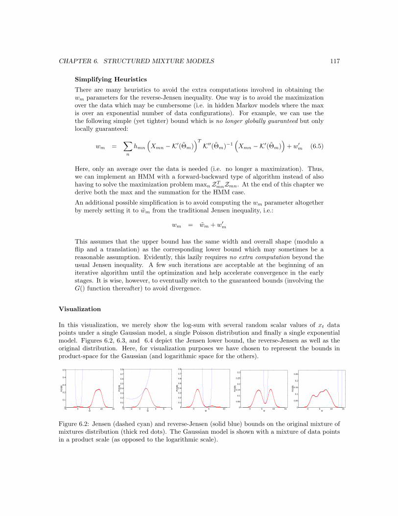
CHAPTER 6. STRUCTURED MIXTURE MODELS 117
Simplifying Heuristics
There are many heuristics to avoid the extra computations involved in obtaining thewm parameters for the reverse-Jensen inequality. One way is to avoid the maximizationover the data which may be cumbersome (i.e. in hidden Markov models where the maxis over an exponential number of data configurations). For example, we can use thethe following simple (yet tighter) bound which is no longer globally guaranteed but onlylocally guaranteed:
wm =∑
n
hmn
(Xmn −K′(Θm)
)T
K′′(Θm)−1(Xmn −K′(Θm)
)+ w′m (6.5)
Here, only an average over the data is needed (i.e. no longer a maximization). Thus,we can implement an HMM with a forward-backward type of algorithm instead of alsohaving to solve the maximization problem maxnZT
mnZmn. At the end of this chapter wederive both the max and the summation for the HMM case.
An additional possible simplification is to avoid computing the wm parameter altogetherby merely setting it to wm from the traditional Jensen inequality, i.e.:
wm = wm + w′m
This assumes that the upper bound has the same width and overall shape (modulo aflip and a translation) as the corresponding lower bound which may sometimes be areasonable assumption. Evidently, this lazily requires no extra computation beyond theusual Jensen inequality. A few such iterations are acceptable at the beginning of aniterative algorithm until the optimization and help accelerate convergence in the earlystages. It is wise, however, to eventually switch to the guaranteed bounds (involving theG() function thereafter) to avoid divergence.
Visualization
In this visualization, we merely show the log-sum with several random scalar values of xt datapoints under a single Gaussian model, a single Poisson distribution and finally a single exponentialmodel. Figures 6.2, 6.3, and 6.4 depict the Jensen lower bound, the reverse-Jensen as well as theoriginal distribution. Here, for visualization purposes we have chosen to represent the bounds inproduct-space for the Gaussian (and logarithmic space for the others).
−5 0 5 10 150
0.1
0.2
0.3
0.4
0.5
Θ
P(X
|Θ)
−4 −2 0 2 4 6 80
0.1
0.2
0.3
0.4
0.5
0.6
0.7
0.8
Θ
P(X
|Θ)
0 5 100
0.1
0.2
0.3
0.4
0.5
0.6
0.7
0.8
Θ
P(X
|Θ)
0 5 10 150
0.05
0.1
0.15
0.2
0.25
0.3
Θ
P(X
|Θ)
0 5 10 150
0.05
0.1
0.15
0.2
0.25
Θ
P(X
|Θ)
Figure 6.2: Jensen (dashed cyan) and reverse-Jensen (solid blue) bounds on the original mixture ofmixtures distribution (thick red dots). The Gaussian model is shown with a mixture of data pointsin a product scale (as opposed to the logarithmic scale).
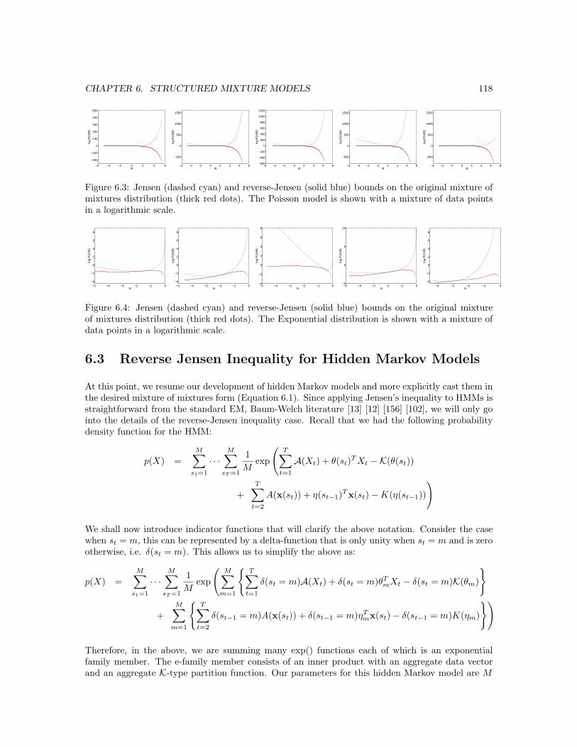
CHAPTER 6. STRUCTURED MIXTURE MODELS 118
−6 −4 −2 0 2 4 6
−200
−100
0
100
200
300
400
500
Θ
log
P(X
|Θ)
−6 −4 −2 0 2 4 6 8
−500
0
500
1000
1500
Θlo
g P
(X|Θ
)
−6 −4 −2 0 2 4 6 8−600
−400
−200
0
200
400
600
800
1000
1200
Θ
log
P(X
|Θ)
−6 −4 −2 0 2 4 6 8
−500
0
500
1000
1500
Θ
log
P(X
|Θ)
−6 −4 −2 0 2 4 6 8
−500
0
500
1000
1500
Θ
log
P(X
|Θ)
Figure 6.3: Jensen (dashed cyan) and reverse-Jensen (solid blue) bounds on the original mixture ofmixtures distribution (thick red dots). The Poisson model is shown with a mixture of data pointsin a logarithmic scale.
−5 −4 −3 −2 −1 0−4
−2
0
2
4
6
8
Θ
log
P(X
|Θ)
−5 −4 −3 −2 −1 0−4
−2
0
2
4
6
8
Θ
log
P(X
|Θ)
−5 −4 −3 −2 −1 0−4
−2
0
2
4
6
8
Θ
log
P(X
|Θ)
−5 −4 −3 −2 −1 0−5
0
5
10
Θ
log
P(X
|Θ)
−4 −3 −2 −1 0−4
−2
0
2
4
6
8
Θ
log
P(X
|Θ)
Figure 6.4: Jensen (dashed cyan) and reverse-Jensen (solid blue) bounds on the original mixtureof mixtures distribution (thick red dots). The Exponential distribution is shown with a mixture ofdata points in a logarithmic scale.
6.3 Reverse Jensen Inequality for Hidden Markov Models
At this point, we resume our development of hidden Markov models and more explicitly cast them inthe desired mixture of mixtures form (Equation 6.1). Since applying Jensen’s inequality to HMMs isstraightforward from the standard EM, Baum-Welch literature [13] [12] [156] [102], we will only gointo the details of the reverse-Jensen inequality case. Recall that we had the following probabilitydensity function for the HMM:
p(X) =M∑
s1=1
· · ·M∑
sT =1
1M
exp
(T∑
t=1
A(Xt) + θ(st)T Xt −K(θ(st))
+T∑
t=2
A(x(st)) + η(st−1)T x(st)−K(η(st−1))
)
We shall now introduce indicator functions that will clarify the above notation. Consider the casewhen st = m, this can be represented by a delta-function that is only unity when st = m and is zerootherwise, i.e. δ(st = m). This allows us to simplify the above as:
p(X) =M∑
s1=1
· · ·M∑
sT =1
1M
exp
(M∑
m=1
{T∑
t=1
δ(st = m)A(Xt) + δ(st = m)θTmXt − δ(st = m)K(θm)
}
+M∑
m=1
{T∑
t=2
δ(st−1 = m)A(x(st)) + δ(st−1 = m)ηTmx(st)− δ(st−1 = m)K(ηm)
})
Therefore, in the above, we are summing many exp() functions each of which is an exponentialfamily member. The e-family member consists of an inner product with an aggregate data vectorand an aggregate K-type partition function. Our parameters for this hidden Markov model are M
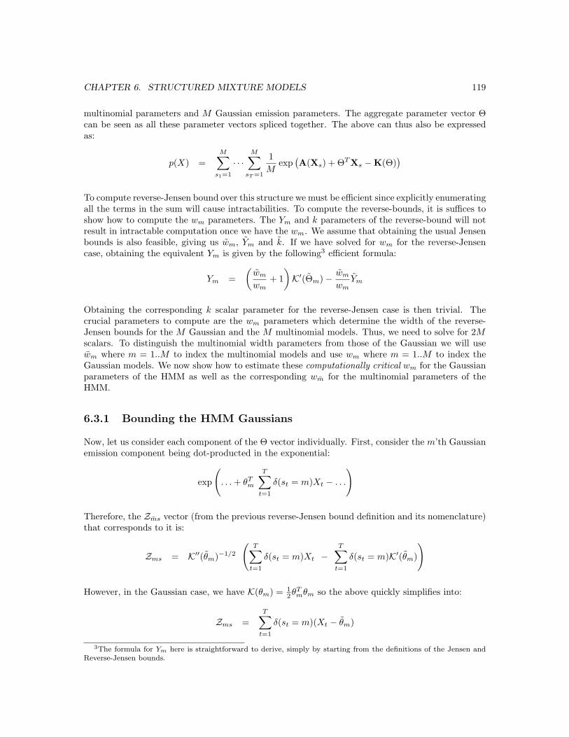
CHAPTER 6. STRUCTURED MIXTURE MODELS 119
multinomial parameters and M Gaussian emission parameters. The aggregate parameter vector Θcan be seen as all these parameter vectors spliced together. The above can thus also be expressedas:
p(X) =M∑
s1=1
· · ·M∑
sT =1
1M
exp(A(Xs) + ΘT Xs −K(Θ)
)To compute reverse-Jensen bound over this structure we must be efficient since explicitly enumeratingall the terms in the sum will cause intractabilities. To compute the reverse-bounds, it is suffices toshow how to compute the wm parameters. The Ym and k parameters of the reverse-bound will notresult in intractable computation once we have the wm. We assume that obtaining the usual Jensenbounds is also feasible, giving us wm, Ym and k. If we have solved for wm for the reverse-Jensencase, obtaining the equivalent Ym is given by the following3 efficient formula:
Ym =(
wm
wm+ 1)K′(Θm)− wm
wmYm
Obtaining the corresponding k scalar parameter for the reverse-Jensen case is then trivial. Thecrucial parameters to compute are the wm parameters which determine the width of the reverse-Jensen bounds for the M Gaussian and the M multinomial models. Thus, we need to solve for 2Mscalars. To distinguish the multinomial width parameters from those of the Gaussian we will usewm where m = 1..M to index the multinomial models and use wm where m = 1..M to index theGaussian models. We now show how to estimate these computationally critical wm for the Gaussianparameters of the HMM as well as the corresponding wm for the multinomial parameters of theHMM.
6.3.1 Bounding the HMM Gaussians
Now, let us consider each component of the Θ vector individually. First, consider the m’th Gaussianemission component being dot-producted in the exponential:
exp
(. . . + θT
m
T∑t=1
δ(st = m)Xt − . . .
)
Therefore, the Zms vector (from the previous reverse-Jensen bound definition and its nomenclature)that corresponds to it is:
Zms = K′′(θm)−1/2
(T∑
t=1
δ(st = m)Xt −T∑
t=1
δ(st = m)K′(θm)
)
However, in the Gaussian case, we have K(θm) = 12θT
mθm so the above quickly simplifies into:
Zms =T∑
t=1
δ(st = m)(Xt − θm)
3The formula for Ym here is straightforward to derive, simply by starting from the definitions of the Jensen andReverse-Jensen bounds.

CHAPTER 6. STRUCTURED MIXTURE MODELS 120
Now, to compute the wm (and later the wm for the multinomial) that correspond to the necessaryreverse-Jensen bounds we need to efficiently evaluate the following expressions or upper bounds onthem: ∑
s
hsZTmsZms
maxsZT
msZms
Above we recognize the responsibility terms hs which are the probability posteriors over the latentstate paths at the previous model setting Θ given the observations {X} or X1, . . . , XT . Thus, theycan be written as hs = p(s1, . . . , sT |{X}, Θ). Let us now expand out the required the inner productsin the above computations:
ZTmsZms =
T∑t=1
δ(st = m)(Xt − θm)T ×T∑
t=1
δ(st = m)(Xt − θm)
For one of the terms of the reverse-Jensen bound, we need the max over all such possible innerproducts. Thus we need compute the maximum over any path of the above quantity:
maxsZT
msZms = maxs
T∑t=1
δ(st = m)(Xt − θm)T ×T∑
τ=1
δ(sτ = m)(Xτ − θm)
Expanding the above, we obtain:
maxsZT
msZms = maxs
T∑t=1
T∑τ=1
δ(st = m)δ(sτ = m)(Xt − θm)T (Xτ − θm)
The discrete optimization required now will probably require integer programming to solve exactly(probably some variant of the knapsack problem). However, we can find an upper bound on thedesired quantity with a simple a quadratic program. To do so, we simply introduce the followingλ-scalar variables:
λt := δ(st = m)
We do this for all time steps t ∈ [1, . . . , T ]. These λt are bounded over λt ∈ [0, 1] and thus are asuper-set of the binary variables. Therefore, maximizing over this larger space of variables will yieldthe true maxsZT
msZms or an upper bound over it. Thus, we can replace the above optimizationwith:
maxsZT
msZms ≤ maxλ1,...,λT
T∑t=1
T∑τ=1
λtλτ (Xt − θm)T (Xτ − θm) ∀λt ∈ [0, 1]
The above is a quadratic program over T variables with 2T inequality constraints which can besolved in a straightforward manner (subject to the box constraints on λt ∈ [0, 1]). It is also evidentthat the maximum usually lies outside the convex hull of constraints and will typically cause the λt
to rail to their extremes at the end of the optimization (except for degenerate situations). Therefore,we get a more conservative value for the maximum data magnitude which is still a guaranteed upperbound.

CHAPTER 6. STRUCTURED MIXTURE MODELS 121
Now, we detail the computation of the other component of the wm bound-parameter: the ’expectedmagnitude’ (instead of the max):
∑s
hsZTmsZms =
∑s
hs
T∑t=1
δ(st = m)(Xt − θm)T ×T∑
t=1
δ(st = m)(Xt − θm)
Expanding the above, we obtain:
∑s
hsZTmsZms =
T∑t=1
T∑τ=1
(∑s
hsδ(st = m)δ(sτ = m)
)(Xt − θm)T (Xτ − θm)
=T∑
t=1
T∑τ=1
p(st = m, sτ = m|{X}, Θ) (Xt − θm)T (Xτ − θm)
In the above, we have introduced the marginal distribution p(st = m, sτ = m|{X}, Θ) over the stateat time t being m and the state at time τ being m after the HMM observations have been accountedfor. This marginal distribution over a state sequence sub-string is straightforward to computeefficiently since the HMM is a tree-structured graphical model which permits efficient computationof marginal distributions (which is based on the Baum-Welch forward backward algorithm). In thecase where τ = t, the probability is merely p(st = m|{X}, Θ) which is equal to the traditionalnormalized αt(m)βt(m) product from the familiar forward-backward algorithm [156].
For completeness, we will show how to compute the marginal distribution p(st, sτ |{X}),where we will assume, without loss of generality, that t < τ . Several quantities areeasy to compute after the forward-backward algorithm. Once of them is the marginalover a single state: p(st|{X}) = αtβt. Similarly, there is a direct formula for themarginal over a pair of subsequent states (where ct is Rabiner’s so-called scaling factor):p(st+1, st|{X}) = ct+1α(st)p(st+1|st)p(Xt+1|st+1)β(st+1). Using Bayes’ rule gives condi-tionals on pairs of subsequent states p(st+2|st+1, {X}) = p(st+2, st+1|{X})/p(st+1|{X}).Thus, we can obtain the following three-way marginal by multiplying a pairwise marginalwith a conditional: p(st+2, st+1, st|{X}) = p(st+2|st+1, {X})p(st+1, st|{X}). To obtainp(st+2, st|{X}) we merely sum the later marginal over st+1. This reasonably efficientprocess is iterated until we reach p(st, sτ |{X}) and does not require intractable compu-tation.
The above computation can be implemented efficiently with approximately O(T 2M2) operationssince we need to consider bivariate probability distributions p(st, sτ ) which are of order M ×M forevery pair of time points in the trellis of length T . Although this is a factor of T slower than thecomputation of the forward backward algorithm in regular hidden Markov models which is typicallyO(TM2), the above computation is tractable (particularly for short trellis lengths).
The computations outlined thus readily give us both components (or legitimate upper bounds onthem) of the wm bound parameter efficiently without doing intractable calculations. These onlyrequire a simple quadratic program as well as the results from EM’s Baum-Welch computations. Wenow move to bounding the multinomial parameters.

CHAPTER 6. STRUCTURED MIXTURE MODELS 122
6.3.2 Bounding the HMM Multinomials
Next consider the m’th multinomial component which is being dot-producted inside the exponentialfunction as follows:
exp
(. . . + ηT
m
T∑t=2
δ(st−1 = m)x(st)− . . .
)
Therefore, the Zms vector (from the previous reverse-Jensen bound nomenclature) that correspondsto it is:
Zms = K ′′(ηm)−1/2
(T∑
t=2
δ(st−1 = m)x(st) −T∑
t=2
δ(st−1 = m)K ′(ηm)
)
=T∑
t=2
δ(st−1 = m) K ′′(ηm)−1/2 (x(st) − K ′(ηm))
Now, to compute the wm that correspond to the necessary reverse-Jensen bounds, we need toefficiently evaluate the following: ∑
s
hsZTmsZms
maxsZT
msZms
As before, we can expand the inner products as follows:
ZTmsZms =
T∑t=2
T∑τ=2
δ(st−1 = m)δ(sτ−1 = m) (x(st) − K ′(ηm))TK ′′(ηm)−1 (x(sτ ) − K ′(ηm))
Since the x data here correspond to only a choice of one of the M -multinomial models, we canrewrite it as follows:
x(st) =M∑
q=1
δ(st = q)xq
For notational convenience, we also define the following:
zq = K ′′(ηm)−1/2 (xq −K ′(ηm))
Thus, the desired inner product term becomes:
ZTmsZms =
T∑t=2
T∑τ=2
δ(st−1 = m)δ(sτ−1 = m)
(M∑
q=1
zqδ(st = q)
)T ( M∑r=1
zrδ(sτ = r)
)
=T∑
t=2
T∑τ=2
δ(st−1 = m)δ(sτ−1 = m)
(M∑
q=1
M∑r=1
δ(st = q)δ(sτ = r)zTq zr
)
To obtain the desired wm reverse-Jensen bound parameter for the multinomials, we need to computetwo terms using the above inner-products. These are the expected term (the sum over all the inner

CHAPTER 6. STRUCTURED MIXTURE MODELS 123
products weighted by the hs probabilities) and the max type term. The maxs term is elucidatedfirst:
maxsZT
msZms = maxs
M∑q=1
M∑r=1
T∑t=2
T∑τ=2
δ(st−1 = m)δ(sτ−1 = m)δ(st = q)δ(sτ = r) zTq zr
Although an integer programming solution may be possible for the above maximization, we caninstead solve for an upper bound on it (which will still produce a guaranteed bound) by reformulatingit as follows. We first define scalars as follows:
λrq :=T∑
t=2
T∑τ=2
δ(st−1 = m)δ(sτ−1 = m)δ(st = q)δ(sτ = r)
It is clear that these scalars are all positive, i.e. λrq ≥ 0 which gives us M2 constraints. Furthermore,we have the following constraint on these variables:∑
r
∑q
λrq ≤ (T − 1)2
Therefore we can solve for an upper bound on the desired quantity via a simple linear programover the M2 surrogate variables λrq. By allowing these surrogate λ variables to vary as continuousparameters over the constrained range, we are solving for a more flexible maximization than theoriginal integer programming problem over state paths. Therefore optimizing over the λ will yield amore conservative upper bound on the quantity of interest (which still produces a legitimate reverse-Jensen bound overall). The solution can thus be solve via the simple linear form below (with thecorresponding M2 + 1 inequality constraints imposed on the λ-variables):
maxsZT
msZms ≤ maxλ
M∑q=1
M∑r=1
λrq zTq zr
Now, we turn our attention to the computation of the expected inner product (versus the maximum):
∑s
hsZTmsZms =
∑s
hs
M∑q=1
M∑r=1
T∑t=2
T∑τ=2
δ(st−1 = m)δ(sτ−1 = m)δ(st = q)δ(sτ = r) zTq zr
=M∑
q=1
M∑r=1
T∑t=2
T∑τ=2
∑s
hsδ(st−1 = m)δ(sτ−1 = m)δ(st = q)δ(sτ = r) zTq zr
=M∑
q=1
M∑r=1
T∑t=2
T∑τ=2
p(st−1 = m, sτ−1 = m, st = q, sτ = r|{X}, Θ) zTq zr
Once again we have to simply use the marginal distribution over a state sub-string p(st−1 =m, sτ−1 = m, st = q, sτ = r|{X}, Θ) which is readily obtainable for a tree-structure or chainstructure HMM model without intractable computation. The clique size being considered is over 4variables here which leads to more work then in a standard EM setting, it appears that computingthe expected data magnitude as opposed to expected data vectors (as EM does) requires squaredclique sizes. More specifically, the implementation of the above requires O(T 2M4) operations sincewe need to consider 4-variable probability distributions p(st, st−1, sτ , sτ−1) which are of order M4

CHAPTER 6. STRUCTURED MIXTURE MODELS 124
for every pair of time points in the trellis of length T . Although this is slower than the computationof the forward backward algorithm in a regular hidden Markov model (which is typically O(TM2))the above computation is still tractable.
The above computations thus give us both the wm and the wm parameters for the Gaussian and theMultinomial components of the reverse-Jensen bound without resorting to intractable computation.All computations remain efficient via appeals to linear programming, quadratic programming andforward-backward types of dynamic programming.
6.4 Conditional Hidden Markov Models
Given both Jensen and reverse-Jensen bounds for hidden Markov models, it is now feasible to usethe CEM algorithm and perform conditional likelihood maximization in a straightforward way. Inthis section, we will describe one scenario where it becomes necessary to optimize a conditionallikelihood quantity. There are many other situations where a conditional expression will arise dueto the problem formulation and result in a negated log-sum type of expression. Negated log-sumsand conditional likelihood expressions would occur, for example, when learning a classifier basedon multiple competing hidden Markov models, or when learning a mixture-of-experts regressionfunction whose gates are hidden Markov models. In this section we will focus on and develop whatis traditionally called an input-output hidden Markov model [16] where the objective is to regresscertain components of a time series from others which are observable. Both inputs and outputs arecoupled through a hidden state which evolves with Markov dynamics.
We begin with a standard hidden Markov model as portrayed in the previous sections and assumethat we are given a time sequence of vectors. For an input-output hidden Markov model, we splitthe emission vectors into two components: x and y which are to be treated as input and outputrespectively. Given a training sequence of such x1, . . . , xT and y1, . . . , yT vector-pairs over time, wewould like to estimate a hidden Markov model such that, on future test data, we can reliably predicta y1, . . . , yτ sequence from a given x1, . . . , xτ sequence alone. An example application would be tolearn the mapping from various passive biological measurements such as heart-rate, temperature,motion energy, etc. to a more complicate output measurement such as blood-glucose which wouldnot always be easily measurable.
We shall assume that we are dealing with an HMM with a total of M underlying states whichgives rise to an M ×M transition matrix. This transition matrix is equivalently described by Mmultinomial distributions of dimensionality equal to M . We will further assume that the emissionmodel for x and y is jointly Gaussian with a diagonal covariance matrix. Therefore, it is necessaryto estimate the M Gaussian covariance terms, the M Gaussian mean terms and the M ×M statetransition matrix.
Since we wish to regress y from x, it is natural to form a conditional distribution of p(y|x) and anatural objective function is the conditional log-likelihood on the training data below:
lc = log p(x, y)− log p(x)
We can view the first term in the above expression as the log-likelihood of the whole hidden Markovmodel on the training data. The second (negated) term, is the likelihood of the hidden Markovmodel after it has been marginalized and only applies the input data x. Figuratively, we have thefollowing graphical model scenario:
Recall that p(x, y) and p(x) in the above expressions are latent quantities which involve a summationover all possible paths in the state space of the hidden Markov model. In other words, we can expand
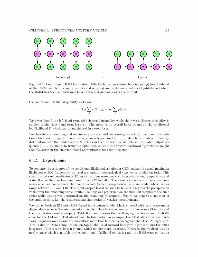
CHAPTER 6. STRUCTURED MIXTURE MODELS 125
S1 S2 S3 S4 S5
Y1 Y2 Y3 Y4 Y5
X1 X2 X3 X4 X5
S1 S2 S3 S4 S5
X1 X2 X3 X4 X5
log p(x, y) − log p(x)
Figure 6.5: Conditional HMM Estimation. Effectively, we maximize the joint p(x, y) log-likelihoodof the HMM over both x and y (inputs and outputs) minus the marginal p(x) log-likelihood wherethe HMM has been summed over to obtain a marginal only over the x input.
the conditional likelihood quantity as follows.
lc = log∑S
p(S, x, y)− log∑S
p(S, x)
We lower bound the left hand term with Jensen’s inequality while the reverse-Jensen inequality isapplied to the right hand term log p(x). This gives us an overall lower bound on the conditionallog-likelihood lc which can be maximized in closed form.
We then iterate bounding and maximization steps until we converge to a local maximum of condi-tional likelihood. To perform regression, we merely use novel x1, . . . , xτ data to estimate a probabilitydistribution over the hidden states S. This can then be used to compute an estimated output se-quence y1, . . . , yτ simply by using the alpha-beta values in the forward-backward algorithm to weighteach Gaussian in the emission model appropriately for each time step.
6.4.1 Experiments
To compare the estimates of the conditional likelihood criterion or CEM against the usual maximumlikelihood or EM framework, we used a standard meteorological time series prediction task. Thissmall toy data set constitutes of 420 monthly of measurements of the precipitation, temperature andwater flow in the San Francisco area from 1932 to 1966. Therefore, we have a 4 dimensional timeseries when we concatenate the month as well (which is represented as a sinusoidal whose valuesrange between -1.0 and 1.0). The input-output HMM we wish to build will regress the precipitationvalue from the remaining three inputs. Training was performed on the first 360 samples of the timeseries while testing was performed on the remaining 60 samples. Figure 6.6 depicts a snapshot ofthe training data, i.e. the 4-dimensional time series of weather measurements.
We trained both an EM and a CEM based input-output hidden Markov model with 4 states assumingdiagonal-covariance Gaussian emission models. The Gaussians are over 4 dimensions (3 inputs andthe precipitation level as output). Table 6.4.1 summarizes the resulting log likelihoods and the RMSerror for the EM and CEM algorithms. In this particular example, the CEM algorithm was muchslower requiring over 2 orders of magnitude more time to attain convergence than the EM algorithm.This is due to extra computations on top of the usual forward-backward algorithm and the extralooseness of the reverse-Jensen bounds which require more iterations. However, the resulting testingperformance which is notable in the conditional likelihood on testing and the RMS error on testing

CHAPTER 6. STRUCTURED MIXTURE MODELS 126
0 20 40 60 80 100−20
0
20
40
60
80
100
120
Month
Mon
th, T
emp,
Flo
w, P
reci
p
Figure 6.6: Training data from the San Francisco Data Set. Here, the 4-dimensional time seriesdepicts the monthly levels of precipitation, water flow, temperature as well as the month of year asa sinusoid.
shows CEM performed favorably when compared to EM based prediction. For an appropriate andquantitative measure of performance, the conditional likelihood on testing data is the best choicesince the given task here is to predict precipitation values from the other inputs. Therefore, it isinappropriate to penalize or reward good estimates of the input components. Thus joint likelihoodon test data is an inappropriate measurement of the quality of the estimate. Only the desiredoutputs need to be properly predicted and hence the conditional likelihood score (as well as RMSerror) depict that a better regression estimate is obtained by the CEM algorithm.
Training Log-Likelihood Conditional Log-LikelihoodEM -5.985 -3.473CEM -9.683 -3.066Testing Log-Likelihood Conditional Log-Likelihood RMS ErrorEM -6.466 -3.463 195.2CEM -9.360 -3.110 184.6
Table 6.1: CEM & EM Performance for HMM Precipitation Prediction.
Figure 6.7 shows a qualitative performance difference between the EM-based hidden Markov modeland the CEM-based hidden Markov model. Note how the CEM version tracks the precipitationvalues (during testing) more closely than the EM and also has a more accurate range of variationthan the conservative near-constant precipitation estimates EM generates.
In Chapter 8, a more ambitious application of the input-output HMM regression will be attempted.However, due to the extremely large size of the data and its long trellis length, simplifying approxi-mations will be needed to reduce the computation time of the CEM algorithm such that it operatesin roughly the same time as the EM algorithm.
6.5 Discriminative Hidden Markov Models
In this section we will give details of an implementation of MED for hidden Markov models in adiscriminative regression setting. Unlike the standard regression or conditional regression in theprevious input-output HMM, we will here use a discriminative epsilon-tube insensitivity with linearloss function to form the regression function. The implementation for a classification setting is

CHAPTER 6. STRUCTURED MIXTURE MODELS 127
360 370 380 390 400 410 4200
20
40
60
80
100
120
Month
Pre
cipi
tatio
n
Figure 6.7: Test predictions for the San Francisco Data Set. The true precipitation values aredepicted with the dashed cyan line and the filled dots. The EM hidden Markov model’s predictionsare outlined with the dashed red line connecting the ’x’ points. The CEM hidden Markov model’spredictions are outlined by the solid blue line connecting the hollow ’o’ circles. Note how the CEMpredictions track the true precipitation values more closely while the EM predictions do not spanthe desired range of variation and do not align well with the desired output.
straightforward given the regression development here. While classification has many applications(i.e. speech recognition, bioinformatics, etc.) we will portray the discriminative regression HMMas a novel way to incorporate time invariance in regression settings. Recall in section 4.1 where wedeveloped MED for regression applications and discussed the use of generative and latent generativemodels therein. We now consider the following regression discriminant function:
L(X; Θ) = log∑
S p(X, S|θ+)∑S p(X, S|θ−)
+ b
Where the numerator and denominator are hidden Markov models which define a probability densityover each X datum which is itself a sequence of observations instead of a single vector. Recall theregression constraints that arise in the MED framework:∫
P (Θ, γ) [yt − L(Xt; Θ) + γt] dΘdγ ≥ 0, t = 1..T∫P (Θ, γ) [γ′t − yt + L(Xt; Θ)] dΘdγ ≥ 0, t = 1..T
The expectations over the discriminant functions above are intractable and therefore we will employvariational bounds instead (Jensen and reverse-Jensen). In the first constraint, we will need toupper bound L(Xt; Θ) while in the second constraint we will need to lower bound L(Xt; Θ). This willresult in the creation of more restrictive constraints that generate a convex hull that is containedin the convex hull of the original MED problem. In the first set of constraints, we will use reverse-Jensen on the numerator and the Jensen bound on the denominator. The situation is reversed forthe other set of constraints. Once the variational bounds are used, the MED solution distributionP (Θ) will factorize across all the (positive and negative) HMM parameters (i.e. the emissions andtransitions) if our prior over these P0(Θ) is conjugate and factorized itself. Assume we have invokedthe inequalities at a given Θ operating point and now have the following constraints instead:∫
P (Θ, γ)
[yt +
∑m
wtm log p(Ytm|m, θ+)− kt +∑m
wtm log p(Ytm|m, θ−) + kt − b + γt
]dΘdγ ≥ 0
∫P (Θ, γ)
[γ′t − yt +
∑m
wtm log p(Ytm|m, θ+) + kt +∑m
wtm log p(Ytm|m, θ−)− kt + b
]dΘdγ ≥ 0

CHAPTER 6. STRUCTURED MIXTURE MODELS 128
In the above, we have used Jensen and reverse-Jensen on each training sequence Xt in the datat = 1..T to obtain the parameters of the bounds: wtm, Ytm, kt and wtm, Ytm, kt for each HMMmodel (both the positive and the negative one). Here, m indexes over the M Gaussian emissionmodels and the M multinomial (transition matrix) models for each HMM respectively. To computethe bounds we convert the multinomial in natural parameterization for the Jensen/reverse-Jensencomputations and back to the form in section 3.9.4 for the MED computations. The Gaussian isonly over means and therefore is always in its natural parameterization. The above constraints giverise to the following partition function where the margin (with exponential prior) and bias (withGaussian prior) components are the same as any simple (linear) MED regression:
Z(λ) = Zγ(λ) Zb(λ) Zθ+(λ) Zθ−(λ)
The only novel computation involves solving for the Zθ+ and Zθ− components since the other com-ponents were already explored in previous regression problems. A closed form partition function isneeded so that we can estimate the optimal setting of the Lagrange multipliers. Each of the mod-els, θ+ and θ− contains the M Gaussian emission parameters and M multinomial parameters of thepositive (numerator) HMM. We will assume white Gaussian priors over the emission parameters anduniform Dirichlet priors (i.e. αk = α = 1/M in the notation of section 3.9.4) over the multinomials.It suffices to show how to compute the partition function component for one of the HMMs, say Zθ+ ,which is given by:
Zθ+(λ) =∫
θ+
P0(θ+)e∑
tλt
∑m
wtm log p(Ytm|m,θ+)−λtkt+∑
tλ′t∑
mwtm log p(Ytm|m,θ+)+λ′tktdθ+
The above partition function component can be further broken down as follows:
Zθ+(λ) = Zlinear+(λ) × ΠMn=1Zgauss+,n(λ) × ΠM
q=1Zmulti+,q(λ)
There is a simple log-linear component which is given by the following:
Zlinear+(λ) = e−∑
tλtkt+
∑t
λ′tkt
There are n = 1..M Gaussian partition function components given here in logarithmic form (wherethe A(Y ) = −1/2Y T Y −D/2 log(2π), as usual for a Gaussian e-family model):
log Zgauss+,n(λ) = log∫
P0(µn)e∑
tλtwtn(A(Ytn)+Y T
tnµn−1/2µTn µn)+
∑t
λ′twtn(A(Ytn)+Y Ttnµn−1/2µT
n µn)dµn
log Zgauss+,n(λ) =∑
t
λtwtnA(Ytn) +∑
t
λ′twtnA(Ytn)− 12
log
(1 +
∑t
λtwtn +∑
t
λ′twtn
)
+12
(∑t λtwtnYtn +
∑t λ′twtnYtn
)T (∑t λtwtnYtn +
∑t λ′twtnYtn
)1 +
∑t λtwtn +
∑t λ′twtn
We also have to consider the contribution of the q = 1..M multinomial components. We first convertthe natural parameterization of the data, i.e. the M − 1-dimensional vectors Ytq, into the standardmultinomial form with M -dimensional vectors Utq. This is done by concatenating an extra elementto the vector such that it sums to unity. We then integrate to obtain the following partition functionwhich is reminiscent of the derivation in Section 3.9.4 (and we use the superscript k to index intothe dimensionality of the Utq vectors):
Zmulti+,q ∝ΠM
k=1Γ(αk +∑
t λtwtqUktq +
∑t λ′twtqU
ktq)
Γ(∑M
k=1 αk +∑
t λtwtqUktq +
∑t λ′twtqUk
tq)e
∑t
λtwtq
Γ(1+∑M
k=1Uk
tq)
ΠMk=1
Γ(1+Uktq
)+∑
tλ′twtq
Γ(1+∑M
k=1Uk
tq)
ΠMk=1
Γ(1+Uktq
)

CHAPTER 6. STRUCTURED MIXTURE MODELS 129
For computing the partition function for the negative HMM, we merely use its own Jensen andreverse-Jensen parameters and permute the roles of λ and λ′. The negative of the logarithm of theaggregate partition function is then maximized. There are redundancies in the above computationsand they are all computable efficiently if only a single Lagrange multiplier is modified at a time.This permits a fast axis-parallel implementation.
Once we have sufficiently optimized over the Lagrange multipliers, we can use the current settingof these to compute P (Θ). To obtain the next Θ setting, we merely find the maximum of P (Θ).For the Gaussian models, the maximum is merely at the mean which involves the following simpleupdate rule (the negative model’s parameters are updated similarly with their bounds and the roleof the λt and λ′t swapped):
µn+ =∑
t λtwtnYtn +∑
t λ′twtnYtn
1 +∑
t λtwtn +∑
t λ′twtn
For the q’th multinomial, the natural parameters are θ+q which permit a simple update rule involvingthe gradients of the cumulant-generating function K = log(1+
∑i exp(θi)). The following rule merely
finds the max of the MED solution distribution P (θ+q) in e-family form (the ~1 is used to denote avector of ones of the same size as Ytq):
∂K(θ+q)∂θ+q
=α~1 +
∑t λtwtqYtq +
∑t λ′twtqYtq
1 +∑
t λtwtq +∑
t λ′twtq
Once the max has been found, we can re-convert the natural representation of θ+q back into theusual multinomial parameterization (using ρ as in Section 3.9.4). Thus, we iterate, updating the Θcontact point, recomputing the bounds, and estimating the Lagrange multipliers. This is continueduntil convergence (a heuristic stopping criterion is used). Utilizing the MED solution P (Θ) forprediction is still intractable even after training is performed since we must compute expectationsover the HMM. Instead, during run-time, we merely use the maximum Θ = argmaxP (Θ) whichgives us two fixed HMM models. The log-ratio of their likelihoods (with the bias scalar parameter)is then used to compute the regression to obtain an approximate output:
y =∫
P (Θ)L(X; Θ)dΘ
y ≈ L(X; Θ)
We can thus form a discriminative regression model that inherits the dynamic-time-warping proper-ties of an HMM while optimizing an epsilon-tube insensitive scalar prediction. The above expressionscan be trivially re-applied to also create discriminative HMMs for classification where the parametersof each HMM are estimated such that we obtain a large-margin decision boundary between the twogenerative models (unlike in the standard maximum-likelihood setting).
6.6 Latent Bayesian Networks
We shall now discuss the case of Bayesian networks in general, of which hidden Markov models area specific example. The hidden Markov model has a chain dependency structure which maintainssome important computational properties that were useful for computing Jensen and reverse-Jensenbounds efficiently. It is well known that Bayesian networks which have tree structures can alsotake advantage of efficient algorithms to avoid intractabilities and therefore may also be possible to

CHAPTER 6. STRUCTURED MIXTURE MODELS 130
estimate discriminatively (with the Jensen and reverse-Jensen bounds). Recall that tree structureddependencies between variables who are themselves in the exponential family form an aggregateexponential-family distribution [34]. Now, if we have latent or hidden variables in the Bayes netgraph, these tree structures need to be summed over. Therefore, the log-likelihood of the latent Bayesnet can be represented as a mixture of exponential family distributions. Again, this can be writtenin the mixture of mixtures form of Equation 6.1. Subsequently, its logarithm (the log-likelihood ofthe latent Bayes net) can be upper and lower bounded via Jensen and reverse-Jensen. Although wecan compute these bounds merely by unfolding the latencies in the mixture of mixtures, this may behighly inefficient. The computations for the wm would become intractable since they would requireenumerating all latent configurations in the Bayesian networks. Just as we demonstrated for thehidden Markov model where efficient algorithms avoid the exponentially large explicit mixture model,we need an efficient algorithm to compute the reverse-Jensen bounds for general tree-structuredBayes nets by taking advantage of the conditional independency properties of the graphical model.Otherwise, naive computation of Jensen and reverse-Jensen bounds will require intractable amountsof work for latent Bayesian networks.
It is possible to compute lower bounds efficiently by taking advantage of the independency structurein the networks and that is done for the regular Jensen inequality parameters by using EM and theso-called Junction Tree Algorithm [102]. In fact, the forward-backward algorithm that we modifiedfor the reverse-Jensen bound is a special case of the more general junction-tree algorithm. Both aremethods that take advantage of the structure of the graph to efficiently compute expectations. Forsolving the reverse-Jensen upper bound’s parameters, we also need such efficient procedures thattake advantage of the graph structure. Just as was shown for the HMM, the general case of latenttree-structured Bayesian networks may also have a similar efficient reverse-Jensen algorithms andthis direction definitely merits further investigation.
6.7 Data Set Bounds
So far, we have considered only bounds (lower and upper) on the log-likelihood of a single data pointor single sequence (in the HMM case). However, it is often the case that we will want to boundthe likelihood of a data set of many points. If this is the case, the reverse-Jensen inequality can beapplied in a more straightforward way. The main benefit is that the reverse-Jensen inequality willbe applied once to form the bound instead of being applied separately for each data point and thismay generate a more efficient and more appropriately shaped bound.
Consider the following augmentation to the bounding of the log-sum. To obtain the aggregate dataset’s conditional likelihood, we must sum the likelihood over each data point as follows:
lc =∑
i
log∑m
p(m, ci, Xi|Θ)−∑
i
log∑m
∑c
p(m, c, Xi|Θ)
The conditional log-likelihood (lc) above can be seen as the joint log-likelihood (lj) minus themarginal log-likelihood (lm):
lc = lj − lm
Where in the above we have the joint log-likelihood:
lj =∑
i
log∑m
p(m, ci, Xi|Θ)

CHAPTER 6. STRUCTURED MIXTURE MODELS 131
We also have the negated marginal log-likelihood:
lm =∑
i
log∑m
∑c
p(m, c, Xi|Θ)
Since we want overall lower bounds on the conditional likelihood, we need to lower bound the jointlog-likelihood above and upper bound the marginal log-likelihood (since it gets negated). We canalso write the marginal log-likelihood more compactly as follows (which obscures the fact that it islatent):
lm =∑
i
log p(Xi|Θ)
We begin by adding a constant term to the marginal likelihood which has no effect on the shape ofthe bound. This is in the same spirit as the incremental likelihood derivation for EM in Bishop [20].This additive constant does not vary since it is based on the fixed previous Θ parameter values (i.e.at the point of tangential contact) and has no effect on the shape of the bounds:
∆lm =∑
i
logp(Xi|Θ)p(Xi|Θ)
Now, we shall do the reverse of EM and pull the summation over data into the logarithm operator.This will generate an upper bound on incremental marginal log-likelihood:∑
i
logp(Xi|Θ)p(Xi|Θ)
≤ log∑
i γip(Xi|Θ)βi∑i γip(Xi|Θ)βi
(6.6)
One thing to note in the above bound is that the γi terms can be scaled by an arbitrary amountand this will not change the shape of the bound. However, we still need to pick the γi and the βi toinsure that we have a guaranteed upper bound. These will become obvious shortly. First considerthe right hand side above and manipulate as follows:
log∑
i γip(Xi|Θ)βi∑i γip(Xi|Θ)βi
= log
∑i γip(Xi|Θ)βi × p(Xi|Θ)βi
p(Xi|Θ)βi∑j γjp(Xj |Θ)βj
log∑
i γip(Xi|Θ)βi∑i γip(Xi|Θ)βi
= log∑
i
(γip(Xi|Θ)βi∑j γjp(Xj |Θ)βi
)p(Xi|Θ)βi
p(Xi|Θ)βi
It is clear that if γi are all positive, then the terms in the parentheses are always positive and sumto unity (if we sum over the index i). Thus, due to concavity of the log() function, we can applyJensen’s inequality:
log∑
i γip(Xi|Θ)βi∑i γip(Xi|Θ)βi
≥∑
i
(γip(Xi|Θ)βi∑j γjp(Xj |Θ)βi
)log
p(Xi|Θ)βi
p(Xi|Θ)βi(6.7)
log∑
i γip(Xi|Θ)βi∑i γip(Xi|Θ)βi
≥∑
i
(γip(Xi|Θ)βi∑j γjp(Xj |Θ)βi
)βi log
p(Xi|Θ)p(Xi|Θ)
(6.8)
By inspection, we can see that Equation 6.8 is very similar to Equation 6.6 (when left and righthand sides are flipped). However, for them to be identical, we will need to guarantee that every

CHAPTER 6. STRUCTURED MIXTURE MODELS 132
term multiplying the logarithm in the right hand side of Equation 6.8 is unity. Thus we need:(γip(Xi|Θ)βi∑j γjp(Xj |Θ)βi
)βi = 1
The above can be simplified to (recall that the γi are invariant up to a global scale factor):
γi ∝ 1βip(Xi|Θ)βi
We can pick the scale factor above arbitrarily and it should be chosen for numerical precisionreasons (to avoid underflow or overflow computationally). One possible choice is to normalize theγi as follows:
γi =1
βip(Xi|Θ)βi∑j
1
βjp(Xj |Θ)βj
We should also note that the βi are always greater than or equal to unity. This is because we had:(γip(Xi|Θ)βi∑j γjp(Xj |Θ)βi
)βi = 1
Clearly, the terms in the parentheses that multiply βi are less than or equal to unity so we canconclude that βi ≥ 1.
It is evident that we have guaranteed the bound originally proposed in Equation 6.6 and we stillhave some freedom in selecting the βi (as long as they are greater than unity). We shall exploit thisfreedom to find the tightest bound possible. At this point we have the following bound:
∆lm ≤ log∑
i γip(Xi|Θ)βi∑i γip(Xi|Θ)βi
∆lm ≤ log
∑i
1βi
p(Xi|Θ)βi
p(Xi|Θ)βi∑i
1βi
The above bound holds for any distribution and for any βi that are greater than unity. However, itshould be noted that βi also sum inversely to unity since:
1βi
=γip(Xi|Θ)βi∑j γjp(Xj |Θ)βi∑
i
1βi
=∑
i
γip(Xi|Θ)βi∑j γjp(Xj |Θ)βi
= 1
Thus, we can write the bound as follows:
∆lm ≤ log
∑i
1βi
p(Xi|Θ)βi
p(Xi|Θ)βi∑i
1βi
∆lm ≤ log∑
i
1βi
(p(Xi|Θ)p(Xi|Θ)
)βi

CHAPTER 6. STRUCTURED MIXTURE MODELS 133
Expanding the above to include the latent values, we obtain:
∆lm ≤ log∑
i
1βi
(∑mc p(m, c, Xi|Θ)∑mc p(m, c, Xi|Θ)
)βi
However, the above expression is still undesirable since the power operation (i.e. ()βi) applies to amixture (over the summation over c and m). Let us consider bounding these terms to simplify themfurther. We will invoke Jensen again since the power operation (i.e. pow(., βi) or (.)βi) is a convexfunction for βi ≥ 1. This permits us to upper bound the expressions involving the power operationand thus generates an overall upper bound on ∆lm. Manipulating the mixture of terms being takento a power and applying Jensen, we obtain:(∑
mc p(m, c, Xi|Θ)∑mc p(m, c, Xi|Θ)
)βi
=
(∑mc
p(m, c, Xi|Θ)∑nd p(n, d,Xi|Θ)
)βi
(∑mc p(m, c, Xi|Θ)∑mc p(m, c, Xi|Θ)
)βi
=
(∑mc
p(m, c, Xi|Θ)∑nd p(n, d,Xi|Θ)
p(m, c, Xi|Θ)p(m, c, Xi|Θ)
)βi
(∑mc p(m, c, Xi|Θ)∑mc p(m, c, Xi|Θ)
)βi
≤∑mc
p(m, c, Xi|Θ)∑nd p(n, d, Xi|Θ)
(p(m, c, Xi|Θ)p(m, c, Xi|Θ)
)βi
It is clear that the left hand side and the right hand side are equal at the old value of Θ ensuringthat we have generated a variational bound that makes tangential contact appropriately. We cannow plug in these upper bounds on the individual terms indexed by i and get an overall stricterupper bound on ∆lm:
∆lm ≤ log∑
i
1βi
(∑mc p(m, c, Xi|Θ)∑mc p(m, c, Xi|Θ)
)βi
∆lm ≤ log∑
i
1βi
∑mc
p(m, c, Xi|Θ)∑nd p(n, d, Xi|Θ)
(p(m, c, Xi|Θ)p(m, c, Xi|Θ)
)βi
The above again holds for any arbitrary distribution as long as βi are greater than one and theirinverses sum to unity. If we more specifically assume that p(m, c, Xi|Θ) is in the exponential family,we can write it compactly as follows:
p(m, c, Xi|Θ) = αmc exp(Amc(Xi) + ΘT
mcXi −Kmc(Θmc))
In that case, the bound can be written more succinctly as:
∆lm ≤ log∑imc
1βi
p(m, c, Xi|Θ)1−βi∑nd p(n, d, Xi|Θ)
αβimc exp
(βiAmc(Xi) + βiΘT
mcXi − βiKmc(Θmc))
This bound is variational and makes contact at the old Θ configuration in the space of pdfs. Wecan now invoke the reverse-Jensen inequality on the above log-sum only one single time to obtaina bound on the whole data set. We also have the freedom of adjusting the βi (as long as they aregreater than unity and their inverses sum to unity) to ensure that this bound is as tight as possible(i.e. select the βi to minimize the resulting wm values).
CHAPTER 6. STRUCTURED MIXTURE MODELS 134
6.8 Applications
In the above we have only shown toy illustrations of the conditional hidden Markov models withCEM. Clearly, many important applications are now within reach and it would be interesting toinvestigate the performance on a real-world data set. Chapter 8 describes a behavior-imitationproblem where the hidden Markov model is used to learn how an agent interacts with the outsideworld. This is basically a stimulus-response type of model that is trained from real data by observinghuman activity for several hours. Since we only wish to predict and resynthesize the agent’s behaviorconditioned on the outside world measurements, we train the HMM with a conditional likelihoodcriterion. The imitation learning application seems well suited to the CEM algorithm and we showreal-world results using CEM instead of EM (after describing the implementation details of theexperiment). However, the next chapter, namely Chapter 7, is the derivation of the reverse-Jenseninequality which was so far put forth without proof. The mathematical reader may find the derivationinteresting while the more applied reader may wish to skip directly to Chapter 8 to see a real-worldapplication of latent discriminative learning with structured graphical models.

Chapter 7
The Reverse Jensen Inequality
Difficulties strengthen the mind, as labor does the body.
Seneca, 3 B.C. - 65 A.D.
In this chapter we shall give a terse derivation of the reverse-Jensen inequality we used in Chapter 5.The derivation is made to generate bounds that are as tight as possible and thus involves manydetails. These are shown in full to permit future extensions and tightenings. We first review someliterature in the contemporary mathematical inequalities community and show current conversesand reversals of Jensen. These do not suit the requirements of discriminative learning since thefunctional form of the bounds is not easy to combine with regular Jensen or EM-type bounds andtherefore we derive our own reversal.
7.1 Background in Inequalities and Reversals
The celebrated Jensen inequality has been formalized a century ago [99] and its roots trace evenfurther back in history. This result has been at the heart of many inequalities in statistics [40] andmathematics [150]. For example, Holder’s inequality can be easily derived from Jensen’s inequality.Jensen in its simplest form states that a convex function of an expectation is upper bounded by theexpectation of the convex function. An excellent review of Jensen’s inequality, other inequalities,convex functions and various statistical applications can be found in Pecaric et al.’s text [150].Furthermore, several converses and reversals of Jensen’s inequality are provided in the text. Some aresimple manipulations of Jensen’s inequality (i.e. assuming that the mixture is weighted by negativescalars instead of positives ones). Others refinements require further assumptions and properties onthe convex function and the elements it operates upon. Similarly, Log sum inequality and variantsof Jensen are also discussed in [40] however many of these are usually just trivial consequences ofJensen’s inequality. A more recent reversal of Jensen that has been important in statistics has beenproposed in [46]. For instance, the Jensen inequality can be reversed if the function it is appliedto has a limited range of variation or the elements it applies to are clamped to a limited domain.However, the bound proposed in [46] is fundamentally curvature based which can sometimes preventtight bounds. The uses for [46] are to find general dual-sided bounds on Csiszar Φ-divergences in
135

CHAPTER 7. THE REVERSE JENSEN INEQUALITY 136
terms of the many other divergences in the family. These permit one to map between divergences,i.e. Kullback-Leibler divergence, harmonic divergence, variational divergence, Renyi-entropy, etc.
Unfortunately, the above bounds in the literature do not directly suit our purposes. They notonly generate reversals which are not homogeneous with the regular Jensen inequality bounds (andtherefore cannot be combined easily with the EM-type bounds), but they also put requirements onthe elements in the expectation which are not appropriate for our pruposes. The elements in ourlog-sum problems are exponential family probability densities which have special properties but notnecessarily the ones explored so far in the literature. We therefore start with a blank slate and deriveour own customized reversal.
7.2 Derivation of the Reverse Jensen Inequality
We begin by recalling the inequality given without proof in the previous chapter:
log∑mn
αmn exp(Am(Xmn) + XTmnΘm −Km(Θm)) ≤
∑m
−wm(Am(Ym) + Y Tm Θm −Km(Θm)) + k
k = log p(X|Θ) +∑
m wm(Am(Ym) + Y Tm Θm −Km(Θm))
Ym = 1wm
∑n hmn
(∂Km(Θm)
∂Θm
∣∣∣Θm
−Xmn
)+ ∂Km(Θm)
∂Θm
∣∣∣Θm
w′m = minw′m such that 1w′
m
∑n hmn
(∂K(Θm)
∂Θm
∣∣∣Θm
−Xmn
)+ ∂K(Θm)
∂Θm
∣∣∣Θm
∈ ∂K(Θm)∂Θm
wm = 4 G
(∑n
hmnZTmnZmn
2 maxn ZTmnZmn
)maxnZT
mnZmn + w′m
Zmn = K′′(Θm)−1/2(Xmn −K′(Θm))hmn = αmn exp(Am(Xmn)+XT
mnΘm−Km(Θm))∑mn
αmn exp(Am(Xmn)+XTmnΘm−Km(Θm))
G(γ) =
{γ + 1
4 log(6) + 25/36log(6)2 − 1/6 γ ≥ 1/6
14 log(1/γ) + (γ−1)2
log(γ)2 γ ≤ 1/6
We will now derive the reverse-Jensen bound above in the so-called double-mixture case. Thisderivation subsumes that of the reverse-Jensen bound for the single mixture case. This derivation willfollow a somewhat general recipe for bounding quantities such as log-sums. It begins by making thevariational bound touch the original function tangentially at the current operating point. We thenfind a mapping on the non-linear K functions into a quadratic space which makes the computationstractable. The bound is then simplified by noting its convexity properties. Subsequently, we notethat a log-partition function of a Gibbs distribution arises (i.e. a log-sum of exponentiated linearterms) which needs to be bounded by a quadratic. This derivation is done in a one dimensional simplecase and then generalized by sweeping the 1d bound up to the multidimensional case. Subsequently,curvature constraints are checked on the bound which are simpler to deal with and subsume theoriginal inequality. Ultimately, a very simple formula for the bound’s parameters arises whichguarantees that it remains above the original log-sum function.
Again, we start with the log-sum which needs to be upper bounded:
log∑mn
αmn exp(Am(Xmn) + XTmnΘm −Km(Θm)) ≤
∑m
−wm(A(Ym) + Y Tm Θm −Km(Θm)) + k (7.1)

CHAPTER 7. THE REVERSE JENSEN INEQUALITY 137
At the current tangential contact point Θ of the variational bound, the two sides above are equal:
log∑mn
αmn exp(Am(Xmn) + XTmnΘm −Km(Θm)) =
∑m
−wm(A(Ym) + Y Tm Θm −Km(Θm)) + k
This allows us to isolate k:
k = log∑m
∑n
αmn exp(Am(Xmn) + XTmnΘm −Km(Θm)) +
∑m
wm(A(Ym) + Y Tm Θm −Km(Θm))
Also, at the contact point Θ, the gradients of both sides of Inequality 7.1 must be equal, againallowing us to isolate Ym:
∑n
hmn
(Xmn −
∂Km(Θm)∂Θm
∣∣∣∣Θm
)= −wm
(Ym −
∂Km(Θm)∂Θm
∣∣∣∣Θm
)∀m
Now, if we reinsert the definitions for k and Ym into Inequality 7.1 and rearrange terms we obtainthe following expression below. Note, the only variables that remain to be computed are the wm
scalar values.∑m
wm(K(Θm)−K(Θm)−(Θm−Θm)TK′(Θm)) ≥ log
∑mn
αmn exp(Am(Xmn)+XTmnΘm−Km(Θm))∑
mnαmn exp(Am(Xmn)+XT
mnΘm−Km(Θm))
+∑
mnhmn(Θm−Θm)T (K′(Θm)−Xmn)
It is interesting to note that the terms in parentheses that are multiplying the wm scalar values areBregman distances (or Bregman divergences). This is a direct result of the convexity of the cumulantgenerating functions K(Θ) in the exponential family. In the case of Gaussian distributions, theseBregman distances are a Euclidean distance metric with origin at Θm. In the more general case ofexponential family distributions, these Bregman distances are actually Kullback Leibler divergencesfrom a distribution at Θ to one at the origin Θ. Therefore, it is clear that the left hand side of theabove is only zero at the contact point since Bregman distances are always positive except at theorigin. This is encouraging, since it indicates that we should be able to obtain non-vacuous boundswith finite wm values (i.e. due to the positivity of Bregman divergences).
At this point, we realize that it is difficult to try to solve for wm for arbitrary K functions. Weshall show next how we can avoid dealing explicitly with these functions and map all cases to the Kfunctions that are of quadratic form.
7.3 Mapping to Quadratics
For brevity we begin by defining the following shorthand for the Bregman distances that aroseearlier:
Fm(Θm) = K(Θm)−K(Θm)− (Θm − Θm)TK′(Θm)
The F functions are convex and have a minimum (which is zero) at Θm. We can now replace Kfunctions with F to simplify the above expressions obtaining the following:
∑m
wmF(Θm) ≥ log
∑m
∑n exp
(Dmn + (Θm − Θm)T Zmn −F(Θm)
)∑
m
∑n exp
(Dmn + ΘT
mZmn −F(Θm)) −
∑m
∑n
hmn(Θm − Θm)T Zmn

CHAPTER 7. THE REVERSE JENSEN INEQUALITY 138
Above, we have defined the constant scalars Dmn and constant vectors Zmn as follows:
Dmn = log αmn +Am(Xmn)−Km(Θm) + ΘTmXmn
Zmn = Xmn −K′(Θm)
We can immediately recognize the constants above are actually closely related to the responsibilitiesas follows:
hmn =expDmn∑mn expDmn
Which permits the further simplification:∑m
wmF(Θm) ≥ log∑mn
hmn exp((Θm − Θm)T Zmn −F(Θm)
)−∑mn
hmn(Θm − Θm)T Zmn (7.2)
Through straightforward redefinitions, we seem to have a simplified expression. However, we stillhave hidden and possibly complicated non-linearities in Θ-space due to the F functions preventingan easy solution for the wm. This situation can be alleviated if we transform the space. Let us definea mapping from Θ-space to Φ-space such that the non-linear F functions are simple quadratics:
Fm(Θm) = Gm(Φm) =12(Φm − Θm)T (Φm − Θm)
The above is a mapping from a convex non-negative function to another convex non-negative functionwhich is always possible by a stretching of the axes or a change of variable. Geometrically, we aremapping a bowl into another bowl. Both maintain their minimum at Θ which is 0. Thus, the origincan be consider to remain fixed at Θ as we stretch the domain or perform a change of variables. Ifthe convex function F(Θ) is restricted in its range, we can consider a convex-hull restriction on thedomain of the quadratic1 to make it obey the same range. We begin by using this transformationon the left hand side of Equation 7.2 to produce the following:∑
m
wmG(Φm) ≥ log∑mn
hmn exp((Θm − Θm)T Zmn −F(Θm)
)−∑mn
hmn(Θm − Θm)T Zmn (7.3)
Figure 7.1 portrays this mapping in the 2D case. Essentially, we are performing a convexity-preserving map. Here, an arbitrary (strictly) convex function is being turned into a quadratic.The quadratic arises by default for the F(Θ) functions when we are dealing with exponential familymembers in the log-sum that are Gaussians (with variable means and fixed covariance). Therefore,we can transform any e-family member to a Gaussian for the purposes of computing the wm pa-rameters of the reverse-Jensen inequality. Before we transform the rest of the expression out of Θinto a quadratic domain of Φ, we will point out an important property associated with the aboveconvexity-preserving map.
7.4 An Important Condition on the E-Family
We shall now identify an important condition concerning the above mapping to a quadratic whichwe will put forth here without proof. Instead, we show that it holds for a wide variety of exponentialfamily models: for example the Gaussian mean, Gaussian covariance, multinomial, gamma, Poisson,and exponential distributions.
1 A quadratic has an unrestricted range ∈ [0,∞) and hence is a superset.

CHAPTER 7. THE REVERSE JENSEN INEQUALITY 139
−20−10
010
20
−20−10
010
200
1000
2000
3000
−15 −10 −5 0 5 10 15−15
−10
−5
0
5
10
15
−20−10
010
20
−20−10
010
200
100
200
300
400
500
(a) General Convex Bowl in Θ (b) Mapping Θ→ Φ (c) Quadratic Bowl in Φ
Figure 7.1: Convexity-Preserving Map. Given a convex bowl or Bregman divergence in Θ-space asin (a), we can always find a displacement map from Θ→ Φ that will stretch axes as in (b) to obtaina quadratic (Euclidean distance) bowl in Φ-space in (c). Thus, a change of variables exists whichpermits a simpler solution in a quadratic space.
Lemma 2 Under mild conditions and for standard exponential family models, we can always find achange of variable mapping from the variable Θ to Φ given by equating the Bregman distance at Θarising from the cumulant generating function K(Θ) to a quadratic function in Φ with a minimumat Θ:
12(Φ− Θ)T (Φ− Θ) = K(Θ)−K(Θ)− (Θ− Θ)TK′(Θ)
Select an arbitrary point Θ∗ in the domain of Θ. From all possible mappings induced by the above,there will always be a mapping from Θ→ Φ such that the following upper bound holds globally:(
Φ− Θ)T (K′′(Θ)
)−1/2 (K′(Θ∗)−K′(Θ)
)≥
(Θ− Θ
)T (K′(Θ∗)−K′(Θ)
)−(K(Θ)−K(Θ)− (Θ− Θ)TK′(Θ)
)The above holds for any choice of the arbitrary point Θ∗ in the domain of Θ (Θ∗ can be any pointin the domain of K). Furthermore, the upper bound makes tangential contact at Θ = Θ (Θ can beany point in the domain of K).
The property in Lemma 2 is guaranteed to hold at the contact point when Θ = Θ as both sides ofthe inequality go to zero. Furthermore, it is easy to show that the right hand side will eventuallydiverge negatively as we move away from the contact point Θ since the right hand side is concaveand the left hand side is increasing away from the contact point. Thus, the bound is also trivialto guarantee at distant values of Θ. An exact proof is elusive since the above property does notarise only from the convexity of K but some more specific attributes. For instance, the K cumulantgenerating function is the logarithm of a Laplace transform and this route may be used to constructan argument. Alternatively, other specific e-family assumptions such as steepness [9] may be useful.Instead of deriving a formal proof for when the condition is valid, we will instead give visual examplesof it holding for many standard distributions in the exponential family. For the unidimensional case,the mapping is unique (modulo a mirror flip around the origin) and we can easily compute theexplicit mapping for Φ as follows:
Φ = Θ + sign(Θ− Θ)√
2√K(Θ)−K(Θ)− (Θ− Θ)K′(Θ)
For the details of the cumulant generating functions and their duals A(X) for these distributionsrefer to Table 25 in the previous Chapter. In Figures 7.2, 7.3, 7.4, 7.5, 7.6 and 7.7 we show

CHAPTER 7. THE REVERSE JENSEN INEQUALITY 140
examples of the bounds implied by Lemma 2. We have thus argued for a convexity-preserving mapthat also has a powerful bound associated with it. We will now use this property on our formula forwm to drastically simplify it.
−5 0 5−30
−20
−10
0
10
20
−5 0 5−20
−10
0
10
20
−5 0 5−30
−20
−10
0
10
20
30
−5 0 5−20
0
20
40
60
80
Figure 7.2: Lemma Bound for the Gaussian Mean Distribution. Four random configurationsfor Θ and Θ∗ are shown. The solid line is the lemma’s upper bound above the dashed red line. TheGaussian mean case is the most trivial one to consider and it is trivial to construct a mapping fromΘ→ Φ which is only affine. This is Gaussians have a quadratic K function to begin with (regardlessof dimensionality). It is straightforward to see that for various choices of Θ and Θ∗, we have anupper bound as desired.
0 1 2 3 4 5−3
−2
−1
0
1
2
0 1 2 3 4 5−2
−1
0
1
2
0 1 2 3 4 5−6
−4
−2
0
2
4
6
8
0 1 2 3 4 5−2.5
−2
−1.5
−1
−0.5
0
0.5
Figure 7.3: Lemma Bound for the Gaussian Covariance Distribution. Four random config-urations for Θ and Θ∗ are shown. The solid line is the lemma’s upper bound above the dashed redline. If we consider varying the covariance of the Gaussian, K is not quadratic however the mappingis possible. It is straightforward to see that for various choices of Θ and Θ∗, we have an upper boundas desired.
−5 0 5−5
−4
−3
−2
−1
0
1
−5 0 5−10
0
10
20
30
40
−5 0 5−5
0
5
10
15
20
−5 0 5−5
−4
−3
−2
−1
0
1
Figure 7.4: Lemma Bound for the Multinomial Distribution. Four random configurations forΘ and Θ∗ are shown. The solid line is the lemma’s upper bound above the dashed red line.
7.5 Applying the Mapping
We shall now invoke the above Lemma on the current Equation 7.3 for wm we have progressed to:∑m
wmG(Φm) ≥ log∑mn
hmn exp((Θm − Θm)T Zmn −F(Θm)
)−∑mn
hmn(Θm − Θm)T Zmn
We recognize in the above that the F(Θm) are the Bregman distances arising from the cumulantgenerating functions. Furthermore, the Zmn can be represented as K′(Θ∗
mn)−K′(Θm) for a particular

CHAPTER 7. THE REVERSE JENSEN INEQUALITY 141
0 1 2 3 4 5−6
−4
−2
0
2
4
6
8
0 1 2 3 4 5−5
0
5
10
15
20
25
0 1 2 3 4 5−8
−6
−4
−2
0
2
0 1 2 3 4 5−8
−6
−4
−2
0
2
Figure 7.5: Lemma Bound for the Gamma Distribution. Four random configurations for Θand Θ∗ are shown. The solid line is the lemma’s upper bound above the dashed red line.
−5 0 5−1000
−500
0
500
1000
−5 0 5−200
0
200
400
600
800
1000
1200
−5 0 5−150
−100
−50
0
50
−5 0 5−150
−100
−50
0
50
Figure 7.6: Lemma Bound for the Poisson Distribution. Four random configurations for Θand Θ∗ are shown. The solid line is the lemma’s upper bound above the dashed red line.
−5 −4 −3 −2 −1 0−4
−3
−2
−1
0
1
−5 −4 −3 −2 −1 0−5
−4
−3
−2
−1
0
1
−5 −4 −3 −2 −1 0−5
−4
−3
−2
−1
0
1
2
−5 −4 −3 −2 −1 0−4
−3
−2
−1
0
1
2
3
Figure 7.7: Lemma Bound for the Exponential Distribution. Four random configurations forΘ and Θ∗ are shown. The solid line is the lemma’s upper bound above the dashed red line.

CHAPTER 7. THE REVERSE JENSEN INEQUALITY 142
choice of Θ∗mn (due to the data vectors Xmn living in the gradient space K′). Thus, the terms being
exponentiated in Equation 7.3 are exactly the right hand side of the bound in Lemma 2. Thus, wereplace them with their upper bounds to obtain a stricter guaranteed constraint on the wm values:∑
m
wmG(Φm) ≥ log∑mn
hmn exp((Φm − Θm)TK′′(Θm)(−1/2)Zmn
)−∑mn
hmn(Θm − Θm)T Zmn
For simplicity, we shall define the following surrogate ’whitened’ data vectors which are translatedand scaled versions of the original data Xmn:
Zmn = K′′(Θm)−1/2Zmn
At this stage have done away with all but the last few Θ terms at the end of the right hand side:∑m
wmG(Φm) ≥ log∑mn
hmn exp((Φm − Θm)TZmn
)−∑mn
hmn(Θm − Θm)T Zmn (7.4)
Before we also bound away the last terms depending directly on Θ and replace them with Φ, weshall invoke a constraint that was dictated in the definition of the bounds.
7.6 Invoking Constraints on Virtual Data
Recall that the bounds generate virtual data points Ym and these were constrained (as the originalXmn data points) to live in the gradient space of the cumulant generating function. From the originaldefinition of the exponential family we must have the following requirement:
Ym ∈ ∂K(Θm)∂Θm
This makes perfect sense since the e-family distributions we will be generating to bound the log-summixture must be valid and it is a common constraint that the data terms are in the gradient spaceof the cumulant generating function. Furthermore, Ym is acted upon by the A(X) function and thedomain of the function only admits vectors in the gradient space as well. Let us insert the definitionof Ym we have derived into this constraint:
1wm
∑n
hmn
(∂K(Θm)
∂Θm
∣∣∣∣Θm
−Xmn
)+
∂K(Θm)∂Θm
∣∣∣∣Θm
∈ ∂K(Θm)∂Θm
Clearly, we need a wm such that the above is satisfied. Furthermore, it is evident that settingwm → ∞ will always satisfy the above. The smallest wm that satisfies the above will be calledw′m. By convexity of the gradient space K′, any value for wm from [w′m,∞) will thus satisfy theconstraint above. In practice, it is relatively easy to compute w′m analytically for exponential familydistributions using the above formula. Let us assume that we find this w′m and then have theparticular gradient space vector it generates be a K′(Θ∗
m) in the gradient space. This gives us thefollowing equation:
1w′m
∑n
hmn
(∂K(Θm)
∂Θm
∣∣∣∣Θm
−Xmn
)+
∂K(Θm)∂Θm
∣∣∣∣Θm
=∂K(Θm)
∂Θm
∣∣∣∣Θ∗
m

CHAPTER 7. THE REVERSE JENSEN INEQUALITY 143
We now rewrite the Equation above as follows:(∑n hmn
w′m+ 1)K′m(Θm)− 1
w′m
∑n
hmnXmn = K′m(Θ∗m)∑
n hmn
w′mK′m(Θm)− 1
w′m
∑n
hmnXmn = K′m(Θ∗m)−K′m(Θm)
1w′m
∑n
hmn
(K′m(Θm)−Xmn
)= F ′m(Θ∗
m)
−∑
n
hmnZmn = w′mF ′m(Θ∗m)
Thus, we see that the scaled negated mixture of Zmn vectors lies in the gradient space of F(Θm).We shall now consider the formula for wm we have up to this point, namely Equation 7.4 and replacethe above into it:∑
m
wmG(Φm) ≥ log∑mn
hmn exp((Φm − Θm)TZmn
)−∑mn
hmnZTmn(Θm − Θm)∑
m
wmG(Φm) ≥ log∑mn
hmn exp((Φm − Θm)TZmn
)+∑m
w′mF ′m(Θ∗m)T (Θm − Θm)
Next we subtract∑
m w′mFm(Θm) from both sides obtaining:∑m
wmG(Φm)−∑m
w′mFm(Θm) ≥ log∑mn
hmn exp((Φm − Θm)TZmn
)+∑m
w′m
(F ′m(Θ∗
m)T (Θm − Θm)−Fm(Θm))
The terms multiplying the w′m in the right hand side are actually the lower bounds in Lemma 2.We can invoke an upper bound on them and get an even stricter constraint on the formula for wm:∑
m
wmG(Φm)−∑m
w′mFm(Θm) ≥ log∑mn
hmn exp((Φm − Θm)TZmn
)+∑m
w′m
(F ′m(Θ∗
m)TK′′(Θm)(−1/2)(Φm − Θm))
Now, in the right hand side, we re-replace the w′mF ′m(Θ∗m) (it was only introduced to reflect similarity
with the Lemma) with its original definition:∑m
wmG(Φm)−∑m
w′mFm(Θm) ≥ log∑mn
hmn exp((Φm − Θm)TZmn
)−∑mn
hmnZTmnK′′(Θm)(−1/2)(Φm − Θm)
The above is further simplified when we use the definition for Zmn and the equality F(Θ) = G(Φ):∑m
(wm − w′m)G(Φm) ≥ log∑mn
hmn exp((Φm − Θm)TZmn
)−∑mn
hmnZTmn(Φm − Θm)

CHAPTER 7. THE REVERSE JENSEN INEQUALITY 144
At this point we have succeeded in eliminating the complexities that arise from the nonlinear Θrepresentation of the exponential family and we only have quadratic G functions. Effectively, all e-family computations are now computationally equivalent to the simple Gaussian mean case with itsquadratic cumulant generating function. We should also recognize the logarithm is over a summationof exponentiated linear models. This is equivalent to the log-partition function of a Gibbs distributionand also similar to the logistic function. Thus, we can map any reverse-Jensen problem into findingquadratic upper bounds in Φ space on the log-partition function of a Gibbs distribution.
We next provide a very simple formula for wm which was originally proposed in [94]. This boundhere is based on a direct curvature check and is not as tight as possible. A longer and more involvedderivation follows in the next section (Section 7.8) which will generate a much tighter bound.
7.7 A Simple yet Loose Bound
To solve for the wm we are effectively bounding the log-partition of a Gibbs distribution with aquadratic function. This is an unusual side effect of solving the reverse-Jensen bounds. Earlier workin Gaussian Processes[65] also necessitated quadratic bounds on this form of log-partition function.The doctoral dissertation of M. Gibbs involved finding such a bound for use in Gaussian Processeshowever the bound that was solved for was approximate and not provable. Here, we shall showhow to arrive at a guaranteed bound for this log-partition function which can ultimately be usedto compute the wm terms of the reverse-Jensen bound. The derivations below are simple and theresulting formula is guaranteed. However, we shall employ a crude method for obtaining a bound,namely a direct curvature check. In the following section we will refine this crude manipulation andobtain a tighter bound.
For convenience, we will now work with a surrogate variable rm instead of wm where rm = wm−w′m.We therefore currently have the following equation:∑
m
rmG(Φm) ≥ log∑
mn hmn exp((Φm − Θm)TZmn
)−∑
mn hmnZTmn(Φm − Θm)
For clarity, let us define the right hand side as a function of Φ:
L(Φ) := log∑mn
hmn exp((Φm − Θm)TZmn
)−∑mn
hmnZTmn(Φm − Θm)
Similarly, we can define H(Φ) as the left hand side of the above as follows:
H(Φ) :=∑m
rmG(Φm)
=12
∑m
rm
(Φm − Θm
)T (Φm − Θm
)
It should be evident that both L(Φ) and H(Φ) are zero and have zero gradients at the contact pointwhen Θ = Θ. We wish to upper bound L(Φ) with H(Φ) (a quadratic) which makes tangentialcontact at Φ = Φ = Θ. This requires finding valid rm scalars which satisfy the following inequalityat all values of the Φ parameter:
H(Φ) ≥ L(Φ)

CHAPTER 7. THE REVERSE JENSEN INEQUALITY 145
Instead of working in Φ-space, we can simplify things through a change of variable (a mere trans-lation) and work in Ψ-space where we define Ψm = Φm − Φm. In other words, find the rm thatsatisfy:
H(Ψ) ≥ L(Ψ)
Where, naturally, we now have:
H(Ψ) =12
∑m
rmΨTmΨm
L(Ψ) = log
(∑mn
hmn exp(ZTmnΨm)
)−∑mn
hmnZTmnΨm
It should be noted that both H(Ψ) and L(Ψ) have a zero-valued minimum at Ψ = 0. This form oftangential contact between H(Ψ) and L(Ψ) is necessary if we are to have a variational bound. Note,here Ψ vector is a stacked version of all the individual Ψm vectors:
Ψ = [Ψ1 Ψ2 . . . Ψm . . . ΨM ]T
It is now trivial to take second derivatives of both sides of Equation 7.5 and get bounds on curvature.This effectively provides a Loewner ordering on the curvature matrices which indicates that rm =maxnZT
mnZmn which is a very simple yet typically loose bound. More specifically, we obtain:
∂2
∂Ψ2H(Ψ) ≥ ∂2
∂Ψ2L(Ψ)
r1I · · · 0...
. . ....
0 · · · rMI
≥
∑
nh1n exp(ZT
1nΨ)Z1nZT1n∑
nmhmn exp(ZT
mnΨ)· · · 0
.... . .
...
0 · · ·∑
nh1n exp(ZT
MnΨ)ZMnZTMn∑
nmhmn exp(ZT
mnΨ)
−
∑
nh1n exp(ZT
1nΨ)Z1n∑nm
hmn exp(ZTmnΨ)
...∑n
h1n exp(ZTMnΨ)ZMn∑
nmhmn exp(ZT
mnΨ)
∑n
h1n exp(ZT1nΨ)Z1n∑
nmhmn exp(ZT
mnΨ)
...∑n
h1n exp(ZTMnΨ)ZMn∑
nmhmn exp(ZT
mnΨ)
T
The subtractive outer-product can be ignored to obtain a stricter bound. Furthermore, by inspection(i.e. realizing that a convex combination of outer products is bounded by its max), we can clearlysee that: ∑
n hmn exp(ZTmnΨ)ZmnZT
mn∑nm hmn exp(ZT
mnΨ)≤ max
nZmnZT
mn
In addition, we now that the trace of a matrix multiplied by identify is greater than the matrix itselfin the Loewner ordering sense:
trace(A)I ≥ A
ZTmnZmnI ≥ ZmnZT
mn
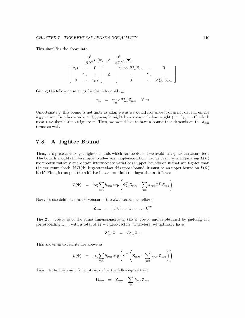
CHAPTER 7. THE REVERSE JENSEN INEQUALITY 146
This simplifies the above into:
∂2
∂Ψ2H(Ψ) ≥ ∂2
∂Ψ2L(Ψ) r1I · · · 0
.... . .
...0 · · · rMI
≥
maxnZT1nZ1n · · · 0
.... . .
...0 · · · ZT
MnZMn
Giving the following settings for the individual rm:
rm = maxnZT
mnZmn ∀ m
Unfortunately, this bound is not quite as adaptive as we would like since it does not depend on thehmn values. In other words, a Zmn sample might have extremely low weight (i.e. hmn → 0) whichmeans we should almost ignore it. Thus, we would like to have a bound that depends on the hmn
terms as well.
7.8 A Tighter Bound
Thus, it is preferable to get tighter bounds which can be done if we avoid this quick curvature test.The bounds should still be simple to allow easy implementation. Let us begin by manipulating L(Ψ)more conservatively and obtain intermediate variational upper bounds on it that are tighter thanthe curvature check. If H(Ψ) is greater than this upper bound, it must be an upper bound on L(Ψ)itself. First, let us pull the additive linear term into the logarithm as follows:
L(Ψ) = log∑mn
hmn exp
(ΨT
mZmn −∑mn
hmnΨTmZmn
)
Now, let use define a stacked version of the Zmn vectors as follows:
Zmn = [~0 ~0 . . . Zmn . . . ~0]T
The Zmn vector is of the same dimensionality as the Ψ vector and is obtained by padding thecorresponding Zmn with a total of M − 1 zero-vectors. Therefore, we naturally have:
ZTmnΨ = ZT
mnΨm
This allows us to rewrite the above as:
L(Ψ) = log∑mn
hmn exp
(ΨT
(Zmn −
∑mn
hmnZmn
))
Again, to further simplify notation, define the following vectors:
Umn = Zmn −∑mn
hmnZmn

CHAPTER 7. THE REVERSE JENSEN INEQUALITY 147
This lets us rewrite the L(Ψ) function compactly as:
L(Ψ) = log∑mn
hmn exp(ΨT Umn
)To compute our reverse-Jensen bound, we must set the scalars rm such that the inequality H(Ψ) ≥L(Ψ) holds for all values of Ψ. More specifically we need:
12
∑m
rmΨTmΨm ≥ log
∑mn
hmn exp(ΨT Umn
)∀Ψ
Selecting rm values such that the above holds for any Ψ vector requires considering all Ψ configu-rations in the whole multidimensional Euclidean space. For now, we shall simplify this multidimen-sional problem by only consider a one-dimensional ray in Ψ-space.
7.8.1 Bounding a One Dimensional Ray
However, for now, let us consider guaranteeing the bound when Ψ is along a certain given direction,i.e. Ψ. Therefore, we can write the Ψ vector as:
Ψ = βΨ
Thus, our L(Ψ) function becomes:
L(βΨ) = log∑mn
hmn exp(βΨT Umn
)Now, let us see if we can find a quadratic bound on the above uni-dimensional function alone. Inother words:
12qΨβ2 ≥ log
∑mn
hmn exp(βΨT Umn
)∀ β (7.5)
In the above, we have to find a scalar qΨ that satisfies the inequality for all β. The subscript onthe q indicates that it corresponds to a certain choice of direction Ψ. This will give us a quadraticbound along this directional slice. The hope is that these individual uni-dimensional bounds canbe aggregated and then used to find the required H(Ψ) in the full multi-dimensional problem. Forconvenience, define the scalars vmn as follows:
vmn = ΨT Umn
At this point, however, the problem has simplified to solving the following one-dimensional boundfor a value of qΨ:
12qΨβ2 ≥ log
∑mn
hmn exp (βvmn) (7.6)
It should be evident from the definitions of vmn (or more specifically the original definition of Umn)that the following holds: ∑
mn
hmnvmn = 0

CHAPTER 7. THE REVERSE JENSEN INEQUALITY 148
Consequently, when β is zero, both the left hand side above and the right hand side are zero andtheir derivatives are zero too (i.e. tangential contact). This one-dimensional log Gibbs partitionfunction is depicted in Figure 7.8 for various random configurations of the vmn and hmn as well asthe lower bounds that arise from the epigraph for visualization. These types of structures need tobe upper bounded by a quadratic.
−30 −20 −10 0 10 20 30−2
0
2
4
6
−30 −20 −10 0 10 20 30
−2
0
2
4
6
8
10
−30 −20 −10 0 10 20 30
−2
0
2
4
6
8
10
12
−30 −20 −10 0 10 20 30−2
0
2
4
6
8
−20 −10 0 10 20−10
0
10
20
30
Figure 7.8: One Dimensional Log Gibbs Partition Functions. The solid line is the Gibbs partitionfunction which is lower bounded by its epigraph (dashed red lines). These were plotted from l(β) =log∑
mn hmn exp(βvmn) for random selections of hmn and vmn.
For brevity, we will use l(β) to denote the right hand side of Equation 7.5.
l(β) = log∑mn
hmn exp (βvmn)
Instead of working directly with l(β), we will try to find an intermediate upper bound on thisquantity which has the following simpler form:
l(β) ≤ log (γ exp (βu) + γ exp (−βu) + 1− 2γ) (7.7)
This intermediate bound is interesting since it serves to symmetrize l(β) such that the sign of β isno longer important. This intermediate has two scalar parameters: u and γ. The right hand termabove is a variational bound which makes tangential contact with the left hand side at β = 0. Inother words, both sides are zero and have zero gradient at β = 0. We must now find legitimateparameters u and γ which will guarantee that the right hand side’s term is an upper bound. To doso, it suffices to find parameters which guarantee that the curvature of the right hand term is anupper bound on the curvature of the left hand term (since the 0th and 1st order terms are equalat β = 0). This is because of the flat tangential contact at β = 0. Thus, we need to guarantee thefollowing (this is the above Inequality 7.7 with the logarithm extracted out):∑
mn
hmn exp (βvmn) ≤ γ exp (βu) + γ exp (−βu) + 1− 2γ
Taking second derivatives with respect to β of both sides, we obtain the following (this is a strictercurvature test for the above inequality):∑
mn
hmnv2mn exp (βvmn) ≤ γ exp (βu) u2 + γ exp (−βu) u2 (7.8)
Let us now set the u parameter as follows: u = maxmn |vmn|. Now, instead of satisfying Equation 7.8we will satisfy the following two stricter constraints. These 2 cases subsume Equation 7.8 since ineach case we are subtracting a positive quantity from the left hand side and still trying to maintainan upper bound. These cases are as follows:

CHAPTER 7. THE REVERSE JENSEN INEQUALITY 149
• Case 1: When β is positive, we know that: exp(βu) ≥ exp(βvmn). This is because we alreadydefined u = maxmn |vmn| and β is positive. Thus we impose the following stricter guaranteeand expand it:
γ exp(βu)u2 ≥∑mn
hmnv2mn exp (βvmn)
γ exp(βu)u2 ≥∑mn
hmnv2mn exp (βu)
γ ≥∑
mn hmnv2mn
u2
• Case 2: When β is negative, we know that exp(−βu) ≥ exp(βvmn). Therefore, we impose thestricter guarantee below and expand it:
γ exp(−βu)u2 ≥∑mn
hmnv2mn exp (βvmn)
γ exp(−βu)u2 ≥∑mn
hmnv2mn exp (−βu)
γ ≥∑
mn hmnv2mn
u2
We can thus satisfy Inequality 7.7 by setting the following definition for the parameters γ and u andguarantee that the intermediate bound is valid. Thus, we have an intermediate upper bound on thelog Gibbs partition function which simplifies its possibly large number of terms (in the summation∑
mn) to just two parameters. Figure 7.9 depicts the bound for various random cases.
u := maxmn |vmn| γ :=∑
mnhmnv2
mn
u2
−30 −20 −10 0 10 20 30
0
0.5
1
1.5
−30 −20 −10 0 10 20 30
−2
0
2
4
6
8
10
−30 −20 −10 0 10 20 30
−10
0
10
20
30
40
50
60
−30 −20 −10 0 10 20 30
−2
0
2
4
6
8
10
−30 −20 −10 0 10 20 30
−2
0
2
4
6
8
10
12
Figure 7.9: Intermediate Bound on Log Gibbs Partition Functions. The solid line is the simpleintermediate upper bound which is always guaranteed greater than Gibbs partition function in thedashed red line.
Thus, instead of finding a qΨ that satisfies the original uni-dimensional bound in Equation 7.6 wewill merely find qΨ that satisfies the stricter intermediate bounds we have just computed:
12qΨβ2 ≥ log (γ exp (βu) + γ exp (−βu) + 1− 2γ) (7.9)
We next invoke a simple change of variables to get rid of the u parameter for the following analysis.Namely, define ω = βu and solve for the desired qΨ as follows:
qΨ
2u2≥ max
ωf(γ, ω)

CHAPTER 7. THE REVERSE JENSEN INEQUALITY 150
01
23
4
0
0.5
10
0.2
0.4
0.6
0.8
1
ωγ
f(γ,
ω)
Figure 7.10: f(γ, ω).
Where above we have replaced the expression on the right for brevity with a two-dimensional functionf(γ, ω). The 2d function is plotted in Figure 7.10 and is given by the following:
f(γ, ω) =log (γ exp(ω) + γ exp(−ω) + 1− 2γ)
ω2
0 0.2 0.4 0.6 0.8 10
0.1
0.2
0.3
0.4
0.5
0.6
0.7
0.8
0.9
1
γ
max
ω
f(γ,
ω)
Figure 7.11: maxω f(γ, ω).
Unfortunately, maximizing over ω cannot be done analytically. Instead, one possibility is to obtainthe function maxω f(γ, ω) numerically as show in Figure 7.11. Instead of dealing with maxω f(γ, ω)directly (which may be awkward due to its non-analytic nature), we can work with analytic linearupper bounds upon it. For example, we can have various linear upper bounds of the form:
aγ + b ≥ maxω
f(γ, ω)
0 0.2 0.4 0.6 0.8 10
0.2
0.4
0.6
0.8
1
γ
max
ω f(
γ,ω
)
Figure 7.12: Linear Upper Bounds on the numerical maxω f(γ, ω). Here, we show various settingsof the upper bounds aγ + b as we vary the (a, b) settings.
Figure 7.12 depicts the linear bounds on the maxω f(γ, ω) function. Some values of a and b whichprovide numerically guaranteed upper bounds on the right hand side are listed in the Appendix in

CHAPTER 7. THE REVERSE JENSEN INEQUALITY 151
Table 10.3. Matlab code to derive the function relating a and b is also given in the Appendix inSection 10.3. We merely have to select one of those many valid settings for a and b to obtain anupper bound on maxω f(γ, ω). Therefore, inserting this intermediate bound allows us to obtain thedesired qΨ in terms of the (a, b) linear bound:
qΨ ≥ 2u2 maxω
f(γ, ω)
qΨ ≥ 2u2(aγ + b)
qΨ ≥ 2 maxmn
v2mn
(a
∑mn hmnv2
mn
maxmn v2mn
+ b
)qΨ ≥ 2a
∑mn
hmnv2mn + 2b max
mnv2
mn
−30 −20 −10 0 10 20 30
−0.5
0
0.5
1
1.5
2
2.5
−30 −20 −10 0 10 20 30
−1
0
1
2
3
4
5
6
−30 −20 −10 0 10 20 30−2
0
2
4
6
8x 10⁻¹⁰
−30 −20 −10 0 10 20 30−0.02
0
0.02
0.04
0.06
0.08
−30 −20 −10 0 10 20 30
−1
0
1
2
3
4
5
6
Figure 7.13: Quadratic Bound on Log Gibbs Partition Functions. The quadratic bound (’x’ greenline) is above the the simple intermediate upper bound (the solid blue line) which is above the Gibbspartition function (dashed red line).
In the above, we have expanded our parameters u and γ in terms of their definitions. Figure 7.13depicts the desired resulting quadratic bounds from the formula for qΨ on the intermediate boundsas in Equation 7.9. We optimize over the possible choices (a, b) such that the qΨ value is minimizedto generate the tightest bound. We have thus found a quadratic bound for the one dimensional case.The next step is to fold this bound into the original multidimensional formulation and guarantee itin the general full-dimensional bounding problem.
7.8.2 Scaling Up to the Multidimensional Formulation
We now have a quadratic bound that is guaranteed along a particular slice of the L(Ψ) functionwhen Ψ = βΨ. Let us rewrite this unidimensional bound in terms of our whitened data vectorsZmn. Furthermore, for computational efficiency we will also make sure that the computation of qΨ
will only require simple inner products of these vectors. First recall the following definition:
vmn = ΨT
Zmn −∑ij
hijZij
Replacing that into the current bound on qΨ we get the following:
qΨ ≥ 2a∑mn
hmnv2mn + 2b max
mnv2
mn
qΨ ≥ 2a∑mn
hmn
ΨT
Zmn −∑ij
hijZij
2
+ 2b maxmn
ΨT
Zmn −∑ij
hijZij
2

CHAPTER 7. THE REVERSE JENSEN INEQUALITY 152
qΨ ≥ 2a∑mn
hmn
(ΨT Zmn
)2
− 2a
∑ij
hijΨT Zij
2
+ 2b maxmn
ΨT Zmn − ΨT∑ij
hijZij
2
For the terms that depend on the b scaling, we shall merely invoke Jensen’s inequality in a straight-forward way on the quadratic expression. Again, this makes us get an intermediate upper bound onqΨ which satisfies our requirements even more strictly. More specifically, we have:ΨT Zmn − ΨT
∑ij
hijZij
2
= 4×
12ΨT Zmn +
12
−ΨT∑ij
hijZij
2
≤ 4× 12
(ΨT Zmn
)2
+ 4× 12
ΨT∑ij
hijZij
2
Reinserting this bound into our current qΨ expressions, we obtain the following stricter conditionon qΨ:
qΨ ≥ 2a∑mn
hmn
(ΨT Zmn
)2
− 2a
∑ij
hijΨT Zij
2
+ 2b maxmn
2(ΨT Zmn
)2
+ 2
ΨT∑ij
hijZij
2
qΨ ≥ 2a∑mn
hmn
(ΨT Zmn
)2
− 2(a− 2b)
∑ij
hijΨT Zij
2
+ 4b maxmn
(ΨT Zmn
)2
We can easily guarantee that a − 2b is always positive (which is evident from the allowable valuesin the tables), and thus we see that the middle term in the above expression is negative. We cantherefore delete it and obtain an even stricter bound on qΨ:
qΨ ≥ 2a∑mn
hmn
(ΨT Zmn
)2
+ 4b maxmn
(ΨT Zmn
)2
Now recall the following property from the definition of Zmn in Equation 7.5. If we are dealingwith a normalized unit-norm version of the Ψ vector (i.e. Ψ), and dot product it with Zmn whichis padded with zeroes, this is equivalent to dot-producting the truncated version of Zmn with atruncated version of of Ψ, namely Ψm:
ΨT Zmn = ΨTmZmn
In the above we have the Ψm vector simply be a vector of less than unit norm corresponding to theunit norm vector Ψ with all entries that are not in the m’th index position zeroed out. This allowsus to rewrite the above as:
qΨ ≥ 2a∑mn
hmn
(ΨT
mZmn
)2
+ 4b maxmn
(ΨT
mZmn
)2
Any inner product can be written as the magnitudes of the vectors times the cosine of the anglebetween them, i.e. ΨT
mZmn = ‖Ψm‖ ‖Zmn‖ cos(θ). Therefore, we can find a stricter upper boundonce again by noting the following:(
ΨTmZmn
)2
≤ ΨTmΨmZT
mnZmn

CHAPTER 7. THE REVERSE JENSEN INEQUALITY 153
Therefore we can finally write the following condition on qΨ which will guarantee an upper bound:
qΨ := 2a∑mn
hmnΨTmΨm ZT
mnZmn + 4b maxmn
ΨTmΨm ZT
mnZmn
This definition of qΨ will give us a guaranteed quadratic bound on our original log-partition functionfor arbitrary choice of direction Ψ that:
12qΨβ2 ≥ log
∑m
∑n
hmn exp(βΨT Umn
)∀ β
We can now plug in the definition of qΨ in that quadratic expression and guarantee that it holds forany β and any Ψ:
12
(2a∑mn
hmnΨTmΨm ZT
mnZmn + 4b maxmn
ΨTmΨm ZT
mnZmn
)β2 ≥ log
∑m
∑n
hmn exp(βΨT Umn
)∀ β
We should point out here, that we can vary the chosen a and b values for each Ψ direction, theyneed not be fixed throughout to guarantee the bounds. In other words, they can be made functionsof the direction Ψ without violating the bound:(
aΨ
∑mn
hmnΨTmΨm ZT
mnZmn + 2bΨ maxmn
ΨTmΨm ZT
mnZmn
)β2 ≥ log
∑m
∑n
hmn exp(βΨT Umn
)∀ β
We now return to the original problem, which was finding a quadratic upper bound on a multi-dimensional log Gibbs partition function, i.e. H(Ψ) ≥ L(Ψ) by computing valid rm scalars thatsatisfy:
12
∑m
rmΨTmΨm ≥ log
∑m
∑n
hmn exp(ΨT Umn
)∀Ψ
The above can be written in terms of βΨ and then we can directly plug in the unidimensional boundwe have derived:12
∑m
rmβΨTmβΨm ≥ log
∑m
∑n
hmn exp(βΨT Umn
)∀ Ψ, β
12
∑m
rmβΨTmβΨm ≥
(aΨ
∑mn
hmnΨTmΨm ZT
mnZmn + 2bΨ maxmn
ΨTmΨm ZT
mnZmn
)β2 ∀ Ψ, β
We can now divide out the β2 (the β = 0 case is not relevant since we have tangential contact atβ = 0) from both sides:
12
∑m
rmΨTmΨm ≥
(aΨ
∑mn
hmnΨTmΨm ZT
mnZmn + 2bΨ maxmn
ΨTmΨm ZT
mnZmn
)∀ Ψ
By inspection, we can turn the above aggregate bound on the rm into M individual bounds onisolated rm. Satisfying these bounds on an individual basis will satisfy the aggregate bound:
12rmΨT
mΨm ≥ aΨ
∑n
hmnΨTmΨm ZT
mnZmn + 2bΨ maxn
ΨTmΨm ZT
mnZmn ∀ m

CHAPTER 7. THE REVERSE JENSEN INEQUALITY 154
Simplifying by dividing out the ΨTmΨm yields:
rm ≥ 2aΨ
∑n
hmnZTmnZmn + 4bΨ max
nZT
mnZmn ∀ m
Where we are still free to pick an arbitrary aΨ, bΨ pair for each m value. Thus, we should reallyindex those as:
rm ≥ 2am
∑n
hmnZTmnZmn + 4bm max
nZT
mnZmn ∀ m
The smallest value of rm which still satisfies the above is the tightest bound. Therefore, we set rm
to the above to obtain, finally, a succinct formula for it:
rm = 2am
∑n
hmnZTmnZmn + 4bm max
nZT
mnZmn ∀ m
Expanding out the definition wm − w′m = rm, we ultimately obtain:
wm = 2am
∑n
hmnZTmnZmn + 4bm max
nZT
mnZmn + w′m
Where we have (from previous sections) the following definition 2:
xsw′m = minw′m such thathm
w′m
(∂K(Θm)
∂Θm
∣∣∣∣Θm
−Xm
)+
∂K(Θm)∂Θm
∣∣∣∣Θm
∈ ∂K(Θm)∂Θm
And the Zmn are defined as follows (as shown earlier):
Zmn = K′′(Θm)−1/2(Xmn −K′(Θm))
It should be noted that we can always increase the wm terms and guarantee a bound because theseprovide a stricter bounding. Consequently, any of the intermediate terms in the computation of wm
which are too difficult to compute can be upper bounded if they result in an increase in the wm andthis will still guarantee a strict global bound.
7.9 Analytically Avoiding Lookup Tables
The use of lookup tables is mathematically unappealing so we instead now provide a fully analytictreatment of the am and bm tradeoff. Recall that we had achieved a fully analytic bounding processup until the point where we were trying to solve for qΨ:
qΨ
2u2≥ max
ω
log (γ exp(ω) + γ exp(−ω) + 1− 2γ)ω2
This bounding thus required the maximization over ω of the following function:
f(γ, ω) =log (γ exp(ω) + γ exp(−ω) + 1− 2γ)
ω2
2The value of w′m depends on the nature of the constraints on the Km function. In the Gaussian case, Θ is an
arbitrary Euclidean vector and therefore w′m is always zero. In the multinomial and other cases, it is trivial to compute
w′m with some simple algebra.

CHAPTER 7. THE REVERSE JENSEN INEQUALITY 155
It was deemed too difficult to exactly solve the max of f(γ, ω) and instead it was handled numerically.However, what we can do is find an upper bound on maxω f(γ, ω) and thus provide an even strictercondition on qΨ. Naturally, this bound will not be as tight as the one resulting from the a, b numericallinear bounds yet is fully analytic. First let us define the function g(γ) := maxω f(γ, ω) which wehave found too hard to compute analytically. We thus have:
qΨ = 2u2g(γ)
An analytic expression for g(γ) is too difficult, however note the following interesting property: 3:
g(γ) = γ ∀ γ ≥ 16
This is true, since the limit of f(γ, ω) as ω goes to zero (via l’Hopital’s rule) is:
limω→0
log(γ exp(ω) + γ exp(−ω) + 1− 2γ)ω2
= γ
The maximum of f(γ, ω) occurs at ω → 0 whenever γ ≥ 1/6. This is done by proving that:
log(γ exp(ω) + γ exp(−ω) + 1− 2γ)ω2
≤ γ
The proof of the last inequality is equivalent to proving:
exp(ω) + exp(−ω)− 2 ≤ exp(γω2)− 1γ
Expanding all exp functions into power series in ω and comparing terms yields the result. Thislast inequality can also be used to show that if 0 < γ < 1/6 then g(γ) > γ. Thus, we know thatg(γ) = γ for γ ≥ 1/6. Recall that g(γ) arose when we were trying to find a quadratic bound on thelog(γ exp(ω) + γ exp(−ω) + 1− 2γ). Thus, we had:
qΨ
2u2ω2 ≥ log(γ exp(ω) + γ exp(−ω) + 1− 2γ)
Evidently, then, if γ ≥ 1/6, we have:
qΨ ≥ 2u2γ ∀ γ ≥ 16
Now, let us look more closely at the interval when γ ≤ 1/6. For simplicity We define h(γ, ω) asfollows:
h(γ, ω) = log(γ exp(ω) + γ exp(−ω) + 1− 2γ)
Replacing, we can rewrite our condition as follows:
qΨ
2u2ω2 ≥ h(γ, ω)
3This property was noted and proved with the help of Dr. Michael Ulm, FB Mathematik, Universitaet Rostock.

CHAPTER 7. THE REVERSE JENSEN INEQUALITY 156
Let us now split the left hand side and the right hand side into two components:
q1
2u2ω2 +
q2
2u2ω2 ≥ h1(γ, ω) + h2(γ, ω) (7.10)
Naturally, we have:
qΨ = q1 + q2
h(γ, ω) = h1(γ, ω) + h2(γ, ω)
Now, if we can guarantee the following individual inequalities we can guarantee a stricter version ofthe overall inequality in Equation 7.10.
q1
2u2ω2 ≥ h1(γ, ω)
q2
2u2ω2 ≥ h2(γ, ω)
So far, he solution has not really developed any further through this breakdown. However, we willnext specify the h1 and h2, and we shall be able to find a simple analytic solution for q1 and q2.
For h1(γ, ω), we will use the following function:
h1(γ, ω) =|ω − log(γ)| − (ω − log(γ))
2+| − ω − log(γ)| − (−ω − log(γ))
2
The h2(γ, ω) is then naturally constrained to be:
h2(γ, ω) = h(γ, ω)− h1(γ, ω)
−10 −5 0 5 10−1
0
1
2
3
4
5
6
ω
h(γ,
ω)
−10 −5 0 5 10−1
0
1
2
3
4
5
6
ω
h 1(γ,ω
)
−10 −5 0 5 10−1
0
1
2
3
4
5
6
ω
h 2(γ,ω
)
(a) h(γ, ω) (b) h1(γ, ω) (c) h2(γ, ω)
Figure 7.14: Bounding Separate Components.
Clearly h1(γ, ω) and h2(γ, ω) add to form h(γ, ω) so this breakdown is legitimate. Figure 7.14 depictsthe different functions, h(γ, ω), h1(γ, ω) and h2(γ, ω). Now, it is relatively easy to upper bound theabove h1(γ, ω) and h2(γ, ω) functions individually. Basically, h1(γ, ω) is a symmetric function andwe can deal with only one side at a time. When ω ≥ 0, we need only guarantee that the quadraticbound is greater than a line with slope=1 and an ω-intercept of − log(γ). Therefore, we have:
q1
2u2ω2 ≥ ω + log(γ)
It is straightforward to show that:
14 log(1/γ)
ω2 ≥ ω + log(γ)

CHAPTER 7. THE REVERSE JENSEN INEQUALITY 157
This also holds for the ω ≤ 0 case by symmetry. Therefore, we obtain q1 as follows:
q1 =2u2
4 log(1/γ)
Now, we need to solve for q2 to upper bound h2(γ, ω). Again, by symmetry of h(γ, ω) and thequadratic upper bound, we need only consider the case when ω ≥ 0. We shall split the interval wherewe will verify this bound into two separate components: 0 ≤ ω ≤ log(1/γ) and log(1/γ) ≤ ω <∞.
For the first interval, log(1/γ) ≤ ω <∞, we see that h2(γ, ω) simplifies as follows:
q2
2u2ω2 ≥ h2(γ, ω) log(1/γ) ≤ ω <∞
q2
2u2ω2 ≥ h(γ, ω)− (ω − log(1/γ)) log(1/γ) ≤ ω <∞
Thus, we can find q2 by maximizing as follows:
q2
2u2= max
log(1/γ)≤ω<∞
h(γ, ω)− ω − log(γ)ω2
q2
2u2= max
log(1/γ)≤ω<∞
log(γ exp(ω) + γ exp(−ω) + 1− 2γ)− ω − log(γ)ω2
It is clear in the above that the numerator h(γ, ω) − ω − log(γ) is monotonically decreasing (itsgradient is always negative). Meanwhile, the denominator ω2 is monotonically increasing. Therefore,to maximize the fraction, we want to keep ω as small as possible, thus we set it to ω = log(1/γ).This gives us the following condition for q2:
q2
2u2=
log(γ exp(− log(γ)) + γ exp(log(γ)) + 1− 2γ) + log(γ)− log(γ)log(γ)2
(7.11)
q2
2u2=
log(γ2 − 2γ + 2)log(γ)2
(7.12)
For the second interval, 0 ≤ ω ≤ log(1/γ), and there h1(γ, ω) is simply zero. This permits h2(γ, ω)to simplify to: h2(γ, ω) = h(γ, ω). Therefore, we need to upper bound as follows:
q2
2u2ω2 ≥ h2(γ, ω) 0 ≤ ω ≤ log(1/γ)
q2
2u2ω2 ≥ h(γ, ω) 0 ≤ ω ≤ log(1/γ)
q2
2u2ω2 ≥ log(γ exp(ω) + γ exp(−ω) + 1− 2γ) 0 ≤ ω ≤ log(1/γ)
By concavity of the logarithm function, we can upper bound log(z) by z−1. If we invoke this upperbound on the right hand side, we obtain an even stricter condition for q2.
q2
2u2ω2 ≥ (γ exp(ω) + γ exp(−ω) + 1− 2γ)− 1 0 ≤ ω ≤ log(1/γ)
q2
2u2= γ max
0≤ω≤log(1/γ)
exp(ω) + exp(−ω)− 2ω2
The right hand side function being maximized over ω is monotonically increasing (its gradient isalways positive). Therefore, to maximize it, we set ω as large as possible within the interval being

CHAPTER 7. THE REVERSE JENSEN INEQUALITY 158
considered (i.e. ω = log(1/γ)). Thus, to satisfy the bounding for this interval, we obtain thefollowing condition on q2:
q2
2u2= γ
exp(− log(γ)) + exp(log(γ))− 2log(γ)2
(7.13)
q2
2u2=
(γ − 1)2
log(γ)2(7.14)
q2 = 2u2 (γ − 1)2
log(γ)2(7.15)
Now we must aggregate both Equation 7.12 with Equation 7.15 to obtain an overall bound on q2 forboth intervals. It is clear that Equation 7.15 is always stricter and subsumes Equation 7.12 sincethe following is provably true (by simply invoking the log(z) ≥ z − 1 rule):
(γ − 1)2 ≥ log(γ2 − 2γ + 2)
Therefore, we have the following values for q1 and q2 (when γ ≤ 1/6):
q1 =2u2
4 log(1/γ)
q2 = 2u2 (γ − 1)2
log(γ)2
Therefore, we can now compute the qΨ value as their sum:
qΨ = q1 + q2
qΨ = 2u2
(1
4 log(1/γ)+
(γ − 1)2
log(γ)2
)
This is only for the γ ≤ 1/6 region. We can combine it with our value for the γ ≥ 1/6 as follows:
qΨ = 2u2
{γ γ ≥ 1/6
14 log(1/γ) + (γ−1)2
log(γ)2 γ ≤ 1/6
For reasons that will become evident soon, the l0 discontinuity at γ = 1/6 is not desirable andprevents the overall concavity (with respect to the γ variable) of the right hand side. By checkingthe curvature of 1
4 log(1/γ) and (γ−1)2
log(γ)2 , we can see that these two functions are concave for γ ≤ 1/6.However, the sudden jump to the linear function when γ = 1/6 prevents concavity. To maintainconcavity, we use a linear upper bound for γ ≥ 1/6 which keeps the l0 and l1 continuity. Thus, wewill replace qΨ with a concavified version as follows:
qΨ = 2u2
{mγ + b γ ≥ 1/6
14 log(1/γ) + (γ−1)2
log(γ)2 γ ≤ 1/6
The gradient and the value at γ < 1/6 are:
m =1
4γ log(γ)2+
2(γ − 1)log(γ)2
− 2(γ − 1)2
γ log(γ)3
∣∣∣∣γ=1/6

CHAPTER 7. THE REVERSE JENSEN INEQUALITY 159
m =1
4/6 log(6)2+−5/3
log(6)2+
3(5/3)2
log(6)3
m ≈ 1.397
b =(
14 log(6)
+25/36log(6)2
)− m
6
In fact, to maintain concavity the value of m can be any value less than the slope computed above.However, we also must make it upper bound the original value, i.e. mγ + b ≤ γ for 1/6 ≤ γ ≤ 1.Therefore, we can merely use the value m = 1 (which would result in a b > 1/6 and thus an upperbound on the original linear γ function). Therefore, we obtain:
qΨ = 2u2
{γ + 1
4 log(6) + 25/36log(6)2 − 1/6 γ ≥ 1/6
14 log(1/γ) + (γ−1)2
log(γ)2 γ ≤ 1/6
In the next section we will justify why we went through the trouble to concavify the above functionover γ. Returning to our original solution for qΨ we had:
qΨ ≥ 2u2g(γ)
Therefore, we effectively have derived a guaranteed concave upper bound on g(γ). This analyticupper bound on g(γ) is depicted in Figure 7.15 and is given by the following equation.
g(γ) ≤
{γ + 1
4 log(6) + 25/36log(6)2 − 1/6 γ ≥ 1/6
14 log(1/γ) + (γ−1)2
log(γ)2 γ ≤ 1/6
0 0.2 0.4 0.6 0.8 10
0.2
0.4
0.6
0.8
1
1.2
1.4
γ
g(γ)
and
G(γ
)
0 0.02 0.04 0.06 0.08 0.10
0.05
0.1
0.15
0.2
0.25
0.3
γ
g(γ)
and
G(γ
)
Figure 7.15: Bounding the Numerical g(γ) (dashed red line) with Analytic G(γ) (solid blue line).
7.10 A Final Appeal to Convex Duality
We shall now explain why we have gone through this procedure to obtain an analytic concave upperbound on the g(γ) function. Let us define our new upper bound on the right hand side of the aboveexpression as G(γ), i.e. g(γ) ≤ G(γ). Figure 7.15 depicts the two functions. Also, we have alreadyshown that G(γ) is concave.
G(γ) =
{γ + 1
4 log(6) + 25/36log(6)2 − 1/6 γ ≥ 1/6
14 log(1/γ) + (γ−1)2
log(γ)2 γ ≤ 1/6

CHAPTER 7. THE REVERSE JENSEN INEQUALITY 160
Recall that we avoided working with g(γ) directly by only considering upper bounds on it of theform aγ + b ≥ g(γ). Ultimately, our final solution to the derived bounds had the form below whichinvolved these varying (a, b) terms:
wm = 2am
∑n
hmnZTmnZmn + 4bm max
nZT
mnZmn + w′m
The idea here is to now minimize the wm quantities above with respect to all possible settings ofthe (a, b) term pairs to obtain as tight a bound as possible. By varying the tangential contact pointγ of the linear (a, b) bounds we obtain a continuum of variational bound (a, b) pairs parameterizedby a variable, say t, i.e. (a(t), b(t)). Alternatively, we may merely parameterize b as a function of ato avoid the additional dummy variable, therefore, we have a continuum of pairs (a, b(a)). We cannow write the above more succinctly as:
wm = mina
2a∑
n
hmnZTmnZmn + 4b(a) max
nZT
mnZmn + w′m
Manipulating further, we obtain:
wm = 4maxnZT
mnZmn
(min
aa
∑n hmnZT
mnZmn
2 maxnZTmnZmn
+ b(a))
+ w′m
Now note that we had defined the a and b pairs to upper bound as follows:
aγ + b(a) ≥ g(γ)
If instead, we satisfy the following stricter condition (i.e. since G(γ) ≥ g(γ)), we have a validalternative choice of for (a, b) pairs:
aγ + b(a) ≥ G(γ)
Manipulating further, we note that following convex-duality form:
b(a) ≥ G(γ)− aγ
b(a) = maxγ
G(γ)− aγ
It is well known that for any concave function G(γ), b(a) becomes its (negated) convex dual by theabove procedure. This is because b(a) is formed by the epi-graph of linear bounds on top of theconcave G(γ) function. This property allows us to use the following standard convex-duality result(see the Appendix Section 10.2 for further clarification):
G(γ) = mina
b(a) + aγ (7.16)
Using the notation in the Appendix where we show the basic result relating a function f to its dualf∗ , we can clearly see that the above holds if we define f(γ) := G(γ) and f∗(a) := −b(a).
Now, recall that we had the following minimization problem to obtain wm:
wm = 4maxnZT
mnZmn
(min
aa
∑n hmnZT
mnZmn
2 maxnZTmnZmn
+ b(a))
+ w′m

CHAPTER 7. THE REVERSE JENSEN INEQUALITY 161
In the above, we have seen that the G() function arises from a similar minimization. We obtainexactly the epi-graph definition of G() in Equation 7.16 if we simply define the term multiplying ain the above equation as γ:
γ =∑
n hmnZTmnZmn
2 maxnZTmnZmn
We clearly see that the minimization over a can therefore be avoided giving us the following analyticresult for the reverse-Jensen bound:
wm = 4maxnZT
mnZmn G
(∑n hmnZT
mnZmn
2 maxnZTmnZmn
)+ w′m
Thus, to compute the upper bounds, we need to merely solve for the max and the expected normsof Zmn and then plug in their ratio into the G() function and so on.
This concludes the derivation.
2
Chapter 8
Imitative Learning
It is by imitation, far more than by precept, that we learn everything;
Edmund Burke, 1729-1797
We have discussed generative and discriminative learning and seen how the two can be theoreticallyfused into a powerful hybrid. We will now see these ideas come together in an applied sense asa combination of discriminative and generative tools will be used in an imitation system. Ourmotivation for imitative learning as a useful tool for learning interactive autonomous agents wasalready outlined in the introduction. This chapter will outline details of our implementation. Theimitative architecture we will propose here uses perception to learn passively from a human teacheras he interacts with his environment. It then utilizes its resulting models to synthesize an interactivecharacter that responds appropriately to perceived external stimulus.
To acquire data from the human teacher, we will use a generative perception model that automati-cally represents the human’s visual and acoustic activity as well as the external stimulus presented tohim. A generative model is appropriate so that we can provide a priori structure to the complicatedperceptual domain as well as be able to sample from this model to create virtual animations ofthe teacher. This generative representation then feeds training data to a discriminative predictionsystem that learns to forecast the human’s measurements in response to stimuli. A discriminativesystem here is favored to focus resources on the prediction task. We wish to optimize performance onour ability to specifically predict the output behavior of an agent given the stimulus of the externalworld.
In the next sections we begin by describing the architecture behind such an imitative system andbriefly relate it to the Action-Reaction Learning (ARL) platform. Various key issues and limitationsare brought up and motivate important generative and discriminative learning tools. Subsequently,we present the data collection method and hardware. A generative model is then described to modelthe perceptual domain and describes visual data as well as auditory data in the form of coefficientvectors. A discriminative (conditional) hidden Markov model using CEM is then used to learn toforecast a time series of such audio-visual coefficient vectors. Subsequently, we apply these tools toa large dataset of human interactions and generate a program that learns behavior. A qualitativeas well as quantitative evaluation of the imitation learning is then given. We complete the chapterwith a brief summary and open questions.
162
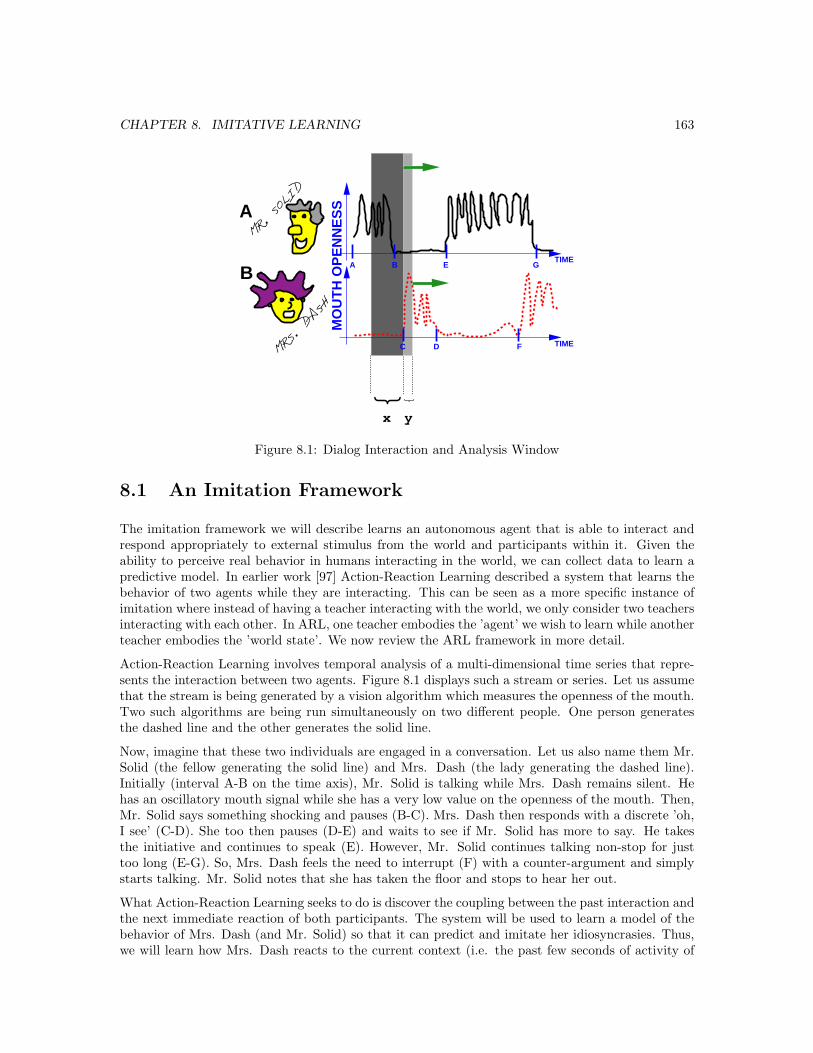
CHAPTER 8. IMITATIVE LEARNING 163
MR. SOLID
MRS. DA
SH
MO
UT
H O
PE
NN
ES
S
A B
C D
E
F
G
TIME
TIME
{ {x y
A
B
Figure 8.1: Dialog Interaction and Analysis Window
8.1 An Imitation Framework
The imitation framework we will describe learns an autonomous agent that is able to interact andrespond appropriately to external stimulus from the world and participants within it. Given theability to perceive real behavior in humans interacting in the world, we can collect data to learn apredictive model. In earlier work [97] Action-Reaction Learning described a system that learns thebehavior of two agents while they are interacting. This can be seen as a more specific instance ofimitation where instead of having a teacher interacting with the world, we only consider two teachersinteracting with each other. In ARL, one teacher embodies the ’agent’ we wish to learn while anotherteacher embodies the ’world state’. We now review the ARL framework in more detail.
Action-Reaction Learning involves temporal analysis of a multi-dimensional time series that repre-sents the interaction between two agents. Figure 8.1 displays such a stream or series. Let us assumethat the stream is being generated by a vision algorithm which measures the openness of the mouth.Two such algorithms are being run simultaneously on two different people. One person generatesthe dashed line and the other generates the solid line.
Now, imagine that these two individuals are engaged in a conversation. Let us also name them Mr.Solid (the fellow generating the solid line) and Mrs. Dash (the lady generating the dashed line).Initially (interval A-B on the time axis), Mr. Solid is talking while Mrs. Dash remains silent. Hehas an oscillatory mouth signal while she has a very low value on the openness of the mouth. Then,Mr. Solid says something shocking and pauses (B-C). Mrs. Dash then responds with a discrete ’oh,I see’ (C-D). She too then pauses (D-E) and waits to see if Mr. Solid has more to say. He takesthe initiative and continues to speak (E). However, Mr. Solid continues talking non-stop for justtoo long (E-G). So, Mrs. Dash feels the need to interrupt (F) with a counter-argument and simplystarts talking. Mr. Solid notes that she has taken the floor and stops to hear her out.
What Action-Reaction Learning seeks to do is discover the coupling between the past interaction andthe next immediate reaction of both participants. The system will be used to learn a model of thebehavior of Mrs. Dash (and Mr. Solid) so that it can predict and imitate her idiosyncrasies. Thus,we will learn how Mrs. Dash reacts to the current context (i.e. the past few seconds of activity of

CHAPTER 8. IMITATIVE LEARNING 164
the users which is akin to a world state). The process begins by sliding a window over the temporalinteraction as in Figure 8.1. The window looks at a small piece of the interaction and the immediatereaction of the users. This window over the time series forms the short term or iconic memory ofthe interaction and it is highlighted with a dark rectangular patch. The consequent reaction of Mrs.Dash and Mr. Solid are highlighted with the lighter and smaller rectangular strip. The first stripwill be treated as an input x and the second strip will be the subsequent future behavioral outputthey should generate (y). To predict and imitate what either Mrs. Dash or Mr. Solid will do next,a system system must estimate the future mouth parameters they will produce (these stored in y).As the windows slide across a training interaction between the humans, many such (x,y) pairs aregenerated and presented as training data to the system. The task of the learning algorithm is tolearn from these pairs and form a model relating x and y. Once learning has converged, it can thengenerate a predicted y∗ sequence whenever it observes a past x sequence. This allows it to computeand play out the future actions of one of the users (i.e. Mrs. Dash) when only the past interactionof the participants is visible.
Thus, the learning algorithm should discover some mouth openness behavioral properties. Forexample, Mrs. Dash usually remains quiet (closed mouth) while Mr. Solid is talking. However, afterSolid has talked and then stopped briefly, Mrs. Dash should respond with some oscillatory signal.In addition, if Mr. Solid has been talking continuously for a significant amount of time, it is morelikely that Mrs. Dash will interrupt assertively. A simple learning algorithm could be used to detectsimilar x data in another situation and then predict the appropriate y response that seems to agreewith the system’s past learning experiences.
Note now that we are dealing with a somewhat supervised learning system because the data has beensplit into input x and output y. The system is given a target goal: to predict y from x. However,this process is done automatically without any manual data engineering. One only specifies a-prioria constant width for the sliding window that forms x and the width of the window of y (usually,the width will be 1 frame for y to conservatively forecast only a small step into the future). Thesystem then operates in an unsupervised manner as it slides these windows across the data stream.Essentially, the learning uncovers a mapping between past and future to later generate its bestpossible prediction.
An interesting feature here (which we have stressed in the introduction chapter) is that the frameworkhas a shared action and perception space. Therefore, synthesizing an action that is similar toa perceived one would merely involve copying the corresponding parameters. We don’t need touncover or use some complicated mapping. The AIM (Active Intermodal Mapping) problem thatplagues many imitative learning approaches is effectively side-stepped. Therefore unraveling thecomplex mapping between a real human’s activity and a robot or virtual agent’s imitation of it isnot necessary.
8.1.1 A Simple Example
We now present a simple example of the ARL framework in action. This demonstrates the feasibilityof the approach in a particular domain but also permits us to later elucidate some weaknesses andmotivate important extensions.
Here, the agent learns to imitate a teacher’s head and hand gestures [97]. The world state is merelyanother person’s head and hand coordinates which the teacher is interacting with. Figure 8.2(a)depicts the training scenario where two users are interacting with each other by performing simplegestures while a camera tracks their head and hands coordinates. Tracking is done merely by

CHAPTER 8. IMITATIVE LEARNING 165
60 70 80 90 100 110 120−0.1
0
0.1
0.2
0.3
0.4
0.5
0.6
(a) (b)
Figure 8.2: A Gestural Imitation Learning Framework. In (a) two users are being tracked in real-time to collect measurements of their head and hand positions. Each user sees a caricature of theother in real-time on his screen. In (b), a time series of the perceptual measurements from one useris shown. Each step in time represents the means and covariances of the 3 Gaussians that describethe head and hand positions.
modeling skin-colored1 pixels in the image spatially as a mixture of three 2D Gaussians using EM.This gives us coordinates for the head and hands for both participants as a time series. Oneparticipant’s parameters (actually the mean and covariance of the skin-shaped Gaussians) are shownin Figure 8.2(b). At each time step of the training data, the users’ parameters over a window of thepast few seconds is vectorized. This large dimensional space is compressed with PCA down to 60dimensions and is used as input to predict the coordinates of the head/hands in the next frame (theoutput). The mapping from input to output is performed using a mixture of experts trained withmaximum conditional likelihood (CEM) over a few minutes of interaction.
Once we have learned from the training data, the model can be used to synthesize behavior inresponse to new stimuli. By feeding back the prediction and looping it with real measurements offof a human, the interactive agent responds to novel gestures in real-time. Figure 8.3 depicts theonline interaction process (after training) where a user is performing a tricky gesture and the virtualcharacter model claps in response to it. Several simple gestures and their appropriate context arethus learned from data and can be re-synthesized in a stochastic real-time manner when a singleuser gestures towards the system.
8.1.2 Limitations
We now discuss three important limitations of the ARL framework and lead into extensions and toolsthat will resolve them. First, the lack of a higher order mapping makes it hard to acquire long termbehavior. This is partly because we may not maintain the requisite fixed coordinate system of actionsand perceptions. The use of PCA as a representation also prevents us from inserting important priorknowledge and structure in our model of the perception and temporal activity and thus restrictsARL’s ability to generalize to novel behaviors. For example, simple yet nonlinear transformations ofthe training data may not be recognized by the model. Finally, ARL used conditional likelihood tofocus on predicting the future from the past which is not necessarily where the discrimination powershould be most appropriate. An alternative and more appropriate conditional criterion is predictingthe teacher’s actions (the one to be resynthesized) from another user’s actions which will always beobservable.
1The skin color distribution in RGB space itself is also modeled using EM and a mixture of 3D Gaussians.

CHAPTER 8. IMITATIVE LEARNING 166
Figure 8.3: Online Interaction with the Learned Synthetic Agent. The user is being tracked in real-time while the agent synthesizes the most likely reaction to his activity. The synthesis is a real-timeforecast and therefore varies according to slight variations in the human’s gestures.
CHAPTER 8. IMITATIVE LEARNING 167
Consistent and Long Term Training Data
As we previously mentioned, ARL avoids the AIM problem and has a direct equivalence betweenaction and perception. Thus we don’t have a layer of abstraction which will recognize that a givengesture remains the same from different perspectives and viewing conditions. Therefore, we musttake care that we maintain consistent representations and deal with changes in the coordinate systemup front (i.e. if the cameras are moved, etc.). This is because the action and perception layer arenot abstracted away for us by a higher order mapping. This often means that training data isshort and scarce because it must be constrained to have the same consistent view point. In thesetup above (Figure 8.2) we are relying on having a constant bird’s eye view of the scene and theparticipants. A real organism that performs imitative learning does not have the luxury of a fixedview point of its teacher. Organisms are often mobile and perform long term (or lifelong) learningin a multi-perspective world. Although we won’t show how to solve this problem explicitly, we willtry to alleviate it by proposing imitative ARL learning on a wearable platform that is affixed to andfollows a human teacher. This will let us extend the paradigm so that it can collect larger data setsfor training the behavior model.
A Generalizable Behavior Representation
To render the learning tractable, ARL projects the window over the short term memory into a 60dimensional approximation using PCA. This is reasonable since the time series data is made up ofsmooth trajectories. These will only get slightly smoothed from this approximation and will notlose too much detail (reconstruction accuracy is well above 90%). However, PCA may not be anappropriate representation since it does not capture any prior structure or knowledge we may haveabout the perceptual space or the temporal data. For example, a constant global translation of thehead and hands should not change the meaning of a gesture. Furthermore, speed and phase variationsin a gesture will also cause a radical change in a PCA representation even though the gesture itselfmay be the same. Unfortunately, these variations are not factored in the PCA representation anda subsequent predictive learning technique will have difficulty learning invariances to them andgeneralizing appropriately. Therefore, generative models are needed that can capture, or at leastrepresent in a factored way, these types of variations up-front (be they temporal warpings, visualtransformations or auditory variations).
Focusing on the Agent’s Output Behavior
Another deficiency in ARL framework is that it is discriminative in an inappropriate sense: it predictsthe future of both participants given the past. This regression model appropriately avoids wastingresources modeling the past when it has no predictive value for estimating the future (i.e. we optimizethe conditional p(future|past) and not the marginal p(past)). However, the past is not exactly givenwhen the system has to interact with a single human being in an online synthesis scenario. The onlydata that is ’given’ are the direct measurements from the external world and the single human whois triggering the system. Therefore, it would make more sense to try to form a conditional learningproblem where the conditioning of the variables is broken into p(agent|external world) where theexternal world may include other agents or other stimuli. While both measurements of the agent aswell as the world are available during training, during testing (or online prediction) only the externalstimulus will be available and it is up to the system to synthesize the agent’s output measurements.Therefore, this form of conditioning is more appropriate.

CHAPTER 8. IMITATIVE LEARNING 168
8.2 Long Term Behavior Data Collection
To resolve the issue of maintaining a consistent perception of the teacher’s behavior, we propose theuse of a wearable computer system. This is a convenient way to collect a sizeable amount of datawhile the teacher engages in various natural activities and also preserves the regular conditions andpoint of view necessary for a non-AIM based imitative learning framework. In Figure 8.4 a user(or teacher) has a head mounted microphone and a camera mounted to a boom that perceives hisface. This audio-video source is the perception space as well as the action space for the learner.Furthermore, a camera affixed to his glasses and a microphone that is aimed outwardly track thecontext (which is the perceived space for the external world). The wearable then collects data via asmall computer that transcribes both channels of audio-video signals at roughly 100 megabytes perhour.
Figure 8.4: Two channel audio-visual imitation learning platform.
Other instances of wearable learning include work by Starner [180] and Clarkson [38]. However,only the contextual space was modeled and the teacher’s action/perception data is not collected orcoupled to the external context as in the above system. The platform above provides a consistent wayto collect long-term data for the purposes of imitative learning without dealing with the problemsof mapping from action to perception.
8.2.1 Data and Processing
The video that is captured arrives at 7Hz in both cameras and is stored as images of size 60 by 80pixels in an 8-bit RGB representation. The images are first illumination-normalized by a histogramfitting operation. Then, the image is filtered using a Gaussian RGB mixture model of skin color toselect only the skin-colored pixels from the images in both video streams. This focuses modelingresources on the wearable user’s face and focuses the external stimuli on the head and hands ofpeople in the scene (as well as occasional random skin-colored objects, unfortunately).
The audio being captured arrives at a 16kHz sampling rate in mono for each microphone (with 16-bitresolution on amplitude). The audio is processed by computing its sound energy and thresholdingto avoid modeling insignificant background noise. Then we perform a fast Fourier transform over aHamming window (with 50% overlap) and use magnitude values of the audio only (the phase infor-mation is discarded). Each resulting spectrogram is clipped to use only the lowest 200 frequenciesof the audio signal (i.e. the highest represented frequency is about 6kHz). These spectrograms aregenerated at approximately 60Hz.
Figure 8.5 portrays several frames of the user as he walks down a hallway and approaches an

CHAPTER 8. IMITATIVE LEARNING 169
Figure 8.5: Wearable Interaction Data. Both the teacher and the world video are visible as well asthe spectrograms for their audio signals.

CHAPTER 8. IMITATIVE LEARNING 170
individual to begin conversation. The frames show both the user’s face and his own eye’s view(from the camera attached to his glasses). The spectrograms are shown interlaced between thecorresponding video images. The higher frequencies are to the left and more recent vectors are atthe bottom of each image. High intensities indicates high audio magnitude (the spectrograms arenormalized for easy viewing).
8.2.2 The Task
Given this large data set, our task will be to train an imitative agent by learning a good predictivemodel of what the teacher will do given the external stimulus. The data set which spans several hoursand hundreds of megabytes of images/spectrograms is initially split in half to form a training portionas well as a testing portion. Here, a piece of the training data is shown which covers approximately10 seconds worth of images (both the teacher and the external view) as well as 10 seconds worth ofspectrograms (from both microphones). The data is further split in half into a representation of theexternal world x (audio and video) and a representation of the agent y (audio and video). Therefore,we have x = world and y = agent. We now have a standard regression formulation where we needto obtain y from x by learning from the training data.
x
y
train test
Figure 8.6: The Audio-Visual Prediction Task. The user is seen conversing with another participantin the external video source. Both his video signal and the participant are shown over a few framesas well as their audio signals (as spectrograms). Using the training data portion, we wish to learna model that will map the outside world measurements x to the measurements y of the ’teacher’which the system will imitate.
8.3 Generative Modeling for Perception
As previous chapters argued, it would be naive to claim that the above raw sensory data we havecaptured (images and spectrograms) can be learned from directly without seeding the learningprocess with some structure. Although humans learn to see, learn to hear, and so forth, in a

CHAPTER 8. IMITATIVE LEARNING 171
machine learning system, this unwieldy learning task must be seeded with some a priori structures,models and algorithms to make it tractable. Without a priori structure, data requirements andsearch space size grow rapidly and lead to inefficient convergence. Such is the case for the blank-slate approaches to behavioral model learning that Edelman proposes in the Darwin series of robots(Darwin III, IV, V) [49]. Therein, the direct mapping of color responses from a camera into alarge unstructured neural network with connections to actuators does not seem practical and causesconvergence problems.
Of course, over-engineering the prior structure can be equally dangerous and there is a delicatebalance between nature and nurture. Not only can over-engineered structures specify models thatdon’t agree with the observed phenomena, providing too much extra knowledge and structure mightalso hurt. Extra knowledge and constraints can reduce tractability and computability. An algorithmwhich is guaranteed to find a global solution in polynomial time can be marred with local minimaand poor gradient descent solutions when unusual additional constraints (which capture additionaldomain knowledge) are added to the system. In Bayesian networks, the specification of dependenciesbetween random variable nodes is often restricted to a tree structure for propagation algorithms toconverge and additional knowledge may create non-trees or cyclic links [149] [209]. We will thuspropose a structured model that is not only intuitively plausible for the signals we will deal withbut is also algorithmically feasible.
In this section, we describe a structured generative model which we will to use to handle the variousperceptual signals being acquired by the hardware we proposed. We would like this model to quicklyprovide a useful and generalizable representation for the perceptual data that will be collectedfor imitation learning. Surprisingly, this generative model will be consistently applicable to boththe image data and auditory data we will be dealing with. Although it may seem naive initially,this generative model will permit a mapping of high-dimensional audio and video into a compactrepresentation which will greatly facilitate imitative learning.
Traditional ways to learn from and summarize complicated multi-variate data included, for example,principal components analysis (PCA)[20], factor analysis and multidimensional scaling [24]. Manysuch data summarization approaches can be cast in a generative model framework where latent valuesare estimated to compactly represent the data. Figure 8.8 depicts PCA as a generative Bayesiannetwork.
t=1..TC
X
V,Λ
t=1..TC
X1 X2 X3 XD
V,Λ
...
(a) (b)
Figure 8.7: A Bayesian Network Description of PCA. The model Θ includes eigenvectors and eigen-values V,Λ while the latent variables are the coefficients c. There are T instances of the data vector,X. The box acts as a replicator of the nodes T for all t = 1..T instances of the training data. Figure(a) depicts the data vectors as single nodes which is equivalent to (b) which merely zooms in oneach data vector by showing how it can be split into smaller tuples or its individual scalars 1..D.
Here, PCA’s model (i.e. Θ) is the eigenvectors and eigenvalues (V,Λ respectively). The data is theX node (which can be split into each dimension as sub-nodes X1, . . . , XD) while the coefficients c

CHAPTER 8. IMITATIVE LEARNING 172
can be thought of as latent variables. The nodes in the ’box’ drawing are replicated (T times forT instances of the data vectors). Given the eigenvectors, we are effectively forming a degenerateGaussian model that can be sampled to produce the data. The latent variables constrain thatGaussian to a single mean value which, when sampled, will generate a spherical Gaussian over thedata.
There are indeed many shortcomings with linear PCA as a representation which have encouragedvariants such as Bayesian PCA [21], independent components analysis [14], auto-associator networks[20], and nonlinear embedding [183]. However, in applying these techniques to images, audio andtime series, an important piece of knowledge is overlooked. All the aforementioned approachesassume the data they deal with can be rasterized directly into a vector form in a high-dimensionalEuclidean space.
However, images, audio, and time series are not vectors. A single color image is not a single bigvector but rather a collection of small vectors or tuples (pixels). Each of these tuples is vector of 5values, (X, Y,R, G,B) which specify XY location and RGB color. Similarly, an audio spectrogramis not a vector but rather a collection of 2-tuples (A,F ) where A is a band’s amplitude and F is itsfrequency. Furthermore, a univariate time series is not a vector, it is a collection of 2-tuples (C, T )or coefficient value C and time value T. This permits us to generate an interesting variant of PCAwhere each datum in our data set (images, audio) is not a vector but rather a collection of vectors.This modification of the model is depicted in Figure 8.8 as a Bayesian network.
t=1..TC
X1 X2 X3 XN
V,Λ
...
M1 M2 M3 MN...
Figure 8.8: Bayesian Network Representing a PCA Variant for Collections of Vectors.
Here, we have split each data vector X (image, audio data, time series) into the subcomponenttuples X1, . . . , XN which agree with our prior knowledge about the data’s structure. Since thereis no explicit ordering on a collection of pixels or tuples, we can no longer put them into somefixed vector arrangement. Instead, multinomial variables m1, . . . ,mN are introduced that assignan unknown discrete label to each subcomponent to associate it with a corresponding location oreigenvector subcomponent. Thus, the m1, . . . ,mN compute a correspondence between the data andthe model. Each mi multinomial parameter vector can be thought of as a vector of positive mixtureweights that sum to unity and effectively (in the hard case) picks a single destination assignment toan eigenvector component. We can stack the mi vectors to form a large M -matrix which can alsobe constrained to sum to unity across columns. These ’matching’ matrices are N × N and act assoft permutation matrices, re-sorting each data element’s tuples before we compute the eigenspace.In regular PCA, these M matrices are locked to identity. Instead, we will allow them to be variable,doubly-stochastic matrices. Unlike regular matching procedures which match only a pair of imagesor a pair of exemplars, the matching in this generative model is done simultaneously over the wholedata set. The M matrix elements can be appropriately repeated for each dimension in the tuple

CHAPTER 8. IMITATIVE LEARNING 173
(i.e. in an image that is XYRGB, our tuples our 5 elements creating a 5N × 5N matching matrix)to form a matrix that is the size of the x vector and we can image it transforming x as follows:
X = MX
This transform will re-shuffle the tuples, forming a new data element X such that the resultingeigenspace will fit more accurately and with less reconstruction error. It turns out that if we alsorestrict the summation over M ’s columns to be unity, we get a doubly stochastic matrix which forcesthe eigenvectors and the data tuples to distribute in a soft one-to-one manner. This is equivalentto a softened case of the so-called two-way assignment problem [17]. This problem has an exactpolynomial time solution called the Auction Algorithm [17]. However a statistical physics basedapproximation called the Invisible Hand Algorithm actually produces a more rapid result [112] 2.Although a standard EM-propagation framework to the above problem could be feasible, we favoredthis alternative solution because of the doubly stochastic constraints and the faster convergenceperformance. The computation effectively iterates PCA computations interlaced with the invisiblehand algorithm solutions until convergence (after a few dozen iterations). We compute the softassignment matrices, then the coefficients, then the eigenspace iteratively, one at a time, while theother parameters are fixed. The solution seems to converge yet does so non-monotonically and isplagued by local minima. Finding a cleaner more global model and algorithm would be interestingavenues for future research. We now explicate how to apply this generative model to images andaudio to finally form a multivariate time series of data.
8.3.1 A Generative Model on Images
We begin by collecting a small high-quality subset of images (a few hundred) of the agent and theexternal world after they have been skin-segmented (to obtain the faces). This data is then used toform a collection of (X, Y, I) tuples where I is the gray-scale intensity. Effectively, this representationtreats the images and pixels as “point-clouds” where a collection of 3D points is considered insteadof a continuous 2D intensity map. Approximately 2000 (X, Y, I) points are sampled from eachimage forming a speckled point-cloud representation of it. For each of these image sets in our data(agent and world), we then learn the latent coefficients, the doubly stochastic matrices as well asthe eigenspace using the structured PCA model in Figure 8.8.
Figure 8.9: Reconstruction of Facial Images with PCA and Variant.
Figure 8.9 depicts the model’s ability to reconstruct facial images of the teacher (after skin-colorbased segmentation) from a 20 dimensional representation (compare it with the reconstruction of
2As an interesting related side note, these same authors have also recently derived a statistical physics formulationfor handling loopy Bayesian Networks.

CHAPTER 8. IMITATIVE LEARNING 174
PCA directly on these images). The advantage of the collection of vectors is that morphing in XYis just as easy as varying RGB quantities.
The reconstruction error for the variant is up to 2.5 orders of magnitude better than PCA for thesame level of dimensionality reduction. Previous techniques in the literature also utilized opticalflow [18] or variations [143] of it for image matching and also produce better reconstruction thanPCA.
0 10 20 30 40 50 600
2
4
6
8
10
12x 10
5
Iterations
Squ
ared
Err
or
User Image Reconstruction
0 50 100 150 2000
1
2
3
4
5
6
7
8
9x 10
5
Iterations
Squ
ared
Err
or
World Image Reconstruction
(a) Agent Images (b) World Images
Figure 8.10: Reconstruction error for images of self (left) and world (right). 20 eigenvectors areused. The dashed red line depicts the reconstruction error of PCA while the solid blue line depictsthe variant.
In Figure 8.10 we show the reconstruction accuracy of the variant compared to PCA where bothuse a projection down to 20 eigenvectors. The variant captures much more of the image structureby permitting pixel permutation. The whole data set is then processed with the agent’s eigenspacewhere each agent image gets its own coefficients and matrix M . Each image is then summarizedby the 20-dimensional coefficient vector that results. Similarly, all the world images are processedforming 20-dimensional coefficient vectors for each.
8.3.2 A Generative Model on Spectrograms
Similarly, we can apply the variant to spectrograms since these are not vectors either. In fact aspectrogram has structure since it is several 2-tuples of amplitude and frequency. These can bepermuted to increase reconstruction accuracy over PCA as shown in Figure 8.11. Again, for 20eigenvectors, reconstruction accuracy is over 2 orders of magnitude better for the variant. Notethat we also factored out the magnitude (loudness) of the spectrogram from this representation andconcatenate it to the coefficient vector. This produces a 21-dimensional vector that summarizes the(200-dimensional) spectrogram data.
Spectrogram eigenspaces were learned for the agent’s audio and for the world’s audio from a smallsubset. Then, we compute the coefficient vectors for the whole data set of agent audio and worldaudio with their respective eigenspace to get a 21-dimensional coefficient vector for spectrogram ateach time point in the sequential dataset.

CHAPTER 8. IMITATIVE LEARNING 175
0 10 20 30 40 500
50
100
150
200
250
300
350
Iterations
Squ
ared
Err
or
User Spectrogram Reconstruction
0 50 100 1500
0.5
1
1.5
2
2.5x 10
5
Iterations
Squ
ared
Err
or
World Spectrogram Reconstruction
Figure 8.11: Reconstruction error for spectrograms of self (left) and world (right). 20 eigenvectorsare used. The dashed red line depicts the reconstruction error of PCA while the solid blue linedepicts the variant.
8.4 Hidden Markov Models for Temporal Signals
The above representations generate a 20 or 21 dimensional vector for each frame of agent audio, agentvideo, world audio and world video. By processing the whole data set, we obtain four multidimen-sional time series of these coefficients. These are then time-aligned (with appropriate interpolation)and aggregated into a large 82-dimensional time series. Unlike the previous ARL formulation wherePCA is used to represent a window over this time series, we shall instead describe the time serieswith a hidden Markov model. PCA does not have temporal invariance properties and thereforesuffers from temporal misalignments in the data. It is well known that a hidden Markov model iswell-suited to time series data and can effectively model time warpings and sequential variations.This arises by considering a hidden state variable and permitting summations of all possible statepaths in the evaluation of the probability of a sequence. Figure 6.1 depicts the graphical model fora hidden Markov model however we shall make some simple modifications such that it more directlyaddresses the desired task at hand.
8.5 Conditional Hidden Markov Models for Imitation
Since we are interested in predicting the component of the time series (audio and video) that theagent would generate, we now have a discriminative prediction task, namely to predict y. This couldbe cast in the MED framework by learning a regression function derived from HMM likelihoodmeasurements that would estimate the output with an epsilon-sensitive model. There are importantproblems with such an approach. Unlike a traditional regression setting, the output of the HMMmodel may exhibit some time-warpings and may not be perfectly aligned with the desired outputeven though it generates the appropriate behavior. Therefore, an epsilon-tube type of constraintmay be inappropriate since it forces the outputs to be perfectly matched in time on a sample-by-sample basis. Furthermore, performing MED regression requires the resolution of many two-sidedconstraints on the output scalars. Since the training data has hundreds of thousands of samplesas well as 20 output dimensions, the number of Lagrange multipliers would be in the millionsmaking training very cumbersome. Therefore we will employ a maximum conditional likelihood asour surrogate discriminative framework to estimate the input-output HMM instead [16]. We willbe discriminative in the conditional sense and utilize the CEM algorithm to estimate the HMM’sparameters as elaborated (with Jensen and reverse-Jensen inequality derivations) in Chapter 6.
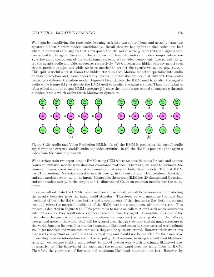
CHAPTER 8. IMITATIVE LEARNING 176
We begin by simplifying the time series learning task into two subproblems and actually learn twoseparate hidden Markov models conditionally. Recall that we had split the time series into halfwhere x represents the signals that correspond the the world while y represents the signals thatcorrespond to the agent. We can further split each of these into audio and video components wherexa is the audio component of the world signal while xv is the video component. The ya and the yv
are the agent’s audio and video sequences respectively. We will learn one hidden Markov model suchthat it predicts p(ya|xa, xv) while we learn another to predict the agent’s video, i.e. p(yv|xa, xv).This split is useful since it allows the hidden states in each Markov model to specialize into audioor video prediction and, more importantly, events in either domain occur at different time scalesrequiring a different transition model. Figure 8.12(a) depicts the HMM used to predict the agent’saudio while Figure 8.12(b) depicts the HMM used to predict the agent’s video. These form what isoften called an input-output HMM structure [16] since the inputs x are related to outputs y througha hidden state s which evolves with Markovian dynamics.
S1 S2 S3 S4 S5
Ya1 Ya2 Ya3 Ya4 Ya5
Xa1 Xa2 Xa3 Xa4 Xa5Xv1 Xv2 Xv3 Xv4 Xv5
S1 S2 S3 S4 S5
Yv1 Yv2 Yv3 Yv4 Yv5
Xa1 Xa2 Xa3 Xa4 Xa5Xv1 Xv2 Xv3 Xv4 Xv5
(a) (b)
Figure 8.12: Audio and Video Prediction HMMs. In (a) the HMM is predicting the agent’s audiosignal from the external world’s audio and video stimulus. In (b) the HMM is predicting the agent’svideo from the same input again.
We therefore train two input-output HMMs using CEM where we have 30 states for each and assumeGaussian emission models with diagonal covariance matrices. Therefore, we need to estimate theGaussian means, covariances and state transition matrices for both these models. The first HMMhas 21-dimensional Gaussian-emission models over ya in the output and 41-dimensional Gaussian-emission models over xa, xv in the input. Meanwhile, the second HMM has 20-dimensional Gaussian-emission models over yv in the output and 41-dimensional Gaussian-emission models over the xa, xv
input.
Since we will estimate the HMMs using conditional likelihood, we will focus resources on predictingthe agent’s behavior from the input world stimulus. Therefore, we will maximize the joint log-likelihood of both the HMM over both x and y components of the time series (i.e. both inputs andoutputs) minus the marginal likelihood of the HMM over the x component of the time series. Thisprocess is depicted in Figure 8.13. This permits us to focus on salient stimuli such as conversationswith others since they results in a significant reaction from the agent. Meanwhile, episodes of thedata where the agent is not expressing any interesting responses (i.e. walking alone in the hallway,background noise in the world, etc.) will be ignored even though they may contain much structure inthe world-signal on its own. In a standard maximum likelihood scenario, these external world stimuliwould get modeled and waste resources since they can be quite structured. However, their structuresmay not be important or useful in a task-related way and should not be modeled for their own sakeunless they provide information about the output y. Furthermore, in using a conditional likelihoodcriterion, we become slightly more robust to model inaccuracies which maximum likelihood maybe sensitive to. The behavior of the agent and the external world does not truly follow an HMM.Therefore, the guarantees of Bayesian and maximum likelihood estimation are lost. However, by

CHAPTER 8. IMITATIVE LEARNING 177
imposing the task (agent prediction) on the system via conditional maximum likelihood, we can beless sensitive to some aspects of model-data mismatch.
S1 S2 S3 S4 S5
Y1 Y2 Y3 Y4 Y5
X1 X2 X3 X4 X5
S1 S2 S3 S4 S5
X1 X2 X3 X4 X5
log p(x, y) − log p(x)
Figure 8.13: Conditional HMM Estimation. Effectively, we maximize the joint p(x, y) log-likelihoodof the HMM over both x and y (inputs and outputs) minus the marginal p(x) log-likelihood wherethe HMM has been summed over to obtain a marginal only over the x input.
The above optimization therefore requires us to maximize the conditional log-likelihood of the HMMparameters with respect to the time series of xt, yt vectors. This conditional log likelihood is simplylog p(x, y)−log p(x) yet these are latent distributions due to the state paths being hidden in an HMM.Therefore, we can write the conditional log-likelihood as: log
∑s p(s, x, y)− log
∑s p(s, x) where we
recognize the intractable log-sum and a negated log-sum forms as discussed in previous chapters.We utilize the Jensen inequality to lower bound the first term and the reverse-Jensen inequality tolower bound the second term. This then permits us to do a simple m-step to reestimate the HMM’sparameters. This process is therefore the CEM loop for HMMs and is iterated until convergence ofconditional likelihood.
8.6 Experiments
The hidden Markov models are trained as in Chapter 6. The audio prediction HMM is first initializedwith 5 iterations of EM and then converges with CEM to a maximum of conditional likelihood. Thevideo prediction HMM is optimized only with CEM after a random initialization. Due to the largesize of the dataset (the number of samples in the trellis is of the order of hundreds of thousands ofsamples), we could not compute the wm parameters exactly for the reverse-Jensen inequality andinstead used heuristics (described in Chapter 6) to make the optimization more efficient. Therefore,the monotonic convergence properties of CEM are compromised with these heuristics.
8.6.1 Training and Testing Likelihoods
The data set we have thus compiled is basically a 130,000 sample time series of multidimensionalvectors (82-dimensional to be precise). We use the first 75000 samples for training while the last55000 samples are used for testing. These each form one long continuous sequence and therefore, totrain the HMMs, we have to deal with trellis sizes of up to 75000 samples. The forward-backwardalgorithm and its counter-part for the reverse-Jensen inequality need special consideration to operateon such a lengthy trellis window. We begin by scaling the α, β probabilities in the forward-backwardalgorithm appropriately to avoid numerical errors [156]. Furthermore, we avoid computing thereverse-Jensen bounds exactly since their computation scales poorly with large trellis sizes (in terms

CHAPTER 8. IMITATIVE LEARNING 178
of number of samples and number of hidden states). Instead, we use the heuristic that wm = wm
where the reverse-Jensen bound’s width parameter is copied from the width parameter of the regularJensen bound (based on a symmetry type of argument).
Figure 8.14 depicts the convergence of the EM and the approximate CEM algorithm for the audio-prediction HMM. While EM converges monotonically to the maximum likelihood solution, it isinappropriate to optimize maximum likelihood in this setting since the world state (the x vectors)will always be measurable and need not be predicted or modeled on their own. Since we desire aconditional mapping from x to y, the conditional criterion is more suitable. Convergence for bothalgorithms required less than 30 minutes on a modest Pentium III machine.
0 10 20 30 40 50200
200.5
201
201.5
202
202.5
203
203.5
204
204.5
205
Iterations
Log−
Like
lihoo
d
Joint Log−Likelihood for Audio Predictor
0 10 20 30 40 50 6097
98
99
100
101
102
103
Iterations
Log−
Like
lihoo
d
Conditional Log−Likelihood for Audio Predictor
(a) (b)
Figure 8.14: Training Log-Likelihoods for Audio Prediction HMM. In (a) we show the joint log-likelihood per iteration and in (b) we show the conditional log-likelihood per iteration. The dashedred line is EM’s resulting log-likelihoods while the continuous blue line is CEM’s resulting log-likelihoods. Note the common starting point and the common first 5 EM-iterations for both algo-rithms. The use of heuristics to speed up the reverse-Jensen inequality for the HMM (trellis sizehere is T=75000) prevents monotonic convergence in CEM.
Figure 8.15 depicts a similar behavior of the learning algorithms on the video prediction HMM.Here the EM algorithm increases log-likelihood yet compromises conditional log-likelihood. TheCEM counterpart focuses resources in the opposite direction. Training time for both algorithmsrequired less than 30 minutes on a modest Pentium III machine.
The optimization of a surrogate conditional likelihood instead of ML is performed (i.e. CEM insteadof EM) since we ultimately would like to optimize conditional likelihood on the test data. To evaluatethe performance of our HMMs, we need to see how well they can estimate y from x. Therefore, it isunfair to evaluate performance on the test data with maximum likelihood. The x are always ’given’and therefore should not improve our score simply because we were able to predict them. Therefore,a predictive HMM that needs to generate y from x should be evaluated by a discriminative finalcriterion. However, unlike traditional classification problems where, for instance, classifier accuracyis a good performance metric, regression accuracy is not directly applicable to HMM forecasts andoutputs. Regression accuracy is a natural and acceptable performance metric in a static functionapproximation problem. However, the HMM’s outputs (just like its inputs) are sequences. Thesesequences can easily accommodate time-warping. Therefore, the HMM can generate time sequenceswith flexible time-warpings as well. It makes it inappropriate, consequently, to merely ’subtract’ anHMM’s regressed estimate from the testing data since the two may not be perfectly aligned. Forexample, consider the case where the output of our HMM was a sinusoid and it correctly matchedthe overall shape of the desired sinusoid in the testing output data. However, if a small phase shiftwere to arise, these two sinusoids would be misaligned and give rise to a large RMS error. It is unfairto penalize the HMM since it produced the desired overall behavior but was not in perfect alignment

CHAPTER 8. IMITATIVE LEARNING 179
0 10 20 30 40 50 60 70−10
−9
−8
−7
−6
−5
−4
Iterations
Log−
Like
lihoo
d
Joint Log−Likelihood for Video Predictor
0 20 40 60 80 100 120−110
−109.5
−109
−108.5
−108
−107.5
−107
−106.5
−106
−105.5
−105
Iterations
Log−
Like
lihoo
d
Conditional Log−Likelihood for Video Predictor
(a) (b)
Figure 8.15: Training Log-Likelihoods for Video Prediction HMM. In (a) we show the joint log-likelihood per iteration and in (b) we show the conditional log-likelihood per iteration. The dashedred line is EM’s resulting log-likelihoods while the continuous blue line is CEM’s resulting log-likelihoods. Note the common (random) starting point for both algorithms. The use of heuristics tospeed up the reverse-Jensen inequality for the HMM (trellis size here is T=75000) prevents monotonicconvergence in CEM.
with the testing data. Thus, it is often inappropriate to use static regression evaluation techniquesin an HMM setting. Instead, we will only report conditional likelihood accuracy on testing sinceother metrics do not capture the invariance in the predictions we would like to impose.
Log-Likelihood EM CEMJoint under Training 204.12 203.33Joint under Testing 202.55 202.22Conditional under Training 100.61 101.50Conditional under Testing 99.61 100.58
Table 8.1: Testing Log-Likelihoods for Audio Prediction HMM.
Table 8.6.1 depicts the testing log-likelihoods for the HMM on the agent’s audio prediction task. Wealso show the training likelihoods for comparison. Both EM and CEM perform as expected, yieldinggood joint likelihood and conditional likelihood test scores respectively. However, CEM performsbetter during conditional likelihood testing (matching the performance EM had during its training,in fact) which is the desired outcome. Note, here, that the reported quantities are on a logarithmicscale and therefore, in terms of likelihood, the CEM solution is at least 2.5 times more likely.
Log-Likelihood EM CEMJoint under Training -4.45 -4.96Joint under Testing -21.12 -20.61Conditional under Training -106.06 -105.73Conditional under Testing -122.46 -121.26
Table 8.2: Testing Log-Likelihoods for Video Prediction HMM.
The situation is a little more unusual in the video prediction task shown in Table 8.6.1. Here, thetesting log-likelihoods for the HMMs (and the training ones for that matter) are somewhat similarfor both EM and CEM. Part of the problem could be that the video signals have a slower time

CHAPTER 8. IMITATIVE LEARNING 180
scale than the audio ones so conditional learning may have less of a role. Furthermore, CEM’sconvergence was particularly poor here due to the speedup heuristics we are employing. CEM stillperforms better in terms of training and testing conditional likelihoods and, quite surprisingly, doesslightly better on testing under joint likelihood as well.
While the above results provide a quantitative evaluation of the models, algorithms and the datafit, it is not clear that the HMM prediction systems are capable of synthesizing imitative behaviorthat qualitatively matches our expectations. In the next section we show the results of using thepredictions to animate a synthetic character that mimics the agent teacher and comment anecdotallyabout the resulting behavior/performance.
8.7 Resynthesis Results
Given a generative model on the temporal data (i.e. the HMMs) as well as a generative model of theperceptual input (the structured variant of PCA), we can now synthesize agent reactions to test datawhere only the world stimulus is measured. This is done by first solving for the state distributions (i.e.trellis) using the measurements from the external stimuli alone. In other words, we use a marginalizedhidden Markov model where the Gaussian emission models are only over the x component of thetime series. The forward-backward algorithm then computes a distribution the hidden states in theHMM. Given the hidden states, it is straightforward to compute the expected value of the outputvectors yt at each time point by averaging the means of the Gaussian emissions weighted by theircorresponding state assignment probability. This method is reminiscent of other HMM regressionapproaches where we map an input variable to an output by first solving for the hidden states. Theseinclude matching visemes and phonemes [27], adding stylistic variations to dynamics [28], couplingmusical instrument expression to sound generation [173] as well as synthesizing facial expressionsbetween interacting people [73]. However, the HMMs we have estimated used CEM and thereforetheir parameters where optimized specifically for this type of task. More formally, we have thefollowing type of resynthesis (or regression):
yt =M∑
m=1
αt(m)βt(m)~µy(m)
The above α, β values are the standard (normalized) forward-backward probabilities while the µy(m)is the ’y’ vector component of the mean of the m’th Gaussian emission model (where m = 1..Mindexes the states of the HMM).
The hidden Markov models thus provide us with a time series of predicted vectors of audio andvideo coefficients for the agent. In other words, we have ya and yv for each time point. Given thesecoefficients, we can reconstruct the original signals (images and spectrograms) by simply multiplyingthe coefficients with the eigenvectors computed by the PCA variant. After some straightforwardoperations, it is possible to synthesize spectrograms and point-clouds. Unfortunately, the point-clouds are difficult to visualize and therefore, we merely find the closest nearest-neighbor in thetraining data to the vector yv and render the corresponding image of the agent at that time point.
8.7.1 Resynthesis on Training Data
We now describe the predictions that the HMMs produce when applied to the training data. Here,we censor the true outputs y and only show the input signal x, namely the external world measure-ments. We begin by double-checking the HMM’s performance on the training dataset. Since the

CHAPTER 8. IMITATIVE LEARNING 181
HMMs were trained on these exemplars, this process does not test their ability to generalize andsynthesize proper output behavior. Effectively, we are only evaluating the HMMs’ ability to encodethe training data and to repeat/mimic the behavior without extrapolation. What we can show is acompression argument since the HMM parameters effectively summarize the agent’s y signals muchmore compactly than the original training data representation. Each of the hidden Markov modelshas roughly 302 parameters for the transition matrix and 30×60 parameters for the Gaussian meanand Gaussian (diagonal covariance) parameters. Therefore, with a total of 9000 scalar parameters,we are trying to summarize a 41-dimensional time series with approximately 75,000 samples. Thus,3 million scalars are being captured using 9000 scalars. We obtain a compression level of over 3orders of magnitude when we encode the data with the HMMs. In principle, though, this is a roughestimate since the accuracy or number of significant digits of the scalars (in the data and in theHMM) has not been accurately specified.
We next show the resynthesis for a few thousand samples as in Figure 8.16 which spans samplevalues 1733 to 3209 (the training data spans time indices 0-74999 while the testing spans 75000-130000). This figure was generated by taking individual frames from real-time (5Hz) movies wegenerated from the HMM predictions and the reconstructed audio and video coefficients (the moviesare obviously easier to interpret than these figures yet unfortunately cannot be integrated into adocument). In the figure, we portray, from left to right order, the world audio spectrograms, theagent’s audio spectrograms, the ’cloud of points’ PCA representation of the external world faces, therepresentation of the agent’s face, then the raw video of the external world as well as the raw videoof the agent. The raw video of the agent is computed from the point-cloud’s representation from thePCA variant. We use the coefficient vector representing the cloud-point and find its nearest neighbor.This nearest neighbor match is found from all images in the training data set and their corresponding20-dimensional vector representations. Efficient nearest neighbor searching is implementing usingKD-trees. This lets us render the image that looks most like the point-cloud the generative modelis recovering. It was crucial to find a nearest neighbor raw video match since the cloud of pointsis a confusing representation and causes excessive speckling. Note, also, that the point clouds havebeen translated and centered to the middle of the image.
The spectrograms in Figure 8.16 are also shown. Here, time for the spectrograms increases as wemove from top to bottom in each image. Furthermore, as we move across the figure from image toimage, time increases from top to bottom of the figure. Spectrograms can be inverted to play backsound however there are synthesis problems since the phase information is no longer present (weonly model magnitudes). Although heuristics exist for reconstructing phase [75], we simplified theproblem by using random phase values. This causes a significant amount of noise and clicking inthe audio resynthesis but the audio is still discernible.
Observing Figure 8.16, we see the synthetic agent initiating a conversation as he approaches anindividual in the external world. The agent says “Hi” followed by the human saying “Hi”. Thenthe agent says “how are you” which the human replies “fine and you”. Most of the other agentarticulations are mumbles that are difficult to decipher and generally sound like “I see”, “hmm” and“yeah” except these are interleaved appropriately into the real human speech in the external worldstream. The agent also says what sounds like “hi” and “how are you” at semantically inappropriateplaces in the conversation yet are interleaved appropriately in terms of timing with the real human’sspeech and audio energy. Furthermore, there is some head movement and visual cues of speech inthe agent’s synthesized video during the times when the agent is generating audio.
In Figure 8.17, we skip a few seconds and go to the end of the conversation the agent is having withthis human and transition to the next person (time stamps 6265 to 7773). This is still data in thetraining set yet it is important to note that the agent maintains a similar interactive behavior eventhough there are many changes in audio/video signals as it transitions from one human to another.

CHAPTER 8. IMITATIVE LEARNING 182
1733)
1953)
2147)
2335)
2525)
2707)
2885)
3073)
3209)
Figure 8.16: HMM Resynthesis on Training Data. Time is increasing from top to bottom at about3 seconds per row. The figures are arranged from left to right as follows: the world spectrograms,the agent’s spectrograms, the centered world visual point-cloud, the agent’s visual point-cloud, theworld’s image data and the agent’s image data reconstructed from the point cloud. Also, to the leftof the figures is the time index for the time series.

CHAPTER 8. IMITATIVE LEARNING 183
6265)
6457)
6641)
6843)
7017)
7209)
7393)
7585)
7773)
Figure 8.17: HMM Resynthesis on Training Data Continued. Time is increasing from top to bottomat about 3 seconds per frame. The figures are arranged from left to right as follows: the worldspectrograms, the agent’s spectrograms, the centered world visual point-cloud, the agent’s visualpoint-cloud, the world’s image data and the agent’s image data reconstructed from the point cloud.Also, to the left of the figures is the time index for the time series.

CHAPTER 8. IMITATIVE LEARNING 184
Nevertheless, both humans are female which provides some similarity at the spectrogram level. Theagent responds to the real human audio with mumbled words that are again similar to the previous“Hi”, “I See” and so forth. However, the audio energy and the timing are correctly interleaved andthe agent remains quiet when it is not actively engaged by human conversation in the external worldchannel.
One important caveat here is that this form of resynthesis is not real-time and is not causal. TheHMM has access to the whole sequence of external world stimuli to make its synthesized agent’saudio/video. Therefore, it is possible to anticipate future events that would not be available in anonline system. This lets us make more flexible predictions since the HMM can synthesize the outputsequence in retrospect after obtaining measurements from the world channel that would otherwisefollow the output. For example, when the agent approaches the individual in the external world, itsays “Hi” first since the external individual begins speaking immediately thereafter and a new faceinitially appears from the noisy background. This form of anticipatory synthesized data would bemore difficult to do in a real-time or in an online synthesis setting which would require the externalworld stimulus to trigger the system causally. In a sense, regressing all the agent’s activity off-lineusing the HMMs is unfair since consistency can be achieved in the synthesized sequences withoutthe usual causal constraints in real-time behavior synthesis. Furthermore, the agent’s ability tosynthesize audio that is semantically and/or meaningfully related to the external world triggers is notdue to a linguistic understanding of the spectrograms. Rather, this is a byproduct of the HMM fittingor over-fitting to the training data and capturing an interaction with enough redundancy to repeatit but not to generalize it to novel situations. In fact, the agent also generates nonsensical responses(although they are acoustically well-timed) during this synthesis on training data which suggeststhat the compression achieved by the HMMs is discarding some information and summarizing someresponses with other generic responses (i.e. forming a crude notion of a few prototype responses).
8.7.2 Resynthesis on Test Data
To test the imitative learning and the HMMs, we maintained 55,000 samples fully hidden from thetraining algorithms. These samples form a continuous sequence of several minutes of interactions(just as the samples used for the training sequence). Figure 8.18 depicts the resulting synthesizedagent just as in the previous format. As the agent initially approaches the human, it remainsquiet. Once they are within range and conversing, it interleaves rather mumbled “Hi”, “I see”,“How are you” and “I’m not sure” expressions with the audio of the human in the external worldchannel. Once again, there is some facial motion which appears to be most active when the agentis producing audio. The coupling is not as strong here as in the training case and there are nosensible responses to the external world triggers. The more meaningful responses in the trainingwere, therefore, artifacts of over-fitting and the test shows that only a very superficial audio-visualinteraction is occurring primarily being driven by the audio energy in the external world channel.Not only is there insufficient data to learn higher order behavioral patterns, it is also unlikely thata flat hidden Markov model can capture a meaningful notion hidden state. After all, it only hasaccess to a few dozen hidden states and the simple spectrogram and visual features we are using.However, it is interesting that the model recovers some of the timing issues in the interactionsand interjects audio that integrates smoothly into the conversation flow with “Umms”, “Yeahs”and so forth. Such prosodic and textural interaction is typically difficult to design into structuredsynthetic conversational agents and speech recognition systems due to its behavioral as opposed tosyntactical/semantic nature.

CHAPTER 8. IMITATIVE LEARNING 185
114775)
114961)
115137)
115341)
115517)
115709)
115893)
116087)
116269)
Figure 8.18: HMM Resynthesis on Testing Data. Time is increasing from top to bottom at about3 seconds per row. The figures are arranged from left to right as follows: the world spectrograms,the agent’s spectrograms, the centered world visual point-cloud, the agent’s visual point-cloud, theworld’s image data and the agent’s image data reconstructed from the point cloud. Also, to the leftof the figures is the time index for the time series.

CHAPTER 8. IMITATIVE LEARNING 186
8.8 Discussion
We have thus seen two approaches to imitative learning. First, we discussed the Action-ReactionLearning approach which models the imitation as a time series prediction problem by learninga probabilistic model of future given past p(future|past). Second, we have proposed the alter-native imitative approach of learning where we predict the agent given the external world via:p(agent|external world). Furthermore, instead of using PCA to represent audio-visual signals, weproposed a more structured variant that is well suited to handling images and spectrograms and hassuperior reconstruction accuracy. Also instead of using PCA to model temporal data, we proposed amore appropriate hidden Markov model framework which is able to handle time-varying signals andhandle dynamic time warping. The HMM was estimated conditionally using CEM to obtain a morediscriminative predictive distribution and therefore produces better forecasting than the standardEM approaches. This model was applied to a large data set of human interactions acquired with awearable computer and used to then synthesize interactions from only external world stimulus. Thesystem quantitatively performed better than EM and qualitatively generated interesting yet simpleaudio-visual responses to the external world channel triggers.
One important extension to the above is the transition to a real-time causal system. While the aboveHMMs benefited from having simultaneous access to all the external world channel (from sequencestart to end), an online prediction setting would require an HMM to only receive observations ina causal stream from the external world channel while generating predictions itself. Therefore, wecan compute the HMM’s state trellis only on the available world measurements and only synthesizethe agent’s measurements in an incremental fashion. To make the forecasting more precise, it isimportant not to use the most recent estimates of the HMM since these may be less reliable thanestimates that are bracketed by a small amount of world measurements in the near future. In otherwords, the synthesis of the agent could use a small lag, i.e. a few frames, to get better estimates aslong as it is only a few milliseconds behind in its real-time responses to the user.
Another important caveat is that the acquisition of “behavior” here is being described in a verylimited and constrained sense. The behavior does not involve any natural language processing orvisual understanding and therefore is not based on any deep reaction to the stimulus but rather asuperficial coupling between the audio and video of the two channels. It is clear that various syntheticsystems that utilize speech recognition, natural language processing, specialized visual interfaces andmanual animations generate more compelling synthetic interactions. However, the objective hereis to recover these models from data. The learning process does uncover some slight facial motionresponses as well as simple auditory reactions from real data. It is also able to synthesize themat somewhat appropriate times in response to simple acoustic and visual cues from the externalworld channel. The hidden Markov model is a manageable level of representation for recoveringsuch simple couplings directly from data and does so reasonably in this setting. Furthermore, wehave shown that a conditional estimate performs slightly better than a regular EM formulationsince the objective is specifically to resynthesize agent measurements from external world triggers.Therefore, we have obtained a preliminary yet albeit simple implementation of the imitative learningparadigm we discussed. It was cast into the framework of generative models (a probabilistic variantof PCA as well as HMMs) which were further endowed with discriminative estimation (conditionallikelihood) to focus on the task. The paradigm of imitative learning is a flexible one and wasimplemented here by-and-large without any manual user supervision. Therefore, simple imitativebehavior can be acquired automatically merely by collecting data of a real human teacher’s responsesto the external world stimuli and attempting to mimic the agent’s responses to the context usinga statistical regression approach. The proposed paradigm is now amenable to more sophisticatedgenerative models (i.e. hierarchical HMMs or stochastic grammars) as well as various specializedspeech, vision and animation algorithms for more sophisticated results. These various augmentations

CHAPTER 8. IMITATIVE LEARNING 187
can be cascaded into the overall imitation learning platform and hopefully will improve the realismof the synthetic interactions and make them more compelling.

Chapter 9
Conclusion
The thesis has motivated and situated two schools of thought: generative and discriminative learn-ing. Both have deeply complementary advantages yet in their traditional incarnations also posedifficult incompatibilities. We have provided a common mathematical framework that unites thetwo and subsumes their strengths. The framework, based on maximum entropy, regularizationtheory and Jensen/reverse-Jensen inequalities provides a principled fusion of discriminative andgenerative learning. We can now span the rich and flexible space of generative models yet estimatethem discriminatively to maximize performance on the tasks at hand. The probabilistic modelingresources are harnessed optimally by a discriminative criterion avoiding the intermediate sub-goalof estimating a good generator. The end result is better performance with the same models.
This framework was then applied to a real domain of imitation learning where a user’s audio-visualinteraction data is recorded with a wearable computer. Imitative learning is cast as a both dis-criminative and generative learning task. This data is processed and re-synthesized with generativeperception while behavior is learned with discriminatively estimated generative models. The endresult is a synthetic agent that learns stimulus-response interactive behavior autonomously in anunsupervised setting. The agent can then interactively respond to external stimulus and mimic theteacher’s behavior in response to it. This provides an easy way for a naive user to create a syntheticcharacter clone that demonstrates simple interactions.
9.1 Contributions
In this section, we enumerate and detail the various contributions of this thesis. These includeconceptual, theoretical, practical and experimental types of contributions. The domains of relevancefor these contributions include machine learning, machine perception, behavior modeling, statistics,mathematical inequalities, human-computer interaction and wearable computing.
• Motivating and Situating Generative, Conditional and Discriminative Learning
The thesis provides motivation by referring to various works including the author’s whichdepict the importance of generative learning in many applied domains. The author’s owndemonstrations in computer vision, human-computer interfaces, and wearable computing em-phasize a probabilistic approach. In addition, various works in discriminative learning were alsodiscussed which powerfully elucidate the deeply complementary advantages of both schools of
188

CHAPTER 9. CONCLUSION 189
thought (generative and discriminative). A taxonomy and formal treatment of various learn-ing approaches was described across the range of generative, conditional and discriminativeestimation as well as across various levels of model integration: local, prior and (Bayesian)averaging.
• Connecting Generative, Discriminative and Imitative Learning
We provide several arguments for expressing imitative learning as both a generative anddiscriminative learning problem. The generative models are motivated by the need to re-synthesize actions or perceive behavior as well as seed the learning with priors and structures(i.e. Markov assumptions, representations, etc.). Discriminative learning is also made nec-essary by the emphasis on prediction accuracy as well as computational arguments aboutsaliency and focus of attention. From a practical stand-point, the connection between imita-tion and discriminative/generative learning is also made feasible by avoiding the traditionalactive intra-modal mapping problems and considering a joint action-perception space. Thisthen maps the problem directly into a time-series regression scenario.
• MED: A Combined Generative and Discriminative Framework
Through the Maximum Entropy Discrimination (MED) formalism, this thesis provides a rig-orous mathematical framework for spanning both the generative and discriminative schoolsof thought. Connections to regularization theory are made and the technique follows as anatural extension with interesting computational advantages. Discriminative support vectormachines are subsumed as well as the whole range of generative exponential family models.The framework combines the flexibility of Bayesian modeling with discriminative estimation.Algorithms for estimating the exponential family, support vector machines, Gaussian modelsand multinomial models are portrayed and empirical results argue for their estimation usingMED as opposed to a generative criterion. In addition to empirical verification, we furthermotivate MED by an appeal to three theoretical generalization guarantees that are based onwell-established sparsity, VC-dimension and PAC-Bayes arguments.
• Extensions to the MED Framework
We demonstrate the practical extensibility of the MED framework by discussing the metaphorof augmented distributions which permits us to cascade various estimation problems into theMED framework elegantly. We extend MED beyond the classification domain to the regressiondomain and subsume the support vector regression method as well as generative model basedregression. Furthermore, discriminative feature selection in both regression and classificationsettings is presented and rendered tractable. Transduction in a classification and regressionsetting is also derived in closed-form. Empirical results justify these flexible extensions tostandard discriminative classification. Various optimization techniques are also illustratedthat make the framework competitive from a computational stand-point.
• CEM and Discriminative Mixture Models
We present a rigorous mathematical framework to extend discriminative and conditional ap-proaches to latent domains. This begins by recognizing the predominance of mixtures of theexponential family in the domain of generative learning. We elucidate the intractabilitiesthat arise with latent models. Variational bounds are motivated as an efficient and principledway to resolve such intractabilities. A bound-based discriminative variant of the Expectation-Maximization, the so-called Conditional Expectation-Maximization is proposed which providesa tractable monotonically convergent algorithm for latent discriminative learning. The algo-rithm is based on the reverse-Jensen inequality which is shown to apply to all mixtures ofthe exponential family. The bounds are shown for mixtures of Gaussians, multinomials, Pois-son, gamma, and exponential distributions. Monotonic convergence on conditional likelihood
CHAPTER 9. CONCLUSION 190
is guaranteed and shown to empirically outperform EM-based techniques. The bounds alsorender latent MED computations tractable. Furthermore, other important manipulations areelucidated which permit the bounds to apply to data sets, mixing proportions as well as othervariations of mixture models.
• Discriminative Graphical Models
The reverse-Jensen bounds are applicable to structured graphical models permitting them tobe estimated discriminatively. However, the caveat is that intractable computation may arise.We demonstrated that efficient computation of the bounds is possible for some structuredgraphical models by deriving the reverse-Jensen inequality for an HMM. This clearly showsthat the discrimination and bound techniques are potentially applicable to the case of struc-tured graphical models such as Bayesian networks and thus permit our discriminative learningtechniques to span a large portion of the generative modeling spectrum.
• Analytic Reversal of Jensen’s Inequality
An analytic reversal of Jensen’s inequality was derived and globally guaranteed. The reversalgoes beyond other Jensen reversals and Jensen converses in the literature to specifically targetdiscriminative estimation problems. The reversal spans all mixtures of the exponential familyand is tighter than curvature-based bounds. Other statistical and mathematical applicationsare also possible. The reversal permits dual sided bounds on many probabilistic quantitieswhich otherwise only had a single bound from the standard Jensen inequality case.
• A Generative Model for PCA on Collections of Tuples
We proposed a generative model that can be seen as an extension of principal components anal-ysis (PCA) to collections of tuples. PCA applies to vectors which may not be the appropriaterepresentation of topological data which requires the joint solution of the correspondence prob-lem with the subspace estimation problem. We describe a generative model that introducesthe correspondence solution as latent variables in PCA and can derive an iterative algorithmfor estimating all relevant parameters. This model is readily applicable to images as well asother types of topographic signals and provides reconstruction that has orders of magnitudebetter squared error than PCA with the same level of coding/compression.
• A Wearable Platform for Behavior Acquisition
A wearable platform for long-term behavior acquisition was developed. This apparatus iscapable of collecting in real-time two channels of video and audio which capture the relevantaspects of the interaction of the user with his outside environment. The platform capturesthe user’s reaction as well as the external world’s stimulus in a consistent perceived frame ofreference. This provides a digitized dataset that is well suited to imitation learning and agentbehavior acquisition.
• Autonomous Imitative Learning for Interactive Agents
An automatic framework was proposed for learning the interactions between an agent andthe outside world, including other agents. The approach is fully unsupervised and resultsin an autonomous system which is able to discriminatively predict the behavior of an agentfrom the external stimulus. The perceptual signals are encoded with a generative model whichpermits straightforward resynthesis while the temporal behavior is learned with a conditionallyestimated hidden Markov model. By simply observing the behavior being manifested, thesystem is able to learn the interactive model without any manual supervision and subsequentlysynthesize behavior automatically.

CHAPTER 9. CONCLUSION 191
• Combining Perception, Learning and Behavior Acquisition
We have demonstrated a real-time system that performs perception, learning and acquires andsynthesizes real-time behavior. This closes the loop between generative perception, discrimi-native prediction and imitative learning we proposed and shows how a common discriminativeand probabilistic framework can be extended throughout the multiple facets of a large system.
9.2 Future Theoretical Work
The tools developed in this thesis open many long-term questions as well as immediate directions forfuture work. This section speculates and postulates on the theoretical aspects of what was presentedto challenge and stimulate ongoing efforts and ideas.
Having formed a joint generative-discriminative framework, it is now important to explore the con-tinuum between the generative and discriminative solutions it can produce. As mentioned earlier,through a regularization parameter the MED framework can interpolate between a purely generativeempirical Bayes model to a purely discriminative solution. What intuitions can be garnered aboutthe appropriate level of regularization? Beyond regularization parameters, what other parametersin the framework (i.e. epsilon-insensitivity in regression, number of latent models, etc.) might haveprincipled settings or may be estimable without brute-force cross-validation? Furthermore, whatintuitions can we form about which models are most amenable to (and most likely to benefit from)discriminative estimation?
Another immediate problem is the presence of local minima in the CEM and MED frameworks whenlatent models are used. While MED effectively eschews the local minima problem for exponentialfamily models and promises interesting convergence properties, global or pseudo-global solutions maybe within reach for latent situations as well. Conventional deterministic annealing or regularizationarguments are certainly possible avenues however a formal approach that specifically takes advantageof MED or the reverse-Jensen bounds may prove more appropriate.
The MED/CEM framework facilitates many important extensions which demonstrate and proveits flexibility. While transduction, feature selection, latent models, etc. have been explored, thesemay only be the proverbial tip of the iceberg and may open the flood-gates to other estimationscenarios. For instance, missing or corrupted data in the input space may be addressed with anappropriate prior and an augmented MED projection. Alternatively we may consider choosingother distributions for model priors, margin priors, bias priors, etc. to explore the effects thesewould have on the MED solutions. The proposed discriminative-generative frameworks also permitus to explore novel probabilistic models that would not necessarily be practical in a purely generativesetting. This may include, for instance, un-normalizable generative models.
The reverse-Jensen approaches were demonstrated to be efficiently applicable to structured graphicalmodels like the HMM. It is clear that the bounds can be applied to latent Bayesian networks yet canthe efficient implementation derived for the HMM be translated into a more generic setting? Forinstance, is there a general junction-tree approach or generic recipe for computing the reverse-Jensenbounds on an arbitrary tree-structured latent Bayes net? Alternatively, we may consider other formsof structure beyond the independence properties of graphical models. For instance, latent estimationwith models that not only have independency constraints but also have sufficiency and separabilityconstraints or even causal structures could be investigated. Finally, various tightenings or alternativeparameterizations of the bounds (under structured and unstructured models) may be possible byvarying the derivation of the reverse-Jensen inequality leading to improved convergence as well asmore efficient computation.

CHAPTER 9. CONCLUSION 192
One critical future effort involves exploring other applications of the reverse-Jensen inequality. Thederivation and its sub-components may have an impact in different situations other than discrimi-native learning. The bounds, for example, may be useful algorithmically to generate optimizationroutines, approximation methods, etc. for a wide range of domains. In addition, there may beother direct statistical applications. It is well known that Jensen is at the heart of many statisticalinequalities which build up from it and therefore we may produce converses for these inequalitiesusing the thesis’ reverse-Jensen derivation. Similarly, more general mathematical applications andtheoretical implications in other fields should be explored.
From a theoretical stand point, the relation of MED and reverse-Jensen bounds to other approachessuch as Bayes point machines, relevance vector machines, boosting, exponential update rules, gen-eralized additive models and so on should be elaborated. If deep connections can be made, somesynergistic combinations may be feasible. Bridging multiple techniques and schools of thought wasthe predominant theme in this thesis. Therefore, continuing to find commonalities between learningframeworks is paramount to avoiding the many pitfalls of the field as well as harnessing its manystrengths.
9.3 Future Applied Work
We now discuss future work that addresses the applied aspects of this thesis, namely the imitationlearning and machine perception tools as well as novel applications of the machine learning algorithmswe have developed.
The imitation learning platform we have described is capable of far more than a few hours of dataacquisition. With a slightly ’ruggedized’ version of the wearable, it may be possible to acquire severaldays worth of interaction data. Furthermore, a more adequate hardware platform would facilitatedata acquisition due to the discomfort various individuals had while interacting with the user andthe somewhat intrusive wearable apparatus. The longer-term and more natural data may lead to amore complex imitation learning where higher order behavior couplings could be modeled and moreredundant patterns could be isolated. The possibility of performing the learning in an online settingwould also permit continuous or developmental learning where the data acquisition process wouldnot be separate from the model estimation stage and the behavior synthesis stage.
Admittedly, the implementation of imitative learning in this thesis was more generic and domain-independent than it had to be. The facial, auditory and temporal model had almost no manualengineering and were not domain specific. If a focused effort to form a parametric model of thesetypes of data was made up-front, performance may be improved. For example, we may put strongerpriors into the system and more sophisticated structures, effectively seeding the learning processwith enough knowledge to converge to a more realistic autonomous agent. Therefore, various visual,auditory and temporal behavior models need to be explored including, in particular, hierarchicalmodels which are potentially tractable in the discriminative frameworks we have outlined. Fur-thermore, more sophisticated features and representations of the interaction could be used. Theseinclude features from a speech recognition engine, contextual and ambient audio/video as well asmore powerful facial modeling and tracking. Nevertheless, the excessive modularization and struc-turing of the problem may have its own disadvantages: it abstracts away and fixes the lower layers ofprocessing in the task at hand and prevents a learning algorithm from exploring deeper relationshipsbetween the higher order behavior and the grounded sensory data.
However, mimicry of social interactive behavior is not the only domain of interest for the tem-poral interaction learning that was at the core of the imitation framework. Fundamentally, thesystem is discovering a discriminative higher order mapping between temporal processes. Learning

CHAPTER 9. CONCLUSION 193
to invert and re-synthesize such mappings has many applications ranging from control theory tomusic synthesis. Other applications can also be considered as we introduce novel sensors that gobeyond the audio-visual platform that we investigated. The recent availability of practical and novelmeasurement devices such as accelerometers, physiological sensors, GPS and various other types ofinstrumentation permit us to collect a vast panorama of complex signals. While some may behavedeterministically, predicting many of these will require modeling complex higher order behavior.This modeling process can be cast in the temporal/imitative learning platform we have discussedand may also benefit from discriminative estimation.
The generative/discriminative estimation framework (MED and CEM) have many other powerfulapplications on their own. One critical area is in the speech recognition domain. There, recentresults have indicated that discriminative HMMs outperform many methods on difficult large-corpusrecognition tasks (i.e. the switchboard dataset has been dominated by the Cambridge group’sdiscriminative HMM estimation). Unfortunately, the discriminative variants used in the speechrecognition community are strewn with heuristics, approximate bounds and local/gradient-basedoptimization. Furthermore, these are often more conditional than discriminative since the HMMsare not optimized to form a large-margin decision boundary for example. The MED and CEMmachinery appears well suited to tackle these problems given that we have implemented a varioustools for conditional and discriminative HMMs successfully in this framework. In fact, the listof machine learning application domains ranging from bioinformatics to web-page classification issimply too long to enumerate. Fortunately, this provides an endless array of challenging problemsto explore and many potential clients for discriminative-generative learning.

Chapter 10
Appendix
This appendix provides various standard supplemental derivations and implementation details thathelp support the main thesis body.
10.1 Optimization in the MED Framework
At this point, we will discuss the various implementation details of the optimization of the J(λ)objective function in the MED framework. The important feature is that J(λ) is concave andtherefore any procedure that locally increases it (monotonically or otherwise) will eventually convergeto the global optimum. This will consistently give us the best setting of the Lagrange multipliers inthe dual space optimization. Since consistent global convergence is guaranteed, we will instead focuson the speed of convergence and discuss multiple algorithms. Some natural optimization techniquesin this setting include Newton-Raphson, gradient descent, line search and conjugate gradient descent.Unfortunately, these do not take advantage of some simple yet important decoupling properties in theobjective function. This limitation is portrayed initially in our presentation of a simple constrainedgradient descent approach. This then motivates the use of very fast axis-parallel approaches whichbenefit from the decoupling of the objective function which only requires ’local’ computations. Wefinally propose an optimized variant of axis-parallel which learns how to transition between subsetsof the variables to speed up the training process.
10.1.1 Constrained Gradient Ascent
One possible approach to maximizing J(λ) is to compute the gradients with respect to the Lagrangemultipliers and to take a small in their direction:
λ+ = λ− + w∂J(λ)
∂λ
∣∣∣∣λ−
Where λ+ are the next values of the Lagrange multipliers, λ− are the previous ones and w denotes thestep size. However, this form of optimization will disregard the constraints that λ are non-negative.This problem can be taken care of by reparameterizing them as follows:
ν2t = λt
194

CHAPTER 10. APPENDIX 195
We can use the surrogate variables ν which, when squared, form the λ vector. Therefore, we have:
ν+ = ν− + w∂J(λ)
∂ν
∣∣∣∣ν−
Figure 10.1: Constrained Gradient Ascent Optimization in the MED framework.
This maintains the non-negativity constraint on the λ vector as we perform gradient ascent. However,in problems where a non-informative bias is used, we also have the additional constraint:
∑t λtyt =
0. This can be resolved by projecting each step in the unconstrained gradient ascent back onto theplane
∑t λtyt = 0. However, since we are operating in ν-space, this planar constraint behaves as a
quadratic constraint:∑
t ν2t yt = 0. Nevertheless, this projection is still solvable analytically.
In addition, to speed up the convergence, we allow the step size w to vary with each iteration. Ifthe step results in an increase in the objective function J(λ), then we take the step and also slightlyincrease w. If it doesn’t result in an increase, we do not take the step and retry the gradient stepwith w scaled down by one half.
In practice, computing the gradients and the updated J(λ) function is slow in many problems. This,compounded with the fact that we are constantly re-projecting onto the constraint surface, leads toslow convergence. One way to vastly improve the optimization process is to only consider updatinga single λt variable at a time and only computing J(λ) after that single perturbation. In manyproblems, this permits us to decouple the computations and effectively consider only a single datumat a time, speeding up each iteration considerably (i.e. by an order equal to the cardinality of thedata set, T ). This approach is elaborated in the following subsections.
10.1.2 Axis-Parallel Optimization
As discussed in the previous subsection, gradient ascent types of updates may not be efficient in theMED framework since each step requires computations of gradients and the new objective functionover all the training data set. However, if we only consider updating a single Lagrange multiplierat a time, the computations only involve manipulation of a single data point in detail as well assome simple sufficient statistics that summarize the effects of the rest of the data. This principle,axis-parallel optimization, is similar to the notion of smallest possible working sets in [146] andPlatt’s sequential minimal optimization [154]. The difference here is that the working set is a singlevariable and we only optimize one dimension while all others are fixed.

CHAPTER 10. APPENDIX 196
Figure 10.2: Axis Parallel Optimization in the MED framework.
Certainly, axis-parallel optimization has been around for a while and has its advantages and disad-vantages. Other than computational efficiency, an additional advantage in MED is due to the overallconcavity of the objective function. Thus, optimizing over a single variable at a time is guaranteedto increase the objective and iterating these axis optimizations will eventually converge to the globaloptimum. Figure 10.2 depicts the optimization in a toy 2D problem.
In certain cases, the update for a single axis can be computed analytically. Take for example theMED SVM kernel-based classification with a Gaussian prior of covariance σ2 on bias (as opposed toa non-informative prior). We show here a resulting objective just as the one in Equation 3.11 wherethe constraint
∑t ytλt = 0 is no longer necessary:
J(λ) =∑
t
[λt + log(1− λt/c) ] − σ2
2
(∑t
ytλt
)2
− 12
∑t,t′
λtλt′ytyt′K(Xt, Xt′)
The only constraints in effect in the objective function above is that the Lagrange multipliers arenon-negative and upper bounded by c. A simple analytic update rule exists for maximizing oneLagrange multiplier, λi at a time. Holding all others fixed, taking derivatives with respect to λi andsetting to zero yield a quadratic equation of the form:
λi ← −B ±√
B2 − 4AC
2A
where we have the following scalars to specify the quadratic equation:
A = K(Xi, Xi) + σ2
B = −1− cσ2 − cK(Xi, Xi)− yi
∑t6=i
K(Xi, Xt)ytλt + σ2yi
∑t6=i
ytλy
C = −1 + c + cyi
∑t6=i
K(Xi, Xt)ytλt − cσ2yi
∑t6=i
ytλy
These two solutions to the quadratic equation are clamped so that λi ∈ [0, c) and are then evaluatedto see which one causes the greatest increase in the objective function. In certain cases, it is difficultto obtain an analytic update rule for a single Lagrange multiplier as above. We instead use Brent’smethod, which is a guaranteed 1D search method (which is more efficient than, eg. bisection search).

CHAPTER 10. APPENDIX 197
This gives the maximum of the objective function for the single Lagrange multiplier numericallywithout too much computational overhead.
At this point, we will focus on how to choose the axes intelligently in the axis-parallel optimization.Typically, in axis-parallel, we iterate by randomly selecting one axis from the T possible choices (if theoptimization of J(λ) is T -dimensional) Eventually, the objective converges and we cease optimizingwith a simple heuristic stopping criterion. Optimization is typically very fast and MED classificationwith hundreds of data points takes just a few seconds. We next discuss a more efficient strategythan random selection which can bring convergence improvements of about an order of magnitude(which can be important in large data set problems or high-dimensional feature selection).
10.1.3 Learning Axis Transitions
While the previous approach of randomly selecting an axis and maximizing it in isolation doesproduce a fast learning algorithm for MED, it can be made significantly faster by a smarter routinefor axis selection. One strategy is to learn which axes are critical for producing a large improvementin our objective function J(λ). This can be seen as a first order table or model which puts a scalarweight on each axis, measuring its expected contribution to the increase in the objective function.We could thus sample from this table as a distribution and update axes that are crucial to increasingJ(λ) more frequently than irrelevant axes. A natural extension to this T -element table is to consider aT×T matrix where columns corresponds to the last axis that was optimized and the rows correspondto the next axis to optimize. Each row of this stochastic matrix thus specifies a distribution overthe choice of axes for the next iteration given the last candidate that was attempted. Effectively,we define a Markov transition matrix over axes. By identifying which axes are good followers of thecurrent axis, we can sample more specifically from our list to get a greater expected improvementin the objective function.
More specifically, we compute the improvement in the objective function brought about by an axisoptimization as ∆J(λ) as we go from an old value to a new one on an axis. Needless to say, all valuesof ∆J(λ) are non-negative (since each axis-parallel step is guaranteed to increase the objective). Anadditional problem is that the ∆J values must be discounted since we expect large gains at the earlystages followed by exponentially reducing gains in J as we near convergence. Therefore, we modelthe change of the time-varying values ∆Jt as they arrive in an online manner over time. This isdone by fitting an exponential model to the values of the form:
∆Jt ≈ α exp(−βt)
This fitting of the parameterized curve can be done with a simple least squares criterion in an onlineway (i.e. we don’t need to explicitly store the values of ∆Jt). Figure 10.3 shows the fitting procedureto some values of ∆J . Thus, we can now adjust the values of the ∆J to obtain values which areappropriately discounted:
∆Jt = ∆Jt − α exp(−βt)
This can now be seen as the current ’true’ benefit of a given axis choice. In a greedy strategy,we pick the axis that generated largest ∆Jt from our current axis iteration. Thus, we can forma table of the ∆Jt with the expected value of an axis optimization given a current axis. At eachiteration we select the axis which (given our current axis) has the highest value of ∆Jt. We alsostill interleave random axis selections about 20% of the time to encourage exploration to fill up ourtable of axis-axis discounted objective function increments. In practice, we need not store all T × Taxis-axis transition values but only the handful of transitions with the highest discounted ∆J values.

CHAPTER 10. APPENDIX 198
0 50 100 150 200 250 300 3500
0.5
1
1.5
2
2.5
Iteration
∆ J
Figure 10.3: Approximating the decay rate in the change of the objective function.
Figure 10.4 depicts the approximately 10-fold increase in optimization speed that results from thisaxis choice strategy (here an MED linear regression with feature selection problem is depicted).
0 1000 2000 3000 4000 5000 6000 7000 80003000
3050
3100
3150
3200
3250
3300
∝ Iterations
Obj
ectiv
e F
unct
ion
J(λ)
Figure 10.4: Axis-Parallel MED Maximization with Learned Axis Transition (solid line) and RandomTransition (dashed line).
10.2 A Note on Convex Duality
We briefly review some aspects of convex duality that were used to develop Section 7.9. These areborrowed directly from a treatment of conjugacy and duality of convex functions (pp. 102-106) inRockafeller [166] and mirror the development of Jaakkola [80]. A standard property of a closedconvex set in <n is that it is the intersection of the closed half-spaces which contain it. This conceptcan be translated from convex sets to convex functions. As in sets, a closed proper convex functionf on <n has an epigraph which is the intersection of the closed half-spaces in <n+1 which contain it.These hyper-planes can be represented by linear functions on <n+1 and we can define a closed convexfunction f(x) as the point-wise supremum of the collection of all affine functions h(x) = λT x− g(λ)such that h(x) ≤ f(x). Thus, we have:
h(x) ≤ f(x)λT x− g(λ) ≤ f(x)

CHAPTER 10. APPENDIX 199
By simply bringing g(λ) in the above to the right hand side, we set up the simple inequality inEquation 10.1. The theory of conjugacy can be regarded as the theory of the “best” inequalities ofthis type:
λT x ≤ f(x) + g(λ) (10.1)
Let W denote the set of all pairs of functions f(x), g(λ) for which the above inequality is valid.The “best” pairs of (f, g) in W for which the inequality cannot be tightened, i.e. those such thatif (f ′, g′) ∈ W , f ′ ≤ f and g′ ≤ g then f ′ = f and g′ = g occur when the functions are mutuallyconjugate. In other words, when f = g∗ and f∗ = g. Any closed proper convex function f canundergo a conjugacy operation, f → f∗ which produces its conjugate (or dual) function f∗ in asymmetric one-to-one correspondence. The functions thus obey the following relation (by a trivialmanipulation of Equation 10.1):
f∗(λ) = maxx
{xT λ− f(x)
}f(x) = max
λ
{xT λ− f∗(λ)
}We can also replace the max or supremum operations in the above to obtain looser inequalities.Reinserting f∗(λ) = g(λ) in Equation 10.1 gives us Fenchel’s inequality for any closed convexfunction f and its conjugate f∗:
λT x ≤ f(x) + f∗(λ)
Furthermore, it is easy to show that the dual of the dual function returns the original function, i.e.f = (f∗)∗. The conjugacy operation f → f∗ is closely related to the Legendre transformation.
10.3 Numerical Procedures in the Reverse-Jensen Inequality
100
1010
1020
1030
1040
10−3
10−2
10−1
100
a
b
Parameters for linear upper bounds on the g(γ) function.
Figure 10.5: The function relating a and b values for linear upper bounds on the g(γ) function.
The Reverse-Jensen bound is computable analytically without lookup tables or numerical proce-dures. For completeness, we provide below a slightly tighter incarnation which involves maximizinga transcendental function that can only be done numerically. Recall that it was possible to usethe values of (a, b) to specify the bounds numerically. These arose as parameters of linear upperbounds on the the function f(γ, ω) in Section 7.8. Recall that we needed to maximize f(γ, ω) overω to obtain the desired function g(γ) = maxω f(γ, ω). However, this is merely a one-dimensionalfunction allowing us to solve for it numerically and write it down as a look-up table. It is easier to

CHAPTER 10. APPENDIX 200
handle this function by considering linear upper bounds upon it parameterized as aγ + b ≥ g(γ).In Figure 10.5 the resulting function between a and b is plotted (on a logarithmic scale for bettervisualization). Furthermore, a detailed list of values is provided in Table 10.3 as well as the Matlabcode for generating them numerically.
a b |
|
1.00000e+00 4.47519e-02 | % MATLAB CODE TO GENERATE THE LOOKUP TABLE
6.19173e+00 3.01078e-02 |
3.83376e+01 2.34440e-02 |
2.37376e+02 1.94024e-02 | D=1000;
1.46977e+03 1.66321e-02 | G=zeros(D,1);
9.10043e+03 1.46021e-02 | Z=G;
5.63475e+04 1.30340e-02 | W=G;
3.48889e+05 1.17862e-02 | OPTI=zeros(15,1);
2.16022e+06 1.07668e-02 | OPTI(2)=1e-6;
1.33755e+07 9.91606e-03 | OPTI(14)=59000;
8.28179e+07 9.19510e-03 |
5.12787e+08 8.57580e-03 | for j=1:D
3.17504e+09 8.03689e-03 | g = (1.2)^(-D+j);
1.96590e+10 7.56307e-03 | s = sprintf(’-log((%e)*exp(x)+(%e)*exp(-x)-(%e)*2+1)/(x*x)’,g,g,g);
1.21723e+11 7.14420e-03 | w = fmin(s,1e-8,1000.0,OPTI);
7.53679e+11 6.77054e-03 | G(j) = g;
4.66658e+12 6.43429e-03 | Z(j) = log(g*exp(w)+g*exp(-w)+1-2*g)/(w*w);
2.88942e+13 6.13169e-03 | end
1.78905e+14 5.85592e-03 |
1.10773e+15 5.60539e-03 | A=zeros(D/2,1);
6.85881e+15 5.37498e-03 | B=A;
4.24679e+16 5.16397e-03 |
2.62950e+17 4.96864e-03 | for j=1:(D/2)
1.62812e+18 4.78815e-03 | a = (1.1)^(j-3.2);
1.00808e+19 4.62047e-03 | b = max(Z-G*a);
6.24182e+19 4.46410e-03 | A(j) = a;
3.86477e+20 4.31857e-03 | B(j) = b;
2.39296e+21 4.18208e-03 | end
1.48166e+22 4.05413e-03 |
|
Table 10.1: List of a and b values for linear upper bounds on the g(γ) function. Furthermore, Matlabcode is provided next to the list to numerically generate the values of a and b.

Bibliography
[1] S. Amari. Information geometry of the EM and em algorithms for neural networks. NeuralNetworks, 8(9):1379–1408, 1989.
[2] M.A. Arbib and G. Rizzolatti. Neural expectations: a possible evolutionary path from manualskills to language. Communication and Cognition, 21:188–94, 1996.
[3] H. Attias. A variational baysian framework for graphical models. In Advances in NeuralInformation Processing Systems 12, 1999.
[4] A. Azarbayejani and A Pentland. Recursive estimation of motion, structure, and focal length.IEEE Transactions on Pattern Analysis and Machine Intelligence, 17(6), 1995.
[5] A. Azarbayejani, C. Wren, and A. Pentland. Real-time 3-d tracking of the human body. InProceedings of IMAGE’COM 96, May 1996.
[6] K. Azoury and M. Warmuth. Relative loss bounds for on-line density estimation with the expo-nential family of distributions. In In Proc. 15th Conf. on Uncertainty in Artificial Intelligence,1999.
[7] N.I. Badler, C. Phillips, and B.L. Webber. Simulating Humans: Computer Graphics, Anima-tion and Control. Oxford University Press, 1993.
[8] D. Barber and C. Williams. Gaussian processes for bayesian classification via hybrid montecarlo. In Advances in Neural Information Processing Systems 9, 1997.
[9] O. Barndorff-Nielsen. Information and Exponential Families in Statistical Theory. John Wiley& Sons, 1978.
[10] D.E. Barton. A class of distributions for which the maximum-likelihood estimator is unbiasedand of minimum variance for all sample sizes. Biometrika, 43:200–202, 1956.
[11] J. Bates, B. Loyall, and S. Reilly. An architecture for action, emotion and social behaviour.Technical Report CMU-CS-92-144, School of Computer Science, Carnegie Mellon University,1992.
[12] L.E. Baum. An inequality and associated maximization technique in statistical estimation forprobabilistic functions of markov processes. Inequalities, 3:1–8, 1972.
[13] L.E. Baum and J.A. Egon. An inequality with applications to statistical estimation for proba-bilistic functions of a markov process and to a model for ecology. Bull. Amer. Meteorol. Soc.,73:360–363, 1967.
[14] A.J. Bell and T.J. Sejnowski. An information maximisation approach to blind separation andblind deconvolution. Neural Computation, 7(6):1129–1159, 1995.
201

BIBLIOGRAPHY 202
[15] A.J. Bell and T.J. Sejnowski. Learning the higher-order structure of a natural sound. Network:Computation in Neural Systems, 7, 1996.
[16] Y. Bengio and P. Frasconi. Input-output HMM’s for sequence processing. IEEE Transactionson Neural Networks, 7(5):1231–1249, September 1996.
[17] D. Bertsekas and J. Tsitsiklis. Parallel and Distributed Computation: Numerical Methods.Athena Scientific, 1997.
[18] D. Beymer and T. Poggio. Image representation for visual learning. Science, 272, 1996.
[19] A. Billard and G. Hayes. Robot’s first steps, robot’s first words. In GALA’97 Conference,Edinburgh, 1997.
[20] C. Bishop. Neural Networks for Pattern Recognition. Oxford Press, 1996.
[21] C. Bishop. Bayesian pca. In Advances in Neural Information Processing Systems 11, 1999.
[22] C. Bishop and M. Svens. Gtm: The generative topographic mapping. Neural Computation,10(1):215–235, 1998.
[23] B. Blumberg, P. Todd, and P. Maes. No bad dogs: Ethological lessons for learning. In FromAnimals To Animats, Proceedings of the Fourth International Conference on the Simulationof Adaptive Behavior, 1996.
[24] I. Borg and P. Groenen. Modern Multidimensional Scaling : Theory and Applications. SpringerSeries in Statistics, 1997.
[25] G. Box and G. Tiao. Bayesian Inference in Statistical Analysis. John Wiley & Sons, 1992.
[26] M. Brand. Structure discovery via entropy minimization. In Neural Information ProcessingSystems 11, 1998.
[27] M. Brand. Voice puppetry. Technical Report 99-20, Mitsubishi Electric Research Labs, 1999.
[28] Matthew Brand and Aaron Hertzmann. Style machines. In Kurt Akeley, editor, Siggraph 2000,Computer Graphics Proceedings, pages 183–192. ACM Press / ACM SIGGRAPH / AddisonWesley Longman, 2000.
[29] C. Bregler. Learning and recognizing human dynamics in video sequences. In IEEE Conf. onComputer Vision and Pattern Recognition, 1997.
[30] C. Bregler and S. Omohundro. Nonlinear manifold learning for visual speech recognition. InICCV 95, 1995.
[31] R.A. Brooks, C. Breazeal, M. Marjanovic, B. Scassellati, and M. Williamson. The Cog Project:Building a Humanoid Robot. Lecture Notes in Computer Science: Springer, (in press).
[32] L.D. Brown. Fundamentals of Statistical Exponential Families. Institute of MathematicalStatistics, 1986.
[33] P. Brown, J. Cocke, S. Della Pietra, V. Della Pietra, F. Jelinek, J. Lafferty, R. Mercer, andP. Roossin. A statistical approach to machine translation. Computational Linguistics, 16(2):79–85, 1990.
[34] W. Buntine. Operations for learning with graphical models. JAIR, 2, Dec. 1994.

BIBLIOGRAPHY 203
[35] C.J.C. Burges. A tutorial on support vector machines for pattern recognition. KnowledgeDiscovery and Data Mining, 1998.
[36] J. Cassell. Embodied conversational agents: Representation and intelligence in user interface.AI Magazine, (in press).
[37] E. Charniak. Statistical Language Learning. MIT Press, Cambridge, MA, 1993.
[38] B. Clarkson and A. Pentland. Unsupervised clustering of ambulatory audio and video. InICASSP ’99, 1999.
[39] S. R. Cooke, B. Kitts, R. Sekuler, and M.J. Mataric. Delayed and real-time imitation ofcomplex visual gestures. In Proceedings of the International Conference on Vision, Recognition,Action: Neural Models of Mind and Machine, 1997.
[40] T.M. Cover and J.A. Thomas. Elements of Information Theory. John Wiley & Sons, 1991.
[41] I. Csiszar and G. Tusnady. Information geometry and alternating minimization procedures.Statistics and Decisions, 1:205–237, 1985.
[42] D. DeCarlo and D. Metaxas. Deformable model-based shape and motion analysis from imagesusing motion residual error. In International Conference on Computer Vision, 1998.
[43] S. Della Pietra, V. Della Pietra, and J. Lafferty. Inducing features of random fields. IEEETransactions on Pattern Analysis and Machine Intelligence, 19(4):380–393, 1997.
[44] A.P. Dempster, N.M. Laird, and D.B. Rubin. Maximum likelihood from incomplete data viathe em algorithm. Journal of the Royal Statistical Society, B-39, 1977.
[45] T.G. Dietterich and G. Bakiri. Solving multiclass learning problems via error-correcting outputcodes. Journal of Artificial Intelligence Research, 2:263–286, 1995.
[46] S.S. Dragomir, editor. Journal of Inequalities in Pure and Applied Mathematics, 2000.
[47] R.O. Duda and P.E. Hart. Pattern Classification and Scene Analysis. John Wiley & Sons,1973.
[48] S. Dumais. Using svms for text categorization. IEEE Intelligent Systems Magazine, 13(4),1998.
[49] G.M. Edelman, G.N. Reeke, W.E. all, G. Tononi, D. Williams, and O. Sporns. Syntheticneural modeling applied to a real-world artifact. In Proc. Natl. Acad. Sci., volume 89, pages7267–7271, 1992.
[50] D. Edwards and S. Lauritzen. The tm algorithm for maximising a conditional likelihoodfunction. To Appear in Biometrika, 2001.
[51] L. Emering, R. Boulic, S. Balcisoy, and D. Thalmann. Real-time interactions with virtualagents driven by human action identification. In First ACM Conf. on Autonomous Agents’97,1997.
[52] T. Evgeniou, M. Pontil, C. Papageorgiou, and T. Poggio. Image representations for objectdetection using kernel classifiers. In Proceedings of Asian Conference on Computer Vision,2000.
[53] T. Evgeniou, M. Pontil, and T. Poggio. Regularization networks and support vector machines.In Advances in Computational Mathematics, volume 13, 2000.

BIBLIOGRAPHY 204
[54] O. Faugeras and T. Papadopoulo. A nonlinear method for estimating the projective geometryof 3 views. In Sixth International Conference on Computer Vision, pages 477–484, January1998.
[55] A. Fern and R. Givan. Online ensemble learning: An empirical study. In Proceedings of theSeventeenth International Conference on Machine Learning. Morgan Kaufmann, 2000.
[56] W. Freeman and E. Pasztor. Markov networks for super-resolution. In Proceedings of 34thAnnual Conference on Information Sciences and Systems, 2000.
[57] Y. Freund and R. Schapire. Experiments with a new boosting algorithm. In Proceedings ofthe 13th International Conference on Machine Learning, 1996.
[58] Y. Freund and R. Schapire. A decision-theoretic generalization of on-line learning and anapplication to boosting. Journal of Computer and System Sciences, 55(1):119–139, 1997.
[59] B. Frey and N. Jojic. Estimating mixture models of images and inferring spatial transforma-tions using the em algorithm. In Proceedings of the IEEE Conference on Computer Visionand Pattern Recognition, 1999.
[60] J.D. Funge. Making Them Behave: Cognitive Models for Computer Animation. PhD thesis,University of Toronto, Graduate Department of Computer Science, 1997.
[61] A. Galata, N. Johnson, and D. Hogg. Variable-length markov models of behaviours. ComputerVision and Image Processing, 81(3), 2001.
[62] N. Gershenfeld and A. Weigend. Time Series Prediction: Forecasting the Future and Under-standing the Past. Addison-Wesley, Santa Fe Institute Studies in the Sciences of Complexity,1993.
[63] Z. Ghahramani and M. Beal. Variational inference for bayesian mixture of factor analysers.In Advances in Neural Information Processing Systems 12, 1999.
[64] Z. Ghahramani and M. Jordan. Learning from incomplete data. Technical Report MIT-AITR-1509, Massachusetts Institute of Technology, 1995.
[65] M. Gibbs. Bayesian Gaussian Processes for Regression and Classification. PhD thesis, Uni-versity of Cambridge, 1997.
[66] F. Girosi, M. Jones, and T. Poggio. Regularization theory and neural networks architectures.Neural Computation, 7:219–269, 1995.
[67] A. Hartemink, D. Gifford, T. Jaakkola, and R. Young. Using graphical models and genomicexpression data to statistically validate models of genetic regulatory networks. In In PacificSymposium on Biocomputing, volume 6, pages 422–433, 2001.
[68] T. Hastie and R. Tibshirani. Generalized Additive Models (Monographs on Statistics andApplied Probability Series, 43). CRC Press, 1990.
[69] D. Heckerman, D. Chickering, C. Meek, R. Rounthwaite, and C. Kadie. Dependency networksfor inference, collaborative filtering, and data visualization. Journal of Machine LearningResearch, 1:49–75, 2000.
[70] D. Heckerman, C. Meek, and G. Cooper. A bayesian approach to causal discovery. TechnicalReport MSR-TR-97-05, Microsoft Research, 1997.

BIBLIOGRAPHY 205
[71] B. Heisel, T. Poggio, and M. Pontil. Face detection in still gray images. Technical Report1687, Massachusetts Institute of Technology, 2000. AI Memo.
[72] R. Herbrich and T. Graepel. Large scale bayes point machines. In Advances in Neural Infor-mation System Processing 13, 2001.
[73] D. Hogg. Synthetic interaction. http://www.comp.leeds.ac.uk/dch/interaction.htm, 2000. WebPage.
[74] D. Hogg, N. Johnson, R. Morris, D. Buesching, and A. Galata. Visual Models of Interaction.Spatial Temporal Modelling and its Applications. Leeds University Press, 1999.
[75] T. Horn. Image processing of speech with auditory magnitude spectrograms. Acustica - ActaAcustica, 84:175–177, 1998.
[76] D. Hosmer and S. Lemeshow. Applied Logistic Regression. Wiley & Sons, 1989.
[77] M. Iacobini, R.P. Woods, M. Brass, H. Bekkering, J.C. Mazziotta, and G. Rizzolatti. Corticalmechanisms of human imitation. Science, 286, 1999.
[78] S. Intille. Visual Recognition of Multi-Agent Action. PhD thesis, Massachusetts Institute ofTechnology, 1999.
[79] M. Isaard and A. Blake. A mixed-state condensation tracker with automatic model-switching.In International Conference on Computer Vision 6, 1998.
[80] T. Jaakkola. Variational Methods for Inference and Estimation in Graphical Models. PhDthesis, Massachusetts Institute of Technology, 1997.
[81] T. Jaakkola, M. Diekhans, and D. Haussler. A discriminative framework for detecting remoteprotein homologies. In http://www.ai.mit.edu/-tommi/, 1998.
[82] T. Jaakkola, M. Diekhans, and D. Haussler. Using the fisher kernel method to detect remoteprotein homologies. In Proceedings of ISMB’99. Copyright AAAI, 1999.
[83] T. Jaakkola and D. Haussler. Exploiting generative models in discriminative classifiers. InAdvances in Neural Information Processing Systems 11, 1998.
[84] T. Jaakkola and M. Jordan. Bayesian parameter estimation via variational methods. Statisticsand Computing, 10:25–37, 2000.
[85] T. Jaakkola, M. Meila, and T. Jebara. Maximum entropy discrimination. In Advances inNeural Information Processing Systems 12, 1999.
[86] E.T. Jaynes. Information theory and statistical mechanics. Phys. Rev., 106:620–630, 1957.
[87] T. Jebara, A. Azarbayejani, and A. Pentland. 3d structure from 2d motion. IEEE SignalProcessing Magazine, 16(3), 1999.
[88] T. Jebara, C. Eyster, J. Weaver, Starner T., and A. Pentland. Stochasticks: Augmenting thebilliards experience with probabilistic vision and wearable computers. In Proceedings of theInternational Symposium on Wearable Computers, 1997.
[89] T. Jebara, Y. Ivanov, A. Rahimi, and A. Pentland. Tracking conversational context for machinemediation of human discourse. In AAAI Fall 2000 Symposium - Socially Intelligent Agents,2000.

BIBLIOGRAPHY 206
[90] T. Jebara and T. Jaakkola. Feature selection and dualities in maximum entropy discrimination.In Uncertainty in Artifical Intelligence 16, 2000.
[91] T. Jebara and A. Pentland. Parametrized structure from motion for 3d adaptive feedbacktracking of faces. In IEEE Conference on Computer Vision and Pattern Recognition, 1997.
[92] T. Jebara and A. Pentland. Maximum conditional likelihood via bound maximization and thecem algorithm. In Advances in Neural Information Processing Systems 11, 1998.
[93] T. Jebara and A. Pentland. Action reaction learning: Automatic visual analysis and synthesisof interactive behaviour. In International Conference on Vision Systems, 1999.
[94] T. Jebara and A. Pentland. On reversing jensen’s inequality. In Advances in Neural InformationProcessing Systems 13, 2000.
[95] T. Jebara, K. Russel, and A. Pentland. Mixtures of eigenfeatures for real-time structure fromtexture. In Proceedings of the International Conference on Computer Vision, 1998.
[96] T. Jebara, B. Schiele, N. Oliver, and A. Pentland. Dynamic personal enhanced reality system.Technical Report 463, Massachusetts Institute of Technology - Vision and Modeling, Cam-bridge, MA, November 1998. Also appears in Proceedings of the 1998 Image UnderstandingWorkshop.
[97] T.S. Jebara. Action reaction learning: Analysis and synthesis of human behavior. Master’sthesis, MIT Media Laboratory, 1998. Vision and Modeling TR# 507.
[98] F.V. Jensen. An Introduction to Bayesian Networks. Springer, 1996.
[99] J.L.W.V. Jensen. Sur les fonctions convexes et les inegalites entre les valeurs moyennes. ActaMath., 30:175–193, 1906.
[100] T. Joachims. Transductive inference for text classification using support vector machines. InProceedings of the 16th International Conference on Machine Learning, 1999.
[101] N. Johnson, A. Galata, and D. Hogg. The acquisition and use of interaction behaviour models.In IEEE Conf. on Computer Vision and Pattern Recognition, 1998.
[102] M. Jordan and C. Bishop. Introduction to Graphical Models. In progress, 2001.
[103] M. Jordan, Z. Ghahramani, T. Jaakkola, and L. Saul. Learning in Graphical Models, chapterAn introduction to variational methods for graphical models. Kluwer Academic, 1997.
[104] M.I. Jordan. Learning in Graphical Models. Kluwer Academic Publishers, 1998.
[105] M.I. Jordan and R.A. Jacobs. Hierarchical mixtures of experts and the em algorithm. NeuralComputation, 6:181–214, 1994.
[106] L. Kaelbling, A. Cassandra, and J. Kurian. Acting under uncertainty: Discrete bayesianmodels for mobile-robot navigation. In Proceedings of the IEEE/RSJ International Conferenceon Intelligent Robots and Systems, 1996.
[107] L.P. Kaelbling and M.L. Littman. Reinforcement learning: a survey. Journal of ArtificialIntelligence Research, 4, 1996.
[108] T. Kailath. Linear Systems. Prentice-Hall, Englewood Cliffs, NJ, 1980.
[109] M. Kearns, Y. Mansour, Ng. A., and D. Ron. An experimental and theoretical comparison ofmodel selection methods. Machine Learning, 27(1):7–50, 1997.

BIBLIOGRAPHY 207
[110] J. Kivinen and M. Warmuth. Boosting as entropy projection. In Proceedings of the 12thAnnual Conference on Computational Learning Theory, 1999.
[111] D. Koller and M. Sahami. Toward optimal feature selection. In Proceedings of the 13thInternational Conference on Machine Learning, 1996.
[112] J. Kosowsky and A. Yuille. The invisible hand algorithm: Solving the assignment problemwith statistical physics. Neural Networks, 7:477–490, 1994.
[113] S. Kullback. Information Theory and Statistics. Dover Publications Inc., 1959.
[114] S. Kullback and R. Leibler. On information and sufficiency. Ann. Math. Stat., 22:79–86, 1951.
[115] J. Lafferty, S. Della Pietra, and V. Della Pietra. Statistical learning algorithms based onbregman distances. In Proceedings of the Canadian Workshop on Information Theory, 1997.
[116] J. Langford, M. Seeger, and N. Megiddo. An improved predictive accuracy bound for averagingclassifiers. In Proceedings of the Eighth International Conference on Machine Learning, 2001.
[117] S. Lauritzen. The em algorithm for graphical association models with missing data. Comp.Stat. Data Anal., 19:191–201, 1995.
[118] S.L. Lauritzen. Graphical Models. Oxford Science Publications, 1996.
[119] R.D. Levine and M. Tribus, editors. The Maximum Entropy Formalism. MIT Press, 1979.
[120] D. MacKay. Bayesian Methods for Adaptive Models. PhD thesis, Caltech, 1991.
[121] J.R. Magnus and H. Neudecker. Matrix Differential Calculus with Applications in Statisticsand Econometrics. John Wiley & Sons, 1988.
[122] C. Manning and H. Schutze. Foundations of Statistical Natural Language Processing. MITPress, 1999.
[123] M.J. Mataric. Sensory-motor primitives as a basis for imitation: Linking perception to actionand biology to robotics. In C. Nehaniv and K. Dautenhahn, editors, Imitation in Animals andArtifacts. MIT Press, 1999.
[124] M.J. Mataric and M. Pomplun. Fixation behavior in observation and imitation of humanmovement. Brain Res. Cogn. Brain Res., 7:191–202, 1998.
[125] D. McAllester. Pac-bayesian stochastic model selection. Machine Learning Journal, June 2001.To Appear.
[126] J. McClelland, A. Pentland, J. Weng, and I. Stockman, editors. Workshop on Developmentand Learning, Michigan State University, April 5-7th 2000. NSF and DARPA.
[127] P. McCullagh and J. Nelder. Generalized Linear Models (The Monographs on Statistics andApplied Probability, Vol 37). CRC Press, 1990.
[128] M. Meila and T. Jaakkola. Tractable bayesian learning of tree belief networks. In Proceedings ofthe Sixteenth Annual Conference on Uncertainty in Artificial Intelligence. Morgan Kaufmann,2000.
[129] R. Meir. Empirical risk minimization versus maximum-likelihood estimation: A case study.Neural Computation, 7(1):144–157, 1995.

BIBLIOGRAPHY 208
[130] A.N. Meltzoff and M.K. Moore. Imitation of facial and manual gestures by human neonates.Science, 198:74–78, 1977.
[131] A.N. Meltzoff and M.K. Moore. Newborn infants imitate adult facial gestures. Child Dev.,54:702–709, 1983.
[132] A.N. Meltzoff and M.K. Moore. Infant’s understanding of people and things: From bodyimitation to folk psychology. In J.L. Bermudez, A. Marcel, and N. Eilan, editors, The Bodyand the Self, pages 43–69. MIT Press, Cambridge, MA, 1995.
[133] A.N. Meltzoff and M.K. Moore. Explaining facial imitation: A theoretical model. EarlyDevelopment and Parenting, 6:179–192, 1997.
[134] X.L. Meng and D.B. Rubin. Maximum likelihood estimation via the ecm algorithm: A generalframework. Biometrika, 80(2), 1993.
[135] T. Minka. A Family of Algorithms for Approximate Inference. PhD thesis, MassachusettsInstitute of Technology, 2001.
[136] T.P. Minka. Inferring a gaussian distribution. www.media.mit.edu/∼tpminka/papers/minka-gaussian.ps.gz, 1998.
[137] B. Moghaddam, T. Jebara, and A. Pentland. Bayesian face recognition. Pattern Recognition,33(11), 2000.
[138] B. Moghaddam and M-H. Yang. Gender classification with support vector machines. InProceedings of the 4th IEEE Int’ll Conf. on Face and Gesture Recognition, 2000.
[139] R. Morris and D. Hogg. Statistical models of object interaction. International Journal ofComputer Vision, 37(2), 2000.
[140] K. Muller, A. Smola, A. Ratsch, B. Scholkopf, J. Kohlmorgen, and V. Vapnik. Predicting timeseries with support vector machines. In Proc. of the Int. Conf. on Artificial Neural Networks,1997.
[141] Johnson N. and Hogg D. C. Learning the distribution of object trajectories for event recogni-tion. Image and Vision Computing, 14(8), 1996.
[142] C. Nakajima, I. Norihiko, M. Pontil, and T. Poggio. Object recognition and detection bya combination of support vector machine and rotation invariant phase only correlation. InProceedings of International Conference on Pattern Recognition, 2000.
[143] C. Nastar, B. Moghaddam, and A. Pentland. Generalized image matching: Statistical learn-ing of physically-based deformations. In Fourth European Conference on Computer Vision(ECCV’96), 1996.
[144] R.M. Neal and G.E. Hinton. A new view of the em algorithm that justifies incremental andother variants. Submitted to Biometrika, 1993.
[145] N. Oliver. Towards Perceptual Intelligence: Statistical Modeling of Human Individual andInteractive Behaviors. PhD thesis, Massachusetts Institute of Technology, 2000.
[146] E. Osuna, R. Freund, and F. Girosi. Improved training algorithm for support vector machines.In Proc. IEEE Neural Networks in Signal Processing, 1997.
[147] N. Oza and S. Russell. Online bagging and boosting. In Eighth International Workshop onArtificial Intelligence and Statistics, 2001.

BIBLIOGRAPHY 209
[148] C. Papageorgiou and T. Poggio. Trainable pedestrian detection. In Proceedings of InternationalConference on Image Processing, 1999.
[149] J. Pearl. Probabilistic Reasoning in Intelligent Systems: Networks of Plausible Inference.Morgan Kaufmann, 1997.
[150] J.E. Pecaric, F. Proschan, and Y.L. Tong. Convex Functions, Partial Orderings, and StatisticalApplications. Academic Press, 1992.
[151] A. Pentland and A. Liu. Modeling and prediction of human behavior. In IEEE IntelligentVehicles 95, 1995.
[152] A. Pfeffer. Sufficiency, separability and temporal probabilistic models. In Uncertainty inArtificial Intelligence, 2001.
[153] J. Piaget. Play, dreams, and imitation in childhood. Norton, New York, 1951.
[154] J. Platt. Fast training of support vector machines using sequential minimal optimization. InB. Schlkopf, C. Burges, and A. Smola, editors, Advances in Kernel Methods - Support VectorLearning. MIT Press, 1999.
[155] T. Poggio and F. Girosi. A sparse reprsentation for function approximation. Neural Compu-tation, 10(6), 1998.
[156] L.R. Rabiner. A tutorial on hidden markov models and selected applications in speech recogn-tion. Proceedings of the IEEE, 77(2):257–286, 1989.
[157] V.S. Ramachandran. Mirror neurons and imitation learning as the driving force behind the”great leap forward” in human evolution. Essay, 2000.
[158] C. Rathinavelu and L. Deng. The trended hmm with discriminative training for phoneticclassification. In ICSLP, 1996.
[159] C. Rathinavelu and L. Deng. Speech trajectory discrimination using the minimum classificationerror learning. In IEEE Transactions on Speech and Audio Processing, 1997.
[160] R. Reed, R. Marks, and R. Marks. Neural Smithing: Supervised Learning in FeedforwardArtificial Neural Networks. MIT Press, 1999.
[161] J. Rennie and R. Rifkin. Improving multiclass text classification with the support vectormachine. Technical Report AIM-2001-026, Massachusetts Institute of Technology, 2001. AIMemo.
[162] B.D. Ripley. From Statistics to Neural Networks, chapter Flexible non-linear approaches toclassification, pages 105–126. Springer, 1994.
[163] J Rissanen. Modelling by the shortest data description. Automatica, 14, 1978.
[164] G. Rizzolatti and M.A. Arbib. Language within our grasp. Trends Neurosci., 21:188–94, 1998.
[165] G. Rizzolatti, L. Fadiga, B. Galles, and L. Fogassi. Premotor cortex and the recognition ofmotor actions. Cognitive Brain Research, 3, 1997.
[166] R. Rockafeller. Convex Analysis. Princeton University Press, 1972.
[167] Y. Rubinstein and T. Hastie. Discriminative vs informative learning. In Proceedings of the 3rdInternational Conference on Knowledge Discovery and Data Mining, 1997.

BIBLIOGRAPHY 210
[168] P. Rujan. Preceptron learning by playing billiards. Neural Computation, 9:99–122, 1997.
[169] S. Schaal. Is imitation learning the route to humanoid robots? Trends in Cognitive Sciences,3:233–242, 1999.
[170] R. Schapire and Y. Singer. Improved boosting algorithms using confidence-rated predictions.In Proc. 11th Annual Conference on Computational Learning Theory, 1998.
[171] B. Schiele and J. Crowley. Probabilistic object recognition using multidimensional receptivefield histograms. In International Conference on Pattern Recognition, 1996.
[172] B. Schiele and A. Waibel. Gaze tracking based on face color. In International Workshop onAutomatic Face and Gesture Recognition, pages 344–349, 1995.
[173] B. Schoner. Probabilistic Characterization and Synthesis of Complex Driven Systems. PhDthesis, Massachusetts Institute of Technology, 2000.
[174] C.E. Shannon. A mathematical theory of communication. Bell System Tech. J., 27, 1948.
[175] M. Shwe, B. Middleton, D. Heckerman, M. Henrion, E. Horvitz, H. Lehmann, and G. Cooper.Probabilistic diagnosis using a reformulation of the internist-1/qmr knowledge base: Part-i.Methods of Information in Medicine, 30:241–255, 1991.
[176] K. Sims. Evolving virtual creatures. In Proceedings of SIGGRAPH ’94, volume 26, 1994.
[177] N. Slonim and N. Tishby. Agglomerative information bottleneck. In Advances in NeuralInformation Processing Systems 12, 2000.
[178] A. Smola and B. Scholkopf. A tutorial on support vector regression. Technical Report NC2-TR-1998-030, NeuroCOLT2 Technical Report Series, 1998.
[179] T. Starner and A. Pentland. Visual recognition of american sign language using hidden markovmodels. In International Workshop on Automatic Face and Gesture Recognition, 1995.
[180] T. Starner, B. Schiele, and A. Pentland. Visual contextual awareness in wearable computing.In Intl. Symp. on Wearable Computers, 1999.
[181] R. Sutton and A. Barto. Reinforcement Learning: An Introduction. MIT Press, Cambridge,MA, 1998.
[182] M. Szummer and T. Jaakkola. Kernel expansions with unlabeled examples. In Advances inNeural Information Processing Systems 13, 2000.
[183] J.B. Tenenbaum, V. De Silva, and J.C. Langford. A global geometric framework for nonlineardimensionality reduction. Science, 2000.
[184] D. Terzopoulos, X. Tu, and Grzeszczukm R. Artificial fishes: Autonomous locomotion, per-ception, behavior, and learning in a simulated physical world. Artificial Life, 1(4):327–351,1994.
[185] E.L. Thorndike. Animal intelligence. an experimental study of the associative process inanimals. Psychological Review, Monograph Supplements, 2(4):109, 1898.
[186] S. Thrun. Probabilistic algorithms in robotics. Technical Report CMU-CS-00-126, CarnegieMellon University, April 2000.
[187] S. Thrun and L.Y. Pratt. Learning to Learn. Kluwer Academic, 1997.

BIBLIOGRAPHY 211
[188] M. Tipping. The relevance vector machine. In Advances in Neural Information ProcessingSystems 12, 1999.
[189] N. Tishby, W. Bialek, and F. Pereira. The information bottleneck method: Extracting relevantinformation from concurrent data. Technical report, NEC Research Institute, 1998.
[190] D. Todt and H. Hultsch. How songbirds deal with large amounts of serial information: retrievalrules suggest a hierarchical song memory. Biological Cybernetics, 79:487–500, 1998.
[191] M. Tomasello, A.C. Kruger, and H.H. Ranter. Cultural learning. Behav. Brain Sci., 16:495–552, 1993.
[192] M. Tomasello, S. Savage-Rumbaugh, and A. Kruger. Imitative learning of actions on objectsby children, chimpanzees, and enculturated chimpanzees. Child Dev., 64:1688–1705, 1993.
[193] E. Uchibe, M. Asada, and K. Hosoda. State space construction for behaviour acquisition inmulti agent environments with vision and action. In Proceedings of the International Confer-ence on Computer Vision, 1998.
[194] N. Ueda and R. Nakano. Deterministic annealing variant of the em algorithm. In Advances inNeural Information Processing Systems 7, 1995.
[195] V. Vapnik. Principles of risk minimization for learning theory. In Advances in Neural Infor-mation Processing Systems 4, 1992.
[196] V. Vapnik. The Nature of Statistical Learning Theory. Springer-Verlag, 1995.
[197] V. Vapnik. Statistical Learning Theory. John Wiley & Sons, 1998.
[198] M. Warmuth, N. Cesa-Bianchi, and A. Krogh. Bounds on approximate steepest descent forlikelihood maximization in exponential families. IEEE Transaction on Information Theory,40(4):1215–1220, 1994.
[199] T. Watkin. Optimal learning with a neural network. Europhysics Letters, 21:871–876, 1993.
[200] J. Weizenbaum. Eliza - a computer program for the study of natural language communicationbetween man and machine. Communications of the Association for Computing Machinery, 9,1966.
[201] J. Weng, W.S. Hwang, Y. Zhang, and C.H. Evans. Developmental robots: Theory, methodand experimental results. In Proc. of the International Symposium on Humanoid Robots, 1999.
[202] J. Weston, S. Mukherjee, O. Chapelle, M. Pontil, T. Poggio, and V. Vapnik. Feature selectionfor svms. In Advances Neural Information Processing Systems 13, 2000.
[203] C. Williams and C. Rasmussen. Gaussian processes for regression. In Advances in NeuralInformation Processing Systems 8, 1996.
[204] A. Wilson and A. Bobick. Recognition and interpretation of parametric gesture. In Interna-tional Conference on Computer Vision, 1998.
[205] A. Witkin and M. Kass. Spacetime constraints. In Computer Graphics (SIGGRAPH ’88Proceedings), volume 24, 1988.
[206] W. Wolberg and O. Mangasarian. Multisurface method of pattern separation for medicaldiagnosis applied to breast cytology. In Proceedings of the National Academy of Sciences,volume 87, U.S.A., 1990.

BIBLIOGRAPHY 212
[207] P. Woodland and D. Povey. Large scale discriminative training for speech recognition. InProceedings of the ASR 2000, Paris, September 2000.
[208] C.-H. Yeang, S. Ramaswamy, P. Tamayo, S. Mukherjee, R. Rifkin, M. Angelo, M. Reich,E. Lander, J. Mesirov, and T. Golub. Molecular classification of multiple tumor types. Intel-ligent Systems in Molecular Biology, 1(1):1–7, 2001. Bioinformatics Discovery Note.
[209] J. Yedidia, W.T. Freeman, and Y. Weiss. Generalized belief propagation. In Advances inNeural Information Processing Systems 13, 2000.
[210] S. Yoon, R. Burke, B. Blumberg, and G. Schneider. Interactive training for synthetic charac-ters. In Proceedings of the AAAI, 2000.
[211] J. Zhang. Selecting typical instances in instance-based learning. In Proceedings of the NinthInternational Machine Learning Conference, 1992.