Discrete-time modelling of musical instruments

This article has been downloaded from IOPscience. Please scroll down to see the full text article.

2006 Rep. Prog. Phys. 69 1

(http://iopscience.iop.org/0034-4885/69/1/R01)

Download details:

IP Address: 129.82.28.124

The article was downloaded on 15/09/2013 at 11:09

Please note that terms and conditions apply.

View the table of contents for this issue, or go to the journal homepage for more

Home Search Collections Journals About Contact us My IOPscience

INSTITUTE OF PHYSICS PUBLISHING REPORTS ON PROGRESS IN PHYSICS

Rep. Prog. Phys. 69 (2006) 1–78 doi:10.1088/0034-4885/69/1/R01

Discrete-time modelling of musical instruments

Vesa Valimaki, Jyri Pakarinen, Cumhur Erkut and Matti Karjalainen

Laboratory of Acoustics and Audio Signal Processing, Helsinki University of Technology,PO Box 3000, FI-02015 TKK, Espoo, Finland

E-mail: Vesa.Valimaki@tkk.fi

Received 31 March 2005, in final form 1 September 2005Published 17 October 2005Online at stacks.iop.org/RoPP/69/1

Abstract

This article describes physical modelling techniques that can be used for simulating musicalinstruments. The methods are closely related to digital signal processing. They discretizethe system with respect to time, because the aim is to run the simulation using a computer.The physics-based modelling methods can be classified as mass–spring, modal, wave digital,finite difference, digital waveguide and source–filter models. We present the basic theory anda discussion on possible extensions for each modelling technique. For some methods, a simplemodel example is chosen from the existing literature demonstrating a typical use of the method.For instance, in the case of the digital waveguide modelling technique a vibrating string modelis discussed, and in the case of the wave digital filter technique we present a classical pianohammer model. We tackle some nonlinear and time-varying models and include new resultson the digital waveguide modelling of a nonlinear string. Current trends and future directionsin physical modelling of musical instruments are discussed.

0034-4885/06/010001+78$90.00 © 2006 IOP Publishing Ltd Printed in the UK 1

2 V Valimaki et al

Contents

Page1. Introduction 42. Brief history 53. General concepts of physics-based modelling 5

3.1. Physical domains, variables and parameters 53.2. Modelling of physical structure and interaction 63.3. Signals, signal processing and discrete-time modelling 73.4. Energetic behaviour and stability 73.5. Modularity and locality of computation 83.6. Physics-based discrete-time modelling paradigms 8

3.6.1. Finite difference models 83.6.2. Mass–spring networks 93.6.3. Modal decomposition methods 93.6.4. Digital waveguides 93.6.5. Wave digital filters 93.6.6. Source–filter models 9

4. Finite difference models 104.1. Finite difference model for an ideal vibrating string 104.2. Boundary conditions and string excitation 124.3. Finite difference approximation of a lossy string 134.4. Stiffness in finite difference strings 14

5. Mass–spring networks 145.1. Basic theory 15

5.1.1. Discretization 155.1.2. Implementation 16

5.2. CORDIS-ANIMA 175.3. Other mass–spring systems 18

6. Modal decomposition methods 196.1. Modal synthesis 196.2. Filter-based modal methods 206.3. The functional transform method 20

7. Digital waveguides 217.1. From wave propagation to digital waveguides 217.2. Modelling of losses and dispersion 227.3. Modelling of waveguide termination and scattering 237.4. Digital waveguide meshes and networks 267.5. Reduction of a DWG model to a single delay loop structure 277.6. Commuted DWG synthesis 287.7. Case study: modelling and synthesis of the acoustic guitar 297.8. DWG modelling of various musical instruments 31

7.8.1. Other plucked string instruments 31

Discrete-time modelling of musical instruments 3

7.8.2. Struck string instruments 327.8.3. Bowed string instruments 327.8.4. Wind instruments 337.8.5. Percussion instruments 347.8.6. Speech and singing voice 347.8.7. Inharmonic SDL type of DWG models 35

8. Wave digital filters 358.1. What are wave digital filters? 358.2. Analog circuit theory 36

8.2.1. N -ports 368.2.2. One-port elements 37

8.3. Wave digital building blocks 388.3.1. Discretization using the bilinear transform 388.3.2. Realizability 408.3.3. One-port elements 40

8.4. Interconnection and adaptors 408.4.1. Two-port adaptors 418.4.2. N -port adaptors 438.4.3. Reflection-free ports 44

8.5. Physical modelling using WDFs 458.5.1. Wave digital networks 458.5.2. Modelling of nonlinearities 468.5.3. Case study: the wave digital hammer 478.5.4. Wave modelling possibilities 478.5.5. Multidimensional WDF networks 49

8.6. Current research 509. Source–filter models 50

9.1. Subtractive synthesis in computer music 519.2. Source–filter models in speech synthesis 519.3. Instrument body modelling by digital filters 529.4. The Karplus–Strong algorithm 539.5. Virtual analog synthesis 53

10. Hybrid models 5410.1. KW-hybrids 5510.2. KW-hybrid modelling examples 57

11. Modelling of nonlinear and time-varying phenomena 5711.1. Modelling of nonlinearities in musical instruments 57

11.1.1. Bowed strings 5711.1.2. Wind instruments 5811.1.3. The Piano 6011.1.4. Plucked string instruments 61

11.2. Case study: nonlinear string model using generalized time-varying allpass filters 6211.2.1. Time-varying allpass filters 6211.2.2. Nonlinear energy-conserving waveguide string 63

11.3. Modelling of time-varying phenomena 6412. Current trends and further research 6513. Conclusions 67

Acknowledgments 67References 67

4 V Valimaki et al

1. Introduction

Musical instruments have historically been among the most complicated mechanical systemsmade by humans. They have been a topic of interest for physicists and acousticians for overa century. The modelling of musical instruments using computers is the newest approach tounderstanding how these instruments work.

This paper presents an overview of physics-based modelling of musical instruments.Specifically, this paper focuses on sound synthesis methods derived using the physicalmodelling approach. Several previously published tutorial and review papers discussedphysical modelling synthesis techniques for musical instrument sounds [73, 129, 251, 255,256, 274, 284, 294]. The purpose of this paper is to give a unified introduction to sixmain classes of discrete-time physical modelling methods, namely mass–spring, modal,wave digital, finite difference, digital waveguide and source–filter models. This review alsotackles the mixed and hybrid models in which usually two different modelling techniques arecombined.

Physical models of musical instruments have been developed for two main purposes:research of acoustical properties and sound synthesis. The methods discussed in thispaper can be applied to both purposes, but here the main focus is sound synthesis. Thebasic idea of physics-based sound synthesis is to build a simulation model of the soundproduction mechanism of a musical instrument and to generate sound with a computerprogram or signal processing hardware that implements that model. The motto ofphysical modelling synthesis is that when a model has been designed properly, so that itbehaves much like the actual acoustic instrument, the synthetic sound will automaticallybe natural in response to performance. In practice, various simplifications of the modelcause the sound output to be similar to, but still clearly different from, the originalsound. The simplifications may be caused by intentional approximations that reduce thecomputational cost or by inadequate knowledge of what is actually happening in the acousticinstrument. A typical and desirable simplification is the linearization of slightly nonlinearphenomena, which may avert unnecessary complexities, and hence may improve computationalefficiency.

In speech technology, the idea of accounting for the physics of the sound source, the humanvoice production organs, is an old tradition, which has led to useful results in speech codingand synthesis. While the first experiments on physics-based musical sound synthesis weredocumented several decades ago, the first commercial products based on physical modellingsynthesis were introduced in the 1990s. Thus, the topic is still relatively young. The researchin the field has been very active in recent years.

One of the motivations for developing a physically based sound synthesis is that musicians,composers and other users of electronic musical instruments have a constant hunger for betterdigital instruments and for new tools for organizing sonic events. A major problem in digitalmusical instruments has always been how to control them. For some time, researchers ofphysical models have hoped that these models would offer more intuitive, and in some waysbetter, controllability than previous sound synthesis methods. In addition to its practicalapplications, the physical modelling of musical instruments is an interesting research topic forother reasons. It helps to resolve old open questions, such as which specific features in a musicalinstrument’s sound make it recognizable to human listeners or why some musical instrumentssound sophisticated while others sound cheap. Yet another fascinating aspect of this fieldis that when physical principles are converted into computational methods, it is possible todiscover new algorithms. This way it is possible to learn new signal processing methods fromnature.

Discrete-time modelling of musical instruments 5

2. Brief history

The modelling of musical instruments is fundamentally based on the understanding oftheir sound production principles. The first person attempting to understand how musicalinstruments work might have been Pythagoras, who lived in ancient Greece around 500 BC. Atthat time, understanding of musical acoustics was very limited and investigations focused onthe tuning of string instruments. Only after the late 18th century, when rigorous mathematicalmethods such as partial differential equations were developed, was it possible to build formalmodels of vibrating strings and plates.

The earliest work on physics-based discrete-time sound synthesis was probably conductedby Kelly and Lochbaum in the context of vocal-tract modelling [145]. A famous early musicalexample is ‘Bicycle Built for Two’ (1961), where the singing voice was produced using adiscrete-time model of the human vocal tract. This was the result of collaboration betweenMathews, Kelly and Lochbaum [43]. The first vibrating string simulations were conducted inthe early 1970s by Hiller and Ruiz [113, 114], who discretized the wave equation to calculatethe waveform of a single point of a vibrating string. Computing 1 s of sampled waveform tookminutes. A few years later, Cadoz and his colleagues developed discrete-time mass–springmodels and built dedicated computing hardware to run real-time simulations [38].

In late 1970s and early 1980s, McIntyre, Woodhouse and Schumacher made importantcontributions by introducing simplified discrete-time models of bowed strings, the clarinetand the flute [173, 174, 235], and Karplus and Strong [144] invented a simple algorithm thatproduces string-instrument-like sounds with few arithmetic operations. Based on these ideasand their generalizations, Smith and Jaffe introduced a signal-processing oriented simulationtechnique for vibrating strings [120, 244]. Soon thereafter, Smith proposed the term ‘digitalwaveguide’ and developed the general theory [247, 249, 253].

The first commercial product based on physical modelling synthesis, an electronickeyboard instrument by Yamaha, was introduced in 1994 [168]; it used digital waveguidetechniques. More recently, digital waveguide techniques have been also employed in MIDIsynthesizers on personal computer soundcards. Currently, much of the practical soundsynthesis is based on software, and there are many commercial and freely available piecesof synthesis software that apply one or more physical modelling methods.

3. General concepts of physics-based modelling

In this section, we discuss a number of physical and signal processing concepts and terminologythat are important in understanding the modelling paradigms discussed in the subsequentsections. Each paradigm is also characterized briefly in the end of this section. A readerfamiliar with the basic concepts in the context of physical modelling and sound synthesis maygo directly to section 4.

3.1. Physical domains, variables and parameters

Physical phenomena can be categorized as belonging to different ‘physical domains’. Themost important ones for sound sources such as musical instruments are the acoustical andthe mechanical domains. In addition, the electrical domain is needed for electroacousticinstruments and as a domain to which phenomena from other domains are often mapped.The domains may interact with one another, or they can be used as analogies (equivalentmodels) of each other. Electrical circuits and networks are often applied as analogies todescribe phenomena of other physical domains.

6 V Valimaki et al

Quantitative description of a physical system is obtained through measurable quantitiesthat typically come in pairs of variables, such as force and velocity in the mechanical domain,pressure and volume velocity in the acoustical domain or voltage and current in the electricaldomain. The members of such dual variable pairs are categorized generically as ‘acrossvariable’ or ‘potential variable’, such as voltage, force or pressure, and ‘through variable’ or‘kinetic variable’, such as current, velocity or volume velocity. If there is a linear relationshipbetween the dual variables, this relation can be expressed as a parameter, such as impedanceZ = U/I being the ratio of voltage U and current I , or by its inverse, admittance Y = I/U .An example from the mechanical domain is mobility (mechanical admittance) defined as theratio of velocity and force. When using such parameters, only one of the dual variables isneeded explicitly, because the other one is achieved through the constraint rule.

The modelling methods discussed in this paper use two types of variables for computation,‘K-variables’ and ‘wave variables’ (also denoted as ‘W-variables’). ‘K’ comes from Kirchhoffand refers to the Kirchhoff continuity rules of quantities in electric circuits and networks [185].‘W’ is the shortform for wave, referring to wave components of physical variables. Instead ofpairs of across and through as with K-variables, the wave variables come in pairs of incidentand reflected wave components. The details of wave modelling are discussed in sections 7and 8, while K-modelling is discussed particularly in sections 4 and 10. It will become obviousthat these are different formulations of the same phenomenon, and the possibility to combineboth approaches in hybrid modelling will be discussed in section 10.

The decomposition into wave components is prominent in such wave propagationphenomena where opposite-travelling waves add up to the actual observable K-quantities.A wave quantity is directly observable only when there is no other counterpart. It is, however,a highly useful abstraction to apply wave components to any physical case, since this helps insolving computability (causality) problems in discrete-time modelling.

3.2. Modelling of physical structure and interaction

Physical phenomena are observed as structures and processes in space and time. In soundsource modelling, we are interested in dynamic behaviour that is modelled by variables, whileslowly varying or constant properties are parameters. Physical interaction between entities inspace always propagates with a finite velocity, which may differ by orders of magnitude indifferent physical domains, the speed of light being the upper limit.

‘Causality’ is a fundamental physical property that follows from the finite velocity ofinteraction from a cause to the corresponding effect. In many mathematical relations usedin physical models the causality is not directly observable. For example, the relation ofvoltage across and current through an impedance is only a constraint, and the variables canbe solved only within the context of the whole circuit. The requirement of causality (moreprecisely the temporal order of the cause preceding the effect) introduces special computabilityproblems in discrete-time simulation, because two-way interaction with a delay shorter thana unit delay (sampling period) leads to the ‘delay-free loop problem’. The use of wavevariables is advantageous, since the incident and reflected waves have a causal relationship.In particular, the wave digital filter (WDF) theory, discussed in section 8, carefully treatsthis problem through the use of wave variables and specific scheduling of computationoperations.

Taking the finite propagation speed into account requires using a spatially distributedmodel. Depending on the case at hand, this can be a full three-dimensional (3D) model such asused for room acoustics, a 2D model such as for a drum membrane (discarding air loading) ora 1D model such as for a vibrating string. If the object to be modelled behaves homogeneously

Discrete-time modelling of musical instruments 7

enough as a whole, for example due to its small size compared with the wavelength of wavepropagation, it can be considered a lumped entity that does not need a description of spatialdimensions.

3.3. Signals, signal processing and discrete-time modelling

In signal processing, signal relationships are typically represented as one-directional cause–effect chains. Contrary to this, bi-directional interaction is common in (passive) physicalsystems, for example in systems where the reciprocity principle is valid. In true physics-basedmodelling, the two-way interaction must be taken into account. This means that, from thesignal processing viewpoint, such models are full of feedback loops, which further implicatesthat the concepts of computability (causality) and stability become crucial.

In this paper, we apply the digital signal processing (DSP) approach to physics-basedmodelling whenever possible. The motivation for this is that DSP is an advanced theory andtool that emphasizes computational issues, particularly maximal efficiency. This efficiency iscrucial for real-time simulation and sound synthesis. Signal flow diagrams are also a goodgraphical means to illustrate the algorithms underlying the simulations. We assume that thereader is familiar with the fundamentals of DSP, such as the sampling theorem [242] to avoidaliasing (also spatial aliasing) due to sampling in time and space as well as quantization effectsdue to finite numerical precision.

An important class of systems is those that are linear and time invariant (LTI). They canbe modelled and simulated efficiently by digital filters. They can be analysed and processedin the frequency domain through linear transforms, particularly by the Z-transform and thediscrete Fourier transform (DFT) in the discrete-time case. While DFT processing throughfast Fourier transform (FFT) is a powerful tool, it introduces a block delay and does not easilyfit to sample-by-sample simulation, particularly when bi-directional physical interaction ismodelled.

Nonlinear and time-varying systems bring several complications to modelling.Nonlinearities create new signal frequencies that easily spread beyond the Nyquist limit, thuscausing aliasing, which is perceived as very disturbing distortion. In addition to aliasing,the delay-free loop problem and stability problems can become worse than they are in linearsystems. If the nonlinearities in a system to be modelled are spatially distributed, the modellingtask is even more difficult than with a localized nonlinearity. Nonlinearities will be discussedin several sections of this paper, most completely in section 11.

3.4. Energetic behaviour and stability

The product of dual variables such as voltage and current gives power, which, when integratedin time, yields energy. Conservation of energy in a closed system is a fundamental law ofphysics that should also be obeyed in true physics-based modelling. In musical instruments,the resonators are typically passive, i.e. they do not produce energy, while excitation (plucking,bowing, blowing, etc) is an active process that injects energy to the passive resonators.

The stability of a physical system is closely related to its energetic behaviour. Stabilitycan be defined so that the energy of the system remains finite for finite energy excitations.From a signal processing viewpoint, stability may also be defined so that the variables, suchas voltages, remain within a linear operating range for possible inputs in order to avoid signalclipping and distortion.

In signal processing systems with one-directional input–ouput connections between stablesubblocks, an instability can appear only if there are feedback loops. In general, it is impossible

8 V Valimaki et al

to analyse such a system’s stability without knowing its whole feedback structure. Contrary tothis, in models with physical two-way interaction, if each element is passive, then any arbitrarynetwork of such elements remains stable.

3.5. Modularity and locality of computation

For a computational realization, it is desirable to decompose a model systematically intoblocks and their interconnections. Such an object-based approach helps manage complexmodels through the use of the modularity principle. Abstractions to macro blocks on the basisof more elementary ones helps hiding details when building excessively complex models.

For one-directional interactions used in signal processing, it is enough to provide inputand output terminals for connecting the blocks. For physical interaction, the connections needto be done through ports, with each port having a pair of K- or wave variables dependingon the modelling method used. This follows the mathematical principles used for electricalnetworks [185]. Details on the block-wise construction of models will be discussed in thefollowing sections for each modelling paradigm.

Locality of interaction is a desirable modelling feature, which is also related to the conceptof causality. For a physical system with a finite propagation speed of waves, it is enough that ablock interacts only with its nearest neighbours; it does not need global connections to computeits task and the effect automatically propagates throughout the system.

In a discrete-time simulation with bi-directional interactions, delays shorter than a unitdelay (including zero delay) introduce the delay-free loop problem that we face several timesin this paper. While it is possible to realize fractional delays [154], delays shorter than theunit delay contain a delay-free component. There are ways to make such ‘implicit’ systemscomputable, but the cost in time (or accuracy) may become prohibitive for real-time processing.

3.6. Physics-based discrete-time modelling paradigms

This paper presents an overview of physics-based methods and techniques for modelling andsynthesizing musical instruments. We have excluded some methods often used in acoustics,because they do not easily solve the task of efficient discrete-time modelling and synthesis.For example, the finite element and boundary element methods (FEM and BEM) are genericand powerful for solving system behaviour numerically, particularly for linear systems, but wefocus on inherently time-domain methods for sample-by-sample computation.

The main paradigms in discrete-time modelling of musical instruments can be brieflycharacterized as follows.

3.6.1. Finite difference models. In section 4 finite difference models are the numericalreplacement for solving partial differential equations. Differentials are approximated byfinite differences so that time and position will be discretized. Through proper selection ofdiscretization to regular meshes, the computational algorithms become simple and relativelyefficient. Finite difference time domain (FDTD) schemes are K-modelling methods, sincewave components are not explicitly utilized in computation. FDTD schemes have been appliedsuccessfully to 1D, 2D and 3D systems, although in linear 1D cases the digital waveguidesare typically superior in computational efficiency and robustness. In multidimensional meshstructures, the FDTD approach is more efficient. It also shows potential to deal systematicallywith nonlinearities (see section 11). FDTD algorithms can be problematic due to lack ofnumerical robustness and stability, unless carefully designed.

Discrete-time modelling of musical instruments 9

3.6.2. Mass–spring networks. In section 5 mass–spring networks are a modelling approach,where the intuitive basic elements in mechanics—masses, springs and damping elements—areused to construct vibrating structures. It is inherently a K-modelling methodology, which hasbeen used to construct small- and large-scale mesh-like and other structures. It has resemblanceto FDTD schemes in mesh structures and to WDFs for lumped element modelling. Mass–springnetworks can be realized systematically also by WDFs using wave variables (section 8).

3.6.3. Modal decomposition methods. In section 6 modal decomposition methods representanother approach to look at vibrating systems, conceptually from a frequency-domainviewpoint. The eigenmodes of a linear system are exponentially decaying sinusoids ateigenfrequencies in the response of a system to impulse excitation. Although the thinkingby modes is normally related to the frequency domain, time-domain simulation by modalmethods can be relatively efficient, and therefore suitable to discrete-time computation. Modaldecomposition methods are inherently based on the use of K-variables. Modal synthesishas been applied to make convincing sound synthesis of different musical instruments. Thefunctional transform method (FTM) is a recent development of systematically exploiting theidea of spatially distributed modal behaviour, and it has also been extended to nonlinear systemmodelling.

3.6.4. Digital waveguides. Digital waveguides (DWGs) in section 7 are the most popularphysics-based method of modelling and synthesizing musical instruments that are based on1D resonators, such as strings and wind instruments. The reason for this is their extremecomputational efficiency in their basic formulations. DWGs have been used also in 2D and3D mesh structures, but in such cases the wave-based DWGs are not superior in efficiency.Digital waveguides are based on the use of travelling wave components; thus, they form awave modelling (W-modelling) paradigm1. Therefore, they are also compatible with WDFs(section 8), but in order to be compatible with K-modelling techniques, special conversionalgorithms must be applied to construct hybrid models, as discussed in section 10.

3.6.5. Wave digital filters. WDFs in section 8 are another wave-based modelling technique,originally developed for discrete-time simulation of analog electric circuits and networks.In their original form, WDFs are best suited for lumped element modelling; thus, they canbe easily applied to wave-based mass–spring modelling. Due to their compatibility withdigital waveguides, these methods complement each other. WDFs have also been extendedto multidimensional networks and to systematic and energetically consistent modelling ofnonlinearities. They have been applied particularly to deal with lumped and nonlinear elementsin models, where wave propagation parts are typically realized by digital waveguides.

3.6.6. Source–filter models. In section 9 source–filter models form a paradigm betweenphysics-based modelling and signal processing models. The true spatial structure andbi-directional interactions are not visible, but are transformed into a transfer function that canbe realized as a digital filter. The approach is attractive in sound synthesis because digital filtersare optimized to implement transfer functions efficiently. The source part of a source–filtermodel is often a wavetable, consolidating different physical or synthetic signal componentsneeded to feed the filter part. The source–filter paradigm is frequently used in combinationwith other modelling paradigms in more or less ad hoc ways.

1 The term digital waveguide is used also to denote K-modelling, such as FDTD mesh-structures, and source–filtermodels derived from travelling wave solutions, which may cause methodological confusion.

10 V Valimaki et al

y(t,x)

0 x0

Position

String TensionK

ε = Mass/Length

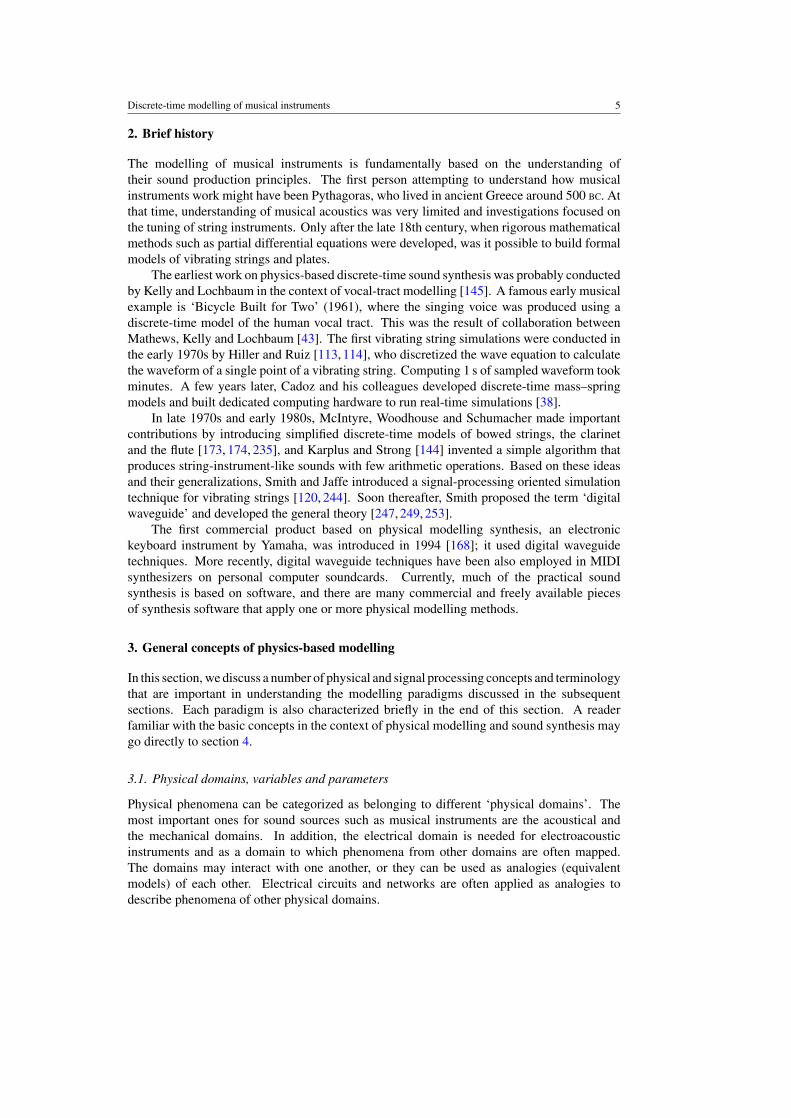
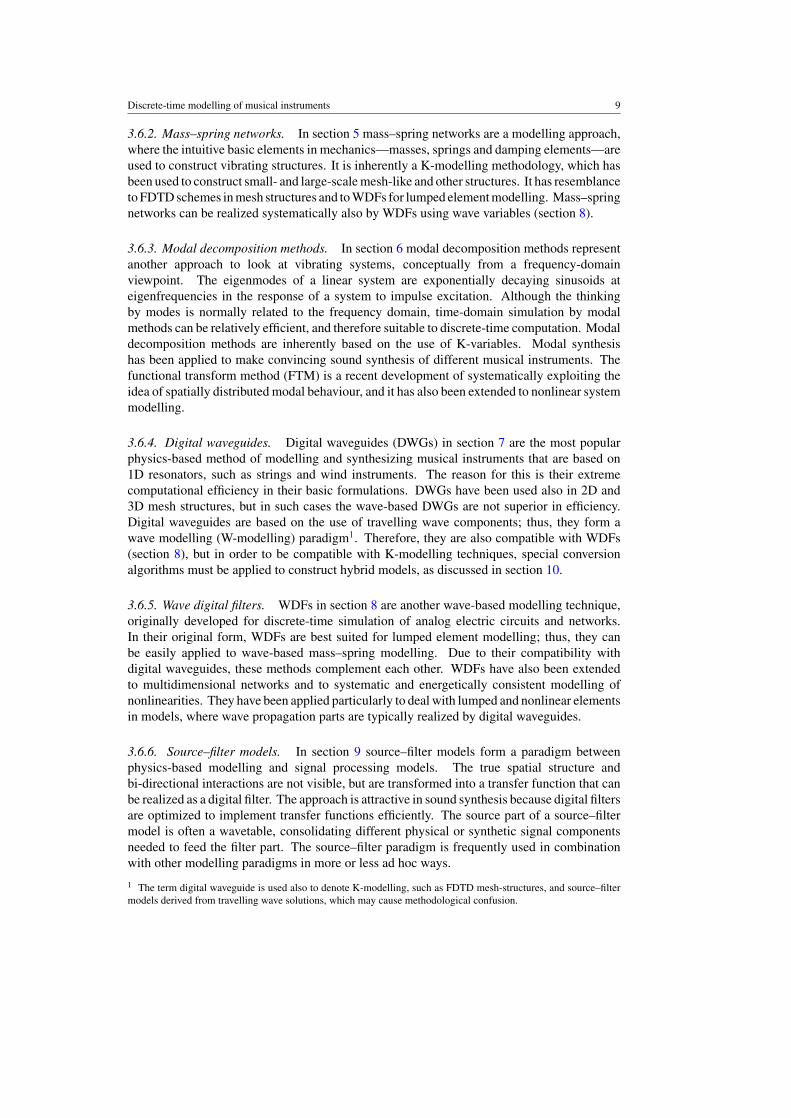
Figure 1. Part of an ideal vibrating string.

4. Finite difference models

The finite difference schemes can be used for solving partial differential equations, such asthose describing the vibration of a string, a membrane or an air column inside a tube [264].The key idea in the finite difference scheme is to replace derivatives with finite differenceapproximations. An early example of this approach in physical modelling of musicalinstruments is the work done by Hiller and Ruiz in the early 1970s [113, 114]. This line ofresearch has been continued and extended by Chaigne and colleagues [45,46,48] and recentlyby others [25, 26, 29, 30, 81, 103, 131].

The finite difference approach leads to a simulation algorithm that is based on a differenceequation, which can be easily programmed with a computer. As an example, let us seehow the basic wave equation, which describes the small-amplitude vibration of a lossless,ideally flexible string, is discretized using this principle. Here we present a formulation afterSmith [253] using an ideal string as a starting point for discrete-time modelling. A morethorough continuous-time analysis of the physics of strings can be found in [96].

4.1. Finite difference model for an ideal vibrating string

Figure 1 depicts a snapshot of an ideal (lossless, linear, flexible) vibrating string by showingthe displacement as a function of position.

The wave equation for the string is given by

Ky ′′ = εy, (1)

where the definitions for symbols are K = string tension (constant), ε = linearmass density (constant), y = y(t, x) = string displacement, y = (∂/∂t)y(t, x) = stringvelocity, y = (∂2/∂t2)y(t, x) = string acceleration, y ′ = (∂/∂x)y(t, x) = string slope andy ′′ = (∂2/∂x2)y(t, x) = string curvature.

Note that the derivation of equation (1) assumes that the string slope has a value muchless than 1 at all times and positions [96].

There are many techniques for approximating the partial differential terms with finitedifferences. The three most common replacements are the forward difference approximation,

f ′ ≈ f (x + �x) − f (x)

�x, (2)

the central difference approximation,

f ′ ≈ f (x + �x) − f (x − �x)

2�x(3)

and the backward difference approximation,

f ′ ≈ f (x) − f (x − �x)

�x. (4)

Discrete-time modelling of musical instruments 11

Tim

e

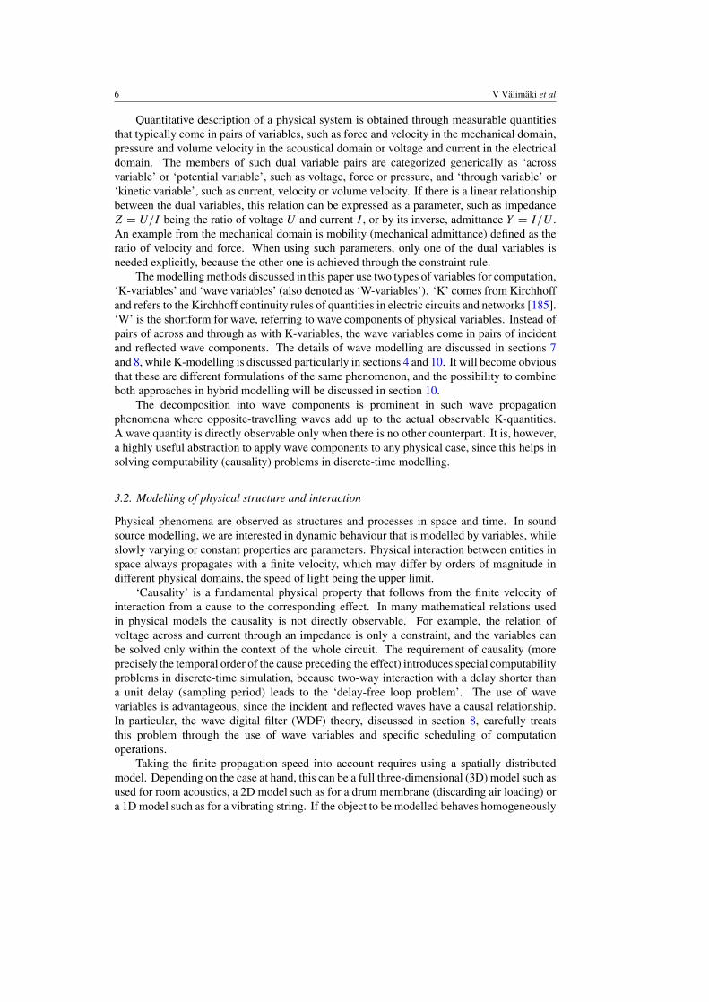
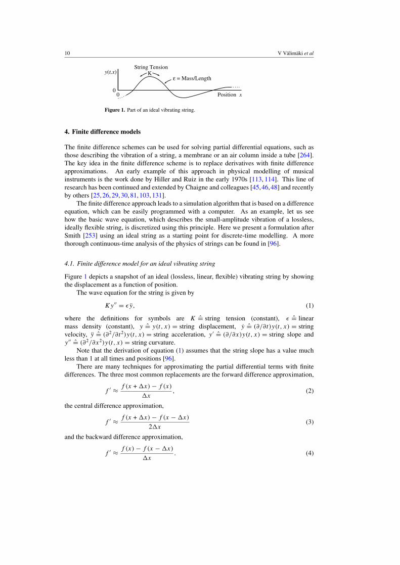
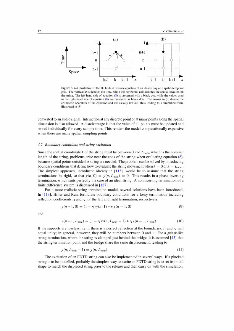
Figure 2. Block diagram of a finite difference approximation of the wave equation accordingto (8). The diagram shows how the next displacement value of the current position y(n + 1, k) iscomputed from the present values of its neighbours, y(n, k − 1) and y(n, k + 1), and the previousvalue y(n − 1, k). The block z−1 indicates a delay of one sampling interval.

Using the forward and backward difference approximations for the second partialderivatives and using indices n and k for the temporal and spatial points, respectively, yieldsthe following version of the wave equation:

y(n + 1, k) − 2y(n, k) + y(n − 1, k)

T 2= c2 y(n, k + 1) − 2y(n, k) + y(n, k − 1)

X2, (5)

where T and X are the temporal and spatial sampling intervals, respectively, and

c =√

K/ε (6)

is the propagation velocity of the transversal wave. We may select the spatial and the temporalsampling intervals so that

R = cX

T� 1, (7)

that is, the waves in the discrete model do not propagate faster than one spatial interval at eachtime step. Here, R is called the Courant number and the inequality is known as the Courant–Friedrichs–Levy condition. Interestingly, the Von Neumann stability analysis (see, e.g. [264])gives the same condition for R in the case of an ideal vibrating string. Now, by setting R = 1it is easy to write (5) in the form that shows how the next displacement value y(n + 1, k) iscomputed from the present and the past values:

y(n + 1, k) = y(n, k + 1) + y(n, k − 1) − y(n − 1, k). (8)

The recurrence equation (8) is also known as the leapfrog recursion. Figure 2 illustratesthis update rule as a signal-processing block diagram, as suggested by Karjalainen [127]. Thevalue of spatial index k increases to the right while the temporal index n increases upwards. Thediagram shows how the next displacement value of the current position y(n+1, k) is computedfrom the present values of its neighbours, y(n, k − 1) and y(n, k + 1), and the previous valuey(n − 1, k). The diagram also indicates that the update rule is the same for all elements.

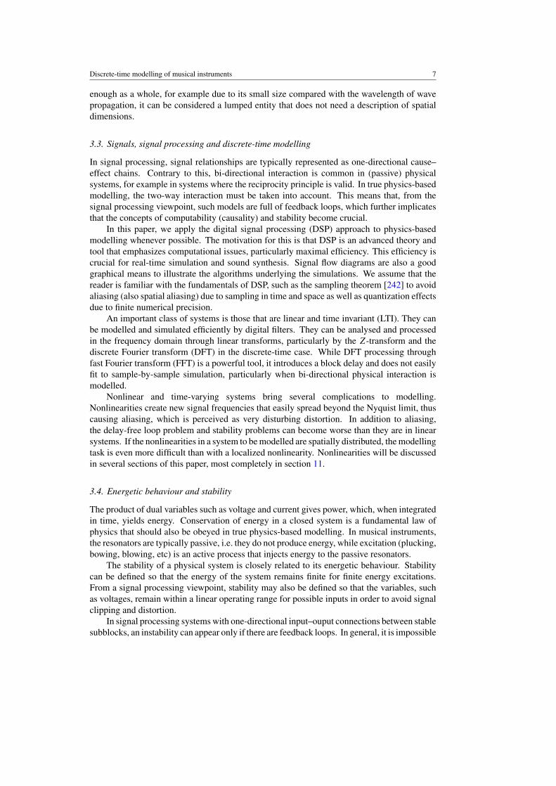
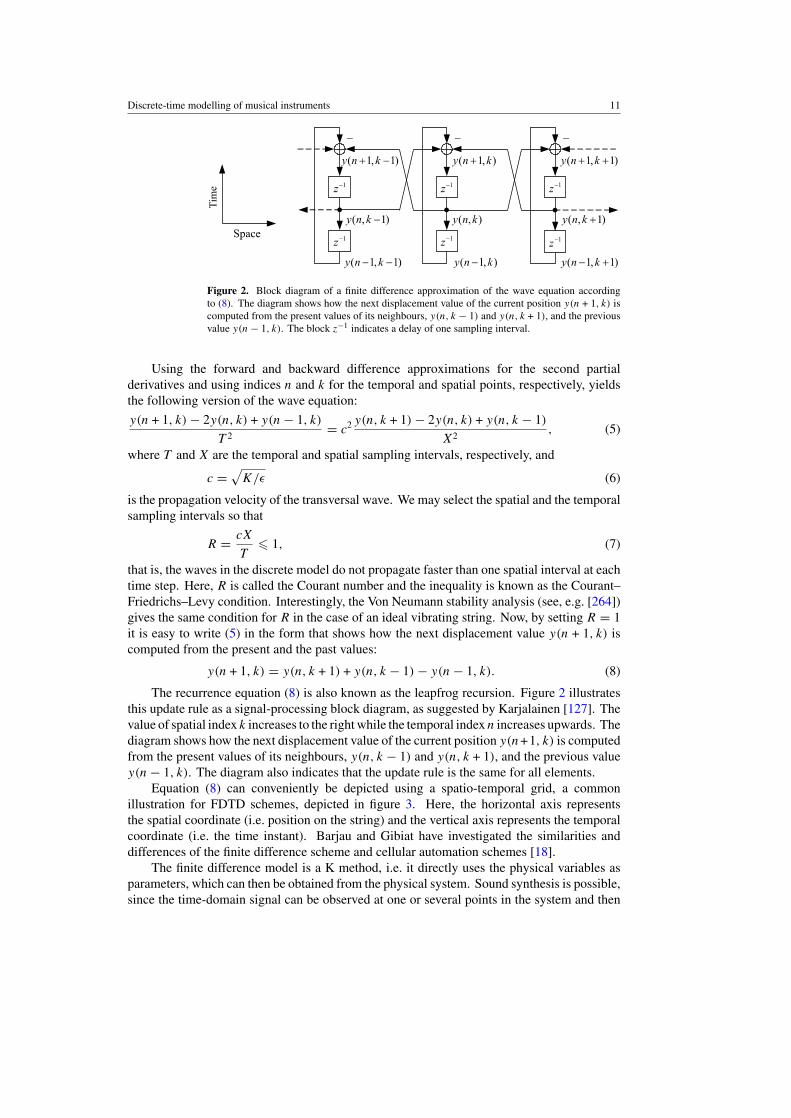
Equation (8) can conveniently be depicted using a spatio-temporal grid, a commonillustration for FDTD schemes, depicted in figure 3. Here, the horizontal axis representsthe spatial coordinate (i.e. position on the string) and the vertical axis represents the temporalcoordinate (i.e. the time instant). Barjau and Gibiat have investigated the similarities anddifferences of the finite difference scheme and cellular automation schemes [18].

The finite difference model is a K method, i.e. it directly uses the physical variables asparameters, which can then be obtained from the physical system. Sound synthesis is possible,since the time-domain signal can be observed at one or several points in the system and then

12 V Valimaki et al

Figure 3. (a) Illustration of the 1D finite difference equation of an ideal string on a spatio-temporalgrid. The vertical axis denotes the time, while the horizontal axis denotes the spatial location onthe string. The left-hand side of equation (8) is presented with a black dot, while the values usedin the right-hand side of equation (8) are presented as blank dots. The arrows in (a) denote thearithmetic operators of the equation and are usually left out, thus leading to a simplified form,illustrated in (b).

converted to an audio signal. Interaction at any discrete point or at many points along the spatialdimension is also allowed. A disadvantage is that the value of all points must be updated andstored individually for every sample time. This renders the model computationally expensivewhen there are many spatial sampling points.

4.2. Boundary conditions and string excitation

Since the spatial coordinate k of the string must lie between 0 and Lnom, which is the nominallength of the string, problems arise near the ends of the string when evaluating equation (8),because spatial points outside the string are needed. The problem can be solved by introducingboundary conditions that define how to evaluate the string movement when k = 0 or k = Lnom.The simplest approach, introduced already in [113], would be to assume that the stringterminations be rigid, so that y(n, 0) = y(n, Lnom) = 0. This results in a phase-invertingtermination, which suits perfectly the case of an ideal string. A noninverting termination of afinite difference system is discussed in [127].

For a more realistic string termination model, several solutions have been introduced.In [113], Hiller and Ruiz formulate boundary conditions for a lossy termination includingreflection coefficients rl and rr for the left and right termination, respectively,

y(n + 1, 0) = (1 − rl)y(n, 1) + rly(n − 1, 0) (9)

and

y(n + 1, Lnom) = (1 − rr)y(n, Lnom − 1) + rry(n − 1, Lnom). (10)

If the supports are lossless, i.e. if there is a perfect reflection at the boundaries, rl and rr willequal unity; in general, however, they will be numbers between 0 and 1. For a guitar-likestring termination, where the string is clamped just behind the bridge, it is assumed [45] thatthe string termination point and the bridge share the same displacement, leading to

y(n, Lnom − 1) = y(n, Lnom). (11)

The excitation of an FDTD string can also be implemented in several ways. If a pluckedstring is to be modelled, probably the simplest way to excite an FDTD string is to set its initialshape to match the displaced string prior to the release and then carry on with the simulation.

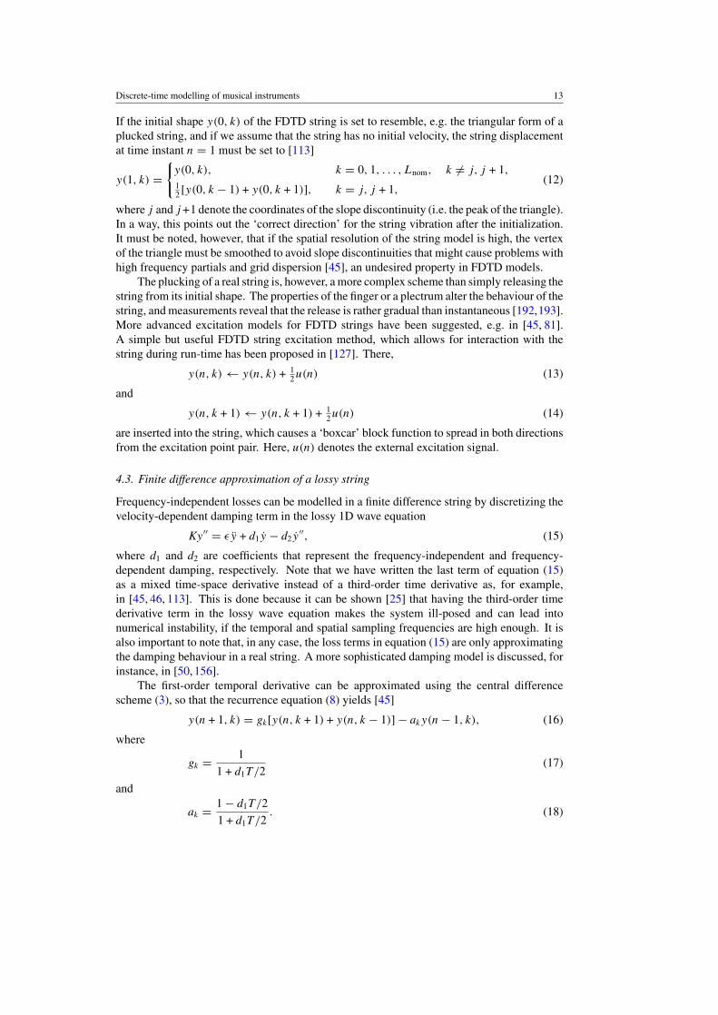
Discrete-time modelling of musical instruments 13

If the initial shape y(0, k) of the FDTD string is set to resemble, e.g. the triangular form of aplucked string, and if we assume that the string has no initial velocity, the string displacementat time instant n = 1 must be set to [113]

y(1, k) ={

y(0, k), k = 0, 1, . . . , Lnom, k �= j, j + 1,

12 [y(0, k − 1) + y(0, k + 1)], k = j, j + 1,

(12)

where j and j +1 denote the coordinates of the slope discontinuity (i.e. the peak of the triangle).In a way, this points out the ‘correct direction’ for the string vibration after the initialization.It must be noted, however, that if the spatial resolution of the string model is high, the vertexof the triangle must be smoothed to avoid slope discontinuities that might cause problems withhigh frequency partials and grid dispersion [45], an undesired property in FDTD models.

The plucking of a real string is, however, a more complex scheme than simply releasing thestring from its initial shape. The properties of the finger or a plectrum alter the behaviour of thestring, and measurements reveal that the release is rather gradual than instantaneous [192,193].More advanced excitation models for FDTD strings have been suggested, e.g. in [45, 81].A simple but useful FDTD string excitation method, which allows for interaction with thestring during run-time has been proposed in [127]. There,

y(n, k) ← y(n, k) + 12u(n) (13)

and

y(n, k + 1) ← y(n, k + 1) + 12u(n) (14)

are inserted into the string, which causes a ‘boxcar’ block function to spread in both directionsfrom the excitation point pair. Here, u(n) denotes the external excitation signal.

4.3. Finite difference approximation of a lossy string

Frequency-independent losses can be modelled in a finite difference string by discretizing thevelocity-dependent damping term in the lossy 1D wave equation

Ky ′′ = εy + d1y − d2y′′, (15)

where d1 and d2 are coefficients that represent the frequency-independent and frequency-dependent damping, respectively. Note that we have written the last term of equation (15)as a mixed time-space derivative instead of a third-order time derivative as, for example,in [45, 46, 113]. This is done because it can be shown [25] that having the third-order timederivative term in the lossy wave equation makes the system ill-posed and can lead intonumerical instability, if the temporal and spatial sampling frequencies are high enough. It isalso important to note that, in any case, the loss terms in equation (15) are only approximatingthe damping behaviour in a real string. A more sophisticated damping model is discussed, forinstance, in [50, 156].

The first-order temporal derivative can be approximated using the central differencescheme (3), so that the recurrence equation (8) yields [45]

y(n + 1, k) = gk[y(n, k + 1) + y(n, k − 1)] − aky(n − 1, k), (16)

where

gk = 1

1 + d1T/2(17)

and

ak = 1 − d1T/2

1 + d1T/2. (18)

14 V Valimaki et al

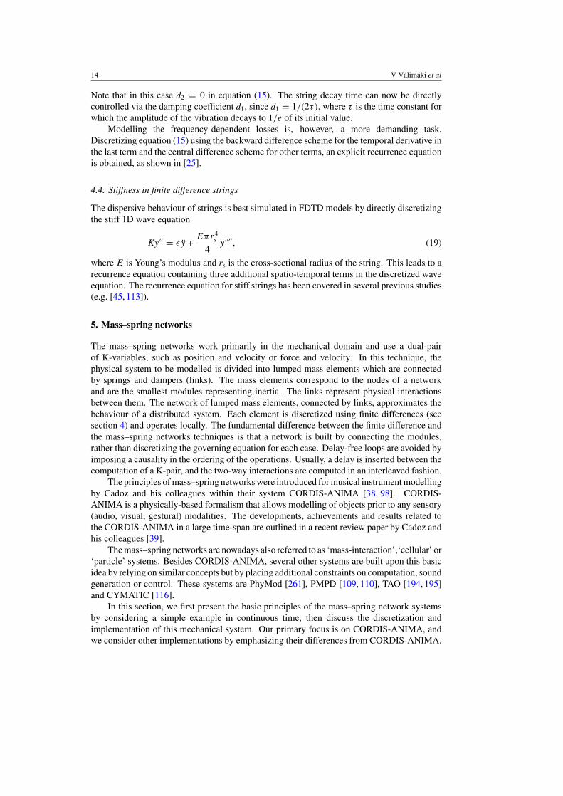
Note that in this case d2 = 0 in equation (15). The string decay time can now be directlycontrolled via the damping coefficient d1, since d1 = 1/(2τ), where τ is the time constant forwhich the amplitude of the vibration decays to 1/e of its initial value.

Modelling the frequency-dependent losses is, however, a more demanding task.Discretizing equation (15) using the backward difference scheme for the temporal derivative inthe last term and the central difference scheme for other terms, an explicit recurrence equationis obtained, as shown in [25].

4.4. Stiffness in finite difference strings

The dispersive behaviour of strings is best simulated in FDTD models by directly discretizingthe stiff 1D wave equation

Ky ′′ = εy +Eπr4

s

4y ′′′′, (19)

where E is Young’s modulus and rs is the cross-sectional radius of the string. This leads to arecurrence equation containing three additional spatio-temporal terms in the discretized waveequation. The recurrence equation for stiff strings has been covered in several previous studies(e.g. [45, 113]).

5. Mass–spring networks

The mass–spring networks work primarily in the mechanical domain and use a dual-pairof K-variables, such as position and velocity or force and velocity. In this technique, thephysical system to be modelled is divided into lumped mass elements which are connectedby springs and dampers (links). The mass elements correspond to the nodes of a networkand are the smallest modules representing inertia. The links represent physical interactionsbetween them. The network of lumped mass elements, connected by links, approximates thebehaviour of a distributed system. Each element is discretized using finite differences (seesection 4) and operates locally. The fundamental difference between the finite difference andthe mass–spring networks techniques is that a network is built by connecting the modules,rather than discretizing the governing equation for each case. Delay-free loops are avoided byimposing a causality in the ordering of the operations. Usually, a delay is inserted between thecomputation of a K-pair, and the two-way interactions are computed in an interleaved fashion.

The principles of mass–spring networks were introduced for musical instrument modellingby Cadoz and his colleagues within their system CORDIS-ANIMA [38, 98]. CORDIS-ANIMA is a physically-based formalism that allows modelling of objects prior to any sensory(audio, visual, gestural) modalities. The developments, achievements and results related tothe CORDIS-ANIMA in a large time-span are outlined in a recent review paper by Cadoz andhis colleagues [39].

The mass–spring networks are nowadays also referred to as ‘mass-interaction’,‘cellular’ or‘particle’ systems. Besides CORDIS-ANIMA, several other systems are built upon this basicidea by relying on similar concepts but by placing additional constraints on computation, soundgeneration or control. These systems are PhyMod [261], PMPD [109, 110], TAO [194, 195]and CYMATIC [116].

In this section, we first present the basic principles of the mass–spring network systemsby considering a simple example in continuous time, then discuss the discretization andimplementation of this mechanical system. Our primary focus is on CORDIS-ANIMA, andwe consider other implementations by emphasizing their differences from CORDIS-ANIMA.

Discrete-time modelling of musical instruments 15

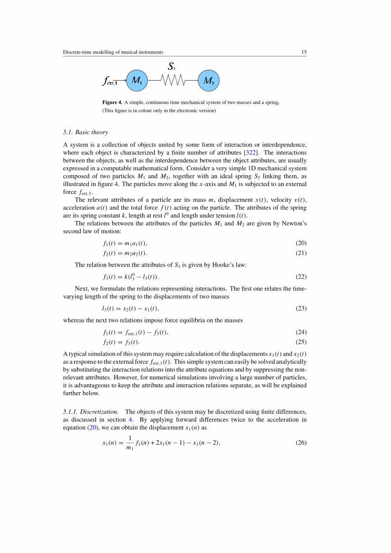
Figure 4. A simple, continuous time mechanical system of two masses and a spring.

(This figure is in colour only in the electronic version)

5.1. Basic theory

A system is a collection of objects united by some form of interaction or interdependence,where each object is characterized by a finite number of attributes [322]. The interactionsbetween the objects, as well as the interdependence between the object attributes, are usuallyexpressed in a computable mathematical form. Consider a very simple 1D mechanical systemcomposed of two particles M1 and M2, together with an ideal spring S3 linking them, asillustrated in figure 4. The particles move along the x-axis and M1 is subjected to an externalforce fext,1.

The relevant attributes of a particle are its mass m, displacement x(t), velocity v(t),acceleration a(t) and the total force f (t) acting on the particle. The attributes of the springare its spring constant k, length at rest l0 and length under tension l(t).

The relations between the attributes of the particles M1 and M2 are given by Newton’ssecond law of motion:

f1(t) = m1a1(t), (20)

f2(t) = m2a2(t). (21)

The relation between the attributes of S3 is given by Hooke’s law:

f3(t) = k(l03 − l3(t)). (22)

Next, we formulate the relations representing interactions. The first one relates the time-varying length of the spring to the displacements of two masses

l3(t) = x2(t) − x1(t), (23)

whereas the next two relations impose force equilibria on the masses

f1(t) = fext,1(t) − f3(t), (24)

f2(t) = f3(t). (25)

A typical simulation of this system may require calculation of the displacements x1(t) and x2(t)

as a response to the external force fext,1(t). This simple system can easily be solved analyticallyby substituting the interaction relations into the attribute equations and by suppressing the non-relevant attributes. However, for numerical simulations involving a large number of particles,it is advantageous to keep the attribute and interaction relations separate, as will be explainedfurther below.

5.1.1. Discretization. The objects of this system may be discretized using finite differences,as discussed in section 4. By applying forward differences twice to the acceleration inequation (20), we can obtain the displacement x1(n) as

x1(n) = 1

m1f1(n) + 2x1(n − 1) − x1(n − 2), (26)

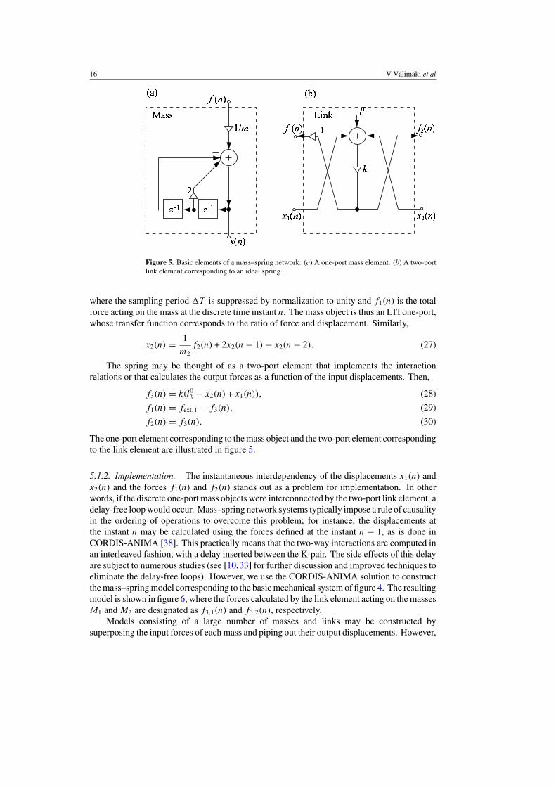
16 V Valimaki et al

Figure 5. Basic elements of a mass–spring network. (a) A one-port mass element. (b) A two-portlink element corresponding to an ideal spring.

where the sampling period �T is suppressed by normalization to unity and f1(n) is the totalforce acting on the mass at the discrete time instant n. The mass object is thus an LTI one-port,whose transfer function corresponds to the ratio of force and displacement. Similarly,

x2(n) = 1

m2f2(n) + 2x2(n − 1) − x2(n − 2). (27)

The spring may be thought of as a two-port element that implements the interactionrelations or that calculates the output forces as a function of the input displacements. Then,

f3(n) = k(l03 − x2(n) + x1(n)), (28)

f1(n) = fext,1 − f3(n), (29)

f2(n) = f3(n). (30)

The one-port element corresponding to the mass object and the two-port element correspondingto the link element are illustrated in figure 5.

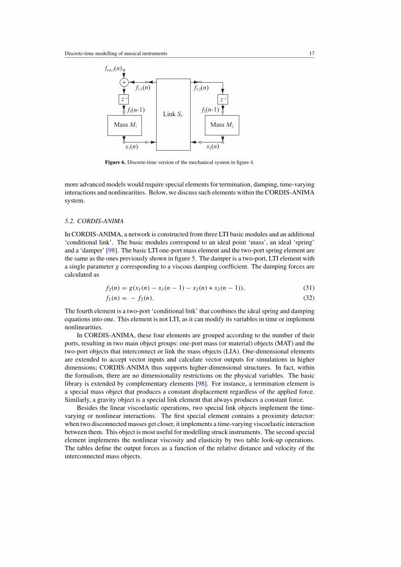
5.1.2. Implementation. The instantaneous interdependency of the displacements x1(n) andx2(n) and the forces f1(n) and f2(n) stands out as a problem for implementation. In otherwords, if the discrete one-port mass objects were interconnected by the two-port link element, adelay-free loop would occur. Mass–spring network systems typically impose a rule of causalityin the ordering of operations to overcome this problem; for instance, the displacements atthe instant n may be calculated using the forces defined at the instant n − 1, as is done inCORDIS-ANIMA [38]. This practically means that the two-way interactions are computed inan interleaved fashion, with a delay inserted between the K-pair. The side effects of this delayare subject to numerous studies (see [10,33] for further discussion and improved techniques toeliminate the delay-free loops). However, we use the CORDIS-ANIMA solution to constructthe mass–spring model corresponding to the basic mechanical system of figure 4. The resultingmodel is shown in figure 6, where the forces calculated by the link element acting on the massesM1 and M2 are designated as f3,1(n) and f3,2(n), respectively.

Models consisting of a large number of masses and links may be constructed bysuperposing the input forces of each mass and piping out their output displacements. However,

Discrete-time modelling of musical instruments 17

Mass M1

z -1

fext,1(n)

Link S3

f3,1(n)

Mass M2

z -1

f3,2(n)

f1(n-1) f2(n-1)

x1(n) x2(n)

Figure 6. Discrete-time version of the mechanical system in figure 4.

more advanced models would require special elements for termination, damping, time-varyinginteractions and nonlinearities. Below, we discuss such elements within the CORDIS-ANIMAsystem.

5.2. CORDIS-ANIMA

In CORDIS-ANIMA, a network is constructed from three LTI basic modules and an additional‘conditional link’. The basic modules correspond to an ideal point ‘mass’, an ideal ‘spring’and a ‘damper’ [98]. The basic LTI one-port mass element and the two-port spring element arethe same as the ones previously shown in figure 5. The damper is a two-port, LTI element witha single parameter g corresponding to a viscous damping coefficient. The damping forces arecalculated as

f2(n) = g(x1(n) − x1(n − 1) − x2(n) + x2(n − 1)), (31)

f1(n) = − f2(n). (32)

The fourth element is a two-port ‘conditional link’ that combines the ideal spring and dampingequations into one. This element is not LTI, as it can modify its variables in time or implementnonlinearities.

In CORDIS-ANIMA, these four elements are grouped according to the number of theirports, resulting in two main object groups: one-port mass (or material) objects (MAT) and thetwo-port objects that interconnect or link the mass objects (LIA). One-dimensional elementsare extended to accept vector inputs and calculate vector outputs for simulations in higherdimensions; CORDIS-ANIMA thus supports higher-dimensional structures. In fact, withinthe formalism, there are no dimensionality restrictions on the physical variables. The basiclibrary is extended by complementary elements [98]. For instance, a termination element isa special mass object that produces a constant displacement regardless of the applied force.Similarly, a gravity object is a special link element that always produces a constant force.

Besides the linear viscoelastic operations, two special link objects implement the time-varying or nonlinear interactions. The first special element contains a proximity detector:when two disconnected masses get closer, it implements a time-varying viscoelastic interactionbetween them. This object is most useful for modelling struck instruments. The second specialelement implements the nonlinear viscosity and elasticity by two table look-up operations.The tables define the output forces as a function of the relative distance and velocity of theinterconnected mass objects.

18 V Valimaki et al

The CORDIS-ANIMA library is further extended by prepackaged modules. Some ofthese modules support other synthesis paradigms, such as modal synthesis or basic digitalwaveguides. Constructing a detailed mass-interaction network is still a non-trivial task, sincethe objects and their interconnection topology require a large number of parameters. Cadozand his colleagues, therefore, have developed support systems for mass-interaction networks.These systems include the model authoring environment GENESIS [42] (a user-interfacededicated to musical applications of CORDIS-ANIMA), the visualization environmentMIMESIS [39] (an environment dedicated to the production of animated images) and tools foranalysis and parameter estimation [270].

A large number of audio–visual modelling examples is reported in [39]. These examplesinclude a model of a six-wheel vehicle interacting with soil, simple animal models such asfrogs and snakes and models of collective behaviour within a large ensemble of particles.The most advanced model for sound synthesis by mass-interaction networks (and probablyby any physics-based algorithm) is the model that creates the musical piece ‘pico..TERA’,which was developed by Cadoz using the CORDIS-ANIMA and GENESIS systems [36]. Inthis model, thousands of particles and many aggregate geometrical objects interact with eachother. The 290 s of music is synthesized by running this model without any external interactionor post-processing.

5.3. Other mass–spring systems

PhyMod [261] is an early commercial software for visualization and sound synthesis ofmass–spring structures. Besides the 1D mass and linear link objects, four nonlinear linkelements are provided. The program uses a visual interface for building a sound sculpturefrom elementary objects. The basic algorithmic principles of this system (but not its visualinterface) has been ported to the popular csound environment [56].

The system PMPD2 [109, 110] closely follows the CORDIS-ANIMA formulation forvisualization of mass-interaction networks within the pd-GEM environment [206]. In additionto the masses and links in one or more dimensions, PMPD defines higher-level aggregategeometrical objects such as squares and circles in 2D or cubes or spheres in 3D. The PMPDpackage also contains examples for 2D and 3D vibrations of a linear elastic string in itsdocumentation subfolder (example 5: corde2D and example 7: corde3D). Although the packageis a very valuable tool for understanding the basic principles or mass-interaction networks, ithas limited support for audio synthesis.

TAO3 specifically addresses the difficulty of model construction and the lack of a scriptinglanguage in the CORDIS-ANIMA system [194, 195]. It uses a fixed topology of masses andsprings and provides pre-constructed 1D (string) or 2D (triangle, rectangle, circle and ellipse)modules, but 3D modules are not supported. Operations such as deleting the mass objects forconstructing shapes with holes and joining the shapes are defined. For efficiency and reductionin the number of parameters, TAO constrains the spring objects by using a fixed spring constant.The system is driven by a score; the audio output is picked-up by virtual microphones andstreamed to a file, which is normalized when the stream finishes.

A real-time synthesis software called CYMATIC was recently developed by Howard andRimell [116]. The synthesis engine of CYMATIC is based on TAO, but it introduces twoimportant improvements. The first improvement is the replacement of the forward differences

2 PMPD has multi-platform support and it is released as a free software under the GNU Public License (GPL). It canbe downloaded from http://drpichon.free.fr/pmpd/.3 TAO is an active software development project and it is released as a free software under the GPL. It resides athttp://sourceforge.net/projects/taopm/.

Discrete-time modelling of musical instruments 19

Figure 7. Schematic presentation of the modal synthesis method.

common in all previous systems by central differences. The central difference scheme resultsin a more stable model and reduces the frequency warping. The second improvement inCYMATIC over TAO is the support for 3D structures, as in CORDIS-ANIMA and PMPD.

6. Modal decomposition methods

Modal decomposition describes a linear system in terms of its modes of vibration. Modellingmethods based on this approach look at the vibrating structure from the frequency point of view,because modes are essentially a spectral property of a sound source. Nevertheless, physicalmodels based on modal decomposition lead to discrete-time algorithms that compute the valueof the output signal of the simulation at each sampling step. In this sense, modal methods havemuch in common with other discrete-time modelling techniques discussed in this paper. In thissection, we give an overview of the modal synthesis, some filter-based modal decompositionmethods and the FTM.

6.1. Modal synthesis

An early application of the modal decomposition method to modelling of musical instrumentsand sound synthesis was developed by Adrien at IRCAM [2, 3]. In his work, eachvibrating mode had a resonance frequency, damping factor and physical shape specified ona discrete grid. The synthesis was strongly related to vibration measurements of a specificstructure or instrument, and this is where the modal data was obtained. A software productcalled Modalys (formerly MOSAIC) by IRCAM is based on modal synthesis [78, 178].Bisnovatyi has developed another software-based system for experimenting with real-timemodal synthesis [32].

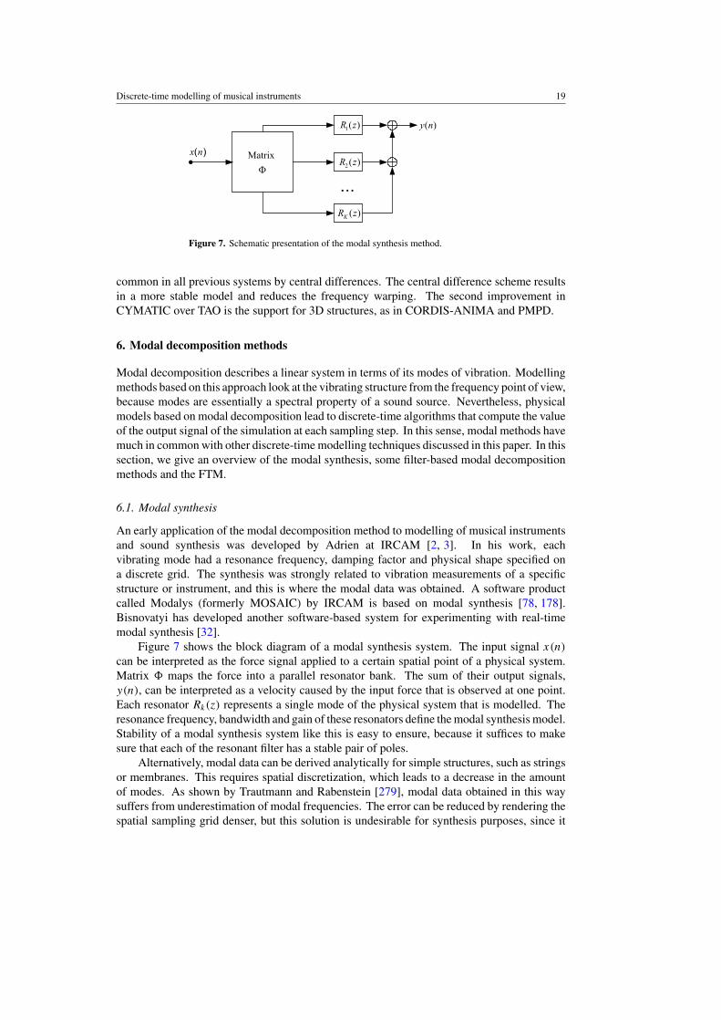
Figure 7 shows the block diagram of a modal synthesis system. The input signal x(n)

can be interpreted as the force signal applied to a certain spatial point of a physical system.Matrix � maps the force into a parallel resonator bank. The sum of their output signals,y(n), can be interpreted as a velocity caused by the input force that is observed at one point.Each resonator Rk(z) represents a single mode of the physical system that is modelled. Theresonance frequency, bandwidth and gain of these resonators define the modal synthesis model.Stability of a modal synthesis system like this is easy to ensure, because it suffices to makesure that each of the resonant filter has a stable pair of poles.

Alternatively, modal data can be derived analytically for simple structures, such as stringsor membranes. This requires spatial discretization, which leads to a decrease in the amountof modes. As shown by Trautmann and Rabenstein [279], modal data obtained in this waysuffers from underestimation of modal frequencies. The error can be reduced by rendering thespatial sampling grid denser, but this solution is undesirable for synthesis purposes, since it

20 V Valimaki et al

increases the number of modes and thus the computational cost becomes larger. An obviousway to reduce the computational cost of real-time modal synthesis is to prune the number ofmodes by leaving out some resonant filters.

6.2. Filter-based modal methods

Another approach to modal synthesis that is well suited for percussive sounds, such as drumsor bells, is to extract modal data from a recorded signal. Various signal-processing methodsare known that can estimate a digital filter transfer function for a given sampled signal. Sandlerused linear prediction techniques [223, 224] and Mackenzie et al applied the balanced modeltruncation method [166] to obtain a digital filter model for drum sounds. Laroche [158]and Macon et al [167] applied parametric methods on various frequency bands for the sametask. The frequency-zooming ARMA method [133] can yield a high-resolution parametricfilter model for acoustic signals even if they have a large number of modes located close toeach other in frequency. While all such filter models allow accurate modelling and flexiblemodification of each resonance, they are less meaningful physically than analytically derivedor measurement-based modal synthesis models, since they lack information about the spatialdistribution of the modes.

Laroche and Meillier [159] proposed a parametric synthesis model for the piano basedon a modal resonator bank. This approach allows exact adjustment of the frequency, thelevel and the decay rate for each mode of a vibrating string, which is helpful for imitatingthe inharmonicity and complex temporal decay patterns of partials observed in piano tones.State–space modelling discussed by Matignon et al [170,171] and by Depalle and Tassart [74]is another approach to derive filter-based models. The resulting transfer function can beimplemented with modal resonant filters or as a high order digital filter. The coupled modesynthesis technique introduced by Van Duyne [297] is another filter-based approach to modalsynthesis. It has a special filter structure in which allpass filters are used as building blocksand they are all fed back through the same filter. Banded waveguides introduced by Esslet al [86–90] combine characteristics from modal synthesis and digital waveguides, which wediscuss in section 7.

Cook has extended the idea of modal synthesis to parametric synthesis of percussivesounds with noisy excitation [63,66]. This method is called physical inspired sonic modellingor PhISM. Based on parametric spectral analysis, the PhISM method derives a resonator bankand an associated excitation signal. From analysis of several types of excitation it is possibleto parametrize the strike position and style, which can then be used for real-time control. Theinput signal for synthesis can be obtained, for example, by inverse filtering and by simplifyingthe residual signal. Inverse filtering in this case refers to the process of filtering a recordedsignal using the inverted transfer function of the resonant filter bank.

The filter-based modal synthesis methods can be called source–filter models, since theyconsist in essence of a filter transfer function and a properly chosen input signal. Source–filtermodels are discussed in section 9 of this paper.

6.3. The functional transform method

A novel technique related to modal synthesis is the FTM introduced by Trautmann andRabenstein [207, 278, 279], which also describes a linear system in terms of its modes.This method allows the derivation of accurate models based directly on physics for simplegeometries, just as can be done with finite difference models. The main novelty in functionaltransform modelling is to apply two different integral transforms to remove partial derivatives.

Discrete-time modelling of musical instruments 21

The Laplace transform operates on the temporal and the Sturm–Liouville transform on thespatial terms of the partial differential equation. The multidimensional transfer function canthen be implemented using digital filters. For linear systems, this results in a set of second-orderresonators connected in parallel, just as shown in figure 7. The method can also be extendedfor nonlinear systems [279, 280]. The FTM can be used for constructing accurate physicalmodels of vibrating strings and membranes without conducting physical measurements, if thenecessary numerical values of physical variables are known. Advantages of this modellingmethod are that spatial discretization is unnecessary, that there is no systematic error in modefrequencies and that the signal phase is correct with respect to both the input and the outputlocations [279].

7. Digital waveguides

The digital waveguide (DWG) method is based on discrete-time modelling of the propagationand scattering of waves. The principle was used already in the Kelly–Lochbaum speechsynthesis model [145, 266], in which the human vocal tract was simulated by unit-sampledelay lines and wave scattering junctions between them. Such modelling has often been called‘transmission-line modelling’, but in computer music it is better known by the term ‘digitalwaveguide modelling’. This term was proposed by Smith [245, 247] because of an analogyto the concept of waveguide that has been used, for example, in microwave technology. Foralmost two decades, DWGs have been the most popular and successful physics-based modellingmethodology, particularly for efficient sound synthesis applications [249, 253, 254].

In this section, we present an overview of digital waveguide modelling, deriving fromthe behaviour of plucked strings and acoustic tubes, but also discussing modelling of otherinstruments. Relations of DWGs to other modelling paradigms are mentioned briefly. Somestructures, such as extensions of the Karplus–Strong model, can be seen as intermediate casesbetween DWGs and source–filter models. Although they may seem to belong more to thesource–filter category (section 9), in this presentation they are discussed primarily in thepresent section on digital waveguides.

7.1. From wave propagation to digital waveguides

A vibrating string is a good example of one-dimensional wave propagation that can serve forderivation of the digital waveguide principle. Here we present a formulation after Smith [253]using an ideal string as a starting point for discrete-time modelling. A more thoroughcontinuous-time analysis of the physics of strings can be found, for example, in [96].

The derivation of digital waveguides can be started from figure 1 and the same waveequation as for the finite difference models in section 4, i.e.

Ky ′′ = εy. (33)

It can be readily checked that any string shape that travels to the left or right with speedc = √

K/ε is a solution to the wave equation. If we denote right-going travelling waves byyr(x − ct) and left-going travelling waves by yl(x + ct), where yr and yl are arbitrary twice-differentiable functions, then the general class of solutions to the lossless, one-dimensional,second-order wave equation (33) can be expressed as

y(x, t) = yr(x − ct) + yl(x + ct), (34)

or, when time is the primary variable for expressing the signals,

y(t, x) = yr(t − x/c) + yl(t + x/c). (35)

22 V Valimaki et al

These forms, composed of opposite-travelling wave components of arbitrary waveforms, arecalled the d’Alembert solution of the wave equation. Assuming that signals yr and yl inequation (35) are bandlimited to one half of the sampling rate, we may sample the travellingwaves without losing any information. This yields

y(tn, xk) = yr(tn − xk/c) + yl(tn + xk/c)

= yr(nT − kX/c) + yl(nT + kX/c)

= yr[(n − k)T ] + yl[(n + k)T ], (36)

where T is the time interval and X the spatial interval between samples so that T = X/c.Sampling is applied in a discrete space-time grid in which indices n and k are related to timeand position, respectively. Since T multiplies all arguments, we suppress it by defining

y+(m) = yr(mT ) and y−(k) = yl(mT ). (37)

The ‘+’ superscript denotes a travelling wave component propagating to the right and ‘−’denotes propagation to the left. Finally, the left- and right-going travelling waves must besummed to produce a physical output according to the formula

y(tn, xk) = y+(n − k) + y−(n + k). (38)

The next step is to make the model more realistic by including losses and dispersion that appearin real strings.

7.2. Modelling of losses and dispersion

By adding proper derivatives of time, space or mixed time and space of different orders to thewave equation, the damping and dispersion of travelling waves in the string can be specified.For example the first-order spatial derivative (velocity) can control losses and the fourth-orderspatial derivative introduces dispersion, i.e. frequency-dependent wave velocity. Details onthe physics of string vibration damping are analysed, for example, in [282].

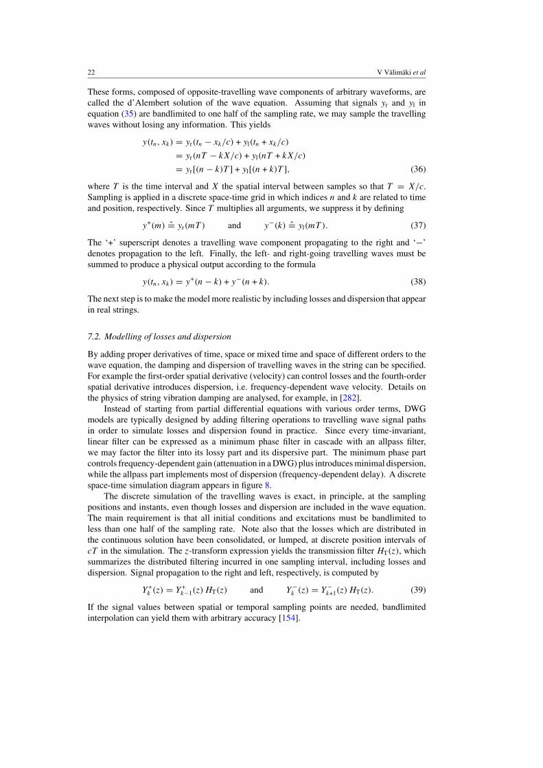
Instead of starting from partial differential equations with various order terms, DWGmodels are typically designed by adding filtering operations to travelling wave signal pathsin order to simulate losses and dispersion found in practice. Since every time-invariant,linear filter can be expressed as a minimum phase filter in cascade with an allpass filter,we may factor the filter into its lossy part and its dispersive part. The minimum phase partcontrols frequency-dependent gain (attenuation in a DWG) plus introduces minimal dispersion,while the allpass part implements most of dispersion (frequency-dependent delay). A discretespace-time simulation diagram appears in figure 8.

The discrete simulation of the travelling waves is exact, in principle, at the samplingpositions and instants, even though losses and dispersion are included in the wave equation.The main requirement is that all initial conditions and excitations must be bandlimited toless than one half of the sampling rate. Note also that the losses which are distributed inthe continuous solution have been consolidated, or lumped, at discrete position intervals ofcT in the simulation. The z-transform expression yields the transmission filter HT(z), whichsummarizes the distributed filtering incurred in one sampling interval, including losses anddispersion. Signal propagation to the right and left, respectively, is computed by

Y +k (z) = Y +

k−1(z) HT(z) and Y−k (z) = Y−

k+1(z) HT(z). (39)

If the signal values between spatial or temporal sampling points are needed, bandlimitedinterpolation can yield them with arbitrary accuracy [154].

Discrete-time modelling of musical instruments 23

Figure 8. Wave propagation simulated by a digital waveguide consisting of two delay lines forwave components travelling in opposite directions. Each delay line is a sequence of unit delays(z−1) and transmission filters HT(z) for losses and dispersion.

Figure 9. Digital waveguide obtained from the digital waveguide of figure 8 by consolidatingM unit delays and transmission filters in each delay line.

For computational efficiency reasons, the digital waveguide can be simplified by furtherconsolidation of elements between points of interest. Figure 9 shows how m consecutive delay-line sections can be combined into a single delay of M samples and transmission transferfunction HM

T (z). This helps for time-domain simulation and sound synthesis, making theDWG approach highly efficient.

7.3. Modelling of waveguide termination and scattering

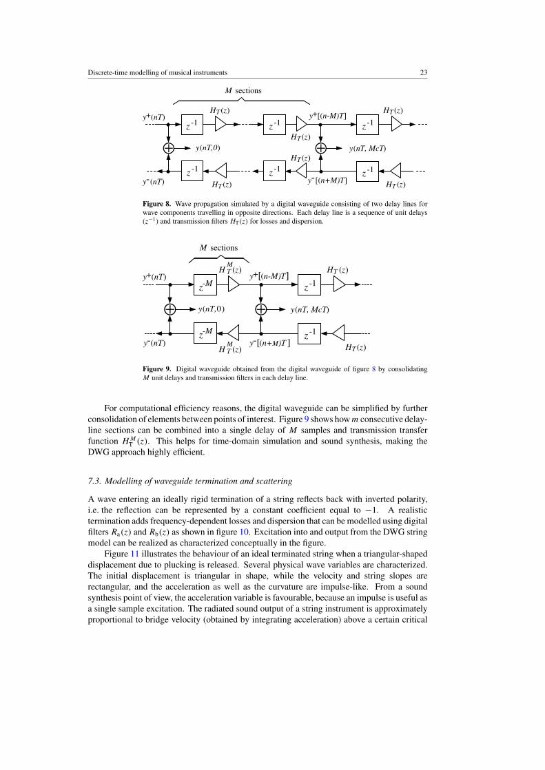
A wave entering an ideally rigid termination of a string reflects back with inverted polarity,i.e. the reflection can be represented by a constant coefficient equal to −1. A realistictermination adds frequency-dependent losses and dispersion that can be modelled using digitalfilters Ra(z) and Rb(z) as shown in figure 10. Excitation into and output from the DWG stringmodel can be realized as characterized conceptually in the figure.

Figure 11 illustrates the behaviour of an ideal terminated string when a triangular-shapeddisplacement due to plucking is released. Several physical wave variables are characterized.The initial displacement is triangular in shape, while the velocity and string slopes arerectangular, and the acceleration as well as the curvature are impulse-like. From a soundsynthesis point of view, the acceleration variable is favourable, because an impulse is useful asa single sample excitation. The radiated sound output of a string instrument is approximatelyproportional to bridge velocity (obtained by integrating acceleration) above a certain critical

24 V Valimaki et al

Delay line

Delay line

Rb(z)Ra(z)0.5Excitation Output

⊕

Figure 10. DWG model of a terminated string. Reflections of waves at terminations are representedby transfer functions Ra(z) and Rb(z). String input excitation and output probing are also shownconceptually.

(a) Displacement (c) Acceleration

Pluck point

(e) Curvature

Pp Pp

pp pp

(d) Slope

Figure 11. The behaviour of different mechanical waves in an ideal terminated string at the momentof plucking release: (a) displacement, (b) velocity, (c) acceleration, (d) slope and (e) curvature.

frequency, below which the radiation is proportional to acceleration. This is an idealizeddescription, whereby the detailed instrument body effects are also omitted.

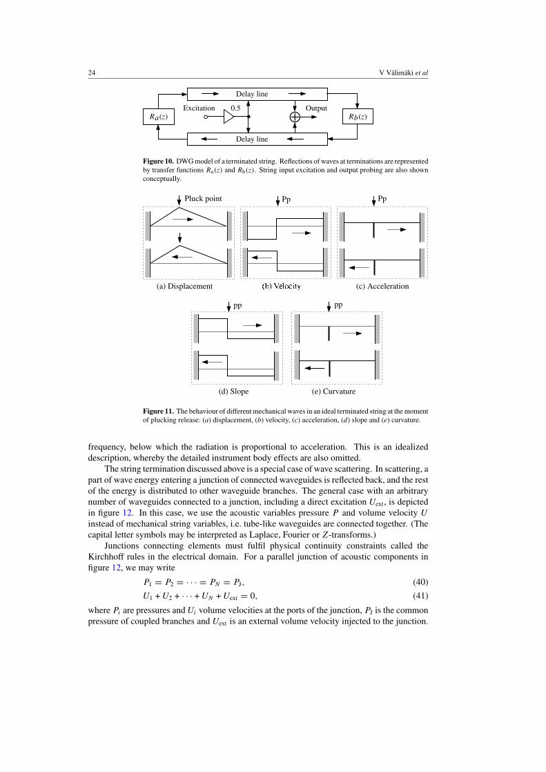
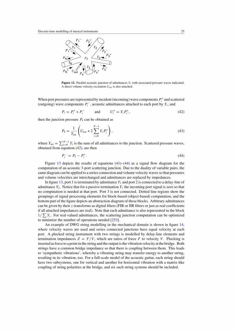
The string termination discussed above is a special case of wave scattering. In scattering, apart of wave energy entering a junction of connected waveguides is reflected back, and the restof the energy is distributed to other waveguide branches. The general case with an arbitrarynumber of waveguides connected to a junction, including a direct excitation Uext, is depictedin figure 12. In this case, we use the acoustic variables pressure P and volume velocity U

instead of mechanical string variables, i.e. tube-like waveguides are connected together. (Thecapital letter symbols may be interpreted as Laplace, Fourier or Z-transforms.)

Junctions connecting elements must fulfil physical continuity constraints called theKirchhoff rules in the electrical domain. For a parallel junction of acoustic components infigure 12, we may write

P1 = P2 = · · · = PN = PJ, (40)

U1 + U2 + · · · + UN + Uext = 0, (41)

where Pi are pressures and Ui volume velocities at the ports of the junction, PJ is the commonpressure of coupled branches and Uext is an external volume velocity injected to the junction.

Discrete-time modelling of musical instruments 25

P1–

PN–

P1+

PN+ Uext

pJ

P2–

P3–

P4–

P2+

P3+

P4+

Y1 Y2

Y3

Y4

YN

Figure 12. Parallel acoustic junction of admittances Yi with associated pressure waves indicated.A direct volume velocity excitation Uext is also attached.

When port pressures are represented by incident (incoming) wave components P +i and scattered

(outgoing) wave components P −i , acoustic admittances attached to each port by Yi , and

Pi = P +i + P −

i and U+i = YiP

+i , (42)

then the junction pressure PJ can be obtained as

PJ = 1

Ytot

(Uext + 2

N−1∑i=0

YiP+i

), (43)

where Ytot = ∑N−1i=0 Yi is the sum of all admittances to the junction. Scattered pressure waves,

obtained from equation (42), are then

P −i = PJ − P +

i . (44)

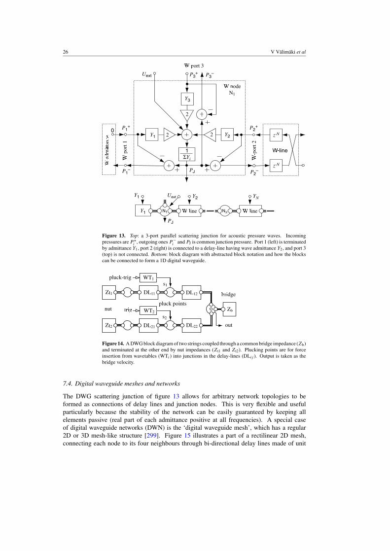
Figure 13 depicts the results of equations (41)–(44) as a signal flow diagram for thecomputation of an acoustic 3-port scattering junction. Due to the duality of variable pairs, thesame diagram can be applied to a series connection and volume velocity waves so that pressuresand volume velocities are interchanged and admittances are replaced by impedances.

In figure 13, port 1 is terminated by admittance Y1 and port 2 is connected to a delay-line ofadmittance Y2. Notice that for a passive termination Y1 the incoming port signal is zero so thatno computation is needed at that port. Port 3 is not connected. Dotted line regions show thegroupings of signal processing elements for block-based (object-based) computation, and thebottom part of the figure depicts an abstraction diagram of these blocks. Arbitrary admittancescan be given by their z-transforms as digital filters (FIR or IIR filters or just as real coefficientsif all attached impedances are real). Note that each admittance is also represented in the block1/

∑Yi . For real-valued admittances, the scattering junction computation can be optimized

to minimize the number of operations needed [253].An example of DWG string modelling in the mechanical domain is shown in figure 14,

where velocity waves are used and series connected junctions have equal velocity at eachport. A plucked string instrument with two strings is modelled by delay-line elements andtermination impedances Z = F/V , which are ratios of force F to velocity V . Plucking isinserted as force to a point in the string and the output is the vibration velocity at the bridge. Bothstrings have a common bridge impedance so that there is coupling between them. This leadsto ‘sympathetic vibrations’, whereby a vibrating string may transfer energy to another string,resulting in its vibration, too. For a full-scale model of the acoustic guitar, each string shouldhave two subsystems, one for vertical and another for horizontal vibration with a matrix-likecoupling of string polarities at the bridge, and six such string systems should be included.

26 V Valimaki et al

Y1

P1+

P1–

P3+ P3

–

ΣYi

Y3

ort 1

ort 3

odeN1

PJ

1

Y2 z-N

z-N

P2+

ort 2

P2–

Uext

0

ine

22

2

YN

ine

PJ

UextY1 Y2

N1 NNY1 ine

Figure 13. Top: a 3-port parallel scattering junction for acoustic pressure waves. Incomingpressures are P +

i , outgoing ones P −i and PJ is common junction pressure. Port 1 (left) is terminated

by admittance Y1, port 2 (right) is connected to a delay-line having wave admittance Y2, and port 3(top) is not connected. Bottom: block diagram with abstracted block notation and how the blockscan be connected to form a 1D digital waveguide.

Zt1

Zb

pluck points

pluck-trig

nut

out

dgeDL11 DL12

Zt2 DL21

WT1

WT2

DL22

s1

s2

Figure 14. A DWG block diagram of two strings coupled through a common bridge impedance (Zb)and terminated at the other end by nut impedances (Zt1 and Zt2). Plucking points are for forceinsertion from wavetables (WTi ) into junctions in the delay-lines (DLij ). Output is taken as thebridge velocity.

7.4. Digital waveguide meshes and networks

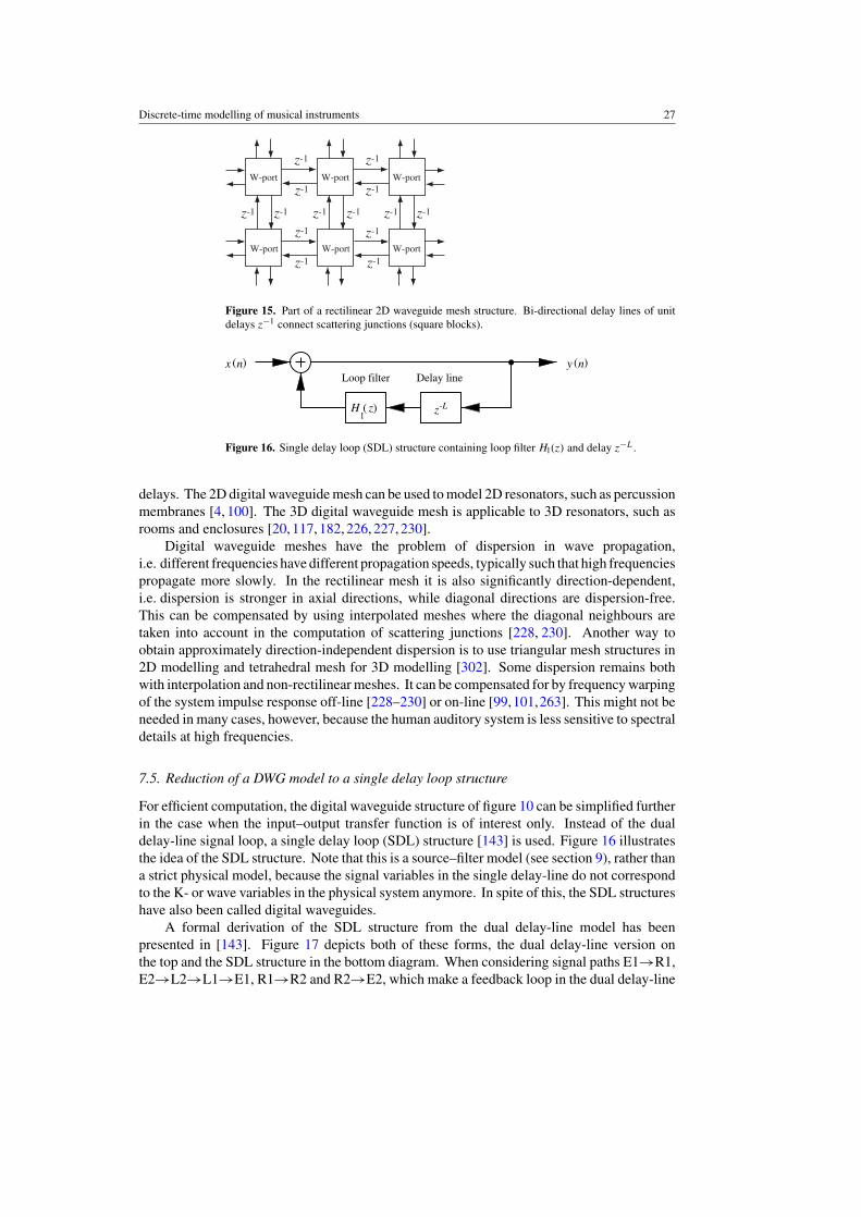
The DWG scattering junction of figure 13 allows for arbitrary network topologies to beformed as connections of delay lines and junction nodes. This is very flexible and usefulparticularly because the stability of the network can be easily guaranteed by keeping allelements passive (real part of each admittance positive at all frequencies). A special caseof digital waveguide networks (DWN) is the ‘digital waveguide mesh’, which has a regular2D or 3D mesh-like structure [299]. Figure 15 illustrates a part of a rectilinear 2D mesh,connecting each node to its four neighbours through bi-directional delay lines made of unit

Discrete-time modelling of musical instruments 27

z-1z-1z-1 z-1 z-1z-1

z-1

z-1

z-1

z-1

z-1 z-1

z-1z-1

W-port

W-portW-portW-port

W-portW-port

Figure 15. Part of a rectilinear 2D waveguide mesh structure. Bi-directional delay lines of unitdelays z−1 connect scattering junctions (square blocks).

H z( )l

-Lz

( )x nLoop filter Delay line

Figure 16. Single delay loop (SDL) structure containing loop filter Hl(z) and delay z−L.

delays. The 2D digital waveguide mesh can be used to model 2D resonators, such as percussionmembranes [4, 100]. The 3D digital waveguide mesh is applicable to 3D resonators, such asrooms and enclosures [20, 117, 182, 226, 227, 230].

Digital waveguide meshes have the problem of dispersion in wave propagation,i.e. different frequencies have different propagation speeds, typically such that high frequenciespropagate more slowly. In the rectilinear mesh it is also significantly direction-dependent,i.e. dispersion is stronger in axial directions, while diagonal directions are dispersion-free.This can be compensated by using interpolated meshes where the diagonal neighbours aretaken into account in the computation of scattering junctions [228, 230]. Another way toobtain approximately direction-independent dispersion is to use triangular mesh structures in2D modelling and tetrahedral mesh for 3D modelling [302]. Some dispersion remains bothwith interpolation and non-rectilinear meshes. It can be compensated for by frequency warpingof the system impulse response off-line [228–230] or on-line [99,101,263]. This might not beneeded in many cases, however, because the human auditory system is less sensitive to spectraldetails at high frequencies.

7.5. Reduction of a DWG model to a single delay loop structure

For efficient computation, the digital waveguide structure of figure 10 can be simplified furtherin the case when the input–output transfer function is of interest only. Instead of the dualdelay-line signal loop, a single delay loop (SDL) structure [143] is used. Figure 16 illustratesthe idea of the SDL structure. Note that this is a source–filter model (see section 9), rather thana strict physical model, because the signal variables in the single delay-line do not correspondto the K- or wave variables in the physical system anymore. In spite of this, the SDL structureshave also been called digital waveguides.

A formal derivation of the SDL structure from the dual delay-line model has beenpresented in [143]. Figure 17 depicts both of these forms, the dual delay-line version onthe top and the SDL structure in the bottom diagram. When considering signal paths E1→R1,E2→L2→L1→E1, R1→R2 and R2→E2, which make a feedback loop in the dual delay-line

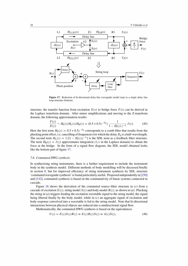
28 V Valimaki et al

Delay line

Delay line

–Hr(s)–Hl (s)Excitation

E1

E2L2

L1 R1

R2

X(s)

X(z)

X1(s)

X2(s)

Y1(s)

Y2(s)

1/2Rs

F(s)

F(z)

+

–

Bridgeforce

HE2,L2(s)

HL1,E1(s) HE,R(s)

⊕

-Integrator

DelayString loop

Pluck position

-+

+

LoopDelay filter

Figure 17. Reduction of bi-directional delay-line waveguide model (top) to a single delay lineloop structure (bottom).

structure, the transfer function from excitation X(s) to bridge force F(s) can be derived inthe Laplace transform domain. After minor simplifications and moving to the Z-transformdomain, the following approximation results:

F(z)

X(z)∼ HE(z)HL(z)HB(z) = (0.5 + 0.5z−Dp)

1

1 − Hl(z) z−LI (z). (45)

Here the first term HE(z) = 0.5 + 0.5z−Dp corresponds to a comb filter that results from theplucking point effect, i.e. cancelling of frequencies for which the delay Dp is a half-wavelength.The second term HL(z) = 1/[1 − Hl(z)z

−L] is the SDL term as a feedback filter structure.The term HB(z) = I (z) approximates integration (1/s in the Laplace domain) to obtain theforce at the bridge. In the form of a signal flow diagram, the SDL model obtained lookslike the bottom part of figure 17.

7.6. Commuted DWG synthesis

In synthesizing string instruments, there is a further requirement to include the instrumentbody in the synthesis model. Different methods of body modelling will be discussed brieflyin section 9, but for improved efficiency of string instrument synthesis by SDL structure‘commuted waveguide synthesis’ is found particularly useful. Proposed independently in [250]and [142], commuted synthesis is based on the commutativity of linear systems connected incascade.

Figure 18 shows the derivation of the commuted source–filter structure in (c) from acascade of excitation E(z), string model S(z) and body model B(z), as shown in (a). Pluckingthe string in (a) triggers feeding the excitation wavetable signal to the string model, the signalbeing filtered finally by the body model, while in (c) an aggregate signal of excitation andbody response convolved into a wavetable is fed to the string model. Note that bi-directionalinteractions between physical objects are reduced into a unidirectional signal flow.

Mathematically, the commuted DWG synthesis is based on the equivalences

Y (z) = E(z)S(z)B(z) ≡ E(z)B(z)S(z) ≡ A(z)S(z), (46)

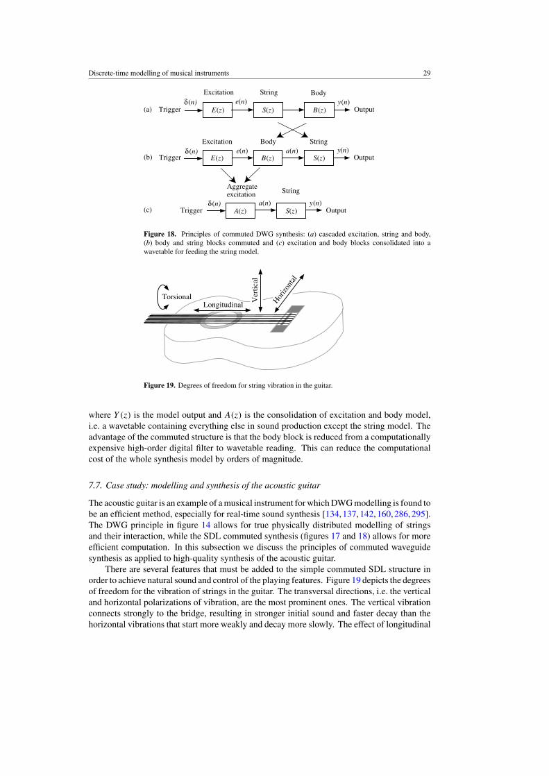
Discrete-time modelling of musical instruments 29

Excitationδ(n)

Body

OutputE(z)y(n)

Stringe(n)

B(z) S(z)Triggera(n)

Aggregateexcitation

δ(n)OutputA(z)

y(n)

String

a(n)S(z)Trigger

Excitationδ(n)

S(z)

Body

OutputE(z)y(n)

Stringe(n)

B(z)Trigger(a)

(b)

(c)

Figure 18. Principles of commuted DWG synthesis: (a) cascaded excitation, string and body,(b) body and string blocks commuted and (c) excitation and body blocks consolidated into awavetable for feeding the string model.

Longitudinal

Ver

tical

Hor

izon

tal

Torsional

Figure 19. Degrees of freedom for string vibration in the guitar.

where Y (z) is the model output and A(z) is the consolidation of excitation and body model,i.e. a wavetable containing everything else in sound production except the string model. Theadvantage of the commuted structure is that the body block is reduced from a computationallyexpensive high-order digital filter to wavetable reading. This can reduce the computationalcost of the whole synthesis model by orders of magnitude.

7.7. Case study: modelling and synthesis of the acoustic guitar

The acoustic guitar is an example of a musical instrument for which DWG modelling is found tobe an efficient method, especially for real-time sound synthesis [134,137,142,160,286,295].The DWG principle in figure 14 allows for true physically distributed modelling of stringsand their interaction, while the SDL commuted synthesis (figures 17 and 18) allows for moreefficient computation. In this subsection we discuss the principles of commuted waveguidesynthesis as applied to high-quality synthesis of the acoustic guitar.

There are several features that must be added to the simple commuted SDL structure inorder to achieve natural sound and control of the playing features. Figure 19 depicts the degreesof freedom for the vibration of strings in the guitar. The transversal directions, i.e. the verticaland horizontal polarizations of vibration, are the most prominent ones. The vertical vibrationconnects strongly to the bridge, resulting in stronger initial sound and faster decay than thehorizontal vibrations that start more weakly and decay more slowly. The effect of longitudinal

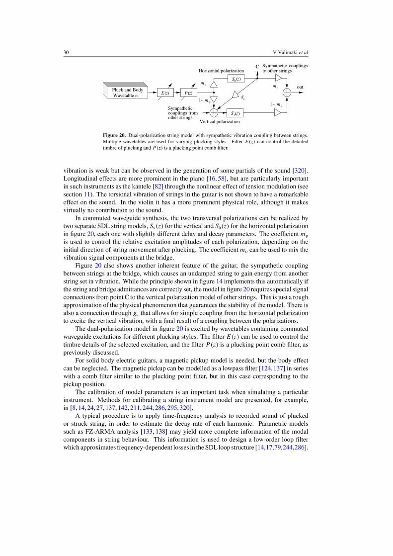
30 V Valimaki et al

v

h

Sympathetic

other strings

Horizontal polarization

Vertical polarization

C

out

( )

couplings from

S z

( )S z

m

m p1-om

om p

1-

( )Pluck and BodyWavetable n P z

gc

Sympathetic couplingsto other strings

E z( )

Figure 20. Dual-polarization string model with sympathetic vibration coupling between strings.Multiple wavetables are used for varying plucking styles. Filter E(z) can control the detailedtimbre of plucking and P(z) is a plucking point comb filter.

vibration is weak but can be observed in the generation of some partials of the sound [320].Longitudinal effects are more prominent in the piano [16, 58], but are particularly importantin such instruments as the kantele [82] through the nonlinear effect of tension modulation (seesection 11). The torsional vibration of strings in the guitar is not shown to have a remarkableeffect on the sound. In the violin it has a more prominent physical role, although it makesvirtually no contribution to the sound.

In commuted waveguide synthesis, the two transversal polarizations can be realized bytwo separate SDL string models, Sv(z) for the vertical and Sh(z) for the horizontal polarizationin figure 20, each one with slightly different delay and decay parameters. The coefficient mp

is used to control the relative excitation amplitudes of each polarization, depending on theinitial direction of string movement after plucking. The coefficient mo can be used to mix thevibration signal components at the bridge.

Figure 20 also shows another inherent feature of the guitar, the sympathetic couplingbetween strings at the bridge, which causes an undamped string to gain energy from anotherstring set in vibration. While the principle shown in figure 14 implements this automatically ifthe string and bridge admittances are correctly set, the model in figure 20 requires special signalconnections from point C to the vertical polarization model of other strings. This is just a roughapproximation of the physical phenomenon that guarantees the stability of the model. There isalso a connection through gc that allows for simple coupling from the horizontal polarizationto excite the vertical vibration, with a final result of a coupling between the polarizations.

The dual-polarization model in figure 20 is excited by wavetables containing commutedwaveguide excitations for different plucking styles. The filter E(z) can be used to control thetimbre details of the selected excitation, and the filter P(z) is a plucking point comb filter, aspreviously discussed.

For solid body electric guitars, a magnetic pickup model is needed, but the body effectcan be neglected. The magnetic pickup can be modelled as a lowpass filter [124,137] in serieswith a comb filter similar to the plucking point filter, but in this case corresponding to thepickup position.

The calibration of model parameters is an important task when simulating a particularinstrument. Methods for calibrating a string instrument model are presented, for example,in [8, 14, 24, 27, 137, 142, 211, 244, 286, 295, 320].

A typical procedure is to apply time-frequency analysis to recorded sound of pluckedor struck string, in order to estimate the decay rate of each harmonic. Parametric modelssuch as FZ-ARMA analysis [133, 138] may yield more complete information of the modalcomponents in string behaviour. This information is used to design a low-order loop filterwhich approximates frequency-dependent losses in the SDL loop structure [14,17,79,244,286].

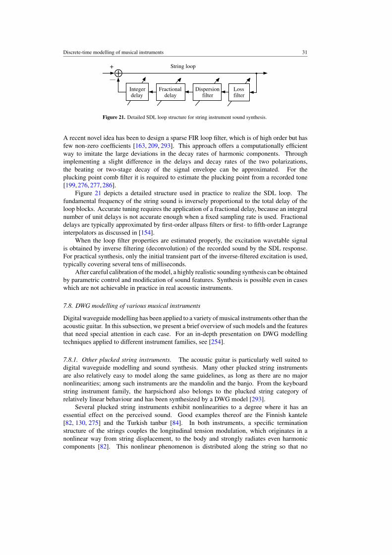
Discrete-time modelling of musical instruments 31

—

String loop+⊕

Integerdelay

Fractionaldelay

Dispersionfilter

Lossfilter

Figure 21. Detailed SDL loop structure for string instrument sound synthesis.

A recent novel idea has been to design a sparse FIR loop filter, which is of high order but hasfew non-zero coefficients [163, 209, 293]. This approach offers a computationally efficientway to imitate the large deviations in the decay rates of harmonic components. Throughimplementing a slight difference in the delays and decay rates of the two polarizations,the beating or two-stage decay of the signal envelope can be approximated. For theplucking point comb filter it is required to estimate the plucking point from a recorded tone[199, 276, 277, 286].

Figure 21 depicts a detailed structure used in practice to realize the SDL loop. Thefundamental frequency of the string sound is inversely proportional to the total delay of theloop blocks. Accurate tuning requires the application of a fractional delay, because an integralnumber of unit delays is not accurate enough when a fixed sampling rate is used. Fractionaldelays are typically approximated by first-order allpass filters or first- to fifth-order Lagrangeinterpolators as discussed in [154].

When the loop filter properties are estimated properly, the excitation wavetable signalis obtained by inverse filtering (deconvolution) of the recorded sound by the SDL response.For practical synthesis, only the initial transient part of the inverse-filtered excitation is used,typically covering several tens of milliseconds.

After careful calibration of the model, a highly realistic sounding synthesis can be obtainedby parametric control and modification of sound features. Synthesis is possible even in caseswhich are not achievable in practice in real acoustic instruments.

7.8. DWG modelling of various musical instruments

Digital waveguide modelling has been applied to a variety of musical instruments other than theacoustic guitar. In this subsection, we present a brief overview of such models and the featuresthat need special attention in each case. For an in-depth presentation on DWG modellingtechniques applied to different instrument families, see [254].

7.8.1. Other plucked string instruments. The acoustic guitar is particularly well suited todigital waveguide modelling and sound synthesis. Many other plucked string instrumentsare also relatively easy to model along the same guidelines, as long as there are no majornonlinearities; among such instruments are the mandolin and the banjo. From the keyboardstring instrument family, the harpsichord also belongs to the plucked string category ofrelatively linear behaviour and has been synthesized by a DWG model [293].

Several plucked string instruments exhibit nonlinearities to a degree where it has anessential effect on the perceived sound. Good examples thereof are the Finnish kantele[82, 130, 275] and the Turkish tanbur [84]. In both instruments, a specific terminationstructure of the strings couples the longitudinal tension modulation, which originates in anonlinear way from string displacement, to the body and strongly radiates even harmoniccomponents [82]. This nonlinear phenomenon is distributed along the string so that no

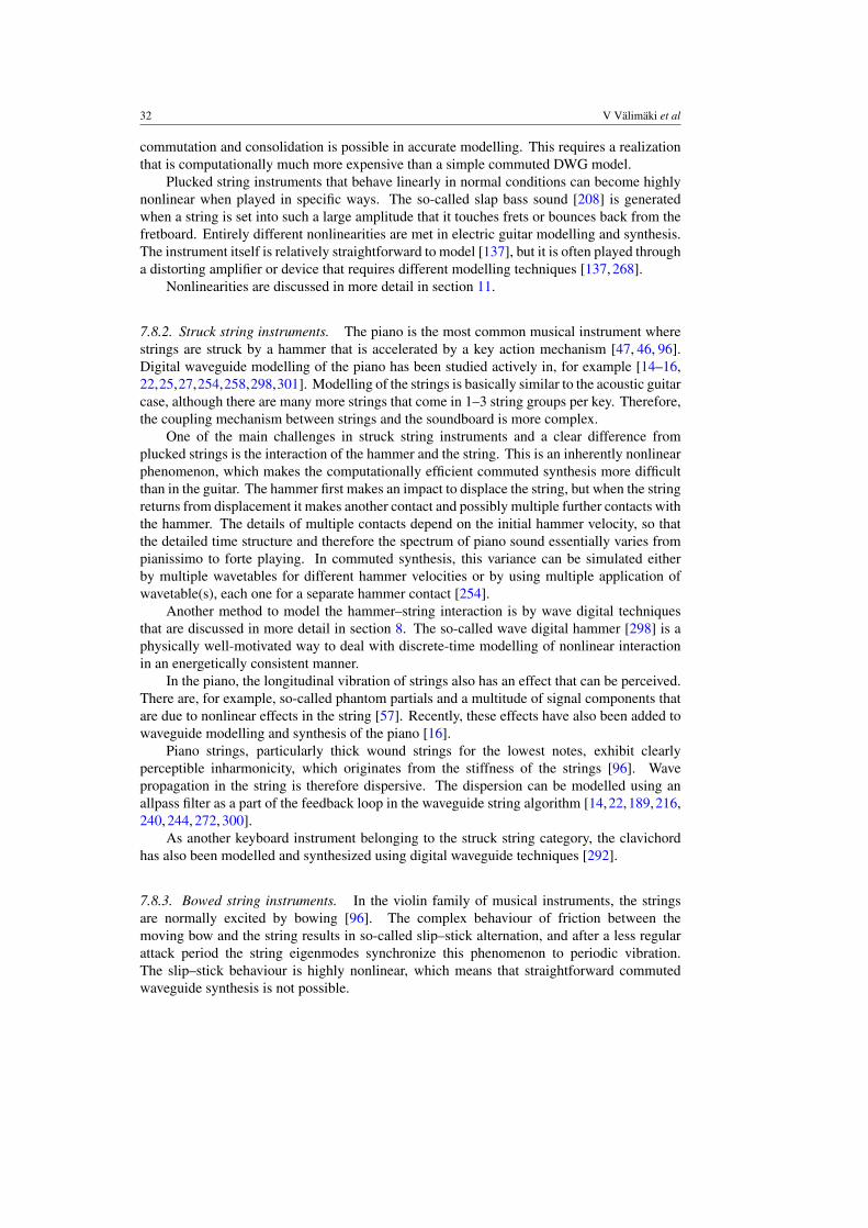
32 V Valimaki et al

commutation and consolidation is possible in accurate modelling. This requires a realizationthat is computationally much more expensive than a simple commuted DWG model.

Plucked string instruments that behave linearly in normal conditions can become highlynonlinear when played in specific ways. The so-called slap bass sound [208] is generatedwhen a string is set into such a large amplitude that it touches frets or bounces back from thefretboard. Entirely different nonlinearities are met in electric guitar modelling and synthesis.The instrument itself is relatively straightforward to model [137], but it is often played througha distorting amplifier or device that requires different modelling techniques [137, 268].

Nonlinearities are discussed in more detail in section 11.

7.8.2. Struck string instruments. The piano is the most common musical instrument wherestrings are struck by a hammer that is accelerated by a key action mechanism [47, 46, 96].Digital waveguide modelling of the piano has been studied actively in, for example [14–16,22,25,27,254,258,298,301]. Modelling of the strings is basically similar to the acoustic guitarcase, although there are many more strings that come in 1–3 string groups per key. Therefore,the coupling mechanism between strings and the soundboard is more complex.

One of the main challenges in struck string instruments and a clear difference fromplucked strings is the interaction of the hammer and the string. This is an inherently nonlinearphenomenon, which makes the computationally efficient commuted synthesis more difficultthan in the guitar. The hammer first makes an impact to displace the string, but when the stringreturns from displacement it makes another contact and possibly multiple further contacts withthe hammer. The details of multiple contacts depend on the initial hammer velocity, so thatthe detailed time structure and therefore the spectrum of piano sound essentially varies frompianissimo to forte playing. In commuted synthesis, this variance can be simulated eitherby multiple wavetables for different hammer velocities or by using multiple application ofwavetable(s), each one for a separate hammer contact [254].

Another method to model the hammer–string interaction is by wave digital techniquesthat are discussed in more detail in section 8. The so-called wave digital hammer [298] is aphysically well-motivated way to deal with discrete-time modelling of nonlinear interactionin an energetically consistent manner.

In the piano, the longitudinal vibration of strings also has an effect that can be perceived.There are, for example, so-called phantom partials and a multitude of signal components thatare due to nonlinear effects in the string [57]. Recently, these effects have also been added towaveguide modelling and synthesis of the piano [16].

Piano strings, particularly thick wound strings for the lowest notes, exhibit clearlyperceptible inharmonicity, which originates from the stiffness of the strings [96]. Wavepropagation in the string is therefore dispersive. The dispersion can be modelled using anallpass filter as a part of the feedback loop in the waveguide string algorithm [14,22,189,216,240, 244, 272, 300].

As another keyboard instrument belonging to the struck string category, the clavichordhas also been modelled and synthesized using digital waveguide techniques [292].

7.8.3. Bowed string instruments. In the violin family of musical instruments, the stringsare normally excited by bowing [96]. The complex behaviour of friction between themoving bow and the string results in so-called slip–stick alternation, and after a less regularattack period the string eigenmodes synchronize this phenomenon to periodic vibration.The slip–stick behaviour is highly nonlinear, which means that straightforward commutedwaveguide synthesis is not possible.

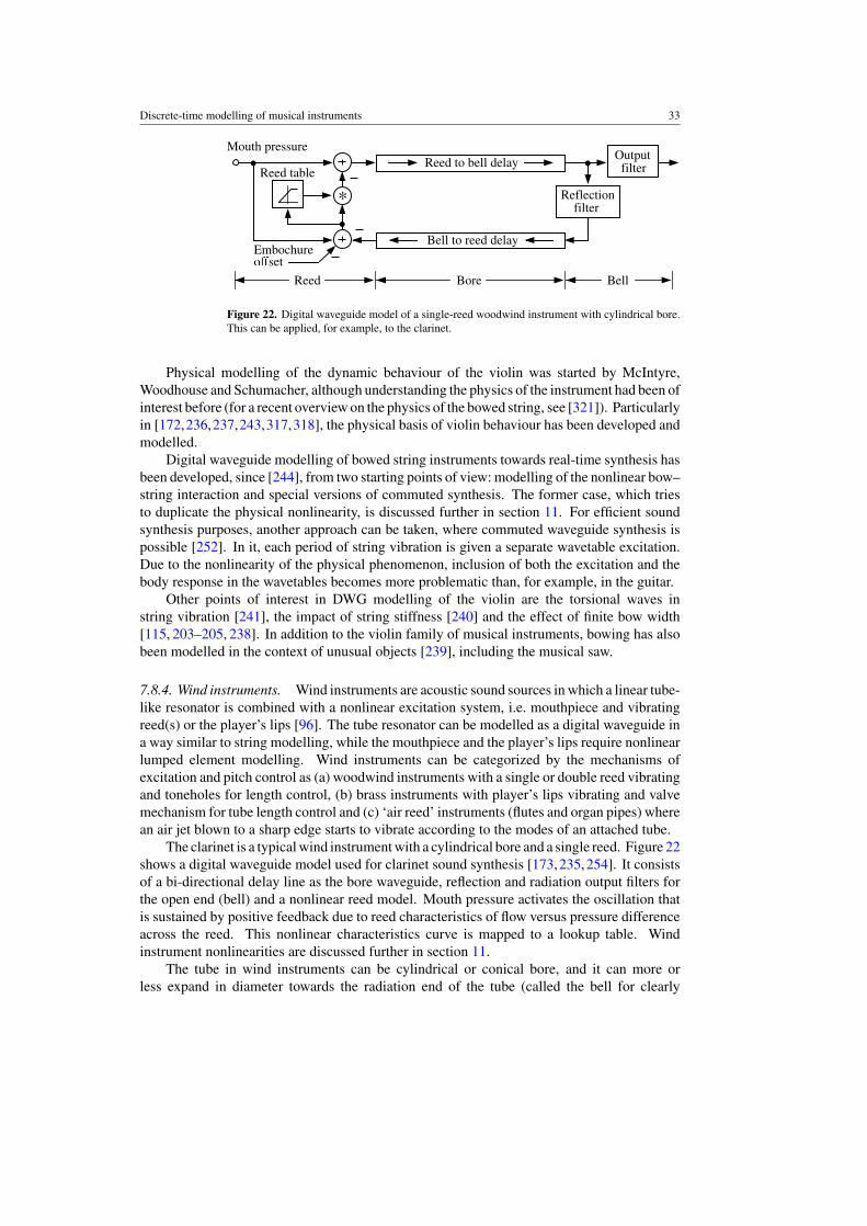
Discrete-time modelling of musical instruments 33

Reed to bell delayMouth pressure

Reed table

Embochureset

Reflection filter

Output filter

Bell to reed delay

Bore BellReed

*

Figure 22. Digital waveguide model of a single-reed woodwind instrument with cylindrical bore.This can be applied, for example, to the clarinet.

Physical modelling of the dynamic behaviour of the violin was started by McIntyre,Woodhouse and Schumacher, although understanding the physics of the instrument had been ofinterest before (for a recent overview on the physics of the bowed string, see [321]). Particularlyin [172,236,237,243,317,318], the physical basis of violin behaviour has been developed andmodelled.

Digital waveguide modelling of bowed string instruments towards real-time synthesis hasbeen developed, since [244], from two starting points of view: modelling of the nonlinear bow–string interaction and special versions of commuted synthesis. The former case, which triesto duplicate the physical nonlinearity, is discussed further in section 11. For efficient soundsynthesis purposes, another approach can be taken, where commuted waveguide synthesis ispossible [252]. In it, each period of string vibration is given a separate wavetable excitation.Due to the nonlinearity of the physical phenomenon, inclusion of both the excitation and thebody response in the wavetables becomes more problematic than, for example, in the guitar.

Other points of interest in DWG modelling of the violin are the torsional waves instring vibration [241], the impact of string stiffness [240] and the effect of finite bow width[115, 203–205, 238]. In addition to the violin family of musical instruments, bowing has alsobeen modelled in the context of unusual objects [239], including the musical saw.

7.8.4. Wind instruments. Wind instruments are acoustic sound sources in which a linear tube-like resonator is combined with a nonlinear excitation system, i.e. mouthpiece and vibratingreed(s) or the player’s lips [96]. The tube resonator can be modelled as a digital waveguide ina way similar to string modelling, while the mouthpiece and the player’s lips require nonlinearlumped element modelling. Wind instruments can be categorized by the mechanisms ofexcitation and pitch control as (a) woodwind instruments with a single or double reed vibratingand toneholes for length control, (b) brass instruments with player’s lips vibrating and valvemechanism for tube length control and (c) ‘air reed’ instruments (flutes and organ pipes) wherean air jet blown to a sharp edge starts to vibrate according to the modes of an attached tube.

The clarinet is a typical wind instrument with a cylindrical bore and a single reed. Figure 22shows a digital waveguide model used for clarinet sound synthesis [173,235,254]. It consistsof a bi-directional delay line as the bore waveguide, reflection and radiation output filters forthe open end (bell) and a nonlinear reed model. Mouth pressure activates the oscillation thatis sustained by positive feedback due to reed characteristics of flow versus pressure differenceacross the reed. This nonlinear characteristics curve is mapped to a lookup table. Windinstrument nonlinearities are discussed further in section 11.

The tube in wind instruments can be cylindrical or conical bore, and it can more orless expand in diameter towards the radiation end of the tube (called the bell for clearly

34 V Valimaki et al

expanding cases). Modelling of the instrument bores has been studied in [19, 61, 70, 77, 231,246, 248, 283, 287, 303, 304, 306, 307]. Conical and exponentially expanding bores are moredemanding to simulate than the cylindrical ones [19, 70, 77, 231, 248, 267, 283, 287, 303, 304,306, 307].

Another part of wind instruments that requires modelling effort are the toneholes, whichare controllable side branch openings in the waveguide. Tonehole modelling is studied, forexample, in [28, 231, 232, 283, 290, 305]. When open, a tonehole works similarly to an openend, and the rest of the bore towards the bell has little effect on sound production. When atonehole is closed, it corresponds to a short closed tube that has a minor effect on the wavepassing it.

Examples of brass instrument modelling are found, for example, in [312,313]. Modellingof the player’s lip vibration is similar to the case of vocal fold modelling in speech and singing,and it can be realized as a self-oscillating nonlinearity.

Yet another phenomenon of interest in brass instruments is the high pressure level of wavesin the instrument bore, which exhibits slight nonlinearity in air compression, and results inthe formation of shock waves [180, 181, 314]. This has to be taken into account in detailedmodelling of loud sounds with their particular ‘metallic’ timbre, for example, in the trumpetand the trombone.

The flute and its air jet oscillation have been modelled by digital waveguide principlesin [288, 309].

7.8.5. Percussion instruments. Percussive instruments, such as drums and gongs, have beenstudied from a physical point of view and with numerical methods, for example, in [49, 51,52, 210], and they have been modelled and synthesized using 2D digital waveguide meshesin [299,300]. (Actually those resonators are 3D objects if the air loading is taken into account.)For 2D (and 3D) digital waveguides there is no way to consolidate the structure of figure 15as can be done in the 1D case (see figure 9). Therefore, the wave-based computation of digitalwaveguide meshes can become expensive for large structures. The losses can be commutedto waveguide terminations, which allows the mesh itself to be lossless and thus maximallysimple.

Although the waveguide meshes are dispersive and therefore the higher modes do not havecorrect frequencies, it is acceptable due to the reduced frequency resolution of human auditoryperception at high frequencies.

Many 2D resonators in percussive instruments exhibit nonlinear behaviour. This isparticularly true for gong-like instruments [96]. Such nonlinearities make strong inter-modecoupling so that the vibration energy can spread, for example, from low to high frequencieswith audible shift in timbre. The nonlinearities themselves are inherently lossless and requirespecial techniques for simulation. Methods to realize such passive nonlinearities were proposedin [202,296] and are briefly discussed in section 11. In a waveguide mesh synthesis of a gong,it may suffice to add passive nonlinearities only at the rim termination of the instrumentmodel mesh, although in a real gong they are distributed. A further step in modellingcomplexity from gongs is the Caribbean steel pan (steel drum) [96], where the distributionof modal patterns creates regions tuned to different pitches and the nonlinearities make a richtimbre.

7.8.6. Speech and singing voice. As mentioned above, modelling of voice production wasthe early application of digital waveguide principle, at that time called the transmission lineprinciple [145]. Since then, the same principle has been used in numerous simulations of

Discrete-time modelling of musical instruments 35

speech production, see for example [59, 128, 164, 267, 289], and in singing voice synthesis[59, 60, 64, 150, 151], although it has not become popular in practical speech synthesis,partly due to computational complexity compared with formant synthesis (see section 9) andconcatenation methods based on samples from real speech.

In voice production, the DWG principle can be applied to the vocal (and nasal) tract bysplicing it to short sections from the glottis to the lips. The admittance of each section iscontrolled proportionally to the cross-sectional area in that position. The method is well suitedto articulatory modelling and synthesis whereby the movements of the articulators, particularlyof the tongue, can be mapped to the area profile for vocal tract control.

7.8.7. Inharmonic SDL type of DWG models. Digital waveguides are most straightforwardand efficient when applied to instruments producing harmonic spectrum of sound; this iswhat a simple terminated delay line does when excited. The majority of instruments used inwestern music produce fully or approximately harmonic sounds. DWGs needed for stronglyinharmonic sounds are necessarily more complex.

An example on DWG modelling of highly inharmonic instruments is synthesis of bellsounds [140, 141]. By including a highly dispersive second-order allpass filter within a SDLfeedback loop it was found that bell sounds can be synthesized by an efficient DWG model.Although only the lowest partials can be tuned relatively accurately, the perceptual quality ofDWG bell models can be made close to real bells. Notice that in this case the model does notanyhow correspond to the spatial geometric structure and vibration distribution of a real bell.Rather, this is a generic DWG model tuned in its parameters to produce realistic bell sounds.

8. Wave digital filters

The purpose of this section is to provide a general overview of physical modelling using WDFsin the context of musical instruments. Only the essential basics of the topic will be discussedin detail; the rest will be glossed over. For more information about the subject, the reader isencouraged to refer to [254]. Also, another definitive work can be found in [94].

8.1. What are wave digital filters?

WDFs were developed in the late 1960s by Alfred Fettweis [93] for digitizing lumped analogelectrical circuits. The travelling-wave formulation of lumped electrical elements, where theWDF approach is based, was introduced earlier by Belevitch [21, 254].

WDFs are certain types of digital filters with valid interpretations in the physical world.This means that we can simulate the behaviour of a lumped physical system using a digitalfilter whose coefficients depend on the parameters of this physical system. Alternatively,WDFs can be seen as a particular type of finite difference scheme with excellent numericalproperties [254]. As discussed in section 4, the task of finite difference schemes in general is toprovide discrete versions of partial differential equations for simulation and analysis purposes.

WDFs are useful for physical modelling in many respects. Firstly, they are modular: thesame building blocks can be used for modelling very different systems; all that needs to bechanged is the topology of the wave digital network. Secondly, the preservation of energy andhence also stability is usually addressed, since the elementary blocks can be made passive,and the energy preservation between blocks are evaluated using the Kirchhoff’s laws. Finally,WDFs have good numerical properties, that is, they do not experience artificial damping athigh frequencies.

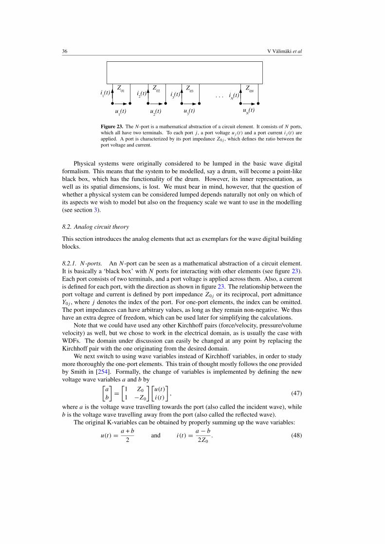
36 V Valimaki et al

Figure 23. The N -port is a mathematical abstraction of a circuit element. It consists of N ports,which all have two terminals. To each port j , a port voltage uj (t) and a port current ij (t) areapplied. A port is characterized by its port impedance Z0j , which defines the ratio between theport voltage and current.

Physical systems were originally considered to be lumped in the basic wave digitalformalism. This means that the system to be modelled, say a drum, will become a point-likeblack box, which has the functionality of the drum. However, its inner representation, aswell as its spatial dimensions, is lost. We must bear in mind, however, that the question ofwhether a physical system can be considered lumped depends naturally not only on which ofits aspects we wish to model but also on the frequency scale we want to use in the modelling(see section 3).

8.2. Analog circuit theory

This section introduces the analog elements that act as exemplars for the wave digital buildingblocks.

8.2.1. N -ports. An N -port can be seen as a mathematical abstraction of a circuit element.It is basically a ‘black box’ with N ports for interacting with other elements (see figure 23).Each port consists of two terminals, and a port voltage is applied across them. Also, a currentis defined for each port, with the direction as shown in figure 23. The relationship between theport voltage and current is defined by port impedance Z0j or its reciprocal, port admittanceY0j , where j denotes the index of the port. For one-port elements, the index can be omitted.The port impedances can have arbitrary values, as long as they remain non-negative. We thushave an extra degree of freedom, which can be used later for simplifying the calculations.

Note that we could have used any other Kirchhoff pairs (force/velocity, pressure/volumevelocity) as well, but we chose to work in the electrical domain, as is usually the case withWDFs. The domain under discussion can easily be changed at any point by replacing theKirchhoff pair with the one originating from the desired domain.

We next switch to using wave variables instead of Kirchhoff variables, in order to studymore thoroughly the one-port elements. This train of thought mostly follows the one providedby Smith in [254]. Formally, the change of variables is implemented by defining the newvoltage wave variables a and b by[

a

b

]=

[1 Z0

1 −Z0

] [u(t)

i(t)

], (47)

where a is the voltage wave travelling towards the port (also called the incident wave), whileb is the voltage wave travelling away from the port (also called the reflected wave).

The original K-variables can be obtained by properly summing up the wave variables:

u(t) = a + b

2and i(t) = a − b

2Z0. (48)

Discrete-time modelling of musical instruments 37

It is worth noting that this differs from the wave decomposition often done in digital waveguides(see, e.g. [253]), where the K-variables are obtained by summing the wave variables withoutthe scaling-by-two. We will discuss this in more detail in section 8.5.4.

Reflectance of a port is the transfer function that indicates the relation between an incomingand an outgoing wave to that port. Formally, it can be obtained from the Laplace transform ofthe reflected wave, divided by the Laplace transform of the incoming wave [254]:

SZ(s) = L{b}L{a} = L{u(t) − Z0i(t)}

L{u(t) + Z0i(t)} = Z(s) − Z0

Z(s) + Z0, (49)

where L is the Laplace operator. Note that here we used voltage waves in defining thereflectance; had we used current waves, we would have obtained another formulation forthe reflectance. Therefore, this result can also be called the voltage-wave reflectance or theforce-wave reflectance in the mechanical domain.

8.2.2. One-port elements. This section will discuss the basic one-port elements: capacitors,inductors, resistors, open- and short-circuits and voltage and current sources. We will derivetheir individual reflectances in a similar way as in [254]. Two-port elements, such as gyrators,transformers and QUARLs, are discussed, e.g. in [94].

For a capacitor, it holds that the current i(t) flowing through the element is proportionalto the time derivative of the voltage u(t) across it:

i(t) = C∂u(t)

∂t, (50)

where C is the capacitance in Farads. Using the Laplace transform, we have

I (s) = CsU(s), (51)

where s is the complex frequency variable, and I (s) and U(s) stand for the current andvoltage in the complex frequency domain, respectively. Using the generalized Ohm’s law, theimpedance of a capacitor can now be given as

ZC(s) = 1

Cs. (52)

Substituting ZC(s) for Z(s) in equation (49), we obtain the reflectance of the capacitor as

SC(s) = ZC(s) − Z0

ZC(s) + Z0= 1 − Z0Cs

1 + Z0Cs. (53)

For an inductor, the voltage is in turn proportional to the time derivative of the current:

v(t) = L∂i(t)

∂t, (54)

where L denotes the inductance in Henrys. Similarly, taking the Laplace transform andcalculating the impedance, we have

ZL(s) = Ls. (55)

Substituting this result into equation (49), we obtain the reflectance of the inductor as

SL(s) = ZL(s) − Z0

ZL(s) + Z0= s − Z0/L

s + Z0/L. (56)

For a resistor, we have

u(t) = Ri(t), (57)

38 V Valimaki et al

where R is the resistance (in Ohms), and for the impedance we get simply

ZR(s) = R. (58)

Thus, the reflectance of the resistor becomes

SR(s) = 1 − Z0/R

1 + Z0/R. (59)

Obviously, for the open and short circuit impedances, we have

Zoc(s) = ∞ (60)

and

Zsc(s) = 0, (61)

respectively. Hence, the reflectances become

Soc(s) = 1 (62)

and

Ssc(s) = −1. (63)

Note that this corroborates with our knowledge of wave propagation. An open circuit reflectsvoltage waves without changing their phase, whereas the short circuit inverts the phase of thereflecting voltage. In mechanical terms, a rigid wall termination reflects force waves withoutphase inversion, while a free ‘frictionless’ termination inverts the phase of the reflecting force.For velocity waves, such as the ones observable in a vibrating string4, the opposite is true: rigidterminations invert the phase, whereas free terminations preserve it.

We will consider voltage and current sources in their digitized form in section 8.3.3. Theseelements are needed if energy needs to be inserted into the system during run time. Otherwise,initializing the voltage and current of the circuit is sufficient.

8.3. Wave digital building blocks

This section discusses the digitized versions of the analog elements already introduced andprovides rules for connecting them to form networks.

8.3.1. Discretization using the bilinear transform. The discretization of the network elementsdiscussed in section 8.3.3 is implemented using the well-known bilinear transform:

s → ψ = 2

T

1 − z−1

1 + z−1= 2

Ttanh(sT /2), (64)

where z = esT denotes the discrete complex frequency, while T stands for the samplinginterval. By studying the real-valued discrete frequencies, we note that

Re[ψ] > 0 ⇔ Re

[2

T

esT − 1

esT + 1

]> 0 ⇔ Re[s] > 0 ⇔ |z| > 1, (65)

Re[ψ] < 0 ⇔ Re

[2

T

esT − 1

esT + 1

]< 0 ⇔ Re[s] < 0 ⇔ |z| < 1 (66)

and

Re[ψ] = 0 ⇔ Re

[2

T

esT − 1

esT + 1

]= 0 ⇔ Re[s] = 0 ⇔ |z| = 1. (67)

4 Actually, looking at a vibrating string one observes the displacement waves, but comparing them to their timederivative, i.e. the velocity waves, one notices that they reflect similarly.

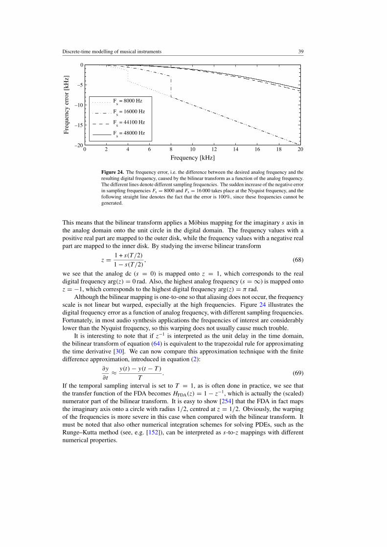
Discrete-time modelling of musical instruments 39

0 2 4 6 8 10 12 14 16 18 20–20

–15

–10

–5

0

Frequency [kHz]

Freq

uenc

y er

ror

[kH

z]

Fs = 8000 Hz

Fs = 16000 Hz

Fs = 44100 Hz

Fs = 48000 Hz

Figure 24. The frequency error, i.e. the difference between the desired analog frequency and theresulting digital frequency, caused by the bilinear transform as a function of the analog frequency.The different lines denote different sampling frequencies. The sudden increase of the negative errorin sampling frequencies Fs = 8000 and Fs = 16 000 takes place at the Nyquist frequency, and thefollowing straight line denotes the fact that the error is 100%, since these frequencies cannot begenerated.

This means that the bilinear transform applies a Mobius mapping for the imaginary s axis inthe analog domain onto the unit circle in the digital domain. The frequency values with apositive real part are mapped to the outer disk, while the frequency values with a negative realpart are mapped to the inner disk. By studying the inverse bilinear transform

z = 1 + s(T /2)

1 − s(T /2), (68)

we see that the analog dc (s = 0) is mapped onto z = 1, which corresponds to the realdigital frequency arg(z) = 0 rad. Also, the highest analog frequency (s = ∞) is mapped ontoz = −1, which corresponds to the highest digital frequency arg(z) = π rad.

Although the bilinear mapping is one-to-one so that aliasing does not occur, the frequencyscale is not linear but warped, especially at the high frequencies. Figure 24 illustrates thedigital frequency error as a function of analog frequency, with different sampling frequencies.Fortunately, in most audio synthesis applications the frequencies of interest are considerablylower than the Nyquist frequency, so this warping does not usually cause much trouble.

It is interesting to note that if z−1 is interpreted as the unit delay in the time domain,the bilinear transform of equation (64) is equivalent to the trapezoidal rule for approximatingthe time derivative [30]. We can now compare this approximation technique with the finitedifference approximation, introduced in equation (2):

∂y

∂t≈ y(t) − y(t − T )

T. (69)

If the temporal sampling interval is set to T = 1, as is often done in practice, we see thatthe transfer function of the FDA becomes HFDA(z) = 1 − z−1, which is actually the (scaled)numerator part of the bilinear transform. It is easy to show [254] that the FDA in fact mapsthe imaginary axis onto a circle with radius 1/2, centred at z = 1/2. Obviously, the warpingof the frequencies is more severe in this case when compared with the bilinear transform. Itmust be noted that also other numerical integration schemes for solving PDEs, such as theRunge–Kutta method (see, e.g. [152]), can be interpreted as s-to-z mappings with differentnumerical properties.

40 V Valimaki et al

8.3.2. Realizability. If the inductor element is now discretized using the bilinear transform,using equation (56), its reflectance becomes

SL

(2

T

1 − z−1

1 + z−1

)= (2/T − Z0/L) − (Z0/L + 2/T )z−1

(2/T + Z0/L) + (Z0/L − 2/T )z−1. (70)

Now, remembering that reflectance is actually the transfer function from the incident wave tothe reflected one, we see that it has a delay-free term in the nominator. When this element isconnected into a junction, we see that the incident wave (looking from the element’s view) isevaluated using the reflected wave. Now, since there is a delay-free term in the reflectance ofthis element, the system becomes implicit, since we would need the instantaneous output ofthe system when calculating the input. Fortunately, we can solve this problem by utilizing theextra degree of freedom, the port impedance, by assigning an appropriate value for it.

8.3.3. One-port elements. Defining Z0 = ZL = 2L/T for the impedance of the wave digitalinductor in equation (56), the reflectance simplifies to

SL(z) = −z−1. (71)

Similarly, selecting Z0 = ZC = T/(2C) for the impedance of the wave digital capacitor inequation (53) simplifies reflectance to

SC(z) = z−1. (72)

Since the reflectance of the resistor is memoryless, i.e. there is no s-term in equation (59),we can simply choose Z0 = ZR = R for the resistor’s impedance in equation (59), and thereflectance goes to zero:

SR(z) = 0, (73)

which means that there is no reflection from the one-port resistor element. We will later findout how connecting a wave digital resistor can still affect a system.

Voltage and current sources can also be implemented as wave digital elements. For thevoltage source, we have [94]

Su(z) = 2e − 1, (74)

and for the current source

Si(z) = 1 − 2e, (75)

where e is the voltage generated by the source. Table 1 summarizes the one-port elementsdiscussed thus far.

8.4. Interconnection and adaptors

The interconnection of different one-port elements is possible using adaptors. Adaptorsare N -port interfaces that enable the connection of other N -port elements and implementthe wave scattering resulting from the different port impedances. There are two types ofadaptors: parallel and series. The parallel adaptor is the wave digital equivalent of theparallel connection from basic circuit theory. N -port elements connected in parallel share thesame voltage, while their currents sum up to zero. Intuitively, the series adaptor is in turnthe wave digital equivalent of the series connection. N -port elements connected in series sharethe current and the voltages sum up to zero.

In this section, we will derive the scattering rules first for two-port parallel and seriesadaptors, after which we will extend these results for obtaining the scattering rules forN -port adaptors. This derivation process follows the guidelines presented in the WDFliterature [94, 254].

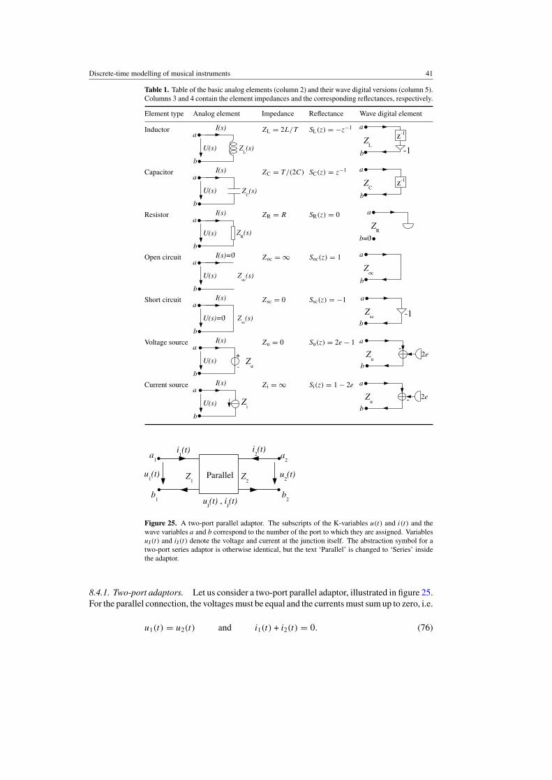
Discrete-time modelling of musical instruments 41

Table 1. Table of the basic analog elements (column 2) and their wave digital versions (column 5).Columns 3 and 4 contain the element impedances and the corresponding reflectances, respectively.

Element type Analog element Impedance Reflectance Wave digital element

Inductor ZL = 2L/T SL(z) = −z−1

Capacitor ZC = T/(2C) SC(z) = z−1

Resistor ZR = R SR(z) = 0

Open circuit Zoc = ∞ Soc(z) = 1

Short circuit Zsc = 0 Ssc(z) = −1

Voltage source Zu = 0 Su(z) = 2e − 1

Current source Zi = ∞ Si(z) = 1 − 2e

Figure 25. A two-port parallel adaptor. The subscripts of the K-variables u(t) and i(t) and thewave variables a and b correspond to the number of the port to which they are assigned. VariablesuJ(t) and iJ(t) denote the voltage and current at the junction itself. The abstraction symbol for atwo-port series adaptor is otherwise identical, but the text ‘Parallel’ is changed to ‘Series’ insidethe adaptor.

8.4.1. Two-port adaptors. Let us consider a two-port parallel adaptor, illustrated in figure 25.For the parallel connection, the voltages must be equal and the currents must sum up to zero, i.e.

u1(t) = u2(t) and i1(t) + i2(t) = 0. (76)

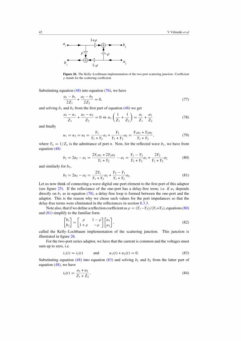
42 V Valimaki et al

Figure 26. The Kelly–Lochbaum implementation of the two-port scattering junction. Coefficientρ stands for the scattering coefficient.

Substituting equation (48) into equation (76), we have

a1 − b1

2Z1+

a2 − b2

2Z2= 0, (77)

and solving b1 and b2 from the first part of equation (48) we get

a1 − u1

Z1+

a2 − u2

Z2= 0 ⇔ u1

(1

Z1+

1

Z2

)= a1

Z1+

a2

Z2(78)

and finally

u1 = u2 = uJ = Y1

Y1 + Y2a1 +

Y2

Y1 + Y2a2 = Y1a1 + Y2a2

Y1 + Y2, (79)

where Yn = 1/Zn is the admittance of port n. Now, for the reflected wave b1, we have fromequation (48)

b1 = 2uJ − a1 = 2Y1a1 + 2Y2a2

Y1 + Y2− a1 = Y1 − Y2

Y1 + Y2a1 +

2Y2

Y1 + Y2a2 (80)

and similarly for b2,

b2 = 2uJ − a2 = 2Y1

Y1 + Y2a1 +

Y2 − Y1

Y1 + Y2a2. (81)

Let us now think of connecting a wave digital one-port element to the first port of this adaptor(see figure 25). If the reflectance of the one-port has a delay-free term; i.e. if a1 dependsdirectly on b1 as in equation (70), a delay-free loop is formed between the one-port and theadaptor. This is the reason why we chose such values for the port impedances so that thedelay-free terms were eliminated in the reflectances in section 8.3.3.

Note also, that if we define a reflection coefficient asρ = (Y1−Y2)/(Y1+Y2), equations (80)and (81) simplify to the familiar form[

b1

b2

]=

[ρ 1 − ρ

1 + ρ −ρ

] [a1

a2

], (82)

called the Kelly–Lochbaum implementation of the scattering junction. This junction isillustrated in figure 26.

For the two-port series adaptor, we have that the current is common and the voltages mustsum up to zero, i.e.

i1(t) = i2(t) and u1(t) + u2(t) = 0. (83)

Substituting equation (48) into equation (83) and solving b1 and b2 from the latter part ofequation (48), we have

iJ(t) = a1 + a2

Z1 + Z2, (84)

Discrete-time modelling of musical instruments 43

which denotes the current at the junction. Again, from equation (48), we get

b1 = Z2 − Z1

Z1 + Z2a1 − 2Z1

Z1 + Z2a2 (85)

and

b2 = − 2Z2

Z1 + Z2a1 +

Z1 − Z2

Z1 + Z2a2. (86)

Since

Yj = 1/Zj ⇒ ρ = Y1 − Y2

Y1 + Y2= Z2 − Z1

Z1 + Z2, (87)

we can denote equations (85) and (86) simply as[b1

b2

]=

[ρ −(1 − ρ)

−(1 + ρ) −ρ

] [a1

a2

]. (88)

8.4.2. N -port adaptors. The scattering rules from the two-port adaptors can directly beextended for defining the scattering of the N -port adaptors [254]. For the parallel connection,we have

N∑j=1

i(t) = 0 ⇔N∑

j=1

aj − bj

2Zj

= 0, (89)

which becomesN∑

j=1

aj − u(t)

Zj

(90)

after substituting bj = 2u(t) − aj . Note that the voltage u(t) is common in the parallelconnection. Now, we can formulate the total junction voltage as

u(t) = uJ(t) =∑N

j=1 ajYj∑Nk=1 Yk

. (91)

From equation (48), we now have the reflected voltage wave as

bm = 2∑N

j=1 ajYj∑Nk=1 Yk

− am for the parallel connection. (92)

For the series connection, we have

N∑j=1

u(t) = 0 ⇔N∑

j=1

aj + bj

2= 0 ⇔

N∑j=1

aj − Zj i(t) = 0, (93)

so the total junction current is

i(t) = iJ(t) =∑N

j=1 aj∑Nk=1 Zk

. (94)

Again, from equation (48) we have

bm = am − 2Zm∑Nk=1 Zk

N∑j=1

aj for the series connection. (95)

44 V Valimaki et al

Figure 27. A three-port series adaptor with a reflection-free third port. No delay-free loops canthen occur between the third port and the element connected to it, regardless of implementation ofthat element.

It is interesting to note that the N -port wave digital adaptors perform the exactly samecomputation as the N -port digital waveguide junctions [254], provided that the wave definitionsare compatible. We will return to this topic in section 8.5.4.

8.4.3. Reflection-free ports. In section 8.3.3 we defined the port impedances of the one-portelements so that no delay-free loops could be formed when the one-ports were interconnected.Optionally, we can make one of the ports of an N -port adaptor reflection-free by assigningsuitable values for the port impedances. More specifically, if we define the impedance of portm to equal the sum of all other port impedances connected in series with it, i.e.

Zm =N∑

j=1,j �=m

Zj , (96)

the impedance match from branch m to the junction becomes exact and no reflection occurs.This can be checked by substituting equation (96) to equation (95) and obtaining

bm = am − 2

∑Nj=1,j �=m Zj∑N

j=1 Zj

N∑j=1

aj = am − 2

∑Nj=1,j �=m Zj

2∑N

j=1,j �=m Zj

N∑j=1

aj = −N∑

j=1,j �=m

aj (97)

for the series reflection-free port.In the same manner, for the parallel connection, we can define the admittance of port m

to equal the sum of all other port admittances, i.e.

Ym =N∑

j=1,j �=m

Yj , (98)

and obtain the wave leaving the parallel adaptor at port m from

bm = 2∑Nj=1 Yj

N∑j=1,j �=m

Yjaj . (99)

Equations (97) and (99) now reveal that since the reflected wave at port m does not depend onthe incident wave am, no delay-free loop can be formed between the one-port and the adaptor,regardless of implementation of the one-port element.

Figure 27 illustrates a three-port series adaptor, where the third port is reflection-free.Note that the b3 terminal has a T-shaped ending to emphasize the fact that it does not dependon a3.

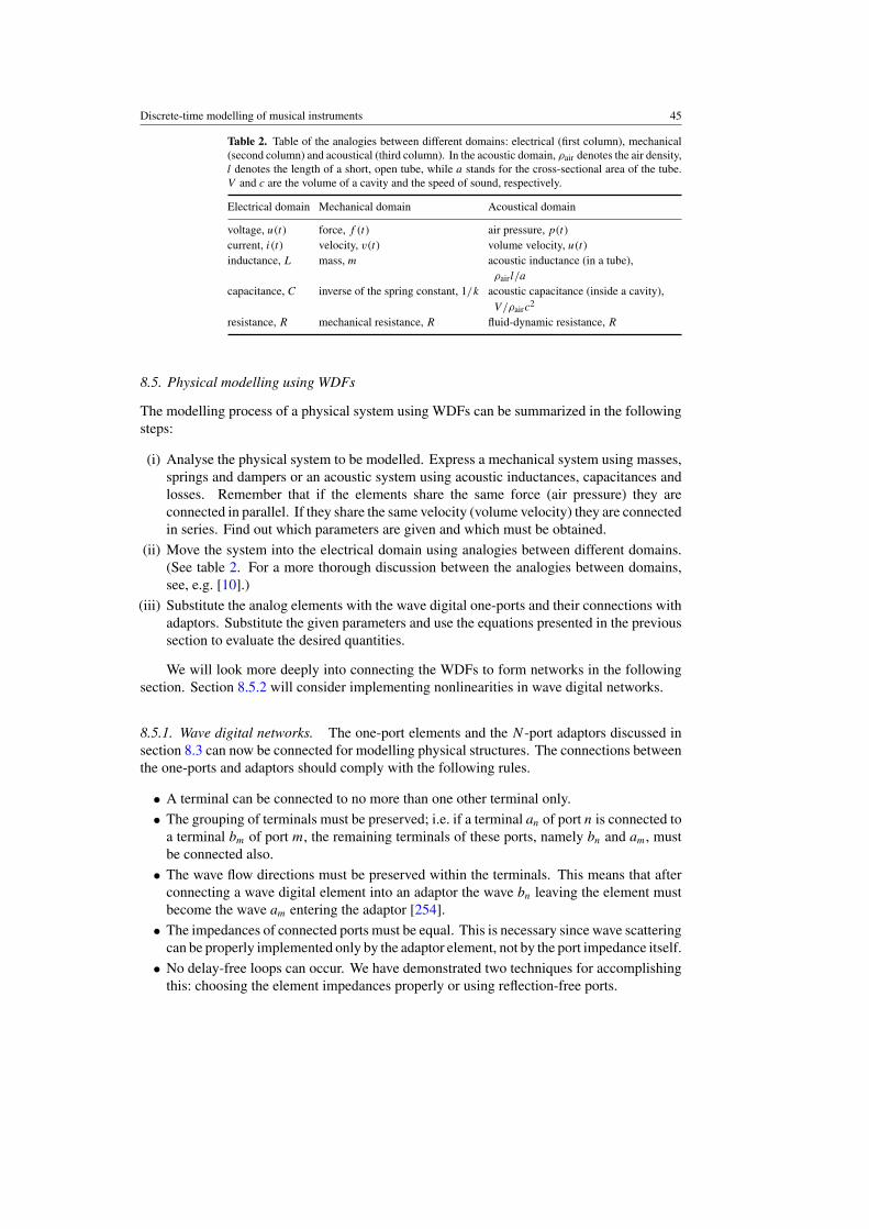
Discrete-time modelling of musical instruments 45

Table 2. Table of the analogies between different domains: electrical (first column), mechanical(second column) and acoustical (third column). In the acoustic domain, ρair denotes the air density,l denotes the length of a short, open tube, while a stands for the cross-sectional area of the tube.V and c are the volume of a cavity and the speed of sound, respectively.

Electrical domain Mechanical domain Acoustical domain

voltage, u(t) force, f (t) air pressure, p(t)

current, i(t) velocity, v(t) volume velocity, u(t)

inductance, L mass, m acoustic inductance (in a tube),ρair l/a

capacitance, C inverse of the spring constant, 1/k acoustic capacitance (inside a cavity),V/ρairc

2

resistance, R mechanical resistance, R fluid-dynamic resistance, R

8.5. Physical modelling using WDFs

The modelling process of a physical system using WDFs can be summarized in the followingsteps:

(i) Analyse the physical system to be modelled. Express a mechanical system using masses,springs and dampers or an acoustic system using acoustic inductances, capacitances andlosses. Remember that if the elements share the same force (air pressure) they areconnected in parallel. If they share the same velocity (volume velocity) they are connectedin series. Find out which parameters are given and which must be obtained.

(ii) Move the system into the electrical domain using analogies between different domains.(See table 2. For a more thorough discussion between the analogies between domains,see, e.g. [10].)

(iii) Substitute the analog elements with the wave digital one-ports and their connections withadaptors. Substitute the given parameters and use the equations presented in the previoussection to evaluate the desired quantities.

We will look more deeply into connecting the WDFs to form networks in the followingsection. Section 8.5.2 will consider implementing nonlinearities in wave digital networks.

8.5.1. Wave digital networks. The one-port elements and the N -port adaptors discussed insection 8.3 can now be connected for modelling physical structures. The connections betweenthe one-ports and adaptors should comply with the following rules.

• A terminal can be connected to no more than one other terminal only.

• The grouping of terminals must be preserved; i.e. if a terminal an of port n is connected toa terminal bm of port m, the remaining terminals of these ports, namely bn and am, mustbe connected also.

• The wave flow directions must be preserved within the terminals. This means that afterconnecting a wave digital element into an adaptor the wave bn leaving the element mustbecome the wave am entering the adaptor [254].

• The impedances of connected ports must be equal. This is necessary since wave scatteringcan be properly implemented only by the adaptor element, not by the port impedance itself.

• No delay-free loops can occur. We have demonstrated two techniques for accomplishingthis: choosing the element impedances properly or using reflection-free ports.

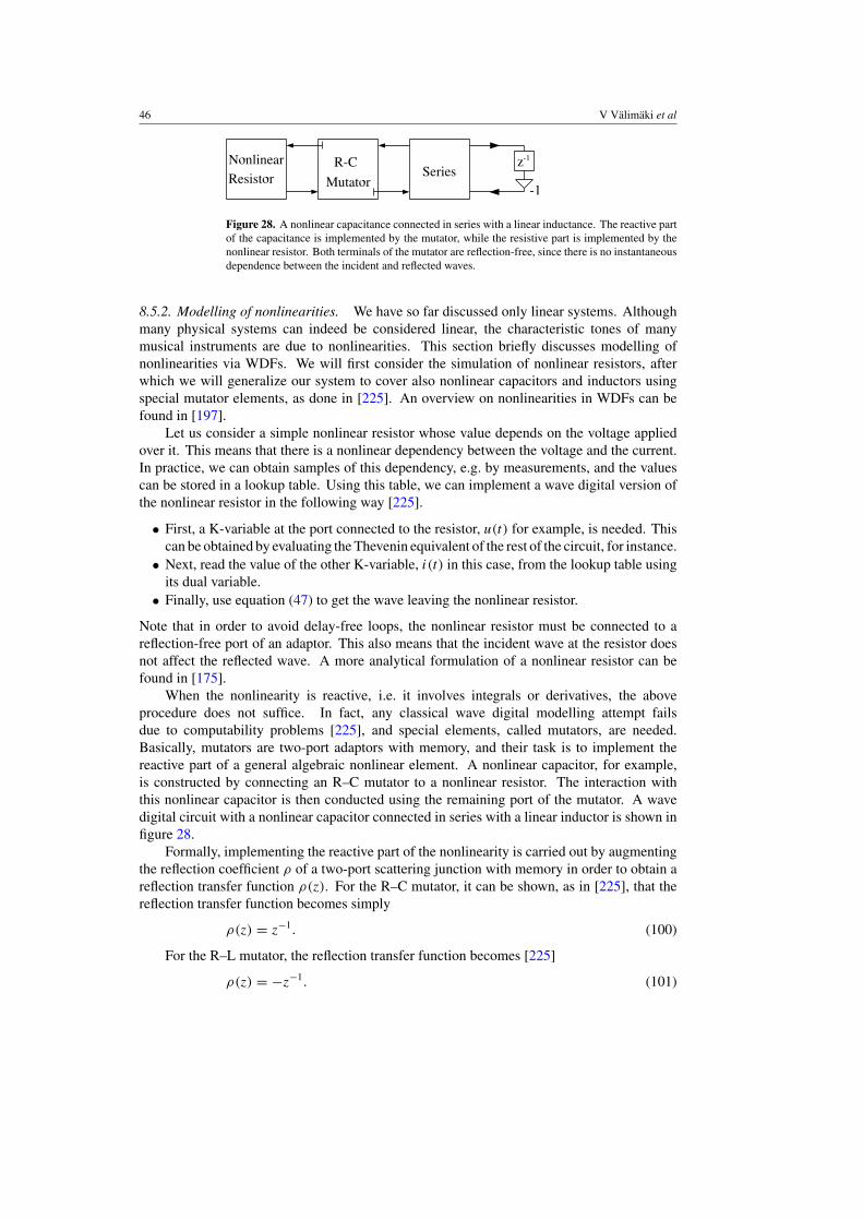
46 V Valimaki et al

Figure 28. A nonlinear capacitance connected in series with a linear inductance. The reactive partof the capacitance is implemented by the mutator, while the resistive part is implemented by thenonlinear resistor. Both terminals of the mutator are reflection-free, since there is no instantaneousdependence between the incident and reflected waves.

8.5.2. Modelling of nonlinearities. We have so far discussed only linear systems. Althoughmany physical systems can indeed be considered linear, the characteristic tones of manymusical instruments are due to nonlinearities. This section briefly discusses modelling ofnonlinearities via WDFs. We will first consider the simulation of nonlinear resistors, afterwhich we will generalize our system to cover also nonlinear capacitors and inductors usingspecial mutator elements, as done in [225]. An overview on nonlinearities in WDFs can befound in [197].

Let us consider a simple nonlinear resistor whose value depends on the voltage appliedover it. This means that there is a nonlinear dependency between the voltage and the current.In practice, we can obtain samples of this dependency, e.g. by measurements, and the valuescan be stored in a lookup table. Using this table, we can implement a wave digital version ofthe nonlinear resistor in the following way [225].

• First, a K-variable at the port connected to the resistor, u(t) for example, is needed. Thiscan be obtained by evaluating the Thevenin equivalent of the rest of the circuit, for instance.

• Next, read the value of the other K-variable, i(t) in this case, from the lookup table usingits dual variable.

• Finally, use equation (47) to get the wave leaving the nonlinear resistor.

Note that in order to avoid delay-free loops, the nonlinear resistor must be connected to areflection-free port of an adaptor. This also means that the incident wave at the resistor doesnot affect the reflected wave. A more analytical formulation of a nonlinear resistor can befound in [175].

When the nonlinearity is reactive, i.e. it involves integrals or derivatives, the aboveprocedure does not suffice. In fact, any classical wave digital modelling attempt failsdue to computability problems [225], and special elements, called mutators, are needed.Basically, mutators are two-port adaptors with memory, and their task is to implement thereactive part of a general algebraic nonlinear element. A nonlinear capacitor, for example,is constructed by connecting an R–C mutator to a nonlinear resistor. The interaction withthis nonlinear capacitor is then conducted using the remaining port of the mutator. A wavedigital circuit with a nonlinear capacitor connected in series with a linear inductor is shown infigure 28.

Formally, implementing the reactive part of the nonlinearity is carried out by augmentingthe reflection coefficient ρ of a two-port scattering junction with memory in order to obtain areflection transfer function ρ(z). For the R–C mutator, it can be shown, as in [225], that thereflection transfer function becomes simply

ρ(z) = z−1. (100)

For the R–L mutator, the reflection transfer function becomes [225]

ρ(z) = −z−1. (101)

Discrete-time modelling of musical instruments 47

(a) (b)

Figure 29. The signal flow graph of (a) the R–C mutator and (b) the R–L mutator. These graphshave been obtained from figure 26 by substituting ρ ← z−1 in (a), and ρ ← −z−1 in (b).

Note that this is in perfect agreement with our previous results; here the reflection coefficientρ of a two-port junction (see, e.g. figure 26) has just been replaced by a reflection transferfunction ρ(z), which in the case of an R–C mutator equals the reflectance of a wave digitalcapacitor (equation (53)). Similarly, for the R–L mutator, we have ρ(z) = SL(z−1). The signalflow graphs of the R–C and R–L mutators are illustrated in figure 29.

We will not consider time-varying WDFs here. Studies concerning them can be found,e.g. in [265] and [31].

8.5.3. Case study: the wave digital hammer. As a case study, we will consider a nonlinearwave digital piano hammer, introduced in [196]. This presentation of a piano hammer is asimplified one; the hammer is thought to consist of a mass and a nonlinear spring, correspondingto the compressing felt. Figure 30 shows the schematic diagram of the piano excitationmechanism, along with the simplified model. The string that the hammer excites can bemodelled using a simple digital waveguide, attached to a damper, for modelling the losses.When the hammer is in contact with the string, they must share the same velocity. Also, theforce that the hammer exerts on the string has an opposite but equal restoring force risingfrom the string, so that the total force is zero. Therefore, we can conclude that the connectionbetween the string and the hammer is a series one.

For the losses, it is clear that the string and the damper share the same velocity since theyare in motion together, and the force between them adds to zero. Therefore, the string–damperinteraction is a series connection.

For the mass-to-spring connection, although the mass and the felt both share the samevelocity when the hammer is ‘in flight’, they have different velocities when the hammer is incontact with the string, due to the felt compression. Also, since the same force is applied onboth the mass and the spring, the connection between them is parallel. With these in mind,we can now present an electrical equivalent circuit of the nonlinear piano hammer with thedamper in figure 31, and its wave digital version together with the string in figure 32.

Note that since there are no sources in this system, the wave digital hammer cannot beexcited during run time. Instead, in order to move the hammer, we must set the initial parametervalues so that the hammer is in motion already when the simulation begins.

8.5.4. Wave modelling possibilities. There are also alternative ways to perform the wavedecomposition that we did in equation (47). As already stated, current (velocity) waves couldbe used instead, which would be equivalent to changing the inductors to capacitors and serialconnections to parallel ones and vice-versa in our WDF networks. The behaviour of our modelwould still remain essentially the same, since this would mean only using the dual system inthe Kirchhoffian sense.

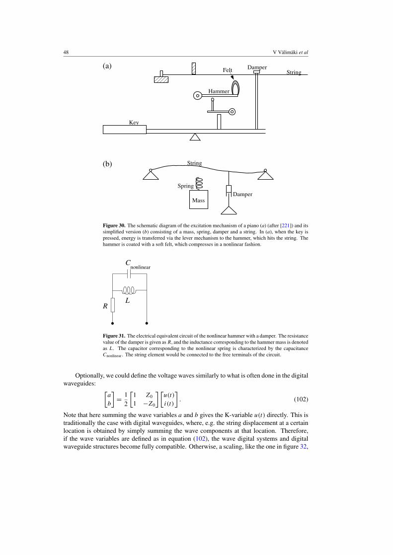
48 V Valimaki et al

Figure 30. The schematic diagram of the excitation mechanism of a piano (a) (after [221]) and itssimplified version (b) consisting of a mass, spring, damper and a string. In (a), when the key ispressed, energy is transferred via the lever mechanism to the hammer, which hits the string. Thehammer is coated with a soft felt, which compresses in a nonlinear fashion.

Figure 31. The electrical equivalent circuit of the nonlinear hammer with a damper. The resistancevalue of the damper is given as R, and the inductance corresponding to the hammer mass is denotedas L. The capacitor corresponding to the nonlinear spring is characterized by the capacitanceCnonlinear . The string element would be connected to the free terminals of the circuit.

Optionally, we could define the voltage waves similarly to what is often done in the digitalwaveguides: [

a

b

]= 1

2

[1 Z0

1 −Z0

] [u(t)

i(t)

]. (102)

Note that here summing the wave variables a and b gives the K-variable u(t) directly. This istraditionally the case with digital waveguides, where, e.g. the string displacement at a certainlocation is obtained by simply summing the wave components at that location. Therefore,if the wave variables are defined as in equation (102), the wave digital systems and digitalwaveguide structures become fully compatible. Otherwise, a scaling, like the one in figure 32,

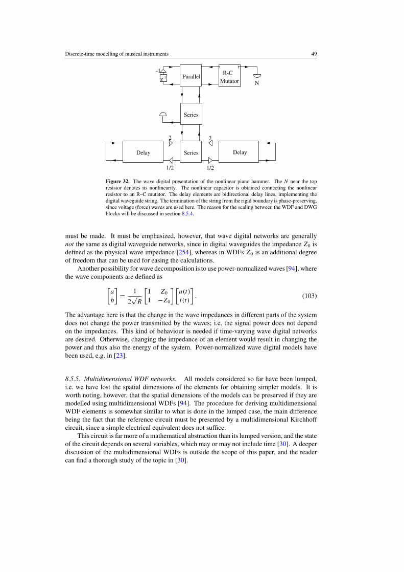
Discrete-time modelling of musical instruments 49

Figure 32. The wave digital presentation of the nonlinear piano hammer. The N near the topresistor denotes its nonlinearity. The nonlinear capacitor is obtained connecting the nonlinearresistor to an R–C mutator. The delay elements are bidirectional delay lines, implementing thedigital waveguide string. The termination of the string from the rigid boundary is phase-preserving,since voltage (force) waves are used here. The reason for the scaling between the WDF and DWGblocks will be discussed in section 8.5.4.

must be made. It must be emphasized, however, that wave digital networks are generallynot the same as digital waveguide networks, since in digital waveguides the impedance Z0 isdefined as the physical wave impedance [254], whereas in WDFs Z0 is an additional degreeof freedom that can be used for easing the calculations.

Another possibility for wave decomposition is to use power-normalized waves [94], wherethe wave components are defined as[

a

b

]= 1

2√

R

[1 Z0

1 −Z0

] [u(t)

i(t)

]. (103)

The advantage here is that the change in the wave impedances in different parts of the systemdoes not change the power transmitted by the waves; i.e. the signal power does not dependon the impedances. This kind of behaviour is needed if time-varying wave digital networksare desired. Otherwise, changing the impedance of an element would result in changing thepower and thus also the energy of the system. Power-normalized wave digital models havebeen used, e.g. in [23].

8.5.5. Multidimensional WDF networks. All models considered so far have been lumped,i.e. we have lost the spatial dimensions of the elements for obtaining simpler models. It isworth noting, however, that the spatial dimensions of the models can be preserved if they aremodelled using multidimensional WDFs [94]. The procedure for deriving multidimensionalWDF elements is somewhat similar to what is done in the lumped case, the main differencebeing the fact that the reference circuit must be presented by a multidimensional Kirchhoffcircuit, since a simple electrical equivalent does not suffice.

This circuit is far more of a mathematical abstraction than its lumped version, and the stateof the circuit depends on several variables, which may or may not include time [30]. A deeperdiscussion of the multidimensional WDFs is outside the scope of this paper, and the readercan find a thorough study of the topic in [30].

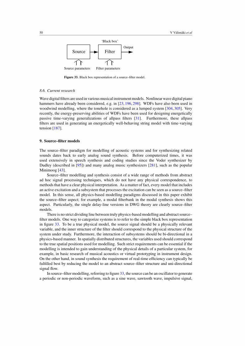
50 V Valimaki et al

FilterSourceOutput

Source parameters Filter parameters

‘Black box’

Figure 33. Black box representation of a source–filter model.

8.6. Current research

Wave digital filters are used in various musical instrument models. Nonlinear wave digital pianohammers have already been considered, e.g. in [23, 196, 298]. WDFs have also been used inwoodwind modelling, where the tonehole is considered as a lumped system [304, 305]. Veryrecently, the energy-preserving abilities of WDFs have been used for designing energeticallypassive time-varying generalizations of allpass filters [31]. Furthermore, these allpassfilters are used in generating an energetically well-behaving string model with time-varyingtension [187].

9. Source–filter models

The source–filter paradigm for modelling of acoustic systems and for synthesizing relatedsounds dates back to early analog sound synthesis. Before computerized times, it wasused extensively in speech synthesis and coding studies since the Voder synthesizer byDudley (described in [95]) and many analog music synthesizers [281], such as the popularMinimoog [43].

Source–filter modelling and synthesis consist of a wide range of methods from abstractad hoc signal processing techniques, which do not have any physical correspondence, tomethods that have a clear physical interpretation. As a matter of fact, every model that includesan active excitation and a subsystem that processes the excitation can be seen as a source–filtermodel. In this sense, all physics-based modelling paradigms discussed in this paper exhibitthe source–filter aspect; for example, a modal filterbank in the modal synthesis shows thisaspect. Particularly, the single delay-line versions in DWG theory are clearly source–filtermodels.

There is no strict dividing line between truly physics-based modelling and abstract source–filter models. One way to categorize systems is to refer to the simple black box representationin figure 33. To be a true physical model, the source signal should be a physically relevantvariable, and the inner structure of the filter should correspond to the physical structure of thesystem under study. Furthermore, the interaction of subsystems should be bi-directional in aphysics-based manner. In spatially distributed structures, the variables used should correspondto the true spatial positions used for modelling. Such strict requirements can be essential if themodelling is intended to gain understanding of the physical details of a particular system, forexample, in basic research of musical acoustics or virtual prototyping in instrument design.On the other hand, in sound synthesis the requirement of real-time efficiency can typically befulfilled best by reducing the model to an abstract source–filter structure and uni-directionalsignal flow.

In source–filter modelling, referring to figure 33, the source can be an oscillator to generatea periodic or non-periodic waveform, such as a sine wave, sawtooth wave, impulsive signal,

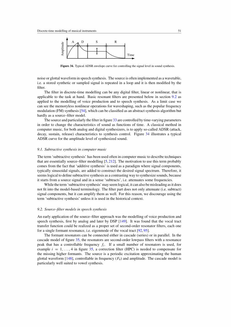
Discrete-time modelling of musical instruments 51

TimeAm

plitu

de

A D

Figure 34. Typical ADSR envelope curve for controlling the signal level in sound synthesis.

noise or glottal waveform in speech synthesis. The source is often implemented as a wavetable,i.e. a stored synthetic or sampled signal is repeated in a loop and it is then modified by thefilter.

The filter in discrete-time modelling can be any digital filter, linear or nonlinear, that isapplicable to the task at hand. Basic resonant filters are presented below in section 9.2 asapplied to the modelling of voice production and to speech synthesis. As a limit case wecan see the memoryless nonlinear operations for waveshaping, such as the popular frequencymodulation (FM) synthesis [54], which can be classified as an abstract synthesis algorithm buthardly as a source–filter model.

The source and particularly the filter in figure 33 are controlled by time-varying parametersin order to change the characteristics of sound as functions of time. A classical method incomputer music, for both analog and digital synthesizers, is to apply so-called ADSR (attack,decay, sustain, release) characteristics to synthesis control. Figure 34 illustrates a typicalADSR curve for the amplitude level of synthesized sound.

9.1. Subtractive synthesis in computer music

The term ‘subtractive synthesis’ has been used often in computer music to describe techniquesthat are essentially source–filter modelling [5, 212]. The motivation to use this term probablycomes from the fact that ‘additive synthesis’ is used as a paradigm where signal components,typically sinusoidal signals, are added to construct the desired signal spectrum. Therefore, itseems logical to define subtractive synthesis as a contrasting way to synthesize sounds, becauseit starts from a source signal and in a sense ‘subtracts’, i.e. attenuates some frequencies.

While the term ‘subtractive synthesis’ may seem logical, it can also be misleading as it doesnot fit into the model-based terminology. The filter part does not only attenuate (i.e. subtract)signal components, but it can amplify them as well. For this reason, we discourage using theterm ‘subtractive synthesis’ unless it is used in the historical context.

9.2. Source–filter models in speech synthesis

An early application of the source–filter approach was the modelling of voice production andspeech synthesis, first by analog and later by DSP [149]. It was found that the vocal tracttransfer function could be realized as a proper set of second-order resonator filters, each onefor a single formant resonance, i.e. eigenmode of the vocal tract [92, 95].

The formant resonators can be connected either in cascade (series) or in parallel. In thecascade model of figure 35, the resonators are second-order lowpass filters with a resonancepeak that has a controllable frequency fi . If a small number of resonators is used, forexample i = 1, . . . , 4 in figure 35, a correction filter (HPC) is needed to compensate forthe missing higher formants. The source is a periodic excitation approximating the humanglottal waveform [148], controllable in frequency (F0) and amplitude. The cascade model isparticularly well suited to vowel synthesis.

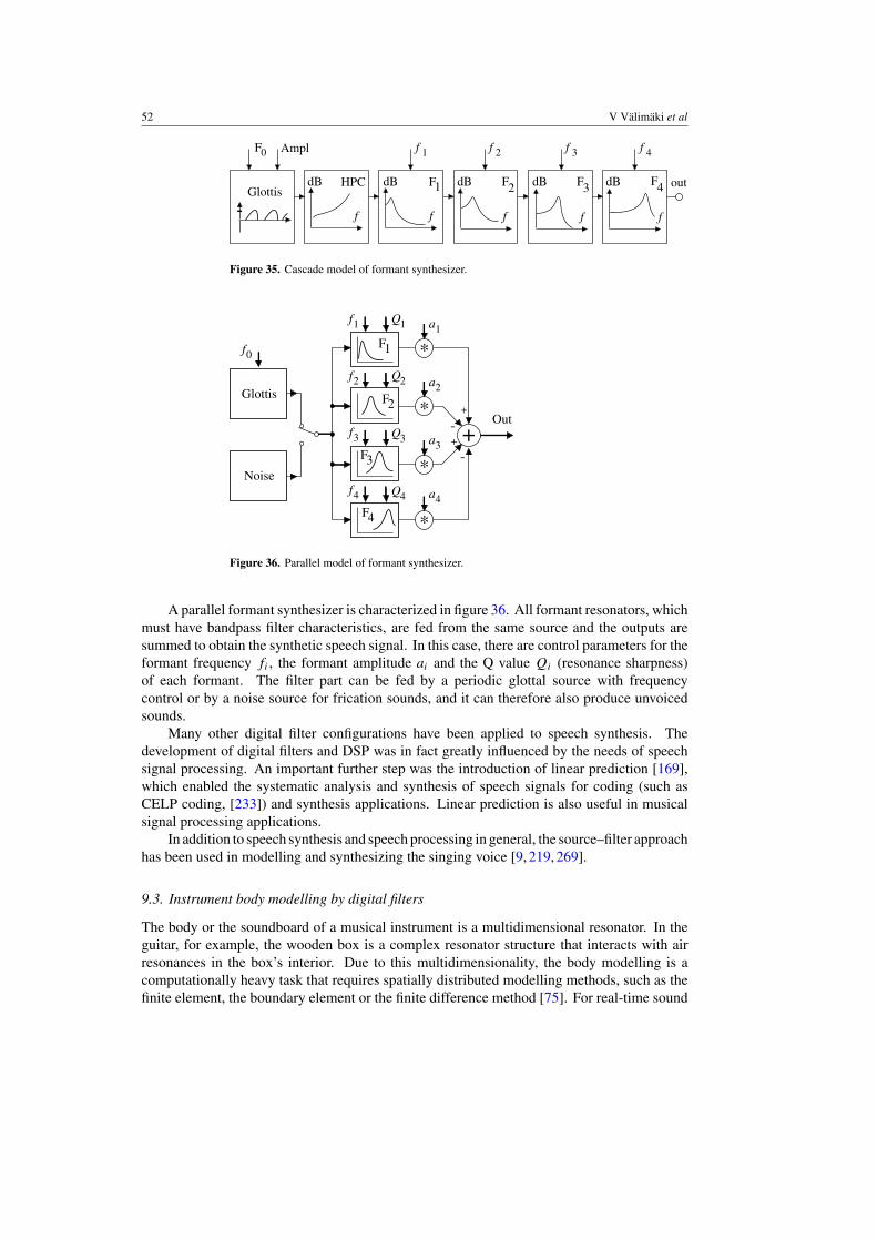
52 V Valimaki et al

F0 Ampl 1f 2f 3f 4f

GlottisF4

f f f f

dBdBdBdBdB

f

F1 F2 F3 F4HPC out

Figure 35. Cascade model of formant synthesizer.

*

*

*

*

+

Glottis

Noise

F1

F2

F3

F4

1f 1a

2a

3a

4a

1Q

2Q

3Q

4Q

0f

2f

3f

4f

+

-+

-

Out

Figure 36. Parallel model of formant synthesizer.

A parallel formant synthesizer is characterized in figure 36. All formant resonators, whichmust have bandpass filter characteristics, are fed from the same source and the outputs aresummed to obtain the synthetic speech signal. In this case, there are control parameters for theformant frequency fi , the formant amplitude ai and the Q value Qi (resonance sharpness)of each formant. The filter part can be fed by a periodic glottal source with frequencycontrol or by a noise source for frication sounds, and it can therefore also produce unvoicedsounds.

Many other digital filter configurations have been applied to speech synthesis. Thedevelopment of digital filters and DSP was in fact greatly influenced by the needs of speechsignal processing. An important further step was the introduction of linear prediction [169],which enabled the systematic analysis and synthesis of speech signals for coding (such asCELP coding, [233]) and synthesis applications. Linear prediction is also useful in musicalsignal processing applications.

In addition to speech synthesis and speech processing in general, the source–filter approachhas been used in modelling and synthesizing the singing voice [9, 219, 269].

9.3. Instrument body modelling by digital filters

The body or the soundboard of a musical instrument is a multidimensional resonator. In theguitar, for example, the wooden box is a complex resonator structure that interacts with airresonances in the box’s interior. Due to this multidimensionality, the body modelling is acomputationally heavy task that requires spatially distributed modelling methods, such as thefinite element, the boundary element or the finite difference method [75]. For real-time sound

Discrete-time modelling of musical instruments 53

Delay line (wavetable)

Loop Filter 0.5(1+z-1)x(n)y(n)

Output x(n)

Figure 37. Signal flow diagram of Karplus–Strong algorithm.

synthesis, these methods are in most cases computationally too expensive. Thus, it is attractiveto try to reduce the body effect to a single digital filter.

A number of filter-based body models were introduced in [139]. These include frequency-warped filters [108] and several basic techniques of filter decompositions. Since the modelswith full auditory accuracy tend to be expensive even for today’s computers, simplificationsare desirable. Higher frequency modes can be made sparse or totally discarded or they maybe approximated by a reverberation algorithm [117, 198].

9.4. The Karplus–Strong algorithm

The Karplus–Strong algorithm is one of the basic inventions in computer music that later turnedout to be an interesting and extremely simplified case of a physics-based model as well as akind of source–filter. A wavetable is first filled with data, such as random numbers. Then it iscirculated like the single delay-line loop with a simple loop filter, see figure 37. This methodwas proposed by Karplus and Strong [144], and soon thereafter it was extended to forms thathave a closer relationship to physics-based modelling [120, 143, 244].

In the original Karplus–Strong algorithm, the loop filter is an averager of two succeedingsamples, which corresponds to the transfer function H(z) = 0.5 (1 + z−1) and works asa lowpass filter. Thus, the filter attenuates high frequencies in the loop faster than lowfrequencies, which is exactly what happens, for example, in a plucked string. A new soundcan be started by loading new content into the delay line. The fundamental frequency caneasily be changed by controlling the sample rate of computation or the length of the delay line.Due to the extreme simplicity of the algorithm, it enabled real-time sound synthesis using thecomputers and processors of the early 1980s.

By feeding the excitation into the model from the dashed line input in figure 37 insteadof loading the delay line all at once, the algorithm is converted into a source–filter structure.Through various extensions, it has been turned into different practical sound synthesis models,as discussed in section 7.

9.5. Virtual analog synthesis

Digital subtractive synthesis is called virtual analog synthesis, when reference is made tocomputational methods that imitate the sound generation principles of analog synthesizers ofthe 1960s and 1970s. The term ‘virtual analog synthesis’ became a popular and commercialterm around 1995, when a Swedish company called Clavia introduced the Nord Lead 1synthesizer, which was marketed as an analog-sounding digital synthesizer that used nosampled sounds. Instead, all of its sounds were generated by simulating analog subtractivesynthesis using DSP techniques. Previously, the Roland D-50 synthesizer of the late 1980sworked in a similar way, although it also used sampled sounds. An early example of an attemptto design an analog-sounding digital synthesizer was the Synergy synthesizer [126].

What makes digital subtractive synthesis more demanding than is generally understoodis that imitating analog electronics with digital processing is not as easy as it may seem.

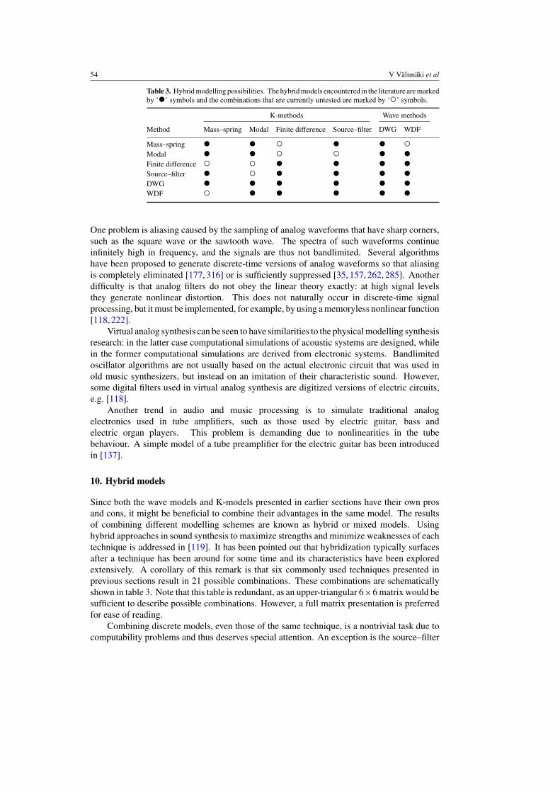
54 V Valimaki et al

Table 3. Hybrid modelling possibilities. The hybrid models encountered in the literature are markedby ‘•’ symbols and the combinations that are currently untested are marked by ‘◦’ symbols.

K-methods Wave methods

Method Mass–spring Modal Finite difference Source–filter DWG WDF

Mass–spring • • ◦ • • ◦Modal • • ◦ ◦ • •Finite difference ◦ ◦ • • • •Source–filter • ◦ • • • •DWG • • • • • •WDF ◦ • • • • •

One problem is aliasing caused by the sampling of analog waveforms that have sharp corners,such as the square wave or the sawtooth wave. The spectra of such waveforms continueinfinitely high in frequency, and the signals are thus not bandlimited. Several algorithmshave been proposed to generate discrete-time versions of analog waveforms so that aliasingis completely eliminated [177, 316] or is sufficiently suppressed [35, 157, 262, 285]. Anotherdifficulty is that analog filters do not obey the linear theory exactly: at high signal levelsthey generate nonlinear distortion. This does not naturally occur in discrete-time signalprocessing, but it must be implemented, for example, by using a memoryless nonlinear function[118, 222].

Virtual analog synthesis can be seen to have similarities to the physical modelling synthesisresearch: in the latter case computational simulations of acoustic systems are designed, whilein the former computational simulations are derived from electronic systems. Bandlimitedoscillator algorithms are not usually based on the actual electronic circuit that was used inold music synthesizers, but instead on an imitation of their characteristic sound. However,some digital filters used in virtual analog synthesis are digitized versions of electric circuits,e.g. [118].

Another trend in audio and music processing is to simulate traditional analogelectronics used in tube amplifiers, such as those used by electric guitar, bass andelectric organ players. This problem is demanding due to nonlinearities in the tubebehaviour. A simple model of a tube preamplifier for the electric guitar has been introducedin [137].

10. Hybrid models

Since both the wave models and K-models presented in earlier sections have their own prosand cons, it might be beneficial to combine their advantages in the same model. The resultsof combining different modelling schemes are known as hybrid or mixed models. Usinghybrid approaches in sound synthesis to maximize strengths and minimize weaknesses of eachtechnique is addressed in [119]. It has been pointed out that hybridization typically surfacesafter a technique has been around for some time and its characteristics have been exploredextensively. A corollary of this remark is that six commonly used techniques presented inprevious sections result in 21 possible combinations. These combinations are schematicallyshown in table 3. Note that this table is redundant, as an upper-triangular 6×6 matrix would besufficient to describe possible combinations. However, a full matrix presentation is preferredfor ease of reading.

Combining discrete models, even those of the same technique, is a nontrivial task due tocomputability problems and thus deserves special attention. An exception is the source–filter

Discrete-time modelling of musical instruments 55

technique, because it is based on unidirectional signal flow as opposed to a dual pair ofvariables. It is therefore possible to combine the source–filter technique with any othertechnique, although such a combination is not common in modal synthesis.

The wave-based methods are more apt to hybrid modelling, as the WDF and DWGstructures are mostly compatible. In addition, the adaptors in WDFs and the isomorphicscattering junctions in DWGs readily eliminate the delay-free loops in LTI cases. Because ofthese desirable properties, many WDF–DWG hybrids are reported in the literature (see, forinstance, the hybrid model of a wave digital piano hammer and a DWG string in section 8and the woodwind hybrid model reported in [304]). Moreover, the generalized theory ofmultivariable waveguides and scattering allows expression of DWG networks in a compactway [218]. The time-varying and nonlinear cases require special methods, as will be outlinedin the next section.

The interconnected K-modules usually contain delay-free loops. We have already seen anexample of how a delay-free loop occurs when linking two mass elements in section 5. Thereported hybrid K-models usually restore computability by inserting a unit delay within thedelay-free loop. This additional delay usually affects the accuracy and stability of the resultinghybrid structure, as demonstrated in a numerical model of hammer–string interaction in [33].An exceptional case occurs when one of the interconnected K-modules has an impulse responsethat satisfies h(0) = 0. The output of such a module depends only on the past values of itsinputs, which essentially means that a delay-free loop does not occur and the computability isrestored without an additional delay, as reported in [105].

In this section we focus on systematic approaches for constructing hybrid models thatinherently address the computability, accuracy, stability and efficiency of the resulting structure.A general method for solving computability problems due to the delay-free loops, especiallythose found when connecting nonlinear excitation blocks to linear resonator blocks, has beenreported in [33]. This method is called the ‘K-method’ since it operates on the K-variablesrather than the wave variables. The K-method transforms the state-variables of the linearpart of the system in order to indicate all delay-free loops involving nonlinear maps andthen operates a geometrical transformation on the nonlinearities in order to cut instantaneousdependences. Two possibilities are available for efficient numerical implementation of theK-method. The first is to pre-compute the new nonlinear map off-line and store it in a lookuptable. Alternatively, it can be iteratively computed using the Newton–Raphson method. Theiterative method has been used for combining two modal resonators and implementing theirnonlinear interaction in [215].

10.1. KW-hybrids

In this section, we consider the connection of the wave models with K-models. We use theshorthand ‘KW-hybrid’ to refer to this kind of hybrid model.

The K-method can be used to form a KW-hybrid to couple a nonlinear lumped hammermodel (consisting of a mass and a nonlinear spring) to a DWG [33]. In the case of LTImodels, the K-method simplifies significantly, as the geometrical transformation can be solvedanalytically. Even simpler approaches have been reported for systematically constructedKW-hybrids.

One way of constructing KW-hybrids is to formulate a particular modular K-modelwith explicit instantaneous interaction elements and then use a special KW-converter. TheKW-converter concept was developed in [80, 132] and formalized in [131]. The advantageof this approach is that the full dynamics of the K-model are preserved and its schedulingis made similar to that of the wave model. The disadvantage of this approach is that it is

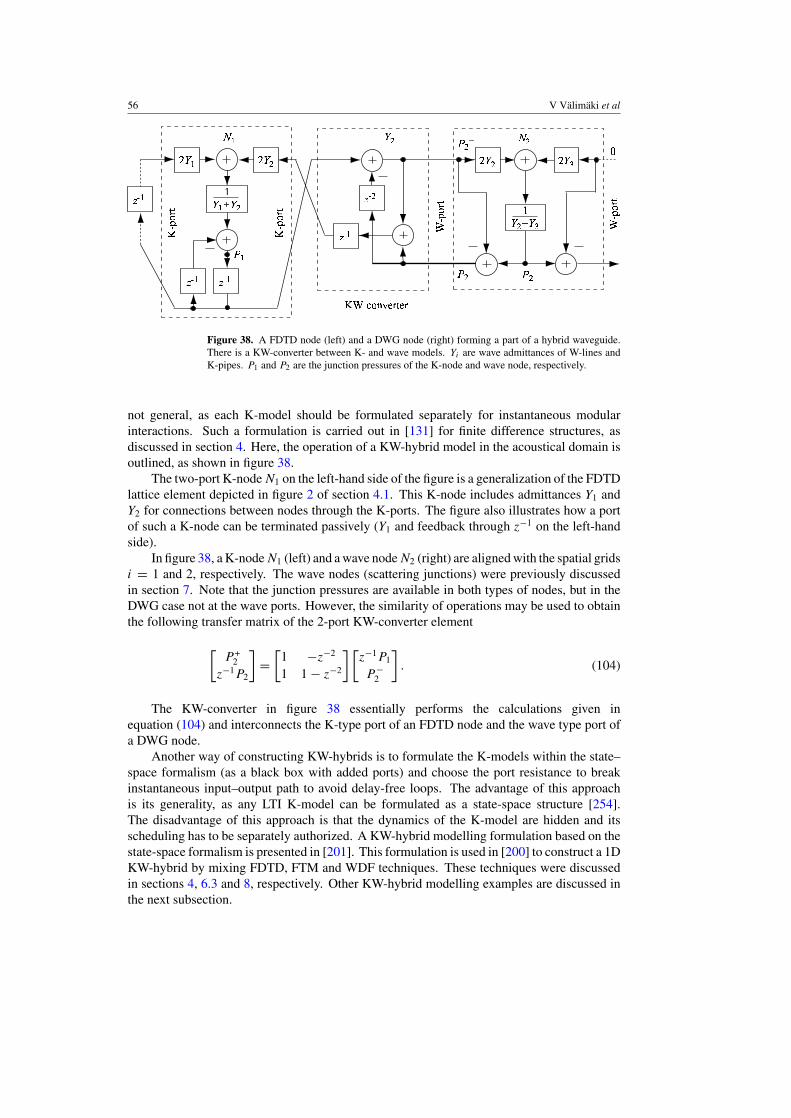
56 V Valimaki et al

Figure 38. A FDTD node (left) and a DWG node (right) forming a part of a hybrid waveguide.There is a KW-converter between K- and wave models. Yi are wave admittances of W-lines andK-pipes. P1 and P2 are the junction pressures of the K-node and wave node, respectively.

not general, as each K-model should be formulated separately for instantaneous modularinteractions. Such a formulation is carried out in [131] for finite difference structures, asdiscussed in section 4. Here, the operation of a KW-hybrid model in the acoustical domain isoutlined, as shown in figure 38.

The two-port K-node N1 on the left-hand side of the figure is a generalization of the FDTDlattice element depicted in figure 2 of section 4.1. This K-node includes admittances Y1 andY2 for connections between nodes through the K-ports. The figure also illustrates how a portof such a K-node can be terminated passively (Y1 and feedback through z−1 on the left-handside).

In figure 38, a K-node N1 (left) and a wave node N2 (right) are aligned with the spatial gridsi = 1 and 2, respectively. The wave nodes (scattering junctions) were previously discussedin section 7. Note that the junction pressures are available in both types of nodes, but in theDWG case not at the wave ports. However, the similarity of operations may be used to obtainthe following transfer matrix of the 2-port KW-converter element

[P +

2

z−1P2

]=

[1 −z−2

1 1 − z−2

] [z−1P1

P −2

]. (104)

The KW-converter in figure 38 essentially performs the calculations given inequation (104) and interconnects the K-type port of an FDTD node and the wave type port ofa DWG node.

Another way of constructing KW-hybrids is to formulate the K-models within the state–space formalism (as a black box with added ports) and choose the port resistance to breakinstantaneous input–output path to avoid delay-free loops. The advantage of this approachis its generality, as any LTI K-model can be formulated as a state-space structure [254].The disadvantage of this approach is that the dynamics of the K-model are hidden and itsscheduling has to be separately authorized. A KW-hybrid modelling formulation based on thestate-space formalism is presented in [201]. This formulation is used in [200] to construct a 1DKW-hybrid by mixing FDTD, FTM and WDF techniques. These techniques were discussedin sections 4, 6.3 and 8, respectively. Other KW-hybrid modelling examples are discussed inthe next subsection.

Discrete-time modelling of musical instruments 57

10.2. KW-hybrid modelling examples

A practical application utilizing a KW-hybrid model is the RoomWeaver [20]; a softwareapplication used for building virtual 3D spaces and modelling their room impulse responses.RoomWeaver utilizes rectangular (2D) or cubic arrays (3D) of digital waveguide meshes tomodel the space with the desired geometry. Since multidimensional finite difference structuresare computationally more efficient but do not provide as good implementations for boundaryconditions as DWG schemes do, a mixed model is the proper choice for large meshes. InRoomWeaver, a KW-hybrid model (constructed by using the KW-converters in figure 38) isused to accomplish an efficient modelling solution. A comparison of the hybrid modelling andthe conventional approaches is performed in [20]. A fan-shaped room was simulated at thesampling rate of 44.1 kHz using 260330 nodes in a mesh. The results showed a speed increaseof 200% and a memory usage decrease of 50% when the hybrid mesh was compared withthe standard one.

Other examples of FDTD/DWG hybrids include the string collision model ofKrishnaswamy and Smith [153] and the finite width bow/string model of Pitteroff andWoodhouse [203–205]. These models are discussed in sections 11.1.4 and 7, respectively.

11. Modelling of nonlinear and time-varying phenomena

All musical instruments experience nonlinear behaviour. In some cases, the effect that thenonlinearity imparts on the sound of the instrument is so small that it can be considerednegligible, and a linear synthesis model will suffice. For many instruments, however, this isnot the case. All musical instruments also possess more or less time-variant properties. Thisis due to control by the player: the pitch or timbre of an instrument must usually vary in timein order for the sound to be considered musically interesting. Modelling of the time-varyingphenomena can be achieved in two ways. The simplest choice is to use several copies ofthe same synthesis engine with different parameters to produce the different tones. This isespecially well suited to the case in which the change in pitch or timbre is more instantaneousthan gradual, e.g. in the case of a piano model. For instruments that experience a gradualchange in sound characteristics, such as the slide guitar or a violin, a single synthesis modelwith time-varying properties must be used.

Modelling of nonlinear and time-varying phenomena will nearly always increase thecomputational complexity of the synthesis algorithm, since common simplifications, such ascommuting, are no longer theoretically valid and thus usually cannot be applied. The followingsection will briefly discuss the modelling of different nonlinear phenomena in musicalinstruments. For an excellent overview of nonlinearities in musical instruments, see [97] andfor the physics of musical instruments in general, see [96]. Section 11.2 will provide a moredetailed case study in modelling the spatially distributed nonlinear string using a novel energy-preserving technique. Section 11.3 will discuss the modelling of time-varying properties ofmusical instruments with a special focus on energy conservation and stability issues.

11.1. Modelling of nonlinearities in musical instruments

11.1.1. Bowed strings. The nonlinearity in bowed string instruments is one of the mostextensively studied musical instrument phenomena [68, 174, 203, 234, 236, 237, 321]. Inbowed strings, as in all sustained tone instruments, the generation of harmonic tones requiresnonlinear behaviour from the excitation mechanism [97]. In this case, the nonlinearity lies inthe stick–slip contact between the bow and the string.

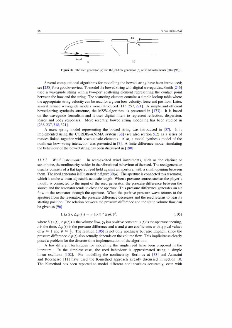
58 V Valimaki et al

Figure 39. The reed generator (a) and the jet-flow generator (b) of wind instruments (after [96]).

Several computational algorithms for modelling the bowed string have been introduced;see [238] for a good overview. To model the bowed string with digital waveguides, Smith [246]used a waveguide string with a two-port scattering element representing the contact pointbetween the bow and the string. The scattering element contains a simple lookup table wherethe appropriate string velocity can be read for a given bow velocity, force and position. Later,several refined waveguide models were introduced [115, 257, 271]. A simple and efficientbowed-string synthesis structure, the MSW-algorithm, is presented in [173]. It is basedon the waveguide formalism and it uses digital filters to represent reflection, dispersion,losses and body responses. More recently, bowed string modelling has been studied in[236, 237, 318, 321].

A mass–spring model representing the bowed string was introduced in [37]. It isimplemented using the CORDIS-ANIMA system [38] (see also section 5.2) as a series ofmasses linked together with visco-elastic elements. Also, a modal synthesis model of thenonlinear bow–string interaction was presented in [7]. A finite difference model simulatingthe behaviour of the bowed string has been discussed in [190].

11.1.2. Wind instruments. In reed-excited wind instruments, such as the clarinet orsaxophone, the nonlinearity resides in the vibrational behaviour of the reed. The reed generatorusually consists of a flat tapered reed held against an aperture, with a small opening betweenthem. The reed generator is illustrated in figure 39(a). The aperture is connected to a resonator,which is a tube with an adjustable acoustic length. When a pressure source, such as the player’smouth, is connected to the input of the reed generator, the pressure difference between thesource and the resonator tends to close the aperture. This pressure difference generates an airflow to the resonator through the aperture. When the positive pressure wave returns to theaperture from the resonator, the pressure difference decreases and the reed returns to near itsstarting position. The relation between the pressure difference and the static volume flow canbe given as [96]

U(x(t), p(t)) = γ1|x(t)|α p(t)β, (105)

where U(x(t), p(t)) is the volume flow, γ1 is a positive constant, x(t) is the aperture opening,t is the time, p(t) is the pressure difference and α and β are coefficients with typical valuesof α ≈ 1 and β ≈ 1

2 . The relation (105) is not only nonlinear but also implicit, since thepressure difference p(t) also actually depends on the volume flow. This implicitness clearlyposes a problem for the discrete-time implementation of the algorithm.

A few different techniques for modelling the single reed have been proposed in theliterature. In the simplest case, the reed behaviour is approximated using a simplelinear oscillator [102]. For modelling the nonlinearity, Borin et al [33] and Avanziniand Rocchesso [11] have used the K-method approach already discussed in section 10.The K-method has been reported to model different nonlinearities accurately, even with

Discrete-time modelling of musical instruments 59

low sampling rates [15, 33]. A computationally demanding finite difference approachfor directly discretizing the nonlinear reed equations was introduced in [291]. In 1986,Smith [246] proposed a conceptually straightforward waveguide method for synthesizing areed instrument. In this model, the reed has been implemented as a simple lookup table,where the nonlinear relationship between the flow and the pressure has been stored in advance.This computationally efficient method is able to produce relatively high-quality synthesis.A spatially distributed reed model, that is, a model that does not consider the reed as a lumped,pointlike element, has been discussed in [13]. Very recently, Guillemain and co-workers [105]have shown that equation (105) can be solved explicitly in discrete time.

Modelling of the more complicated excitation mechanism, the nonlinear double reed, isdiscussed, for example, in [106, 311]. The double reed is used as an excitor in the oboe andbassoon, for example.

In brass instruments, such as the trumpet or trombone, the excitation mechanism, i.e. theplayer’s lips, behaves somewhat differently from the reed. Several models for explainingthe behaviour of the lip–valve excitors have been proposed. A review paper can be foundin [40]. Sound synthesis based on such models has been discussed by several authors[1, 76, 180, 220, 313].

In jet-flow type wind instruments, such as the flute or the recorder, the resonator is excitedby an air flow instead of a vibrating reed. When the pressure source is connected to thegenerator, the air jet emerges from a flue slit, passes the embouchure hole and finally reachesthe bore edge, as illustrated in figure 39(b). The jet stream clearly generates a pressure waveinside the bore. When the pressure maximum returns to the slit end, it pushes the jet streamaway from the bore. In other words, the moving air inside the bore modulates the transversaldisplacement of the jet stream, which in turn excites the air in the bore. With suitable borelengths and jet velocities, this coupled air movement turns into a sustained oscillation. The airflow into the resonator can be given as [96]

U( h(t)) = WbV

(tanh

( h(t)

b

)+ 1

), (106)

where W , b and V are parameters defining the shape of the jet stream and h(t) is the time-varying transverse offset between the jet and the slit. As can be seen, equation (106) is alsononlinear. The behaviour of the jet flue is studied more thoroughly, for example, in [309].A review paper about lumped jet flue models can be found in [91].

The flute synthesis models presented in the literature are surprisingly similar in nature. Inalmost all cases, digital waveguides have been used for modelling the instrument bore, whilethe nonlinearity has been realized with a lookup table or a simple polynomial. A signal delayis inserted prior to the nonlinearity for modelling the time it takes for the jet flow to travelacross the embouchure hole.

The general requirements for a computational time-domain flute model were alreadydiscussed in [173]. The first real-time synthesis model was briefly presented by Karjalainenet al in [135]. It implemented the nonlinearity with a sigmoid function. A refined model wasproposed in [288], where scaling coefficients for the pressure input and the feedback fromthe bore were added. Soon after that another waveguide model with a simple polynomialsimulating the nonlinearity [61] and a conceptually similar model with a physically morerigorous approach were presented [55]. Chaotic variations in the jet offset due to turbulencehave been simulated by slightly varying the coefficients of the polynomial nonlinearity witha noise generator [44, 62]. A waveguide-based flutelike instrument model, which takes intoaccount the vortex shedding at the slit edge (labium) and the turbulence at the mouth of theinstrument, has been proposed in [310].

60 V Valimaki et al

11.1.3. The Piano. In a piano, the sound is generated when the player presses a key. Themovement is transferred via a jack into the piano hammer, which hits the piano string (there areactually multiple strings for a hammer especially in the treble end, but here we will considerthe case of a single string for the sake of simplicity). See figure 30 in section 8.5.3 for anillustration. For a more thorough discussion on piano acoustics, see, e.g. [96].

The piano hammer is basically a piece of wood covered with a layer of felt. Thecompression characteristics of the felt are inherently nonlinear, which affects the generatedtone. This passive nonlinearity manifests itself when the piano is played with varying dynamics.When playing with greater intensity ( fortissimo), the hammer seems harder than if the pianowere played softly ( pianissimo). This change of the effective stiffness results in greateramplitude of the higher harmonics, i.e. the sound is brighter if the piano is played with greaterintensity.

When modelling the piano hammer, the core of the hammer is often simplified as a lumpedmass while the felt is presented as a nonlinear spring connected to this mass. The force-to-compression relationship of this mass–spring system can be presented as [107]

F( y(t)) = C−1 y(t)p, (107)

when the hammer is in contact with the string. Here, F( y(t)) denotes the force applied tothe string by the hammer, y(t) is the compression of the spring (felt) and C is its generalizedcompliance. Note that with p = 1, equation (107) becomes Hooke’s law for springs (22).Interestingly, the compression of the felt depends in turn on the hammer force, so equation (107)is implicit.

Several synthesis models for piano hammer–string interaction have been suggested; see[15] for a review. Chaigne and Askenfelt [46,47] have used the finite difference discretizationof equation (107) with an additional delay between the compression and force terms in orderto force the relation explicit. This artificial delay, however, makes the synthesis algorithmpotentially unstable [15]. The K method [33] discussed earlier has also been utilized inremoving the implicitness of equation (107). Very recently, Bensa and co-workers [26] havestudied the parameter fitting for the hammer–string model.

As discussed in section 8, WDFs hold special means for removing the delay-free loops andhave thus also been used in modelling the nonlinear piano hammer [23, 196, 225, 298]. Smithand Van Duyne [258, 301] have introduced a computationally efficient commuted waveguidemodel wherein the hammer is implemented as a linear filter. When the hammer hits thestring, an impulse is fed to the string through this filter. The filter parameters are read from apre-calculated table for a given hammer velocity.

There is also an additional physical phenomenon taking place in the compressingfelt, namely the hysteresis. During interaction with the strings, the felt compresses andrelaxes several times due to the travelling displacement wave in the string [34]. Thehysteresis takes place when the temporal derivative of the felt compression changes itssign. In other words, when the compression of the felt starts to relax, the compression-to-force relationship does not follow the same trajectory as it did when the compression wasincreasing. In order to model the hysteresis effect also, Boutillon [34] suggested that amodel

F(y) ={ai yαi when y increases,ad yαd when y decreases,

(108)

be used. Here, F(y) is the force applied by the hammer to a rigid string, y is the hammerfelt deformation and a and α represent a hypothetical series of coefficients, where each a andα must be larger than its predecessor.

Discrete-time modelling of musical instruments 61

11.1.4. Plucked string instruments. Plucked string instruments experience two main typesof nonlinearities. The first is hard-limitation nonlinearity, which takes place when a freelyvibrating string hits a spatial obstacle. The obstacle obviously limits the amplitude of thevibration, producing a nonlinear ‘clipping’ of the vibration. Usually, the obstacle is a part ofthe instrument itself, such as in the case of slapbass, where the string is ‘popped’ or struckso hard that it hits the frets on the fingerboard. A more complex manifestation of the hard-limitation nonlinearity takes place, e.g. in the Indian sitar or the tanpura. In these cases, theunilateral constraint caused by the curved bridge effectively shortens the string as it displacestowards the bridge [254]. A more thorough discussion of the effect is provided in [282].

The hard-limitation nonlinearity in the case of the slapbass was first modelled by Rankand Kubin in the late nineties [208]. They used a waveguide string model with displacementsignals as wave variables. During the vibration, the displacement of the string is probed incertain given points on the string and then compared with the displacement limit yfret, i.e. thedistance between the string and the fret in equilibrium. If the string displacement exceedsthe limit value at some of these locations, the displacement waves are reflected (with a signchange) into the delay line travelling in the opposite direction. When the displacement limitvalue is added to this, the string vibration amplitude at any of the given points is limited to yfret.

Later, Karjalainen [127] suggested a technique where an impulse with a suitable amplitudeis fed into the string when the collision with the obstacle occurs. This operation is in factidentical to what is described in [208], although it provides an alternative representation forthe string by using so-called FDTD waveguides, illustrated already in figure 2. Soon after,Krishnaswamy and Smith [153] pointed out a nonphysical feature in the simulated string whenthis technique is used. They observed that the string release from the obstacle happens laterthan physical laws would predict, as if the string had artificial ‘stickiness’. They formulateda refined waveguide model for the hard-limitation nonlinearity, which removed the constantoffset differences between the two waveguide segments and thus resolved the physical validityproblem. In addition to this computationally more expensive waveguide model, a FDTD/DWGhybrid approach was introduced in [153].

The other main nonlinearity in plucked strings resides in the variation of string tension dueto transversal vibration. It has been extensively studied in the literature [6, 41, 179, 183, 184].When a string is displaced, its tension is also increased. When the string moves near itsequilibrium position, the tension is decreased. It is easy to see that the tension variation hastwice the frequency of the transversal vibration, since both extreme displacements of the stringproduce a tension maximum, and the tension minimum is obtained when the string is near itssteady-state location. With this in mind, it is also easy to understand that since a real stringvibration decays in time, the average string tension also has a decaying form. As stated inequation (6), this tension decay leads into a decay in wave velocities and a descent in thefundamental frequency of the string.

This phenomenon, called the initial pitch glide, is most apparent in elastic strings withhigh vibrational amplitudes and relatively low nominal tension. In fact, the pitch glide is notthe only effect caused by tension modulation. As is well known, the lack of certain modesin a plucked string vibration occurs due to the plucking location, which heavily attenuatesall harmonics that would have a node at that point. In an ideal mid-plucked string, forexample, all even modes are missing. However, the tension modulation nonlinearity doesenable an energy transfer between the vibrational modes, so that the missing harmonics canbe found in the spectrum. Typically, the missing harmonics gradually rise from the noisefloor of the spectrum just after the plucking, reach their peak amplitude and decay off, justlike all other modes. The generation of these missing harmonics is studied more thoroughlyin [162].

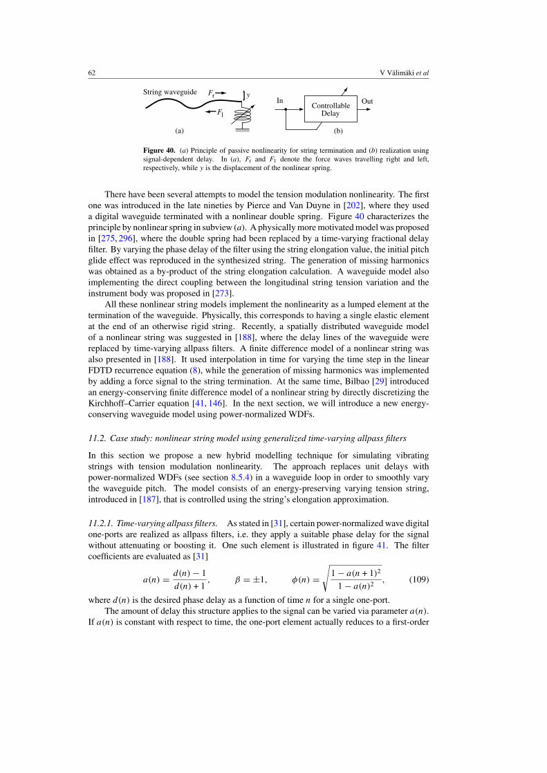
62 V Valimaki et al

ControllableDelay

In Out

(b)

String waveguide Fr

Fl

(a)

y

Figure 40. (a) Principle of passive nonlinearity for string termination and (b) realization usingsignal-dependent delay. In (a), Fr and F1 denote the force waves travelling right and left,respectively, while y is the displacement of the nonlinear spring.

There have been several attempts to model the tension modulation nonlinearity. The firstone was introduced in the late nineties by Pierce and Van Duyne in [202], where they useda digital waveguide terminated with a nonlinear double spring. Figure 40 characterizes theprinciple by nonlinear spring in subview (a). A physically more motivated model was proposedin [275, 296], where the double spring had been replaced by a time-varying fractional delayfilter. By varying the phase delay of the filter using the string elongation value, the initial pitchglide effect was reproduced in the synthesized string. The generation of missing harmonicswas obtained as a by-product of the string elongation calculation. A waveguide model alsoimplementing the direct coupling between the longitudinal string tension variation and theinstrument body was proposed in [273].

All these nonlinear string models implement the nonlinearity as a lumped element at thetermination of the waveguide. Physically, this corresponds to having a single elastic elementat the end of an otherwise rigid string. Recently, a spatially distributed waveguide modelof a nonlinear string was suggested in [188], where the delay lines of the waveguide werereplaced by time-varying allpass filters. A finite difference model of a nonlinear string wasalso presented in [188]. It used interpolation in time for varying the time step in the linearFDTD recurrence equation (8), while the generation of missing harmonics was implementedby adding a force signal to the string termination. At the same time, Bilbao [29] introducedan energy-conserving finite difference model of a nonlinear string by directly discretizing theKirchhoff–Carrier equation [41, 146]. In the next section, we will introduce a new energy-conserving waveguide model using power-normalized WDFs.

11.2. Case study: nonlinear string model using generalized time-varying allpass filters

In this section we propose a new hybrid modelling technique for simulating vibratingstrings with tension modulation nonlinearity. The approach replaces unit delays withpower-normalized WDFs (see section 8.5.4) in a waveguide loop in order to smoothly varythe waveguide pitch. The model consists of an energy-preserving varying tension string,introduced in [187], that is controlled using the string’s elongation approximation.

11.2.1. Time-varying allpass filters. As stated in [31], certain power-normalized wave digitalone-ports are realized as allpass filters, i.e. they apply a suitable phase delay for the signalwithout attenuating or boosting it. One such element is illustrated in figure 41. The filtercoefficients are evaluated as [31]

a(n) = d(n) − 1

d(n) + 1, β = ±1, φ(n) =

√1 − a(n + 1)2

1 − a(n)2, (109)

where d(n) is the desired phase delay as a function of time n for a single one-port.The amount of delay this structure applies to the signal can be varied via parameter a(n).

If a(n) is constant with respect to time, the one-port element actually reduces to a first-order

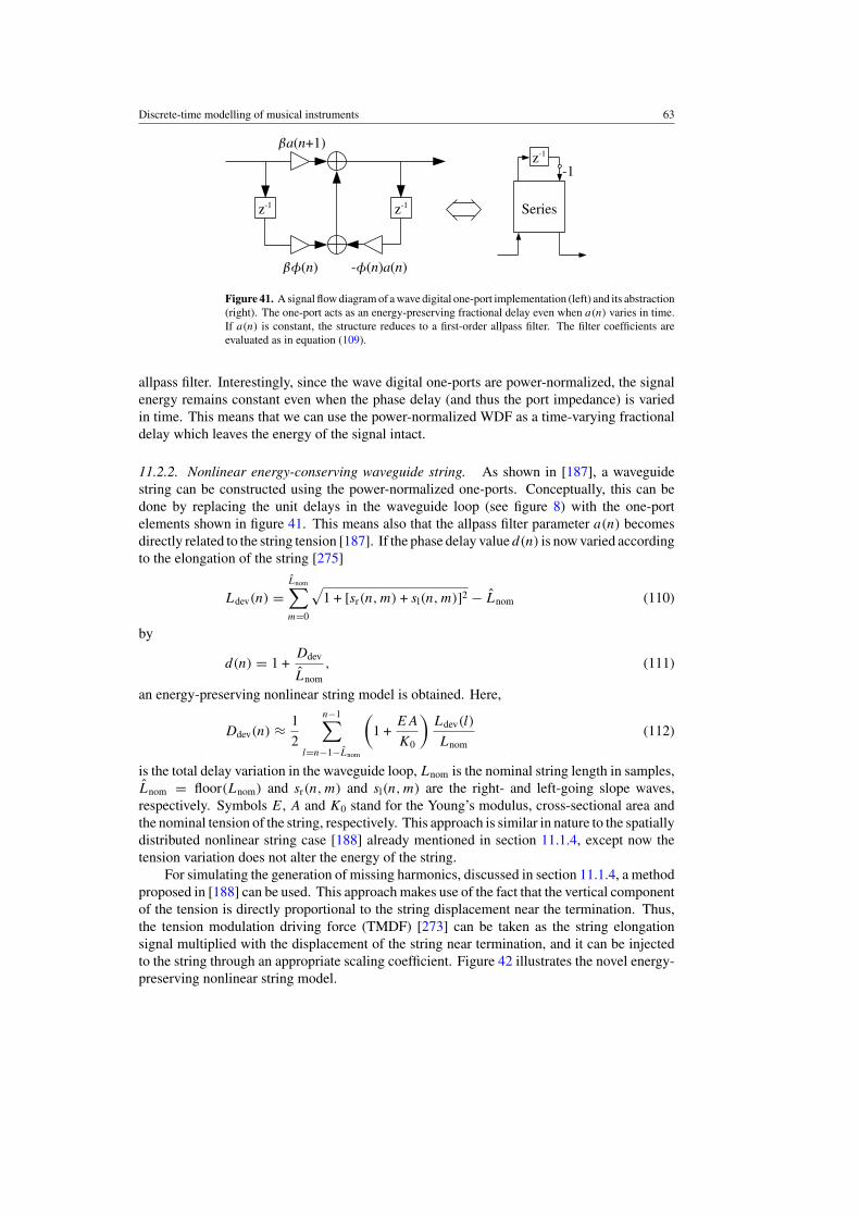
Discrete-time modelling of musical instruments 63

Figure 41. A signal flow diagram of a wave digital one-port implementation (left) and its abstraction(right). The one-port acts as an energy-preserving fractional delay even when a(n) varies in time.If a(n) is constant, the structure reduces to a first-order allpass filter. The filter coefficients areevaluated as in equation (109).

allpass filter. Interestingly, since the wave digital one-ports are power-normalized, the signalenergy remains constant even when the phase delay (and thus the port impedance) is variedin time. This means that we can use the power-normalized WDF as a time-varying fractionaldelay which leaves the energy of the signal intact.

11.2.2. Nonlinear energy-conserving waveguide string. As shown in [187], a waveguidestring can be constructed using the power-normalized one-ports. Conceptually, this can bedone by replacing the unit delays in the waveguide loop (see figure 8) with the one-portelements shown in figure 41. This means also that the allpass filter parameter a(n) becomesdirectly related to the string tension [187]. If the phase delay value d(n) is now varied accordingto the elongation of the string [275]

Ldev(n) =Lnom∑m=0

√1 + [sr(n, m) + sl(n, m)]2 − Lnom (110)

by

d(n) = 1 +Ddev

Lnom

, (111)

an energy-preserving nonlinear string model is obtained. Here,

Ddev(n) ≈ 1

2

n−1∑l=n−1−Lnom

(1 +

EA

K0

)Ldev(l)

Lnom(112)

is the total delay variation in the waveguide loop, Lnom is the nominal string length in samples,Lnom = floor(Lnom) and sr(n, m) and sl(n, m) are the right- and left-going slope waves,respectively. Symbols E, A and K0 stand for the Young’s modulus, cross-sectional area andthe nominal tension of the string, respectively. This approach is similar in nature to the spatiallydistributed nonlinear string case [188] already mentioned in section 11.1.4, except now thetension variation does not alter the energy of the string.

For simulating the generation of missing harmonics, discussed in section 11.1.4, a methodproposed in [188] can be used. This approach makes use of the fact that the vertical componentof the tension is directly proportional to the string displacement near the termination. Thus,the tension modulation driving force (TMDF) [273] can be taken as the string elongationsignal multiplied with the displacement of the string near termination, and it can be injectedto the string through an appropriate scaling coefficient. Figure 42 illustrates the novel energy-preserving nonlinear string model.

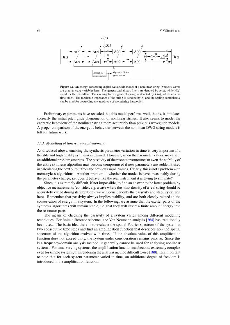
64 V Valimaki et al

Figure 42. An energy-conserving digital waveguide model of a nonlinear string. Velocity wavesare used as wave variables here. The generalized allpass filters are denoted by A(z), while H(z)

stand for the loss filters. The exciting force signal (plucking) is denoted by F(n), where n is thetime index. The mechanic impedance of the string is denoted by Z, and the scaling coefficient α

can be used for controlling the amplitude of the missing harmonics.

Preliminary experiments have revealed that this model performs well, that is, it simulatescorrectly the initial pitch glide phenomenon of nonlinear strings. It also seems to model theenergetic behaviour of the nonlinear string more accurately than previous waveguide models.A proper comparison of the energetic behaviour between the nonlinear DWG string models isleft for future work.

11.3. Modelling of time-varying phenomena

As discussed above, enabling the synthesis parameter variation in time is very important if aflexible and high quality synthesis is desired. However, when the parameter values are varied,an additional problem emerges. The passivity of the resonator structures or even the stability ofthe entire synthesis algorithm may become compromised if new parameters are suddenly usedin calculating the next output from the previous signal values. Clearly, this is not a problem withmemoryless algorithms. Another problem is whether the model behaves reasonably duringthe parameter change, i.e. does it behave like the real instrument it is trying to simulate?

Since it is extremely difficult, if not impossible, to find an answer to the latter problem byobjective measurements (consider, e.g. a case where the mass density of a real string should beaccurately varied during its vibration), we will consider only the passivity and stability criteriahere. Remember that passivity always implies stability, and are both closely related to theconservation of energy in a system. In the following, we assume that the exciter parts of thesynthesis algorithms will remain stable, i.e. that they will insert a finite amount energy intothe resonator parts.

The means of checking the passivity of a system varies among different modellingtechniques. For finite difference schemes, the Von Neumann analysis [264] has traditionallybeen used. The basic idea there is to evaluate the spatial Fourier spectrum of the system attwo consecutive time steps and find an amplification function that describes how the spatialspectrum of the algorithm evolves with time. If the absolute value of this amplificationfunction does not exceed unity, the system under consideration remains passive. Since thisis a frequency-domain analysis method, it generally cannot be used for analysing nonlinearsystems. For time-varying systems, the amplification function can become extremely complexeven for simple systems, thus rendering the analysis method difficult to use [188]. It is importantto note that for each system parameter varied in time, an additional degree of freedom isintroduced in the amplification function.

Discrete-time modelling of musical instruments 65

For models whose implementation essentially consists of filters (modal decomposition,wave and source filter models), time-varying filter analysis methods [53] can be used. Thesemethods are very similar to traditional filter analysis techniques, see, e.g. [176], except that thetime-varying filters possess an additional time variable. As a consequence, the impulse- andfrequency response functions determining the behaviour of the filter become two-dimensional.

For a linear time-varying filter to remain passive, the norm of its generalized impulseresponse cannot exceed unity. In mathematical terms this can be stated as [53]

h(m, n) = 1

a0(n)

[−

K1∑k=1

ak(n)h(m, n − k) +K2∑k=0

bk(n)δ(n − k − m)

]� 1, (113)

where h(m, n) is the output of the system measured at time instant n, when a unity impulseis inserted at the system’s input at time instant m. Coefficients ak(n) and bk(n) correspondto the recursive and non-recursive parts of the system. For K1 > 0, the system is said to bean infinite impulse response (IIR) filter of order K1, while for K1 = 0 it is said to be a finiteimpulse response (FIR) filter of order K2.

By taking the z-transform of equation (113), we have the generalized transfer function ofthe system as

H(z, n) =n∑

m=0

h(m, n)zm−n, (114)

which in the case of an IIR filter consists of a numerator (determined by bk(n)) and adenominator (determined by ak(n)). For ensuring the stability of system, the poles of thefilter, i.e. the roots of the polynomial

∑K1k=0 ak(n), must remain inside the complex unit

circle.For a parallel filter structure, such as a modal synthesis scheme, it suffices to ensure the

stability of the individual resonators. For cascaded filter structures, such as source–filter modelsor commuted waveguides, the transfer function of the whole system, i.e. the convolution ofthe individual filters, must be checked. It must also be noted that since the system is not LTI,the order of the cascaded structure cannot be changed in theory. In practice, however, thecommutation process is often carried out without notable changes in the energetic properties(see, e.g. [250]).

If the system is both nonlinear and time-variant, the energetic analysis becomes even moredifficult. For some modelling techniques, for example WDFs with power-normalized wavevariables (see section 8.5.4), the correct energetic behaviour does not need to be addressed,since the definition of the variables already guarantees passivity. For other systems, ad hocenergy management methods should be used. One obvious approach is the so-called ‘energyprobing’ (see, e.g. [187]), where the signal energy of a system is observed at some locationand compared with pre-calculated limit values. The limit values can be, for example, themaximum and minimum energy levels allowed by physical laws for such a model. When thesignal energy crosses the limit value, the signal must be attenuated or amplified so that it returnsto a suitable energy level. This energy probing can be carried out at several locations in themodel. Needless to say, energy probing can increase the computational load of the synthesisalgorithm substantially.

12. Current trends and further research

Next we look at some current trends in physical modelling. Around the mid-1990s, theresearch reached the point where most Western orchestral instruments could be synthesized

66 V Valimaki et al

based on a physical model [251]. More recently, many papers have been published on themodelling of ethnic and historical musical instruments. These include, for example, the Finnishkantele [82, 130, 186], various lutes [83, 84], the bowed bar [87], ancient Chinese flutes [71],an African flute [72], the Tibetan praying bowl [88, 89], the panpies [69] and the Japanesesho [111, 112]. We have also recently seen applications of physical modelling techniquesto non-musical sound sources [213]. Some examples of these are physical modelling ofbird song [125, 259, 260], various everyday sounds, such as those generated by wind chimes[63,165], footsteps [65] and beach balls [214] and friction models that can be applied in manycases [12].

Another new direction is the subjective evaluation of perceptual features and parameterchanges in physics-based synthesis, see [122, 123, 155, 217]. This line of research providesmusically relevant information on the relation of timbre and the properties of human hearing.These results help in reducing the complexity of synthesis models because details that areinaudible need not be modelled.

The first attempts at audio restoration based on physical models were conductedrecently [85]. While this can be successful for single tones, the practical application of suchmethods for recordings including a mix of several instruments is a challenge for future research.The main problem is high-quality source separation, which is required before this kind ofrestoration process. Sophisticated algorithms have been devised for this task, but, generallyspeaking, separation of a musical signal into individual source signals is still a difficult researchproblem (see, e.g. [147]).

The concept of Structured Audio introduced as part of the MPEG-4 internationalmultimedia standard has opened a new application field for physical models [104, 308]:parametric coding of music, where a program for sound generation of the instruments andcontrol data for playing the instrument are transmitted. The practical use of this idea remainsa dream for the future.

Future work in the field includes, for example, highly accurate modelling of specificmusical instruments. Currently, physics-based synthesis models still lack the excellent soundquality of sample-based digital instruments. A clear example of this defect in quality is seenin digital pianos; the most popular products use a large sample database to reproduce pianotones at all dynamic levels. Fully parametric physical models of the piano have not entered themarket yet, probably because these imitations of the piano are still insufficient for professionalplayers. Difficult subproblems related to this are parameter estimation and control of virtualinstruments. For best sound quality, computational methods that automatically calibrate allthe parameter values of a physical model according to the sound of a good instrument shouldexist. This is very challenging and almost hopeless for some methods, and relatively easyonly for some special cases. The control, or playing, of physical models is another problemarea where general solutions are unavailable. The piano, in fact, is one of the easiest cases,because the player only controls the fundamental frequency (which key) and dynamic level(velocity of key press) of tones. In the cases of string and wind instruments, the control issuerequires clever technical solutions. The control of virtual musical instruments is currently alively research field [61, 67, 116, 121, 136, 137, 161, 191, 315].

An ultimate dream of physical modelling researchers and instrument builders is virtualprototyping of musical instruments. This application will pre-eminently require physicalmodels with excellent precision in the simulation of sound production, as stressed byWoodhouse [319]. A musical instrument designer should have the possibility to modify acomputer model of a musical instrument and then play it to verify that the design is successful.Only after this would the designed instrument be manufactured. Naturally, fine details affectingthe timbre of the instrument should be faithfully simulated, since otherwise this chain of events

Discrete-time modelling of musical instruments 67

would be fruitless. Current research is still far away from this goal. More research work isrequired.

13. Conclusions

Physical modelling of musical instruments has become one of the most active fields of musicalacoustics research. There are six different main approaches to develop a computational modelfor any given instrument. These approaches were briefly overviewed. The digital waveguidemethod, together with its variations, is currently the most popular modelling technique,because it leads to computationally efficient algorithms that enable real-time synthesis ofmany simultaneous voices.

Some current research trends were listed, such as the modelling and synthesis of unusualmusical instruments. It can be predicted that in the near future, the physical modellingtechniques will be applied to numerous everyday sound sources in addition to synthesizingmusical sounds. This research topic has become popular only a few years ago. Non-musicalparametric sounds [66, 215] are of interest because they can be used in human–computerinterfaces, computer games, electronic toys, sound effects for film and animation and virtualreality applications.

Acknowledgments

This work has been funded by the Academy of Finland (Projects 53537, 104934 and105651) and by the Sixth EU Framework Programme for Research and TechnologicalDevelopment (FET-Open Coordination Action IST-2004-03773, ‘Sound to Sense, Sense toSound’). J Pakarinen’s doctoral research is funded by the S3TK Graduate school and TekniikanEdistamissaatio. The authors wish to thank M Tikander for his help in mass–spring networks,K Polonen for his help in hybrid modelling and S Bilbao, C Cadoz, A Chaigne, F Fontana,D T Murphy, S Petrausch, R Rabenstein, X Rodet, A Sarti, S Serafin and J Woodhouse forhelpful discussions and suggestions.

References

[1] Adachi S and Sato M 1995 Time-domain simulation of sound production in the brass instrument J. Acoust.Soc. Am. 97 3850–61

[2] Adrien J M 1989 Dynamic modeling of vibrating structures for sound synthesis, modal synthesis Proc. AudioEngineering Socity 7th Int. Conf.: Audio in Digital Times (Toronto, ON, Canada, May 1989) pp 291–9

[3] Adrien J-M 1991 The missing link: modal synthesis Representations of Musical Signals ed G De Poli et al(Cambridge: MIT Press) pp 269–97

[4] Aird M-L, Laird J and ffitch J 2000 Modelling a drum by interfacing 2-D and 3-D waveguide meshes Proc.Int. Computer Music Conf. (Berlin, Germany, August 2000) pp 82–5

[5] Alles H G 1980 Music synthesis using real time digital techniques Proc. IEEE 68 436–49[6] Anand G V 1969 Large-amplitude damped free vibration of a stretched string J. Acoust. Soc. Am. 45 1089–96[7] Antunes J, Tafasca M and Henrique L 2000 Simulation of the bowed string dynamics 5eme Conference

Française d’Acoustique (Lausanne, Switzerland, 3–7 September 2000)[8] Aramaki M, Bensa J, Daudet L, Guillemain P and Kronland-Martinet R 2001 Resynthesis of coupled piano

string vibrations based on physical modeling J. New Music Res. 30 213–26[9] Arroabarren I and Carlosena A 2004 Vibrato in singing voice: the link between source-filter and sinusoidal

models EURASIP J. Appl. Signal Process. 2004 1007–20 Special issue on model-based sound synthesis[10] Avanzini F 2001 Computational issues in physically-based sound models PhD Thesis Department of Computer

Science and Electronics, University of Padova (Italy)[11] Avanzini F and Rocchesso D 2002 Efficiency, accuracy and stability issues in discrete-time simulations of

single reed wind instruments J. Acoust. Soc. Am. 111 2293–301

68 V Valimaki et al

[12] Avanzini F, Serafin S and Rocchesso D 2002 Modeling interactions between rubbed dry surfaces using an elasto-plastic friction model Proc. COST G6 Conf. on Digital Audio Effects (Hamburg, Germany, September 2002)pp 111–16

[13] Avanzini F and van Walstijn M 2004 Modelling the mechanical response of the reed-mouthpiece-lip system ofa clarinet. Part I. One-dimensional distributed model Acta Acust. united Acust. 90 537–47

[14] Bank B 2000 Physics-based sound synthesis of the piano Master’s Thesis Budapest University of Technologyand Economics, Department of Measurement and Information Systems, Budapest, Hungary

[15] Bank B, Avanzini F, Borin G, De Poli G, Fontana F and Rocchesso D 2003 Physically informed signal-processing methods for piano sound synthesis: a research overview EURASIP J. Appl. Signal Process. 2003941–52 Special Issue on Digital Audio for Multimeda Communications

[16] Bank B and Sujbert L 2005 Generation of longitudinal vibrations in piano strings: from physics to soundsynthesis J. Acoust. Soc. Am. 117 2268–78

[17] Bank B and Valimaki V 2003 Robust loss filter design for digital waveguide synthesis of string tones IEEESignal Process. Lett. 10 18–20

[18] Barjau A and Gibiat V 2003 Delay lines, finite differences and cellular automata: three close but differentschemes for simulating acoustical propagation in 1D systems Acta Acust. united Acust. 88 554–66

[19] Barjau A, Keefe D H and Cardona S 1999 Time-domain simulation of acoustical waveguides with arbitrarilyspaced discontinuities J. Acoust. Soc. Am. 105 1951–64

[20] Beeson M J and Murphy D T 2004 RoomWeaver: A digital waveguide mesh based room acoustics researchtool Proc. COST G6 Conf. Digital Audio Effects (Naples, Italy, October 2004) pp 268–73

[21] Belevitch V 1962 Summary of the history of circuit theory Proc. IRE 50 848–55[22] Bensa J 2003 Analysis and synthesis of piano sounds using physical and signal models PhD Thesis Universite

de la Mediterranee, Marseille, France[23] Bensa J, Bilbao S, Kronland-Martinet R and Smith J O 2003 A power normalized non-linear lossy piano

hammer Proc. Stockholm Music Acoustics Conf. (Stockholm, Sweden, 6–9 August 2003 vol I) pp 365–8[24] Bensa J, Bilbao S, Kronland-Martinet R, Smith J O and Voinier T 2005 Computational modeling of stiff piano

strings using digital waveguides and finite differences Acta Acust. united Acust. 91 289–98[25] Bensa J, Bilbao S, Kronland-Martinet R and Smith J O III 2003 The simulation of piano string vibration: from

physical models to finite difference schemes and digital waveguides J. Acoust. Soc. Am. 114 1095–107[26] Bensa J, Gipouloux O and Kronland-Martinet R 2005 Parameter fitting for piano sound synthesis by physical

modeling J. Acoust. Soc. Am. 118 495–504[27] Bensa J, Jensen K and Kronland-Martinet R 2004 A hybrid resynthesis model for hammer–string interaction

of piano EURASIP J. Appl. Signal Process. 2004 1021–35 Special issue on model-based sound synthesis[28] Berners D and Smith J O 1994 Super-spherical wave simulation in flairing horns Proc. Int. Computer Music

Conf. (Aarhus, Denmark, 1994) pp 112–13[29] Bilbao S 2004 Energy-conserving finite difference schemes for tension-modulated strings IEEE Int. Conf. on

Acoustics Speech and Signal Processing (Montreal, Canada, May 2004) pp 285–8[30] Bilbao S 2004 Wave and Scattering Methods for Numerical Simulation (New York: Wiley)

ISBN: 0-470-87017-6[31] Bilbao S 2005 Time-varying generalizations of all-pass filters IEEE Signal Process. Lett. 12 376–9[32] Bisnovatyi I 2000 Flexible software framework for modal synthesis Proc. COST G-6 Conf. on Digital Audio

Effects (Verona, Italy, December 2000) pp 109–14[33] Borin G, De Poli G and Rocchesso D 2000 Elimination of delay-free loops in discrete-time models of nonlinear

acoustic systems IEEE Trans. Speech Audio Process. 8 597–605[34] Boutillon X 1988 Model for piano hammers: experimental determination and digital simulation J. Acoust. Soc.

Am. 83 746–54[35] Brandt E 2001 Hard sync without aliasing Proc. Int. Computer Music Conf. (Havana, Cuba, September 2001)

pp 365–8[36] Cadoz C 2002 The physical model as a metaphor for musical creation ‘pico..TERA’, a piece entirely generated

by physical model Proc. Int. Computer Music Conf. (Gothenburg, Sweden, 2002) pp 305–12[37] Cadoz C, Florens J-L and Gubian S 2001 Bowed string synthesis with force feedback gestural interaction Proc.

Int. Comput. Music Conf. (Havana, Cuba, 2001)[38] Cadoz C, Luciani A and Florens J-L 1983 Responsive input devices and sound synthesis by simulation of

instrumental mechanisms: the CORDIS system Comput. Music J. 8 60–73[39] Cadoz C, Luciani A and Florens J-L 2003 Artistic creation and computer interactive multisensory simulation

force feedback gesture transducers NIME: Proc. Conf. on New Interfaces for Musical Expression (Montreal,Canada, May 2003) pp 235–46

[40] Campbell M 2004 Brass instruments as we know them today Acta Acust. united Acust. 4 600–10

Discrete-time modelling of musical instruments 69

[41] Carrier G F 1945 On the nonlinear vibration of an elastic string Q. Appl. Math. 3 157–65[42] Castagne N and Cadoz C 2002 Creating music by means of ‘physical thinking’: the musician oriented

Genesis environment Proc. COST G6 Conf. on Digital Audio Effects (Hamburg, Germany, September2002) pp 169–74

[43] Chadabe J 1997 Electric Sound: the Past and Promise of Electronic Music (New Jersey: Prentice-Hall)[44] Chafe C 1995 Adding vortex noise to wind instrument physical models Proc. Int. Computer Music Conf. (Banff,

Canada, September 1995) pp 57–60[45] Chaigne A 1992 On the use of finite differences for musical synthesis. Application to plucked stringed

instruments J. Acoust. 5 181–211[46] Chaigne A and Askenfelt A 1994 Numerical simulations of piano strings. I. A physical model for a struck

string using finite difference methods J. Acoust. Soc. Am. 95 1112–18[47] Chaigne A and Askenfelt A 1994 Numerical simulations of piano strings. II. Comparisons with measurements

and systematic exploration of some hammer–string parameters J. Acoust. Soc. Am. 95 1631–40[48] Chaigne A and Doutaut V 1997 Numerical simulations of xylophones. I. Time-domain modeling of the vibrating

bars J. Acoust. Soc. Am. 101 539–57[49] Chaigne A, Fontaine M, Thomas O, Ferre M and Touze C 2002 Vibrations of shallow spherical shells and

gongs: a comparative study Proc. Forum Acusticum (Sevilla, 2002)[50] Chaigne A and Lambourg C 2001 Time-domain simulation of damped impacted plates. Part I. Theory and

experiments J. Acoust. Soc. Am. 109 1422–32[51] Chaigne A, Touze C and Thomas O 2001 Nonlinear axisymmetric vibrations of gongs Proc. Int. Symp. on

Musical Acoustics (Perugia, 2001)[52] Chaigne A, Touze C and Thomas O 2004 Mechanical models of musical instruments and sound synthesis: the

case of gongs and cymbals Proc. Int. Symp. on Musical Acoustics (Nara, Japan, 2004)[53] Cherniakov M 2003 An Introduction to Parametric Digital Filters and Oscillators (New York: Wiley) 2003

ISBN: 047085104X[54] Chowning J 1973 The synthesis of complex audio spectra by means of frequency modulation J. Audio Eng.

Soc. 21 526–34[55] Coltman J 1992 Time-domain simulation of the flute J. Acoust. Soc. Am. 92 69–73[56] Comajuncosas J M 2000 Physical models of strings and plates using a simplified mass-spring method The

Csound Book ed R Boulanger (Cambridge: MIT Press) chapter 20 (CD-ROM)[57] Conklin H A 1996 Design and tone in the mechanoacoustic piano. Part III. Piano strings and scale design

J. Acoust. Soc. Am. 100 1286–98[58] Conklin H A 1999 Generation of partials due to nonlinear mixing in a stringed instrument J. Acoust. Soc. Am.

105 536–45[59] Cook P 1991 Identification of control parameters in an articulatory vocal tract model, with applications to the

synthesis of singing PhD Thesis CCRMA, Stanford University[60] Cook P 1996 Singing voice synthesis: history, current work and future directions Comput. Music J. 20[61] Cook P R 1992 A meta-wind-instrument physical model, and a meta-controller for real-time performance

control Proc. Int. Computer Music Conf. (San Jose, California, October 1992) pp 273–6[62] Cook P R 1995 Integration of physical modeling for synthesis and animation Proc. Int. Computer Music Conf.

(Banff, Canada, September 1995) pp 525–8[63] Cook P R 1997 Physically informed sonic modeling (PhISM): synthesis of percussive sounds Comput. Music

J. 21 38–49[64] Cook P R 2001 SPASM: a real-time vocal tract physical model editor/controller and singer: the companion

software synthesis system Comput. Music J. 17 30–44[65] Cook P R 2002 Modeling Bill’s gait: analysis and parametric synthesis of walking sounds Proc. AES 22nd Int.

Conf. on Virtual, Synthetic and Entertainment Audio (Espoo, Finland, June 2002) pp 73–8[66] Cook P R 2002 Real Sound Synthesis for Interactive Applications (Wellesley: Peters A K) 2002 ISBN 1-56881-

168-3[67] Cook P R 2004 Remutualizing the musical instrument: co-design of synthesis algorithms and controllers J. New

Music Res. 33 315–20[68] Cremer L 1983 The Physics of the Violin (Cambridge: MIT Press)[69] Czyzewski A and Kostek B 2003 Waveguide modelling of the panpipes Proc. Stockholm Music Acoustics Conf.

(Stockholm, Sweden, August 2003 vol 1) pp 259–62[70] de Bruin G and van Walstijn M 1995 Physical models of wind instruments: a generalized excitation coupled

with a modular simulation platform J. New Music Res. 24 148–63[71] de la Cuadra P, Smyth T, Chafe C and Baoqiang H 2001 Waveguide simulation of neolithic Chinese flutes Proc.

Int. Symp. on Musical Acoustics (Perugia, Italy, September 2001) pp 181–4

70 V Valimaki et al

[72] de la Cuadra P, Vergez C and Causse R 2002 Use of physical-model synthesis for developing experimentaltechniques in ethnomusicology—the case of the ouldeme flute Proc. Int. Computer Music Conf.(Gothenburg, Sweden, 2002) pp 53–6

[73] De Poli G and Rocchesso D 1998 Physically based sound modelling Organised Sound 3 61–76[74] Depalle P and Tassart S 1995 State space sound synthesis and a state space synthesiser builder Proc. Int.

Computer Music Conf. (Banff, Canada, September 1995) pp 88–95[75] Derveaux G, Chaigne A, Joly P and Bécache E 2003 Time-domain simulation of a guitar: model and method

J. Acoust. Soc. Am. 114 3368–83[76] Dietz P H and Amir N 1995 Synthesis of trumpet tones by physical modeling Proc. Int. Symp. on Musical

Acoustics (Dourdan, France, 1995) pp 472–7[77] Ducasse E 2002 An alternative to the traveling-wave approach for use in two-port descriptions of acoustic

bores J. Acoust. Soc. Am. 112 3031–41[78] Eckel G, Iovino F and Causse R 1995 Sound synthesis by physical modelling with Modalys Proc. Int. Symp.

on Musical Acoustics (Dourdan, France, July 1995) pp 479–82[79] Erkut C 2001 Model order selection techniques for the loop filter design of virtual string instruments Proc.

5th World Multi-Conf. on Systems, Cybernetics and Informatics (Orlando, FL, USA, July 2001 vol 10)pp 529–34

[80] Erkut C and Karjalainen M 2002 Finite difference method vs. digital waveguide method in string instrumentmodeling and synthesis Proc. Int. Symp. on Musical Acoustics (Mexico City, Mexico, December 2002)CD-ROM proceedings

[81] Erkut C and Karjalainen M 2002 Virtual strings based on a 1-D FDTD waveguide model: stability, losses, andtravelling waves Proc. AES 22nd Int. Conf. ( Espoo, Finland, June 2002) pp 317–23

[82] Erkut C, Karjalainen M, Huang P and Valimaki V 2002 Acoustical analysis and model-based sound synthesisof the kantele J. Acoust. Soc. Am. 112 1681–91

[83] Erkut C, Laurson M, Kuuskankare M and Valimaki V 2001 Model-based synthesis of the ud and the Renaissancelute Proc. Int. Computer Music Conf. (Havana, Cuba, September 2001) pp 119–22

[84] Erkut C and Valimaki V 2000 Model-based sound synthesis of tanbur, a Turkish long-necked lute IEEE Int.Conf. on Acoustics Speech and Signal Processing (Istanbul, Turkey, June 2000) pp 769–772 Available onlineat http://lib.tkk.fi/Diss/2002/isbn9512261901/

[85] Esquef P, Valimaki V and Karjalainen M 2002 Restoration and enhancement of solo guitar recordings basedon sound source modeling J. Audio Eng. Soc. 50 227–36

[86] Essl G 2002 Physical wave propagation modeling for real-time synthesis of natural sounds PhD Thesis PrincetonUniversity, Department of Computer Science, Princeton, NJ

[87] Essl G and Cook P R 2000 Measurements and efficient simulations of bowed bars J. Acoust. Soc. Am. 108379–88

[88] Essl G and Cook P R 2002 Banded waveguides on circular topologies and of beating modes: Tibetan singingbowls and glass harmonicas Proc. Int. Computer Music Conf. (Gothenburg, Sweden, 2002) InternationalComputer Music Association pp 49–52

[89] Essl G, Serafin S, Cook P R and Smith J O 2004 Musical applications of banded waveguides Comput. MusicJ. 28 51–63

[90] Essl G, Serafin S, Cook P R and Smith J O 2004 Theory of banded waveguides Comput. Music J.28 37–50

[91] Fabre B and Hirschberg A 2000 Physical modeling of flue instruments: a review of lumped models Acta Acust.united Acust. 86 599–610

[92] Fant G 1970 Acoustic Theory of Speech Production (The Hague: Mouton)[93] Fettweis A 1971 Digital filters related to classical structures AEU: Archive fur Elektronik und

Ubertragungstechnik 25 78–89[94] Fettweis A 1986 Wave digital filters: theory and practice Proc. IEEE 74 270–327[95] Flanagan J 1972 Speech Analysis, Synthesis and Perception (Berlin: Springer)[96] Fletcher N H and Rossing T D 1991 The Physics of Musical Instruments (New York: Springer)[97] Fletcher N H 1999 The nonlinear physics of musical instruments Rep. Prog. Phys. 62 723–64[98] Florens J-L and Cadoz C 1991 The physical model: modeling and simulating the instrumental universe

Representations of Musical Signals ed G De Poli et al (Cambridge: MIT Press) pp 227–68[99] Fontana F 2003 Computation of linear filter networks containing delay-free loops, with an application to the

waveguide mesh IEEE Trans. Speech Audio Process. 11 774–82[100] Fontana F and Rocchesso D 1998 Physical modeling of membranes for percussion instruments Acta Acust.

united Acust. 84 529–42[101] Fontana F and Rocchesso D 2000 Online correction of dispersion error in 2D waveguide meshes Proc. Int.

Computer Music Conf. (Berlin, Germany, August 2000) pp 78–81

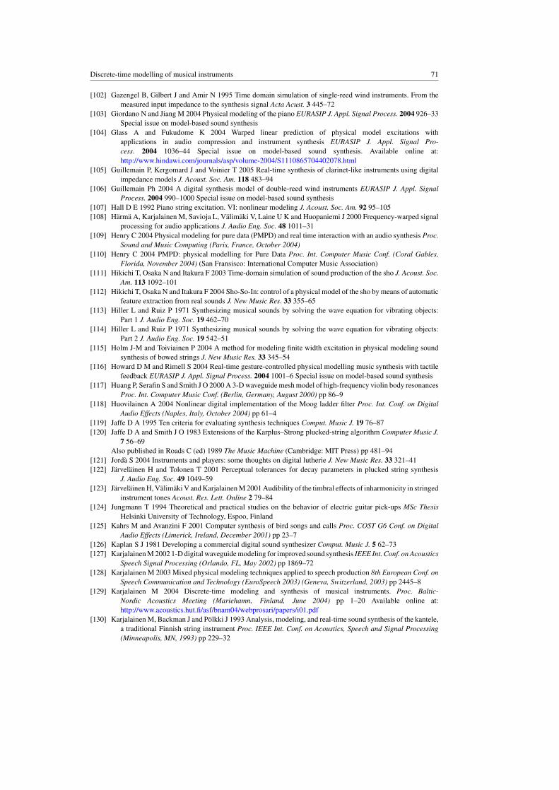
Discrete-time modelling of musical instruments 71

[102] Gazengel B, Gilbert J and Amir N 1995 Time domain simulation of single-reed wind instruments. From themeasured input impedance to the synthesis signal Acta Acust. 3 445–72

[103] Giordano N and Jiang M 2004 Physical modeling of the piano EURASIP J. Appl. Signal Process. 2004 926–33Special issue on model-based sound synthesis

[104] Glass A and Fukudome K 2004 Warped linear prediction of physical model excitations withapplications in audio compression and instrument synthesis EURASIP J. Appl. Signal Pro-cess. 2004 1036–44 Special issue on model-based sound synthesis. Available online at:http://www.hindawi.com/journals/asp/volume-2004/S1110865704402078.html

[105] Guillemain P, Kergomard J and Voinier T 2005 Real-time synthesis of clarinet-like instruments using digitalimpedance models J. Acoust. Soc. Am. 118 483–94

[106] Guillemain Ph 2004 A digital synthesis model of double-reed wind instruments EURASIP J. Appl. SignalProcess. 2004 990–1000 Special issue on model-based sound synthesis

[107] Hall D E 1992 Piano string excitation. VI: nonlinear modeling J. Acoust. Soc. Am. 92 95–105[108] Harma A, Karjalainen M, Savioja L, Valimaki V, Laine U K and Huopaniemi J 2000 Frequency-warped signal

processing for audio applications J. Audio Eng. Soc. 48 1011–31[109] Henry C 2004 Physical modeling for pure data (PMPD) and real time interaction with an audio synthesis Proc.

Sound and Music Computing (Paris, France, October 2004)[110] Henry C 2004 PMPD: physical modelling for Pure Data Proc. Int. Computer Music Conf. (Coral Gables,

Florida, November 2004) (San Fransisco: International Computer Music Association)[111] Hikichi T, Osaka N and Itakura F 2003 Time-domain simulation of sound production of the sho J. Acoust. Soc.

Am. 113 1092–101[112] Hikichi T, Osaka N and Itakura F 2004 Sho-So-In: control of a physical model of the sho by means of automatic

feature extraction from real sounds J. New Music Res. 33 355–65[113] Hiller L and Ruiz P 1971 Synthesizing musical sounds by solving the wave equation for vibrating objects:

Part 1 J. Audio Eng. Soc. 19 462–70[114] Hiller L and Ruiz P 1971 Synthesizing musical sounds by solving the wave equation for vibrating objects:

Part 2 J. Audio Eng. Soc. 19 542–51[115] Holm J-M and Toiviainen P 2004 A method for modeling finite width excitation in physical modeling sound

synthesis of bowed strings J. New Music Res. 33 345–54[116] Howard D M and Rimell S 2004 Real-time gesture-controlled physical modelling music synthesis with tactile

feedback EURASIP J. Appl. Signal Process. 2004 1001–6 Special issue on model-based sound synthesis[117] Huang P, Serafin S and Smith J O 2000 A 3-D waveguide mesh model of high-frequency violin body resonances

Proc. Int. Computer Music Conf. (Berlin, Germany, August 2000) pp 86–9[118] Huovilainen A 2004 Nonlinear digital implementation of the Moog ladder filter Proc. Int. Conf. on Digital

Audio Effects (Naples, Italy, October 2004) pp 61–4[119] Jaffe D A 1995 Ten criteria for evaluating synthesis techniques Comput. Music J. 19 76–87[120] Jaffe D A and Smith J O 1983 Extensions of the Karplus–Strong plucked-string algorithm Computer Music J.

7 56–69Also published in Roads C (ed) 1989 The Music Machine (Cambridge: MIT Press) pp 481–94

[121] Jorda S 2004 Instruments and players: some thoughts on digital lutherie J. New Music Res. 33 321–41[122] Jarvelainen H and Tolonen T 2001 Perceptual tolerances for decay parameters in plucked string synthesis

J. Audio Eng. Soc. 49 1049–59[123] Jarvelainen H, Valimaki V and Karjalainen M 2001 Audibility of the timbral effects of inharmonicity in stringed

instrument tones Acoust. Res. Lett. Online 2 79–84[124] Jungmann T 1994 Theoretical and practical studies on the behavior of electric guitar pick-ups MSc Thesis

Helsinki University of Technology, Espoo, Finland[125] Kahrs M and Avanzini F 2001 Computer synthesis of bird songs and calls Proc. COST G6 Conf. on Digital

Audio Effects (Limerick, Ireland, December 2001) pp 23–7[126] Kaplan S J 1981 Developing a commercial digital sound synthesizer Comput. Music J. 5 62–73[127] Karjalainen M 2002 1-D digital waveguide modeling for improved sound synthesis IEEE Int. Conf. on Acoustics

Speech Signal Processing (Orlando, FL, May 2002) pp 1869–72[128] Karjalainen M 2003 Mixed physical modeling techniques applied to speech production 8th European Conf. on

Speech Communication and Technology (EuroSpeech 2003) (Geneva, Switzerland, 2003) pp 2445–8[129] Karjalainen M 2004 Discrete-time modeling and synthesis of musical instruments. Proc. Baltic-

Nordic Acoustics Meeting (Mariehamn, Finland, June 2004) pp 1–20 Available online at:http://www.acoustics.hut.fi/asf/bnam04/webprosari/papers/i01.pdf

[130] Karjalainen M, Backman J and Polkki J 1993 Analysis, modeling, and real-time sound synthesis of the kantele,a traditional Finnish string instrument Proc. IEEE Int. Conf. on Acoustics, Speech and Signal Processing(Minneapolis, MN, 1993) pp 229–32

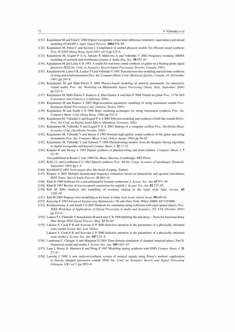
72 V Valimaki et al

[131] Karjalainen M and Erkut C 2004 Digital waveguides versus finite difference structures: equivalence and mixedmodeling EURASIP J. Appl. Signal Process. 2004 978–89

[132] Karjalainen M, Erkut C and Savioja L Compilation of unified physical models for efficient sound synthesisProc. ICASSP (Hong Kong, April 2003 vol 5) pp 433–6

[133] Karjalainen M, Esquef P A A, Antsalo P, Makivirta A and Valimaki V 2002 Frequency-zooming ARMAmodeling of resonant and reverberant systems J. Audio Eng. Soc. 50 953–67

[134] Karjalainen M and Laine U K 1991 A model for real-time sound synthesis of guitar on a floating-point signalprocessor IEEE Int. Conf. on Acoustics Speech Signal Processing (Toronto, Canada, 1991)

[135] Karjalainen M, Laine U K, Laakso T I and Valimaki V 1991 Transmission-line modeling and real-time synthesisof string and wind instruments Proc. Int. Computer Music Conf. (Montreal, Quebec, Canada, 16–20 October1991) pp 293–6

[136] Karjalainen M and Maki-Patola T 2004 Physics-based modeling of musical instruments for interactivevirtual reality Proc. Int. Workshop on Multimedia Signal Processing (Siena, Italy, September 2004)pp 223–6

[137] Karjalainen M, Maki-Patola T, Kanerva A, Huovilainen A and Janis P 2004 Virtual air guitar Proc. 117th AESConvention (San Francisco, California, 2004)

[138] Karjalainen M and Paatero T 2005 High-resolution parametric modeling of string instrument sounds Proc.European Signal Processing Conf. (Antalya, Turkey, 2005)

[139] Karjalainen M and Smith J O 1996 Body modeling techniques for string instrument synthesis Proc. Int.Computer Music Conf. (Hong Kong, 1996) pp 232–9

[140] Karjalainen M, Valimaki V and Esquef P A A 2002 Efficient modeling and synthesis of bell-like sounds DAFx:Proc. Int. Conf. on Digital Audio Effects (Hamburg, Germany, 2002)

[141] Karjalainen M, Valimaki V and Esquef P A A 2003 Making of a computer carillon Proc. Stockholm MusicAcoustics Conf. (Stockholm, Sweden, 2003)

[142] Karjalainen M, Valimaki V and Janosy Z 1993 Towards high-quality sound synthesis of the guitar and stringinstruments Proc. Int. Computer Music Conf. (Tokyo, Japan, 1993) pp 56–63

[143] Karjalainen M, Valimaki V and Tolonen T 1998 Plucked-string models: from the Karplus–Strong algorithmto digital waveguides and beyond Comput. Music J. 22 17–32

[144] Karplus K and Strong A 1983 Digital synthesis of plucked-string and drum timbres. Computer Music J. 743–55

Also published in Roads C (ed) 1989 The Music Machine (Cambridge: MIT Press)[145] Kelly J L and Lochbaum C C 1962 Speech synthesis Proc. 4th Int. Congr. Acoustics (Copenhagen, Denmark,

September 1962) pp 1–4[146] Kirchhoff G 1883 Vorlesungen uber Mechanik (Leipzig: Tauber)[147] Klapuri A 2003 Multiple fundamental frequency estimation based on harmonicity and spectral smoothness

IEEE Trans. Speech Audio Process. 11 804–16[148] Klatt D 1980 Software for a cascade/parallel formant synthesizer J. Acoust. Soc. Am. 67 971–95[149] Klatt D 1987 Review of text-to-speech conversion for english J. Acoust. Soc. Am. 82 737–93[150] Kob M 2004 Analysis and modelling of overtone singing in the sygyt style Appl. Acoust. 65

1249–59[151] Kob M 2004 Singing voice modelling as we know it today Acta Acust. united Acust. 90 649–61[152] Kreyszig E 1992 Advanced Engineering Mathematics 7th edn (New York: Wiley) ISBN: 0471553808[153] Krishnaswamy A and Smith J O 2003 Methods for simulating string collisions with rigid spatial objects Proc.

IEEE Workshop of Applications of Signal Processing to Audio and Acoustics, NY, USA (October 2003)pp 233–6

[154] Laakso T I, Valimaki V, Karjalainen M and Laine U K 1996 Splitting the unit delay—Tools for fractional delayfilter design IEEE Signal Process. Mag. 13 30–60

[155] Lakatos S, Cook P R and Scavone G P 2000 Selective attention to the parameters of a physically informedsonic model Acoust. Res. Lett. Online

Lakatos S, Cook P R and Scavone G P 2000 Selective attention to the parameters of a physically informedsonic model J. Acoust. Soc. Am. 107 L31–6

[156] Lambourg C, Chaigne A and Matignon D 2001 Time-domain simulation of damped impacted plates. Part II.Numerical model and results J. Acoust. Soc. Am. 109 1433–47

[157] Lane J, Hoory D, Martinez E and Wang P 1997 Modeling analog synthesis with DSPs Comput. Music J. 2123–41

[158] Laroche J 1989 A new analysis/synthesis system of musical signals using Prony’s method—applicationto heavily damped percussive sounds IEEE Int. Conf. on Acoustics Speech and Signal Processing(Glasgow, UK) vol 3, pp 2053–6

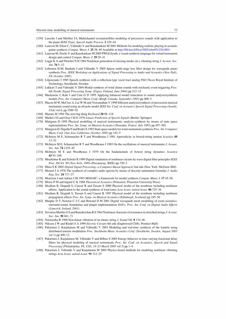
Discrete-time modelling of musical instruments 73

[159] Laroche J and Meillier J-L Multichannel excitation/filter modeling of percussive sounds with application tothe piano IEEE Trans. Speech Audio Process. 2 329–44

[160] Laurson M, Erkut C, Valimaki V and Kuuskankare M 2001 Methods for modeling realistic playing in acousticguitar synthesis Comput. Music J. 25 38–49 Available at http://lib.hut.fi/Diss/2002/isbn9512261901/

[161] Laurson M, Norilo V and Kuuskankare M 2005 PWGLSynth: a visual synthesis language for virtual instrumentdesign and control Comput. Music J. 29 29–41

[162] Legge K A and Fletcher N H 1984 Nonlinear generation of missing modes on a vibrating string J. Acoust. Soc.Am. 76 5–12

[163] Lehtonen H-M, Rauhala J and Valimaki V 2005 Sparse multi-stage loss filter design for waveguide pianosynthesis Proc. IEEE Workshop on Applications of Signal Processing to Audio and Acoustics (New Paltz,NY, October 2005)

[164] Liljencrantz J 1985 Speech synthesis with a reflection-type vocal tract analog PhD Thesis Royal Institute ofTechnology, Stockholm, Sweden

[165] Lukkari T and Valimaki V 2004 Modal synthesis of wind chime sounds with stochastic event triggering Proc.6th Nordic Signal Processing Symp. (Espoo, Finland, June 2004) pp 212–15

[166] Mackenzie J, Kale I and Cain G D 1995 Applying balanced model truncation to sound analysis/synthesismodels Proc. Int. Computer Music Conf. (Banff, Canada, September 1995) pp 400–3

[167] Macon M W, McCree A, Lai W M and Viswanathan V 1998 Efficient analysis/synthesis of percussion musicalinstrument sound using an all-pole model IEEE Int. Conf. on Acoustics Speech Signal Processing (Seattle,USA) vol 6, pp 3589–92

[168] Marans M 1994 The next big thing Keyboard 20 98–118[169] Markel J D and Gray J H G 1976 Linear Prediction of Speech Signals (Berlin: Springer)[170] Matignon D 1995 Physical modelling of musical instruments: analysis-synthesis by means of state space

representations Proc. Int. Symp. on Musical Acoustics (Dourdan, France, July 1995) pp 497–502[171] Matignon D, Depalle P and Rodet X 1992 State space models for wind-instrument synthesis Proc. Int. Computer

Music Conf. (San Jose California, October 1992) pp 142–5[172] McIntyre M E, Schumacher R T and Woodhouse J 1981 Aperiodicity in bowed-string motion Acustica 49

13–32[173] McIntyre M E, Schumacher R T and Woodhouse J 1983 On the oscillations of musical instruments J. Acoust.

Soc. Am. 74 1325–45[174] McIntyre M E and Woodhouse J 1979 On the fundamentals of bowed string dynamics Acustica

43 93–108[175] Meerkotter K and Scholtz R 1989 Digital simulation of nonlinear circuits by wave digital filter principles IEEE

Proc. ISCAS ’89 (New York, 1989) (Piscataway: IEEE) pp 720–3[176] Mitra S K 2002 Digital Signal Processing: a Computer-Based Approach 2nd edn (New York: McGraw-Hill)[177] Moorer J A 1976 The synthesis of complex audio spectra by means of discrete summation formulae J. Audio

Eng. Soc. 24 717–27[178] Morrison J and Adrien J M 1993 MOSAIC: a framework for modal synthesis Comput. Music J. 17 45–56[179] Morse P M and Ingard U K 1968 Theoretical Acoustics (Princeton: Princeton University Press)[180] Msallam R, Dequidt S, Causse R and Tassart S 2000 Physical model of the trombone including nonlinear

effects. Application to the sound synthesis of loud tones Acta Acust. united Acust. 86 725–36[181] Msallam R, Dequidt S, Tassart S and Causse R 1997 Physical model of the trombone including nonlinear

propagation effects Proc. Int. Symp. on Musical Acoustics (Edinburgh, Scotland) pp 245–50[182] Murphy D T, Newton C J C and Howard D M 2001 Digital waveguide mesh modelling of room acoustics:

surround-sound, boundaries and plugin implementation DAFx: Proc. Int. Conf. on Digital Audio Effects(Limerick, Ireland, 2001)

[183] Srivinisa Murthy G S and Ramakrishna B S 1964 Nonlinear character of resonance in stretched strings J. Acoust.Soc. Am. 38 461–71

[184] Narasimha R 1968 Non-linear vibration of an elastic string J. Sound Vib. 8 134–46[185] Nilsson J W and Riedel S A 1999 Electric Circuits 6th edn (Englewood Cliffs: Prentice-Hall)[186] Pakarinen J, Karjalainen M and Valimaki V 2003 Modeling and real-time synthesis of the kantele using

distributed tension modulation Proc. Stockholm Music Acoustics Conf. (Stockholm, Sweden, August 2003vol 1) pp 409–12

[187] Pakarinen J, Karjalainen M, Valimaki V and Bilbao S 2005 Energy behavior in time-varying fractional delayfilters for physical modeling of musical instruments Proc. Int. Conf. on Acoustics, Speech and SignalProcessing (Philadelphia, PA, USA, 19–23 March 2005 vol 3) pp 1–4

[188] Pakarinen J, Valimaki V and Karjalainen M 2005 Physics-based methods for modeling nonlinear vibratingstrings Acta Acust. united Acust. 91 312–25

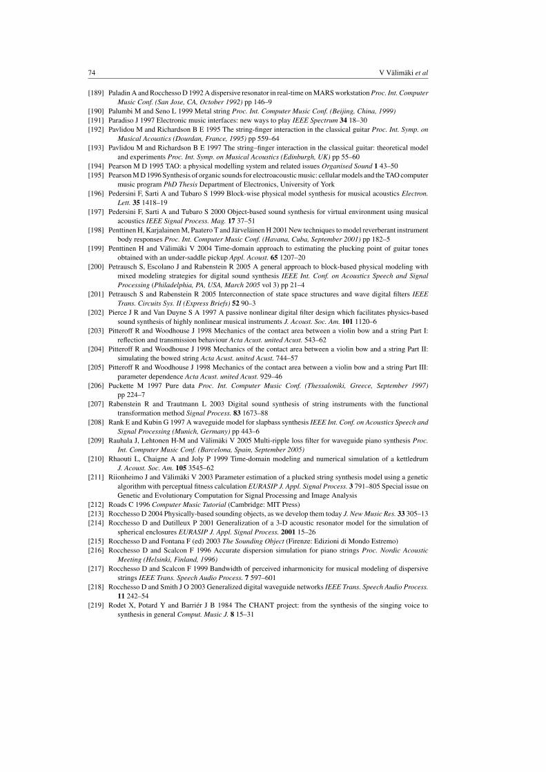
74 V Valimaki et al

[189] Paladin A and Rocchesso D 1992 A dispersive resonator in real-time on MARS workstation Proc. Int. ComputerMusic Conf. (San Jose, CA, October 1992) pp 146–9

[190] Palumbi M and Seno L 1999 Metal string Proc. Int. Computer Music Conf. (Beijing, China, 1999)[191] Paradiso J 1997 Electronic music interfaces: new ways to play IEEE Spectrum 34 18–30[192] Pavlidou M and Richardson B E 1995 The string-finger interaction in the classical guitar Proc. Int. Symp. on

Musical Acoustics (Dourdan, France, 1995) pp 559–64[193] Pavlidou M and Richardson B E 1997 The string–finger interaction in the classical guitar: theoretical model

and experiments Proc. Int. Symp. on Musical Acoustics (Edinburgh, UK) pp 55–60[194] Pearson M D 1995 TAO: a physical modelling system and related issues Organised Sound 1 43–50[195] Pearson M D 1996 Synthesis of organic sounds for electroacoustic music: cellular models and the TAO computer

music program PhD Thesis Department of Electronics, University of York[196] Pedersini F, Sarti A and Tubaro S 1999 Block-wise physical model synthesis for musical acoustics Electron.

Lett. 35 1418–19[197] Pedersini F, Sarti A and Tubaro S 2000 Object-based sound synthesis for virtual environment using musical

acoustics IEEE Signal Process. Mag. 17 37–51[198] Penttinen H, Karjalainen M, Paatero T and Jarvelainen H 2001 New techniques to model reverberant instrument

body responses Proc. Int. Computer Music Conf. (Havana, Cuba, September 2001) pp 182–5[199] Penttinen H and Valimaki V 2004 Time-domain approach to estimating the plucking point of guitar tones

obtained with an under-saddle pickup Appl. Acoust. 65 1207–20[200] Petrausch S, Escolano J and Rabenstein R 2005 A general approach to block-based physical modeling with

mixed modeling strategies for digital sound synthesis IEEE Int. Conf. on Acoustics Speech and SignalProcessing (Philadelphia, PA, USA, March 2005 vol 3) pp 21–4

[201] Petrausch S and Rabenstein R 2005 Interconnection of state space structures and wave digital filters IEEETrans. Circuits Sys. II (Express Briefs) 52 90–3

[202] Pierce J R and Van Duyne S A 1997 A passive nonlinear digital filter design which facilitates physics-basedsound synthesis of highly nonlinear musical instruments J. Acoust. Soc. Am. 101 1120–6

[203] Pitteroff R and Woodhouse J 1998 Mechanics of the contact area between a violin bow and a string Part I:reflection and transmission behaviour Acta Acust. united Acust. 543–62

[204] Pitteroff R and Woodhouse J 1998 Mechanics of the contact area between a violin bow and a string Part II:simulating the bowed string Acta Acust. united Acust. 744–57

[205] Pitteroff R and Woodhouse J 1998 Mechanics of the contact area between a violin bow and a string Part III:parameter dependence Acta Acust. united Acust. 929–46

[206] Puckette M 1997 Pure data Proc. Int. Computer Music Conf. (Thessaloniki, Greece, September 1997)pp 224–7

[207] Rabenstein R and Trautmann L 2003 Digital sound synthesis of string instruments with the functionaltransformation method Signal Process. 83 1673–88

[208] Rank E and Kubin G 1997 A waveguide model for slapbass synthesis IEEE Int. Conf. on Acoustics Speech andSignal Processing (Munich, Germany) pp 443–6

[209] Rauhala J, Lehtonen H-M and Valimaki V 2005 Multi-ripple loss filter for waveguide piano synthesis Proc.Int. Computer Music Conf. (Barcelona, Spain, September 2005)

[210] Rhaouti L, Chaigne A and Joly P 1999 Time-domain modeling and numerical simulation of a kettledrumJ. Acoust. Soc. Am. 105 3545–62

[211] Riionheimo J and Valimaki V 2003 Parameter estimation of a plucked string synthesis model using a geneticalgorithm with perceptual fitness calculation EURASIP J. Appl. Signal Process. 3 791–805 Special issue onGenetic and Evolutionary Computation for Signal Processing and Image Analysis

[212] Roads C 1996 Computer Music Tutorial (Cambridge: MIT Press)[213] Rocchesso D 2004 Physically-based sounding objects, as we develop them today J. New Music Res. 33 305–13[214] Rocchesso D and Dutilleux P 2001 Generalization of a 3-D acoustic resonator model for the simulation of

spherical enclosures EURASIP J. Appl. Signal Process. 2001 15–26[215] Rocchesso D and Fontana F (ed) 2003 The Sounding Object (Firenze: Edizioni di Mondo Estremo)[216] Rocchesso D and Scalcon F 1996 Accurate dispersion simulation for piano strings Proc. Nordic Acoustic

Meeting (Helsinki, Finland, 1996)[217] Rocchesso D and Scalcon F 1999 Bandwidth of perceived inharmonicity for musical modeling of dispersive

strings IEEE Trans. Speech Audio Process. 7 597–601[218] Rocchesso D and Smith J O 2003 Generalized digital waveguide networks IEEE Trans. Speech Audio Process.

11 242–54[219] Rodet X, Potard Y and Barriér J B 1984 The CHANT project: from the synthesis of the singing voice to

synthesis in general Comput. Music J. 8 15–31

Discrete-time modelling of musical instruments 75

[220] Rodet X and Vergez C 1999 Nonlinear dynamics in physical models: from basic models to true musical-instrument models Comput. Music J. 23 35–49

[221] Rossing T D 1990 Science of Sound 2nd edn (Reading: Addison-Wesley)[222] Rossum D 1992 Making digital filters sound analog Proc. Int. Computer Music Conf. (San Jose, CA, October

1992) pp 30–3[223] Sandler M 1991 Algorithm for high precision root finding from high order lpc models IEE Proc. I Commun.

Speech Vision 138 596–602[224] Sandler M 1992 New synthesis techniques for high-order all-pole filters IEE Proc. G Circuits, Devices Sys.

139 9–16[225] Sarti A and De Poli G 1999 Toward nonlinear wave digital filters IEEE Trans. Signal Process. 47 1654–68[226] Savioja L 1999 Modeling techniques for virtual acoustics Doctoral Thesis, Report TML-A3, Helsinki University

of Technology[227] Savioja L, Rinne T J and Takala T 1994 Simulation of room acoustics with a 3-D finite difference mesh Proc.

Int. Computer Music Conf. (Aarhus, Denmark, September 1994) pp 463–6[228] Savioja L and Valimaki V 2000 Reducing the dispersion error in the digital waveguide mesh using interpolation

and frequency-warping techniques IEEE Trans. Speech Audio Process. 8 184–94[229] Savioja L and Valimaki V 2001 Multiwarping for enhancing the frequency accuracy of digital waveguide mesh

simulations IEEE Signal Process. Lett. 8 134–6[230] Savioja L and Valimaki V 2003 Interpolated rectangular 3-D digital waveguide mesh algorithms with frequency

warping IEEE Trans. Speech Audio Process. 11 783–90[231] Scavone G 1997 An acoustic analysis of single-reed woodwind instruments PhD Thesis Stanford University,

CCRMA[232] Scavone G and Smith J O 1997 Digital waveguide modeling of woodwind toneholes Proc. Int. Computer Music

Conf. (Thessaloniki, Greece, 1997)[233] Schroeder M R and Atal B S 1885 High-quality speech at very low bit rates Proc. ICASSP (Tampa, Florida,

1885) pp 937–40[234] Schumacher R T 1979 Self-sustained oscillations of the bowed string Acustica 43 109–20[235] Schumacher R T 1981 Ab initio calculations of the oscillations of a clarinet Acustica 48 72–85[236] Schumacher R T and Woodhouse J 1995 Computer modelling of violin playing Contemp. Phys. 36 79–92[237] Schumacher R T and Woodhouse J 1995 The transient behaviour of models of bowed-string motion Chaos 5

509–23[238] Serafin S 2004 The sound of friction: real-time models, playability and musical applications PhD Thesis

Stanford University[239] Serafin S, Huang P, Ystad S, Chafe C and Smith J O III 2002 Analysis and synthesis unusual friction-driven

musical instruments Proc. Int. Comput. Music Conf. (Gothenburg, Sweden, 2002)[240] Serafin S and Smith J O 2001 Impact of string stiffness on digital waveguide models of bowed strings Catgut

Acoust. Soc. J. 4 49–52[241] Serafin S, Smith J O and Woodhouse J 1999 An investigation of the impact of torsion waves and friction

characteristics on the playability of virtual bowed strings. Proc. IEEE Workshop of Applications of SignalProcessing to Audio and Acoustics (New Paltz, NY, 1999)

[242] Shannon C E 1948 A mathematical theory of communication Bell Syst. Tech. J. 27 379–423Shannon C E 1948 A mathematical theory of communication Bell Syst. Tech. J. 27 623–56

[243] Smith J H and Woodhouse J 2000 The tribology of rosin J. Mech. Phys. Solids 48 1633–81[244] Smith J O 1983 Techniques for digital filter design and system identification with application to the violin PhD

Thesis Stanford University, Stanford, CA[245] Smith J O 1985 A new approach to digital reverberation using closed waveguide networks Proc. 1985 Int.

Computer Music Conf. (Vancouver, Canada, 1985) pp 47–53[246] Smith J O 1986 Efficient simulation of the reed-bore and bow–string mechanisms Proc. Int. Computer Music

Conf. (The Hague, Netherlands, 1986) pp 275–80[247] Smith J O 1987 Music applications of digital waveguides Technical Report STAN-M-39, CCRMA, Stanford

University, CA[248] Smith J O 1991 Waveguide simulation of non-cylindrical acoustic tubes Proc. Int. Computer Music Conf.

(Montreal, Canada, 1991)[249] Smith J O 1992 Physical modeling using digital waveguides Comput. Music J. 16 74–91[250] Smith J O 1993 Efficient synthesis of stringed musical instruments Proc. Int. Computer Music Conf. (Tokyo,

Japan, 1993) pp 64–71[251] Smith J O 1996 Physical modeling synthesis update Comput. Music J. 20 44–56[252] Smith J O 1997 Nonlinear commuted synthesis of bowed strings Proc. Int. Computer Music Conf. (Thessaloniki,

Greece, 1997)

76 V Valimaki et al

[253] Smith J O 1998 Applications of Digital Signal Processing to Audio and Acoustics chapter (Principles of digitalwaveguide models of musical instruments) (Dordrecht: Kluwer) pp 417–66

[254] Smith J O 2004 Physical Audio Signal Processing: Digital Waveguide Modeling of Musical Instruments andAudio Effects August 2004 Draft, http://ccrma.stanford.edu/∼jos/pasp04/

[255] Smith J O 2004 Virtual acoustic musical instruments: review and update J. New Music Res. 33 283–304[256] Smith J O 2005 A history of ideas leading to virtual acoustic musical instruments Proc. IEEE Workshop on

Applications of Signal Processing to Audio and Acoustics (New Paltz, NY, October 2005)[257] Smith J O Nonlinear commuted synthesis of bowed strings Proc. Int. Computer Music Conf. (Thessaloniki,

Greece, 97)[258] Smith J O and Van Duyne S A 1995 Commuted piano synthesis Proc. Int. Computer Music Conf. (Banff,

Canada, September 1995) pp 319–26[259] Smyth T, Abel J S and Smith J O 2003 The estimation of birdsong control parameters using maximum

likelihood and minimum action Proc. Stockholm Musical Acoustics Conf. (Stockholm, Sweden, August 2003)pp 413–16

[260] Smyth T and Smith J O 2002 The sounds of the avian syrinx—are they really flute-like? Proc. Int. Conf. onDigital Audio Effects (Hamburg, Germany, September 2002) pp 199–202

[261] Stelkens J and Jacobsen A 1997 Klangskulptur: Echtzeit Physical Modelling Synthese c’t: Magazin fürComputer und Technik (2) see also http://www.sonicspot.com/phymod/phymod.html

[262] Stilson T and Smith J O 1996 Alias-free digital synthesis of classic analog waveforms Proc. Int. ComputerMusic Conf. (Hong Kong, China, August 1996) pp 332–5

[263] Stoffels S 2000 Full mesh warping techniques Proc. COST G-6 Conf. on Digital Audio Effects (Verona, Italy,December 2000) pp 223–8

[264] Strikwerda J C 1989 Finite Difference Schemes and Partial Differential Equations (California: Wadsworth,Brooks & Cole)

[265] Strube H W 1982 Time-varying wave digital filters for modeling analog systems IEEE Trans. Acoust. Speech,Signal Process. 30 864–8

[266] Strube H W 2000 The meaning of the Kelly–Lochbaum acoustic-tube model J. Acoust. Soc. Am. 108 1850–5[267] Strube H W 2003 Are conical segments useful for vocal-tract simulation? J. Acoust. Soc. Am. 114 3028–31[268] Sullivan C R 1990 Extending the Karplus–Strong algorithm to synthesize electric guitar timbres with distortion

and feedback Comput. Music J. 14 26–37[269] Sundberg J 1991 Synthesizing singing Representations of Musical Signals ed G De Poli et al (Cambridge: MIT

Press) pp 299–320[270] Szilas N and Cadoz C 1998 Analysis techniques for physical modeling networks Comput. Music J. 22 33–48[271] Takala T, Hiipakka J, Laurson M and Valimaki V 2000 An expressive synthesis model for bowed string

instruments Proc. Int. Computer Music Conf. (Berlin, Germany, August 2000) pp 70–3[272] Testa I, Evangelista G and Cavaliere S 2004 Physically inspired models for the synthesis of stiff strings with

dispersive waveguides EURASIP J. Appl. Signal Process. 2004 964–77 Special issue on model-based soundsynthesis

[273] Tolonen T, Erkut C, Valimaki V and Karjalainen M 1999 Simulation of plucked strings exhibiting tensionmodulation driving force Proc. Int. Computer Music Conf. (Beijing, China, October 1999) pp 5–8

[274] Tolonen T, Valimaki V and Karjalainen M 1998 Evaluation of Modern Sound Synthesis Methods Report 48Helsinki University of Technology, Laboratory of Acoustics and Audio Signal Processing, Espoo, FinlandAvailable online at http://www.acoustics.hut.fi/publications/

[275] Tolonen T, Valimaki V and Karjalainen M 2000 Modeling of tension modulation nonlinearity in plucked stringsIEEE Trans. Speech Audio Process. 8 300–10

[276] Traube C and Depalle P 2003 Extraction of the excitation point location on a string using weighted least-squareestimation of a comb filter delay Proc. Int. Conf. on Digital Audio Effects (London, UK, September 2003)pp 188–91

[277] Traube C and Smith J O 2000 Estimating the plucking point on a guitar string Proc. COST G-6 Conf. on DigitalAudio Effects (Verona, Italy, December 2000) pp 153–8

[278] Trautmann L and Rabenstein R 1999 Digital sound synthesis based on transfer function models Proc. IEEEWorkshop of Applications of Signal Processing to Audio and Acoustics (New Paltz, New York, October 1999)pp 83–6

[279] Trautmann L and Rabenstein R 2003 Digital Sound Synthesis by Physical Modeling Using the FunctionalTransformation Method (New York: Kluwer Academic/Plenum)

[280] Trautmann L and Rabenstein R 2004 Multirate simulations of string vibrations including nonlinear fret-stringinteractions using the functional transformation method EURASIP J. Appl. Signal Process. 2004 949–63

[281] Vail M 1993 Vintage Synthesizers (San Francisco: Miller Freeman Books)

Discrete-time modelling of musical instruments 77

[282] Valette C 1995 The mechanics of vibrating strings Mechanics of Musical Instruments ed A Hirschberg et al(Berlin: Springer) pp 115–83

[283] Valimaki V 1995 Discrete-time modeling of acoustic tubes using fractional delay filters PhD Thesis HelsinkiUniversity of Technology, Espoo, Finland

[284] Valimaki V 2004 Physics-based modeling of musical instruments Acta Acust. united Acust. 90 611–17[285] Valimaki V 2005 Discrete-time synthesis of the sawtooth waveform with reduced aliasing IEEE Signal Process.

Lett. 12 214–17[286] Valimaki V, Huopaniemi J, Karjalainen M and Janosy Z 1996 Physical modeling of plucked string instruments

with application to real-time sound synthesis J. Audio Eng. Soc. 44 331–53[287] Valimaki V and Karjalainen M 1994 Digital waveguide modeling of wind instrument bores constructed of

conical bores Proc. Int. Computer Music Conf. (Aarhus, Denmark, 1994) pp 423–30[288] Valimaki V, Karjalainen M, Janosy Z and Laine U K 1992 A real-time DSP implementation of a flute model

IEEE Int. Conf. on Acoustics Speech and Signal Processing (San Francisco, California, 23–26 March 1992vol 2) pp 249–52

[289] Valimaki V, Karjalainen M and Kuisma T 1994 Articulatory speech synthesis based on fractional delaywaveguide filters Proc. IEEE Int. Conf. on Acoustics, Speech and Signal Processing (Adelaide, Australia,1994) pp 585–8

[290] Valimaki V, Karjalainen M and Laakso T I 1993 Modeling of woodwind bores with fingerholes Proc. Int.Computer Music Conf. (Tokyo, Japan, 1993) pp 32–9

[291] Valimaki V, Laakso T I, Karjalainen M and Laine U K 1992 A new computational model for the clarinet Proc.Int. Computer Music Conf. (San Jose, California, October 1992)

[292] Valimaki V, Laurson M and Erkut C 2003 Commuted waveguide synthesis of the clavichord Comput. MusicJ. 27 71–82

[293] Valimaki V, Penttinen H, Knif J, Laurson M and Erkut C 2004 Sound synthesis of the harpsichord using acomputationally efficient physical model EURASIP J. Appl. Signal Process. 7 934–48 Special Issue onModel-Based Sound Synthesis

[294] Valimaki V and Takala T 1996 Virtual musical instruments—Natural sound using physical models OrganisedSound 1 75–86

[295] Valimaki V and Tolonen T 1998 Development and calibration of a guitar synthesizer J. Audio Eng. Soc 46766–78

[296] Valimaki V, Tolonen T and Karjalainen M Signal-dependent nonlinearities for physical models usingtime-varying fractional delay filters Proc. Int. Computer Music Conf. (Ann Arbor, MI, October 1998)pp 264–7

[297] Van Duyne S A 1997 Coupled mode synthesis Proc. Int. Computer Music Conf. (Thessaloniki, Greece,September 1997) pp 248–51

[298] Van Duyne S A, Pierce J R and Smith J O 1994 Traveling-wave implementation of a lossless mode-coupling filter and the wave digital hammer Proc. Int. Computer Music Conf. (Aarhus, Denmark, 1994)pp 411–18

[299] Van Duyne S A and Smith J O 1993 Physical modeling with the 2-D digital waveguide mesh Proc. Int. ComputerMusic Conf. (Tokyo, Japan, 1993) pp 40–7

[300] Van Duyne S A and Smith J O 1994 A simplified approach to modeling dispersion caused by stiffness in stringsand plates Proc. Int. Computer Music Conf. (Aarhus, Denmark, 1994) pp 335–43

[301] Van Duyne S A and Smith J O 1995 Developments for the commuted piano Proc. Int.Computer Music Conf. (Banff, Canada, September 1995) pp 335–43 Available on-line athttp://www-ccrma.stanford.edu/∼jos/pdf/svd95.pdf

[302] Van Duyne S A and Smith J O 1995 The tetrahedral digital waveguide mesh Proc. IEEE Workshop onApplications of Signal Processing to Audio and Acoustics (New Paltz, NY, 1995) pp 463–6

[303] van Walstijn M 2002 Discrete-time modelling of brass and woodwind instruments with application to musicalsound synthesis PhD Thesis Unversity of Edinburgh, Faculty of Music, Edinburgh, UK

[304] van Walstijn M and Campbell M 2003 Discrete-time modeling of woodwind instrument bores using wavevariables J. Acoust. Soc. Am. 113 575–85

[305] van Walstijn M and Scavone G P 2000 The wave digital tonehole model Proc. Int. Computer Music Conf.(Berlin, Germany, 2000) pp 465–8

[306] van Walstijn M and Smith J O 1998 The use of truncated infinite impulse response TIIR filters in implementingefficient digital waveguide models of flared horns and piecewise conical bores with unstable one-pole filterelements Proc. Int. Symp. on Musical Acoustics (Leavenworth, Washington, 1998) pp 309–14

[307] van Walstijn M and Valimaki V 1997 Digital waveguide modeling of flared acoustical tubes Proc. Int. ComputerMusic Conf. (Thessaloniki, Greece, 1997) pp 196–9

78 V Valimaki et al

[308] Vercoe B L, Gardner W G and Scheirer E D 1998 Structured audio: creation, transmission and rendering ofparametric sound representations Proc. IEEE 86 922–40

[309] Verge M-P 1995 Aeroacoustics of confined jets with applications to the physical modeling of recorder-likeinstruments PhD Thesis Technische Universiteit Eindhoven and Universite du Maine

[310] Verge M-P, Hirschberg A and Causse R 1997 Sound production in recorderlike instruments. II. A simulationmodel J. Acoust. Soc. Am. 101 2925–39

[311] Vergez C, Almeida A, Causse R and Rodet X 2003 Toward a simple physical model of double-reed musicalinstruments: influence of aero-dynamical losses in the embouchure on the coupling between the reed andthe bore of the resonator Acta Acust. united Acust. 89 964–73

[312] Vergez C and Rodet X 1997 Model of the trumpet functioning: real time simulation and experiments withartificial mouth Proc. Int. Symp. on Musical Acoustics (Edinburgh, Scotland, 1997) pp 425–32

[313] Vergez C and Rodet X 2000 Dynamic systems and physical models of trumpet-like instruments. Analyticalstudy and asymptotical properties Acta Acust. united Acust. 86 147–62

[314] Vergez C and Rodet X 2000 A new algorithm for nonlinear propagation of sound wave—Application to aphysical model of a trumpet J. Signal Process. 4 79–88

[315] Wanderley M M and Depalle P Gestural control of sound synthesis Proc. IEEE 92 632–44[316] Winham G and Steiglitz K 1970 Input generators for digital sound synthesis J. Acoust. Soc. Am. 47 665–6[317] Woodhouse J 1993 On the playability of violins: Part 1. Reflection functions Acustica 78 125–36[318] Woodhouse J 2003 Bowed string simulation using a thermal friction model Acta Acust. united Acust. 89 355–68[319] Woodhouse J 2004 On the synthesis of guitar plucks Acta Acust. united Acust. 90 928–44[320] Woodhouse J 2004 Plucked guitar transients: comparison of measurements and synthesis Acta Acust. united

Acust. 90 945–65[321] Woodhouse J and Galluzzo P M 2004 The bowed string as we know it today Acta Acust. united Acust. 90

579–89[322] Zadeh L A and Desoer C A 1963 Linear System Theory: the State Space Approach (Series in system science)

(New York: McGraw-Hill)