discrete -time event history analysis lectures · discrete -time event history analysis lectures...

Discrete-time Event History Analysis

LECTURES

Fiona Steele and Elizabeth Washbrook

Centre for Multilevel Modelling

University of Bristol

16-17 July 2013

Course outline

Day 1:

1. Introduction to discrete-time models: Analysis of the time to asingle event

2. Multilevel models for recurrent events and unobservedheterogeneity

Day 2:

3. Modelling transitions between multiple states4. Competing risks5. Multiprocess models

1 / 183

1. Analysis of time to a single event

2 / 183

What is event history analysis?

Methods for the analysis of length of time until the occurrence ofsome event. The dependent variable is the duration until eventoccurrence.

Event history analysis also known as:

Survival analysis (especially in biostatistics and when eventsare not repeatable)

Duration analysis

Hazard modelling

3 / 183

Examples of applications

Health. Age at death; duration of hospital stay

Demography. Time to first birth (from when?); time to firstmarriage; time to divorce; time living in same house or area

Economics. Duration of an episode of employment orunemployment

Education. Time to leaving full-time education (from end ofcompulsory schooling); time to exit from teaching profession

4 / 183

Types of event history data

Dates of start of exposure period and events, e.g. dates ofstart and end of an employment spell

- Usually collected retrospectively

- Sources include panel and cohort studies (partnership, birth,employment and housing histories)

Current status data from panel study, e.g. currentemployment status at each year

- Collected prospectively

5 / 183

Special features of event history data

Durations are always positive and their distribution is oftenpositively skewed (long tail to the right)

Censoring. There are usually people who have not yetexperienced the event when we observe them, but may do soat an unknown time in the future

Time-varying covariates. The values of some covariates maychange over time

6 / 183

Types of censoring

7 / 183

Types of censoring

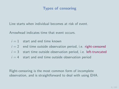
Line starts when individual becomes at risk of event.

Arrowhead indicates time that event occurs.

i = 1 start and end time known

i = 2 end time outside observation period, i.e. right-censored

i = 3 start time outside observation period, i.e. left-truncated

i = 4 start and end time outside observation period

Right-censoring is the most common form of incompleteobservation, and is straightforward to deal with using EHA.

8 / 183

Right-censoring

Right-censoring is the most common form of censoring.Durations are right-censored if the event has not occurred bythe end of the observation period.

- E.g. in a study of divorce, most respondents will still bemarried when last observed

Excluding right-censored observations (e.g. still married) leadsto bias and may drastically reduce sample size

Usually assume censoring is non-informative

9 / 183

Right-censoring: Non-informative assumption

We retain right-censored observations under the assumption thatcensoring is non-informative, i.e. event times are independent ofcensoring mechanism (like the ‘missing at random’ assumption).

Assume individuals are not selectively withdrawn from the samplebecause they are more or less likely to experience an event. May bequestionable in experimental research, e.g. if more susceptibleindividuals were selectively withdrawn (or dropped out) from a‘treatment’ group.

10 / 183

Event times and censoring times

Denote the event time (also known as duration, failure or survivaltime) by the random variable T .

ti event time for individual i

δi censoring/event indicator

= 1 if uncensored (i.e. observed to have event)

= 0 if censored

But for a right-censored case, we do not observe ti . We observeonly the time at which they were censored, ci .

Our outcome variable is yi = min(ti , ci ).

Our observed data are (yi , δi ).11 / 183

Descriptive Analysis

12 / 183

The hazard function

A key quantity in EHA is the hazard function:

h(t) = lim∆t→0

Pr(t ≤ T < t + ∆t|T ≥ t)

∆t

where the numerator is the probability that an event occurs duringa very small interval of time [t, t + ∆t), given that no eventoccurred before time t.

We divide by the width of the interval, ∆t, to get a rate.

h(t) is also known as the transition rate, the instantaneous risk, orthe failure rate.

13 / 183

The survivor function

Another useful quantity in EHA is the survivor function:

S(t) = Pr(T ≥ t)

the probability that an individual does not have the event before t,or ‘survives’ until at least t.

Its complement is the cumulative distribution function:

F (t) = 1− S(t) = Pr(T < t)

the probability that an individual has the event before t.

14 / 183

Non-parametric estimation of h(t)

Group time so that t is now an interval of time (duration mayalready by grouped, e.g. in months or years).

r(t) is number at ‘risk’ of experiencing event at start of interval td(t) is number of events (’deaths’) observed during tw(t) is number of censored cases (’withdrawals’) in interval t

The life table (or actuarial) estimator of h(t) is

h(t) =d(t)

r(t)− w(t)

Note. Assumes censoring times are spread uniformly across interval t.

Some estimators have r(t)− 0.5w(t) as the denominator, or ignore

censored cases.

15 / 183

Estimation of S(t)

The survivor function for interval t can be estimated from h(t) as:

S(t) = [1− h(1)]× [1− h(2)] . . .× [1− h(t − 1)]

= S(t − 1)× [1− h(t − 1)]

E.g. probability of surviving to the start of 3rd interval

= probability no event in 1st interval and no event in 2nd interval

= S(3) = [1− h(1)]× [1− h(2)]

16 / 183

Example: Time to 1st partnership

t r(t) d(t) w(t) h(t) S(t)

16 500 9 0 0.02 1

17 491 20 0 0.04 0.98

18 471 32 0 0.07 0.94

19 439 52 0 0.12 0.88

20 387 49 0 0.13 0.77

. . . . . .

. . . . . .

32 39 3 0 0.08 0.08

33 36 1 35 0.03 0.07

Source: National Child Development Study (1958 birth cohort). Note

that respondents were interviewed at age 33, so there is no censoring

before then.17 / 183

Example of interpretation

Event is partnering for the first time.

’Survival’ here is remaining single.

h(16) = 0.02 so 2% partnered before age 17

h(20) = 0.13 so, of those who were unpartnered at their 20thbirthday, 13% partnered before age 21

S(20) = 0.77 so 77% had not partnered by age 20

18 / 183

Hazard of 1st partnership

If an individual has not partnered by their late 20s, their chance ofpartnering declines thereafter.

19 / 183

Survivor function: Probability of remaining unpartnered

Note that the survivor function will always decrease with time.The hazard function may go up and down.

20 / 183

Continuous-time Models

21 / 183

Introducing covariates: Event history modelling

There are many different types of event history model, which varyaccording to:

Assumptions about the shape of the hazard function

Whether time is treated as continuous or discrete

Whether the effects of covariates can be assumed constantover time (proportional hazards)

22 / 183

The Cox proportional hazards model

The most commonly applied model is the Cox model which:

Makes no assumptions about the shape of the hazard function

Treats time as continuous

Assumes that the effects of covariates are constant over time(although this can be modified)

23 / 183

The Cox proportional hazards model

hi (t) is the hazard for individual i at time t

xi is a vector of covariates (for now assumed fixed over time) withcoefficients β

h0(t) is the baseline hazard, i.e. the hazard when xi = 0

The Cox model can be written:

hi (t) = h0(t) exp(βxi )

or sometimes as:

log hi (t) = log h0(t) + βxi

An individual’s hazard depends on t through h0(t) which is leftunspecified, so no need to make assumptions about the shape ofthe hazard.

24 / 183

Cox model: Interpretation (1)


Covariates have a multiplicative effect on the hazard.

For each 1-unit increase in x the hazard is multiplied by exp(β).

To see this, consider a binary x coded 0 and 1:

xi = 0 =⇒ hi (t) = h0(t)

xi = 1 =⇒ hi (t) = h0(t) exp(β)

So exp(β) is the ratio of the hazard for x = 1 to the hazard forx = 0, called the relative risk or hazard ratio.

25 / 183

Cox model: Interpretation (2)

exp(β) = 1 implies no effect of x on the hazard

exp(β) > 1 implies a positive effect on the hazard, i.e. highervalues of x are associated with shorter durations

- e.g. exp(β) = 2.5 implies an increase in h(t) by a factor of(2.5− 1)× 100 = 150% for a 1-unit increase in x

exp(β) < 1 implies a negative effect on the hazard, i.e. lowervalues of x are associated with longer durations

- e.g. exp(β) = 0.6 implies a decrease in h(t) by a factor of(1− 0.6)× 100 = 40% for a 1-unit increase in x

26 / 183

Example: Gender effects on age at 1st partnership

The log-hazard of forming the 1st partnership at age t is 0.4points higher for women than for men

The hazard of forming the 1st partnership at age t isexp(0.40) = 1.49 times higher for women than for men

Women partner at a younger age than men

27 / 183

The proportional hazards assumption

Consider a model with a single covariate x and two individualswith different values denoted by x1 and x2.

The proportional hazards model is written:


So the ratio of the hazards for individual 1 to individual 2 is:

h1(t)

h2(t)=

exp(βx1)

exp(βx2)

which does not depend on t. i.e. the effect of x is the same at alldurations t.

28 / 183

Example of (a) proportional and (b) non-proportional

hazards for binary x

29 / 183

Estimation of the Cox model

All statistical software packages have in-built procedures forestimating the Cox model. The input data are each individual’sduration yi and censoring indicator δi .

The data are restructured before estimation (although this ishidden from the user), and the Cox model is then estimated usingPoisson regression.

We will look at this data restructuring to better understand themodel and its relationship with the discrete-time approach. Butnote that you do not have to do this restructuring yourself!

30 / 183

Creation of risks sets

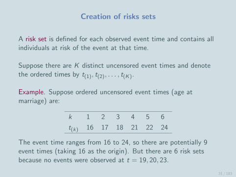
A risk set is defined for each observed event time and contains allindividuals at risk of the event at that time.

Suppose there are K distinct uncensored event times and denotethe ordered times by t(1), t(2), . . . , t(K).

Example. Suppose ordered uncensored event times (age atmarriage) are:

k 1 2 3 4 5 6

t(k) 16 17 18 21 22 24

The event time ranges from 16 to 24, so there are potentially 9event times (taking 16 as the origin). But there are 6 risk setsbecause no events were observed at t = 19, 20, 23.

31 / 183

Risk set based file

Consider records for 3 individuals:

individual i yi δi1 21 12 18 03 16 1

↓individual i risk set k t(k) yki (event

at t(k))1 1 16 01 2 17 01 3 18 01 4 21 12 1 16 02 2 17 02 3 18 03 1 16 1

32 / 183

Results from fitting Cox model

Hazard of partnering at age t is (1.48−1)×100 = 48% higherfor women than for men (i.e. W partner quicker than M)

Being in full-time education decreases the hazard by(1− 0.36)× 100 = 64%

33 / 183

Discrete-time Models

34 / 183

Discrete-time data

In social research, event history data are usually collected:

retrospectively in a cross-sectional survey, where dates arerecorded to the nearest month or year, OR

prospectively in waves of a panel study (e.g. annually)

Both give rise to discretely-measured durations.

Also called interval-censored because we only know that an eventoccurred at some point during an interval of time.

35 / 183

Data preparation for a discrete-time analysis

We must first restructure the data.

We expand the event times and censoring indicator (yi , δi ) to asequence of binary responses {yti} where yti indicates whether anevent has occurred in time interval [t, t + 1).

The required structure is very similar to the risk set-based file forthe Cox model, but the user has to do the restructuring ratherthan the software.

Also we now have a record for every time interval (not risk sets,i.e. intervals where events occur).

36 / 183

Data structure: The person-period file

individual i yi δi1 21 12 33 0

↓individual i t yti1 16 01 17 0. . .1 20 01 21 12 16 02 17 0. . .2 32 02 33 0

37 / 183

Discrete-time hazard function

Denote by pti the probability that individual i has an event duringinterval t, given that no event has occurred before the start of t.

pti = Pr(yti = 1|yt−1,i = 0)

pti is a discrete-time approximation to the continuous-time hazardfunction hi (t).

Call pti the discrete-time hazard function.

38 / 183

Discrete-time logit model

After expanding the data fit a binary response model to yti , e.g. alogit model:

log

(pti

1− pti

)= αDti + βxti

pti is the probability of an event during interval t

Dti is a vector of functions of the cumulative duration by interval twith coefficients α

xti is a vector of covariates (time-varying or constant over time)with coefficients β

39 / 183

Modelling the time-dependency of the hazard

Changes in pti with t are captured in the model by αDti , thebaseline hazard function.

Dti has to be specified by the user. Options include:

Polynomial of order p

αDti = α0 + α1t + . . .+ αptp

Step function

αDti = α1D1 + α2D2 + . . .+ αqDq

where D1, . . . ,Dq are dummies for time intervals t = 1, . . . , q andq is the maximum observed event time. If q large, categories maybe grouped to give a piecewise constant hazard model.

40 / 183

Discrete-time analysis of age at 1st partnership

Two covariates: FEMALE and FULLTIME (time-varying)

We consider two forms of αDti :

Step function: dummy variable for each year of age, 16-33

Quadratic function: include t and t2 as explanatory variables

41 / 183

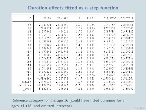
Duration effects fitted as a step function

Reference category for t is age 16 (could have fitted dummies for all

ages, t1-t18, and omitted intercept)42 / 183

Comparison of Cox and logit estimates for age at 1st

partnership

Cox Logit

Variable β se(β) β se(β)

Female 0.394 0.093 0.468 0.102

Fulltime(t) −1.031 0.190 −1.133 0.197

Same substantive conclusions, but:

Cox estimates are effects on log scale, and exp(β) are hazardsratios (relative risks)

Logit estimates are effects on log-odds scale, and exp(β) arehazard-odds ratios

43 / 183

When will Cox and logit estimates be similar?

In general, Cox and logit estimates will get closer as thehazard function becomes smaller because:

log(h(t)) ≈ log(

h(t)1−h(t)

)as h(t)→ 0.

The discrete-time hazard will get smaller as the width of thetime intervals become smaller.

A discrete-time model with a complementary log-log link,log(− log(1− pt)) , is an approximation to the Coxproportional hazards model, and the coefficients are directlycomparable.

44 / 183

Duration effects fitted as a quadratic

Approximating step function by a quadratic leads to little changein estimated covariate effects.

Estimates from step function model were 0.468 (SE = 0.102) forFemale and −1.133 (SE = 0.197) for Fulltime.

45 / 183

Non-proportional hazards

So far we have assumed that the effects of x are the same forall values of t

It is straightforward to relax this assumption in a discrete-timemodel by including interactions between x and t in the model

Test for non-proportionality by testing the null hypothesis thatthe coefficients of the interactions between x and t are allequal to zero, using likelihood ratio test

46 / 183

Allowing and testing for non-proportional effects of

gender on timing of 1st partnership

Add interactions: t fem = t × female and tsq fem = t2 × female

Likelihood-ratio statistic comparing main effects and interactionmodels = 2(1332.5− 1328.0) = 9 on 2 d.f., p-value = 0.011

Conclude that interaction effects are significantly different fromzero, i.e. effect of gender is non-proportional

47 / 183

Predicted log-odds of partnering: Proportional gender

effects

48 / 183

Predicted log-odds of partnering: Non-proportional

gender effects

49 / 183

2. Multilevel models for recurrentevents and unobserved heterogeneity

50 / 183

Unobserved Heterogeneity

51 / 183

What is unobserved heterogeneity?

Some individuals will be at higher risk of an event thanothers, and it is unlikely the reasons for this variability will befully captured by covariates

The presence of unmeasured individual-specific(time-invariant) risk factors leads to unobserved heterogeneityin the hazard

Unobserved heterogeneity is also referred to as frailty,especially in biostatistics (more ‘frail’ individuals have a highermortality risk)

52 / 183

Consequences of unobserved heterogeneity

If there are individual-specific unobserved factors that affect thehazard, the observed form of the hazard function at the aggregatepopulation level will tend to be different from the individual-levelhazards.

For example, even if the hazards of individuals in a population areconstant over time, the population hazard (averaged acrossindividuals) will be time-dependent, typically decreasing.

This may be explained by a selection effect operating onindividuals.

53 / 183

Selection effect of unobserved heterogeneity

If a population is heterogeneous in its susceptibility to experiencingan event, high risk individuals will tend to have the event first,leaving behind lower risk individuals.

Therefore as t increases the population is increasingly depleted ofthose individuals most likely to experience the event, leading to adecrease in the population hazard.

Because of this selection, we may see a decrease in the populationhazard even if individual hazards are constant (or even increasing).

54 / 183

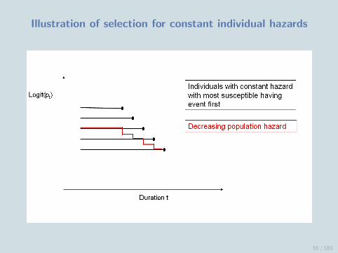
Illustration of selection for constant individual hazards

55 / 183

Impact of unobserved heterogeneity on

duration effects

If unobserved heterogeneity is incorrectly ignored:

A positive duration dependence will be understated (so anincreasing baseline hazard will increase more sharply afteraccounting for UH)

A negative duration dependence will be overstated

Note also that coefficients from random effects and traditionallogit models have a different interpretation (see later).

56 / 183

Allowing for unobserved heterogeneity in a

discrete-time model

We can introduce a random effect which representsindividual-specific unobservables:

log

(pti

1− pti

)= αDti + βxti + ui

pti is the probability of an event during interval t

Dti is a vector of functions of the cumulative duration by interval twith coefficients α

xti a vector of covariates with coefficients β

ui ∼ N(0, σ2u) allows for unobserved heterogeneity (‘frailty’)

between individuals due to time-invariant omitted variables57 / 183

Estimation of discrete-time model with unobserved

heterogeneity

We can view the person-period dataset as a 2-level structurewith time intervals (t) nested within individuals (i)

The discrete-time logit model with a random effect ui tocapture unobserved heterogeneity between individuals is anexample of a 2-level random intercept logit model

The model can be fitted using routines/software for multilevelbinary outcomes, e.g. Stata xtlogit

58 / 183

Results from analysis of 1st partnership

without (1) and with (2) unobserved heterogeneity

Model 1 Model 2

Est. (SE) Est. (SE)

t 0.367 (0.056) 0.494 (0.122)

t2 −0.018 (0.003) −0.020 (0.004)

Female 0.469 (0.102) 0.726 (0.215)

Fulltime −1.128 (0.186) −1.187 (0.208)

Cons −3.368 (0.237) −4.134 (0.646)

σu − − 0.920 (0.400)

Likelihood-ratio test statistic for test of H0 : σu = 0 is 3.74 on 1d.f., p=0.027 (one-sided test as σu must be non-negative).

59 / 183

More on comparing coefficients from random effects

and single-level logit models

In our analysis of age at 1st partnership, we saw that the positiveeffect of age (‘duration’) was understated if unobservedheterogeneity was ignored (as in Model 1).

Note also, however, that the effects of Female and Fulltime havealso changed. In both cases, the magnitude of the coefficients hasincreased after accounting for unobserved heterogeneity.

This can be explained by a scaling effect.

60 / 183

Scaling effect of introducing ui (1)

To see the scaling effect, consider the latent variable (threshold)representation of the discrete-time logit model.

Consider a latent continuous variable y∗ that underlies observedbinary y such that:

yti =

{1 if y∗ti ≥ 0

0 if y∗ti < 0

Threshold model

y∗ti = αDti + βxti + ui + e∗ti

e∗ti ∼ standard logistic (with variance ' 3.29) → logit model

e∗ti ∼ N(0, 1) → probit model

So the level 1 residual variance, var(e∗ti ), is fixed.

61 / 183

Scaling Effect of Introducing ui (2)

Single-level logit model expressed as a threshold model:

y∗ti = αDti + βxti + e∗ti

var(y∗ti |xti ) = var(e∗ti ) = 3.29

Now add random effects:

y∗ti = αDti + βxti + ui + e∗ti

var(y∗ti |xti ) = var(ui ) + var(e∗ti ) = σ2u + 3.29

Adding random effects has increased the residual variance→ scale of y∗ stretched out→ α and β increase in absolute value.

62 / 183

Scaling Effect of Introducing ui (3)

Denote by βRE the coefficient from a random effects model, andβSL the coefficient from the corresponding single-level model.

The approximate relationship between these coefficients (for a logitmodel) is:

βRE = βSL√σ2u + 3.29

3.29

Replace 3.29 by 1 to get expression for relationship between probitcoefficients.

Note that the same relationship would hold for duration effects α ifthere was no selection effect. In general, both selection and scalingeffects will operate on α.

63 / 183

Time to 1st partnership: Interpretation of coefficients

from the frailty model

For a given individual the odds of entering a partnership atage t when in FT education are exp(−1.19) = 0.30 times theodds when not in FT education.

- This interpretation is useful because Fulltime is time-varyingwithin an individual

For 2 individuals with the same random effect value the oddsare exp(0.73) = 2.08 times higher for a woman than for a man

- This interpretation is less useful, but we can ‘average out’random effect to obtain population-averaged predictedprobabilities

64 / 183

Population-averaged predicted probabilities

The probability of an event in interval t for individual i is:

pti =exp(αDti + βxti + ui )

1 + exp(αDti + βxti + ui )

where we substitute estimates of α, β, and ui to get predictedprobabilities.

Rather than calculating probabilities for each record ti , however,we often want predictions for specific values of x. We do this by’averaging out’ the individual unobservables ui .

65 / 183

Population-averaged predictions via simulation

Suppose we have 2 covariates, x1 and x2, and we want the meanpredicted pt for values of x1 holding x2 constant.

To get predictions for t = 1, . . . , q and x1 = 0, 1:

1. Set t = 1 and x1ti=0 for each record ti , retaining observedx2ti

2. Generate ui for each individual i from N(0, σ2u)

3. Compute predicted pt for each record ti based on x1ti = 0,observed x2ti , generated ui , and (α, β)

4. Take mean of predictions to get mean pt for t = 1 and x1 = 0

5. Repeat 1-4 for t = 2, . . . , q

6. Repeat 1-5 for x1ti = 1

66 / 183

Recurrent Events

67 / 183

Multilevel event history data

Multilevel event history data arise when events are repeatable (e.g.births, partnership dissolution) or individuals are organised ingroups.

Suppose events are repeatable, and define an episode as acontinuous period for which an individual is at risk of experiencingan event, e.g.

Event Episode duration

Birth Duration between birth k − 1 and birth k

Marital dissolution Duration of marriage

Denote by yij the duration of episode i of individual j , which isfully observed if an event occurs (δij = 1) and right-censored if not(δij = 0).

68 / 183

Data structure: the person-period-episode file

individual j episode i yij δij

1 1 2 1

1 2 3 0

↓individual j episode i t ytij

1 1 1 0

1 1 2 1

1 2 1 0

1 2 2 0

1 2 3 0

69 / 183

Problem with analysing recurrent events

We cannot assume that the durations of episodes from the sameindividual are independent.

There may be unobserved individual-specific factors (i.e. constantacross episodes) which affect the hazard of an event for allepisodes, e.g. ‘taste for stability’ may influence risk of leaving ajob.

The presence of such unobservables, and failure to account forthem in the model, will lead to correlation between durations ofepisodes from the same individual.

70 / 183

Multilevel discrete-time model for recurrent events

Multilevel (random effects) discrete-time logit model:

log

(ptij

1− ptij

)= αDtij + βxtij + uj

ptij is the probability of an event during interval t

Dtij is a vector of functions of the cumulative duration by intervalt with coefficients α

xtij a vector of covariates (time-varying or defined at the episode orindividual level) with coefficients β

uj ∼ N(0, σ2u) allows for unobserved heterogeneity (‘shared frailty’)

between individuals due to time-invariant omitted variables71 / 183

Multilevel model for recurrent events: Notes

The model for recurrent events is essentially the same as the(single-level) model for unobserved heterogeneity

- Both can be estimated using multilevel modellingsoftware/routines

Recurrent events allow better identification of the randomeffect variance σ2

u

Allow for non-proportional effects of covariate x by includinginteraction between x and functions of t in D

Can allow duration and covariate effects to vary acrossepisodes

- Include a dummy for order of event and interact with t and x

72 / 183

Example: Women’s employment transitions

Analyse duration of non-employment (unemployed or out oflabour market) episodes

- Event is entry (1st episode) or re-entry (2nd + episodes) intoemployment

Data are subsample from British Household Panel Study(BHPS): 1399 women and 2284 episodes

Durations grouped into years ⇒ 15,297 person-year records

Baseline hazard is step function with yearly dummies fordurations up to 9 years, then single dummy for 9+ years

Covariates include time-varying indicators of number and ageof children, age, marital status and characteristics of previousjob (if any)

73 / 183

Multilevel logit results for transition to employment:

Baseline hazard and unobserved heterogeneity

Variable Est. (se)

Duration non-employed (ref is < 1 year)

[1,2) years −0.646* (0.104)

[2,3) −0.934* (0.135)

[3,4) −1.233* (0.168)

[4,5) −1.099* (0.184)

[5,6) −0.944* (0.195)

[6,7) −1.011* (0.215)

[7,8) −1.238* (0.249)

[8,9) −1.339* (0.274)

≥ 9 years −1.785* (0.175)

σu (SD of woman random effect) 0.662* (0.090)

* p < 0.574 / 183

Multilevel logit results for transition to employment:

Presence and age of children

Variable Est. (se)

Imminent birth (within 1 year) −0.842* (0.125)

No. children age ≤ 5 yrs (ref=0)

1 child −0.212* (0.097)

≥ 2 −0.346* (0.143)

No. children age > 5 yrs (ref=0)

1 child 0.251 (0.118)

≥ 2 0.446* (0.117)

* p < 0.5

75 / 183

Multilevel logit analysis of employment:

Main conclusions

Unobserved heterogeneity. Significant variation betweenwomen. Deviance = 23.5 on 1 df; p<0.01

Duration effects. Probability of getting a job decreases withduration out of employment

Presence/age of children. Probability of entering employmentlower for women who will give birth in next year or with youngchildren, but higher for those with older children

Other covariates. Little effect of age, but increased chance ofentering employment for women who are cohabiting, havepreviously worked, whose last job was full-time, and whoseoccupation is ‘professional, managerial or technical’

76 / 183

Grouping time intervals

When we move to more complex models, a potential problem withthe discrete-time approach is that the person-period file can bevery large (depending on sample size and length of the observationperiod relative to the width of discrete-time intervals).

It may be possible to group time intervals, e.g. using 6-monthrather than monthly intervals.

BUT we must assume the hazard and values of covariates areconstant within grouped intervals.

77 / 183

Analysing grouped intervals

If we have grouped time intervals, we need to allow for differentlengths of exposure time within these intervals.

e.g. for any 6-month interval some individuals will have the eventor be censored after the 1st month while others will be exposed forthe full 6 months.

Denote by ntij the exposure time in grouped interval t of episode ifor individual j . (Note: Intervals do not need to be the samewidth.)

Fit binomial logit model for grouped binary data, with response ytijand denominator ntij (e.g. using the binomial() option in theStata xtmelogit command)

78 / 183

Example of grouped time intervals

Suppose an individual is observed to have an event during the 17thmonth of exposure, and we group durations into six-monthintervals (t). Instead of 17 monthly records we would have threesix-monthly records:

j i t ntij ytij

1 1 1 6 0

1 1 2 6 0

1 1 3 5 1

79 / 183

Software for Recurrent Events

Essentially multilevel models for binary responses

Mainstream software: e.g. Stata (xtlogit), SAS (PROCNLMIXED)

Specialist multilevel modelling software: e.g. MLwiN (also viarunmlwin in Stata), SABRE, aML

80 / 183

3. Modelling transitions betweenmultiple states

81 / 183

States in Event Histories

In the models considered so far, there is a single event (ortransition) of interest. We model the duration to this event fromthe point at which an individual becomes “at risk”. We can thinkof this as the duration spent in the same state.

E.g.

In the analysis of transitions into employment we model theduration in the non-employment state

In a study of marital dissolution we model the duration in themarriage state

More generally, we may wish to model transitions in the otherdirection (e.g. into non-employment or marriage formation) andpossibly other transitions.

82 / 183

Examples of Multiple States

Usually individuals will move in and out of different states overtime, and we wish to model these transitions.

Examples:

Employment states: employed full-time, employed part-time,unemployed, out of the labour market

Partnership states: marriage, cohabitation, single (not inco-residential union)

We will begin with models for transitions between two states, e.g.non-employment (NE) ↔ employment (E)

83 / 183

Transition Probabilities for Two States

Suppose there are two states indexed by s (s = 1, 2), and Stijindicates the state occupied by individual j during interval t ofepisode i .

Denote by ytij a binary variable indicating whether any transitionhas occurred during interval t, i.e. from state 1 to 2 or from state2 to 1.

The probability of a transition from state s during interval t, giventhat no transition has occurred before the start of t is:

pstij = Pr(ytij = 1|yt−1,ij = 0, Stij = s), s = 1, 2

Call pstij a transition probability or discrete-time hazard for state s.

84 / 183

Event History Model for Transitions between 2 States

Multilevel two-state logit model:

log

(pstij

1− pstij

)= αsDstij + βsxstij + usj ,

pstij is the probability of a transition from state s during interval t

Dstij is a vector of functions of cumulative duration in state s byinterval t with coefficients αs

xstij a vector of covariates affecting the transition from state s withcoefficients βs

usj allows for unobserved heterogeneity between individuals in theirprobability of moving from state s. Assume uj = (u1j , u2j) ∼bivariate normal.

85 / 183

Random Effect Covariance in a Two-State Model

We assume the state-specific random effects usj follow a bivariatenormal distribution to allow for correlation between theunmeasured time-invariant influences on each transition.

For example, a highly employable person may have a low chance ofleaving employment and a high chance of entering employment,leading to cov(u1j , u2j) < 0.

Allowing for cov(u1j , u2j) 6= 0 means that the equations for statess = 1, 2 must be estimated jointly. Estimating equations separatelyassumes that cov(u1j , u2j) = 0.

86 / 183

Data Structure for Two-State Model (1)

Start with an episode-based file.

E.g. employment (E) ↔ non-employment (NE) transitions

j i Stateij tij δij Ageij

1 1 E 3 1 16

1 2 NE 2 0 19

Note: (i) t in years; (ii) δij = 1 if a transition (event) occurs, 0 ifcensored; (iii) Age in years at start of episode

87 / 183

Data Structure for Two-State Model (2)

Convert episode-based file to discrete-time format with one recordper interval t:

t ytij Eij NEij EijAgeij NEijAgeij

1 0 1 0 16 0

2 0 1 0 16 0

3 1 1 0 16 0

1 0 0 1 0 19

2 0 0 1 0 19

Note: Eij a dummy for employment, NEij a dummy fornon-employment.

88 / 183

Example: Non-Employment ↔ Employment

corr(u1j , u2j)=0.59, se=0.13, so large positive residualcorrelation between E → NE and NE → E

- Women with high chance of entering E tend to have a highchance of leaving E

- Women with low chance of entering E tend to have a lowchance of leaving E

Positive correlation arises from two sub-groups: short spells ofE and NE, and longer spells of both types

89 / 183

Comparison of Selected Coefficients for NE → E

Only coefficients of covariates relating to employment historychange:

Single-state Multistate

Ever worked 2.936 2.677

Previous job part-time −0.441 −0.460

So positive effect of ‘ever worked’ has weakened, and negativeeffect of ‘part-time’ has strengthened.

90 / 183

Why Decrease in Effect of ‘Ever Worked’ on NE → E?

Direction of change from single-state to multistate (2.936 to2.677) is in line with positive corr(u1j , u2j) in multistate model.

Women in ‘ever worked’ must have made E → NE transition

Positive correlation between E → NE and NE → E leads todisproportionate presence of women with high NE → E rateamong ‘ever worked’

These women push up odds of NE → E among ‘ever worked’(inflating estimate) if residual correlation uncontrolled

91 / 183

Why Increase in Effect of Previous Part-Time Job on

NE → E?

Strengthening of negative effect when moving to the multistatemodel (−0.441 to −0.460) is also in line with positivecorr(u1j , u2j).

Women with tendency towards less stable employment (withhigh rate of E → NE) selected into part-time work

Positive correlation between E → NE and NE → E leads todisproportionate presence of women with high NE → E rate in‘previous PT’ category

These women push up odds of NE → E in ‘previous PT’(reducing ‘true’ negative effect of PT) if residual correlationuncontrolled

92 / 183

Autoregressive Models for Two States

An alternative way of modelling transitions between states is toinclude the lagged response as a predictor rather than the durationin the current state.

The response ytij now indicates the state occupied at the start ofinterval t rather than whether a transition has occurred, i.e.

ytij =

{1 if in state 1

0 if in state 2

93 / 183

1st Order Autoregressive Model

An AR(1) model for the probability that individual j is in state 1 att, ptj is:

log

(ptj

1− ptj

)= α + βxtj + γyt−1,j + uj

α is an intercept term

γ is the effect of the state occupied at t − 1 on the log-odds ofbeing in state 1 at t

uj ∼ N(0, σ2u) is an individual-specific random effect

94 / 183

Interpretation of AR(1) Model

Suppose states are employment and unemployment. Common tofind those who have been unemployed in the past are more likely tobe unemployed in the future. Three potential explanations:

A causal effect of unemployment at t − 1 on beingunemployed at t (state dependence γ)

Unobserved heterogeneity, i.e. unmeasured individualcharacteristics affecting unemployment probability at all t(stable traits uj)

Non-stationarity, e.g. seasonality (not in current model)

The AR(1) model is commonly referred to as a state dependencemodel.

95 / 183

Transition Probabilities from the AR(1) Model

We model ptj = Pr(state 1 at start of interval t) = Pr(ytj = 1)

Suppose we fix xtj = 0 and uj = 0.

Probability of moving from state 1 to 2

Pr(ytj = 0|yt−1,j = 1) = 1− Pr(ytj = 1|yt−1,j = 1)

= 1− exp(α+γ)1+exp(α+γ)

Probability of moving from state 2 to 1

Pr(ytj = 1|yt−1,j = 0) =exp(α)

1 + exp(α)

96 / 183

Initial Conditions (1)

y may not be measured at the start of the process, e.g. we maynot have entire employment histories.

Can view as a missing data problem. Suppose we observe y at thestart of T intervals:

Observed (y1, . . . , yT )

Actual (y−k , . . . , y0,y1, . . . , yT )

where first k + 1 measures are missing.

We need to specify a model for y1 (not just condition on y1).

97 / 183

Initial Conditions (2)

In a random effects framework, we can specify a model for y1j andestimate jointly with the model for (y2j , . . . , yTj), e.g.

logit(p1j) = α1 + β1xt1j + λuj

logit(ptj) = α + β1xtj + γyt−1,j + uj , t > 1

Variants on the above are to set λ = 1 or to include differentrandom effect in equation for t = 1, e.g. u1j , and allow forcorrelation with uj in equation for t > 1.

The inclusion of λ allows the between-individual residual varianceto differ for t = 1 and t > 1.

98 / 183

Key Features of the AR(1) Model

All relevant information about the process up to t is capturedby yt−1 (1st order Markov assumption). This is why durationeffects are not included.

Because of the 1st order Markov assumption, there is noconcept of an ‘episode’ (which is why we drop the i subscript)

Effects of x (and time-invariant characteristics uj) are thesame for transitions from state 1 to 2, and from state 2 to 1

- But it is straightforward to allow for transition-specific effectsby interacting x with yt−1

99 / 183

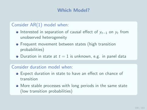
Which Model?

Consider AR(1) model when:

Interested in separation of causal effect of yt−1 on yt fromunobserved heterogeneity

Frequent movement between states (high transitionprobabilities)

Duration in state at t = 1 is unknown, e.g. in panel data

Consider duration model when:

Expect duration in state to have an effect on chance oftransition

More stable processes with long periods in the same state(low transition probabilities)

100 / 183

Software for Multiple States

Two-state duration model can be framed as a multilevelrandom coefficients model

- Coefficients for the two state dummies are intercepts whichvary randomly across individuals to give random effects foreach state

- Software options as for one-state recurrent events model, butusing xtmelogit in Stata

Autoregressive model (with equation for t = 1) can also befitted as a random coefficient model, but more general models(e.g. allowing different residual variances for t = 1 and t > 1)require specialist software such as Sabre and aML

101 / 183

4. Competing risks

102 / 183

More than Two states

In general there may be multiple states, possibly with differentdestinations from each state. E.g. consider transitions betweenmarriage (M), cohabitation (C) and single (S).

103 / 183

Competing risks

We will begin with the special case where we are interested intransitions from one origin state, but there is more than onedestination or type of transition.

Assume these destinations are mutually exclusive. We call these‘competing risks’.

Origin state Competing risks

Alive Different causes of death

Employed Sacked, redundancy, switch job, leave labour market

Single Marriage, cohabitation

104 / 183

Approaches to Modelling Competing Risks

Suppose there are R types of transition/event. For each interval t(of episode i of individual j) we can define a categorical responseytij :

ytij =

{0 if no event in t

r if event of type r in t (r = 1, . . . ,R)

Analysis approaches

1. Multinomial model for ytij

2. Define binary response y(r)tij for event type r , treating all other

types of event as censored. Analyse using multivariateresponse model

105 / 183

Multinomial Logit Model

Define p(r)tij = Pr(ytij = r |yt−1,ij = 0) for r = 1, . . . ,R.

Estimate R equations contrasting event type r with ‘no event’:

log

p

(r)tij

p(0)tij

= α(r)D

(r)tij + β(r)x

(r)tij + u

(r)j , r = 1, . . . ,R

where (u(1)j , u

(2)j , . . . , u

(R)j ) ∼ multivariate normal.

Correlated random effects allows for shared unobserved risk factors.

106 / 183

Multivariate Binary Response Model

In the second approach to modelling competing risks we define, foreach interval t, R binary responses coded as:

y(r)tij =

{1 if event of type r in t

0 if event of any type other than r or no event in t

and estimate equations for each event type:

log

p

(r)tij

1− p(r)tij

= α(r)D

(r)tij + β(r)x

(r)tij + u

(r)j , r = 1, . . . ,R

where (u(1)j , u

(2)j , . . . , u

(R)j ) ∼ multivariate normal.

107 / 183

Logic Behind Treating Other Events as Censored

Suppose we are interested in modelling partnership formation,where an episode in the ‘single’ state can end in marriage orcohabitation.

For each single episode we can think of durations to marriage andcohabitation, t(M) and t(C).

We cannot observe both of these. If a single episode ends inmarriage, we observe only t(M) and the duration to cohabitation iscensored at t(M). A person who marries is removed from the riskof cohabiting (unless they become single again).

For uncensored episodes we observe min(t(M), t(C)).

108 / 183

Comparing Methods

Coefficients and random effect variances and covariances will bedifferent for the two models because the reference category isdifferent:

‘No event’ in the multinomial model

- Coefficients are effects on the log-odds of an event of type rrelative to ‘no event’

‘No event + any event other than r ’ in the multivariate binarymodel

- Coefficients are effects on the log-odds of an event of type rrelative to ‘no event of type r ’

However, predicted transition probabilities will in general be similarfor the two models.

109 / 183

Transition Probabilities

Multinomial model

p(r)tij =

exp(α(r)D(r)tij + β(r)x

(r)tij + u

(r)j )

1 +∑R

k=1 exp(α(k)D(k)tij + β(k)x

(k)tij + u

(k)j )

Multivariate binary model

p(r)tij =

exp(α(r)D(r)tij + β(r)x

(r)tij + u

(r)j )

1 + exp(α(r)D(r)tij + β(r)x

(r)tij + u

(r)j )

In each case, the ‘no event’ probability is p(0) = 1−∑Rk=1 p

(k).

To calculate probabilities for specific values of x, substituteu(r) = 0 or generate u(r) from multivariate normal distribution.

110 / 183

Example: Transitions to Full-time and Part-time Work

Selected results from bivariate model for binary responses, y (FT )

and y (PT )

NE → FT NE → PT

Variable Est (se) Est (se)

Imminent birth −1.19* (0.18) −0.26 (0.15)

1 kid ≤ 5 −1.27* (0.15) 0.60* (0.12)

2+ kids ≤ 5 −1.94* (0.27) 0.81* (0.17)

1 kid > 5 −0.42* (0.19) 0.80* (0.14)

2+ kids > 5 −0.26 (0.18) 1.24* (0.15)

So having kids (especially young ones) reduces chance of returningto FT work, but increases chance of returning to PT work.

111 / 183

Example: Random Effect Covariance Matrix

NE → FT NE → PT

NE → FT 1.49 (0.13)

NE → PT −0.05 (0.11) 0.98 (0.11)

Note: Parameters on diagonal are standard deviations, and the off-diagonal

parameter is the correlation. Standard errors in parentheses.

Correlation is not significant (deviance test statistic is < 1 on 1d.f.).

112 / 183

Dependency between Competing Risks

A well-known problem with the multinomial logit model is the‘independence of irrelevant alternatives’ (IIA) assumption

In the context of competing risks, IIA implies that theprobability of one event relative to ‘no event’ is independentof the probabilities of each of the other events relative to ‘noevent’

This may be unreasonable if some types of event can beregarded as similar

Note that the multivariate binary model makes the sameassumption

113 / 183

Dependency between Competing Risks: Example

Suppose we wish to study partnership formation: transitions fromsingle (S) to marriage (M) or to cohabitation (C).

Under IIA, assume probability of C vs. S is uncorrelated withprobability of M vs. S

E.g. if there is something unobserved (not in x) that made Minfeasible, we assume those who would have married distributethemselves between C and S in the same proportions as thosewho originally chose not to marry

But as M and C are similar, we might expect those who areprecluded from marriage to be more likely to cohabit ratherthan remain single (Hill, Axinn and Thornton, 1993,Sociological Methodology)

114 / 183

Relaxing the Independence Assumption

Including individual-specific random effects allows fordependence due to time-invariant individual characteristics(e.g. attitudes towards marriage/cohabitation)

But it does not allow for unmeasured factors that vary acrossepisodes (e.g. marriage is not an option if respondent or theirpartner is already married)

115 / 183

Modelling Transitions between More than 2 States

So far we have considered (i) transitions between two states, and(ii) transitions from a single state with multiple destinations.

We can bring these together in a general model, allowing fordifferent destinations from each state.

Example: partnership transitions

Formation: S → M, S → C

Conversion of C to M (same partner)

Dissolution: M → S, C → S (or straight to new partnership)

Estimate 5 equations simultaneously (with correlated randomeffects)

116 / 183

Example of Multiple States with Competing Risks

Contraceptive use dynamics in Indonesia. Define episode ofuse as continuous period of using same method ofcontraception

- 2 states: use and nonuse- Episode of use can end in 2 ways: discontinuation (transition

to nonuse), or method switch (transition within ‘use’ state)

Estimate 3 equations jointly: binary logit for nonuse → use,and multinomial logit for transitions from use

Details in Steele et al. (2004) Statistical Modelling

117 / 183

Selected Results: Coefficients and SEs

Use → nonuse Use → new method Nonuse → use

(Discontinuation) (Method switch)

Urban 0.13 (0.04) 0.06 (0.05) 0.26 (0.04)

SES

Medium −0.12 (0.05) 0.35 (0.07) 0.24 (0.05)

High −0.20 (0.05) 0.29 (0.08) 0.45 (0.05)

118 / 183

Random Effect Correlations from Alternative Models

Discontinuation Method switch Nonuse → use

Discontinuation 1

Method switch 0.020 1

0.011

Nonuse → use −0.783* 0.165* 1

−0.052 0.095

Model 1: Duration effects onlyModel 2: Duration + covariate effects

*Correlation significantly different from zero at 5% level

119 / 183

Random Effect Correlations: Interpretation

In ‘duration effects only’ model, there is a large negativecorrelation between random effects for nonuse → use and use→ nonuse

- Long durations of use associated with short durations ofnonuse

This is due to short episodes of postnatal nonuse followed bylong episodes of use (to space or limit future births)

- Correlation is effectively zero when we control for whetherepisode of nonuse follows a live birth (one of the covariates)

120 / 183

Software for Competing Risks

Multivariate binary response model can be framed as amultilevel random coefficients model

- Coefficients for the response dummies are intercepts whichvary randomly across individuals to give random effects foreach type of event

- Software options as for one-state recurrent events model, butusing xtmelogit in Stata

Multinomial model cannot currently be fitted in Stata (apartfrom via runmlwin). Other options include SAS (PROCNLMIXED), MLwiN and aML

121 / 183

5. Multiprocess models

122 / 183

Endogeneity in a 2-Level Continuous Response Model

Consider a 2-level random effects model for a continuous response:

yij = βxij + uj + eij

where xij is a set of covariates with coefficients β, uj is the level 2random effect (residual) ∼ N(0, σ2

u) and eij is the level 1 residual∼ N(0, σ2

e ).

One assumption of the model is that xij is uncorrelated with bothuj and eij , i.e. we assume that xij is exogenous.

This may be too strong an assumption. If unmeasured variablesaffecting yij also affect one or more covariates, then thosecovariates will be endogenous.

123 / 183

2-Level Endogeneity: Example

Suppose yij is birth weight of child i of woman j , and zij is thenumber of antenatal visits during pregnancy (an element of xij).

Some of the factors that influence birth weight may also influenceuptake of antenatal care; these may be characteristics of theparticular pregnancy (e.g. woman’s health during pregnancy) or ofthe woman (health-related attitudes/behaviour). Some of thesemay be unobserved.

i.e. y and z are to some extent jointly determined, and z isendogenous.

This will lead to correlation between z and u and/or e and, ifignored, a biased estimate of the coefficient of z and possiblycovariates correlated with z .

124 / 183

Illustration of Impact of Endogeneity at Level 1

Suppose the ‘true’ effect of zij on yij is positive, i.e. moreantenatal visits is associated with a higher birth weight.

Suppose that wij is ‘difficulty of pregnancy’. We would expectcorr(w , y) < 0, and corr(w , z) > 0.

If w is unmeasured it is absorbed into e, leading to corr(z , e) < 0.

If we ignore corr(z , e) < 0, the estimated effect of z on y will bebiased downwards.

The disproportionate presence of high w women among thosegetting more antenatal care (high z) suppresses the positive effectof z on y .

125 / 183

Illustration of Impact of Endogeneity at Level 2

As before, suppose the ‘true’ effect of z on y is positive, i.e. moreantenatal visits is associated with a higher birth weight.

Suppose that wj is ‘healthcare knowledge’ which is constant acrossthe observation period. We would expect corr(w , y) > 0, andcorr(w , z) > 0.

If w is unmeasured it is absorbed into u, leading to corr(z , u) > 0.

Question: What effect would ignoring corr(z , u) > 0 have on theestimated effect of z on y?

126 / 183

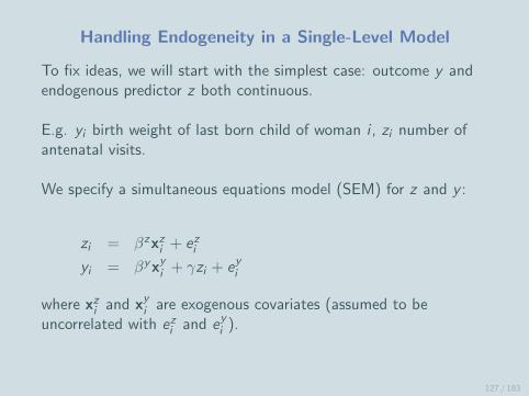
Handling Endogeneity in a Single-Level Model

To fix ideas, we will start with the simplest case: outcome y andendogenous predictor z both continuous.

E.g. yi birth weight of last born child of woman i , zi number ofantenatal visits.

We specify a simultaneous equations model (SEM) for z and y :

zi = βzxzi + eziyi = βyxyi + γzi + eyi

where xzi and xyi are exogenous covariates (assumed to beuncorrelated with ezi and eyi ).

127 / 183

Estimation

If corr(ezi , eyi ) = 0, OLS of the equation for yi is optimal.

Endogeneity of zi will lead to corr(ezi , eyi ) 6= 0 and an alternative

estimation procedure is required. The most widely used approachesare:

2-stage least squares (2SLS)

Joint estimation of equations for z and y (Full InformationMaximum Likelihood, FIML)

128 / 183

Estimation: 2-Stage Least Squares

1. OLS estimation of equation for zi and compute zi = βzxzi

2. OLS estimation of equation for yi replacing zi by prediction zi

3. Adjust standard errors in (2) to allow for uncertainty inestimation of zi

Idea: zi is ‘purged’ of the correlated unobservables ezi , so ziuncorrelated with eyi .

129 / 183

Estimation: FIML

Treat zi and yi as a bivariate response and estimate equationsjointly.

Usually assume ezi and eyi follow a bivariate normal distributionwith correlation ρzye .

Can be estimated in a number of software packages (e.g.mvreg in Stata or Sabre)

Sign of ρzye signals direction of bias

Generalises to mixed response types (e.g. binary z andduration y)

Generalises to clustered data (multilevel multivariate model)

130 / 183

Testing for Exogeneity of z

To test the null hypothesis that z is exogenous:

2SLS

Estimate yi = βyxyi + γzi + δezi + eyi via OLS

where ezi is the estimated residual from fitting the 1st stageequation for zi

Test H0 : δ = 0 using t (or Z) test.

FIML

Jointly estimate equations for zi and yi to get estimate of residualcorrelation ρzye .

Test H0 : ρzye = 0 using likelihood ratio test.

131 / 183

Identification

Whatever estimation approach is used, identification of thesimultaneous equations model for z and y requires covariateexclusion restrictions.

xzi should contain at least one variable that is not in xyi .

In our birth weight example, need to find variable(s) that predictantenatal visits (z) but not birth weight (y).

Call such variables instruments.

Note: The term ‘IV estimation’ is commonly used interchangeablywith 2SLS, but both methods require instruments.

132 / 183

Requirements of an Instrument (1)

Need to be able to justify, on theoretical grounds, that theinstrument affects z but not y (after controlling for z and othercovariates).

E.g. indicator of access to antenatal care may be suitableinstrument for no. visits, but only if services are allocatedrandomly (rare). Instruments can be very difficult to find.

If there is > 1 instrument, the model is said to be over-identified.

133 / 183

Requirements of an Instrument (1)

Testing over-identifying restrictions

Instruments should not affect y after controlling for z .

Fit the SEM with all but one instrument in the equation for y andcarry out a joint significance test of the included instruments. If therestrictions are valid, they should not have significant effects on y .

Instruments should be correlated with z

Carry out joint significance test of effects of instruments on z .

Also check how well instruments (together with other covariates)predict z . Bollen et al. (1995) suggest a simple probit for y ispreferred if R2 < 0.1.

134 / 183

Effect of Fertility Desires on Contraceptive Use (1)

Reference: Bollen, Guilkey and Mroz (1995), Demography.

Interested in the impact of number of additional children desired(z , continuous) on use of contraception (y , binary).

Unmeasured variable affecting both z and y could be ‘perceivedfecundity’.

Women who believe they have low chance of having a(nother)child may lower fertility desires and not use contraception →corr(ezi , e

yi ) > 0.

135 / 183


Expect ‘true’ effect of fertility desires (z) on contraceptive use (y)to be negative.

If residual correlation ignored, negative effect of z on y will beunderstated (may even estimate a positive effect)

Estimated effects of covariates correlated with z also biased(e.g. whether heard family planning message)

136 / 183


Cross-sectional data: z and y refer to time of survey.

Use 2SLS: OLS for z equation, probit for y .

Instruments: Indicators of health care facilities in community whenwoman was age 20 (supplementary data).

Results:

Residual correlation estimated as 0.07

Stronger negative effect of z after allowing for endogeneity(changes from −0.17 to −0.28), but large increase in SE

But fail to reject null that z is exogenous, so simple probit forcontraceptive use is preferred

137 / 183

Handling Endogeneity in a Multilevel Model

Let’s return to the multilevel case with yij the birth weight of childi of woman j , zij number of antenatal visits.

We specify a multilevel simultaneous equations (multiprocess)model for z and y :

zij = βzxzij + uzj + ezijyij = βyxyij + γzij + uyj + eyij

where uzj and uyj are normally distributed woman-level random

effects, and xzij and xyij are exogenous covariates (assumed to be

uncorrelated with uzj , uyj , ezij and eyij ).

138 / 183

Estimation

If corr(uzj , uyj ) = 0 and corr(ezij , e

yij ) = 0, the equation for yij can be

estimated as a standard multilevel model.

However, endogeneity of zij will lead to corr(uzj , uyj ) 6= 0 or

corr(ezij , eyij ) 6= 0 (or both).

If zij is endogenous we need to estimate equations for z and yjointly.

In the most general model, we assume (uzj , uyj ) ∼ bivariate normal

and (ezij , eyij ) ∼ bivariate normal. The SEM is a multilevel bivariate

response model.

139 / 183

Identification (1)

Identification of the full multilevel SEM for z and y , withcorr(uzj , u

yj ) 6= 0 and corr(ezij , e

yij ) 6= 0, requires covariate exclusion

restrictions:

xzij should contain at least one variable (an instrument) that is not

in xyij .

e.g. need to find variable(s) that predict antenatal visits (z) butnot birth weight (y).

Call such variables instruments.

BUT if one of the residual covariances is assumed equal to zero,covariate exclusions are not strictly necessary for identification.

140 / 183

Identification (2)

Suppose we are prepared to assume that endogeneity of z is due toa residual correlation at the woman level but not at the pregnancylevel, i.e.

corr(uzj , uyj ) 6= 0 but corr(ezij , e

yij ) = 0.

We are then assuming that bias in the estimated effect of numberof antenatal visits on birth weight is due to selection onunmeasured maternal characteristics that are fixed acrosspregnancies.

141 / 183

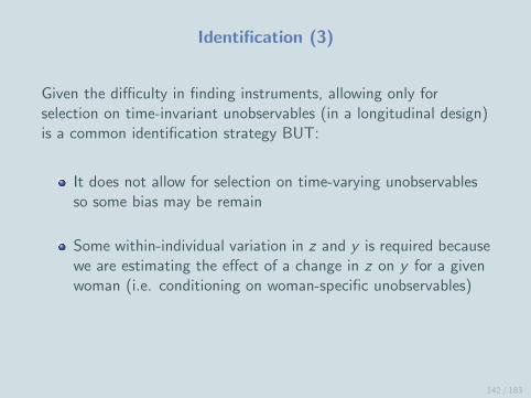
Identification (3)

Given the difficulty in finding instruments, allowing only forselection on time-invariant unobservables (in a longitudinal design)is a common identification strategy BUT:

It does not allow for selection on time-varying unobservablesso some bias may be remain

Some within-individual variation in z and y is required becausewe are estimating the effect of a change in z on y for a givenwoman (i.e. conditioning on woman-specific unobservables)

142 / 183

Allowing for Endogeneity in an Event History Model

Suppose that yij is the duration of episode i of individual j and zijis an endogenous variable. We first consider case where z iscontinuous and measured at the episode level.

We can extend our earlier recurrent events model to a SEM:

zij = βzxzij + uzj + ezij

log(

ptij1−ptij

)= αyDy

tij + βyxytij + γzij + uyj

where ptij is the probability of an event during interval t, αyDytij is

the baseline hazard, and xytij a vector of exogenous covariates.

We assume (uzj , uyj ) ∼ bivariate normal, i.e. we allow for selection

on time-invariant individual characteristics.

143 / 183

Examples of Multilevel SEM for Event History Data

More generally z can be categorical and can be defined at any level(e.g. time-varying or a time-invariant individual characteristic).

We will consider two published examples before returning to ouranalysis of women’s employment transitions:

The effect of premarital cohabitation (z) on subsequentmarital dissolution (y)

- Lillard, Brien & Waite (1995), Demography

The effect of access to family planning (z) on fertility (y)

- Angeles, Guilkey & Mroz (1998), Journal of the AmericanStatistical Association

144 / 183

Example 1: Premarital Cohabitation and Divorce

Couples who live together before marriage appear to have anincreased risk of divorce.

Is this a ‘causal’ effect of premarital cohabitation or due toself-selection of more divorce-prone individuals into premaritalcohabitation?

The analysis uses longitudinal data so observe women in multiplemarriages (episodes). For each marriage define 2 equations:

A probit model for premarital cohabitation (z)

A (continuous-time) event history model for maritaldissolution (y)

Each equation has a woman-specific random effect, uzj and uyj ,which are allowed to be correlated

145 / 183

Premarital Cohabitation and Divorce: Identification

Lillard et al. argue that exclusion restrictions are unnecessarybecause of ‘within-person replication’.

Nevertheless they include some variables in the cohabitationequation that are not in the dissolution equation:

Education level of woman’s parents

Rental prices and median home value in state

Sex ratio (indicator of ‘marriageable men/women’)

They examine the robustness of their conclusions to omitting thesevariables from the model.

146 / 183

Premarital Cohabitation and Divorce: Results (1)

Correlation between woman-specific random effects forcohabitation and dissolution estimated as 0.36.

Test statistic from a likelihood ratio test of the null hypothesis thatcorr(uzj , u

yj ) = 0 is 4.6 on 1 d.f. which is significant at the 5% level.

“There are unobserved differences across individuals which makethose who are most likely to cohabit before any marriage also mostlikely to end any marriage they enter.”

147 / 183

Premarital Cohabitation and Divorce: Results (2)

What is the impact of ignoring this residual correlation, andassuming premarital cohabitation is exogenous?

Estimated effect of cohabitation on log-hazard of dissolution

0.37 and strongly significant if corr(uzj , uyj ) = 0 assumed

-0.01 and non-significant if corr(uzj , uyj ) allowed to be non-zero

Conclude that, after allowing for selection, there is no associationbetween premarital cohabitation and marital dissolution.

148 / 183

Example 2: Access to Family Planning and Fertility

Does availability of family planning (FP) services lead to areduction in fertility in Tanzania?

Problem: FP clinics are unlikely to be placed at random. They arelikely to be targeted towards areas of greatest need, the type ofarea with high fertility.

Question: If true impact of access to FP is to increase birthspacing, how will ignoring targeted placement affect estimates ofthe impact?

149 / 183

Data and Measures

Birth histories collected retrospectively in 1992. Women nestedwithin communities, so have a 3-level structure: births (level 1),women (level 2), communities (level 3).

Constructed woman-year file for period 1970-1991 with ytij=1 ifwoman i in community j gave birth in year t. (Could have extrasubscript for birth interval as we model duration since last birth.)

Community survey on services conducted in 1994. Constructindicators of distance to hospital, health centre etc. in year t, ztj .Time-varying indicators derived from information on timing offacility placement.

150 / 183

Multiprocess Model for Programme Placement and

Fertility

The model consists of 4 equations:

Discrete-time event history model for probability of a birth inyear t with woman and community random effects

Logit models for placement of 3 types of FP facility incommunity j in year t with community random effects

Allow for correlation between community random effects forfertility and FP clinic placement.

Rather than assume normality, the random effects distribution isapproximated by a step function using a ‘discrete factor’ method.

151 / 183

Programme Placement and Fertility: Identification

The following time-varying variables are included in the FPplacement equations but not the fertility equation:

National government expenditure on health

Regional government expenditure on health

District population as fraction of national population

These are based on time series data at the national, regional andcommunity levels.

152 / 183

Programme Placement and Fertility: Findings

From simple analysis (ignoring endogeneity of programmeplacement) find hospitals have more impact on reducingfertility than health centres

But this analysis overstates impact of hospitals andunderstates effects of health centres

Controlling for endogenous programme placement reveals thathealth centres have more impact than hospitals

After controlling for endogenity, impact of FP facilities was45% larger than in simpler analysis

153 / 183

Modelling Correlated Event Processes

Now suppose that ztij is a time-varying endogenous predictor.

ztij is often the outcome of a related event process.

Example: Marital dissolution and fertility

yij is duration of marriage i of woman j

ztij is number of children from marriage i of woman j at time t,the outcome of the birth history by t

See Lillard (1993) and Lillard & Waite (1993).

154 / 183

Multiprocess Model SEM for 2 Interdependent Events

Simultaneous discrete-time event history equations:

logit(pztij) = αzDztij + βzxztij + uzj

logit(pytij) = αyDytij + βyxytij + γzij + uyj

We assume (uzj , uyj ) ∼ bivariate normal, i.e. we allow for selection

on time-invariant individual characteristics.

The model can be extended to include outcomes of the y processin the model for z .

155 / 183

Example: Marital Dissolution and Fertility

Lillard’s model has 2 (continuous-time) event history equations for:

hazard of conception (leading to a live birth) at time t ofmarriage i of woman j

hazard that marriage i of woman j ends at time t

Consider dummies for ztij , the number of children from marriage i ,in dissolution equation.

156 / 183

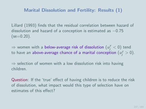
Marital Dissolution and Fertility: Results (1)

Lillard (1993) finds that the residual correlation between hazard ofdissolution and hazard of a conception is estimated as −0.75(se=0.20).

⇒ women with a below-average risk of dissolution (uyj < 0) tendto have an above-average chance of a marital conception (uzj > 0).

⇒ selection of women with a low dissolution risk into havingchildren.

Question: If the ‘true’ effect of having children is to reduce the riskof dissolution, what impact would this type of selection have onestimates of this effect?

157 / 183

Marital Dissolution and Fertility: Results (2)

Estimated effects (SE) of number of children from currentmarriage on log-hazard of dissolution before and after accountingfor residual correlation:

# children Before After

0 (ref) 0 0

1 −0.56 (0.10) −0.33 (0.11)

2+ −0.01 (0.05) 0.27 (0.07)

Selection of low dissolution risk women into categories 1 and 2+

158 / 183

Other Examples of Correlated Event Histories

Employment transitions and fertility (next example)

Partnership formation and employment

Residential mobility and fertility

Residential mobility and employment

Residential mobility and partnership formation/dissolution

159 / 183

Multiprocess Model for Entry into Employment and

Fertility (1)

At the start of the course (and in computer exercises) we fittedmultilevel models for the transition from non-employment (NE) toemployment (E) among British women.

Among the covariates was a set of time-varying fertility indicators:

Due to give birth within next year

Number of children aged ≤ 5 years

Number of children aged > 5 years

These are outcomes of the fertility process which might be jointlydetermined with employment transitions.

160 / 183

Multiprocess Model for Entry into Employment and

Fertility (2)

Denote by yNEtij and yBtij binary indicators for leavingnon-employment and giving birth during year t.

Estimate 2 simultaneous equations (both with woman-specificrandom effects):

Discrete-time logit for probability of a birth

Discrete-time logit for probability of NE → E (with fertiltyoutcomes as predictors)

Note: While we could model births that occur duringnon-employment, it would be more natural to model the wholebirth process (in both NE and E). In the following analysis, weconsider all births.

161 / 183

Estimation of Multiprocess Model

We can view the discrete-time multiprocess model as a multilevelbivariate response model for the binary responses yNEtij and yBtij .

Stack the employment and birth responses into a singleresponse column and define an index r which indicates theresponse type (e.g. r = 1 for NE and r = 2 for B)

Define dummies for r which we call r1 and r2 say

Multiply r1 and r2 by the covariates to be included in the NEand B equations respectively

Fit woman-level random effects to r1 and r2 and allow to becorrelated

162 / 183

Entry into Employment and Fertility: Residual

Correlation

Likelihood ratio test statistic for test of null hypothesis thatcorr(uNEj , uBj ) = 0 is 8 on 1 d.f.

⇒ reject the null and choose the multiprocess model.

Correlation between woman-level random effects, uNEj and uBj ,estimated as 0.34 (se=0.11).

The positive correlation implies that women whose unobservedcharacteristics are associated with a high probability of a birth(e.g. latent preference for childbearing) tend also to enteremployment quickly after a spell of non-employment.

163 / 183

Effects of Fertility Outcomes on Entry into Employment

Single process Multiprocess

Variable Est. (se) Est. (se)

Imminent birth (within 1 year) −0.84* (0.13) −1.01* (0.14)

No. children ≤ 5 yrs (ref=0)

1 child −0.21* (0.10) −0.35* (0.11)

≥ 2 −0.35* (0.14) −0.60* (0.17)

No. children > 5 yrs (ref=0)

1 child 0.25* (0.12) 0.18 (0.12)

≥ 2 0.45* (0.12) 0.27* (0.13)

* p < 0.5

Selection of women with high NE → E probability into categories 1 and ≥ 2

164 / 183

Multiple States and Correlated Processes

We can extend the multiprocess model to include transitionsbetween multiple states and further correlated processes.

E.g. we could model two-way transitions between NE and E jointlywith births, leading to 3 simultaneous equations and 3 correlatedrandom effects.

Stack employment transition and birth responses into a singlecolumn with a 3-category response indicator r (e.g. r=1 foremployment episodes, r=2 for non-employment episodes, r=3 forbirth intervals).

Create dummies for r and interact with covariates as for two-stateand multiprocess models.

165 / 183

Employment Transitions and Fertility: Random Effects

Correlation Matrix

NE → E E → NE Birth

NE → E 1

E → NE 0.62 (0.12) 1

Birth 0.45 (0.11) 0.23 (0.08) 1

Standard errors in brackets

166 / 183

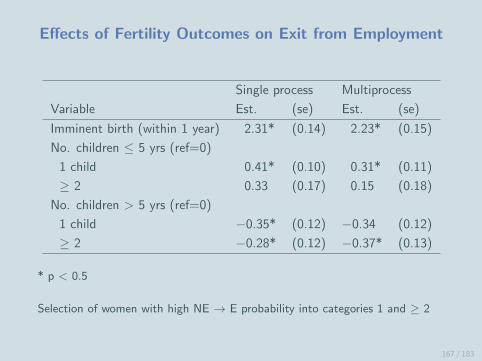
Effects of Fertility Outcomes on Exit from Employment

Single process Multiprocess

Variable Est. (se) Est. (se)

Imminent birth (within 1 year) 2.31* (0.14) 2.23* (0.15)

No. children ≤ 5 yrs (ref=0)

1 child 0.41* (0.10) 0.31* (0.11)

≥ 2 0.33 (0.17) 0.15 (0.18)

No. children > 5 yrs (ref=0)

1 child −0.35* (0.12) −0.34 (0.12)

≥ 2 −0.28* (0.12) −0.37* (0.13)

* p < 0.5

Selection of women with high NE → E probability into categories 1 and ≥ 2

167 / 183

Example: Family Disruption and Children’s Education

Research questions:

What is the association between disruption (due to divorce orpaternal death) and children’s education?

Are the effects of disruption the same across differenteducational transitions?

To what extent can the effect of divorce be explained byselection?

- There may be unobserved factors affecting both parents’dissolution risk and their children’s educational outcomes

Reference: Steele, Sigle-Rushton and Kravdal (2009), Demography.

168 / 183

Strategies for Handling Selection

Exploit longitudinal study designs

- e.g. measures of child wellbeing before divorce, measures ofparental conflict and family environment

Exploit differences across space

- compare children living in places with differences in availabilityof divorce (e.g. US states)

Compare siblings

- Siblings share parents (or parent) but may have differentexposure to disruption

Multiprocess (simultaneous equations) models

169 / 183

SEM for Parental Divorce and Children’s Education

Selection equation: event history model for duration ofmother’s marriage(s)

Sequential probit model for children’s educational transitions(nested within mother)

Equations linked by allowing correlation betweenmother-specific random effects (unmeasured maternalcharacteristics)

Estimated using aML software

170 / 183

Simple Conceptual Model

171 / 183

Sequential Probit Model for Educational Transitions (1)

View educational qualifications as the result of 4 sequentialtransitions:

- Compulsory to lower secondary- Lower to higher secondary (given reached lower sec.)- Higher secondary to Bachelor’s (given higher sec.)- Bachelor’s to postgraduate (given Bachelor’s)

Rather like a discrete-time event history model

Advantages:

- Allow effects of disruption to vary across transitions- Can include children who are too young to have made all

transitions

172 / 183

Sequential Probit Model for Educational Transitions (2)

Transition from education level r for child i of woman j indicated

y(r)ij =1 if child attains level r + 1 and 0 if stops at r .

y(r)ij

∗= β(r)xij + γ(r)zij + λ(r)uj + e

(r)ij , r = 1, . . . , 4

y(r)ij

∗latent propensity underlying y

(r)ij

zij potentially endogenous indicators of family disruption

xij child and mother background characteristics

uj mother-specific random effect

e(r)ij child and transition-specific residual

173 / 183

Unobserved Heterogeneity: Educational Transitions

Effect of mother-level unobservables less important for latertransitions.

174 / 183

Evidence for Selection

Residual correlation between dissolution risk and probability ofcontinuing in education estimated as -0.43 (se=0.02)

Suggests mothers with above-average risk of divorce tend tohave children with below-average chance of remainingeducation

Note that we are controlling only for selection onunobservables at the mother level (i.e. fixed across time)

175 / 183

Effects of Disruption on Transitions in Secondary School

176 / 183

Predicted Probabilities of Continuing Beyond Lower

Secondary (Before and After Allowing for Selection)

177 / 183

Software for multiprocess modelling

Stata

- Responses of same type only: continuous (xtmixed) or binary(xtmelogit)

- Can handle multiple processes in theory, but slow

MLwiN (and runmlwin in Stata)

- Designed for multilevel modelling; multiple levels- Handles mixtures of continuous and binary responses- Markov chain Monte Carlo estimation

Sabre

- Developed for analysis of recurrent events- Handles mixtures of response types; up to 3 processes; 2 levels

aML

- Designed specifically for multilevel multiprocess modelling- Mixtures of response types; multiple processes and levels

178 / 183

discrete -time event history analysis lectures · discrete -time event history analysis lectures...

Documents