discrete mathematics, chapter 3: · pdf fileform. richard mayr (university of edinburgh, uk)...

Discrete Mathematics, Chapter 3:Algorithms

Richard Mayr

University of Edinburgh, UK

Richard Mayr (University of Edinburgh, UK) Discrete Mathematics. Chapter 3 1 / 28

Outline

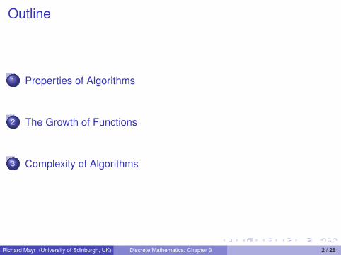
1 Properties of Algorithms

2 The Growth of Functions

3 Complexity of Algorithms


Algorithms (Abu Ja ’far Mohammed Ibin Musa Al-Khowarizmi,

780-850)

DefinitionAn algorithm is a finite set of precise instructions for performing acomputation or for solving a problem.

Example: Describe an algorithm for finding the maximum value in afinite sequence of integers.Description of algorithms in pseudocode:

Intermediate step between English prose and formal coding in aprogramming language.Focus on the fundamental operation of the program, instead ofpeculiarities of a given programming language.Analyze the time required to solve a problem using an algorithm,independent of the actual programming language.


Properties of Algorithms

Input: An algorithm has input values from a specified set.Output: From the input values, the algorithm produces the output

values from a specified set. The output values are thesolution.

Correctness: An algorithm should produce the correct output valuesfor each set of input values.

Finiteness: An algorithm should produce the output after a finitenumber of steps for any input.

Effectiveness: It must be possible to perform each step of thealgorithm correctly and in a finite amount of time.

Generality: The algorithm should work for all problems of the desiredform.


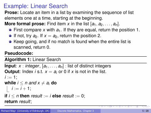
Example: Linear SearchProse: Locate an item in a list by examining the sequence of listelements one at a time, starting at the beginning.More formal prose: Find item x in the list [a1,a2, . . . ,an].

First compare x with a1. If they are equal, return the position 1.If not, try a2. If x = a2, return the position 2.Keep going, and if no match is found when the entire list isscanned, return 0.

Pseudocode:Algorithm 1: Linear SearchInput: x : integer , [a1, . . . ,an] : list of distinct integersOutput: Index i s.t. x = ai or 0 if x is not in the list.i := 1;while i ≤ n and x 6= ai do

i := i + 1;

if i ≤ n then result := i else result := 0;return result ;


Binary Search

Prose description:Assume the input is a list of items in increasing order, and thetarget element to be found.The algorithm begins by comparing the target with the middleelement.

I If the middle element is strictly lower than the target, then thesearch proceeds with the upper half of the list.

I Otherwise, the search proceeds with the lower half of the list(including the middle).

Repeat this process until we have a list of size 1.I If target is equal to the single element in the list, then the position is

returned.I Otherwise, 0 is returned to indicate that the element was not found.


Binary Search

Pseudocode:Algorithm 2: Binary SearchInput: x : integer , [a1, . . . ,an] : strictly increasing list of integersOutput: Index i s.t. x = ai or 0 if x is not in the list.i := 1; // i is the left endpoint of the intervalj := n; // j is the right endpoint of the intervalwhile i < j do

m := b(i + j)/2c;if x > am then i := m + 1 else j := m;

if x = ai then result := i else result := 0;return result ;


Example: Binary SearchFind target 19 in the list: 1 2 3 5 6 7 8 10 12 13 15 16 18 19 20 22

1 The list has 16 elements, so the midpoint is 8. The value in the 8thposition is 10. As 19>10, search is restricted to positions 9-16.1 2 3 5 6 7 8 10 12 13 15 16 18 19 20 22

2 The midpoint of the list (positions 9 through 16) is now the 12thposition with a value of 16. Since 19 > 16, further search isrestricted to the 13th position and above.1 2 3 5 6 7 8 10 12 13 15 16 18 19 20 22

3 The midpoint of the current list is now the 14th position with avalue of 19. Since 19 6> 19, further search is restricted to theportion from the 13th through the 14th positions.1 2 3 5 6 7 8 10 12 13 15 16 18 19 20 22

4 The midpoint of the current list is now the 13th position with avalue of 18. Since 19 > 18, search is restricted to position 14.1 2 3 5 6 7 8 10 12 13 15 16 18 19 20 22

5 Now the list has a single element and the loop ends.Since 19 = 19, the location 14 is returned.


Greedy Algorithms

Optimization problems minimize or maximize some parameterover all possible inputs.Examples of optimization problems:

I Finding a route between two cities with the smallest total mileage.I Determining how to encode messages using the fewest possible

bits.I Finding the fiber links between network nodes using the least

amount of fiber.

Optimization problems can often be solved using a greedyalgorithm, which makes the “best” (by a local criterion) choice ateach step. This does not necessarily produce an optimal solutionto the overall problem, but in many instances, it does.After specifying what the “best choice” at each step is, we try toprove that this approach always produces an optimal solution, orfind a counterexample to show that it does not.


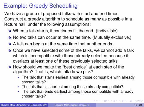
Example: Greedy SchedulingWe have a group of proposed talks with start and end times.Construct a greedy algorithm to schedule as many as possible in alecture hall, under the following assumptions:

When a talk starts, it continues till the end. (Indivisible).No two talks can occur at the same time. (Mutually exclusive.)A talk can begin at the same time that another ends.Once we have selected some of the talks, we cannot add a talkwhich is incompatible with those already selected because itoverlaps at least one of these previously selected talks.How should we make the “best choice” at each step of thealgorithm? That is, which talk do we pick?

I The talk that starts earliest among those compatible with alreadychosen talks?

I The talk that is shortest among those already compatible?I The talk that ends earliest among those compatible with already

chosen talks?


Greedy Scheduling

Picking the shortest talk doesn’t work.But picking the one that ends soonest does work. The algorithm isspecified on the next page.


A Greedy Scheduling AlgorithmAt each step, choose the talks with the earliest ending time among thetalks compatible with those selected.

Algorithm 3: Greedy Scheduling by End TimeInput: s1, s2, . . . , sn start times and e1,e2, . . . ,en end timesOutput: An optimal set S ⊆ 1, . . . ,n of talks to be scheduled.Sort talks by end time and reorder so that e1 ≤ e2 ≤ · · · ≤ enS := ∅;for j := 1 to n do

if Talk j is compatible with S thenS := S ∪ j

return S;

Note: Scheduling problems appear in many applications. Many ofthem (unlike this simple one) are NP-complete and do not allowefficient greedy algorithms.


The Growth of Functions

Given functions f : N→ R or f : R→ R.Analyzing how fast a function grows.

Comparing two functions.Comparing the efficiently of different algorithms that solve thesame problem.Applications in number theory (Chapter 4) and combinatorics(Chapters 6 and 8).


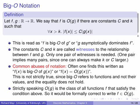
Big-O Notation

DefinitionLet f ,g : R→ R. We say that f is O(g) if there are constants C and ksuch that

∀x > k . |f (x)| ≤ C|g(x)|

This is read as “f is big-O of g” or “g asymptotically dominates f ”.The constants C and k are called witnesses to the relationshipbetween f and g. Only one pair of witnesses is needed. (One pairimplies many pairs, since one can always make k or C larger.)Common abuses of notation: Often one finds this written as“f (x) is big-O of g(x)” or “f (x) = O(g(x))”.This is not strictly true, since big-O refers to functions and not theirvalues, and the equality does not hold.Strictly speaking O(g) is the class of all functions f that satisfy thecondition above. So it would be formally correct to write f ∈ O(g).


Illustration of Big-O Notationf (x) = x2 + 2x + 1, g(x) = x2.f is O(g) witness k = 1 and C = 4.Abusing notation, this is often written as f (x) = x2 + 2x + 1 is O(x2).


Properties of Big-O Notation

If f is O(g) and g is O(f ) then one says that f and g are of thesame order.If f is O(g) and h(x) ≥ g(x) for all positive real numbers x then fis O(h).The O-notation describes upper bounds on how fast functionsgrow. E.g., f (x) = x2 + 3x is O(x2) but also O(x3), etc.Often one looks for a simple function g that is as small aspossible such that still f is O(g).(The word ‘simple’ is important, since trivially f is O(f ).)


Example

Bounds on functions. Prove thatf (x) = anxn + an−1xn−1 + · · ·+ a1x + a0 is O(xn).1 + 2 + · · ·+ n is O(n2).n! = 1× 2× · · · × n is O(nn).log(n!) is O(n log(n)).


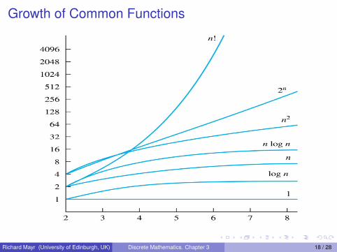
Growth of Common Functions


Useful Big-O Estimates

If d > c > 1, then nc is O(nd ), but nd is not O(nc).If b > 1 and c and d are positive, then (logb n)c is O(nd ), but nd isnot O((logb n)c).If b > 1 and d is positive, then nd is O(bn), but bn is not O(nd ).If c > b > 1, then bn is O(cn), but cn is not O(bn).If f1(x) is O(g1(x)) and f2(x) is O(g2(x)) then (f1 + f2)(x) isO(max(|g1(x)|, |g2(x)|)).If f1 is O(g1) and f2 is O(g2) then (f1 f2) is O(g1 g2).

Note: These estimates are very important for analyzing algorithms.Suppose that g(n) = 5n2 + 7n− 3 and f is a very complex function thatyou cannot determine exactly, but you know that f is O(n3).Then you can still derive that n · f (n) is O(n4) and g(f (n)) is O(n6).


Big-Omega Notation

DefinitionLet f ,g : R→ R. We say that f is Ω(g) if there are constants C and ksuch that

∀x > k . |f (x)| ≥ C|g(x)|

This is read as “f is big-Omega of g”.The constants C and k are called witnesses to the relationshipbetween f and g.Big-O gives an upper bound on the growth of a function, whileBig-Omega gives a lower bound. Big-Omega tells us that afunction grows at least as fast as another.Similar abuse of notation as for big-O.f is Ω(g) if and only if g is O(f ).(Prove this by using the definitions of O and Ω.)


Big-Theta Notation

DefinitionLet f ,g : R→ R. We say that f is Θ(g) if f is O(g) and f is Ω(g).

We say that “f is big-Theta of g” and also that “f is of order g” andalso that “f and g are of the same order”.f is Θ(g) if and only if there exists constants C1, C2 and k suchthat C1g(x) < f (x) < C2g(x) if x > k . This follows from thedefinitions of big-O and big-Omega.


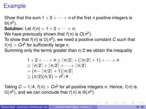
Example

Show that the sum 1 + 2 + · · ·+ n of the first n positive integers isΘ(n2).Solution: Let f (n) = 1 + 2 + · · ·+ n.We have previously shown that f (n) is O(n2).To show that f (n) is Ω(n2), we need a positive constant C such thatf (n) > Cn2 for sufficiently large n.Summing only the terms greater than n/2 we obtain the inequality

1 + 2 + · · ·+ n ≥ dn/2e+ (dn/2e+ 1) + · · ·+ n≥ dn/2e+ dn/2e+ · · ·+ dn/2e= (n − dn/2e+ 1)dn/2e≥ (n/2)(n/2) = n2/4

Taking C = 1/4, f (n) > Cn2 for all positive integers n. Hence, f (n) isΩ(n2), and we can conclude that f (n) is Θ(n2).


Complexity of AlgorithmsGiven an algorithm, how efficient is this algorithm for solving aproblem given input of a particular size?

I How much time does this algorithm use to solve a problem?I How much computer memory does this algorithm use to solve a

problem?

We measure time complexity in terms of the number of operationsan algorithm uses and use big-O and big-Theta notation toestimate the time complexity.Compare the efficiency of different algorithms for the sameproblem.We focus on the worst-case time complexity of an algorithm.Derive an upper bound on the number of operations an algorithmuses to solve a problem with input of a particular size.(As opposed to the average-case complexity.)Here: Ignore implementation details and hardware properties.−→ See courses on algorithms and complexity.


Worst-Case Complexity of Linear SearchAlgorithm 4: Linear SearchInput: x : integer , [a1, . . . ,an] : list of distinct integersOutput: Index i s.t. x = ai or 0 if x is not in the list.i := 1;while i ≤ n and x 6= ai do

i := i + 1;

if i ≤ n then result := i else result := 0;return result ;

Count the number of comparisons.At each step two comparisons are made; i ≤ n and x 6= ai .To end the loop, one comparison i ≤ n is made.After the loop, one more i ≤ n comparison is made.

If x = ai , 2i + 1 comparisons are used. If x is not on the list, 2n + 1comparisons are made and then an additional comparison is used toexit the loop. So, in the worst case 2n + 2 comparisons are made.Hence, the complexity is Θ(n).


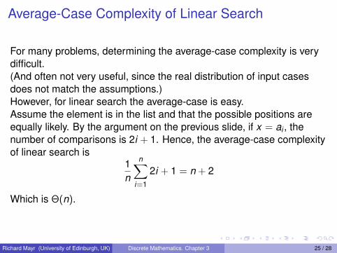
Average-Case Complexity of Linear Search

For many problems, determining the average-case complexity is verydifficult.(And often not very useful, since the real distribution of input casesdoes not match the assumptions.)However, for linear search the average-case is easy.Assume the element is in the list and that the possible positions areequally likely. By the argument on the previous slide, if x = ai , thenumber of comparisons is 2i + 1. Hence, the average-case complexityof linear search is

1n

n∑i=1

2i + 1 = n + 2

Which is Θ(n).


Worst-Case Complexity of Binary SearchAlgorithm 5: Binary SearchInput: x : integer , [a1, . . . ,an] : strictly increasing list of integersOutput: Index i s.t. x = ai or 0 if x is not in the list.i := 1; // i is the left endpoint of the intervalj := n; // j is the right endpoint of the intervalwhile i < j do

m := b(i + j)/2c;if x > am then i := m + 1 else j := m;

if x = ai then result := i else result := 0;return result ;

Assume (for simplicity) n = 2k elements. Note that k = log n.Two comparisons are made at each stage; i < j , and x > am.At the first iteration the size of the list is 2k and after the first iteration it is2k−1. Then 2k−2 and so on until the size of the list is 21 = 2.At the last step, a comparison tells us that the size of the list is the size is20 = 1 and the element is compared with the single remaining element.Hence, at most 2k + 2 = 2 log n + 2 comparisons are made. Θ(log n).


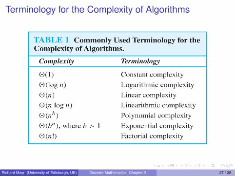
Terminology for the Complexity of Algorithms


Further topics

See courses on algorithms and complexity forSpace vs. time complexityIntractable problemsComplexity classes: E.g., P, NP, PSPACE, EXPTIME, EXPSPACE,etc.Undecidable problems and the limits of algorithms.


discrete mathematics, chapter 3: · pdf fileform. richard mayr (university of edinburgh, uk)...

Documents