discovering multi-label temporal patterns in sequence databases

Information Sciences 181 (2011) 398–418

Contents lists available at ScienceDirect

Information Sciences

journal homepage: www.elsevier .com/locate / ins

Discovering multi-label temporal patterns in sequence databases

Yen-Liang Chen a,⇑, Shin-Yi Wu b, Yu-Cheng Wang a

a Department of Information Management, National Central University, Chung-Li 320, Taiwan, ROCb Industrial Technology Research Institute, Hsinchu 320, Taiwan, ROC

a r t i c l e i n f o a b s t r a c t

Article history:Received 4 July 2009Received in revised form 3 September 2010Accepted 12 September 2010

Keywords:Sequential patternsPoint-based event sequenceInterval-based event sequenceTemporal patterns

0020-0255/$ - see front matter � 2010 Elsevier Incdoi:10.1016/j.ins.2010.09.024

⇑ Corresponding author. Tel.: +886 3 4267266; faE-mail address: [email protected] (Y.-L. Ch

Sequential pattern mining is one of the most important data mining techniques. Previousresearch on mining sequential patterns discovered patterns from point-based event data,interval-based event data, and hybrid event data. In many real life applications, however,an event may involve many statuses; it might not occur only at one certain point in time orover a period of time. In this work, we propose a generalized representation of temporalevents. We treat events as multi-label events with many statuses, and introduce an algo-rithm called MLTPM to discover multi-label temporal patterns from temporal databases.The experimental results show that the efficiency and scalability of the MLTPM algorithmare satisfactory. We also discuss interesting multi-label temporal patterns discoveredwhen MLTPM was applied to historical Nasdaq data.

� 2010 Elsevier Inc. All rights reserved.

1. Introduction

Data mining (DM) extracts implicit, previously unknown, and potentially useful information from databases. It has beensuccessfully used in many applications, such as risk analysis, financial analysis, customer relationship management, churnprediction, fraud detection, and so on. Many data mining approaches have been proposed to discover knowledge from dif-ferent types of data. Sequential pattern mining is one of the most important techniques in the data mining research field.

The sequential pattern mining problem was first introduced in the mid-1990s [4]. A typical example of a sequential pat-tern is a customer who, after buying a computer, returns to buy a scanner and a microphone. In this example, the sequencedata is nothing but a sequence of events (items) that happen chronologically, and the pattern tells us which items werebought and in what order.

According to the classification scheme proposed by Wu and Chen [38], traditional sequential pattern mining methods canbe classified into three categories: (1) point-based methods, which discover patterns from point-based event sequences, (2)interval-based methods, which discover patterns from interval-based event sequences, and (3) hybrid-based methods, whichdiscover patterns from hybrid event sequences.

The first type assumes that events are point-based events, which is the common assumption adopted by most previoussequential pattern mining studies. An event is viewed as something that occurs at a certain point in time. For example, inanalyzing web traversal behaviors, if we record when users visit pages but not how long they stay, then every visit canbe treated as a point-based event. In the past, research on web usage mining has investigated how we can transform users’browsing data into point-based sequence data through data preprocessing techniques, and how interesting web traversalbehaviors can be discovered by applying sequential pattern mining methods [10–13,32,33,40].

In many practical situations, however, events cannot be represented as points. In the web traversal application example, avisit becomes an interval event if we record when the page is visited and how long the user stays. Therefore, some previous

. All rights reserved.

x: +886 3 4254604.en).

http://dx.doi.org/10.1016/j.ins.2010.09.024

mailto:[email protected]

http://dx.doi.org/10.1016/j.ins.2010.09.024

http://www.sciencedirect.com/science/journal/00200255

http://www.elsevier.com/locate/ins

Fig. 1. The statuses that occur during the flu.

Y.-L. Chen et al. / Information Sciences 181 (2011) 398–418 399

research extended the sequential pattern mining problem to include interval-based events [19,39]. When events are inter-vals, an event can be described with three major characteristics: event name, event starting time, and event ending time. Theresearch on mining temporal patterns from interval-based events attempted to find the temporal relationships betweenthese interval events. For example, in a hospital-related application, a temporal pattern may be that patients frequently starta fever when they start to cough and these symptoms all occur when they catch the flu.

In some applications, however, events are neither purely point-based nor purely interval-based; they are hybrid events.For example, phenomena in meteorology can be treated as hybrid events. Thunder and lightning are point-based events,while rain, snow, and sunshine are interval-based events. One common meteorological hybrid temporal pattern is ‘‘thunder(point-based event) occurred after a lightning strike, and they both occurred during rain (interval-based event)”. This pat-tern, consisting of point- and interval-based events, is called a hybrid temporal pattern. The research on mining temporal pat-terns from hybrid events attempted to find the temporal relationships between these hybrid events.

As discussed above, there are three types of sequential pattern mining models, categorized by the type of events con-tained in the sequences. All three models can be summarized by a simple observation: point events are events with one label,interval events are events with two labels, and hybrid events have one or two labels. This work proposes the multi-labelmodel of sequential pattern mining. The model is more capable of describing sequence data that could not be representedby previous models. In the following, we introduce the multi-label model.

In some applications, an event can have many different statuses; we call these events multi-label events. For example, asshown in Fig. 1, when a patient gets the flu (event start), he may have some symptoms (statuses), like a sore throat, runnynose, and a fever. He may be treated by a doctor (status), and at the same time, he may have another disease (another event),like pneumonia. During the entire ‘‘flu” period, the situation may change involving different statuses in the same event ordifferent events. The evolution of these statuses, whether in the same or different events, may have some associations; mul-ti-label temporal pattern mining attempts to discover the status relationships among these events.

There are other potential applications of multi-label temporal pattern mining. In traditional web management, the weblog only records when a visitor visits a page. Nowadays, it is possible to record more information in the web log, such as theactions performed on a visited page, due to the Ajax technology [15]. Ajax is a group of inter-related web development tech-niques used for creating interactive web applications by exchanging small amounts of data with the server ‘‘behind thescenes”. This means the entire web page does not have to be reloaded each time the user performs an action [1]. By recordingusers’ actions in Ajax applications, we can collect information about what actions are performed by users on which pages.Fig. 2 shows a possible sequence with multi-actions. From this kind of sequence data, we may find a pattern like the figure onthe right. It means a user browsed a ‘‘member register” page a (astart) and clicked a button (a1) to check if his user name wasavailable. Then he clicked a link (a2) to obtain some information from the popup window (bstart), closed it (bend), and finally,he clicked the submit button (aend) to finish the registration process.

The discussions above indicate that multi-label sequence data exist in practice. Unfortunately, since traditional modelsdid not consider multi-label sequence data, they treated multi-label sequence data as either point-based or interval-basedevent data. This means a large portion of temporal relationships were unused when discovering knowledge, and as a result,the patterns discovered are incomplete and partial. This research gap suggests that traditional sequential pattern miningapproaches should be extended to deal with multi-label sequence data.

Fig. 2. A multi-label web sequence data and pattern.

400 Y.-L. Chen et al. / Information Sciences 181 (2011) 398–418

This paper proposes an algorithm, called MLTPM, for discovering multi-label temporal patterns from multi-label sequencedata, called multi-label temporal pattern mining. The paper is organized as follows. Section 2 reviews the related research onsequential pattern mining and temporal pattern mining. Section 3 formally defines the problem of multi-label temporalpattern mining. In Section 4, we focus on the algorithm’s design. Section 5 discusses experiments that evaluate thealgorithm’s performance using several previous algorithms, synthetic data sets, and real financial data sets. Finally, wediscuss our conclusions and provide some suggestions for future work.

2. Related work

Data mining with temporal sequences has attracted the attention of many researchers. Different technologies have beenused to deal with temporal sequences, including sequential pattern mining [4,16,18,27,31,34,43], association rules [19,35],and classification [25]. Sequential pattern mining was the research field that attracted most scholars’ attention. There aretwo main research issues in sequential pattern mining. The first is developing efficient algorithms, like FreeSpan [18],PrefixSpan [31], GSP [34], SPADE [43], etc. The second research issue is the mining of other time-related patterns, such asfrequent episodes [28], similar patterns [3,26], typical patterns [20], traversal patterns [10,12], multidimensional patterns[42], constraint-based sequential patterns [7,30,37], time-interval sequential patterns [8,22,23,41], fuzzy sequential patterns[9,14,21], spatial–temporal patterns [6,24], trajectory patterns [17,24], patterns in data stream [29], etc.

Most previous studies [4,18,31,34,43] on temporal sequences viewed an item as a point-based event that occurs at a cer-tain point in time. As mentioned previously, an example of a sequential pattern could be a customer who buys a computer,then returns to buy a scanner and a printer. In many cases, however, events are better suited as intervals, rather than specifictime points. For example, an event like ‘‘a user browses a web page” does not happen at a certain time, but over a period oftime.

Because of the limitations of point-based event representation, some studies investigated interval-based events in spe-cific domains and applications. In [19], Hoppner and Klawonn proposed a method of uncovering informative rules in inter-val-based event sequences. The temporal containment relationships between interval-based events were explored in [36].Based on Allen’s work [5], which classifies the relationship between two interval-based events into 13 temporal relation-ships, Kam and Fu [22] proposed an Apriori-like approach to discover frequent temporal patterns from interval-based events,which can reveal the temporal relationships between events. For example, we may find a pattern like ‘‘event A occurs duringthe duration of event B.” Although Kam and Fu’s work is impressive, the major weakness of their approach is that the pat-terns generated may have ambiguous semantics.

More recently, Wu and Chen [39] proposed another extended method to uncover relationships among interval-basedevents without encountering the ambiguity problem in Kam and Fu’s work. In Wu and Chen’s study, the start times andend times of the interval-based events are stored in temporal databases. This method is able to discover the exact relation-ships between two interval-based events without ambiguities. Additionally, Wu and Chen [38] provided another algorithmto deal with hybrid events, which consists of point-based events and interval-based events.

Here, it should be noted that in many real life applications, events often have more than two statuses, not just ‘‘happen”,‘‘start”, and ‘‘end”, and these statuses may reveal important information. The event structures proposed in previous researchwere unable to present multi-status events. In order to resolve this problem, this work introduces the multi-label eventsmodel, where every event is represented by labels that stand for different statuses.

In this work, we compare our proposed algorithm with several methods, including GSP [34], PrefixSpan [31], TPrefixSpan[39], and HTPM [38]. GSP [34] is an Apriori-like algorithm, and it follows the candidate-generation-and-test process. Prefix-Span is a pattern-growth method, and PrefixSpan [31] can reduce the time spent scanning a database by avoiding the can-didate generation step. GSP [34] and PrefixSpan [31] are both traditional methods that discover patterns from point-basedevent data sets. Another algorithm, TPrefixSpan [39], is extended from PrefixSpan [31] to discover patterns from interval-based events. Finally, HTPM [38] is designed to uncover patterns from hybrid event data sets. HTPM [38] is similar to thetraditional candidate-generation-and-test process, but it generates patterns by joining the patterns’ occurrence recordsand calculates the patterns’ support by checking the occurrence records.

3. Problem definition

To incorporate the concept of multi-label temporal mining, we recorded not only events’ occurrence times, but also theirstatuses (labels). For example, Table 1 shows a sequence database D containing three fields: sequence ID, item (event status),and time. Based on these fields, we describe how multi-label temporal sequences and patterns are represented and definethe problem of mining multi-label temporal patterns.

Definition 1 (Multi-label item). Let event types 1,2, . . ., and u be all the event types in temporal database D and let

Li ¼ li1; li2; . . . ; lit

n obe the set of all labels for event type i. Since an event type may have multiple occurrences in a sequence

where states change over time, we use a multi-label item to refer to the state of an event type’s specific occurrence. Thus, amulti-label item has three related attributes: its event type, the occurrence number of the event type, and its label index.Accordingly, we define the following notations for a multi-label item it:

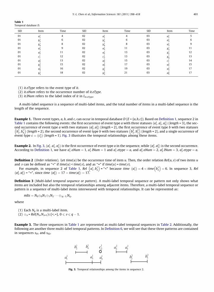
Table 1Temporal database D.

SID Item Time SID Item Time SID Item Time

01 a11

4 02 a11

4 03 a11

5

01 b12

6 02 b12

6 03 a13

6

01 b14

8 02 b14

8 03 a13

9

01 a13

9 02 a13

11 03 b13

11

01 a12

11 02 a12

13 03 b12

12

01 c11

12 02 c12

13 03 b14

13

01 a22

13 02 a22

15 03 c11

14

01 b22

15 02 a23

17 03 a21

15

01 a24

16 02 b22

19 03 a23

17

01 b23

18 02 b23

21 03 a25

17


(1) it.eType refers to the event type of it.(2) it.oNum refers to the occurrence number of it.eType.(3) it.lNum refers to the label index of it in Lit.eType.

A multi-label sequence is a sequence of multi-label items, and the total number of items in a multi-label sequence is thelength of the sequence.

Example 1. Three event types, a, b, and c, can occur in temporal database D (E = {a,b,c}). Based on Definition 1, sequence 2 inTable 1 contains the following events: the first occurrence of event type a with three statuses a1

1; a13; a

12

� �(length = 3), the sec-

ond occurrence of event type a with two statuses a22; a

23

� �(length = 2), the first occurrence of event type b with two statuses

b12; b

14

� �(length = 2), the second occurrence of event type b with two statuses b2

2; b23

� �(length = 2), and a single occurrence of

event type c ¼ c12

� �(length = 1). Fig. 3 illustrates the temporal relationships among these items.

Example 2. In Fig. 3, a11; a

13; a

12

� �is the first occurrence of event type a in the sequence, while a2

2; a23

� �is the second occurrence.

According to Definition 1, we have a11:oNum ¼ 1, a1

1:lNum ¼ 1 and a11:etype ¼ a, and a2

3:oNum ¼ 2, a23:lNum ¼ 3, a2

3:etype ¼ a.

Definition 2 (Order relations). Let time(u) be the occurrence time of item u. Then, the order relation Rel(u,v) of two items uand v can be defined as ‘‘<” if time(u) < time(v), and as ‘‘=” if time(u) = time(v).

For example, in sequence 2 of Table 1, Rel a11; b

12

� �= ‘‘<” because time a1

1

� �¼ 4 < time b1

2

� �¼ 6. In sequence 3, Rel

a23; a

25

� �= ‘‘=”, since time a2

3

� �¼ 17 ¼ timeða2

5Þ ¼ 17.

Definition 3 (Multi-label temporal sequence or pattern). A multi-label temporal sequence or pattern not only shows whatitems are included but also the temporal relationships among adjacent items. Therefore, a multi-label temporal sequence orpattern is a sequence of multi-label items interweaved with temporal relationships. It can be represented as:

mlts ¼ N0�0N1�1N2 � � � �ðq�1ÞNq;

where

(1) Each Np is a multi-label item.(2) �v = Rel(Nv,Nv+1)2{<,=}, 0 6 v 6 q � 1.

Example 3. The three sequences in Table 1 are represented as multi-label temporal sequences in Table 2. Additionally, thefollowing are another three multi-label temporal patterns. In Definition 6, we will see that these three patterns are containedin sequences s01 and s02.

11a 1

2a13a

14b1

2b 22a 2

3a

23b2

2b

12c

Fig. 3. Temporal relationships among the items in sequence 2.

Table 2Formal representation of multi-label temporal sequences in D.

Multi-label temporal sequence Illustration

s01 a11 < b1

2 < b14 < a1

3 < a12 < c1

1 < a22 < b2

2 < a24 < b2

3

s02 a11 < b1

2 < b14 < a1

3 < a12 ¼ c1

2 < a22 < a2

3 < b22 < b2

3

s03 a11 < a1

3 < a13 < b1

3 < b12 < b1

4 < c11 < a2

1 < a23 ¼ a2

5


(1) p1 ¼ a11 < a1

2.(2) p2 ¼ a1

1 < a13 < a1

2 < a22.

(3) p3 ¼ a11 < b1

2 < a13 < b2

2 < b23.

Definition 4 (Arrangement of items). In a multi-label sequence or a multi-label temporal pattern, item u must be placedbefore item v based on the following conditions:

(1) time(u) < time(v).(2) If time(u) = time(v), but u’s event type alphabetically precedes that of v.(3) If time(u) = time(v) and u is the same event type as v, but u’s label number is less than v’s.(4) If the above criteria are all tied, but u’s occurrence number is less than v’s.

Example 4. In Fig. 4, there are three multi-label event types with a total of six items in pattern mltp. Based on Definition 4,mltp ¼ a1

1 < a12 ¼ a2

2 ¼ a13 ¼ b1

1 < b12, where a1

1 < a12 and b1

1 < b12 are arranged according to condition 1, a1

3 ¼ b11 is arranged

according to condition 2, a22 ¼ a1

3 is arranged according to condition 3, and a12 ¼ a2

2 is arranged according to condition 4.When checking if a pattern appears in a sequence, we usually have to determine the relation between the two events.

Therefore, we introduce the small operation.

Definition 5 (Small operation). Function Small(�r,�r+1, . . . ,�q), where �i 2 {<,=}, will output ‘‘<” if any �i, r 6 i 6 q, is ‘‘<”.Otherwise, the output of Small is ‘‘=”.

For example, if mltp ¼ a11 < b1

2 < a12 < a1

3 ¼ b13 ¼ c1

1

� �, then Rel a1

2; c11

� �¼ Smallð<;¼;¼Þ = ‘‘<”, and Rel a1

3; c11

� �=

Small(=,=) = ‘‘=”.

Definition 6 (Containment). Suppose there are two multi-label temporal sequences, mlts = (s1 �1 s2 �2 � � � �n�1 sn) andmltp = (p1 �1 p2 �2 � � � �r�1 pr), r 6 n. Then, mltp is contained in mlts, denoted as mltp # mlts, if there are r indices in mlts,denoted as 1 6w1 6 w2 6 � � � 6 wr 6 n, satisfying the conditions below:

(1) Type equivalence: pa.eType = swa.eType for 1 6 a 6 r.

(2) Label equivalence: pa.lNum = swa.lNum for 1 6 a 6 r.

time

11a 1

312 , aa

11b 1

2b

22a

12

11

13

22

12

11 bbaaaamltp <===<=

Fig. 4. An example that shows how items are ordered.


(3) Occurrence number agreement: If pa.eType = pb.eType and pa.oNum = pb.oNum, 1 6 a, b 6 r, then swa.eType = swb

.eTypeand swa

.oNum = swb.oNum.

(4) Same label ordering: �i ¼ Smallð�wi; . . . ;�wiþ1�1Þ, for i = 1 to r � 1.

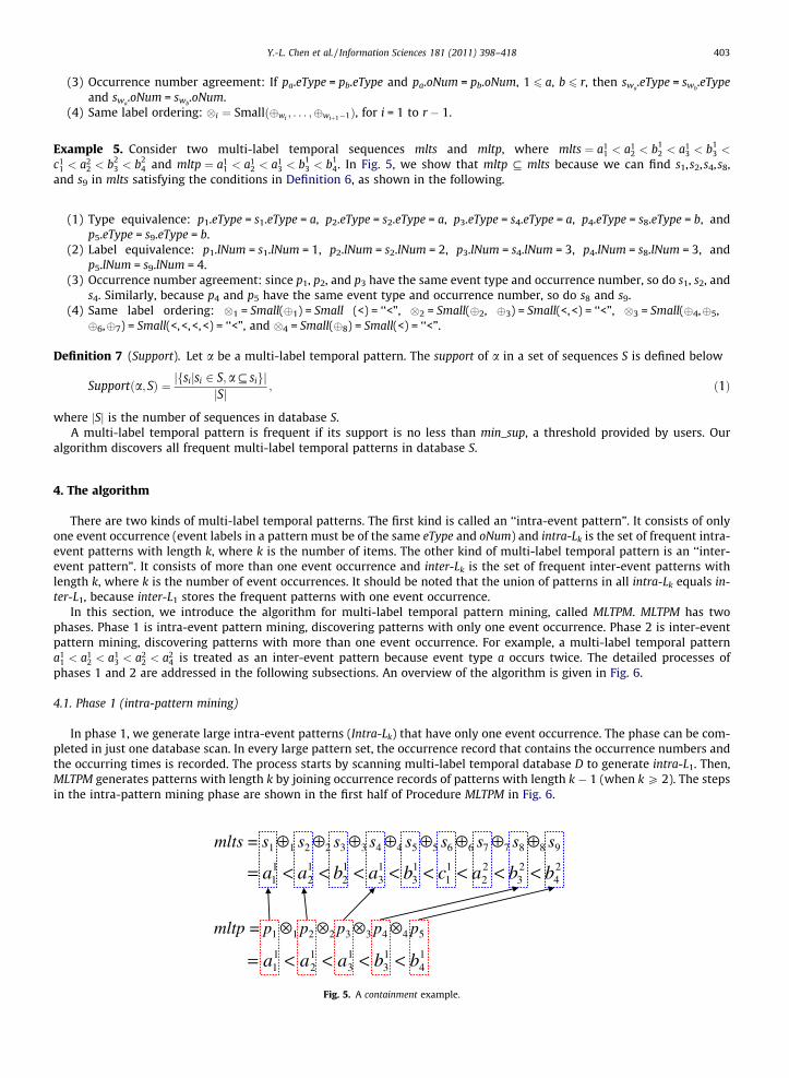
Example 5. Consider two multi-label temporal sequences mlts and mltp, where mlts ¼ a11 < a1

2 < b12 < a1

3 < b13 <

c11 < a2

2 < b23 < b2

4 and mltp ¼ a11 < a1

2 < a13 < b1

3 < b14. In Fig. 5, we show that mltp # mlts because we can find s1,s2,s4,s8,

and s9 in mlts satisfying the conditions in Definition 6, as shown in the following.

(1) Type equivalence: p1.eType = s1.eType = a, p2.eType = s2.eType = a, p3.eType = s4.eType = a, p4.eType = s8.eType = b, and
p5.eType = s9.eType = b.
(2) Label equivalence: p1.lNum = s1.lNum = 1, p2.lNum = s2.lNum = 2, p3.lNum = s4.lNum = 3, p4.lNum = s8.lNum = 3, andp5.lNum = s9.lNum = 4.

(3) Occurrence number agreement: since p1, p2, and p3 have the same event type and occurrence number, so do s1, s2, ands4. Similarly, because p4 and p5 have the same event type and occurrence number, so do s8 and s9.

(4) Same label ordering: �1 = Small(�1) = Small (<) = ‘‘<”, �2 = Small(�2, �3) = Small(<,<) = ‘‘<”, �3 = Small(�4,�5,�6,�7) = Small(<,<,<,<) = ‘‘<”, and �4 = Small(�8) = Small(<) = ‘‘<”.

Definition 7 (Support). Let a be a multi-label temporal pattern. The support of a in a set of sequences S is defined below

Supportða; SÞ ¼ jfsijsi 2 S;a # sigjjSj ; ð1Þ

where jSj is the number of sequences in database S.A multi-label temporal pattern is frequent if its support is no less than min_sup, a threshold provided by users. Our

algorithm discovers all frequent multi-label temporal patterns in database S.

4. The algorithm

There are two kinds of multi-label temporal patterns. The first kind is called an ‘‘intra-event pattern”. It consists of onlyone event occurrence (event labels in a pattern must be of the same eType and oNum) and intra-Lk is the set of frequent intra-event patterns with length k, where k is the number of items. The other kind of multi-label temporal pattern is an ‘‘inter-event pattern”. It consists of more than one event occurrence and inter-Lk is the set of frequent inter-event patterns withlength k, where k is the number of event occurrences. It should be noted that the union of patterns in all intra-Lk equals in-ter-L1, because inter-L1 stores the frequent patterns with one event occurrence.

In this section, we introduce the algorithm for multi-label temporal pattern mining, called MLTPM. MLTPM has twophases. Phase 1 is intra-event pattern mining, discovering patterns with only one event occurrence. Phase 2 is inter-eventpattern mining, discovering patterns with more than one event occurrence. For example, a multi-label temporal patterna1

1 < a12 < a1

3 < a22 < a2

4 is treated as an inter-event pattern because event type a occurs twice. The detailed processes ofphases 1 and 2 are addressed in the following subsections. An overview of the algorithm is given in Fig. 6.

4.1. Phase 1 (intra-pattern mining)

In phase 1, we generate large intra-event patterns (Intra-Lk) that have only one event occurrence. The phase can be com-pleted in just one database scan. In every large pattern set, the occurrence record that contains the occurrence numbers andthe occurring times is recorded. The process starts by scanning multi-label temporal database D to generate intra-L1. Then,MLTPM generates patterns with length k by joining occurrence records of patterns with length k � 1 (when k P 2). The stepsin the intra-pattern mining phase are shown in the first half of Procedure MLTPM in Fig. 6.

mlts = s1 ⊕1 s2 ⊕2 s3 ⊕3 s4 ⊕4 s5 ⊕5 s6 ⊕6 s7 ⊕7 s8 ⊕8 s9

mltp = p1 ⊗1 p2 ⊗2 p3 ⊗3 p4 ⊗4 p5

24

23

22

11

13

13

12

12

11 bbacbabaa <<<<<<<<=

14

13

13

12

11 bbaaa <<<<=

Fig. 5. A containment example.

Fig. 6. The MLTPM algorithm.


Although the high-level view of the intra-event pattern mining process seems similar to Apriori [4], there are some sig-nificant differences:

(1) Database scan: Apriori needs multiple database scans, while the intra-event mining process of MLTPM (intra-MLTPM)needs only one database scan to obtain patterns’ occurrence records.

(2) Candidate generation: Apriori generates candidates with length k by joining all pairs of (k � 1)-patterns with the samefirst (k � 2) items, while intra-MLTPM must also take into account whether they have the same occurrence records.

(3) Frequency computing: Apriori computes patterns’ frequencies by scanning the original database, while intra-MLTPMobtains patterns’ frequencies by checking the occurrence records without any additional computations.

After explaining the differences between Apriori and intra-MLTPM, we now describe how intra-MLTPM progresses. Fromthe multi-label temporal database D shown in Table 1, we have the event set E = {a,b,c}. The subroutine GenIntraL1 scans

database D once, and obtains large 1 intra-event pattern set intra-L1 ¼ a11; a

12; a

13; b

12; b

13; b

14; c

11

n o. Each pattern in intra-L1 is

associated with an occurrence record in Table 3. MLTPM maintains the occurrence record for each pattern in order to gen-erate other patterns in the next step. An occurrence record’s format is defined below.

Definition 8 (Occurrence record). Occurrence records store patterns’ occurrence times in each sequence. Since a multi-labeltemporal pattern mltp may appear in a sequence si several times, we represent all matching combinations for a multi-labeltemporal pattern mltp in sequence si as match(mltp,si). Suppose there are n sequences in the temporal database D. Theoccurrence record of mltp = (p1 �1 p2 �2 � � � �(k�1) pk), denoted as mltp.OR, is defined below:

mltp:OR ¼ fmatchðmltp; s1Þ;matchðmltp; s2; . . . ;matchðmltp; snÞg; wherematchðmltp; siÞ ¼ ½hðoNum1; t1;1Þ; ðoNum1; t1;2Þ; . . . ; ðoNum1; t1;kÞi;

hðoNum2; t2;1Þ; ðoNum2; t2;2Þ; . . . ; ðoNum2; t2;kÞi;. . .

hðoNumx; tx;1Þ; ðoNumx; tx;2Þ; . . . ; ðoNumx; tx;kÞi�;

Table 31-Intra-event patterns (intra-L1) with occurrence records.

Pattern Index Occurring time Pattern Index Occurring time

a11

s1 h(1,4)i b12

s1 h(1,6)i, h(2,15)is2 h(1,4)i s2 h(1,6)i, h(2,19)is3 h(1,5)i, h(2,15)i s3 h(1,12)i

a12

s1 h(1,11)i, h(2,13)i b13

s1 h(2,18)is2 h(1,13)i, h(2,15)i s2 h(2,21)i

a13

s1 h(1,9)i s3 h(1,11)is2 h(1,11)i, h(2,17)i b1

4s1 h(1,8)i

s3 h(1,6)i, h(1,9)i, h(2,17)i s2 h(1,8)i

c11

s1 h(1,12)i s3 h(1,13)is3 h(1,14)i

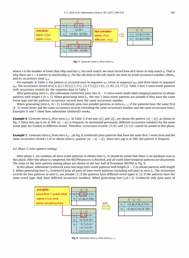
Fig. 7. Generate intra-L2 from intra-L1.


where x is the number of times that mltp matches si. For each match, we must record how all k items in mltp match si. That iswhy there are x � k entries in match(mltp,si). For the vth item in the uth match, we store its event occurence number, oNumu,and its occurrence time tu,v.

For example, in Table 3, the pattern a13 occurred once in sequence s01, twice in sequence s02, and three times in sequence

s03. The occurrence record of a13 is {[h(1,9)i], [h(1,11)i, h(2,17)i], [h(1,6)i, h(1,9)i, h(2,17)i]}. Table 3 lists 1-intra-event patterns

with occurrence records for the sequence data in Table 1.After generating intra-L1, the subroutine GenIntraLk joins two (k � 1)-intra-event multi-label temporal patterns to obtain

patterns with length k (k P 2). When generating intra-L2, the two 1-intra-event patterns are joinable if they have the sameevent type and the patterns’ occurrence records have the same occurrence number.

When generating intra-Lk (k > 2), GenIntraLk joins two joinable patterns in intra-L(k�1) if the patterns have the same first(k�2)-event items and the same occurrence records (including the same occurrence number and the same occurrence time).Examples 6 and 7 show how subroutine GenIntraLk works.

Example 6 (Generate intra-L2 from intra-L1). In Table 3, if we join a11

� �and a1

2

� �, we obtain the pattern a1

1 < a12

� �, as shown in

Fig. 7. Since min_sup is set at 50% a11 < a1

2

� �is frequent. As mentioned previously, different occurrence numbers for the same

event type are treated as different events. Therefore, occurrence records h(1,4)i and h(2,13)i cannot be joined in this phase.

Example 7. Generate intra-Lk from intra-L(k�1)In Fig. 8, GenIntraLk joins patterns that have the same first 1 event item and thesame occurrence record (1,4) to obtain intra-L3 pattern a1

1 < a13 < a1

2

� �. Since min_sup is at 50%, the pattern is frequent.

4.2. Phase 2 (inter-pattern mining)

After phase 1, we combine all intra-event patterns to obtain inter-L1. It should be noted that there is no database scan inthis phase. After this phase is completed, the MLTPM process is finished, and all multi-label temporal patterns are discovered.The steps to the inter-pattern mining phase are shown in the last half of Procedure MLTPM in Fig. 6.

In this phase, subroutine GenInterLk joins two large inter-event patterns with length (k � 1) to obtain patterns with lengthk. When generating inter-L2, GenInterLk joins all pairs of inter-event patterns (including self-join) in inter-L1. The occurrencerecords for two patterns in inter-L1 are joinable (1) if the patterns have different event types or (2) if the patterns have thesame event type, they have different occurrence numbers. When generating inter-Lk(k > 2), GenInterLk only joins pairs of

Fig. 8. Generate intra-Lk from intra-L(k�1).


inter-event patterns in inter-L(k�1) that have the same first (k � 2) events. (They must have the same occurrence number andthe same occurrence time.) Furthermore, two occurrence records for patterns in inter-L(k�1) are joinable (1) if they have dif-ferent last event types or (2) if they have the same last event type, they have different occurrence numbers. Examples 8–10show the details of the inter-pattern generation process.

Example 8 (Generating inter-L2 from inter-L1). In Fig. 9, the two inter-L1 patterns a11 < a1

2

� �and b1

2 < b13

� �have different

event types, so they are joinable. They produce the inter-L2 patterns.

Example 9 (Generating inter-L2 from inter-L1). In Fig. 10, although the two inter-L1 patterns b12

� �and b1

2 < b13

� �have the

same event type, their occurrence records have different occurrence numbers. Therefore, we join occurrence recordh(1,6)i with h(2,15), (2,18)i to produce the inter-event pattern.

Fig. 9. Generating inter-L2 from inter-L1.

Fig. 10. Generating inter-L2 from inter-L1.

Fig. 11. Generating inter-Lk from inter-L(k�1).


Example 10 (Generating inter-Lk from inter-L(k�1)). In Fig. 11, the two inter-L2 patterns are joinable because:

(1) They have the same first 1 event, a11 < a1

2, and the same occurrence record, h(1,4), (1,11)i.(2) Although they have the same last event type b, they have different occurrence numbers.

5. Performance evaluation and real case experiments

In this section, we perform a two-part experiment to examine MLTPM’s performance. In the first part, we compareMLTPM’s performance with several different algorithms, including PrefixSpan [31], GSP [34], TPrefixSpan [39], and HTPM[38], using various types of data sets. The second part applies MLTPM to a real case scenario in the financial field to evaluatethe effectiveness of multi-label temporal pattern mining. As a result, several interesting patterns were discovered from thefinance data.

All experiments were implemented in Java language and were tested on an Intel Core 2 Dual 3.0 GHz Windows XP systemwith 2 GB of main memory and used JVM (J2RE 1.4.2) as the Java execution environment. Section 5.1 discusses the perfor-mance evaluation with synthetic data sets and Section 5.2 investigates the applicability of MLTPM with a real data set.

5.1. Synthetic data analysis

Here, we evaluate MLTPM’s performance and compare it with other algorithms’ performances. The compared algorithmsare listed in Table 4. It should be noted that we tested only MLTPM on a multi-label event data set because no previous algo-rithms can handle multi-label events.

The performance evaluation experiments utilized synthetic data sets, which were generated using the synthetic data gen-erator originally designed by Agrawal and Srikant [4]. The original data generator was designed to produce point-basedevent data sets. The data generator is modified for different event types in order to produce appropriate data sets. In the firstpart of the performance experiments, the point-based data set was directly used for the GSP, PrefixSpan, and HTPM algo-rithms to discover point-based temporal patterns. In the second and third parts, we applied the data generator proposedin [38,39], which generates synthetic data for interval events and hybrid events. Finally, in the fourth part of the performanceevaluation, we further modified the data generator proposed in [38,39] to produce a multi-label event data set. In this part,we introduce a new parameter L, which is the maximum number of distinct labels for an event type. In other words, thenumber of distinct labels for an event type ranges from 1 to L. Table 5 lists the parameters used in the simulation. The lastparameter L was only used in the fourth part of the performance test.

5.1.1. Discovering patterns from point-based event sequencesA point-based event can be treated as a multi-label event with one label; therefore, we can compare the efficiency of

MLTPM with existing point-based approaches. We implemented four methods, GSP [34], PrefixSpan [31], HTPM[38], andMLTPM, each of which can deal with point-based event data sets.

First, we tested the performances of these algorithms and compared their execution times under different parameter set-tings. We fixed certain parameters in the execution time experiments: jTj = 2.5, NS = 5000, NI = 25,000, N = 10,000, andjDj = 100,000. The other parameters were adjusted to produce synthetic data sets with different configurations. The config-urations used were C10-S4-I1.25 and C10-S4-I2.5, and the minimum support threshold varied from 0.01 to 0.025. Fig. 12shows the performance results of the four algorithms.

Table 4Event types and compared algorithms.

Event type Point-based event Interval-based event Hybrid event Multi-label event

Tested algorithms GSP, PrefixSpan, HTPM, MLTPM TPrefixSpan, HTPM, MLTPM HTPM, MLTPM MLTPM

Table 5Parameters of synthetic data generator.

Parameters Description

jDj Number of customersjCj Average number of transactions per customerjTj Average number of items per transactionjSj Average length of maximal potentially large sequencesjIj Average size of itemsets in maximal potentially large sequencesNS Number of maximal potentially large sequencesNI Number of maximal potentially large itemsetsN Number of itemsL Maximum number of labels for all event types

0

50

100

150

200

250

300

0.01 0.015 0.02 0.025

runt

ime(

s)

min_sup

C10S4I1.25

GSP

PrefixSpan

HTPM

MLTPM

0

50

100

150

200

250

300

0.01 0.015 0.02 0.025

runt

ime(

s)

min_sup

C10S4I2.5

GSP

PrefixSpan

HTPM

MLTPM

Fig. 12. Comparing the execution times of GSP, PrefixSpan, HTPM, and MLTPM.


The results in Fig. 12 indicate that MLTPM is almost as efficient as PrefixSpan and HTPM in mining point-based eventsequences. GSP, however, had the worst performance. This may be because GSP needs to scan the database many times togenerate frequent patterns from candidate patterns. MLTPM requires only one database scan, which greatly reduces thedatabase scanning time. Additionally, like PrefixSpan and HTPM, MLTPM does not need to generate candidates. These tworeasons explain why MLTPM performs well in discovering traditional point-based temporal patterns.

In this experiment, we did not compare the number of patterns generated by these algorithms because when miningpoint-based event data, all the algorithms produced the same mining results.

5.1.2. Discovering patterns from interval-based event sequencesAs described previously, the multi-label method can discover patterns from interval-based event sequences. Therefore, we

compare the execution times of MLTPM and two previous interval-event pattern mining algorithms, TPrefixSpan and HTPM.We tested the algorithms with two data sets, C10-S4-I1.25 and C10-S4-I2.5. The minimum support threshold varied from

0.01 to 0.025. The mining results are shown in Fig. 13, where the top figures are the run time results and the bottom figuresare the numbers of patterns.

As shown in Fig. 13, MLTPM’s performance is worse than the other two algorithms. This is because MLTPM generates morepatterns than HTPM and TPrefixSpan. Although MLTPM can deal with interval-based events by viewing them as events withtwo labels, MLTPM does not consider the pair-wise relationships of intervals when discovering patterns from interval-basedevent data. In other words, with TPrefixSpan or HTPM if the ‘‘start” of an event appears in a pattern, then the ‘‘end” of thatevent must appear subsequently in the pattern. Otherwise, the pattern would be treated as infeasible, and removed fromfurther consideration. In MLTPM, however, the occurrence of one end does not imply the occurrence of the other end. There-fore, MLTPM generates many more frequent and candidate patterns than previous mining methods when dealing with inter-val-based events. In turn, this creates a longer execution time.

5.1.3. Discovering patterns from hybrid event sequencesThe previous two sections investigated MLTPM’s performance compared with previous algorithms for discovering point-

based event sequences and interval-based event sequences. In this section, we move onto hybrid event sequences, and wecompare MLTPM with HTPM, proposed by Wu and Chen [38].

C10S4I1.25

01000

20003000

4000

0.01 0.015 0.02 0.025min_sup

num

ber o

f pat

tern

s

TPrefixSpan,HTPM MLTPM

C10S4I2.5

0500

100015002000

0.01 0.015 0.02 0.025min_sup

num

ber o

f pat

tern

s

TPrefixSpan,HTPM MLTPM

050

100150200250300

runt

ime

(s)

min_sup

C10S4I1.25

TPrefixSpan

HTPM

MLTPM

020406080

100120140160180

0.01 0.015 0.02 0.025 0.01 0.015 0.02 0.025

runt

ime

(s)

min_sup

C10S4I2.5

TPrefixSpan

HTPM

MLTPM

Fig. 13. The comparison of TPrefixSpan, HTPM, and MLTPM.

020406080

100

runt

ime

(s)

min_sup

C10S4I1.25

C10S4I1.25

HTPMMLTPM

050

100150200250300

0.01 0.015 0.02 0.025 0.025 0.03 0.035 0.04

0.01 0.015 0.02 0.025 0.025 0.03 0.035 0.04

runt

ime

(s)

min_sup

min_sup min_sup

C20S4I1.25

C20S4I1.25

HTPM

unm

ebr o

f pat

tern

s

unm

ebr o

f pat

tern

s

500400300200100

0

200015001000

5000

HTPMMLTPM

HTPMMLTPM

Fig. 14. Comparison of HTPM and MLTPM.


We tested the algorithms with two data sets, C10-S4-I1.25 and C20-S4-I1.25. The minimum support threshold variedfrom 0.01 to 0.025 in C10-S4-I1.25 and from 0.025 to 0.24 in C20-S4-I1.25. The mining results are shown in Fig. 14.

As shown in Fig. 14, HTPM is more efficient than MLTPM in discovering temporal patterns from hybrid event sequences.The reasons are similar to those stated in the performance results of Section 5.1.2. The number of patterns generated byMLTPM is much larger than HTPM because MLTPM does not consider the pair-wise relationships of interval events in discov-ering patterns.

5.1.4. Discovering patterns from multi-label event sequencesAlthough no previous algorithm has been designed for discovering temporal patterns from multi-label event sequences,

we can do so by extending the traditional point-based sequential pattern mining method. Here, we design another algo-rithm, PrefixSpan_Post, which applies PrefixSpan to discover multi-label temporal sequences using the following process.

1. Preprocessing: omitting the occurrence number of each event point. For example, the event points a11; a

12; b

13, and b2

3 arereplaced by a1, a2, b3, and b3, respectively. Each event point will then be regarded as a new event identifier. Through thistransformation, any two event points with same event type and label index will have the same event identifier, no matterwhat the occurrence numbers are. Finally, put event points with the same timestamp in an itemset.

2. PrefixSpan: performing PrefixSpan on the above transformed dataset.

C7.5S4I1.25

0500

100015002000250030003500

0.02 0.025 0.03 0.035min_sup

runt

ime

(s) MLTPM

PrefixSpan_Post

C7.5S4I2.5

0

500

1000

1500

2000

0.02 0.025 0.03 0.035min_sup

runt

ime

(s) MLTPM

PrefixSpan_Post

C7.5S4I1.25

050

100150200250300

0.02 0.025 0.03 0.035

min_sup

num

ber o

f pat

tern

C7.5S4I2.5

0

50

100

150

200

250

0.02 0.025 0.03 0.035min_sup

num

ber o

f pat

tern

Fig. 15. The execution results of MLTPM discovering multi-label patterns.


3. Postprocessing: recomputing the support of each pattern found in the above step on the original multi-label temporalsequences, taking into consideration the occurrence numbers.

Since no previous algorithm could directly discover temporal patterns from multi-label event sequences, this experimentcompared MLTPM with the extended method PrefixSpan_Post. Their performances were tested under the following parametersettings: jTj = 2.5, NS = 5000, NI = 25,000, N = 1000, jDj = 100,000, and L = 5. The other parameters were adjusted to producesynthetic data sets under different configurations. The two configurations used in this experiment were C7.5-S4-I1.25 andC7.5-S4-I2.5. The minimum support threshold varied from 0.02 to 0.035. Fig. 15 shows the results.

Fig. 16. Transforming the Stochastic Oscillator into KD events.

Fig. 17. Transforming the Moving Average into MA events.

Fig. 18. Transforming the 5MA into a price event.


As shown in Fig. 15, MLTPM is more efficient than PrefixSpan_Post, especially when the minimum support is low. Thisresult implies that the postprocessing phase of PrefixSpan_Post is time-consuming. The possible reasons are: (1) Prefix-Span_Post neglects the occurrence numbers of event points, which significantly increases the supports of candidate patterns.As a result, the number of patterns found in step 2 of PrefixSpan_Post is much larger than the number of real frequent patterns.(2) In step 3 of PrefixSpan_Post, several database scans are required to check the real frequency of each pattern found in step 2.This examination process is complex because we have to consider the relationships among multiple occurrences of events.

5.2. Real case analysis

In many applications, events may have more than two different statuses. One such application is stock market invest-ment. Accordingly, this section investigates how we can apply MLTPM to find multi-label patterns in the financial field.

There are many kinds of products in the finance market, such as stocks, mutual funds, options, and so on. Among them,stocks are probably the most popular. To invest in the stock market, we need two types of analysis. First is fundamental anal-ysis. It analyzes the factors that may affect a company’s stock price, like the overall economic environment, industry trends,and company analyses, such as financial statements. The second type of analysis is technical analysis. It tries to use past mar-ket data to predict future trends in the stock price. Some people study price charts to find regular patterns while others useindicators, which are transformed from stock price or volume. In this section, we construct our data set by extracting indi-cators from stock price data.

There are many indicators used for many different purposes. In this experiment, we use the Moving Average (MA) andStochastic Oscillator (also known as KD), which are the most popular and well-known indicators in technical analysis. Inan imagined scenario, Mr. Chen is interested in investing in some companies, including Microsoft, IBM, and Oracle. He also

Table 6The event types and the stock data’s labels.

Type Description Labels Type Description Labels

1 D 6 30 0: event start 4 5MA < 20MA 0: event start1: event end 1: event end2: K rises above D 2: price rises above 20MA

2 D P 70 0: event start 5 5MA increases 0: event start1: event end continuously 1:event end2: K falls below D

3 5MA > 20MA 0: event start 6 5MA decreases 0: event start1: event end continuously 1: event end2: price falls below 20MA

Table 7Event types in a real case.

EID Event type EID Event type

1 MSFT (D 6 30) 11 IBM (price increases continuously)2 MSFT (D P 70) 12 IBM (price decreases continuously)3 MSFT (5MA > 20MA) 13 ORACLE (D 6 30)4 MSFT (5MA < 20MA) 14 ORACLE (D P 70)5 MSFT (price increases continuously) 15 ORACLE (5MA > 20MA)6 MSFT (price decreases continuously) 16 ORACLE (5MA < 20MA)7 IBM (D 6 30) 17 ORACLE (price increases continuously)8 IBM (D P 70) 18 ORACLE (price decreases continuously)9 IBM (5MA > 20MA) 19 NASDAQ (price increases continuously)10 IBM (5MA < 20MA) 20 NASDAQ (price decreases continuously)

Table 8Number of patterns for min_sup = 0.075 to 0.25.

Intra-event pattern Inter-event pattern

L1 L2 L3 L4 L2 L3 L4 L5 L6 L7 L8

min_sup = 0.075 51 43 14 2 5573 73,443 206,149 134,075 24,815 2147 79min_sup = 0.1 50 39 9 0 4321 84,307 29,715 2864 125 2 0min_sup = 0.125 48 36 8 0 3494 28,308 36,925 7602 485 8 0min_sup = 0.15 45 32 7 0 2957 18,900 16,773 2283 46 0 0min_sup = 0.2 39 26 5 0 2097 8530 4187 132 0 0 0min_sup = 0.25 34 22 4 0 1573 4194 899 0 0 0 0


takes the NASDAQ composite index into consideration. Mr. Chen wants to use technical analysis to help him determine whenhe should buy and sell. In addition, he wants to figure out what correlations exist among the stocks’ MAs, KDs, and prices.

5.2.1. Data pre-processingThe original stock data are time series data. Before mining, we extract the features from the stock prices and the technical

indicators and treat them as symbols (items or events). We then apply the multi-label temporal pattern mining method tothe stock data. In this section, we describe the transformation of the numeric values into symbols and the conversion of thestock data into multi-label event data.

5.2.1.1. Transform the Stochastic Oscillator into KD events. As mentioned in [2], the Stochastic Oscillator is represented as twolines. The first line is called ‘‘%K” and the second line is called ‘‘%D”, which is the Moving Average of %K. There are many waysto interpret the Stochastic Oscillator. Here, we use two methods to extract the stocks’ features and transform the stock datainto two specific events, D 6 30 and D P 70. Fig. 16 shows the process of transforming the Stochastic Oscillator into KDevents.

Table 9The patterns discovered from stock data.

Pattern Illustration Description

004 0

24 014

0017 0

117

400 < 40

2 < 401 < 170

0 < 1701

When MSFT ends a bear market trend (4: 5MA < 20MA), and the buy signal is

triggered (402: price > 20MA), then ORACLE’s price will increase continuously (17)

0019 0

1190017 0

117

1900 < 190

1 < 1700 < 170

1After the NASDAQ’s price increases continuously (19), ORACLE’s price willincrease continuously (17) too

003

0019 0

119

005 0

15

300 < 50

0 ¼ 1900 < 50

0 ¼ 1901 When MSFT begins a bull market trend (30

0: 5MA > 20MA start), MSFT’s price andNASDAQ’s price will increase simultaneously (5,19)

002 0

28006 0

16 200 < 80

2 < 600 < 60

1 When MSFT is an oversell 200

� �, IBM is an overbuy and the sell signal is triggered

(802, D > 70, K falls below D), MSFT’s price will decrease continuously (6)

0016 0

1160216

0017 0

117

1600 < 160

2 < 1700 < 160

1 < 1701

When ORACLE is in a bear market (16: 5MA < 20MA), and if the buy signal is

triggered (1602: price > 20MA), then ORACLE’s price will increase continuously (17)

003 0

13023

022 0

04 014

300 < 20

2 < 302 < 30

1 < 400 < 40

1When MSFT is in a bull market (3: 5MA > 20MA), the KD index’s sell signal is

triggered (202: D > 70, K falls below D), and MA has a sell signal (30

2: price < 20MA),then MSFT’s price will decrease continuously (4)

003

0019 0

119

013

300 < 190

0 < 1901 < 30

1When MSFT is in a bull market (3), the NASDAQ’s price will increase continuously(19) during MSTF’s bull market

0017

0117

009 0

19 900 < 170

0 < 901 ¼ 170

1When IBM is in a bull market (9: 5MA > 20MA), ORACLE’s price will increasecontinuously (17), and when IBM’s bull market ends, ORACLE’s price will stopincreasing

0010 0

1100210

0018 0

118

1000 < 180

0 < 1002 < 180

1 < 1001

When IBM is in a bear market (10: 5MA < 20MA), ORACLE’s price will decreasecontinuously (18), and the price stops decreasing when IBM’S MA buy signal is

triggered 1002

� �

0014

0214

0018

0118

1400 < 140

2 < 1800 < 180

1 When ORACLE is an overbuy (14: D > 70), and the sell signal is triggered 1402

� �,

then ORACLE’s price will decrease continuously (18)

Avg. Predictive Accuracy with difference min_sup

0

0.2

0.4

0.6

0.8

0.1 0.2 0.3

min_sup

Avg.

PA

MLTP-0.4

MLTP-0.6

MLTP-0.8

STP-0.4

STP-0.6

STP-0.8

Fig. 19. Avg. Predictive Accuracy of different min_sup.


1. The stock is an oversell when the %D is below a specific level (e.g., 30), and one should buy this stock when the %K linerises above the %D line.

2. The stock is an overbuy when the %D is over a specific level (e.g., 70), and one should sell this stock when the %K line fallsbelow the %D line.

5.2.1.2. Transform the Moving Average into MA events. As mentioned in [2], the Moving Average is an indicator that shows theaverage value of a security’s price over a period of time. There are many different kinds of MA, depending on period lengths.Basically, MA is classified into short term MA (5-Day) and long term MA (20-Day), and the relationships between the two canreflect the stock’s trends. We use two methods to transform the stock’s Moving Averages into two different MA events,5MA > 20MA and 5MA < 20MA. Fig. 17 shows the process of transforming the Moving Average into MA events.

1. When the 5-Day MA (5MA) rises above the 20-Day MA (20MA), the stock is trending upward (known as a bull market).During the stock’s upward trend, sell the stock when its price falls below the 20MA.

2. When the 5-Day MA (5MA) falls below the 20-Day MA (20MA), the stock is trending downward (known as a bear market).During the stock’s downward trend, buy the stock when its price rises above the 20MA.

5.2.1.3. Transform stock data into price events. Since stock data fluctuates intensely, it is difficult to transform a stock’s priceinto a multi-label event. Therefore, we use the 5-Day Moving Average (5MA) to represent the stock’s price. We use twomethods to transform the stock price into a price event. Fig. 18 shows this process: (1) 5MA decreases continuously and(2) 5MA increases continuously.

We can then transform the stock data into multi-label events. Table 6 shows the event types and their labels.

5.2.2. Discovering multi-label temporal patterns from stock dataIn this part of the experiment, we transform three companies’ historical stock data (MSFT, IBM, and ORACLE) and one

composite index (NASDAQ) into multi-label event sequences based on the data transformation process described in Section5.2.1. Since the original data is a long sequence, it is cut into multiple sequences divided by month. All the stock data used inthis experiment were downloaded from the Yahoo Finance web site (http://finance.yahoo.com). The data period runs fromJanuary 2, 1997 to December 29, 2006. By associating each stock with the six event types in Table 6 and the NASDAQ indexwith the last two event types (price increases continuously and price decreases continuously), we obtain a total of 20 eventtypes, as shown in Table 7.

After transforming the original stock data into the multi-label data set, we mine for multi-label temporal patterns. Theminimum support is set from 0.075 to 0.25. Table 8 shows the number of patterns with different minimum support thresh-olds. As seen in the table, when the minimum support is low, many patterns are found in inter-event pattern sets.

Table 9 illustrates some interesting patterns discovered from the stock data set. Some patterns show the relationshipsbetween different stocks’ events. For example, pattern 100

0 < 1800 < 100

2 < 1801 < 100

1 means that ORACLE’s price decreasescontinuously (18) during IBM0s bear market (10: 5MA < 20MA), but stops decreasing after IBM0s MA event triggers thebuy signal 100

2

� �. Some patterns also show the relationships between different events for the same stock. For example,

pattern 300 < 20

2 < 302 < 30

1 < 400 < 40

1 means that when MSFT is in a bull market (3: 5MA > 20MA), and the KD index’s sell

Avg. Predictive Accurracy with difference min_conf

0

0.2

0.4

0.6

0.8

0.4 0.6 0.8

min_conf

Avg.

PA

MLTP-0.1

MLTP-0.2

MLTP-0.3

STP-0.1

STP-0.2

STP-0.3

Fig. 20. Avg. predictive accuracy of different min_conf.

Table 10Number of patterns under different min_sup and min_conf.

min_sup Multi-label temporal patterns Traditional sequential patterns

min_conf

0.4 0.6 0.8 0.4 0.6 0.8

0.1 117,401 56,921 17,855 3338 958 1650.2 12,528 5910 1593 765 213 410.3 3204 1521 380 278 105 19

http://finance.yahoo.com


signal is triggered (202: D > 70, K falls below D), and MA’s sell signal is triggered (30

2: price < 20MA), then MSFT’s price willdecrease (4). The patterns discovered from the stock data show that technical analysis indicators can be used to determinewhen one should buy and sell.

Although we can find many multi-label temporal patterns that support the technical analysis theory, we can also findsome patterns that do not. For example, there is a pattern 150

0 < 1502 < 150

1 < 1700 < 170

1, that means when ORACLE is in a bullmarket and the sell signal is triggered 150

2

� �, ORACLE’s price still increases continuously (17). This reveals that technical

analysis may not always be correct when dealing with real data.

5.2.3. Predictive accuracySection 5.2.2 showed that MLTPM can find interesting multi-label temporal patterns from stock market data. In this sec-

tion, we try to verify the predictive accuracy of the multi-label temporal patterns MLTPM discovered. We used the data setfrom January 2, 1997 to December 29, 2006 as the training set, and the data from January 3, 2007 to December 31, 2007 asthe testing set.

Let RTrain be the multi-label temporal patterns discovered from the training set, and RTest be the set of all multi-label tem-poral patterns that occurred at least once in the testing set. Let p be a pattern of k events in RTrain, and prefix(p) be the k � 1prefix of pattern p. The formula of predictive accuracy is shown in (2), where PA(p) is the predictive accuracy of pattern p.SupportTest(P) is the support of pattern p in the test set

Avg PAðRTrainÞ ¼ AverageðPAðpÞÞ; 8p 2 RTrain

PAðpÞ ¼SupportTestðpÞ

SupportTestðPrefixðpÞÞ ; if p 2 RTest

0; if p R RTest

8<:

ð2Þ

We added an additional constraint in this experiment called confidence, defined in (3), to remove the unimportant pat-terns. Those patterns with a confidence less than the minimum confidence (min_conf) will be removed. Basically, the higherthe value of min_conf, the higher the predictive accuracy and the fewer number of patterns we obtain

conf ðpÞ ¼ SupportðpÞSupportðPrefixðpÞÞ ð3Þ

Next, we transformed the above-mentioned training set and testing set into sequences of point-based events. Each multi-label event in these data sets is represented by its starting point. Then, we can apply any point-based mining methods todiscover traditional sequential patterns. In the following testing, we compare the predictive accuracy of multi-label temporalpattern sets (MLTP) to that of traditional sequential pattern sets (STP) with different min_sup and min_conf.

Since only patterns with a length of at least two events can be used for prediction, we use those patterns for computingpredictive accuracy. By adjusting min_sup and min_conf, we can observe how these two factors affect the predictive accuracy.Fig. 19 compares the average predictive accuracies of MLTP (solid line) and STP (dotted line), with min_conf of 0.4, 0.6, and0.8, respectively, for different min_sup. Fig. 20 compares the average predictive accuracies of MLTP (solid line) and STP (dot-ted line), with min_sup 0.1, 0.2, and 0.3, respectively, for different min_conf.

As shown in Fig. 19, with a fixed min_conf, MLTP’s predictive accuracy increases when min_sup increases, but when themin_sup reaches a certain threshold, it becomes difficult to further improve the predictive accuracy. In Fig. 20, we see thatwith a fixed min_sup, MLTP’s predictive accuracy increases when min_conf increases. Additionally, the predictive accuracy ofa high min_sup is greater than those with a low min_sup. In both Figs. 19 and 20, almost all of STP’s average predictive accu-racies are not as high as those of MLTP under the same min_sup and min_conf. STP’s predictive accuracy for min_sup = 0.3 andmin_conf = 0.8 is unexpectedly low because there are only 19 patterns in this set and most of the patterns do not have highpredictivity.

The results in Figs. 19 and 20 indicate that high min_sup and high min_conf may lead to a high average predictive accu-racy. Doing so, however, may decrease the total predictive accuracy. (Here, the total predictive accuracy refers to the sum ofpredictive accuracies for all patterns.) This is because when we set a high min_sup or a high min_conf, the number of patternsdecreases, and fewer patterns can be used to make predictions. Table 10 shows the number of patterns under differentmin_sup and min_conf settings.

6. Conclusions and future work

In this paper, we proposed a new model, the multi-label model, for sequential pattern mining. Most traditional methods,such as GSP [34] and PrefixSpan [31], can only deal with point-based event sequences. Some extended methods, such asTPrefixSpan [39], can handle interval-based event sequences. Recently, Wu and Chen proposed HTPM [38], which candiscover patterns from hybrid event sequences. No previous methods, however, have dealt with multi-label event sequences.Therefore, this work proposed a new method, called MLTPM, which can discover multi-label temporal patterns from multi-label event sequences.

To verify the algorithm’s efficiency, we first performed experiments using synthetic data. We tested the algorithms ondifferent kinds of event data, including point-based events, interval-based events, hybrid events, and multi-label events.


The experimental results showed that our algorithm’s performance was reasonably solid. In addition, to test the effective-ness, we applied MLTPM to the stock market field and reported some interesting multi-label temporal patterns, demonstrat-ing the value of our approach.

Although MLTPM can discover interesting patterns from multi-label event sequences, it may generate too many patternswhen the minimum support is low. To remedy this problem, we could extend MLTPM so that additional constraints areembedded during the discovery process. Additionally, although the multi-label model can handle interval-based event data,it did not consider the pair-wise relations of intervals. Therefore, the multi-label model cannot be regarded as a generalizedmodel of the traditional interval-event model. A natural extension to this work would be an extended multi-label model thatcan subsume all previous models, including point-based event, interval-based event, and hybrid event models.

Appendix A. Why traditional models cannot be used to present multi-label events

The multi-label pattern mining problem cannot be reduced to a sequential pattern mining problem, even if we transformeach label into an event. Three reasons are discussed below.

1. Traditional point-based methods do not consider whether point events really came from one multi-label event. Therefore,when we count the support of pattern like h(a:write), (a:logout)i in Fig. A.1, where event a occurs twice with differentlabels in a sequence, we cannot distinguish if they come from the same event. As a result, wrong patterns that are notreally frequent will be generated.

2. Second, some meaningless patterns will be generated. For example, point-based methods may generate patterns such ash(a:rollback), (a:logout)i or h(a:login), (a:login)i in Fig. A.1, which hardly describe labels’ relationships in events.

3. Third, some frequent patterns may be lost. A natural way to handle multiple occurrences of the same event is to add anindex mark for each event occurrence. Thus, two occurrences of the same event will be treated as different events. Unfor-tunately, this may cause each event’s support to be underestimated, and thus, some frequent patterns will be lost. For

example, Fig. A.2 shows two data sequences. Pattern b1start

� �; a2

start

� �; a2

end

� �; b1

end

� �D Eoccurs in the first data sequence,

and pattern b1start

� �; a1

start

� �; a1

end

� �; b1

end

� �D Eoccurs in the second data sequence. These two patterns are indeed the same;

unfortunately, traditional point-based methods will view them differently because they are labeled differently.

Appendix B. The analysis of time and space complexity

Theorem B.1. The time complexity of the MLTPM algorithm is O((n � r) + ((m � t)K+1)2S�1 � q2), where n is the number of datasequences in the database, r the maximum number of items in a sequence, m the number of event types, t the maximum number oflabels for an event type, K the number of iterations executed in the intra-pattern mining phase, S the number of iterations executedin the inter-pattern mining phase, and q the maximum number of times that a pattern appears in the database.

login read logout

login read write rollback

a

a

Fig. A.1. Wrong patterns.

Sequence 2

1startb 1

endb

1starta 1

enda2starta 2

enda

2starta 2

enda

Sequence 1

1starta 1

enda 1startb 1

endb

Fig. A.2. Underestimated support.


Proof. The algorithm contains two phases, the intra-pattern mining and the inter-pattern mining phases. In the intra-pat-tern mining phase, the algorithm first builds intra-L1 by computing the supports of all distinct labels for all event types. Tocompute these supports, it needs to scan all the sequences once, which can be done in time O(n � r). The size of intra-L1 isO(m � t) because in the worst case scenario, it may contain all distinct labels for all event types.

Having obtained intra-L1 and their supports, the algorithm repeats K � 1 iterations to find all intra-Lk, where k = 2 to K. Initeration k, we must perform the following two operations: (1) join two sets intra-Lk�1 to generate intra-Lk, and (2) determinethe supports and occurrence records for all patterns in intra-Lk. As mentioned above, the size of intra-L1 is O(m � t), whichimplies the size of intra-Lk�1 is O((m � t)k�1). Therefore, the time needed to join two sets of intra-Lk�1 is O((m � t)2k�2).Summing the time from k = 1 to k = K, the total number of join operations needed is O((m � t)2K�1). Furthermore, in everyjoin operation the occurrence records of two (k � 1)-intra-patterns, say u and v, should be joined to generate the occurrencerecord of a k-intra-pattern (u,v). Let q denote the maximum number of times that a pattern appears in the database. Then,the time needed to generate the occurrence record of (u,v) from those of u and v can be done in time O(q2). As a result, thetotal time for the intra-pattern mining phase is O((n � r) + (m � t)2K�1 � q2).

Next, we analyze the time needed for the inter-pattern mining phase. First, since set inter-L1 is the union of all intra-pattern sets, the size of inter-L1 could be, in the worst case scenario, O

PKk¼1ðm� tÞk

� �¼ Oððm� tÞKþ1Þ. Having obtained

inter-L1 and their supports, the algorithm repeats S � 1 iterations to find all inter-Lk, where k = 2 to S. In iteration k, we mustperform the following two operations: (1) join two sets inter-Lk�1 to generate inter-Lk, and (2) determine the supports andoccurrence records for all patterns in inter-Lk. The size of inter-L1 is O((m � t)K+1), which implies the size of inter-Lk�1 isO(((m � t)K+1)k�1). Therefore, the time needed to join two sets of inter-Lk�1 is O(((m � t)K+1)2k�2). Summing these timesfrom k = 1 to k = S, the total number of join operations needed is O(((m � t)K+1)2S�1). Furthermore, in every join operationthe occurrence records of two (k � 1)-inter-patterns, say u and v, should be joined to generate the occurrence record of ak-inter-pattern (u,v). Let q denote the maximum number of times that a pattern appears in the database. Then, the timeneeded to generate the occurrence record of (u,v) from those of u and v can be done in time O(q2). As a result, the total timefor the inter-pattern mining phase is O(((m � t)K+1)2S�1 � q2).

Finally, by adding the time complexities for the intra-pattern mining and inter-pattern mining phases together, weconclude that the required time complexity is O((n � r) + (m � t)2K�1 � q2 + ((m � t)K+1)2S�1 � q2). After simplification, it canbe rewritten as O((n � r) + ((m � t)K+1)2S�1 � q2). The above analysis is too pessimistic, however, because the size of intra-Lk

or inter-Lk decreases quickly with k when k P 2, due to the algorithm’s pruning strategy. So, if we let L denote the largest sizeof all intra-Lk and inter-Lk, then the time complexity of the algorithm can be reduced to O((n � r) + (L2S�1 � q2)). h

Theorem B.2. The space complexity of the MLTPM algorithm is O((m � t)K+1)S+1 � q), where m is the number of event types,t the maximum number of labels for an event type, K the number of iterations executed in the intra-pattern mining phase, S thenumber of iterations executed in the inter-pattern mining phase, and q the maximum number of times that a pattern appears inthe database.

Proof. The space requirement of the MLTPM algorithm has two parts. The first part is the sizes of Intra-Lk, k = 1 to K, andInter-Lk, k = 1 to S, where the size refers to the total number of patterns. The second part is the space needed for storingthe occurrence records for each pattern. By multiplying these two parts together, we obtain the total space size.

As shown in Theorem B.1, the size of intra-Lk is O((m � t)k) for k = 1 to K. Therefore, the total size of intra-patterns is(OPK

k¼1ðm� tÞkÞ = O((m � t)K+1). Next, as pointed out in Theorem B.1, the size of inter-Lk is O(((m � t)K+1)k); thus, the total sizeof inter-patterns is

PSK¼1ððm� tÞKþ1ÞkÞ = O((m � t)K+1)S+1). Furthermore, since a pattern’s occurrence record needs to store all

the positions in all sequences where it occurs, the space needed for a pattern is q. Multiplying them together, the total spaceneeded is O(((m � t)K+1 � q) + ((m � t)K+1)S+1 � q)). After simplification, it can be written as O((m � t)K+1)S+1 � q). h

Appendix C. Proving the correctness of the MLTPM algorithm

Before giving the proof, we briefly summarize the major steps of the MLTPM algorithm. This enables us to focus on themain ideas of the proof, without jumping into details.

Procedure MLTPM(D,min_sup)1. intra-L1 = GenIntraL1(D,min_sup);2. For (k = 2; jintra-L(k�1)j > 1; k++) {3. intra-Lk = GenIntraLk(intra-L(k�1), min_sup);4. intra-MLTPS = intra-MLTPS [ intra-Lk;}5. inter-L1 = intra-MLTPS;6. For (k = 2; jinter-L(k�1)j > 1; k++){7. inter-Lk = GenInterLk(inter-L(k�1), min_sup);8. inter-MLTPS = inter-MLTPS [ intra-Lk;}9. Return inter-MLTPS;}


First, the following theorem shows that the patterns found by the algorithm are correct, meaning that every output pat-tern is frequent.

Theorem C.1. The patterns obtained by the MLTPM algorithm are correct.

Proof. Since step 1 removes all infrequent labels, every intra-pattern of length 1 that the algorithm outputs is frequent.Assume that every intra-pattern of length k � 1 obtained by the algorithm is frequent. In step 3, a k-intra-pattern is obtainedby first joining two (k � 1)-intra-patterns and then removing the infrequent ones. Therefore, the patterns in intra-Lk must befrequent. By induction, we are certain that all patterns in all intra-Lk are frequent.

In step 5, we get inter-L1 by uniting all intra-Lk. Because all intra-Lk are frequent, all patterns in inter-L1 are frequent, too.Assume that every inter-pattern of length k � 1 obtained by the algorithm is frequent. In step 7, a k-inter-pattern is obtainedby first joining two (k � 1)-inter-patterns and then removing the infrequent ones. Therefore, the patterns in inter-Lk must befrequent. By induction, we are certain that all patterns in all inter-Lk are frequent. h

Next, the following theorem shows that the algorithm is complete, meaning the algorithm will find every frequentpattern.

Theorem C.2. The MLTPM algorithm can find every frequent pattern.

Proof. Let a = ha1 �1 a2 �2 � � � �r�1 ari denote a frequent pattern with k event occurrences. When k = 1, a belongs to inter-L1

or, more specifically, belongs to intra-Lr because it has r labels. To prove this is true, we first assume that r = 1. Since step 1finds frequent patterns from the candidate set consisting of all distinct labels for all event types, intra-L1 should contain allfrequent patterns for one label. Assume that intra-Lr�1 contains all frequent patterns for r � 1 labels. In step 3, intra-Lr is gen-erated by joining two intra-Lr�1. Since any subsequences of a frequent r-intra-pattern must be also frequent, we are certainthat intra-Lr must contain all frequent patterns of r labels. By induction, we prove the case for k = 1 is correct.

Next we consider the case of k > 1. In step 5, we obtain inter-L1 by uniting all intra-Lk. Therefore, inter-L1contains allfrequent patterns for one event occurrence. Assume that inter-Lk�1 contains all frequent patterns for k � 1 event occurrences.In step 7, inter-Lk is generated by joining two inter-Lk�1. Since any subsequences of a frequent k-inter-pattern must be alsofrequent, we are certain that inter-Lk must contain all frequent patterns for k event occurrences. By induction, we prove thetheorem. h

References

[1] Ajax (programming), Wikipedia. <http://en.wikipedia.org/wiki/AJAX>.[2] S. Achelis, Technical Analysis from A to Z, McGraw Hill, New York, 2001.[3] R. Agrawal, C. Faloutsos, A. Swami, Efficient similarity search in sequence databases, in: Proceedings of the 4th International Conference of Foundations

of Data Organization and Algorithms (FODO), 1993, pp. 69–84.[4] R. Agrawal, R. Srikant, Mining sequential patterns, in: Proceedings of the Eleventh International Conference on Data Engineering, 1995, pp. 3–14.[5] J. Allen, Maintaining knowledge about temporal intervals, Communications of ACM 26 (11) (1983) 832–843.[6] H. Cao, N. Mamoulis, D.W. Cheung, Mining frequent spatio-temporal sequential patterns, in: Proceedings of the Fifth IEEE International Conference on

Data Mining, 2005, pp. 82–89.[7] E.H. Chen, H.H. Cao, Q. Li, T.Y. Qian, Efficient strategies for tough aggregate constraint-based sequential pattern mining, Information Sciences 178 (6)

(2008) 1498–1518.[8] Y.L. Chen, M.C. Chiang, M.T. Kao, Discovering time-interval sequential patterns in sequence databases, Expert Systems with Application 25 (3) (2003)

343–354.[9] Y.L. Chen, T.C.K. Huang, Discovering fuzzy time-interval sequential patterns in sequence databases, IEEE Transactions on Systems, Man, Cybernetics –

Part B 35 (5) (2005) 959–972.[10] M.S. Chen, J.S. Park, P.S. Yu, Efficient data mining for path traversal patterns in a web environment, IEEE Transactions on Knowledge and Data

Engineering 10 (2) (1998) 209–221.[11] R. Cooley, B. Mobasher, J. Srivastave, Web mining: information and pattern discovery on the world wide web, in: Proceedings of the 9th IEEE

International Conference on Tool with Artificial Intelligence, 1997, pp. 558–567.[12] R. Cooley, B. Mobasher, J. Srivastava, Data preparation for mining world wide web browsing patterns, Knowledge and Information Systems 1 (1) (1999)

5–32.[13] M. Eirinaki, M. Vazirgiannis, Web mining for web personalization, ACM Transactions on Internet Technology 3 (1) (2003) 1–27.[14] C. Fiot, A. Laurent, M. Teisseire, From crispness to fuzziness: three algorithms for soft sequential pattern mining, IEEE Transactions on Fuzzy Systems

15 (6) (2007) 1263–1277.[15] J.J. Garret, Ajax: A New Approach to Web Applications. <http://www.adaptivepath.com/publications/essays/archives/000385.php>.[16] F. Giannotti, M. Nanni, D. Pedreschi, Efficient mining of temporally annotated sequences, in: Proceedings of the 6th SIAM International Conference on

Data Mining, 2006, pp. 346–357.[17] F. Giannotti, M. Nanni, D. Pedreschi, F. Pinelli, Trajectory patter mining, in: Proceedings of the 30th KDD International Conference on Knowledge

Discovery and Data Mining, 2007, pp. 330–339.[18] J. Han, J. Pei, B. Mortazavi-Asl, Q. Chen, U. Dayal, M.-C. Hsu, FreeSpan: frequent pattern-projected sequential pattern mining, in: Proceedings of the

Sixth ACM SIGKDD International Conference on Knowledge Discovery and Data Mining, 2000, pp. 355–359.[19] F. Hoppner, F. Klawonn, Finding informative rules in interval sequences, Lecture Notes in Computer Science 2189 (2001) 125–134.[20] H.L. Hu, Y.L. Chen, Mining typical patterns from databases, Information Sciences 178 (19) (2008) 3683–3696.[21] T.C.K. Huang, Knowledge gathering of fuzzy multi-time-interval sequential patterns, Information Sciences 180 (17) (2010) 3316–3334.[22] P.S. Kam, A.W.C. Fu, Discovering temporal patterns for interval-based events, Lecture Notes in Computer Science 1874 (2000) 317–326.[23] X.X. Kong, Q. Wei, G.Q. Chen, An approach to discovering multi-temporal patterns and its application to financial databases, Information Sciences 180

(6) (2010) 873–885.

http://en.wikipedia.org/wiki/AJAX

http://www.adaptivepath.com/publications/essays/archives/000385.php


[24] A.J.T. Lee, Y.A. Chen, W.C. Ip, Mining frequent trajectory patterns in spatial-temporal databases, Information Sciences 179 (13) (2009) 2218–2231.[25] N. Lesh, M. Zaki, M. Ogihara, Mining features for sequence classification, in: Proceedings of the Fifth ACM SIGKDD International Conference on

Knowledge Discovery and Data Mining, 1999, pp. 342–346.[26] C.S. Li, P.S. Yu, V. Castelli, HierarchyScan: a hierarchical similarity search algorithm for databases of long sequences, in: Proceedings of the Twelfth

International Conference on Data Engineering, 1996, pp. 546–553.[27] M.Y. Lin, S.C. Hsueh, C.W. Chang, Fast discovery of sequential patterns in large databases using effective time-indexing, Information Sciences 178 (22)

(2008) 4228–4245.[28] H. Mannila, H. Toivonen, I. Verkamo, Discovery of frequent episodes in event sequences, Data Mining and Knowledge Discovery 1 (3) (1997) 259–289.[29] A. Marascu, F. Masseglia, Mining sequential patterns from data streams: a centroid approach, Journal of Intelligent Information Systems 27 (3) (2006)

291–307.[30] J. Pei, J. Han, Constrained frequent pattern mining: a pattern-growth view, ACM SIGKDD Explorations Newsletter 4 (1) (2002) 31–39.[31] J. Pei, J. Han, B. Mortazavi-Asl, H. Pinto, Q. Chen, U. Dayal, M.-C. Hsu, PrefixSpan: mining sequential patterns efficiently by prefix projected pattern

growth, in: Proceedings of the 17th International Conference on Data Engineering, 2001, pp. 215–226.[32] J. Pei, J. Han, B. Mortazavi-Asl, H. Zhu, Mining access patterns efficiently from web logs, in: Proceedings of the Pacific–Asia Conference on Knowledge

Discovery and Data Mining, 2000, pp. 396–407.[33] J. Srivastava, R. Cooley, M. Deshpande, P.N. Tan, Web usage mining: discovery and applications of usage patterns from web data, ACM SIGKDD

Explorations Newsletter 1 (2) (2000) 12–23.[34] R. Srikant, R. Agrawal, Mining sequential patterns: generalizations and performance improvements, in: Proceedings of the 5th International

Conference on Extending Database Technology, 1996, pp. 3–17.[35] A. Tansel, N. Ayan, Discovery of association rules in temporal databases, in: Proceedings of the 4th International Conference on Knowledge Discovery

and Data Mining (KDD’1998) Distributed Data Mining Workshop, 1998, pp. 371–376.[36] R. Villafane, K. Hua, D. Tran, B. Maulik, Mining interval time series, in: Proceedings of the First International Conference on Data Warehousing and

Knowledge Discovery, 1999, pp. 318–330.[37] M. Wojciechowski, T. Morzy, M. Zakrzewicz, Efficient constraint-based sequential pattern mining using dataset filtering techniques, in: Proceedings of

the Fifth IEEE International Baltic Workshop on Databases & Information Systems, 2002, pp. 213–224.[38] S.Y. Wu, Y.L. Chen, Discovering hybrid temporal patterns from sequences consisting of point- and interval-based events, Data and Knowledge

Engineering 68 (11) (2009) 1309–1330.[39] S.Y. Wu, Y.L. Chen, Mining non-ambiguous temporal patterns for interval-based events, IEEE Transactions on Knowledge and Data Engineering 19 (6)

(2007) 742–758.[40] Y. Xiao, M.H. Dunham, Efficient mining of traversal patterns, IEEE Transactions on Data and Knowledge Engineering 39 (2) (2001) 191–214.[41] M. Yoshida, T. lizuka, H. Shiohara, M. Ishiguro, Mining sequential patterns including time intervals, in: Proceedings of SPIE on Data Mining and

Knowledge Discovery: Theory, Tools, and Technology II, 2000, pp. 213–220.[42] C.C. Yu, Y.L. Chen, Mining sequential patterns from multidimensional sequence data, IEEE Transactions on Knowledge and Data Engineering 17 (1)

(2005) 136–140.[43] M. Zaki, SPADE: an efficient algorithm for mining frequent sequences, Machine Learning 42 (1/2) (2001) 31–60.

discovering multi-label temporal patterns in sequence databases

Documents