Discovering Effect Modification in Observational Studies

Dylan SmallContains joint work with Jesse Hsu, Kwonsang Lee, Paul Rosenbaum, Jeffrey Silber and Jose Zubizarreta

Effect modification

• An effect modifier is a pretreatment covariate such that the magnitude of the treatment effect is affected by the covariate.

• Example: Hsu et al. (2013) considered an observational study of a treatment to reduce malaria.

• In Garki, Nigeria, some villages were selected to receive spraying with an insecticide, propoxur, together with mass administration of a drug, sulfalene-pyrimethamine, at high frequency and other villages to receive the usual care. – Treatment-control pairs were matched for age and gender. – Outcome: difference in level of malaria parasites found in

blood from the after period minus the before period.

 

Figure 2:  Density of the treated‐minus‐control difference in changes in parasite density separately for 

pairs of children 10 years old or younger and for individuals older than 10 years. 

   

−200 −150 −100 −50 0 50 100

0.00

0.02

0.04

0.06

0.08

Density Estimate by Age Group

Difference in Change in Plasmodium Falciparum

Est

imat

ed D

ensi

ty

Age 10 or less (n=447)Age above 10 (n=1113)0

Why should we care about effect modification?

• Personalizing treatment: “What works for whom?”

• Finding effect modification can make an observational study less sensitive to bias from unmeasured confounding. – In malaria study, treatment determined by where a

family leaves.

– Selection bias applies equally to children and adults.

– Big effect in children, say effect size of 1, and small effect in adults, say effect size of 0.2, harder to explain away as a result of unmeasured confounding than uniform effect of 0.6.

Approaches to discovering effect modification

• “Traditional clinical trialist approach”: Specify a priori a small number of effect modifiers of interest. Control for multiple testing. – Advantages: controls for multiple testing.– Disadvantages: may miss important effect modifiers.

• “Data mining approach”: Explore the data for effect modifiers via say regression with interactions between covariates and treatment, or machine learning methods. – Advantages: Can consider a large number of potential

effect modifiers.– Disadvantages: Multiple testing is not usually strictly

controlled for.

• We seek to develop an intermediate approach that can consider numerous effect modifiers but strictly controls for multiple testing.

Outline of our approach

1. Create matched treated-control pairs, matched on measured confounders.

2. Use special aspect of the data from matched pairs (absolute difference in outcomes) to decide what effect modifiers to study.

3. Use closed testing to test overall treatment and effect modifiers built from the data.

– We prove a proposition that shows that the familywise type I error rate is controlled by our procedure.

Example: Surgical Mortality at Hospitals with Superior Nursing

• Magnet hospital: Hospital with superior nurse staffing and nurse working environment as determined by the American Academy of Nursing.

• Does having surgery done at a magnet hospital vs. non-magnet hospital benefit patients?– Note: We’re assessing causal effect of going to a magnet hospital, not

the causal effect of superior nursing per se.

• Medicare data from Illinois, Texas and New York in 2004-2006.• Silber et al. (2016) constructed matched pairs of two patients, one

undergoing general surgery at a magnet hospital, the other at a control hospital. The pairs were matched exactly for surgical procedure (130 types of surgical procedure) and 172 pretreatment covariates were balanced. The two patients in a pair

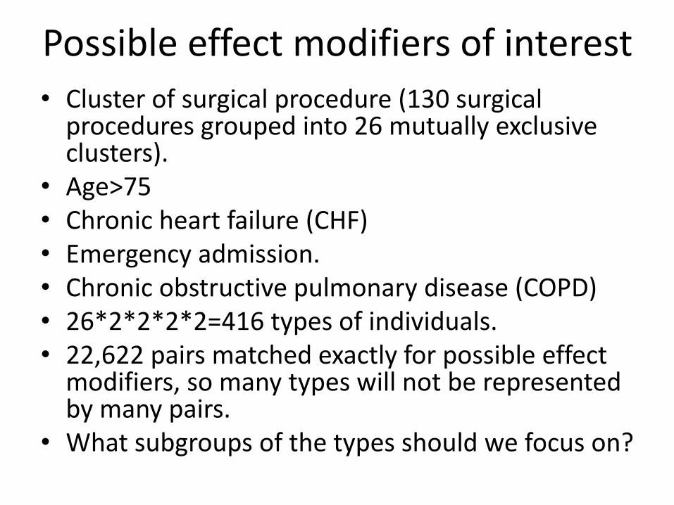
Possible effect modifiers of interest

• Cluster of surgical procedure (130 surgical procedures grouped into 26 mutually exclusive clusters).

• Age>75• Chronic heart failure (CHF)• Emergency admission.• Chronic obstructive pulmonary disease (COPD)• 26*2*2*2*2=416 types of individuals.• 22,622 pairs matched exactly for possible effect

modifiers, so many types will not be represented by many pairs.

• What subgroups of the types should we focus on?

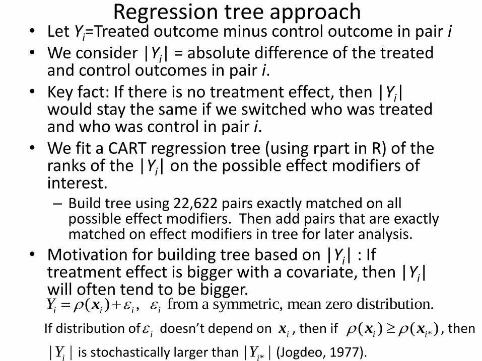
Regression tree approach• Let Yi=Treated outcome minus control outcome in pair i• We consider |Yi| = absolute difference of the treated

and control outcomes in pair i.• Key fact: If there is no treatment effect, then |Yi|

would stay the same if we switched who was treated and who was control in pair i.

• We fit a CART regression tree (using rpart in R) of the ranks of the |Yi| on the possible effect modifiers of interest.– Build tree using 22,622 pairs exactly matched on all

possible effect modifiers. Then add pairs that are exactly matched on effect modifiers in tree for later analysis.

• Motivation for building tree based on |Yi| : If treatment effect is bigger with a covariate, then |Yi| will often tend to be bigger.

( ) , from a symmetric, mean zero distribution.i i i iY x

If distribution of i doesn’t depend on ix , then if *( ) ( )i i x x , then

| |iY is stochastically larger than *| |iY (Jogdeo, 1977).

Figure 1: Mortality in 23,715 matched pairs of two Medicare patients, one receiving surgery at a magnet hospital identified for superior nursing, the other undergoing the same surgical procedure at a conventional control hospital. The three values (A,B,C) at the nodes of the tree are: A = McNemar odds ratio for mortality, control/magnet, B = 30-day mortality rate (%) at the magnet hospitals, C = 30-day mortality rate (%) at the control hospitals.

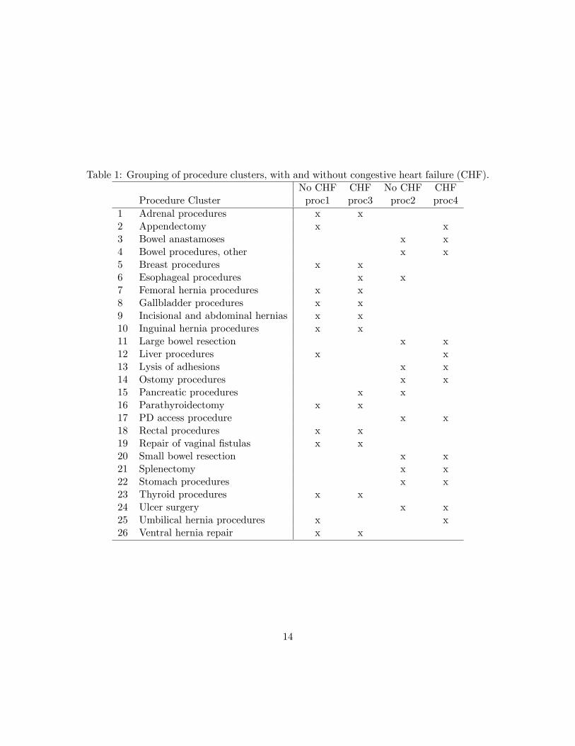
Table 1: Grouping of procedure clusters, with and without congestive heart failure (CHF).No CHF CHF No CHF CHF

Procedure Cluster proc1 proc3 proc2 proc41 Adrenal procedures x x2 Appendectomy x x3 Bowel anastamoses x x4 Bowel procedures, other x x5 Breast procedures x x6 Esophageal procedures x x7 Femoral hernia procedures x x8 Gallbladder procedures x x9 Incisional and abdominal hernias x x10 Inguinal hernia procedures x x11 Large bowel resection x x12 Liver procedures x x13 Lysis of adhesions x x14 Ostomy procedures x x15 Pancreatic procedures x x16 Parathyroidectomy x x17 PD access procedure x x18 Rectal procedures x x19 Repair of vaginal fistulas x x20 Small bowel resection x x21 Splenectomy x x22 Stomach procedures x x23 Thyroid procedures x x24 Ulcer surgery x x25 Umbilical hernia procedures x x26 Ventral hernia repair x x

14

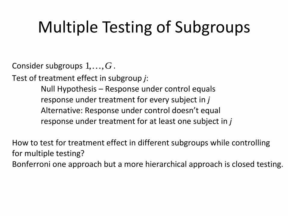
Multiple Testing of Subgroups

Consider subgroups 1, ,G .

Test of treatment effect in subgroup j: Null Hypothesis – Response under control equals response under treatment for every subject in j Alternative: Response under control doesn’t equal response under treatment for at least one subject in j

How to test for treatment effect in different subgroups while controlling for multiple testing? Bonferroni one approach but a more hierarchical approach is closed testing.

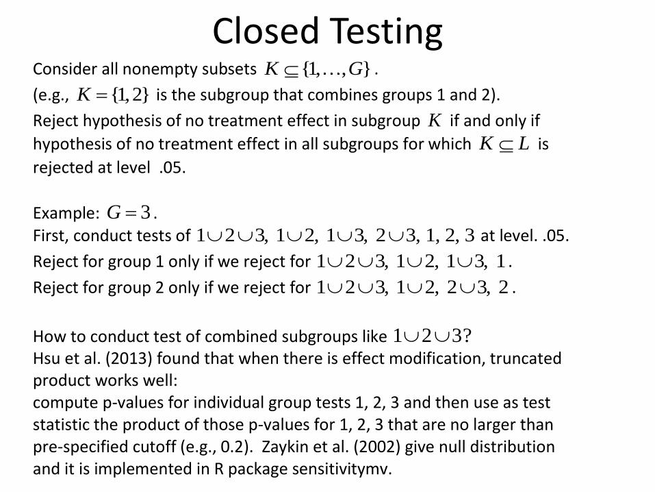
Closed TestingConsider all nonempty subsets {1, , }K G .

(e.g., {1,2}K is the subgroup that combines groups 1 and 2).

Reject hypothesis of no treatment effect in subgroup K if and only if

hypothesis of no treatment effect in all subgroups for which K L is

rejected at level .05.

Example: 3G . First, conduct tests of 1 2 3, 1 2, 1 3, 2 3, 1, 2, 3 at level. .05.

Reject for group 1 only if we reject for 1 2 3, 1 2, 1 3, 1 .

Reject for group 2 only if we reject for 1 2 3, 1 2, 2 3, 2 .

How to conduct test of combined subgroups like 1 2 3? Hsu et al. (2013) found that when there is effect modification, truncated product works well: compute p-values for individual group tests 1, 2, 3 and then use as test statistic the product of those p-values for 1, 2, 3 that are no larger than pre-specified cutoff (e.g., 0.2). Zaykin et al. (2002) give null distribution and it is implemented in R package sensitivitymv.

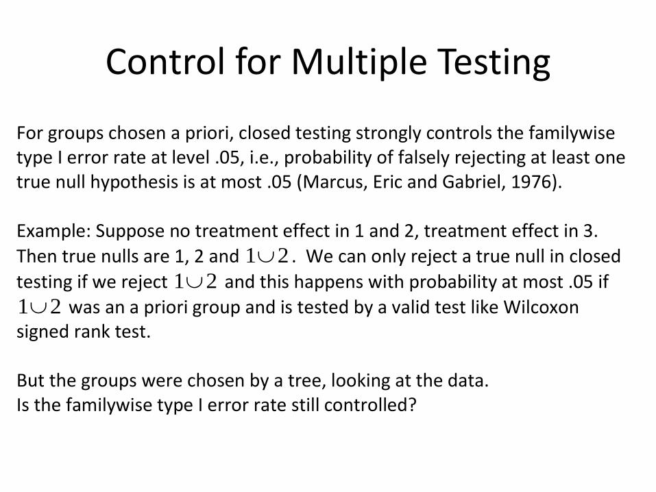
Control for Multiple Testing

For groups chosen a priori, closed testing strongly controls the familywise type I error rate at level .05, i.e., probability of falsely rejecting at least one true null hypothesis is at most .05 (Marcus, Eric and Gabriel, 1976). Example: Suppose no treatment effect in 1 and 2, treatment effect in 3.

Then true nulls are 1, 2 and 1 2 . We can only reject a true null in closed

testing if we reject 1 2 and this happens with probability at most .05 if

1 2 was an a priori group and is tested by a valid test like Wilcoxon signed rank test. But the groups were chosen by a tree, looking at the data. Is the familywise type I error rate still controlled?

Control for Multiple Testing ContinuedSimple case: Suppose there’s no overall treatment effect (i.e., null for

1 2 3 true).

We formed tree by regressing | |iY on ix .

Consider a pair in which there’s no treatment effect,

Subject 1 Subject 2

Control Response

Treatment Response

Control Response

Treatment Response

Pair 1 3 3 2 2

If subject 1 is assigned treatment and subject 2 control, 1iY .

If subject 1 is assigned control and subject 2 treatment, 1iY .

Thus, | |iY always equals 1.

If there’s no overall treatment effect and we consider the randomization distribution of a test statistic when one subject in each pair randomly

assigned to treatment, then the | |iY ’s will always be the same and the

tree will always be the same. Thus, groups are in some sense chosen a priori when no overall treatment effect and familywise Type I error rate is controlled.

More complicated case: Treatment effect in some pairs but not others.

Subject 1 Subject 2

Control Response

Treatment Response

Control Response

Treatment Response

Pair 1 2 2 3 3

Pair 2 4 4 6 6

Pair 3 2 3 4 7

Consider the subgroup of pairs 1 and 2 in which there’s no treatment effect. The tree will not depend on which subject gets assigned to treatment in

pairs 1 and 2 since the | |iY is fixed but may depend on the assignment

in pair 3, since | | 1iY if subject 1 assigned to treatment, | | 5iY if subject 2

assigned to treatment. Suppose that the tree only creates pairs 1 and 2 as a subgroup if subject 1 in pair 3 is assigned to treatment. Assuming random assignment in each pair, when pairs 1 and 2 are created as a subgroup, the assignment of treatment in pairs 1 and 2 is random. Thus, when a hypothesis for the subgroup of pairs 1 and 2 is tested, the distribution of treatment assignments in pairs 1 and 2 is random and can be validly tested with Wilcoxon signed rank test or other permutation tests.

Strong Control of Familywise Error Rate

Proposition: The closed testing procedure with the tree

formed by regressing | |iY on ix has probability at most

.05 of falsely rejecting a true null hypothesis.

Table 2: Mortality in 23,715 matched pairs of a patient receiving surgery at a magnethospital or a control hospital, where the pairs have been divided into five groups selectedby CART. A sensitivity analysis using McNemar’s test examines mortality in each group,combining group specific results using the truncated product of P -values, truncated at 0.1.The control/magnet odds ratio associated with McNemar’s test is given.

Subgroups PooledGroup 1 Group 2 Group 3 Group 4 Group5

CHF no no no yes yesProcedures proc1 proc2 proc2 proc3 proc4ER admission both no yes both bothNumber of Pairs 10127 5636 2943 2086 2923 23715Discordant Pairs 210 293 488 217 760 1968

Percent Discordant % 2.1 5.2 16.6 10.4 26.0 8.3Odds Ratio 1.41 1.53 1.09 1.28 1.18 1.23

Morality %, Magnet 0.9 2.5 10.1 4.9 16.5 4.7Morality %, Control 1.3 3.5 10.8 6.2 18.6 5.6

Sensitivity analysis: Upper bounds on P -values for various Γ

Γ Subgroups TruncatedGroup 1 Group 2 Group 3 Group 4 Group 5 Product

1.00 0.008 0.000 0.195 0.039 0.013 0.0001.05 0.019 0.001 0.374 0.080 0.062 0.0001.10 0.042 0.003 0.576 0.143 0.184 0.0121.15 0.079 0.010 0.753 0.230 0.386 0.0321.17 0.099 0.015 0.809 0.270 0.479 0.0441.20 0.135 0.025 0.875 0.335 0.616 0.163

15

Sensitivity analysis• Analysis so far has assumed random

assignment of treatment in a matched pair.• But nursing study is an observational study.• Central concern in observational study:

assignment of treatment nonrandom, related to unmeasured confounders.

• Sensitivity analysis: How sensitive are conclusions to allowing for some amount of unmeasured confounding?

• Original sensitivity analysis: – Fisher asserted that smoking had no causal

effect on lung cancer, association due to unmeasured genetic variant.

– Cornfield et al. (1959) showed that genetic variant would have to be 9 times more likely among smokers than nonsmokers for association to be non-causal.

Model for sensitivity analysisConsider matched pair – the subjects in the matched pair have (approximately) the same observed covariates x . Suppose there’s an unmeasured confounder u that might differ between subjects in a matched pair. Let be the maximum ratio of odds of subject 1 getting treated compared to subject 2 because of differences in u .

1 : Effectively random assignment, u doesn’t affect treatment assignment

2 : Unit with higher u could have double the odds of treatment.

3 : Unit with higher u could have triple the odds of treatment. For a given , we can test the null hypothesis of no treatment effect (Rosenbaum, 2002, Observational Studies, Ch. 4). Our proposition extends to sensitivity analysis to say that forming the tree by

regressing | |iY on ix and then applying the closed testing procedure with

sensitivity analysis tests that allow for unmeasured confounding up to has probability at most .05 of falsely rejecting a true null assuming the unmeasured confounding is at most .

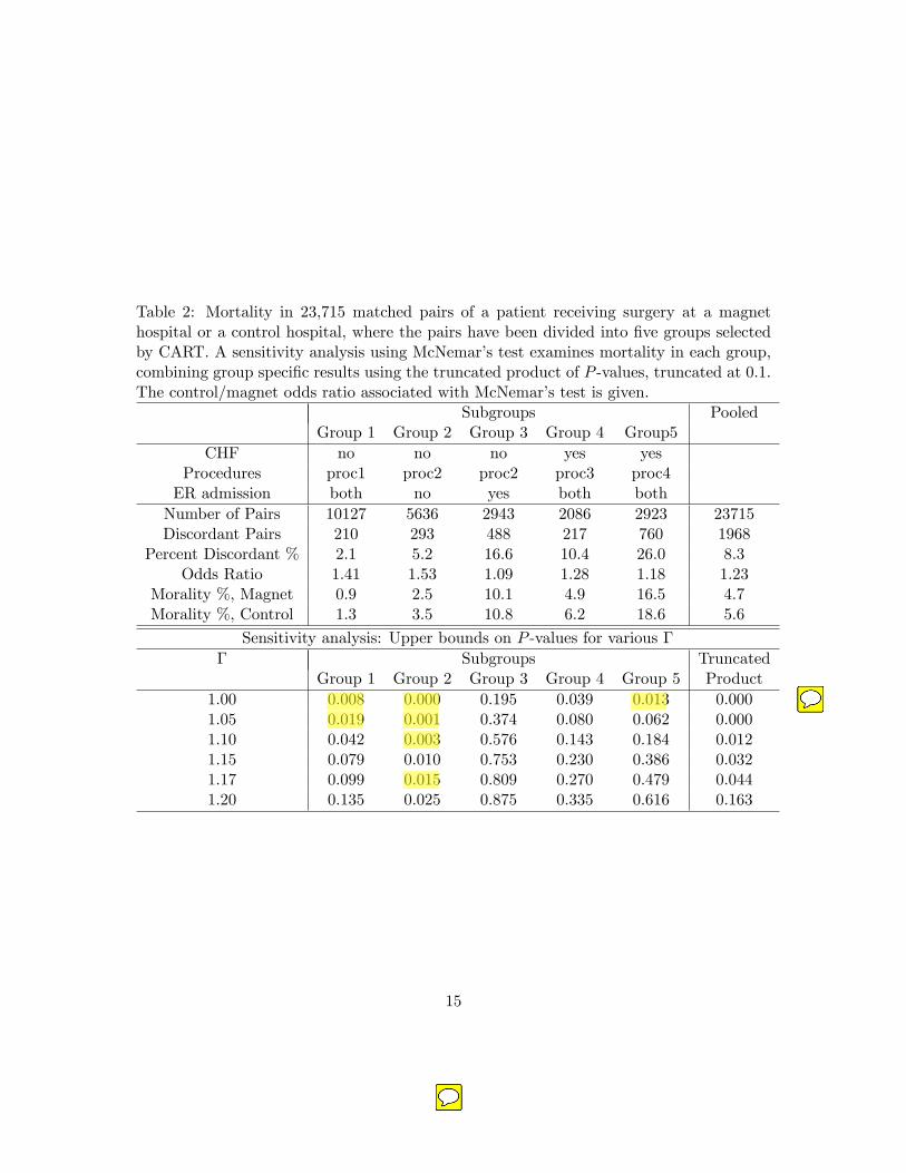
Table 2: Mortality in 23,715 matched pairs of a patient receiving surgery at a magnethospital or a control hospital, where the pairs have been divided into five groups selectedby CART. A sensitivity analysis using McNemar’s test examines mortality in each group,combining group specific results using the truncated product of P -values, truncated at 0.1.The control/magnet odds ratio associated with McNemar’s test is given.

Subgroups PooledGroup 1 Group 2 Group 3 Group 4 Group5

CHF no no no yes yesProcedures proc1 proc2 proc2 proc3 proc4ER admission both no yes both bothNumber of Pairs 10127 5636 2943 2086 2923 23715Discordant Pairs 210 293 488 217 760 1968

Percent Discordant % 2.1 5.2 16.6 10.4 26.0 8.3Odds Ratio 1.41 1.53 1.09 1.28 1.18 1.23

Morality %, Magnet 0.9 2.5 10.1 4.9 16.5 4.7Morality %, Control 1.3 3.5 10.8 6.2 18.6 5.6

Sensitivity analysis: Upper bounds on P -values for various Γ

Γ Subgroups TruncatedGroup 1 Group 2 Group 3 Group 4 Group 5 Product

1.00 0.008 0.000 0.195 0.039 0.013 0.0001.05 0.019 0.001 0.374 0.080 0.062 0.0001.10 0.042 0.003 0.576 0.143 0.184 0.0121.15 0.079 0.010 0.753 0.230 0.386 0.0321.17 0.099 0.015 0.809 0.270 0.479 0.0441.20 0.135 0.025 0.875 0.335 0.616 0.163

15

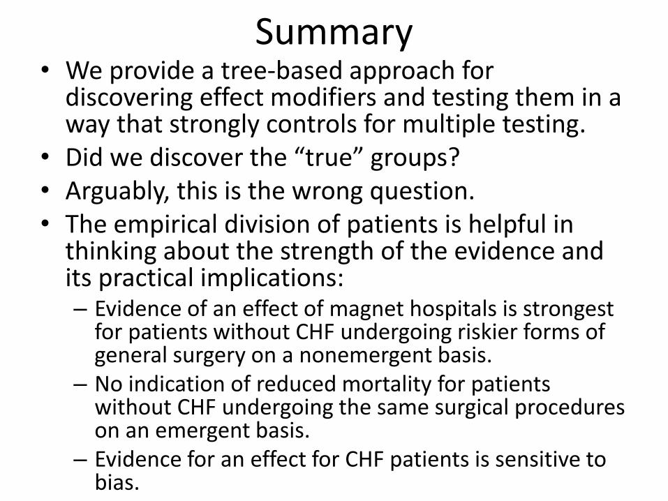
Summary• We provide a tree-based approach for

discovering effect modifiers and testing them in a way that strongly controls for multiple testing.

• Did we discover the “true” groups? • Arguably, this is the wrong question.• The empirical division of patients is helpful in

thinking about the strength of the evidence and its practical implications:– Evidence of an effect of magnet hospitals is strongest

for patients without CHF undergoing riskier forms of general surgery on a nonemergent basis.

– No indication of reduced mortality for patients without CHF undergoing the same surgical procedures on an emergent basis.

– Evidence for an effect for CHF patients is sensitive to bias.

References• Hsu, J.Y., Small, D.S. and Rosenbaum, P.R. (2013).

Effect and modification and design sensitivity in observational studies. J. Am. Statist. Assoc., 108, 135-148.

• Hsu, J.Y., Zubizarreta, J.R., Small, D.S. and Rosenbaum, P.R. (2015). Strong control of the family-wise error rate in observational studies that discover effect modification by exploratory methods. Biometrika, in press.

• Lee, K., Small, D.S., Hsu, J.Y., Silber, J.H. and Rosenbaum, P.R. Discovering Effect Modification in an Observational Study of Surgical Mortality at Hospitals with Superior Nursing. Under Review.

• Thanks!

Simulation Study

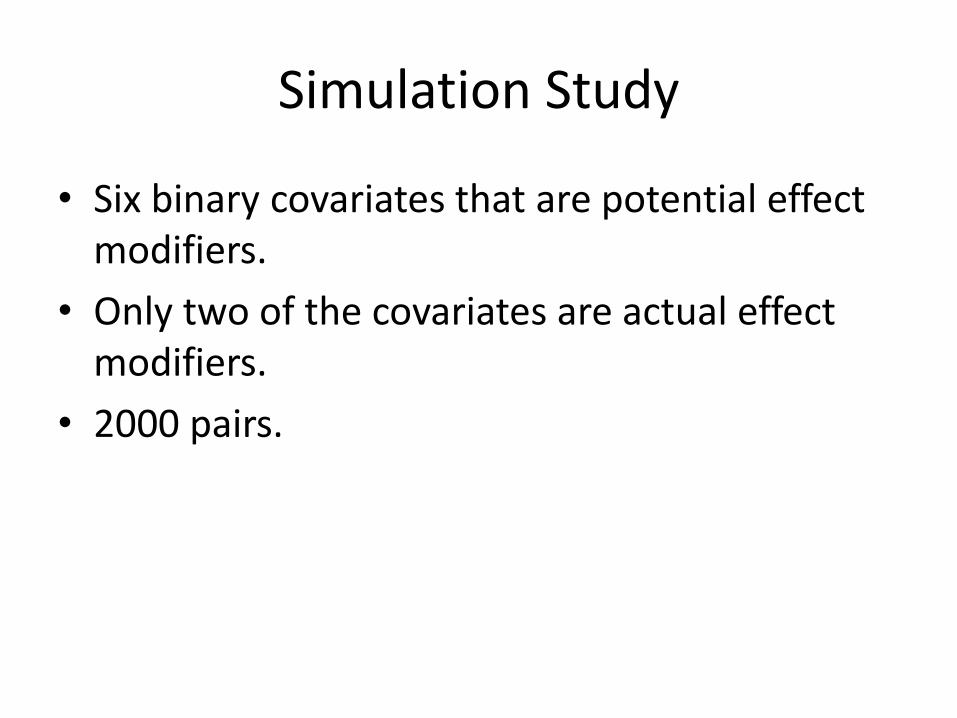
• Six binary covariates that are potential effect modifiers.

• Only two of the covariates are actual effect modifiers.

• 2000 pairs.

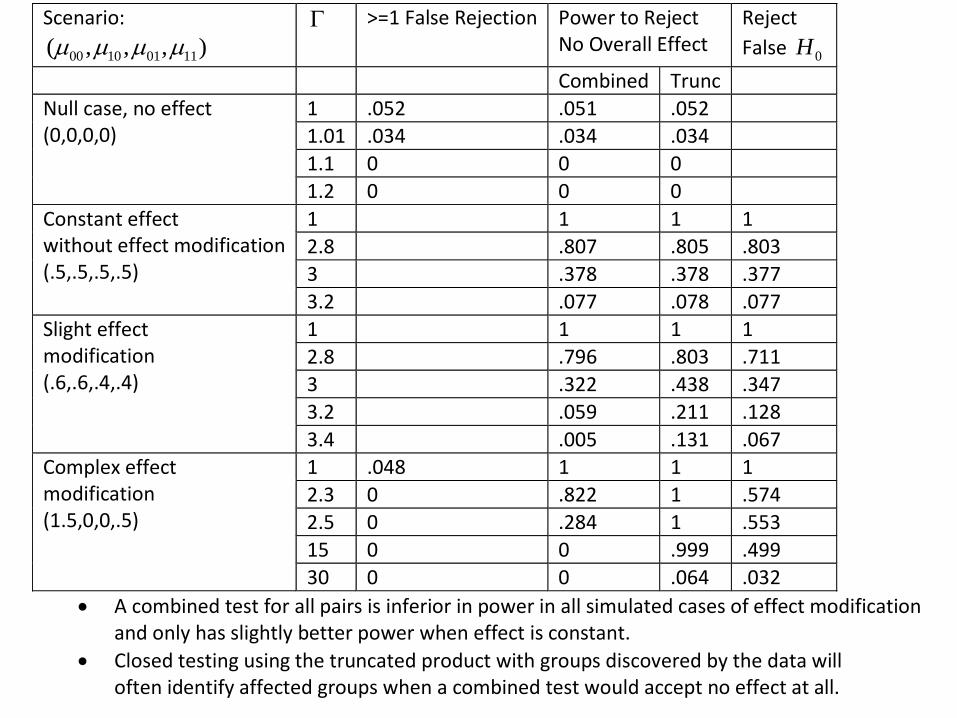
Scenario:

00 10 01 11( , , , )

>=1 False Rejection Power to Reject No Overall Effect

Reject

False 0H

Combined Trunc

Null case, no effect (0,0,0,0)

1 .052 .051 .052

1.01 .034 .034 .034

1.1 0 0 0

1.2 0 0 0

Constant effect without effect modification (.5,.5,.5,.5)

1 1 1 1

2.8 .807 .805 .803

3 .378 .378 .377

3.2 .077 .078 .077

Slight effect modification (.6,.6,.4,.4)

1 1 1 1

2.8 .796 .803 .711

3 .322 .438 .347

3.2 .059 .211 .128

3.4 .005 .131 .067

Complex effect modification (1.5,0,0,.5)

1 .048 1 1 1

2.3 0 .822 1 .574

2.5 0 .284 1 .553

15 0 0 .999 .499

30 0 0 .064 .032

A combined test for all pairs is inferior in power in all simulated cases of effect modification and only has slightly better power when effect is constant.

Closed testing using the truncated product with groups discovered by the data will often identify affected groups when a combined test would accept no effect at all.