dirty holographic superconductors - centre de recherches … · 2015-10-30 · dirty holographic...

Dirty Holographic Superconductors

Leopoldo Pando ZayasICTP, Trieste/University of Michigan

Applications of AdS/CFT to QCD and Condensed Matter PhysicsOctober 20, CRM, Montreal, Canada

Based on 1308.1920 (PRD), 1407.7526 (JHEP), 1507.02280Work in Progress, D. Arean, LPZ, I. Salazar, A. Scardicchio

Leopoldo Pando Zayas (ICTP/Michigan) Dirty Superconductors Talk 1 / 43

Outline

Outline

Motivation: Anderson localization, Many Body Localization, DirtySuperconductors.

A numerical approach to disorder in AdS/CFT.

Disordered Holographic s- and p-wave Superconductor.

Enhancement of superconductivity for mild disorder and a universalityin the responses.

Conductivity: Superconductor-Metal Transition.

Outlook


Motivation

Motivation: Big Picture

What is the AdS/CFT correspondence an answer to?

QCD?

Phase transitions and infinite correlation length: ξ ∼ |p− pc|−ν(CFT).

K. Wilson already answered this question with RG. Critical exponentsare universal, independent of the microscopic details (WF). Permissionto approach the fixed points any way you can, including AdS/CFT.

Critical exponents for strongly coupled systems.

Critical exponents for disorder-driven strongly coupled transitions.

Dynamical critical exponents in time-dependent systems (quenches,thermalization ...).


Motivation

Motivation: Transport and Disorder

Most systems are not clean!

Problem (AdS/CM): Transport and translational symmetry/absenceof momentum dissipation.

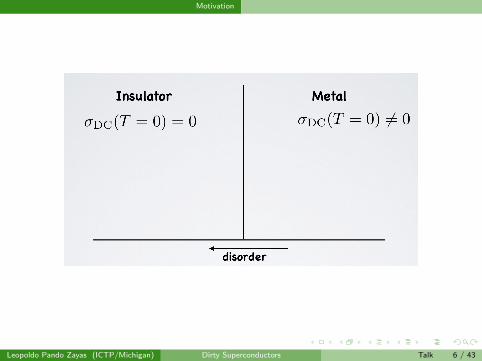
Anderson Localization: The conductivity can be completelysuppressed by quantum effects.

Many Body Localization for isolated quantum systems: Andersonlocalization persists in the presence of finite interactions.


Motivation

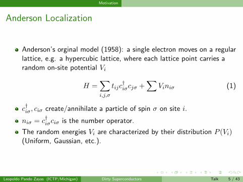
Anderson Localization

Anderson’s orginal model (1958): a single electron moves on a regularlattice, e.g. a hypercubic lattice, where each lattice point carries arandom on-site potential Vi

H =∑i,j,σ

tijc†iσcjσ +

∑Viniσ (1)

c†iσ, ciσ create/annihilate a particle of spin σ on site i.

niσ = c†iσciσ is the number operator.

The random energies Vi are characterized by their distribution P (Vi)(Uniform, Gaussian, etc.).


Motivation


Motivation

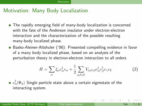
Motivation: Many Body Localization

The rapidly emerging field of many-body localization is concernedwith the fate of the Anderson insulator under electron-electroninteraction and the characterization of the possible resultingmany-body localized phase.

Basko-Aleiner-Altshuler (’06): Presented compelling evidence in favorof a many body localized phase, based on an analysis of theperturbation theory in electron-electron interaction to all orders

H =∑α

ξαc†αcα +

1

2

∑αβγδ

Vαβγδc†αc†βcγcδ (2)

c†α|Ψk〉 Single particle state above a certain eigenstate of theinteracting system.


Motivation

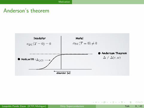
Anderson’s Theorem

Anderson’s Theorem (Journal of Physics and Chemistry, 58):Superconductivity is insensitive to perturbations that do not destroytime-reversal invariance (pair breaking). This provided the centralintuition.

Critiques to Anderson’s argument were raised, for example, byconsidering the effects of strong localization: A. Kapitulnik, G.

Kotliar, Phys. Rev. Lett. 54, 473, (1985). G.

Kotliar, A. Kapitulnik, Phys. Rev. B 33, 3146 (1986),

M. Ma, P.A. Lee, Phys. Rev. B 32, 5658, (1985).

More generally, the question of the role of interactions, in particular,the Coulomb interaction in dirty superconductors cannot beconsidered settled.


Motivation

Anderson’s theorem


Motivation

What is AdS/CFT doing about momentum dissipation?

Massive gravity:

I Vegh: Holography without translational symmetryI Tong, Andrade,Davidson, ....

Disorder (After our work):

I Hartnoll and Santos: Disordered horizons: Holography of randomlydisordered fixed points

I Lucas, Sachdev and Schalm: Scale-invariant hyperscaling-violatingholographic theories and the resistivity of strange metals withrandom-field disorder

I O’Keeffe and Peet: Perturbatively charged holographic disorder


Disordered holographic s-wave superconductor


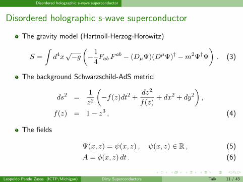
The gravity model (Hartnoll-Herzog-Horowitz)

S =

∫d4x√−g(−1

4Fab F

ab − (DµΨ)(DµΨ)† −m2Ψ†Ψ

). (3)

The background Schwarzschild-AdS metric:

ds2 =1

z2

(−f(z)dt2 +

dz2

f(z)+ dx2 + dy2

),

f(z) = 1− z3 , (4)

The fields

Ψ(x, z) = ψ(x, z) , ψ(x, z) ∈ R , (5)

A = φ(x, z) dt . (6)



Boundary Conditions: Spontaneously broken symmetry

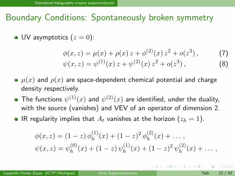
UV asymptotics (z = 0):

φ(x, z) = µ(x) + ρ(x) z + φ(2)(x) z2 + o(z3) , (7)

ψ(x, z) = ψ(1)(x) z + ψ(2)(x) z2 + o(z3) , (8)

µ(x) and ρ(x) are space-dependent chemical potential and chargedensity respectively.

The functions ψ(1)(x) and ψ(2)(x) are identified, under the duality,with the source (vanishes) and VEV of an operator of dimension 2.

IR regularity implies that At vanishes at the horizon (zh = 1).

φ(x, z) = (1− z)φ(1)h (x) + (1− z)2 φ

(2)h (x) + . . . ,

ψ(x, z) = ψ(0)h (x) + (1− z)ψ(1)

h (x) + (1− z)2 ψ(2)h (x) + . . . ,



Introducing disorder in the holographic s-wavesuperconductor

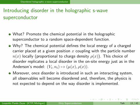
What? Promote the chemical potential in the holographicsuperconductor to a random space-dependent function.

Why? The chemical potential defines the local energy of a chargedcarrier placed at a given position x coupling with the particle numbern(x) locally (proportional to charge density ρ(x)). This choice ofdisorder replicates a local disorder in the on-site energy just as in theAnderson’s model: (Vi, ni) 7→ (µ(x), ρ(x)).

Moreover, once disorder is introduced in such an interacting system,all observables will become disordered and, therefore, the physics isnot expected to depend on the way disorder is implemented.



Disorder in details

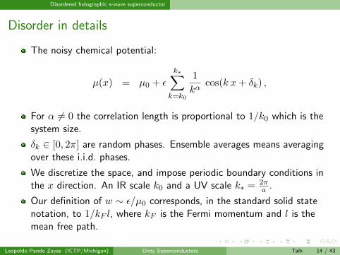
The noisy chemical potential:

µ(x) = µ0 + ε

k∗∑k=k0

1

kαcos(k x+ δk) ,

For α 6= 0 the correlation length is proportional to 1/k0 which is thesystem size.

δk ∈ [0, 2π] are random phases. Ensemble averages means averagingover these i.i.d. phases.

We discretize the space, and impose periodic boundary conditions inthe x direction. An IR scale k0 and a UV scale k∗ = 2π

a .

Our definition of w ∼ ε/µ0 corresponds, in the standard solid statenotation, to 1/kF l, where kF is the Fermi momentum and l is themean free path.



Numerics

Most of the simulations were done independently in Mathematica andin Python. The latter ones ran in the University of Michigan Fluxcluster.

Our typical result contains a grid of 100× 100 points but we havegone up to 200× 200 to control issues of convergence andoptimization.

We used a relaxation algorithm to search for the solution and use anL2 measure for convergence which in most cases reached 10−16. Asthe source of randomness we used µ(x) (sum of cosines) and also foruniform and Gaussian distributions.



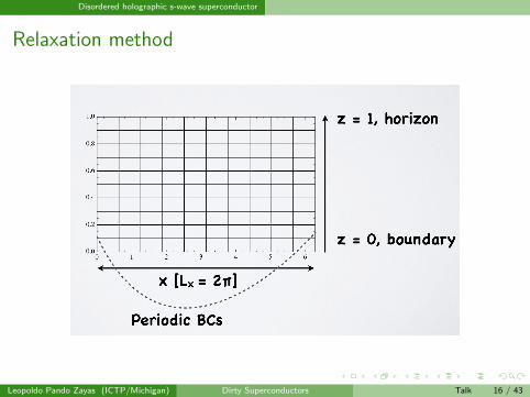
Relaxation method



Condensate versus noise strength

The value of the condensate grows with increasing disorder strength,w



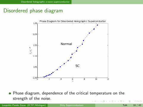
Disordered phase diagram

Phase diagram, dependence of the critical temperature on thestrength of the noise.



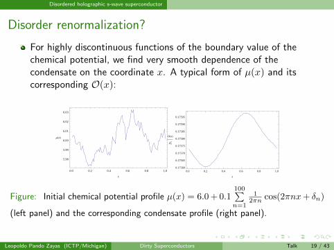
Disorder renormalization?

For highly discontinuous functions of the boundary value of thechemical potential, we find very smooth dependence of thecondensate on the coordinate x. A typical form of µ(x) and itscorresponding O(x):

0.0 0.2 0.4 0.6 0.8 1.0

5.98

5.99

6.00

6.01

6.02

6.03

x

ΜHxL

0.0 0.2 0.4 0.6 0.8 1.00.17560

0.17565

0.17570

0.17575

0.17580

0.17585

0.17590

0.17595

x

OHxL

Μ02

Figure: Initial chemical potential profile µ(x) = 6.0 + 0.1100∑n=1

12πn cos(2πnx+ δn)

(left panel) and the corresponding condensate profile (right panel).



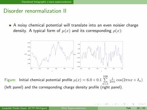
Disorder renormalization II

A noisy chemical potential will translate into an even noisier chargedensity. A typical form of µ(x) and its corresponding ρ(x):

0.0 0.2 0.4 0.6 0.8 1.0

5.98

5.99

6.00

6.01

6.02

6.03

x

ΜHxL

0.0 0.2 0.4 0.6 0.8 1.0

-10.6

-10.4

-10.2

-10.0

-9.8

-9.6

x

ΡHxL

Figure: Initial chemical potential profile µ(x) = 6.0 + 0.1100∑n=1

12πn cos(2πnx+ δn)

(left panel) and the corresponding charge density profile (right panel).



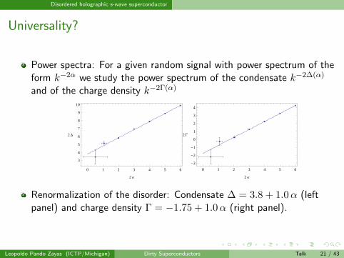
Universality?

Power spectra: For a given random signal with power spectrum of theform k−2α we study the power spectrum of the condensate k−2∆(α)

and of the charge density k−2Γ(α)

0 1 2 3 4 5 6

3

4

5

6

7

8

9

10

2 Α

2 D

0 1 2 3 4 5 6

-3

-2

-1

0

1

2

3

4

2 Α

2 G

Renormalization of the disorder: Condensate ∆ = 3.8 + 1.0α (leftpanel) and charge density Γ = −1.75 + 1.0α (right panel).


Disorder Holographic P-wave Super Conductor

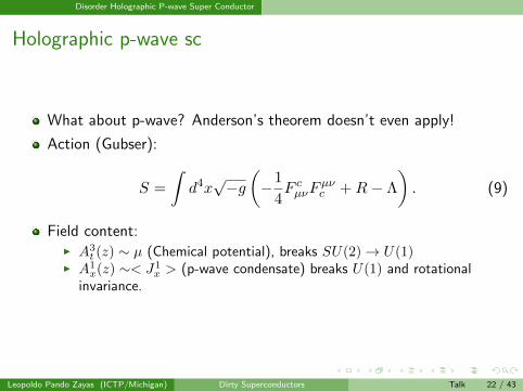
Holographic p-wave sc

What about p-wave? Anderson’s theorem doesn’t even apply!

Action (Gubser):

S =

∫d4x√−g(−1

4F cµνF

µνc +R− Λ

). (9)

Field content:I A3

t (z) ∼ µ (Chemical potential), breaks SU(2)→ U(1)I A1

x(z) ∼< J1x > (p-wave condensate) breaks U(1) and rotational

invariance.



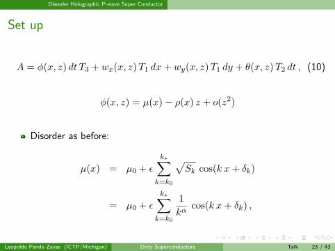
Set up

A = φ(x, z) dt T3 + wx(x, z)T1 dx+ wy(x, z)T1 dy + θ(x, z)T2 dt , (10)

φ(x, z) = µ(x)− ρ(x) z + o(z2)

Disorder as before:

µ(x) = µ0 + ε

k∗∑k=k0

√Sk cos(k x+ δk)

= µ0 + ε

k∗∑k=k0

1

kαcos(k x+ δk) ,



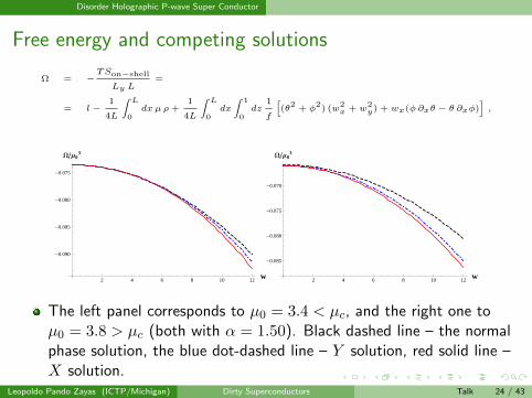
Free energy and competing solutions

Ω = −TSon−shell

Ly L=

= l−1

4L

∫ L

0dxµ ρ +

1

4L

∫ L

0dx

∫ 1

0dz

1

f

[(θ

2+ φ

2) (w

2x + w

2y) + wx(φ ∂xθ − θ ∂xφ)

],

2 4 6 8 10 12w

-0.090

-0.085

-0.080

-0.075

WΜ03

2 4 6 8 10 12w

-0.085

-0.080

-0.075

-0.070

WΜ03

The left panel corresponds to µ0 = 3.4 < µc, and the right one toµ0 = 3.8 > µc (both with α = 1.50). Black dashed line – the normalphase solution, the blue dot-dashed line – Y solution, red solid line –X solution.



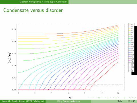
Condensate versus disorder

0 2 4 6 8 10 12

0.00

0.05

0.10

0.15

0.20

0.25

w

Xwx

\Μ0

2

CT3.3.053.13.153.23.253.33.353.43.453.53.553.63.653.73.83.94.4.14.24.34.44.5

Figure: Spatial average of the condensate as a function of the strength ofdisorder. Each line corresponds to an average over 10 realizations of noise (withα = 1.50) on a lattice of size 22× 40. The value of the condensate grows withincreasing disorder strength, w. Each line corresponds to a value of µ0 asindicated on the legend, but for the black dashed line which, as explained in thetext, marks the cut off used to define the critical temperature.



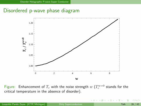
Disordered p-wave phase diagram

0 2 4 6 8

1.00

1.05

1.10

1.15

1.20

w

Tc

T

cw=

0

Figure: Enhancement of Tc with the noise strength w (Tw=0c stands for the

critical temperature in the absence of disorder).


The Holographic Disorder-Driven Superconductor-MetalTransition

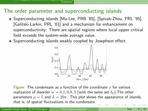
The order parameter and superconducting islandsSuperconducting islands [Ma-Lee, PRB ’85], [Spivak-Zhou, PRL ’95],[Galitski-Larkin, PRL ’01] and a mechanism for enhancement onsuperconductivity: There are spatial regions where local upper criticalfield exceeds the system-wide average value.Superconducting islands weakly coupled by Josephson effect.

0 20 40 60 800.0

0.2

0.4

0.6

0.8

90×x H20ΠL

O2

Μ2

Figure: The condensate as a function of the coordinate x for variousrealization of disorder w = 0.1, 0.9, 3 (with the same set δk).The otherparameters µ = 5 and L = 20π. This plot shows the appearance of islands,that is, of spatial fluctuations in the condensate.



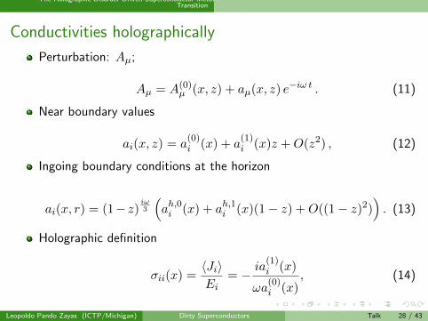
Conductivities holographically

Perturbation: Aµ;

Aµ = A(0)µ (x, z) + aµ(x, z) e−iω t . (11)

Near boundary values

ai(x, z) = a(0)i (x) + a

(1)i (x)z +O(z2) , (12)

Ingoing boundary conditions at the horizon

ai(x, r) = (1− z)iω3

(ah,0i (x) + ah,1i (x)(1− z) +O((1− z)2)

). (13)

Holographic definition

σii(x) =〈Ji〉Ei

= −ia

(1)i (x)

ωa(0)i (x)

, (14)



Conductivities holographically: Superfluid Density

Conductivities at low frequencies and Kramers-Kronig

σ ≈ ns(πδ(ω) +

i

ω

). (15)

The superfluid density ns



0.0 0.5 1.0 1.5 2.0 2.5 3.0 3.50.0

0.2

0.4

0.6

0.8

1.0

w

ns

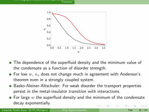
The dependence of the superfluid density and the minimum value ofthe condensate as a function of disorder strength.

For low w, ns does not change much in agreement with Anderson’stheorem even in a strongly coupled system.

Basko-Aleiner-Altschuler: For weak disorder the transport propertiespersist in the metal-insulator transition with interactions.

For large w the superfluid density and the minimum of the condensatedecay exponentially.



Conductivities holographically

The Plot <(σ)

New resonances

spectral shift

0 2 4 6 80.0

0.2

0.4

0.6

0.8

1.0

Ω

Re

HΣL

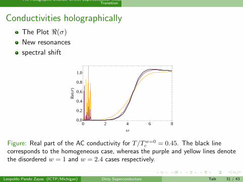
Figure: Real part of the AC conductivity for T/Tw=0c = 0.45. The black line

corresponds to the homogeneous case, whereas the purple and yellow lines denotethe disordered w = 1 and w = 2.4 cases respectively.



0 2 4 6 80.0

0.2

0.4

0.6

0.8

1.0

Ω

Re

HΣL

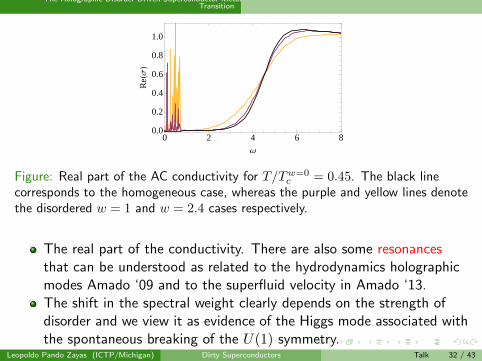
Figure: Real part of the AC conductivity for T/Tw=0c = 0.45. The black line

corresponds to the homogeneous case, whereas the purple and yellow lines denotethe disordered w = 1 and w = 2.4 cases respectively.

The real part of the conductivity. There are also some resonancesthat can be understood as related to the hydrodynamics holographicmodes Amado ‘09 and to the superfluid velocity in Amado ‘13.The shift in the spectral weight clearly depends on the strength ofdisorder and we view it as evidence of the Higgs mode associated withthe spontaneous breaking of the U(1) symmetry.



0.5 0.6 0.7 0.8 0.9 1.0

T

T c

0.1

0.2

0.3

0.4

0.5

0.6

0.7

v s

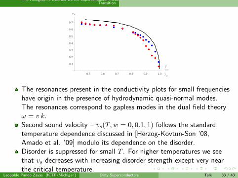
The resonances present in the conductivity plots for small frequencieshave origin in the presence of hydrodynamic quasi-normal modes.The resonances correspond to gapless modes in the dual field theoryω = v k.Second sound velocity – vs(T,w = 0, 0.1, 1) follows the standardtemperature dependence discussed in [Herzog-Kovtun-Son ’08,Amado et al. ’09] modulo its dependence on the disorder.Disorder is suppressed for small T . For higher temperatures we seethat vs decreases with increasing disorder strength except very nearthe critical temperature.



Phase Transitions and Mean Field Theory

Landau theory and critical exponents:

F = a+ bΨ2 + cΨ4 + . . . (16)

At the critical temperature, Tc, the minimum goes from Ψ = 0 toΨ = when b changes sign.

Ψ = ±√−b0(T − Tc)

a(17)

Critical exponent β = 1/2, generally Ψ ∼ |T − Tc|β.

Wilson: β from RG, that is, scaling.

What about disordered phase transitions?



Field theory approach to disordered fixed points

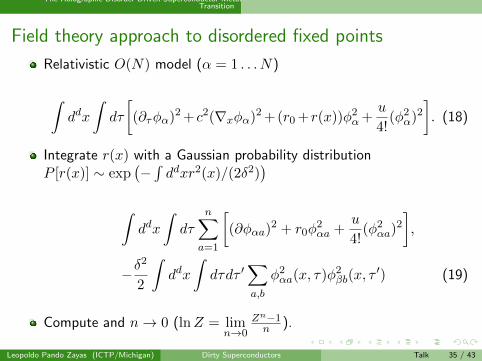
Relativistic O(N) model (α = 1 . . . N)

∫ddx

∫dτ

[(∂τφα)2 + c2(∇xφα)2 +(r0 +r(x))φ2

α+u

4!(φ2α)2

]. (18)

Integrate r(x) with a Gaussian probability distributionP [r(x)] ∼ exp

(−∫ddxr2(x)/(2δ2)

)∫ddx

∫dτ

n∑a=1

[(∂φαa)

2 + r0φ2αa +

u

4!(φ2αa)

2

],

−δ2

2

∫ddx

∫dτdτ ′

∑a,b

φ2αa(x, τ)φ2

βb(x, τ′) (19)

Compute and n→ 0 (lnZ = limn→0

Zn−1n ).



The disordered fixed point: Status

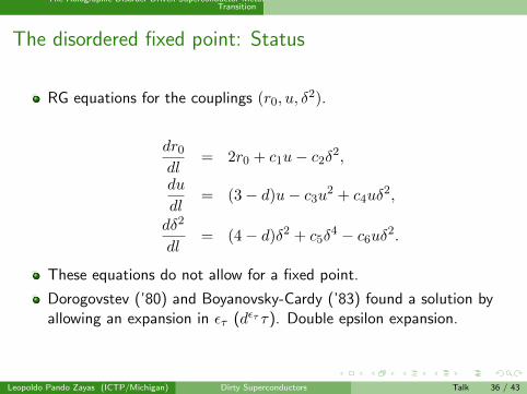
RG equations for the couplings (r0, u, δ2).

dr0

dl= 2r0 + c1u− c2δ

2,

du

dl= (3− d)u− c3u

2 + c4uδ2,

dδ2

dl= (4− d)δ2 + c5δ

4 − c6uδ2.

These equations do not allow for a fixed point.

Dorogovstev (’80) and Boyanovsky-Cardy (’83) found a solution byallowing an expansion in ετ (dετ τ). Double epsilon expansion.



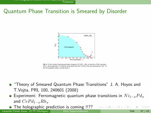
Quantum Phase Transition is Smeared by Disorder

“Theory of Smeared Quantum Phase Transitions” J. A. Hoyos andT.Vojta, PRL 100, 240601 (2008)Experiment: Ferromagnetic quantum phase transitions in Ni1−xPdxand CePd1−xRhxThe holographic prediction is coming !!??



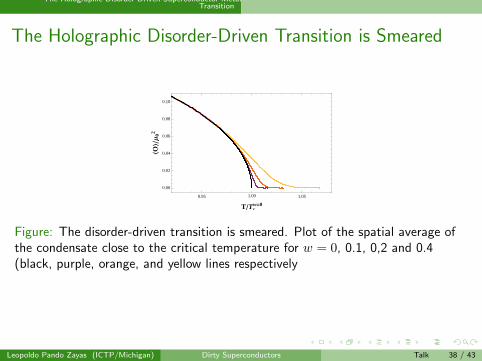
The Holographic Disorder-Driven Transition is Smeared

0.95 1.00 1.05

0.00

0.02

0.04

0.06

0.08

0.10

TTcw=0

XO\

Μ02

Figure: The disorder-driven transition is smeared. Plot of the spatial average ofthe condensate close to the critical temperature for w = 0, 0.1, 0,2 and 0.4(black, purple, orange, and yellow lines respectively



The Holographic Disorder-Driven Transition is Smeared:BKT

-6 -5 -4 -3

2

3

4

5

6

7

LogHTc-TL

Log

HXO\'

XO\L

Figure: We plot log(

1O

dOdT

)versus log(Tc − T ) for w = 0.1, 0.2, 0.4 (purple,

orange, and yellow respectively).

The order parameter behaves as 〈O〉 ∼ exp (−A|T − Tc|−ν).

Tc is different for each value of w, and is always higher than Tw=0c .

ν = 1.03± 0.02 independent of the disorder w.


Thin Films

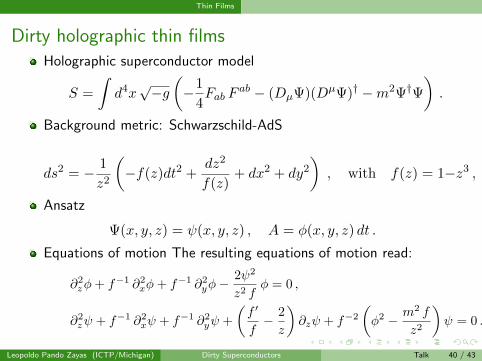
Dirty holographic thin filmsHolographic superconductor model

S =

∫d4x√−g(−1

4Fab F

ab − (DµΨ)(DµΨ)† −m2Ψ†Ψ

).

Background metric: Schwarzschild-AdS

ds2 = − 1

z2

(−f(z)dt2 +

dz2

f(z)+ dx2 + dy2

), with f(z) = 1−z3 ,

Ansatz

Ψ(x, y, z) = ψ(x, y, z) , A = φ(x, y, z) dt .

Equations of motion The resulting equations of motion read:

∂2zφ+ f−1 ∂2xφ+ f−1 ∂2yφ−2ψ2

z2 fφ = 0 ,

∂2zψ + f−1 ∂2xψ + f−1 ∂2yψ +

(f ′

f− 2

z

)∂zψ + f−2

(φ2 − m2 f

z2

)ψ = 0 .


Thin Films

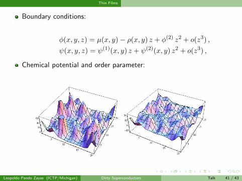
Boundary conditions:

φ(x, y, z) = µ(x, y)− ρ(x, y) z + φ(2) z2 + o(z3) ,

ψ(x, y, z) = ψ(1)(x, y) z + ψ(2)(x, y) z2 + o(z3) ,

Chemical potential and order parameter:


Thin Films

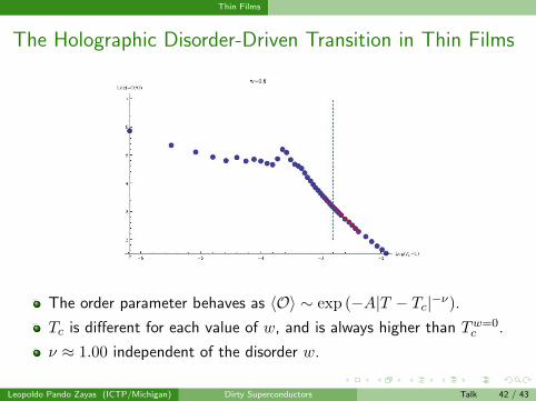
The Holographic Disorder-Driven Transition in Thin Films

The order parameter behaves as 〈O〉 ∼ exp (−A|T − Tc|−ν).

Tc is different for each value of w, and is always higher than Tw=0c .

ν ≈ 1.00 independent of the disorder w.


Outlook

Outlook

Implementation of disorder in AdS/CFT for a s- and p-waveholographic superconductor.

Better understanding of the x-dependent behavior; power spectra ofresponses.

The holographic disorder-driven superconductor-metal transition isBKT type.

Disordered thin film superconductors [Arean, Salazar].

Disordered holographic graphene [Araujo, Arean, Erdmenger, PZ,Salazar].

The fully back-reacted setup is needed to make definitive RG claimsabout the quantum (T = 0) fixed point.


dirty holographic superconductors - centre de recherches … · 2015-10-30 · dirty holographic...

Documents