diplomarbeit - uni-bonn.dewissrech.ins.uni-bonn.de/teaching/diplom/diplom_claus.pdf · diplomarbeit...
TRANSCRIPT

Diplomarbeit
Numerische Simulation von
instationaren dreidimensionalen viskoelastischen
Oldroyd-B- und Phan-Thien Tanner-Stromungen
Angefertigt amInstitut fur Numerische Simulation
Vorgelegt derMathematisch-Naturwissenschaftlichen Fakultat derRheinischen Friedrich-Wilhelms-Universitat Bonn
Juli 2008
Von
Susanne Claus
Aus
Saarbrucken


Diploma Thesis
Numerical Simulation of Unsteady Three-Dimensional
Viscoelastic Oldroyd-B and Phan-Thien Tanner Flows
Developed atthe Institute for Numerical Simulation
Presented tothe Faculty of Mathematics and Natural Sciences of the
Rheinische Friedrich-Wilhelms-University Bonn, Germany
July 2008
By
Susanne Claus
From
Saarbrucken

Acknowledgements
I would like to thank Prof. Michael Griebel for his support and ideas and for giving methe opportunity to work on the great topic of my thesis. I am greatly indebted to mysupervisors Roberto Croce, Margrit Klitz and Martin Engel, who have given me ideas, adviceand inspiration along the way and who always assisted me with great expertise and patience.I would have been lost without them. Special thanks to Bram Metsch, Dr. Marc AlexanderSchweitzer and Markus Burger for their suggestions and assistance. I would also like to thankProf. Tim Phillips for hosting me during a very inspiring and most interesting week in hisresearch group at Cardiff University and for his numerous helpful ideas. I also want to thankGiancarlo Russo for our numerous enriching discussions and Ursula Claus, Jurgen Zimmer,Roland Wessels, Steven Lind and Paul Wakeley for reviewing this thesis.


Contents
Einleitung i
1 Introduction 11.1 Non-Newtonian Fluids . . . . . . . . . . . . . . . . . . . . . . . . . . . . . . . . 11.2 Phenomena in Viscoelastic Flows . . . . . . . . . . . . . . . . . . . . . . . . . . 21.3 About this Thesis . . . . . . . . . . . . . . . . . . . . . . . . . . . . . . . . . . . 31.4 Outline . . . . . . . . . . . . . . . . . . . . . . . . . . . . . . . . . . . . . . . . 7
2 Review of Continuum Mechanics 92.1 Kinematics . . . . . . . . . . . . . . . . . . . . . . . . . . . . . . . . . . . . . . 9
2.1.1 Velocity and Acceleration . . . . . . . . . . . . . . . . . . . . . . . . . . 92.1.2 Deformation and Vorticity . . . . . . . . . . . . . . . . . . . . . . . . . . 102.1.3 Strain . . . . . . . . . . . . . . . . . . . . . . . . . . . . . . . . . . . . . 13
2.2 Stress and Body Forces . . . . . . . . . . . . . . . . . . . . . . . . . . . . . . . 142.3 Conservation Laws . . . . . . . . . . . . . . . . . . . . . . . . . . . . . . . . . . 16
2.3.1 Conservation of Mass . . . . . . . . . . . . . . . . . . . . . . . . . . . . 162.3.2 Conservation of Linear Momentum . . . . . . . . . . . . . . . . . . . . . 17
3 Constitutive Equations 193.1 Simple Flows, Viscosities and Stress Differences . . . . . . . . . . . . . . . . . . 19
3.1.1 Steady Shear Flow and Viscometric Functions . . . . . . . . . . . . . . . 193.1.2 Steady Uniaxial Extensional Flow and Elongational Viscosity . . . . . . 21
3.2 The Newtonian Fluid . . . . . . . . . . . . . . . . . . . . . . . . . . . . . . . . . 223.3 The Generalized Newtonian Fluid . . . . . . . . . . . . . . . . . . . . . . . . . . 233.4 Linear Viscoelasticity . . . . . . . . . . . . . . . . . . . . . . . . . . . . . . . . . 24
3.4.1 Maxwell Model . . . . . . . . . . . . . . . . . . . . . . . . . . . . . . . . 243.4.2 Jeffreys Model . . . . . . . . . . . . . . . . . . . . . . . . . . . . . . . . 27
3.5 Nonlinear Models . . . . . . . . . . . . . . . . . . . . . . . . . . . . . . . . . . . 283.5.1 Differential Models . . . . . . . . . . . . . . . . . . . . . . . . . . . . . . 283.5.2 Integral Models . . . . . . . . . . . . . . . . . . . . . . . . . . . . . . . . 31
3.6 Molecular Theories . . . . . . . . . . . . . . . . . . . . . . . . . . . . . . . . . . 333.6.1 Dilute Polymer Solutions . . . . . . . . . . . . . . . . . . . . . . . . . . 343.6.2 Polymer Melts and Concentrated Solutions . . . . . . . . . . . . . . . . 43
3.7 Summary of Behaviour in Simple Flows . . . . . . . . . . . . . . . . . . . . . . 53
4 Mathematical Model 554.1 Governing Equations . . . . . . . . . . . . . . . . . . . . . . . . . . . . . . . . . 554.2 Non-Dimensionalization . . . . . . . . . . . . . . . . . . . . . . . . . . . . . . . 564.3 Boundary and Initial Conditions . . . . . . . . . . . . . . . . . . . . . . . . . . 57

viii Contents
4.3.1 Initial Conditions . . . . . . . . . . . . . . . . . . . . . . . . . . . . . . . 574.3.2 Solid Boundaries . . . . . . . . . . . . . . . . . . . . . . . . . . . . . . . 574.3.3 Inflow and Outflow Boundaries . . . . . . . . . . . . . . . . . . . . . . . 57
4.4 The High Weissenberg Number Problem . . . . . . . . . . . . . . . . . . . . . . 59
5 Numerical Method 635.1 Temporal Discretization . . . . . . . . . . . . . . . . . . . . . . . . . . . . . . . 63
5.1.1 Explicit Projection Method . . . . . . . . . . . . . . . . . . . . . . . . . 635.1.2 Time-Step Control . . . . . . . . . . . . . . . . . . . . . . . . . . . . . . 655.1.3 Semi-Implicit Projection Method . . . . . . . . . . . . . . . . . . . . . . 66
5.2 Spatial Discretization . . . . . . . . . . . . . . . . . . . . . . . . . . . . . . . . 675.2.1 Staggered Grid . . . . . . . . . . . . . . . . . . . . . . . . . . . . . . . . 675.2.2 Discretized Equations . . . . . . . . . . . . . . . . . . . . . . . . . . . . 695.2.3 Discrete Boundary Values . . . . . . . . . . . . . . . . . . . . . . . . . . 72
5.3 Algorithm . . . . . . . . . . . . . . . . . . . . . . . . . . . . . . . . . . . . . . . 76
6 Parallelization 776.1 Domain Decomposition and Communication . . . . . . . . . . . . . . . . . . . . 776.2 Measuring Performance . . . . . . . . . . . . . . . . . . . . . . . . . . . . . . . 79
7 Numerical Results 817.1 Unsteady Poiseuille Flow of an Oldroyd-B Fluid . . . . . . . . . . . . . . . . . 83
7.1.1 Analytical Solution . . . . . . . . . . . . . . . . . . . . . . . . . . . . . . 837.1.2 Numerical Approximation . . . . . . . . . . . . . . . . . . . . . . . . . . 86
7.2 Flow through a Rectangular Channel . . . . . . . . . . . . . . . . . . . . . . . . 957.3 Convergence Study on a Flow through an Infinite Channel . . . . . . . . . . . . 997.4 Flow over a Hole . . . . . . . . . . . . . . . . . . . . . . . . . . . . . . . . . . . 1057.5 Karman Vortex Street . . . . . . . . . . . . . . . . . . . . . . . . . . . . . . . . 114
8 Conclusion 125
A Components of the Governing Equations 127
B Analytical Solution of the Poiseuille Flow of an Oldroyd-B Fluid 131
Bibliography 137

Einleitung
Viele Fluide, die in der Natur oder in industriellen Verfahren vorkommen, zeigen interessanteund uberraschende Fließmuster, die außerhalb des Bereiches der Newtonschen Fluide liegen.Fur ein Newtonsches Fluid nehmen wir an, dass
1. die Spannung unabhangig von der Deformationsgeschichte ist, d.h. sie hangt nur vomDeformationszustand des gegenwartigen Zeitpunktes ab (Momentanreaktion)
2. die Spannung nur von der Deformationsgeschwindigkeit am lokalen Ort abhangt (lokaleWirkung)
3. die Spannung linear von der Deformationsgeschwindigkeit abhangt (Linearitat)
4. das Material isotropisch ist, dies bedeutet die physikalischen Eigenschaften sind rich-tungsunabhangig (Isotropie)
Alle Fluide, die Fließmuster aufweisen, die unter diesen Annahmen nicht vorhersagbar sind,werden nicht-Newtonsche Fluide genannt. Die Entwicklung mathematischer Modellezur Beschreibung des Spannungszustandes und die experimentelle Untersuchung von nicht-Newtonschen Fluiden wird als Rheologie bezeichnet. Diese Arbeit beschaftigt sich mitviskoelastischen Fluiden, die eine wichtige Gruppe nicht-Newtonscher Fluide bilden. IhrVerhalten wird durch viskose und elastische Krafte beeinflusst. Beispiele umfassen flussigeKunstoffe, Maschinenole, Farben, Salben, Gele und viele biologische Fluide wie Eiweiß undBlut. Daher spielen sie in vielen industriellen Bereichen eine wichtige Rolle, wie z.B. in derchemischen, pharmazeutischen, Nahrungsmittel- und Olindustrie. Deshalb ist die numerischeSimulation dieser Fluide sehr erstrebenswert. Eine Vielzahl numerischer Verfahren wurdebereits dazu benutzt, um viskoelastische Stromungsprobleme zu losen, aber die Berechnun-gen sind normalerweise auf zweidimensionale stationare Kriechstromungen beschrankt. Umjedoch dreidimensionale und normalerweise instationare industrielle Stromungsprozesse zusimulieren, ist es wichtig numerische Verfahren zu entwickeln, die dreidimensionale insta-tionare Stromungsprobleme losen konnen. In dieser Arbeit entwickeln wir eine numerischeMethode, um instationare viskoelastische Probleme in drei Raumdimensionen zu losen. Umviskoelastische Stromungsprobleme simulieren zu konnen, mussen wir uns zunachst fur einmathematisches Modell zur Beschreibung der Viskoelastizitat entscheiden.
Mathematische Modellierung von Viskoelastizitat
Jedes viskoelastische Fluid ist gekennzeichnet durch lange Molekulketten, deren Deformationzu ungewohnlichem Fließverhalten wie dem Weissenberg-Effekt oder der Strangaufweitungfuhrt. Diese Molekulketten und deren Wechselwirkungen mit umgebenen Fluidpartikelnmussen in jedem mathematischen Modell zur Beschreibung von Viskoelastizitat berucksichtigtwerden. Da die molekulare Struktur eines Fluids sehr komplex sein kann und von Material

ii Contents
zu Material sehr unterschiedlich ist, ist es unmoglich ein generelles Modell zur Beschreibungaller viskoelastischen Materialen zu entwickeln. Deshalb findet sich in der Literatur eine im-mense Vielzahl an unterschiedlichen Modellen. Dies zwingt uns, eine Entscheidung bezuglichdes mathematischen Modells zu fallen und uns fur bestimmte Klassen von viskoelastischenFluiden zu entscheiden. In dieser Arbeit geben wir einen Uberblick uber die bekanntestenviskoelastischen Stoffmodelle. Da die mathematische Beschreibung der Viskoelastizitat eineschwierige Aufgabe ist, geben wir eine detaillierte Einfuhrung in die mathematische Model-lierung. Wir beginnen mit den grundlegenden Definitionen von Scherviskositat, Normalspan-nungsdifferenzen und Dehnviskositat. Diese Großen sind wichtige Materialparameter undermoglichen die Klassifizierung von Materialen. Fur Newtonsche Fluide zum Beispiel sind dieScher- und Dehnviskositat konstant und die Normalspannungsdifferenzen sind Null. Aber furviskoelastische Fluide sind die Viskositaten Funktionen der Deformationsgeschwindigkeit undes treten Normalspannungsdifferenzen auf.Wir nutzen diese Viskositatsfunktionen und Normalspannungsdifferenzen, um unserevorgestellten Modelle zu kategorisieren, die Fluidklassen zu bestimmen, die sie beschreibenund um ihre Vor- und Nachteile aufzuzeigen. Dazu losen wir die Stoffgleichungen fur zweieinfache Stromungen (die stationare Scherstromung und die homogene Dehnstromung) mitdem Newton-Verfahren und plotten die Viskositatsfunktionen und die Normalspannungsdif-ferenzen.Wir beginnen unseren Modelluberblick mit linearen viskoelastischen Modellen und deren Ver-allgemeinerung in eine 3D-Tensorformulierung. Danach stellen wir die grundlegenden Ideenzur Modellierung von Viskoelastizitat mittels molekularer Theorien vor. Dabei fokussierenwir uns auf die Herleitung des Oldroyd-B Modells zur Modellierung dunner Polymerlosungenund des Phan-Thien Tanner (PTT) Modells zur Modellierung von konzentrierten Polymerlo-sungen. Wir leiten das Oldroyd-B Modell von der Vorstellung elastischer Hanteln, bestehendaus zwei identischen Kugeln und einer elastischen Verbindungsfeder, die in einem Newton-schen Fluid schwimmen, ab. Um die Gleichung fur den Spannungstensor zu erhalten, leitenwir die Bewegungsgleichung fur die Hantel her und erhalten eine Fokker-Planck Gleichung furdie Wahrscheinlichkeitsverteilung des Verbindungsvektors zwischen den Hantelkugeln. DieGleichung fur den Spannungstensor kann dann mit Hilfe der von der Hantel auf das Fluiddurchschnittlich ubertragenen Kraft ermittelt werden. Das Phan-Thien Tanner Modell wirdhergeleitet aus einem Netzwerk von Molekulketten, die an temporaren Knotenpunkten ver-bunden sind. Dabei benutzen wir die nicht affine Bewegungsgleichung des Netzwerks unddie Liouville Gleichung fur die Zerstorungs- und Erzeugungsraten der Knotenpunkte, umdie Gleichung fur den Spannungstensor herzuleiten. Nachdem wir die beiden Modelle inzwei einfachen Stromungen untersucht haben, stellen wir abschließend in einer Tabelle dieModelleigenschaften aller vorgestellten Modelle bezuglich der Viskositatsfunktionen und Nor-malspannungsdifferenzen dar.Wir entscheiden uns fur das Oldroyd-B und das lineare sowie das exponentielle Phan-ThienTanner Modell mit nicht affiner Bewegungsvorhersage und einem Newtonschen Anteil an demSpannungstensor, um die Viskoelastizitat zu modellieren. Dies ermoglicht uns ein weitesSpektrum an viskoelastischen Fluiden zu simulieren. Außerdem gehoren beide Modelle zuden am weitesten entwickelten Modellen.

Contents iii
Numerische Methode
Nachdem wir uns fur die viskoelastischen Stoffmodelle entschieden haben, konnen wir nunmit der Diskussion uber ihre numerische Losung beginnen. Um die Stromung eines viskoelas-tischen Fluids zu simulieren, benotigen wir die Kontinuitatsgleichung, die Bewegungsgleichungund die viskoelastischen Stoffgleichungen. Wir nehmen an, dass unsere Fluide inkompressibelsind und das thermische Effekte vernachlassigt werden konnen. Da sowohl das Oldroyd-B alsauch das PTT Modell einen Newtonschen Anteil an dem Spannungstensor besitzen, ergibtdas Einsetzen der Stoffgleichungen in die Bewegungsgleichung die folgende Gleichung
ρDuDt
= −∇p+ η0β∆u + div τττ , (0.1)
wobei ρ die Dichte des Fluids ist, η0 die Gesamtviskositat ( = Newtonsche Viskositat +polymerische Viskositat), β das Verhaltnis von Newtonscher zur Gesamtviskositat, u dieGeschwindigkeit, p der Druck und τττ der elastische Spannungstensor, der durch die Oldroyd-Bbzw. Phan-Thien Tanner Gleichungen gegeben ist. Die Bewegungsgleichung (0.1) ist eineErweiterung der Navier-Stokes Gleichungen. Der diffusive Term wird durch β skaliert und dieDivergenz des elastischen Spannungstensors wird addiert. Deshalb konnen wir einen Navier-Stokes Loser als Basis fur unsere numerische Losung nutzen. Wir nutzen das CFD-PaketNaSt3DGP [1], dass einen komplett parallelisierten, dreidimensionalen Navier-Stokes Loserenthalt und am Institut fur Numerische Simulation der Universitat Bonn in der Arbeitsgruppevon Prof. Michael Griebel entwickelt wird, als Basis fur unsere Modifikationen. Zusammenge-fasst implementieren wir die folgenden Erweiterungen und Modifikationen, um das Oldroyd-BModell und das PTT Modell in den Stromungscode zu integrieren:
Wir wahlen passende Diskretisierungspunkte fur die Komponenten des elastischen Span-nungstensors.
Wir losen die Oldroyd-B und Phan-Thien Tanner Gleichungen und implementierenpassende Rand- und Anfangswerte fur sechs Komponenten des Spannungstensors.
Wir erweitern die Navier-Stokes Gleichungen, um die Bewegungsgleichung (0.1) zuerhalten.
Wir erweitern das Zeitdiskretisierungsschema, um das gekoppelte Gleichungssysteminklusive der viskoelastischen Stoffgleichungen zu losen.
Wir parallelisieren alle Modifikationen, um unsere Berechnungen zu beschleunigen.
Wir suchen nach passenden Visualisierungsmoglichkeiten fur den Spannungstensor.
Bevor wir anfangen unsere Gleichungen zu implementieren und zu erweitern, mussen wirpassende Diskretisierungspunkte fur die Komponenten des Spanungstensors bestimmen.In NaSt3DGP sind die Geschwindigkeiten und der Druck auf einem versetzten Gitterdiskretisiert, wobei der Druck in den Zellmittelpunkten und die Geschwindigkeiten an denZellseitenflachen diskretisiert sind. Nun mussen wir uns entscheiden, an welchem Punkt wirunsere Spannungstensorkomponenten in diesem Gitter positionieren wollen. In der Literatursind hauptsachlich zwei Ansatze vertreten: der eine diskretisiert die Normalspannungskom-ponten im Zellmittelpunkt und die Scherspannungskomponenten an den Zellkanten und derandere diskretisiert alle Spannungskomponenten im Zellmittelpunkt. Wir diskretisieren alleSpannungskomponenten im Zellmittelpunkt, da dies vermeidet, dass Unbekannte an einem
iv Contents
singularen Hindernispunkt liegen.Wir diskretisieren die Ortsableitungen der Geschwindigkeiten in den Oldroyd-B und Phan-Thien Tanner Gleichungen mittels zentraler Differenzen mit Ausnahme der konvektivenTerme, die wir mittels Verfahren hoherer Ordnung diskretisieren. NaSt3DGP bietet mehrereVerfahren hoherer Ordnung inklusive des VONOS- und WENO-Schemas. Daruber hinaus im-plementieren wir Dirichlet- und homogene Neumannrandwerte fur Ein- und Ausstromrandersowie Haftbedingungen fur die festen Wande fur die Spannungstensorkomponenten. Außer-dem erweitern wir die Navier-Stokes Gleichungen um den Parameter β und diskretisieren dieDivergenz des Spannungstensors mittels zentraler Differenzen.Naturlich mussen wir auch das Zeitdiskretisierungsschema modifizieren, um die visko-elastischen Stoffmodelle in das Schema zu integrieren. NaSt3DGP nutzt eine ChorinscheProjektionsmethode und eine semi-implizite Projektionsmethode mit impliziter Behandlungder diffusiven Terme zur Losung der Gleichungen. Wir erweitern beide Projektionsmethoden,indem wir im ersten Schritt der Methode die Oldroyd-B und Phan-Thien Tanner Gleichungenexplizit in der Zeit diskretisieren. Die so ermittelten Spannungstensorkomponenten werdendann in der Berechnung des Schatzgeschwindigkeitsfeldes genutzt. Des Weiteren mussenwir eine zusatzliche Zeitschrittweitenbeschrankung berucksichtigen, die aus der explizitenBehandlung der viskoelastischen Stoffgleichungen resultiert.Da wir Gleichungen fur zehn Unbekannte in jedem Zeitschritt losen mussen, ist die Berech-nung von dreidimensionalen instationaren viskoelastischen Stromungen sehr kostenintensiv,insbesondere fur komplexe Stromungen. Dies ist einer der Grunde, warum die meisten derbisher entwickelten numerischen Methoden nur in 2D implementiert sind. Durch Paral-lelisierung konnen wir unsere Berechnungen beschleunigen und die Rechenzeit reduzieren.Deshalb parallelisieren wir unsere Erweiterungen und testen die Beschleunigung an Handeines Effizienz- und Speedup-Tests. Dieser Test zeigt hervorragende Werte sogar fur großeProzessoranzahlen, die kleine Gebiete bearbeiten.Wir visualisieren den Spannungstensor mit Hilfe einer stromungsrichtungsabhangigenZerlegung des Spannungstensors in eine Scher- und eine Normalspannung, damit wir einephysikalisch sinnvolle Messgroße fur komplexe Stromungen erhalten. Mit diesen Messgroßenist es moglich, eine Gesamtspannung zu berechnen, die dann zusammen mit der Scher- undNormalspannung visualisiert werden kann.
Validierung and Resultate
Wir validieren unsere Implementierung, indem wir
die numerische Approximation der analytischen Losung fur die instationare Poiseuille-Stromung eines Oldroyd-B Fluides untersuchen und
die Konvergenzordnung des numerischen Verfahrens anhand einer dreidimensionalenStromung durch einen unendlichen Kanal, der mit Hilfe der Gravitation angetriebenwird, bestimmen.
Dazu implementieren und parallelisieren wir die analytische Losung der instationarenPoiseuille-Stromung fur das Geschwindigkeitsfeld und die Spannungstensorkomponenten inNaSt3DGP, um unsere numerischen Resultate mit der instationaren analytischen Losung zu

Contents v
vergleichen. Wir finden eine ausgezeichnete Ubereinstimmung der numerischen mit der ana-lytischen Losung und erhalten quadratische Konvergenzraten fur die Geschwindigkeit und dieSpannungstensorkomponenten mit zunehmender Gitterverfeinerung. Um den Code in dreiRaumdimensionen zu validieren, fuhren wir eine Konvergenzanalyse fur die Oldroyd-B unddie Phan-Thien Tanner Gleichungen bei einer per Gravitation betriebenen Stromung durcheinen dreidimensionalen unendlichen Kanal durch und finden quadratische Konvergenzratenfur alle Komponenten.Des Weiteren untersuchen wir
eine Stromung durch einen dreidimensionalen rechteckigen Kanal,
eine Nischenstromung und
eine Karmansche Wirbelstraße
und vergleichen die Resultate fur die verschiedenen Modelle. Fur die Stromung durch einendreidimensionalen rechteckigen Kanal plotten und vergleichen wir die Geschwindigkeits- undSpannungsprofile der verschiedenen Modelle. Danach untersuchen wir eine Nischenstromungund beobachten eine asymmetrische Wirbelstruktur fur das Oldroyd-B und die PTT Fluide,die auch in Experimenten zu beobachten ist. Danach analysieren wir das Verhalten derSpannungstensorkomponenten an den singularen Punkten der Geometrie und finden sehrhohe Spannungsgradienten, die insbesondere problematisch im Falle des Oldroyd-B Modellssind. Abschließend betrachten wir eine Karmansche Wirbelstraße fur die verschiedenen Mo-delle und beobachten Unterschiede im Wirbeldehnungsverhalten und eine Unterdruckung vonGeschwindigkeitsfluktuationen, die auch in Laborexperimenten zu beobachten sind. UnseresWissens ist die Karmansche Wirbelstraße fur viskoelastische Fluide noch nicht numerischuntersucht worden.
Uberblick
Diese Arbeit ist wie folgt aufgebaut:Kapitel 2 enthalt einen kurzen Uberblick uber die kontinuumsmechanischen Grundlagen, diezur Beschreibung von Stromungen notwendig sind.Kapitel 3 beinhaltet die bekanntesten viskoelastischen Stoffmodelle. Wir beginnen mit derDefinition der Scher- und Dehnviskositat sowie der Normalspannungsdifferenzen. Danachprasentieren wir linear viskoelastische Stoffmodelle und erlautern die Begriffe Relaxationszeitund schwindendes Gedachtnis. Außerdem diskutieren wir ihre Verallgemeinerung in eine 3D-Tensorformulierung. Dann stellen wir die grundlegenden Ideen zur Modellierung von Visko-elastizitat mittels molekularer Theorien vor. Dabei fokussieren wir uns auf die Herleitung desOldroyd-B Modells und des Phan-Thien Tanner (PTT) Modells. Wir untersuchen das Ver-halten des Oldroyd-B und Phan-Thien Tanner Modells an Hand von einfachen Stromungenund diskutieren ihre Vor- und Nachteile. Abschließend, geben wir einen Uberblick uber allevorgestellten Modelle.Kapitel 4 gibt das vollstandige Gleichungssystem zur Beschreibung viskoelastischer Stro-mungen an. Wir diskutieren die Entdimensionalisierung der Gleichungen und besprechen dieRandwerte die notwendig zur Losung des Gleichungssystem sind. Die Entdimensionalisierungfuhrt zur dimensionslosen Weissenbergzahl, die mit dem sogenannten ”High Weissenberg num-ber problem” (HWNP) in Zusammenhang steht. Das HWNP beschreibt den Zusammenbruch

vi Contents
numerischer Verfahren uber einem kritischen Wert der Weissenbergzahl. Wir diskutiereneinige wichtige Aspekte, die zu diesem Problem fuhren.Kapitel 5 beschaftigt sich mit der numerischen Losung der Gleichungen. Dazu stellenwir zunachst die Chorinsche Projektionsmethode vor und diskutieren die Zeitschrittwei-tenbeschrankungen, die durch die explizite Behandlung der Gleichungen entstehen. Da dieZeitschrittweiteneinschrankung zu sehr kleinen Zeitschrittweiten im Falle der Simulation vonStromungen mit niedrigen Reynoldszahlen fuhrt, stellen wir zudem eine semi-implizite Projek-tionsmethode vor. Danach diskutieren wir die raumliche Diskretisierung auf einem versetztenGitter und die diskreten Randwerte.Kapitel 6 erlautert eine Parallelisierungsstrategie per Gebietszerlegung, um unsere Berech-nungen zu beschleunigen. Wir messen die Beschleuning mit Hilfe der Effizienz und desSpeedups und erhalten hervorragende Werte.Kapitel 7 enthalt die numerischen Resultate. Wir validieren unseren Code, indem wir dienumerische Approximation der analytischen Losung fur die instationare Poiseuille-Stromungeines Oldroyd-B Fluides untersuchen und die Konvergenzordnung des numerischen Verfahrensanhand einer dreidimensionalen Stromung durch einen unendlichen Kanal, der mit Hilfe derGravitation angetrieben wird, bestimmen. Des Weiteren untersuchen wir eine Stromungdurch einen dreidimensionalen rechteckigen Kanal, eine Nischenstromung und eine Karman-sche Wirbelstraße und vergleichen die Resultate fur die verschiedenen Modelle.Kapitel 8 rundet diese Arbeit durch eine Zusammenfassung und einen Ausblick ab.Im Anhang befinden sich alle Gleichungen in Komponentenschreibweise und die Herleitungder analytischen Losung der Spannungstensorkomponenten fur die instationare Poiseuille-Stromung eines Oldroyd-B Fluides.
Chapter 1
Introduction
1.1 Non-Newtonian Fluids
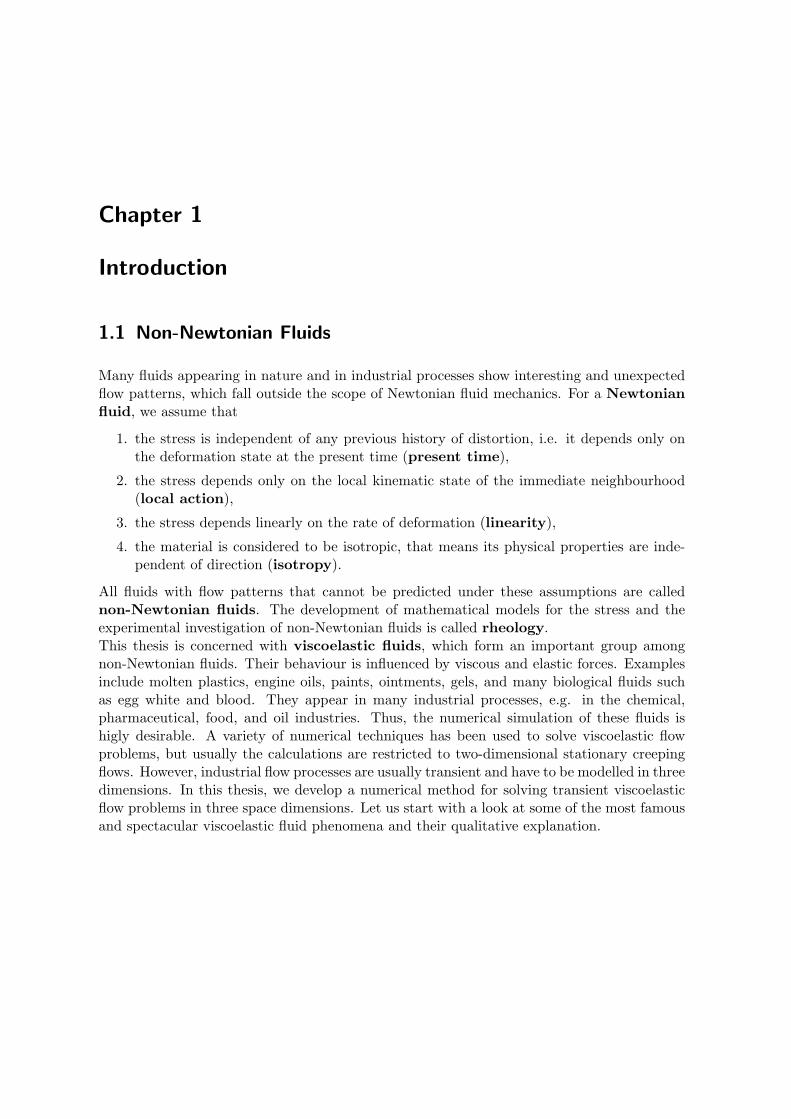
Many fluids appearing in nature and in industrial processes show interesting and unexpectedflow patterns, which fall outside the scope of Newtonian fluid mechanics. For a Newtonianfluid, we assume that
1. the stress is independent of any previous history of distortion, i.e. it depends only onthe deformation state at the present time (present time),
2. the stress depends only on the local kinematic state of the immediate neighbourhood(local action),
3. the stress depends linearly on the rate of deformation (linearity),
4. the material is considered to be isotropic, that means its physical properties are inde-pendent of direction (isotropy).
All fluids with flow patterns that cannot be predicted under these assumptions are callednon-Newtonian fluids. The development of mathematical models for the stress and theexperimental investigation of non-Newtonian fluids is called rheology.This thesis is concerned with viscoelastic fluids, which form an important group amongnon-Newtonian fluids. Their behaviour is influenced by viscous and elastic forces. Examplesinclude molten plastics, engine oils, paints, ointments, gels, and many biological fluids suchas egg white and blood. They appear in many industrial processes, e.g. in the chemical,pharmaceutical, food, and oil industries. Thus, the numerical simulation of these fluids ishigly desirable. A variety of numerical techniques has been used to solve viscoelastic flowproblems, but usually the calculations are restricted to two-dimensional stationary creepingflows. However, industrial flow processes are usually transient and have to be modelled in threedimensions. In this thesis, we develop a numerical method for solving transient viscoelasticflow problems in three space dimensions. Let us start with a look at some of the most famousand spectacular viscoelastic fluid phenomena and their qualitative explanation.

2 Chapter 1 Introduction
1.2 Phenomena in Viscoelastic Flows
(a) Weissenberg effect (G. McKinley [48]). (b) Die swell in Newtonian and polymeric liquids(YouTube, Psidot [56]).
Figure 1.1: Normal stress effects.
The basic feature of viscoelastic fluids is the presence of long chain molecules within thefluid. These have to be taken into account in order to describe viscoelastic flow behaviour.The molecular chains affect the surrounding fluid particles, whereas the surrounding particlesdeform the chain molecules. This interplay of differently shaped and sized particles givesrise to typical macroscopic viscoelastic fluid phenomena. Polymeric liquids, which arecharacterized by very long molecular chains, show viscoelastic effects in a distinctive manner.Thus, they are used in all experiments introduced in this section.We start with one of the most striking viscoelastic phenomena: the rod-climbing or Weis-senberg effect. Experimentally, a rotating rod is inserted into a beaker filled with liquid. Ina Newtonian fluid, the rotating motion generates a centrifugal force which pushes the liquidoutward and the free surface dips near the rod. In contrast, in viscoelastic fluids, the freesurface rises and the fluid climbs up the rod (see Figure 1.1(a)). The rod-climbing is causedby tension along the concentric streamlines, which leads to a force pushing the fluid inward.This tension force arises from the deformation of the molecular chains. The molecular chainsare aligned and stretched out with the flow direction by the drag forces exerted on them bythe surrounding fluid. Their natural tendency to retract from this stretched configurationgenerates the tension, which tries to reduce the length of the streamlines, hence pulling theliquid towards the rod. This tension is usually referred to as a “normal stress”.Another effect linked to the normal stress is die swell. When a fluid is forced out of the orificeof a syringe, the jet of extrudate swells, i.e. it expands radially to a diameter greater thanthat of the orifice. Newtonian fluids exert this effect as well, but the increase in diameteris considerably greater for polymeric fluids. This is again due to the tension along thestreamlines, which is generated by the shearing motion, which stretches the molecular chainsinside the orifice. When the fluid exits the orifice, the tension is relieved, causing the jet toshrink in the longitudinal direction and expand in the transverse direction. See Figure 1.1(b)for a contrast between a Newtonian and a polymeric die swell.The normal stress can become very large and can even enable a fluid to flow against gravityas observed in the tubeless syphon experiment, illustrated in Figure 1.2. In the experiment,a nozzle is dipped into a dish of a polymeric liquid and is sucked into the syringe. Then, the

1.3 About this Thesis 3
Suction
MolecularElongation
Gravity
.(a) Molecular explanation. (b) Tubeless syphon effect (YouTube, Psidot [57]).
Figure 1.2: Tubeless syphon.
syringe is raised above the free surface under continuous pulling. In contrast to Newtonianfluids, where the jet of fluid would immediately break, the polymeric fluid continues toflow into the syringe against gravity. The strong and fast stretching of the fluid causes themolecular chains to stretch very rapidly generating a huge normal stress strong enough topull the liquid out of the dish. A schematic sketch of the stretching of the molecular chainsis presented in Figure 1.2(a).
1.3 About this Thesis
The main aim of this thesis is to develop a numerical method for solving transient viscoelasticflow problems in three space dimensions. The first step toward the numerical simulation ofviscoelastic flows is to make a choice on the mathematical model to describe viscoelasticity.
Mathematical Modelling of Viscoelastic Fluids
As observed in the previous section, any mathematical model of viscoelasticity has to takethe molecular chains and their interaction with the flow into account. Since the molecularstructure of a fluid can be very complex and differs enormously from one material to an-other, it is impossible to find a general model suitable for the description of all classes ofviscoelastic materials. Therefore, there exists a huge amount of different models in literature.This forces us to make a choice on the mathematical model and therewith on the kinds offluids, we wish to describe. In this thesis, we give an overview over the most famous modelsin viscoelasticity. Since the mathematical description of viscoelasticity is a difficult task, wegive a detailed introduction to the mathematical modelling starting with the basic definitionsof shear-rate dependent viscosity, normal stress differences and elongational viscosity. Theseterms describe important material properties and offer a way to categorize materials. Forexample, for Newtonian fluids both the shear-rate dependent viscosity and the elongational

4 Chapter 1 Introduction
viscosity are constant and there are no normal stress differences, but for viscoelastic fluidsthe viscosities are functions of the deformation rate and normal stress differences occur.In a next step, we investigate the viscosity functions and normal stress differences in order tocategorize the introduced models according to the classes of fluids they describe, as well as toshow their respective advantages and disadvantages. Therefore, we solve the model equationsfor two simple flows (the steady shear flow and the uniaxial extension) by Newton’s methodand plot the viscosity functions and normal stress differences.Our general overview commences with linear viscoelasticity models and their generalizationinto a 3D tensor formulation. Then, we present the basic ideas for models derived from molec-ular theories. Among these models, we focus on the derivation of the Oldroyd-B equationsto model dilute polymer solutions and the derivation of the Phan-Thien Tanner equationsto model polymer melts and concentrated solutions. We derive the Oldroyd-B model fromthe notion of elastic dumbbells consisting of two beads connected by a spring, which swimin a Newtonian fluid. To obtain the expression for the stress tensor, we deduce the equationof motion for the dumbbell and obtain a Fokker-Planck equation for the distribution of theend-to-end vector of such an elastic dumbbell. Then, we acquire the equation for the stresstensor through averaging of the forces transmitted from the dumbbells to the fluid. After-wards, we derive the Phan-Thien Tanner equations from a network of molecular chains thatare linked at temporary junctions. Here, we use the equation for the non-affine motion of thenetwork and the Liouville equation for the loss and creation rates of the junctions to obtainthe equation for the stress tensor. After investigating these models in two simple flows, weconclude the overview by a table describing the properties of all introduced models in termsof viscosities and normal stress differences as described above.We choose the Oldroyd-B equations and both the exponential form and the linear form of thePhan-Thien Tanner equations including the prediction of non-affine motion and a Newtoniancontribution to the stress tensor to model viscoelasticity. This enables us to simulate a widevariety of viscoelastic fluids including dilute polymer solutions, polymer melts and concen-trated solutions. Furthermore, both the Oldroyd-B and the Phan-Thien Tanner models aresophisticated models describing viscoelastic flow behaviour quite accurately.
Numerical Method
After choosing the viscoelastic models, we can proceed to discuss their numerical solution.In order to simulate the flow of a viscoelastic fluid, we need the continuity equation, themomentum equation and the viscoelastic model equation. We assume that the fluids areincompressible and that thermal effects can be neglected. Both the Oldroyd-B and the Phan-Thien Tanner equations have a Newtonian contribution to the stress tensor so that theirinsertion into the momentum equation results in
ρDuDt
= −∇p+ η0β∆u + div τττ , (1.1)
where ρ is the density of the fluid, η0 is the total viscosity ( = Newtonian viscosity + polymericviscosity), β is the ratio of the Newtonian viscosity to the total viscosity, u is the velocity,p is the pressure and τττ is the elastic stress tensor described by the Oldroyd-B or Phan-Thien Tanner equations. The momentum equation (1.1) is an extension of the Navier-Stokesequations: the diffusive terms are scaled through the parameter β and the divergence of the

1.3 About this Thesis 5
elastic stress tensor is added. Therefore, we can use a Navier-Stokes solver as the basis forour numerical solution. We use the CFD package NaSt3DGP [1], which contains a fullyparallelized, three-dimensional Navier-Stokes solver developed at the Institute for NumericalSimulation in the research group of Prof. Michael Griebel. In summary, we implement thefollowing modifications and extensions into NaSt3DGP in order to include the Oldroyd-B andPTT equations:
We choose a proper spatial discretization point for the elastic stress tensor components.
We solve the Oldroyd-B and Phan-Thien Tanner equations and implement appropriateboundary and initial conditions for the six elastic stress tensor components (the elasticstress tensor is symmetric, therefore we have to calculate only six components).
We extend the Navier-Stokes equations to the momentum equation (1.1).
We extend the temporal discretization scheme to solve the coupled system of equationsincluding the viscoelastic stress equations.
We parallelize all modifications to accelerate the computation.
We find appropriate ways to visualize the stress tensor.
Before, we implement any equations, we have to choose the discretization points of the stresstensor components. NaSt3DGP uses a staggered grid approach, where the pressure is dis-cretized at the centre of the cells, while the velocities are discretized at the cell sides. How-ever, it remains to locate the stress tensor components on this grid. There are mainly twoapproaches in literature: one, which discretizes the normal stress tensor components in themiddle of the cells and the shear stress components at the vertices of the cells and the other,which discretizes all stress components in the middle of the cells. We decided to discretize allstress tensor components in the middle of the cells, which avoids having an unknown locatedat a cell vertex, that may happen to be at a geometric singularity.Then, we discretize the spatial derivatives in the Oldroyd-B and Phan-Thien Tanner equa-tions by central differences except for the convective terms, which we discretize by higherorder methods. Here, NaSt3DGP offers several higher order methods including the VONOSscheme and the WENO scheme. To our knowledge, the WENO scheme has not yet been usedin the simulation of viscoelastic fluids. In most published work the first order upwind methodor the QUICK scheme are used. However, these scheme have some severe disadvantages. Thefirst order upwind method introduces a lot of numerical diffusion polluting the results and theQUICK scheme produces unphysical oscillations. Therefore, the usage of more sophisticatedhigher order methods such as the WENO scheme can produce better results. Moreover, weimplement Dirichlet, homogeneous Neumann and no-slip boundary conditions for the stresstensor components. In a next step, we extend the Navier-Stokes equations by the parameterβ and discretize the divergence of the elastic stress tensor by central differences.Of course, also the temporal discretization scheme has to be modified in order to include theviscoelastic model equations. For the temporal discretization NaSt3DGP employs a Chorin-type projection method and a semi-implicit projection method with implicit treatment of thediffusive terms developed by Klitz [42]. We extend both projection methods. Therefore, weadvance the Oldroyd-B and Phan-Thien Tanner equations explicitly in time by the Eulermethod to obtain the stress components at the new time-step. These stress tensor compo-nents are then used in the calculation of the intermediate velocity field. Furthermore, we haveto include a time-step restriction arising from the explicit treatment of the viscoelastic model

6 Chapter 1 Introduction
equations.Since we need to solve the governing equations for ten unknowns: three velocity components,the pressure and six stress tensor components at each time-step, the computation of three-dimensional transient viscoelastic flows is a huge computational task, especially for complexflow situations. This is one reason why most of the numerical methods currently available areonly implemented for 2D cases. Therefore, we have to accelerate our computations. We canreduce the total computing time by parallelization, which divides the work between severalprocessors. We parallelized all our extensions and we tested the parallelization by efficiencyand speed-up computations. The tests show excellent results even for large processor numberstreating very small domains.To visualize the stress tensor, we compute a flow directed decomposition of the stress tensorinto shear and normal stress to obtain a physically meaningful stress measure in complexflows [10]. These values can be used to calculate a principal stress. We implement differentfile writing routines for the stress tensor components and the computed shear, normal andprincipal stress to visualize the data with Matlab and ParaView [32].
Validation and Results
To validate our implementation, we investigate
the numerical approximation of the analytical solution for transient plane Poiseuille flowof an Oldroyd-B fluid,
the order of convergence for a three-dimensional gravity driven flow through an infiniterectangular channel.
We implement and parallelize the analytical solution for the plane Poiseuille flow of anOldroyd-B fluid for both the velocity and stress tensor components into NaSt3DGP in orderto compare our numerical results with the transient analytical solution. We find a very goodagreement between the transient analytical solution and the numerical solution for the veloc-ities and stress tensor components. Further, we find that the numerical solution convergesquadratically to the steady state analytical solution with mesh refinement. To validate thecode in three space dimensions for both the Oldroyd-B and the Phan-Thien Tanner equa-tions, we carry out a convergence study for the three-dimensional gravity driven flow throughan infinite rectangular channel. We find the fantastic result of quadratic convergence for allcomponents.Furthermore, we examine
the flow through a three-dimensional rectangular channel,
the flow over a hole,
the Karman vortex street behind an inclined plate
and compare the results for the different models. For the flow through a three-dimensionalrectangular channel, we plot and compare the velocity and stress tensor components for thedifferent models. Then, we examine the flow over a hole and observe an asymmetric vortexstructure for the Oldroyd-B fluid and the PTT fluids, as seen in experiments with viscoelasticfluids. Subsequently, we analyze the stress behaviour on the corner singularities of the flowfor the different models and find very steep stress gradients for the Oldroyd-B model, while

1.4 Outline 7
the stress gradients for the Phan-Thien Tanner models are much less problematic. Finally, weinvestigate the Karman vortex street behind an inclined plate for the different models. We areable to observe different vortex stretching behaviour and suppression of velocity fluctuationsas seen in laboratory experiments. To our knowledge, the Karman vortex street behind aninclined plate, has not yet been numerically investigated for viscoelastic flows.
1.4 Outline
This thesis is organized as follows:Chapter 2 gives a short overview over the basic principles of continuum mechanics neededfor the mathematical description of fluid flows.Chapter 3 introduces the most famous models describing viscoelasticity. We start with thedefinition of the shear-rate dependent viscosity, normal stress differences and elongational vis-cosity. Then, we present the linear viscoelasticity models, explain the terms relaxation timeand fading memory and discuss their generalization into a 3D tensor formulation. In a nextstep, we introduce the basic ideas for models derived from molecular theories and discuss indetail the derivation of the Oldroyd-B equations and of the Phan-Thien Tanner equations.Afterwards, we investigate the behaviour of the Oldroyd-B model and the Phan-Thien Tan-ner model in simple flows, discuss their advantages and disadvantages, and consider the fluidsthey describe. Finally, we present an overview over all the models introduced.Chapter 4 gives the full set of equations necessary to describe viscoelastic flows. We discusstheir non-dimensionalization and the boundary conditions needed in order to solve them.The non-dimensionalization introduces the Weissenberg number, which is associated witha problem called the high Weissenberg number problem (HWNP) describing the numericalbreakdown beyond some critical value of the Weissenberg number. We will discuss some ofthe important aspects causing this problem.Chapter 5 deals with the numerical solution of the governing equations. First, we presenta Chorin-type explicit project method. Then, we discuss the time-step restrictions resultingfrom the explicit treatment of the equations. Since the time-step restriction for the diffusiveterms leads to very small time-steps for low Reynolds number flows, we also introduce a semi-implicit projection method. Afterwards, we discuss the spatial discretization on a staggeredgrid and the discrete boundary values.Chapter 6 discusses a parallelization strategy by domain decomposition, which enables us toaccelerate our computations. We measure the acceleration in terms of speed-up and efficiencyand obtain very good results.Chapter 7 contains our numerical results. We validate our code by the investigation ofthe numerical approximation of the analytical solution for transient plane Poiseuille flow ofan Oldroyd-B fluid and by a convergence study on a three-dimensional gravity driven flowthrough an infinite rectangular channel. Furthermore, we examine the flow through a three-dimensional rectangular channel, the flow over a hole and the Karman vortex street behindan inclined plate for different models and compare their results.Chapter 8 concludes this thesis by a summary of its main results and a presentation ofvarious possibilities for future research.The Appendix gives the components of the set of equations and the derivation of the ana-lytical solution of the plane Poiseuille flow of an Oldroyd-B fluid for the stress components.

8 Chapter 1 Introduction

Chapter 2
Review of Continuum Mechanics
In this chapter, we give a short overview over the basic principles of continuum mechanicsneeded for the mathematical description of fluid flows. The presentation is based on Phillipsand Owens [50], Chorin and Marsden [16], Bohme [12], Phan-Thien [54] and Tanner [67].
2.1 Kinematics
2.1.1 Velocity and Acceleration
Let V ⊂ R3 be a region filled with a fluid consisting of particles. Consider a fixed Cartesianframe of reference with orthonormal base vectors e1, e2 and e3. The position of a particle isthen given by the position vector
x(t) = (x(t), y(t), z(t)) ≡ x(t)e1 + y(t)e2 + z(t)e3 (2.1)
at some time t. Then we define the velocity of the particle as
u(x(t), t) =dx(t)dt
. (2.2)
The acceleration of the fluid particle is given by
a(x(t), t) =d2
dt2x(t) =
d
dtu(x(t), t). (2.3)
By the chain rule, this becomes
a(x(t), t) =∂u∂t
+∂u∂x
dx
dt+∂u∂y
dy
dt+∂u∂z
dz
dt=
∂
∂tu + (u · ∇)u. (2.4)
Definition 2.1 [material Derivative]We define the material derivative to be the operator
D
Dt:=
∂
∂t+ u · ∇. (2.5)
The material derivative differs from the local time derivative ∂∂t in the part u · ∇, which
originates from the motion of the particle. Thus, we see that the material derivative includesthe motion of the particle.

10 Chapter 2 Review of Continuum Mechanics
As seen above, the acceleration of a fluid particle is given by the sum of the local timederivative and the convective term u · ∇u.
Definition 2.2 [Velocity Gradient Tensor]The expression ∇u is a second-order tensor containing the velocity field derivatives. There-fore, we call it the velocity gradient tensor. It is given by
∇u =
∂u∂x
∂u∂y
∂u∂z
∂v∂x
∂v∂y
∂v∂z
∂w∂x
∂w∂y
∂w∂z
. (2.6)
2.1.2 Deformation and Vorticity
We can decompose the velocity gradient tensor into a symmetric part D (i.e. DT = D)and an anti-symmetric part W (i.e. WT = −W), as
∇u = D + W.
Definition 2.3 [Rate of Deformation Tensor]The symmetric part is called the rate of deformation tensor and it is given by
D :=12
(∇u +∇uT ) =
∂u∂x
12(∂u∂y + ∂v
∂x) 12(∂u∂z + ∂w
∂x )12(∂u∂y + ∂v
∂x) ∂v∂y
12(∂v∂z + ∂w
∂y )12(∂u∂z + ∂w
∂x ) 12(∂v∂z + ∂w
∂y ) ∂w∂z
. (2.7)
Definition 2.4 [Vorticity Tensor]The anti-symmetric part is called the vorticity tensor and it is given by
W :=12
(∇u−∇uT ) =
0 −12( ∂v∂x −
∂u∂y ) 1
2(∂u∂z −∂w∂x )
12( ∂v∂x −
∂u∂y ) 0 −1
2(∂w∂y −∂v∂z )
−12(∂u∂z −
∂w∂x ) 1
2(∂w∂y −∂v∂z ) 0
. (2.8)
We will now discuss their physical interpretation. Let r denote the position of a particleand r + dr the position of a neighbouring particle at a small distance dr as illustrated inFigure 2.1(a). Then, we obtain by Taylor’s theorem
u(r + dr) = u(r) +∇u(r)dr.
With u(r) = dr/dt and u(r + dr) = d(r + dr)/dt, we get
d(dr)dt
= ∇u(r)dr. (2.9)
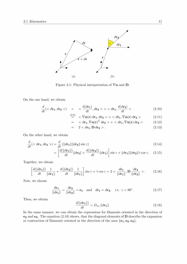
Therefore, we see that the velocity gradient tensor ∇u transforms the filament dr into itstime derivative. For the physical interpretation of the rate of deformation tensor D, we taketwo filaments dr1 and dr2 (see Figure 2.1(b)). Let (90−γ) be the angle between them. Nowwe examine the time derivative of the standard scalar product < ., . > of these two filaments.
2.1 Kinematics 11
r
r + dr
dr
(a)
r
dr1
dr2
γ
(b)
Figure 2.1: Physical interpretation of ∇u and D.
On the one hand, we obtain
d
dt(< dr1, dr2 >) = <
d(dr1)dt
, dr2 > + < dr1,d(dr2)dt
> (2.10)
(2.9)= < ∇u(r) dr1, dr2 > + < dr1,∇u(r) dr2 > (2.11)= < dr1,∇u(r)T dr2 > + < dr1,∇u(r) dr2 > (2.12)= 2 < dr1,D dr2 > . (2.13)
On the other hand, we obtain
d
dt(< dr1, dr2 >) =
d
dt(‖dr1‖‖dr2‖ sin γ) (2.14)
=[d(‖dr1‖)
dt‖dr2‖+
d(‖dr2‖)dt
‖dr1‖]
sin γ + ‖dr1‖‖dr2‖γ cos γ. (2.15)
Together, we obtain[d(‖dr1‖)
dt
1‖dr1‖
+d(‖dr2‖)
dt
1‖dr1‖
]sin γ + γ cos γ = 2 <
dr1
‖dr1‖,D
dr2
‖dr2‖> . (2.16)
Now, we choose
dr1
‖dr1‖=
dr2
‖dr2‖= e1 and dr1 = dr2, i.e. γ = 90. (2.17)
Then, we obtaind(‖dr1‖)
dt= Dxx ‖dr1‖. (2.18)
In the same manner, we can obtain the expressions for filaments oriented in the direction ofe2 and e3. The equation (2.18) shows, that the diagonal elements of D describe the expansionor contraction of filaments oriented in the direction of the axes e1, e2, e3.
12 Chapter 2 Review of Continuum Mechanics
h1
h2h3
h∗1
h∗2h∗3
time t time t∗ = t+ ∆t
(a) h∗1 = h1(1 +Dxx∆t), h∗2 = h2(1 +Dyy∆t), h∗3 = h3(1 +Dzz∆t)
γ
time t time t∗ = t+ ∆t
(b) Dxy = γ/2
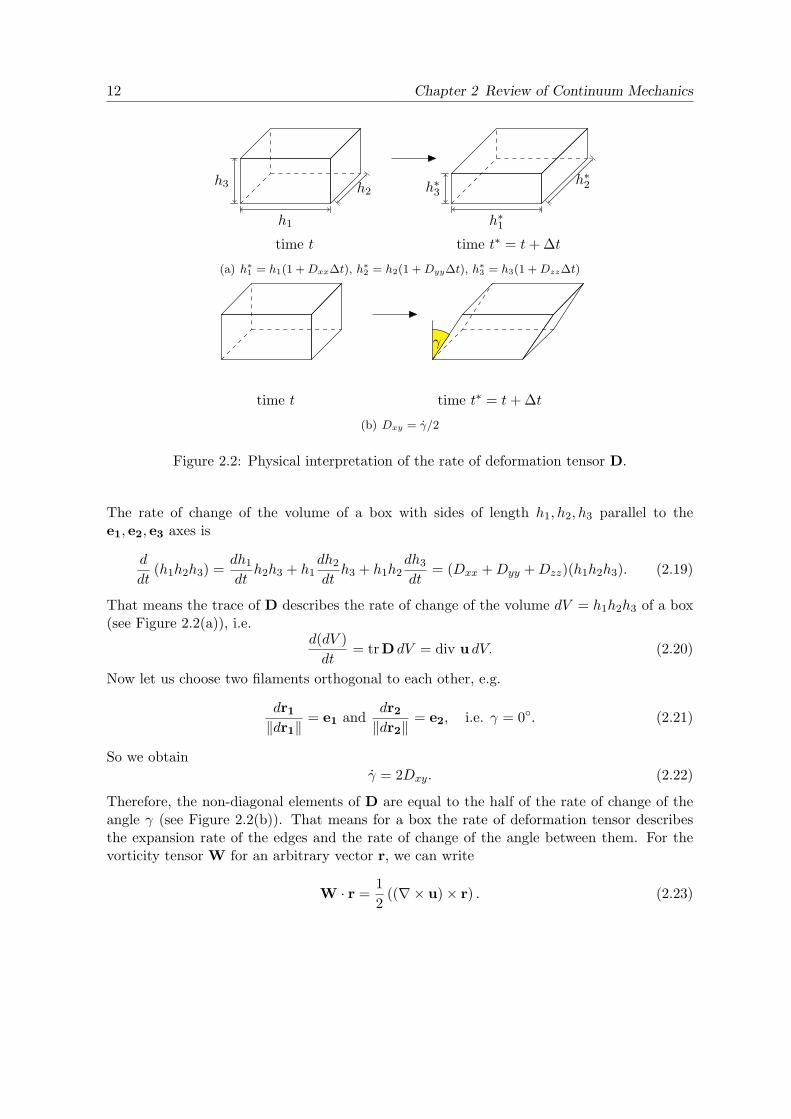
Figure 2.2: Physical interpretation of the rate of deformation tensor D.
The rate of change of the volume of a box with sides of length h1, h2, h3 parallel to thee1, e2, e3 axes is
d
dt(h1h2h3) =
dh1
dth2h3 + h1
dh2
dth3 + h1h2
dh3
dt= (Dxx +Dyy +Dzz)(h1h2h3). (2.19)
That means the trace of D describes the rate of change of the volume dV = h1h2h3 of a box(see Figure 2.2(a)), i.e.
d(dV )dt
= tr D dV = div u dV. (2.20)
Now let us choose two filaments orthogonal to each other, e.g.
dr1
‖dr1‖= e1 and
dr2
‖dr2‖= e2, i.e. γ = 0. (2.21)
So we obtainγ = 2Dxy. (2.22)
Therefore, the non-diagonal elements of D are equal to the half of the rate of change of theangle γ (see Figure 2.2(b)). That means for a box the rate of deformation tensor describesthe expansion rate of the edges and the rate of change of the angle between them. For thevorticity tensor W for an arbitrary vector r, we can write
W · r =12
((∇× u)× r) . (2.23)

2.1 Kinematics 13
For filaments, we can obtain from (2.9) the following relation
d(dr)dt
=(∇× u)
2× dr. (2.24)
That means the vorticity tensor W describes the rotation of a filament dr with angularvelocity (∇× u)/2.
2.1.3 Strain
O
time ttime s
x
dxP
Q
r
drPQ
Figure 2.3: Motion of a body from time t to time s.
The quantities D and W are sufficient for Newtonian fluid mechanics, but additional quanti-ties are required to describe solid materials or materials with memory. Looking at Figure 2.3,if P and Q are neighbouring points separated by a small distance dx at time t and by adistance dr at time s. Let r(x, t, s) denote the position at time s of the fluid particle P , whichoccupies position x at time t. By definition, we have
r(x, t, t) = x. (2.25)
As we move to the neighbouring particle Q the mapping r(x, t, s) means that the relationbetween dr and dx is:
dri =∂ri∂x1
dx1 +∂ri∂x2
dx2 +∂ri∂x3
dx3 with ri = ri(xi, t, t′) , i = 1, 2, 3. (2.26)
This gives us the possibility to define the following strain tensor.
Definition 2.5 [deformation gradient tensor]We define the deformation gradient tensor F relating dr and dx as
dr = F(x, t, s)dx, (2.27)
i.e.Fij =
∂ri∂xj
. (2.28)

14 Chapter 2 Review of Continuum Mechanics
Unfortunately, the deformation gradient tensor is not suitable for the description of strain,because it violates the principle of frame indifference. This principle states that a physicalprocess is invariant under changes of observers. The deformation gradient tensor is F = I foruniform translations, but F 6= I for rigid rotations. That is why we choose to investigate themagnitudes of dr and dx. We can form ‖dr‖2 and find
‖dr‖2 = dr12 + dr2
2 + dr32 = drTdr = (Fdx)TFdx = dxT (FTF)dx. (2.29)
Definition 2.6 [Cauchy-Green strain tensor]The quantity FTF is called the Cauchy-Green strain tensor.
C(x, t, s) := FT (x, t, s)F(x, t, s) with s ∈ (−∞, t]. (2.30)
The Cauchy-Green strain tensor represents the strain history of filaments of the material.Note that C(x, t, t) = I.
2.2 Stress and Body Forces
We recognize two types of forces acting on an infinitesimal fluid element, which occupies avolume V at some time (see Figure 2.4). One, due to the action-at-a-distance type of forcessuch as gravitation and electromagnetic forces, can be expressed as force per unit mass, andis called body force; the other, due to the direct action across the boundary surface S, iscalled the surface force. To describe the body force, we assume that the fluid element has
n
t dSf
dS
V
dV
Figure 2.4: Stress and body force definition.
a well-defined mass density ρ. The mass of the fluid element with volume V is then givenby
m =∫V
ρ dV. (2.31)

2.2 Stress and Body Forces 15
So that the total body force acting on the volume V is given by
Fb =∫V
ρb dV, (2.32)
where b is the body force per unit mass.To describe the surface force, let us consider a small surface element of area dS with anoutward pointing unit normal vector n. Then the total surface force acting on S is given by
Ft =∫S
t dS, (2.33)
where t is the force per unit area acting on the surface and is called the stress vector. Theclear isolation of surface forces in a continuum is usually attributed to Cauchy.Then the total force experienced by the fluid occupying V will now be
total force =∫V
ρb dV +∫S
t dS. (2.34)
Theorem 2.7 [Existence and Symmetry of the Stress Tensor]Let V ⊂ R3 be some bounded region and let t be the stress vector defined above. Then thereexists a second-order stress tensor σσσ such that throughout V
(i)t = σσσ · n, (2.35)
i.e. the stress tensor σσσ can be seen as a linear mapping of the unit normal vector ninto the stress vector t.
(ii)σσσ is symmetric. (2.36)
σσσ is called the Cauchy stress tensor.
Proof. See e.g. Phillips and Owens [50], p. 361ff.
Notation: The components of the stress tensor are usually denoted as seen in Figure 2.5 by
σσσ =
σxx σxy σxzσyx σyy σyzσzx σzy σzz
, (2.37)
where the σxx, σyy, σzz components are called normal stresses and σxy = σyx, σxz =σzx, σyz = σzy are called shear stresses.

16 Chapter 2 Review of Continuum Mechanics
z
xy
σzy
σxy σyy
σzz
σxzσyz
σzx
σxx
σyx
Figure 2.5: Notation used for the stress tensor.
Definition 2.8 [deviatoric stress/extra-stress tensor]For fluids, we decompose the Cauchy stress tensor into one from the rate of deformationindependent spherical-symmetrical pressure part and the deviatoric stress or more generallyextra-stress tensor part T.
σσσ = −pI + T. (2.38)
2.3 Conservation Laws
The motion of every fluid is governed by the conservation of mass and momentum, and ifthermal effects are important, the balance of energy. In this thesis, we will be only concernedwith purely mechanical problems, where we assume a constant temperature. We will alsoassume that the fluids are incompressible, i.e. Dρ
Dt = 0. In order to proceed, we first needthe Reynolds transport theorem, which enables us to compute the rate of change of certainvolume integrals.
Theorem 2.9 [Reynolds transport theorem]Let V (t) a region filled with a fluid and let f(x, t) be a scalar or vector function defined overV (t). Then
d
dt
∫V (t)
f dV =∫V (t)
(Df
Dt+ fdiv u
)dV. (2.39)
Proof. See e.g. Phan-Thien [54], p.49
2.3.1 Conservation of Mass
The mass in the volume V (t) is conserved at all time, i.e.
d
dt
∫V (t)
ρ dV = 0, (2.40)

2.3 Conservation Laws 17
where ρ(x, t) is the density field at time t. By Reynolds transport theorem (2.39), we get∫V (t)
(Dρ
Dt+ ρdiv u
)dV = 0. (2.41)
Since the volume V (t) is arbitrary, we deduce that
Dρ
Dt+ ρ · div u = 0. (2.42)
For incompressible fluids (i.e.Dρ
Dt= 0), we get
div u = 0. (2.43)
2.3.2 Conservation of Linear Momentum
By (2.33) the total force acting on a volume element is given by
total force =∫V
ρb dV +∫S
t dS. (2.44)
By Newton’s second law (force = mass · acceleration), (2.35) and the divergence theorem(DT), we are led to∫
V
ρDuDt
dV =∫V
ρb dV +∫S
σσσ · n dS DT=∫V
ρb dV +∫V
div σσσ dV. (2.45)
With equation (2.38), we obtain∫V
ρDuDt
dV =∫V
ρb dV −∫V
∇p dV +∫V
div T dV. (2.46)
Since the integrand is continuous on an arbitrary V , the conservation of linear momentumbecomes
ρDuDt
= −∇p+ div T + ρb. (2.47)


Chapter 3
Constitutive Equations
To complete the mathematical formulation, we need to relate the extra-stress tensor T tothe motion. These supplementary relations, which are called the constitutive equationsor the rheological equations of state, differentiate one material from another. The firststep in evaluating constitutive models is to consider their predictions in a number of simpleflows. We will look at two simple types of flows: steady shear flow and uniaxial extensionalflow. This will lead us to the definition of shear-dependent viscosity, normal stress differencesand elongational viscosity. This chapter is based on the books of Tanner [67], Bohme [12],Bird [6, 7], Renardy [61] and Owens [50].
3.1 Simple Flows, Viscosities and Stress Differences
3.1.1 Steady Shear Flow and Viscometric Functions
x
y
h
u
Figure 3.1: Steady shearing.
Consider a fluid between two infinite paralleled plates separated by a distance h as shownin Figure 3.1. Now, suppose that the top plate moves with a constant velocity u in the x-direction. This flow is called steady shear flow or viscometric flow. The velocity field isgiven by
u = (u(y), 0, 0).
Consequently, the velocity gradient and the rate of deformation tensor are
∇u =
0∂u(y)∂y
0
0 0 00 0 0
; 2D =
0
∂u(y)∂y
0
∂u(y)∂y
0 0
0 0 0
. (3.1)

20 Chapter 3 Constitutive Equations
The quantity
γ :=∂u(y)∂y
, (3.2)
is known as the shear rate. If we consider an isotropic material, the zx- and zy-componentsof stress must be zero. This can be seen in the following way. Consider two observers; one inour standard Cartesian frame and one in a coordinate frame rotated 180 about the z-axis asshown in Figure 3.2. Because both observers see the same flow, the stresses investigated by
y
xz σyz
σxz
1 2
y
x z
σyz
σxz
Figure 3.2: Two observers.
them must be the same in an isotropic material. Therefore, we must have σxz = σyz = 0 andthe stress tensor has the form
σσσ =
σxx σxy 0σxy σyy 00 0 σzz
. (3.3)
When a viscoelastic liquid is brought from rest into a state of steady shearing motion, a time-dependent shear stress is built up. However, if the shearing motion continues at a constantrate, the shear stress approaches a steady-state value that depends only on the shear rate.
Definition 3.1 [viscometric functions]The ratio of the shear stress σxy to the shear rate is a function
η(γ) =σxyγ
(3.4)
called the (shear-rate dependent) viscosity. The shear viscosity η is typically a mono-tonically decreasing function of shear rate that tends to some limit η∞ for very high-shearrates. Such fluids are termed shear-thinning. At low shear rates, the viscosity approachesa constant value
η0 = limγ→0
η(γ),
which is called zero-shear-rate-viscosity.The two independent differences
N1(γ) := σxx − σyy, (3.5)N2(γ) := σyy − σzz (3.6)

3.1 Simple Flows, Viscosities and Stress Differences 21
are called the first and second normal stress differences respectively. Polymeric fluidsusually have non-zero normal stress differences, where the first normal stress difference ispositive, the second normal stress difference is negative and its absolute value is much smallerthan that of N1.
3.1.2 Steady Uniaxial Extensional Flow and Elongational Viscosity
x
z
y
Fluid element attime t1
Fluid element attime t2 > t1
Figure 3.3: Steady uniaxial extensional flow.
Suppose that a rod of material is being extended homogeneously along its x-axis, so that eachpart of the rod is stressed uniformly as shown in Figure 3.3. We suppose that the constant rateof elongation ∂u/∂x(≡ ε) is independent of x. For an incompressible fluid, mass conservationand axial symmetry then demand that ∂v/∂y = ∂w/∂z = −ε/2. Thus, the velocity in asteady elongational flow is given by
u = (εx,− ε2y,− ε
2z). (3.7)
Consequently, the velocity gradient tensor and the rate of deformation tensor are equal and
∇∇∇u = D =
ε 0 00 − ε
2 00 0 − ε
2
. (3.8)
All shear stress components are zero and σyy = σzz by symmetry. Shear stresses would leadto an angle change in volume elements. Therefore, the stress tensor becomes
σσσ =
σxx 0 00 σyy 00 0 σyy
. (3.9)
The stress response is then completely defined by the dependence of σxx−σyy on the constantrate of extension ε.
Definition 3.2 [Elongational Viscosity]The ratio of the stress difference σxx − σyy to the elongation rate ε
ηE(ε) =σxx − σyy
ε, (3.10)

22 Chapter 3 Constitutive Equations
is called elongational or extensional viscosity. For polymeric fluids, the elongationalviscosity is usually seen to increase as the elongation rate is increased. This behaviour istermed extensional-thickening. The ratio between the extensional viscosity and the shearviscosity is called Trouton ratio
Trouton ratio =ηE(ε)η(γ)
. (3.11)
3.2 The Newtonian Fluid
The constitutive law for a Newtonian fluid is given by
T = 2η0D. (3.12)
This constitutive relation reflects the four assumptions introduced in Section 1.1. As seen inSection 2.1.2 the rate of deformation tensor D contains information about the deformationrate at the present time at a local point. It is symmetric, which means it is suitable for thedescription of isotropic materials. In the relation, we assume that the extra stress T dependslinearly on the rate of deformation D. The proportionality coefficient η0 is called the viscos-ity. This law shows that the viscosity, i.e. the friction of particles at the molecular level, isuniquely responsible for the existence of extra stresses.Substituting equation (3.12) into the momentum equation (2.47) leads in the case of incom-pressible flow to the Navier-Stokes equations
ρDuDt
= −∇p+ η0∆u + ρb. (3.13)
For steady simple shear flow (see Section 3.1.1), the stress tensor of a Newtonian fluid be-comes
σσσ =
−p η0γ 0η0γ −p 00 0 −p
. (3.14)
Therefore, a Newtonian fluid has a constant shear viscosity η0, i.e. it is not shear-thinningand it has zero first and second normal stress differences. For steady uniaxial elongation (seeSection 3.1.2), we obtain
σσσ =
−p+ 2ηε 0 00 −p− ηε 00 0 −p− ηε
. (3.15)
Therefore, the elongational viscosity
ηE(ε) = 3η0, (3.16)
is three times larger than the shear viscosity, i.e. the Trouton ratio is ηE(ε)/η0 = 3.

3.3 The Generalized Newtonian Fluid 23
3.3 The Generalized Newtonian Fluid
As a first step towards deriving constitutive relations for non-Newtonian fluids, we take theshear-thinning effect into account. Therefore, we abandon the assumption that the extrastress tensor depends linearly on the rate of deformation tensor. To derive a model, which isindependent of the coordinate system, we write the viscosity η as a function of the invariantsof D. We use the symmetry of the rate of deformation tensor by noticing that every symmetricsecond order tensor can be diagonalized and its eigenvalues are guaranteed to be real, i.e.
D =
λ1 0 00 λ2 00 0 λ3
, (3.17)
det(D− λI) = −λ3 + IDλ2 − IIDλ+ IIID = 0, (3.18)
where
ID = Dxx +Dyy +Dzz = tr D, (3.19)
IID = DxxDyy +DyyDzz +DzzDxx −D2xy −D2
xz −D2yz =
12
[(tr D)2 − tr D2], (3.20)
IIID = det D (3.21)
are called the principal invariants of D and they are independent of the coordinate sys-tem. Hence, we obtain the following relation between the extra stress tensor and the rate ofdeformation tensor
T = 2η0(ID, IID, IIID)D. (3.22)
Note that (see Bohme [12])
ID = 0 for incompressible fluids. Then IID ≤ 0 , |IIID| ≤ 23√
3(−IID)
32 .
IIID = 0 for simple shear flow.
This model is only suitable for the description of flows, where elastic effects are negligible andthe shear-thinning effect has a strong influence on the flow behaviour. Its principal usefulnessis for calculating flow rates and shearing forces in steady-state simple shear flow such as tubeflow. The most widely used form of the general viscous constitutive relation is the powerlaw model
T = 2K|IID|(n−1)
2 D, (3.23)
where K and n are positive material parameters. Details on models of this kind can be foundin Macosko [47], Bird [6], Bohme [12] and Owens [50]. As well as the Newtonian fluid, thegeneralized Newtonian fluid has zero first and second normal stress differences, but it showsshear-thinning for n < 1 or shear thickening for n > 1.

24 Chapter 3 Constitutive Equations
3.4 Linear Viscoelasticity
In viscoelastic fluids, the stress depends on the history of the motion and not only on thecurrent motion of the fluid.
3.4.1 Maxwell Model
As a first attempt to obtain a viscoelastic constitutive equation, we consider a spring withspring constant G and a purely viscous dashpot with viscosity η0 in series as seen in Figure 3.4.Such an element is called Maxwell element. The dashpot represents viscous behaviour andthe spring represents elastic behaviour.
γ
γ1
G = η0λ
η0
Figure 3.4: Maxwell model.
The stress T1 in the spring is given by Hooke’s law
T1 = G · (γ − γ1),
where (γ − γ1) is the displacement of the spring. The stress T2 in the dashpot is
T2 = η0γ1,
where γ1 = ∂γ1∂t is the velocity, the rate of change of γ1. Because they are in series, i.e.
T1 = T2 = T , after eliminating γ1, we obtain the Maxwell model
T (t) +η
G
∂T (t)∂t
= η0γ(t). (3.24)
We callλ =
η0
G(3.25)
relaxation time. The general solution to Maxwell’s model is given by
T (t) = K e−tλ +
∫ t
−∞
η0
λe−
(t−t′)λ γ(t′) dt′, (3.26)

3.4 Linear Viscoelasticity 25
where K is the integration constant. If we prescribe that the stress is finite at t′ = −∞, wemust choose K to be zero. Therefore, we obtain the following solution for the stress
T (t) =∫ t
−∞
[η0
λe−
(t−t′)λ
]γ(t′) dt′. (3.27)
This equation shows that the stress is determined by the history of the rate of deformationof γ. The quantity
G(t− t′) =η0
λ· e−
t−t′λ (3.28)
is called relaxation modulus. It is more naturally to express the deformation γ(t) as thedeformation at a past time relative to the configuration of the fluid at the present time t.Therefore, we define
γ(t, t′) :=
t∫t′
γ(t′′)dt′′. (3.29)
Then integration by parts of (3.27) yields
T (t) = −∫ t
−∞
[η0
λ2e−
(t−t′)λ
]γ(t, t′) dt′, (3.30)
where
M(t− t′) := − η0
λ2e−
(t−t′)λ =
dG(t− t′)dt
(3.31)
is called memory function.
Example 3.1: [Stress relaxation after a sudden shearing displacement] To under-stand the meaning of the relaxation modulus G(t− t′) and the relaxation time λ, we examinethe following experiment. Consider a Maxwell fluid at rest between two parallel plates forall times t < 0. At time t = 0, the upper plate is moved slightly in the x-direction (seeFigure 3.5) with displacement angle γ0 1. Then, we keep γ0 constant for all t > 0. Since
x
yu = 0
t < 0
Fluid at rest
x
y
γ0
u = γ0y
t > 0
Stressrelaxation
Figure 3.5: Sudden shearing displacement.
the rate of deformation γ is zero except during the time interval [−ε, ε], we obtain from (3.27)after taking the limit ε→ 0 using L’Hopital’s rule
T (t) = γ0G(t) = γ0η0
λe−
tλ . (3.32)
Thus, we see that the stress T (t) decreases exponentially with the relaxation modulus

26 Chapter 3 Constitutive Equations
G(t) = η0λ e−
tλ (see Figure 3.6) and finally reaches zero, i.e. the fluid relaxes again and
it forgets that a change of motion state had taken place. We thus speak of the ”fadingmemory” of a fluid. The relaxation time is a measure for this fading memory. It describeshow long it takes the fluid to relax and how long the fluid remembers the flow history. It isa material parameter. Even Newtonian fluids show memory effects, but their relaxation timeis very short.
t
γ
γ0
(a) Sudden shear.
t
T/γ0
G(t)
G(0)
λ
(b) Maxwell fluid.
t
T/γ0
G(t)
G(0)
(c) Newtonian fluid.
Figure 3.6: Relaxation modulus and relaxation time.
The behaviour of a viscoelastic fluid depends crucially on how the relaxation time relatesto other time scales relevant to the flow, e.g. the observation time scale of an experiment.If the observation time scale is large compared to the memory of the fluid, then memory isunimportant, and the material responses like a Newtonian fluid. If the observation time scaleis small, memory effects are crucial and the material behaves like an elastic solid. The ratioof the relaxation time to a time scale of the flow is an important dimensionless measure ofthe importance of elasticity
De =relaxation time
characteristic time scale. (3.33)
It is called Deborah number. It is named after the prophetess Deborah in the Old Testa-ment, who said, ”the mountains flowed before the Lord.”

3.4 Linear Viscoelasticity 27
3.4.2 Jeffreys Model
One can easily extend Maxwell’s model to get relations for the stress with other rheologicalproperties. The so-called Jeffreys model is a dashpot and a Maxwell element in parallel. Now,
G = ηλ
ηP
ηS
Figure 3.7: Jeffreys model.
the stress consists of the stress at the viscous dashpot ηN γ and of the stress at the Maxwellelement τ . The two elements are in parallel so the stresses are additive
T (t) = ηS γ + τ, (3.34)τ + λτ = ηP γ. (3.35)
After eliminating variable τ , we obtain the Jeffreys model
T (t) + λT (t) = η0 [γ(t) + λrγ(t)] , (3.36)
where γ(t) = ∂2γ∂t2
, η0 = ηS + ηP is the total viscosity and λr = ηSη0λ is the retardation
time.

28 Chapter 3 Constitutive Equations
3.5 Nonlinear Models
3.5.1 Differential Models
In this section, we will generalize the one-dimensional Maxwell and Jeffreys Model into a 3Dtensor formulation. However, we cannot just use the partial time or material time derivative,because they violate the principle of frame indifference (i.e. the material response must beindependent of the observer) for our tensor formulations. We need an objective time derivativeformulated in a coordinate system, which is embedded in a flowing fluid and deforms withit, so that the coordinates associated with a particular material point do not change in time.Such a coordinate system is called convected coordinate system. Following this approach, wecan define the objective time derivatives
Definition 3.3 [Objective time derivatives]Let A be an arbitrary 3D tensor. Then, we define
Upper convected derivative
∇A :=
DADt−∇u ·A−A · ∇uT (3.37)
is a time derivative in a coordinate system, which stretches and rotates with materiallines.
Lower convected derivative
4A :=
DADt
+∇uT ·A + A · ∇u (3.38)
is a time derivative in a coordinate system, which deforms and rotates with surfaceelements (i.e. with area and direction).
Corotational derivative
A :=
DADt−W ·A + A ·W (3.39)
is a time derivative in a coordinate system, which rotates with material lines, but it doesnot stretch with them.
Rigorous derivations of these derivatives can be found in Joseph [34] or Bird [6]. These threederivatives may be combined in one formula given by
δaAδt
:=DADt−W ·A + A ·W − a(D ·A + A ·D), −1 ≤ a ≤ +1. (3.40)
It contains as special cases the upper convected derivative, if a = 1, the lower convectedderivative, if a = −1, and the corotational derivative, if a = 0, but other values of a leadto frame indifferent time derivatives as well. By using these objective time derivatives andMaxwell’s one-dimensional Model (3.24), we get the following relation between the extra stress

3.5 Nonlinear Models 29
tensor T and the rate of deformation tensor D
T + λδaTδt
= 2η0D, (3.41)
where η is the viscosity of the fluid. Of particular importance is the upper convected versionof the model. The upper convected derivative occurs naturally in the derivation of modelsfrom molecular theories as seen in Section 3.6. The Upper Convected Maxwell (UCM)model is given by
T + λ∇T = 2η0 D. (3.42)
It can be written in the integral form (see e.g. Joseph [34])
T(r, t) = −∫ t
−∞
η0
λ2e−(t−t′)
λ (C−1(r, t, t′)− I) dt′, (3.43)
where C−1 is the inverse of the Cauchy-Green strain tensor introduced in Definition 2.6. Forsteady simple shear flow, i.e. DT
Dt = 0, the UCM equations becomeTxx Txy 0Txy Tyy 00 0 Tzz
− λ0 γ 0
0 0 00 0 0
Txx Txy 0Txy Tyy 00 0 Tzz
+
Txx Txy 0Txy Tyy 00 0 Tzz
0 0 0γ 0 00 0 0
= η0
0 γ 0γ 0 00 0 0
,
so that solving this system yields
Txy = η0γ , Txx = 2η0λγ2 , Tyy = Tzz = 0. (3.44)
Therefore, the viscometric functions are given by
η(γ) =σxyγ
= η0 , N1(γ) = σxx − σyy = 2λη0γ2 , N2(γ) = σyy − σzz = 0. (3.45)
Hence, we see that the UCM model predicts a constant shear-rate viscosity, a quadratic firstnormal stress difference and a zero second normal stress difference. For steady elongationalflow, the equationsTxx 0 0
0 Tyy 00 0 Tzz
− λε 0 0
0 − ε2 0
0 0 − ε2
Txx 0 00 Tyy 00 0 Tzz
+
Txx 0 00 Tyy 00 0 Tzz
ε 0 00 − ε
2 00 0 − ε
2
= η0
ε 0 00 − ε
2 00 0 − ε
2
30 Chapter 3 Constitutive Equations
yield
Txx =2η0ε
1− 2λε, Tyy = Tzz = − η0ε
1 + λε. (3.46)
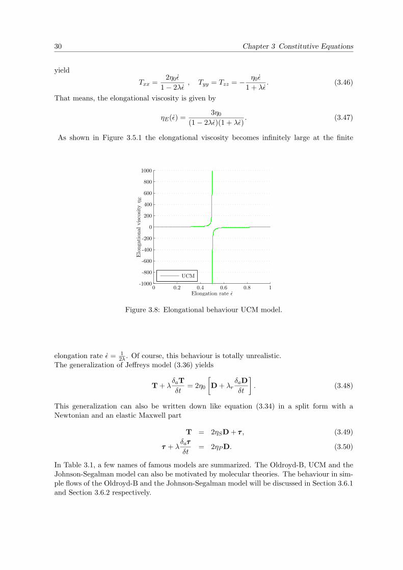
That means, the elongational viscosity is given by
ηE(ε) =3η0
(1− 2λε)(1 + λε). (3.47)
As shown in Figure 3.5.1 the elongational viscosity becomes infinitely large at the finite
Elongation rate ǫ
Elo
ngat
iona
lvi
scos
ity
η E
UCM
0 0.2 0.4 0.6 0.8 1
0
-1000
-800
-600
-400
-200
0
200
400
600
800
1000
Figure 3.8: Elongational behaviour UCM model.
elongation rate ε = 12λ . Of course, this behaviour is totally unrealistic.
The generalization of Jeffreys model (3.36) yields
T + λδaTδt
= 2η0
[D + λr
δaDδt
]. (3.48)
This generalization can also be written down like equation (3.34) in a split form with aNewtonian and an elastic Maxwell part
T = 2ηSD + τττ , (3.49)
τττ + λδaτττ
δt= 2ηPD. (3.50)
In Table 3.1, a few names of famous models are summarized. The Oldroyd-B, UCM and theJohnson-Segalman model can also be motivated by molecular theories. The behaviour in sim-ple flows of the Oldroyd-B and the Johnson-Segalman model will be discussed in Section 3.6.1and Section 3.6.2 respectively.

3.5 Nonlinear Models 31
Model name a λr
Lower Convected Maxwell −1 0Upper Convected Maxwell 1 0Corotational Maxwell 0 0Johnson-Segalman ∈ [−1, 1] 0Oldroyd-A −1 > 0Oldroyd-B 1 > 0
Table 3.1: Famous differential models.
3.5.2 Integral Models
In an integral model, the stress is given in the form of integrals of the deformation history. Themost and widely used incompressible integral models are the Rivlin-Sawyers equations [62]and the K-BKZ equation [37, 5]. These are
K-BKZ equation
T(t) = −∫ t
−∞
[∂V (t− t′, I1, I2)
∂I1(C−1(x, t, t′)− I) +
∂V (t− t′, I1, I2)∂I2
(C(x, t, t′)− I)],
(3.51)Rivlin-Sawyers equation
T(t) = −∫ t
−∞
[ψ1(t− t′, I1, I2)(C−1(x, t, t′)− I) + ψ2(t− t′, I1, I2)(C(x, t, t′)− I)
],
(3.52)where V , ψ1 and ψ2 are scalar functions and I1, I2 are given by
I1 = tr C−1(x, t, t′) , I2 = tr C(x, t, t′). (3.53)
It has been customary to introduce the additional assumption that the scalar functions V andψi may be written as a product of time-dependent and strain-dependent factors as follows:
V (t− t′, I1, I2) = M(t− t′)W (I1, I2), (3.54)ψi(t− t′, I1, I2) = M(t− t′)φi(I1, I2). (3.55)
Setting φ1 = 1 and φ2 = 0 and using the memory function M(t− t′) = η0λ2 e
−(t−t′)λ , we recover
the integral form of the Maxwell model (3.43). These models are based on the idea that everyprior configuration of the material can be viewed as a temporary equilibrium configuration,and the stress is found by superposition of the elastic stresses resulting from all deformationsrelative to these temporary equilibrium states. Throughout experimental tests, one finds thatreal fluids violate such a hypothesis. Despite its shortcomings, these models are widely used,
32 Chapter 3 Constitutive Equations
and it is a reasonable first step in the investigation of integral models. They predict a shear-dependent viscosity, a non-zero first normal stress difference and a non-zero second normalstress difference, if φ2 6= 0, as well as a finite elongational viscosity at all elongation rates.
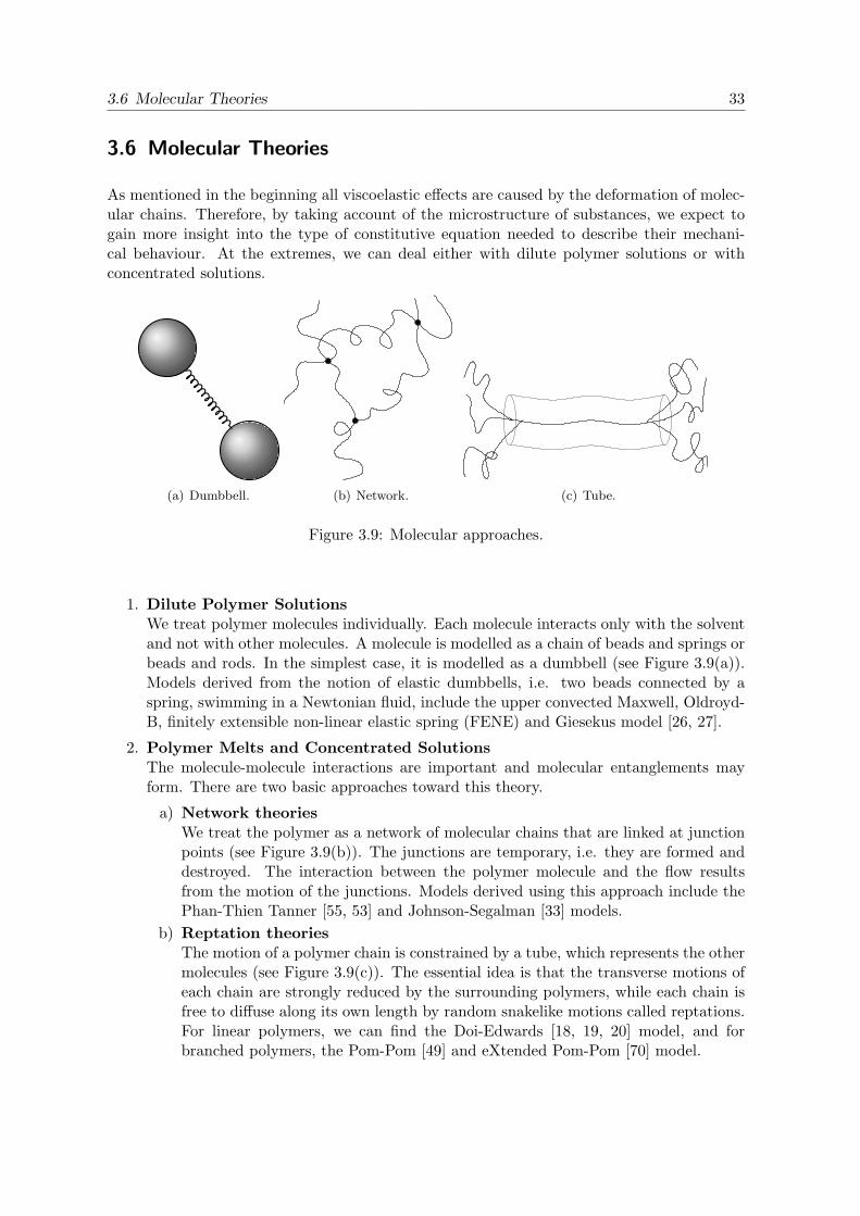
3.6 Molecular Theories 33
3.6 Molecular Theories
As mentioned in the beginning all viscoelastic effects are caused by the deformation of molec-ular chains. Therefore, by taking account of the microstructure of substances, we expect togain more insight into the type of constitutive equation needed to describe their mechani-cal behaviour. At the extremes, we can deal either with dilute polymer solutions or withconcentrated solutions.
(a) Dumbbell. (b) Network. (c) Tube.
Figure 3.9: Molecular approaches.
1. Dilute Polymer SolutionsWe treat polymer molecules individually. Each molecule interacts only with the solventand not with other molecules. A molecule is modelled as a chain of beads and springs orbeads and rods. In the simplest case, it is modelled as a dumbbell (see Figure 3.9(a)).Models derived from the notion of elastic dumbbells, i.e. two beads connected by aspring, swimming in a Newtonian fluid, include the upper convected Maxwell, Oldroyd-B, finitely extensible non-linear elastic spring (FENE) and Giesekus model [26, 27].
2. Polymer Melts and Concentrated SolutionsThe molecule-molecule interactions are important and molecular entanglements mayform. There are two basic approaches toward this theory.
a) Network theoriesWe treat the polymer as a network of molecular chains that are linked at junctionpoints (see Figure 3.9(b)). The junctions are temporary, i.e. they are formed anddestroyed. The interaction between the polymer molecule and the flow resultsfrom the motion of the junctions. Models derived using this approach include thePhan-Thien Tanner [55, 53] and Johnson-Segalman [33] models.
b) Reptation theoriesThe motion of a polymer chain is constrained by a tube, which represents the othermolecules (see Figure 3.9(c)). The essential idea is that the transverse motions ofeach chain are strongly reduced by the surrounding polymers, while each chain isfree to diffuse along its own length by random snakelike motions called reptations.For linear polymers, we can find the Doi-Edwards [18, 19, 20] model, and forbranched polymers, the Pom-Pom [49] and eXtended Pom-Pom [70] model.

34 Chapter 3 Constitutive Equations
In this thesis, the Oldroyd-B model and the Phan-Thien Tanner model are used for thecomputation of viscoelastic fluids. In Section 3.6.1, the Oldroyd-B equations are derived andinvestigated in simple flows. Afterwards, in Section 3.6.2, the Phan-Thien Tanner model isderived and investigated.
3.6.1 Dilute Polymer Solutions
Derivation of the Oldroyd-B Model
We will derive the Oldroyd-B model from a molecular model consisting of a suspension ofHookean dumbbells in a Newtonian solvent. We start with considering an elastic dumbbell,which is thought of as two identical beads connected by a Hookean spring, as shown inFigure 3.10, immersed in a Newtonian solvent, which is treated as a continuum. Each of thetwo beads have mass m and have position vectors r1 and r2 relative to some fixed coordinateframe. Let Q = r2 − r1 denote the end-to-end vector of the dumbbell.
m
m
Q
F(c)1
F(c)2
O
r1
r2
Figure 3.10: Elastic dumbbell.
a. The Equations of Motion for the Beads of the Dumbbell
We can write an equation of motion for each bead of the dumbbell indicating that the massof the bead times its acceleration is equal to the sum of all forces acting on the bead. Inertialforces at the molecular level can be safely neglected. A detailed discussion of the effects ofbead inertia by Schieber and Ottinger [63] shows that bead inertia in polymer models maybe neglected. Additionally, we neglect external forces such as gravity on a bead. Hence, weget the following “force balance” for each bead:
F(f)i + F(c)
i + F(b)i = 0 , i=1,2 (3.56)
consisting of a friction force F(f)i , a connecting spring force F(c)
i and a Brownian force F(b)i .
They will now be described in the foregoing section.

3.6 Molecular Theories 35
1. Friction force F(f)i
This is the force of resistance experienced by a bead as it moves through the so-lution. This friction force is for spherical beads assumed to be given by Stoke’sLaw:
F(f)i = 6πηSa
(dri
dt− u(ri)
)= ζ(dri
dt− u(ri)
). (3.57)
Here, ηS is the solvent viscosity, a is the radius of the bead and u(ri) is the velocity ofthe surrounding fluid at the point with position vector ri. Hence,
(dridt − u(ri)
)is the
velocity of the i-th bead relative to the surrounding fluid. We shall write ζ for 6πηSa.This constant ζ is the so-called friction coefficient.Note that we have neglected any effect which one bead may have on the velocity of thesolvent in the neighbourhood of the other bead. Therefore, our model is restricted toextremely dilute polymer solutions so that the polymer molecules do not see each otherand interact only with the solvent.
2. Spring force F(c)i
The spring connecting the beads exerts a spring force F(c)i on the i-th bead. We
assume this spring force to be given by Hooke’s law:
F(c)1 = −H(r1 − r2) = HQ, (3.58)
F(c)2 = −H(r2 − r1) = −HQ, (3.59)
where H is the spring constant.
3. Brownian forces F(b)i
Brownian forces are the cumulative effect of the exceedingly frequent collisionsbetween a large particle, called a Brownian particle, and the many surrounding muchsmaller fluid particles, which are in incessant thermal motion. The mathematical modelto describe these random movements is the so called Wiener process Wi = Wi(t)(i=1,2), which is a Gaussian stochastic process and is therefore completely characterizedby the mean and autocorrelation of its components Wi,j :
〈Wi,j(t)〉 = 0 ,⟨Wi,j(t)Wi,j(t′)
⟩= min(t′, t). (3.60)
We assume that a bead is large compared to the solvent molecules. This assumptionjustifies the continuum description of the solvent. With the Wiener process we maywrite the Brownian force F(b)
i acting on the i-th bead in the form
F(b)i dt =
√2kTζ dWi, (3.61)
where k is the Boltzmann constant, T is the absolute Temperature and ζ is the frictioncoefficient. The coefficient
√2kTζ may be derived from the principle of equipartition of
energy from kinetic gas theory, which states that in equilibrium
Ekin =12⟨V(t)2
⟩=kT
2, (3.62)

36 Chapter 3 Constitutive Equations
where V(t) is the velocity of the Brownian particle, which is the solution of the stochasticdifferential equation describing the motion of a Brownian particle
mdV(t)dt
= −ζV(t) + F(b)i . (Langevin equation) (3.63)
A detailed derivation may be found in Phan-Thien [54] or Ottinger [78].
Therefore, we obtain the following force balance laws for each bead
−ζ(dr1
dt− u(r1, t)
)+HQ +
√2kTζ
dW1
dt= 0, (3.64)
−ζ(dr2
dt− u(r2, t)
)−HQ +
√2kTζ
dW2
dt= 0. (3.65)
We subtract the two equations from each other. Moreover, we assume that the solvent flowfield is homogeneous so that we may write
u(r2, t) = u(r1, t) + (∇∇∇u)(r2 − r1). (3.66)
If we set W(t) := (W2(t)−W1(t))/√
2 , we obtain the following equation of change for theend-to-end vector of the dumbbell
dQdt
=∇∇∇u ·Q− 2Hζ
Q−
√4kTζdW(t). (3.67)
b. The Fokker-Planck Equation of the dumbbell
The equation (3.67) is a stochastic differential equation and Q(t) is a stochastic process.Methods of stochastic differential equations can be used to convert the stochastic differentialequation (3.67) to the corresponding Fokker-Planck or diffusion equation
∂
∂tp(Q, t) = − ∂
∂Q·[(∇∇∇u ·Q− 2H
ζQ)p(Q, t)− 2kT
ζ
∂
∂Qp(Q, t)
], (3.68)
where p(Q, t) is the probability density function, which characterizes the continuous distri-bution of Q(t). That means that the probability that a dumbbell has an orientation in therange Q to Q+dQ is given by p(Q, t)dQ. Moreover, if g is a function of the connector vectorQ, the expectation of g can be defined as
〈g(Q)〉 =∫g(Q)p(Q, t)dQ. (3.69)
If we multiply the Fokker-Planck equation (3.68) by 〈g(Q)〉, integrate over R3, use the di-vergence theorem and the fact that p approaches zero rapidly enough as Q goes to infinityso that surface integrals can be disregarded, we obtain the equation of change for 〈g(Q)〉

3.6 Molecular Theories 37
as
d
dt〈g(Q)〉 =
⟨(∇∇∇u ·Q)
∂
∂Qg(Q)
⟩+
2kTζ
⟨∂
∂Q· ∂∂Q
g(Q)⟩− 2H
ζ
⟨Q · ∂
∂Qg(Q)
⟩. (3.70)
A similar relation holds for a tensor function g(Q) of any order. We shall be particularlyinterested in the case where g(Q) is the second-order tensor QQ:
∂
∂t〈QQ〉 −∇∇∇u 〈QQ〉 − 〈QQ〉∇∇∇uT =
4kTζ
I− 4Hζ〈QQ〉 . (3.71)
The left hand side of (3.71) is called upper-convected derivative of 〈QQ〉 denoted by∇〈QQ〉
∇〈QQ〉 :=
∂
∂t〈QQ〉 −∇∇∇u 〈QQ〉 − 〈QQ〉∇∇∇uT . (3.72)
Finally we note that, in a system at equilibrium (that is, ∇∇∇u = 0, ddt 〈QQ〉 = 0), Eq. (3.71)gives
〈QQ〉eq =kT
HI. (3.73)
We need these equations to establish expressions for the stress tensor.
c. The Stress Tensor
We follow Bird [7] in this section in deriving the expression for the stress tensor. The totalstress σσσ (as defined in (2.35)) in a polymer solution is presumed to be the sum of a contributionfrom the solvent σσσS and another σσσP , resulting from the presence of the polymer molecules
σσσ = σσσS + σσσP (3.74)= (−pSI + TS) + (−pP + τττ) (3.75)= −pI + T, (3.76)
where p = pS + pP and T = TS + τττ = 2ηSD + τττ ; here ηS is the solvent viscosity,D = 1
2(∇∇∇u +∇∇∇uT ) is the rate-of-deformation tensor. The stress tensor T is zero at equilib-rium. In order to obtain a kinetic theory expression for σσσP , we follow the elementary physicalderivation provided by Kramers [43]. The dumbbell will contribute to the stress in the sus-pension for two principal reasons:
1. Contribution from the Spring Force
An arbitrary plane of area S in the suspension moving with the local solution velocity v mayat any moment be straddled by the two beads of the dumbbell, and there will be a force oftension or compression transmitted through the connector σσσ(c)
P . The orientation of the planeis given by the unit vector n.We want to obtain the average force exerted by all springs of all dumbbells from the left ofthe oriented plane (“ the negative side ”) on the right of that plane (“ the positive side ”).For every dumbbell straddling the plane, this force is given by F(c)
1 if bead “ 1 ” is on the left

38 Chapter 3 Constitutive Equations
1
2
−+
Q
|Q|
n
Plane of area S withunit normal vectorn
Figure 3.11: Spring force.
of the plane (i.e. n ·Q > 0), or F(c)2 if bead “ 2 ” is on the left of the plane (i.e n ·Q < 0).
If we set F(c) = F(c)1 = −F(c)
2 , we obtain the average force exerted by all dumbbells of allorientations for which the connector vector Q intersects the plane in the direction of n as⟨
sgn(n ·Q)F(c)⟩
=∫
over all Qsgn(n ·Q)F(c)p(Q, t) dQ. (3.77)
Now suppose, we have NP elastic dumbbells in the system. The connector vector Q of adumbbell intersects the plane S if and only if either r1 or r2 is contained in the box of volumeS|n ·Q| as shown in Figure 3.11. The probability of finding ri (i=1,2) in this box is given bythe volume of the box divided by the volume of the system V
S|n ·Q|V
.
Since, for the assumed homogeneous system Q(t) and ri(t) are independent random variables,we can first integrate over ri and obtain the average force exerted by all springs through thegiven plane
n · F =[n·nS
∫QF(c)p(Q, t)dQ
], (3.78)
where n = Np/V is the number of dumbbells per unit volume and F is the total averagedforce. This average is to be identified with n · σσσ(c)
P = n · FS . Hence, the contribution of the
dumbbell spring connectors to the stress in the solution is
σσσ(c)P = n
∫QFp(Q, t)dQ = n
⟨QF(c)
⟩= nH 〈QQ〉 . (3.79)

3.6 Molecular Theories 39
2. Contribution from the Bead Motion
The beads themselves may cross an arbitrary plane and bring with them a certain amount of
1
2
−+
(r1 − v)
|r1 − v | ∆t
n
Plane of area Smoving with thefluid velocity v
Figure 3.12: Spring force.
momentum. Now, how many “ 1 ” beads with velocity dr1dt will cross the arbitrary surface S in
time δt? All beads within the volume (dr1dt −v) · δt ·S will cross S in time δt. The probabilitythat r1 is in this box is given by
(dr1dt − v) · δt · SV
. (3.80)
Every bead transports the momentum p = m · (dr1dt − v). The amount of momentum trans-ported across the plane in the normal direction n is then given by
n((dr1
dt− v) · S · n)m(
dr1
dt− v)δt, (3.81)
where n is the number of dumbbells per unit volume and m is the mass of the bead. Ifwe assume that the velocity distribution in a flow system (here consisting of the dumbbellsswimming in the Newtonian solvent) is the same as that in a solution at equilibrium, wecan use the Maxwell-Boltzmann distribution from kinetic gas theory to describe the velocitydistribution of the beads. The Maxwell-Boltzmann distribution is a Gaussian distributiongiven by
〈X〉 = 0, (3.82)⟨X2⟩
=kT
mI, (3.83)

40 Chapter 3 Constitutive Equations
where X is a random variable. Therefore, we get⟨nS · nm(
dr1
dt− v)2δt
⟩= nS · nm
⟨(dr1
dt− v)2
⟩δt = n · nSδtkT I. (3.84)
Hence, the average value of the momentum flux (momentum per unit time per unit area)resulting from beads “ 1 ” of all possible velocities and dumbbells of all possible configurationsis given by
n · n∫kT Ip(Q, t)dQ = n · nkT I
∫p(Q, t)dQ = n · nkT I. (3.85)
We obtain the same result for bead “2”. Since the resulting average value n · 2nkT I must beidentified with n · σσσ(b)
P , we getσσσ
(b)P = 2nkT I. (3.86)
Therefore, the total polymeric stress is given by
σσσP = −pP I + τττ = nH 〈QQ〉+ 2nkT I. (3.87)
The corresponding equation at equilibrium (i.e. τττ = 0) gives us the polymeric contributionto the pressure
pP I = −nH 〈QQ〉eq − 2nkT I(3.73)
= −3nkT I. (3.88)
Finally, we get the Kramers expression for the extra stress tensor
T = TS + τττ = 2ηSD + nH 〈QQ〉 − nkT I. (3.89)
If we use the equation (3.71) in the derivation of the expression for the extra stress tensor,we obtain the Giesekus expression
T = 2ηSD− nζ
4
∇〈QQ〉. (3.90)
We can now eliminate 〈QQ〉 between (3.89) and (3.90) by taking the upper-convected deriva-tive of (3.89) and observing that
∇I = −∇∇∇u− (∇∇∇u)T = −2D, (3.91)
so that
T− 2ηSD = − ζ
4H
[∇T− nkT2D− 2ηS
∇D]. (3.92)
We define the relaxation time λ (time constant for the Hookean elastic dumbbells) and thepolymeric viscosity ηP in terms of the parameters appearing in (3.92) by
λ =ζ
4Hand ηP =
nkTζ
4H= nkTλ. (3.93)

3.6 Molecular Theories 41
With the total viscosity η0 = ηS + ηP , we define the characteristic retardation time for thefluid by
λr =ηSη0λ. (3.94)
Then, equation (3.92) can be written in the form
T + λ∇T = 2η0(D + λ2
∇D), (3.95)
called Oldroyd-B model. By separating out the solvent and polymeric contributions to thestress and substituting the result into (3.95), we obtain the split form of the Oldroyd-Bmodel T = 2ηSD + τττ ,
τττ + λ∇τττ = 2ηPD.
(3.96)
We call τττ the elastic stress tensor. Note that the equations (3.96) reduce to the UCMmodel for ηS = 0.
Behaviour in Simple Flows
For the steady simple shear flow, we obtain similarly to the viscometric functions of the UCMmodel (3.45)
η(γ) =σxyγ
= η0 , N1(γ) = σxx − σyy = 2ληP γ2 , N2(γ) = σyy − σzz = 0 (3.97)
and for the steady uniaxial elongational flow, we obtain
Txx = −2ηS ε+2ηP ε
1− 2λε, Tyy = Tzz = ηS ε−
ηP ε
1 + λε, (3.98)
⇒ ηE(ε) =σxx − σyy
ε= 3ηS + 3
ηP[1− 2λε] [1 + λε]
. (3.99)
Hence, the elongational viscosity still blows up for the Oldroyd-B equations at an elonga-tional rate of 1
2λ . This is caused by the fact that the dumbbells are infinitely extensible andbecome infinitely extended at ε = 1
2λ . This can be seen by taking traces throughout Kramersexpression (3.89), so as to obtain
⟨Q2⟩
=1nH
tr T +3kTH
(3.100)
and using the expressions for Txx, Tyy, T zz (3.98), we see that
⟨Q2⟩
=6ηPλε2
nH (1− 2λε) (1 + λε)+
3kTH
, (3.101)

42 Chapter 3 Constitutive Equations
so that⟨Q2⟩→∞ as ε→ 2λ.
The Oldroyd-B model has been seen to be useful in providing qualitative predictions of theflow of Boger fluids, which have a constant viscosity over a range of shear-rates and a quadraticfirst normal stress difference. Unfortunately, the Oldroyd-B model is unable to adequatelypredict extensional flow behaviour. Nevertheless, it is a good first approach in modellingdilute polymer solutions.
Models with Finite Elongational Viscosity
To overcome the disadvantage of infinitely extensible springs, one might consider derivingmodels with finitely extensible springs. As an alternative to the Hookean spring, Warner [72]proposed the connector force law
F =HQ
1−(Q2/Q2
0
) , (3.102)
for which the spring cannot be extended beyond some finite constant length Q0 andQ2 = tr QQ. Based on this idea the FENE-P [8, 52] and FENE-CR [14] models were derived.Both models predict a finite elongational viscosity at all elongation rates, a non-zero first anda zero second normal stress difference. The FENE-P model shows shear-thinning, the FENE-CR a constant shear viscosity. Giesekus [26, 27] chose the approach to consider anisotropiceffects in the equations of motion for the beads of the dumbbell. He allowed the friction forceand the Brownian motion to be anisotropic and derived an expression for the polymeric partof the extra-stress tensor, which differs only in the addition of a term from the Oldroyd-Bequations (
1 +αλ
ηPτττ
)τττ + λ
δaτττ
δt= 2ηPD, 0 ≤ α ≤ 1, (3.103)
where α is a material parameter, which controls the anisotropy of the fluid. The materialparameter α is obtained for a specific material through fitting of experimental data to theGiesekus model. The Giesekus model predicts shear-thinning, a non-zero first and secondnormal stress difference and a finite elongational viscosity at all elongation rates.

3.6 Molecular Theories 43
3.6.2 Polymer Melts and Concentrated Solutions
Derivation of the PTT Model
In the elastic dumbbell model used in the previous section for the description of dilute poly-mer solutions, polymer-polymer interactions are neglected. However, the range in which thisassumption applies is limited to very small concentrations. Therefore, we take a different ap-proach to model the interactions of the polymer molecules: the network theories of polymericliquids as described by Green and Tobolosky [28], Lodge [45, 46] and Yamamoto [75, 76, 77]. Itwill allow us to describe concentrated polymer solutions and polymer melts. The presentationin this section is based on the books of Bird [7], Tanner [67] and Huilgol and Phan-Thien [30].
Junctions
Segment
(a) Network with temporaryjunctions formed by segments.
1
2 3
N-1N
Q
a
(b) One segment as a freelyjointed bead-rod chain.
Q
(c) Representation of the seg-ments as Hookean springs.
Figure 3.13: The network model.
We imagine a polymeric material as a collection of tangled polymer chains as shown in Fig-ure 3.13. The entangled points, or junctions, are not permanent and are continually beingcreated or destroyed. The chain between two junctions, or segment, is taken to be a freelyjointed, bead-rod chain with end-to-end distance vector Q, i.e. N beads connected by N − 1rigid rods of length a. The statistical treatment of the freely jointed bead-rod chain (fordetails see Bird [7]) shows that the chain can be replaced by a Hookean spring with springconstant
HN =3kT
(N − 1)a2, (3.104)
where k is the Boltzmann constant and T is the absolute temperature. We will suppose thatN is constant for all chains. Eventually, this assumption leads to a single relaxation time.

44 Chapter 3 Constitutive Equations
a. The Equation of Non-Affine Motion for Network Segments
If we assume that the junction points move affinely, it follows that the segment vector Q,which joints two junctions must also move affinely, i.e.
dQdt
= ∇u ·Q. (3.105)
Phan-Thien and Tanner [55, 53], and Johnson and Segalman [33] assumed a non-affine motionof the form
dQdt
= (∇u− ξD) ·Q =: LLL ·Q, (3.106)
where ξ is an arbitrary “slip constant” and LLL := (∇u − ξD) is called effective velocitygradient tensor. The motivation leading to this special form for the effective velocitygradient tensor is based on the notion that the network slips with respect to the effectivemedium, and this slip velocity is an isotropic function of the rate of deformation tensor forthe macroscopically imposed velocity field.
b. Liouville Equation of the Network Segments
Let D(Q, t) be the distribution function of segments, i.e. the number of segments per unitvolume at time t that have an end-to-end vector ranging from Q to Q + dQ is given byD(Q, t)dQ. We have ∫
D(Q, t)dQ = n, (3.107)
where n is the number density of segments, i.e. the number of segments per unit volume.The probability density, which gives the probability that a segment has an end-to-end vectorbetween Q to Q + dQ, is then given by
p(Q, t) =D(Q, t)∫D(Q, t)dQ
=D(Q, t)
n. (3.108)
We can write a balance equation for the distribution function D(Q, t)
d
dtD(Q, t) = (rate of segment creation - rate of segment destruction) . (3.109)
We shall write the rate of segment creation as c, and the rate of segment destruction asβD(Q, t), it being natural to write the destruction rate as being proportional to the numberof segments present. Thus, equation (3.109) can be written as
d
dtD(Q, t) = (c− βD(Q, t)). (3.110)

3.6 Molecular Theories 45
This yields the following Liouville equation
∂D(Q, t)∂t
= − ∂
∂Q·[dQdtD(Q, t)
]+ c− βD(Q, t). (3.111)
We can now define the expectation of a function g of Q by
〈g(Q)〉D =∫g(Q)D(Q, t)dQ. (3.112)
Similar to (3.70) of section 3.6.1, we obtain the following equation of change for dQdt = LLL ·Q
by multiplying (3.111) by QQ and integrating over all configuration space
d
dt〈g(Q)〉D = −
⟨LLL ·Q ∂
∂Q· g(Q)
⟩D
∫c g(Q)dQ− 〈β g(Q)〉D . (3.113)
For g(Q) = QQ, we can deduce
d
dt〈QQ〉D −LLL 〈QQ〉D − 〈QQ〉DLLL
T =∫
(c − β D(Q, t)) QQdQ. (3.114)
c. The Expression for the Stress Tensor
In this section, we use a simple physical argument similar to that given in Section 3.6.1 todeduce the expression for the stress tensor. Initially, let us consider the total Cauchy stresstensor given by
σσσ = σσσS + σσσP = −pI + TS + τττ = −pI + 2ηSD + τττ . (3.115)
To derive the expression for the polymeric contribution to the Cauchy stress, consider anarbitrary plane of area S with outer unit normal vector n as shown in Figure 3.14. Throughthe tension in the segments that pass through the plane, a force is transmitted. To calculatethis force, we first note that the number of segments in the configuration range Q to Q + dQthat intersect the plane is given by
|n ·Q|SD(Q, t)dQ. (3.116)
We obtain the average force exerted by all segments through the plane by
n · F = nS∫
QF(c)N D(Q, t)dQ, (3.117)
where F(c)N is with (3.104) given by
F(c)N = HNQ. (3.118)
This yieldsσσσP =
⟨QF(c)
N
⟩D
= HN 〈QQ〉D . (3.119)

46 Chapter 3 Constitutive Equations
−+
Q
|Q|
n
Plane of area S withunit normal vectorn
Junction
Junction
Segment that cutsthrough plane
Figure 3.14: Physical argument used in calculating the stress tensor σσσP .
We find
d
dtσσσP = HN
d
dt〈QQ〉D
(3.114)=
(3.119)LLLσσσP + σσσPLLLT +HN
(∫cQQdQ− 〈βQQ〉D
). (3.120)
To proceed further, specific forms for c and β must be nominated.
Loss and Creation Rates
First, we note that at equilibrium the creation and loss terms balance one another, so that
ceq = βeqD(Q, t). (3.121)
On this basis, it has been suggested that c may be considered as a function of Q. We takethis Q-dependence of the creation rate to be the same as that for the equilibrium distributionfunction for a freely jointed bead-rod chain. That means, we assume that the distributionfunction for the network segments at the moment of creation is identical to the equilibriumdistribution function for a freely jointed bead-rod chain, which is given by
Dc(Q)eq =(HN
2πkT
)3/2
e−HN2kT
(QQ). (3.122)
Then, we have
〈QQ〉Dc =kT
HNI. (3.123)

3.6 Molecular Theories 47
Now, letc denote the creation rate of all segments independent of Q, then
c(Q) =c ·Dc(Q)eq. (3.124)
Further, Phan-Thien and Tanner [55, 53] assumed that both the creation and loss rates dependon the mean squared segment vector length
⟨Q2⟩D
:
c =c(⟨Q2⟩D
) ·Dc(Q)eq, (3.125)
β = β(⟨Q2⟩D
). (3.126)
To evaluate⟨Q2⟩D
, we note that since σσσP = HN 〈QQ〉D, we must have
⟨Q2⟩D
=1HN
trσσσP =1HN
(trτττ + 3pP ). (3.127)
That means⟨Q2⟩D
is proportional to trτττ . Therefore, we can formulate the creation and loss
rates in terms of trτττ . Next, we assume that the creation ratec(trτττ) is proportional to the
loss rate β(trτττ) withc(trτττ) =
G
kT (1− ξ)β(trτττ), (3.128)
where G is a constant modulus.
Derivation of the Stress Tensor
When we insert our terms for the loss and creation rates in (3.120), we get
d
dtσσσP −LLLσσσP − σσσPLLLT = HN
(c(trτττ)
∫QQDc(Q)eq dQ− β(trτττ) 〈QQ〉D
)= HN
(c(trτττ)
kT
HNI)− β(trτττ)σσσP
(3.128)=
G
(1− ξ)β(trτττ)I− β(trτττ)σσσP .
Hence, we get1
β(trτττ)
(d
dtσσσP −LLLσσσP − σσσPLLLT
)+ σσσP =
G
(1− ξ)I. (3.129)
We can derive the expression for the polymeric contribution to the pressure pP by evaluatingthe expression for the stress tensor σσσPeq = −pP I at equilibrium. With (3.121), we obtain
d
dtσσσP −LLLσσσP − σσσPLLLT = 0. (3.130)
ThenpP I = − G
(1− ξ)I. (3.131)
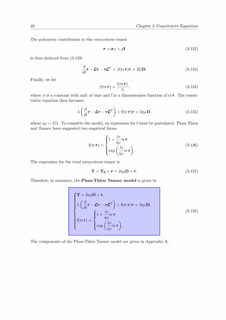
48 Chapter 3 Constitutive Equations
The polymeric contribution to the extra-stress tensor
τττ = σσσP + pI (3.132)
is then deduced from (3.129)
d
dtτττ −LLLτττ − τττLLLT + β(trτττ)τττ = 2GD. (3.133)
Finally, we let
β(trτττ) =f(trτττ)λ
, (3.134)
where λ is a constant with unit of time and f is a dimensionless function of trτττ . The consti-tutive equation then becomes
λ
(d
dtτττ −LLLτττ − τττLLLT
)+ f(trτττ)τττ = 2ηPD, (3.135)
where ηP = Gλ. To complete the model, an expression for f must be postulated. Phan-Thienand Tanner have suggested two empirical forms
f(trτττ) =
1 +
λε
ηPtrτττ
exp(λε
ηPtrτττ).
(3.136)
The expression for the total extra-stress tensor is
T = TS + τττ = 2ηSD + τττ . (3.137)
Therefore, in summary, the Phan-Thien Tanner model is given by
T = 2ηSD + τττ ,
λ
(d
dtτττ −LLLτττ − τττLLLT
)+ f(trτττ)τττ = 2ηPD,
f(trτττ) =
1 +
λε
ηPtrτττ
exp(λε
ηPtrτττ).
(3.138)
The components of the Phan-Thien Tanner model are given in Appendix A.

3.6 Molecular Theories 49
Models Covered by the PTT Equations
PTT
Johnson-Segalman SPTT
Oldroyd-B
UCM Newtonian
ε = 0 ξ = 0
ξ = 0 ε = 0
ηS = 0 λ = 0
Figure 3.15: Models included in the PTT equations.
The PTT model is called exponential PTT (EPTT) model for the choice of
f(trτττ) = exp(λε
ηPtrτττ)
(3.139)
and linear PTT (LPTT) model for
f(trτττ) = 1 +λε
ηPtrτττ . (3.140)
For the choice of ξ = 0, it is called simplified PTT (SPTT) model. Further, the PTTmodel covers the following four kinds of constitutive models (see Figure 3.15): the Johnson-Segalman model (ε = 0), the Oldroyd-B model (ε = 0, ξ = 0), the upper-convected Maxwellmodel (ε = 0, ξ = 0 and η0 = ηP ) and the Newtonian fluid model (λ = 0, ε = 0, ξ = 0 andη0 = ηS).

50 Chapter 3 Constitutive Equations
Behaviour in Simple Flows
For steady shear flow (3.135) becomes
f(trτττ)
τxx τxy 0τxy τyy 00 0 τzz
− λ0 γ 0
0 0 00 0 0
τxx τxy 0τxy τyy 00 0 τzz
+
τxx τxy 0τxy τyy 00 0 τzz
0 0 0γ 0 00 0 0
+ξλ
2
τxx τxy 0τxy τyy 00 0 τzz
0 γ 0γ 0 00 0 0
+
0 γ 0γ 0 00 0 0
τxx τxy 0τxy τyy 00 0 τzz
= ηP
0 γ 0γ 0 00 0 0
.
This leads to the following equations
f(trτττ) τxx − 2λ1γ τxy + λ1ξγ τxy = 0, (3.141)
f(trτττ) τxy − λ1γ τyy + λ1ξγ
2(τxx + τyy) = 0, (3.142)
f(trτττ) τyy + λ1ξγ τxy = 0, (3.143)τzz = 0, (3.144)
from which we obtain the viscometric functions
η(γ) = σxyγ = ηS +f(trτττ) g
2λγ2(1− ξ), (3.145)
N1(γ) = σxx − σyy =2
2(1− ξ)g, (3.146)
N2(γ) = σyy − σzz = − ξ
2(1− ξ)g, (3.147)
where g satisfies (g = τxx + τyy)
(f(trτττ))2g + (λγ)2ξ(2− ξ)g − 2λγ2(1− ξ)ηP = 0. (3.148)
In Figure 3.16, we can see that the PTT fluid and the SPTT (i.e. ξ = 0) fluid are bothshear-thinning. The EPTT model is more shear-thinning than the LPTT model and theshear-thinning effect increases with increasing ε. We use two values of ε, 0.02 and 0.25. Theformer reflects low-density polyethylene (LDPE), while ε = 0.25 is closer to the response ofhigh-density polyethylene melts (HDPE) (Larson [44]). In Figure 3.16(b), we see that theparameter ξ has the strongest influence on shear-thinning.In equation (3.147), we see that for the SPTT model (ξ = 0), we have a zero second normalstress difference. For the Johnson-Segalman and the PTT models, the second normal stressdifference is non-zero and we find the ratio of the normal stress differences to be given by
N1(γ)N2(γ)
= −ξ2. (3.149)
The first and second normal stress differences are plotted for different values at Figure 3.17.To obtain realistic flow behaviour, N1 has to be larger than N2, so that only values of ξbetween 0 and 2 need to be considered. Moreover, experimental data on LDPE and HDPE

3.6 Molecular Theories 51
suggest a value of ξ around 0.1 (Larson [44], Verbeeten [71]).In the case of steady uniaxial elongation (3.135) specializes to
f(trτττ)
τxx 0 00 τyy 00 0 τzz
− λ
ε 0 0
0 − ε2 0
0 0 − ε2
τxx 0 00 τyy 00 0 τzz
+
τxx 0 00 τyy 00 0 τzz
ε 0 00 − ε
2 00 0 − ε
2
+ξλ
2
τxx 0 0
0 τyy 00 0 τzz
ε 0 00 − ε
2 00 0 − ε
2
+
ε 0 00 − ε
2 00 0 − ε
2
τxx 0 00 τyy 00 0 τzz
= ηP
ε 0 00 − ε
2 00 0 − ε
2
,
which has solution
τxx =2ηP ε
f(trτττ)− 2λε(1− ξ), (3.150)
τyy = τzz = − ηP ε
f(trτττ) + λε(1− ξ). (3.151)
Hence, the elongational viscosity is given by
ηE(ε) =σxx − σyy
ε= 3ηS + 3
ηP f(trτττ)[f(trτττ)− 2λε(1− ξ)] [f(trτττ) + λε(1− ξ)]
. (3.152)
For ε = 0, i.e. f(trτττ) = 1, we obtain the Johnson-Segalman model and as shown in Fig-ure 3.18(a) the elongational viscosity becomes infinitely large at an elongation rate of 1
2λ(1−ξ) .Hence, the problem of an infinitely large elongational viscosity is just a little bit shifted in com-parison to the Oldroyd-B model. With ε > 0, this problem is solved. The difference betweenthe exponential form of f(trτττ) and the linear form of f(trτττ) can be seen in Figure 3.18(b).With the linear form, etaE is monotonic in the elongation rate, which approaches a constantat high values of the elongation rate. For the exponential form, etaE goes through a maxi-mum and then decreases at high elongational rates, since the rate of destruction overwhelmsthe rate of creation of network segments. With increasing ε the extensional-thickening effectbecomes stronger.

52 Chapter 3 Constitutive Equations
Shear rate γ
Shea
rvis
cosi
tyη
EPTT ε = 0.02
EPTT ε = 0.25
LPTT ε = 0.02
LPTT ε = 0.25
Oldroyd-B
10−2 100 102 104
1
0.2
0.3
0.4
0.5
0.6
0.7
0.8
0.9
(a) Shear viscosity, SPTT (ξ = 0).
ts
Shear rate γ
Shea
rvis
cosi
tyη
EPTT ε = 0.25, ξ = 0.0
EPTT ε = 0.25, ξ = 0.1
LPTT ε = 0.25, ξ = 0.0
LPTT ε = 0.25, ξ = 0.1
10−2 100 102 104
1
0.2
0.3
0.4
0.5
0.6
0.7
0.8
0.9
(b) Shear viscosity.
Figure 3.16: Shear-thinning.
Shear rate γ
Fir
stnorm
alst
ress
diff
eren
ceN
1
EPTT ε = 0.25, ξ = 0.0
EPTT ε = 0.02, ξ = 0.0
EPTT ε = 0.25, ξ = 0.1
LPTT ε = 0.25, ξ = 0.0
Oldroyd-B
0.2
10−2 100 102 10410−4
10−2
100
102
104
(a) First normal stress difference.
Shear rate γ
Sec
ond
norm
alst
ress
diff
eren
ceN
2 EPTT ε = 0.25, ξ = 0.0
EPTT ε = 0.25, ξ = 0.1
EPTT ε = 0.0, ξ = 0.1
EPTT ε = 0.0, ξ = 0.5
Oldroyd-B
0.4
10−2 100 102 104-0.4
-0.3
-0.2
-0.1
0
0.1
(b) Second normal stress difference.
Figure 3.17: Normal stress differences.
Elongation rate ǫ
Elo
ngationalvis
cosi
tyη
E
Oldroyd-B
EPTT ε = 0.0, ξ = 0.1
0 0.2 0.4 0.6 0.8 1-1000
-500
0
500
1000
(a) Elongational viscosity, Johnson-Segalman,Oldroyd-B.
Elongation rate ǫ
Elo
ngationalvis
cosi
tyη
E
EPTT ε = 0.02
EPTT ε = 0.25
LPTT ε = 0.02
LPTT ε = 0.25
10−2 100 102 10410−1
100
101
102
(b) Elongational viscosity, PTT.
Figure 3.18: Elongational behaviour.

3.7 Summary of Behaviour in Simple Flows 53
3.7 Summary of Behaviour in Simple Flows
To give a short overview over all introduced models in this chapter, Table 3.2 summarizestheir behaviour in simple flows. The symbol means the model predicts the property andthe symbol means the model is not able to predict the property.
Name shear-thinning N1 N2 ηE(ε) finiteContinuum derived
Newtonian
Generalized Newtonian
K-BKZDilute Polymer Solutions
UCM
Oldroyd-B
FENE-P
FENE-CR
GiesekusConcentrated Polymer Solutions
PTT
SPTT
Johnson-Segalman
Doi-Edwards
Pom-Pom
XPPTable 3.2: Overview.
In this thesis, the Oldroyd-B and PTT model are used for numerical computations.


Chapter 4
Mathematical Model
In this chapter, we present the equations, which describe the motion of viscoelastic fluids anddiscuss their non-dimensionalization and the boundary conditions needed in order to solvethem.
4.1 Governing Equations
Let Ω ⊂ R3 be a domain with boundary ∂Ω, filled by an incompressible viscoelastic fluid.Then the mathematical model describing the motion of the viscoelastic fluid consists of threecoupled equations, namely the continuity equation (2.43), the momentum equation (2.47) andthe constitutive equation for the extra-stress tensor given by (3.96) for an Oldroyd-B fluidand by (3.138) for a Phan-Thien Tanner fluid. Here, we will give the system of equations fora Phan-Thien Tanner fluid, because we can obtain the Oldroyd-B model by setting ξ and εto zero. Inserting equation (3.135) into the momentum equation (2.47) yields
ρDuDt
= ρg −∇p+ ηS∆u + div τττ , (4.1)
where g is the body force gravity. Further, we set
β =ηSη0
(4.2)
to obtain a non-dimensional parameter 0 ≤ β ≤ 1 measuring the percentage of the solventNewtonian viscosity to the total viscosity. Therefore, we have ηS = βη0 and ηP = (1− β)η0.Finally, we obtain the following system of equations
ρDuDt
= ρg −∇p+ η0β∆u + div τττ , Momentum Equation
f(trτττ)τττ + λ∇τττ + λξ(τττD + Dτττ) = 2η0(1− β) D, PTT
f(trτττ) =
1 +
λε
(1− β)η0trτττ linear form
exp(
λε
(1− β)η0trτττ), exponential form
div u = 0. Continuity Equation
(4.3)

56 Chapter 4 Mathematical Model
4.2 Non-Dimensionalization
We employ the non-dimensionalization
x∗ =x
L, u∗ =
uU, t∗ =
U
Lt, ρ∗ =
ρ
ρref, p∗ =
1ρrefU2
p, τττ∗ =L
η0Uτττ , g∗ =
g‖ g ‖
,
where L, U , ρref denote the characteristic length, velocity and density scales for the flowrespectively. This leads to the following system of dimensionless equations
Du∗
Dt= −∇p∗ +
1Re
β∆u∗ +1
Rediv τττ∗ +
1Fr2 g∗,
f(trτττ)τττ∗ + Wi∇τττ∗ + Wi ξ(τττ∗D∗ + D∗τττ∗) = 2(1− β) D∗,
f(trτττ) =
1 + Wi ε
(1−β)trτττ∗
exp(
Wi ε(1−β)trτττ∗
),
div u∗ = 0.
(4.4)
We recall the upper convected derivative
∇τττ∗ =
∂τ∗τ∗τ∗
∂t+ u · ∇τ∗∇τ∗∇τ∗ −∇u∗ · τ∗τ∗τ∗ − τττ · ∇u∗T . (4.5)
The dimensionless numbers in (4.4) describe the nature of the flow and are defined as follows:
Definition 4.1 [Dimensionless Numbers]
Re =ULρrefη0
=inertial forcesviscous forces
(4.6)
is the ratio of inertial forces to viscous forces and is called the Reynolds number.
Fr =U√
L ‖ g ‖=
inertial forcesgravitational forces
(4.7)
is the ratio of inertial forces to gravitational forces and is called the Froude number.
Wi = λU
L=λ
T=
relaxation timecharacteristic time
(4.8)
is the ratio of the relaxation time to the characteristic time scale of the fluid process and iscalled the Weissenberg number. It can be regarded as a measure of the elasticity of the fluidin the flow. For high Weissenberg numbers, the fluid behaves like an elastic solid and for lowWeissenberg numbers, it behaves like a Newtonian fluid. Another useful dimensionless numberdescribing the importance of elasticity relative to inertial forces is the so-called elasticitynumber, which we define as
El =WiRe
. (4.9)

4.3 Boundary and Initial Conditions 57
Additionally, we have the non-dimensional material parameters β giving the portion of New-tonian viscosity, ξ the ”slip parameter” and ε describing the elongational behaviour of thefluid. In the following, we will drop the star notation for the sake of simplicity. The completeset of equations is given by components in 3D in Appendix A. We have to solve this system ofequations in the domain Ω during the time interval [0, T ] under adequate boundary and initialconditions. We have ten unknown functions of x ∈ Ω and t ∈ [0, T ], six elastic stress tensorcomponents, the velocity field u = (u, v, w)T and the scalar pressure field p. The system ofpartial differential equations 4.4 is of mixed type and portrays traits of elliptic, parabolic andhyperbolic character [25, 50]. The constitutive equations for the extra stress tensor containthe hyperbolic part, i.e. the components of the extra stress tensor are convected along thestreamlines, while the conservation laws contain the elliptic/ parabolic part.
4.3 Boundary and Initial Conditions
A very detailed discussion on boundary and initial conditions for viscoelastic fluid flows canbe found in Huilgol [30]. We just describe briefly which boundary conditions are used for thesolution of the equations in our computations.
4.3.1 Initial Conditions
For time-dependent flows, a set of initial conditions at time t = 0 is required. We need toprescribe an initial velocity field, i.e.
u(0) = u0. (4.10)
For viscoelastic fluids, a set of initial values for the elastic stress components is also needed.In general, we suppose that the elastic stresses in the fluid are zero at time t = 0, i.e.
τττ(0) = 0. (4.11)
That means, we assume that the elastic stresses are completely relaxed at the beginning.
4.3.2 Solid Boundaries
At walls and obstacles ∂Ω, we assume no-slip boundary conditions for the velocities, i.e.
u = 0, v = 0, w = 0 on ∂Ω. (4.12)
Then, the elastic stresses result from the constitutive equation (see Section 5.2.3).
4.3.3 Inflow and Outflow Boundaries
At the inflow boundary ∂Ωin of the domain, we usually know the velocity field of the flow. Forviscoelastic fluids, the stresses are also required there because they represent the information

58 Chapter 4 Mathematical Model
carried with the fluid from its previous deformation states. Usually, we set Dirichlet boundaryconditions for the velocities at inflow
u = uin on ∂Ωin. (4.13)
We have to be aware that it is not possible to simply prescribe arbitrary stress values atinflow, because they have to be consistent with the constitutive equations. Therefore, weusually assume that the elastic stresses are relaxed at inflow, i.e.
τττ = 0 on ∂Ωin. (4.14)
Renardy [58] showed that, while for the Oldroyd-B model all elastic stress components must beprescribed, for the UCM model prescribing all stress components leads to an over-determinedsystem, which can lead to errors. Resolving this problem is quite difficult in three spacedimensions. A solution to this problem may be found in Renardy [59]. However, we will notuse the UCM model in this thesis.
At the outlet ∂Ωout, the flow is usually well developed and arranged so that a unidirectionalflow results. We assume that the velocity and elastic stress tensor components do not changein the direction of the outward normal vector n of the outflow boundary. That means,we assume homogeneous Neumann boundary conditions for both the velocities and elasticstresses
∂u
∂n=∂v
∂n=∂w
∂n= 0 on ∂Ωout, (4.15)
∂τxx∂n
=∂τyy∂n
=∂τzz∂n
=∂τxy∂n
=∂τxz∂n
=∂τyz∂n
= 0 on ∂Ωout. (4.16)

4.4 The High Weissenberg Number Problem 59
4.4 The High Weissenberg Number Problem
In all published work researchers find that beyond a critical Weissenberg number numericalsimulations fail. This failure is known as the high Weissenberg number problem (HWNP).Although, the critical Weissenberg number is usually frustatingly low. The nonlinearity of thegoverning equations, which becomes increasingly dominant with increasing Weissenberg num-ber, has a strong impact on the performance and stability of numerical methods. Additionally,in view of the nonlinearity of the governing equations, it is not surprising that no completemathematical theory is available on the existence and uniqueness of viscoelastic flows. Thatmeans one might attempt to compute an inexistent or non-unique solution to a problem. Nev-ertheless, it is often the case that critical Weissenberg numbers observed at the discrete levelare numerical artefacts and not a limitation of the model [50]. An attempt to compute aninexistent or non-unique solution would be expected to manifest itself by occurring at a valueWi crit to which one can demonstrate convergence with mesh refinement. However, criticalvalues of the Weissenberg number have often been seen to be mesh dependent. Keunings [39]showed that the attainable Weissenberg number reduces with mesh refinement.One reason why mesh refinement decreases the attainable Weissenberg number is that vis-coelastic models may show loss of evolution. The loss of evolution is an instability in whichshort-wave disturbances sharply increase in amplitude. Joseph and Saut [36] and Joseph etal. [35] showed that viscoelastic models with zero Newtonian viscosity may show loss of evo-lution in time-dependent problems. In general, this instability occurs when certain stressesexceed critical values. Therefore, numerical algorithms may blow up once the Weissenbergnumber reaches a sufficiently large value and the problem will be exacerbated with meshrefinement [40]. This is a severe problem since it is no longer true that convergence of thediscrete solution can be achieved, as the mesh is refined. Joseph and Saut [36] showed thatthe UCM model and models with a Newtonian component do not show this instability. Formodels with a Newtonian component, the elliptic term prevents the onset of the instability.The UCM model cannot show any loss of evolution either, because the positive definitenessof the tensor
τττA = τττ +(1− β)
WiI (4.17)
prevents it. The positive definiteness of the tensor τττA is also an important property for theOldroyd-B model because it prevents the exponential growth of the solution for finite wavenumbers [50]. One might think that by using models with a Newtonian stress componentor the UCM model one might avoid any difficulties with short wave disturbances in timedependent calculations, but numerical errors can cause the loss of evolution at the discretelevel [50]. For example for the UCM and the Oldroyd-B model the positive definiteness of thetensor τττA might be lost at the discrete level in regions of high stress gradients as observedby Dupret et al. [21]. Stabilization techniques introducing a change of variables to enhancethe elliptic character of the momentum equation by making the elliptic operator as large aspossible, such as elastic viscous split stress (EVSS) [51] and adaptive viscoelastic stress split-ting (AVSS) [65], have been shown to improve the numerical stability for steady problems.However, they may pollute the accuracy of transient flow calculations.Transient flow calculations have to cope with additional restrictions on the attainable Weis-senberg number in comparison to steady state algorithms [25]. In a steady state algorithm

60 Chapter 4 Mathematical Model
the systemAx = b (4.18)
can be solved if detA 6= 0, no matter what the eigenvalues of A are. In time dependentsimulations the system
∂x∂t
+ Ax = b (4.19)
has a steady state solution if Re(σ) < 0, in which σ is an eigenvalue of A. For eigenvalueswith Re(σ) ≥ 0 instabilities occur and no steady state solution can be reached. Keiller [38]showed that for the planar Couette flow of an UCM and an Oldroyd-B fluid the requirementRe(σ) < 0 depends on the grid aspect ratio ∆y/∆x. If the wrong aspect ratio is chosen,eigenvalues with Re(σ) ≥ 0 might appear. Keiller showed that this leads to the instabilitycriterion
Wi crit ∼(
∆y∆x
), (4.20)
where ∆x and ∆y are the resolution scales of the computational grid in the streamwise andcross-stream directions respectively. This scaling appears to hold even for complex flows.Smith et al. [66, 64] observed the same dependence of the critical Weissenberg number onthe aspect ratio ∆y/∆x in transient calculations of a flow around a cylinder of an Oldroyd-Bfluid.Renardy [61] pointed out that the difficulty of resolving high-stress gradients, arising nearsolid boundaries and near corner singularities, puts severe limitations on successful numericalsimulations. The cause for the steep stress gradients near solid boundaries is the existence ofboundary layers. The boundary layers occur because of the no-slip condition. The velocityand all its tangential derivatives vanish at the wall, thus making the convected derivativeterms disappear. However, these terms enter the dominant balance in a very short distanceaway from the wall. As a consequence the stress behaviour in a thin layer close to the wallsubstantially differs from the behaviour at a farther distance. This is a transition from vis-cometric behaviour near the boundary to a region where the convected derivative dominates.Renardy showed that the thickness of the boundary layers decreases with increasing Weis-senberg number. For the UCM model the boundary layer thickness is of order Wi−1, for thePTT model, it is of order Wi−1/3, and for the Giesekus model, it is of order Wi−1/2. There-fore, compared to the UCM model, the PTT and the Giesekus model have boundary layersthat sharpen much less rapidly as the Weissenberg number increases. Numerical simulationswith the PTT or Giesekus model are indeed seen to be successful for much higher Weissenbergnumbers than simulations with the UCM model.The numerical solution of viscoelastic flows in domains involving corner singularities is veryproblematic. Because of the hyperbolic nature of the constitutive equations discretizationerrors can be propagated along characteristics, i.e. along the streamlines [50]. Therefore,numerical errors at the corner singularity are propagated downstream. Additionally, Renardy[61] showed that the solution of an UCM fluid in the downstream region of a corner singularitydevelops non-integrable stress singularities. These stress singularities lead to an instability,which causes a stress growth downstream. The source of this instability is a feature of theequations themselves and has nothing to do with the choice of the numerical method. Butthe instability magnifies discretization errors [61]. A downstream growth of errors is alsoobserved for the Oldroyd-B model [24]. For the PTT model, Renardy [60] did not observe adownstream growth of errors. The reason for this might be that the boundary layers in the

4.4 The High Weissenberg Number Problem 61
PTT model have a different scaling and are much wider than in the UCM model. As a result,particles enter the boundary layer and stress relaxation takes over before the downstreaminstability has had a chance to fully manifest itself.Fattal and Kupferman [22, 23] identified a stability criterion on the mesh size ∆x:
∆x ≤ | u |2√−det(∇u)−Wi−1
. (4.21)
This stability condition is very restrictive when convection is weak and in the presence oflarge deformation rates. Therefore, this criterion is easily violated in regions near stagnationpoints and strong deformation rates (e.g. near geometric singularities). Thus, these regions areprone to such a numerical instability. Fattal and Kupferman argued that the stability criterionarises from the fact that the stress experiences a combination of deformation and convection,which gives rise to steep exponential profiles. Even for moderate Weissenberg numbers, thesespatial profiles are poorly approximated by numerical schemes, which are based on polynomialinterpolation. To alleviate the spatial mesh restriction, Fattal and Kupferman proposed areformulation of the constitutive equations. Since the severe restriction on the mesh size isdue to the inadequacy of polynomial interpolation to approximate exponential profiles, theyproposed to make a change of variables into new variables that scale logarithmically withthe stress. However, we cannot just take the logarithm of the stress tensor. In order for thelogarithm of a second-rank tensor to exist, the tensor needs to be positive definite. Therefore,the stress tensor τττ needs to remain strictly positive definite, which cannot be guaranteed.A physical quantity, directly related to the stress, that preserves positive definiteness is theconformation tensor c [31]. The conformation tensor c is a dimensionless measure for thedeformation, which is given by
c =〈QQ〉〈Q2〉eq
, (4.22)
where Q is the end-to-end vector of a polymer chain and 〈·〉 denotes an average over thedistribution space. Hence, Fattal and Kupferman [22, 23] proposed the change of variablesψψψ = log(c) and called the resulting equations the log-conformation representation.Gerritsma [25] noted that for transient viscoelastic calculations the numerical time-step re-quired to obtain bounded solutions decreases rapidly near the limiting Weissenberg number.


Chapter 5
Numerical Method
This chapter deals with the numerical solution of the governing equations. First, we presenta Chorin-type explicit project method. Then, we discuss the time-step restrictions resultingfrom the explicit treatment of the equations. Since the time-step restriction for the diffusiveterms leads to very small time-steps for low Reynolds number flows, we also introduce a semi-implicit projection method. Afterwards, we discuss the spatial discretization on a staggeredgrid and the discrete boundary values.
5.1 Temporal Discretization
5.1.1 Explicit Projection Method
The solution of the equation system (4.4) is not easy to obtain because naive solution ofthe equations leads to a velocity field which is in general not divergence free. To avoidthis problem, we solve the system of equations (4.4) by employing a Chorin-type projectionmethod (Chorin [15], Temam [68]) consisting of the following steps:
Step 1 Solve the constitutive equations for the elastic stresses using the forward Euler method
Wi(τττn+1 − τττn
δt
)= (1− β)2Dn − f(trτττn)τττn −Wi
(u · ∇∇∇τττn −∇∇∇un · τττn − τττn · (∇∇∇uT )n
)−Wi ξ(τττn ·Dn + Dn · τττn).
(5.1)
Step 2 Solve the momentum equations for an intermediate velocity field u∗ ignoring theincompressibility constrained
Re(
u∗ − un
δt
)= β∆∆∆un − Re un · ∇∇∇un +∇∇∇ · τττn +
1Fr2 g. (5.2)
Step 3 Project the intermediate velocity field onto the incompressible velocity field un+1(un+1 − u∗
δt
)= −∇pn+1, (5.3)
∇ · un+1 = 0. (5.4)
64 Chapter 5 Numerical Method
In Step 3, we project the velocity field u∗ onto a divergence free velocity field by taking thedivergence of (5.3) and by enforcing ∇ · un+1 = 0. This leads to a Poisson equation for thepressure
∆pn+1 =(
1δt
)∇ · u∗, (5.5)
which we solve iteratively under adequate boundary conditions by methods like SOR, Red-Black Gauss Seidel or BiCGStab [17]. Finally, the new divergence free velocity field is givenby
un+1 = u∗ − δt∇pn+1. (5.6)
We obtain the boundary condition for the pressure by taking the projection of (5.3) in thedirection of the unit outward normal n to the boundary ∂Ω. This leads to a Neumannboundary condition for the pressure
∂pn+1
∂n= ∇pn+1 · n = − 1
δt
(un+1 − u∗
)· n on ∂Ω. (5.7)
The Neumann problem (5.5) - (5.7) is solvable if the compatibility condition∫Ω∇ · u∗ dV = −
∫∂Ω
(un+1 − u∗
)· n dS (5.8)
is satisfied. Then this solution is unique up to an additive constant. We fix this constant bysetting ∫
Ωpn+1 dV = 0. (5.9)
If the domain Ω is a bounded domain on which velocity boundary conditions are specified,the compatibility condition is satisfied, since∫
∂Ωun+1 · n dS =
∫Ω∇ · un+1 dV = 0. (5.10)
Now, if we set on the boundaryu∗ = un+1 on ∂Ω, (5.11)
we obtain homogeneous Neumann boundary conditions for the pressure
∂pn+1
∂n= −un+1 − u∗
δt· n = 0 on ∂Ω. (5.12)
This method is first-order accurate in time.

5.1 Temporal Discretization 65
5.1.2 Time-Step Control
Since the first-order method (5.1) - (5.4) is explicit, the computational cost per time-step isrelatively low. However, the explicit treatment leads to time-step restrictions for the convec-tive and diffusive terms. These restrictions, ensuring the numerical stability of the method,can be obtained by a stability analysis of the linearized equations. Trebotich et al. [69] findthe restriction of the time step for the convective terms using the Oldroyd-B model for thex-component to be
δtx <∆x
maxi,j,k
[| u | +
√2(τxx + 1−β
We )/Re] , (5.13)
where maxi,j,k[·] denotes the discrete maximum value over all grid cells and | · | denotes theabsolute value of the velocity component. The other components in the y and z-direction areobtained in the same manner, so that the total restriction for the convective terms is givenby
δtc = min [δtx, δty, δtz] . (5.14)
This restriction, known as Courant-Friedrich-Levy (CFL) condition, establishes that convec-tion can take effect only on one further grid cell per time step. We use this restriction inour computations also for the PTT model, because the PTT model generally behaves stablein wider parameter regimes in numerical calculations than the Oldroyd-B model (Alves [3]).Similarly, we restrict the diffusion to act no further than one grid cell per time-step (Wesseling[74])
δtd <
[β
Re
(2
(∆x)2+
2(∆y)2
+2
(∆z)2
)]−1
. (5.15)
Additionally, if gravity acts on the flow (Croce [17]), a further time-step restriction is givenby
δtgx <
maxi,j,k [| u |]∆x
+
√(maxi,j,k [| u |]
∆x
)2
+4 | gx |
∆x
−1
. (5.16)
In the numerical simulation of viscoelastic fluids, we mainly want to investigate flow situations,which are dominated by elastic forces and not by inertial forces, i.e. we want to investigateflows with a high elasticity number El = Wi
Re . Therefore, we usually deal with low Reynoldsnumber flows (Re ≈ 1). In these flows, the time-step restriction for the diffusive terms forcesus to use very small time-steps. To alleviate this restriction, we need to treat the diffusiveterms in the momentum equation implicitly.

66 Chapter 5 Numerical Method
5.1.3 Semi-Implicit Projection Method
Details on the following projection method may be found in Klitz [42]. We use a Crank-Nicolson scheme for the discretization of the diffusive terms
un+1 − un
δt= −∇p+
β
2Re∆∆∆(un+1 + un)︸ ︷︷ ︸
Crank−Nicolson
− (un · ∇∇∇)un +1
Re∇∇∇ · τττn +
1Fr2 g,
and we include the pressure in the equations for the intermediate velocity field by a pressurecorrection scheme based on Bell [4]. The intermediate velocity field u∗ gives a better approx-imation of the actual velocity field un+1, when the pressure term is included in Step 2 of theprojection method. Then, the projection method can be divided into the following steps:
Step 1 Solve the constitutive equations for the elastic stresses using the forward Euler method
τττn+1 = (1− δt
Wif(trτττ))τττn + δt(
2(1− β)Wi
Dn − (un · ∇∇∇)τττn +∇un · τττn + τττn · (∇uT )n)
− δt ξ(τττn ·Dn + Dn · τττn).(5.17)
Step 2 Calculate the intermediate velocity field u∗
(I− δt β
2Re∆∆∆)u∗ = un − δt ·
[(un · ∇∇∇)un +∇pn−
12 − β
2Re∆∆∆un − 1
Re∇∇∇ · τττn +
1Fr2 g
].
(5.18)
Step 3 Solve the Poisson equation for the pressure correction φ and calculate un+1
∆φn+1 = ( 1δt)∇ · u
∗, (5.19)un+1 = u∗ − δt∇φn+1. (5.20)
Step 4 Calculate the new pressure field following Brown [11]
pn+ 12 = pn−
12 + φn+1 − δtβ
2Re∆φn+1. (5.21)
The equation (5.21) is found by a backward substitution of u∗ from equation (5.20) into equa-tion (5.18). The implicit treatment of the diffusive terms leads to three modified Helmholtzequations (5.18), which we solve by an SSOR Preconditioned Conjugate Gradient Method(Klitz [42]). In the explicit projection method, setting u∗|∂Ω = un|∂Ω can be considered asa sufficient approximation of u∗|∂Ω = un+1|∂Ω. However, this approximation is not suffi-cient, when dealing with the Helmholtz equations (I − (δt β/2Re)∆∆∆)u∗ = rhs . Instead, wediscretize the boundary conditions by manipulation of the appropriate entries in the matrix(I− (δt β/2Re)∆∆∆). Therefore, we impose no-slip boundary conditions u∗ = 0 at walls, inflowboundary conditions u∗ = uin and outflow boundary conditions ∇u∗ · n = 0 in the matrixentries as described in detail by Klitz [42].With this method, we can use larger time-steps for low Reynolds number flows and obtainresults much faster than in the explicit case.

5.2 Spatial Discretization 67
5.2 Spatial Discretization
5.2.1 Staggered Grid
τττ i,j,k
pi,j,k
z
x
y
ui+1/2,j,k
vi,j+1/2,k
wi,j,k+1/2
∆xi
∆yj
∆zk
Figure 5.1: Staggered grid
We divide our domain Ω into rectangular subdomains called cells and position our variableson a staggered grid. We position the pressure pi,j,k at the centre of the cells, as well as allsix elastic stress tensor components τττ i,j,k, while we position the velocities ui+1/2,j,k, vi,j+1/2,k,wi,j,k+1/2 at the centre of the cell faces as shown in Figure 5.1. This kind of staggering leadsto a strong coupling between pressure and velocities and therefore prevents spurious modesin the computed pressure known as checkerboard type oscillations. This can be seen in thefollowing way (Gerritsma [25]).
Example 5.1: Consider a square domain Ω in two space dimensions divided into a numberof uniform cells with grid spacing ∆x. The equations we want to solve are
∂u∂t
+∇p = f, (5.22)
∇ · u = 0. (5.23)
The elliptic equation to be solved is then given by
∆p = ∇ · f. (5.24)
Now, suppose we choose all the unknowns at the cell centres. Then, the discretization ofequation (5.22) in the point (see Figure 5.2(a)) identified with (i, j) is given by
un+1i,j − uni,j
δt+pi+1,j − pi−1,j
2∆x= f
(1)i,j , (5.25)
vn+1i,j − vni,j
δt+pi,j+1 − pi,j−1
2∆x= f
(2)i,j . (5.26)

68 Chapter 5 Numerical Method
(a) Pressure points involvedin the discretization of themomentum equation.
(b) Four groups of un-coupled pressure modes(checkerboard).
uvp
(c) Staggered grid.
Figure 5.2: Spurious pressure modes.
It is possible to construct a function p 6= constant which satisfies that the discrete approxima-tion of ∇p, denoted by ∇hp, is zero. We can add such a solution p to p and this change will beinvisible in the momentum equation. Then, the elliptic equation (5.24) has dim(Null(∆)) > 1,which results in a non-uniqueness of the pressure solution. This leads to unwanted oscilla-tions in the discrete pressure solution known as checkerboard oscillations. For example, the“checkerboard” solution p = c1 at , p = c2 at , p = c3 at and p = c4 at , as shownin Figure 5.2(b), satisfies ∇hp = 0. If we choose to position the variables on a staggered gridlike shown in Figure 5.2(c), we have
un+1i+1/2,j − u
ni+1/2,j
δt+pi+1,j − pi,j
∆x= f
(1)i+1/2,j , (5.27)
vn+1i,j+1/2 − v
ni,j+1/2
δt+pi,j+1 − pi,j
∆x= f
(2)i,j+1/2, (5.28)
so that∇hp = 0⇔ p = constant. (5.29)
This leads to a discrete elliptic equation in which all pressure unknowns are connected, andthe occurrence of a pressure checkerboard like in Figure 5.2(b) is avoided. Since the ellipticequation (5.24) due to incompressibility is also present in the computation of viscoelasticfluids, it seems reasonable to locate the velocity and pressure unknowns on a staggered grid.

5.2 Spatial Discretization 69
5.2.2 Discretized Equations
z
x
y
∆xi ∆xi+1
∆xi+1/2
Cell (i, j, k) Cell (i+ 1, j, k)
Figure 5.3: Notation of grid spacing.
We denote the discretization at the position at the cell centre by [·]i,j,k , at the centre of theleft/right cell surface by [·]i±1/2,j,k, at the centre of the bottom/top cell surface by [·]i,j±1/2,k,and at the centre of the front/back cell surface by [·]i,j,k±1/2. Further, we use the notation
∆xi = xi − xi−1 and ∆xi+1/2 = (∆xi + ∆xi+1)/2. (5.30)
We discretize all spatial derivatives using central differences, except for the convective terms,denoted by C(·), in the momentum equations and in the constitutive equations for the elasticstress. Here, the convective terms are approximated by high order schemes such as SMART,VONOS, ENO or WENO. Details of the implementation of these schemes can be found inCroce [17]. We will now give some discretization examples of the for the steps of the explicitprojection method. The discretization formulas for the semi-implicit projection method aredeveloped in the same manner. The xx-component τxx and the xy-component τxy of Step 1of the projection method are approximated by
τxx(n+1)i,j,k =
(1− δt
Wif(trτττ (n)
i,j,k))τxx(n)i,j,k
+ δt
2(1− β)
Wi
[∂u
∂x
](n)
i,j,k
− C(u∂τxx
∂x)(n)i,j,k − C(v
∂τxx
∂y)(n)i,j,k − C(w
∂τxx(n)
∂z)(n)i,j,k
− δt
2(ξ − 1)
[∂u
∂x
](n)
i,j,k
τxx(n)i,j,k +
[(ξ − 2)
[∂u
∂y
](n)
i,j,k
+ ξ
[∂v
∂x
](n)
i,j,k
]τxy(n)i,j,k
− δt
[(ξ − 2)
[∂u
∂z
](n)
i,j,k
+ ξ
[∂w
∂x
](n)
i,j,k
]τxz(n)i,j,k
,
(5.31)

70 Chapter 5 Numerical Method
τxy(n+1)i,j,k =
(1− δt
Wif(trτττ (n)
i,j,k))τxy(n)i,j,k
+ δt
(1− β)
Wi
([∂u
∂y
](n)
i,j,k
+[∂v
∂x
](n)
i,j,k
)− C(u∂τ
xy
∂x)(n)i,j,k − C(v
∂τxy
∂y)(n)i,j,k − C(w
∂τxy
∂z)(n)i,j,k
+ δt
(ξ − 1)
[[∂u
∂x
](n)
i,j,k
+[∂v
∂y
](n)
i,j,k
]τxy(n)i,j,k +
12
[(ξ − 2)
[∂u
∂y
](n)
i,j,k
+ ξ
[∂v
∂x
](n)
i,j,k
]τyy(n)i,j,k
+ δt
12
[(ξ − 2)
[∂u
∂z
](n)
i,j,k
+ ξ
[∂w
∂x
](n)
i,j,k
]τyz(n)i,j,k
+ δt
12
[(ξ − 2)
[∂v
∂x
](n)
i,j,k
+ ξ
[∂u
∂y
](n)
i,j,k
]τxx(n)i,j,k +
12
[(ξ − 2)
[∂v
∂z
](n)
i,j,k
+ ξ
[∂w
∂y
](n)
i,j,k
]τxz(n)i,j,k
,
(5.32)
where e.g. [∂u
∂x
]i,j,k
=ui+1/2,j,k − ui−1/2,j,k
∆xi, (5.33)[
∂u
∂y
]i,j,k
=ui,j+1/2,k − ui,j−1/2,k
∆yi, (5.34)[
∂u
∂z
]i,j,k
=ui,j,k+1/2 − ui,j,k−1/2
∆zi. (5.35)
The terms, which are not defined at the needed cell positions are obtained by linear interpo-lation that is e.g.
ui,j+1/2,k =(∆yjui+1/2,j+1,k + ∆yj+1ui+1/2,j,k)∆xi−1/2
(∆yj + ∆yj+1)(∆xi−1/2 + ∆xi+1/2)
+(∆yjui−1/2,j+1,k + ∆yj+1ui−1/2,j,k)∆xi+1/2
(∆yj + ∆yj+1)(∆xi−1/2 + ∆xi+1/2).
(5.36)
The discretization of the momentum equation for the intermediate velocity field u∗ is givenby
u∗i+1/2,j,k = u(n)i+1/2,j,k + δt
C(∂(u2)
∂x)(n)i+1/2,j,k + C(∂(uv)
∂y)(n)i+1/2,j,k + C(∂(uw)
∂z)(n)i+1/2,j,k
+ δt
1
Reβ
[[∂2u
∂x2
]i+1/2,j,k
+[∂2u
∂y2
](n)
i+1/2,j,k
+[∂2u
∂z2
](n)
i+1/2,j,k
]
+ δt
1
Re
[[∂τxx
∂x
](n)
i+1/2,j,k
+[∂τxy
∂y
](n)
i+1/2,j,k
+[∂τxz
∂z
](n)
i+1/2,j,k
].
(5.37)

5.2 Spatial Discretization 71
Here, the diffusive terms are approximated by[∂2u
∂x2
]i+1/2,j,k
=1
∆xi+1/2
(ui+3/2,j,k − ui+1/2,j,k
∆xi+1−ui+1/2,j,k − ui−1/2,j,k
∆xi
), (5.38)[
∂2u
∂y2
]i+1/2,j,k
=1
∆yj
(ui+1/2,j+1,k − ui+1/2,j,k
∆yj+1/2−ui+1/2,j,k − ui+1/2,j−1,k
∆yj−1/2
). (5.39)
And the terms involving the components of the elastic stress tensor are approximated by[∂τxx
∂x
]i+1/2,j,k
=τxxi+1,j,k − τxxi,j,k
∆xi+1/2, (5.40)
[∂τxy
∂y
]i+1/2,j,k
=τxyi+1/2,j+1/2,k − τ
xyi+1/2,j−1/2,k
∆yi, (5.41)
[∂τxz
∂z
]i+1/2,j,k
=τxyi+1/2,j,k+1/2 − τ
xyi+1/2,j,k−1/2
∆zi, (5.42)
where terms like τxyi+1/2,j+1/2,k are obtained by linear interpolation, i.e.
τxyi+1/2,j+1/2,k =(∆yjτ
xyi,j+1,k + ∆yj+1τ
xyi,j,k)∆xi+1
(∆yj + ∆yj+1)(∆xi + ∆xi+1)
+(∆yjτ
xyi+1,j+1,k + ∆yj+1τ
xyi+1,j,k)∆xi
(∆yj + ∆yj+1)(∆xi + ∆xi+1).
(5.43)
The Laplacian for the pressure in step 3 is discretized at cell centres
[∆p](n+1)i,j,k =
[∂2p
∂x2
](n+1)
i,j,k
+[∂2p
∂y2
](n+1)
i,j,k
+[∂2p
∂z2
](n+1)
i,j,k
=1
∆xi
p(n+1)i+1,j,k − p
(n+1)i,j,k
∆xi+1/2−p
(n+1)i,j,k − p
(n+1)i−1,j,k
∆xi−1/2
+
1∆yi
p(n+1)i,j+1,k − p
(n+1)i,j,k
∆yi+1/2−p
(n+1)i,j,k − p
(n+1)i,j−1,k
∆yi−1/2
+
1∆zi
p(n+1)i,j,k+1 − p
(n+1)i,j,k
∆zi+1/2−p
(n+1)i,j,k − p
(n+1)i,j,k−1
∆zi−1/2
.
(5.44)
The right hand side of the Poisson equation is approximated by[∇ · u∗
δt
]i,j,k
=1δt
([∂u∗
∂x
]i,j,k
+[∂v∗
∂y
]i,j,k
+[∂w∗
∂z
]i,j,k
)
=1δt
(u∗i+1/2,j,k − u
∗i−1/2,j,k
∆xi+v∗i,j+1/2,k − v
∗i,j−1/2,k
∆yi+w∗i,j,k+1/2 − w
∗i,j,k−1/2
∆zi
).
(5.45)
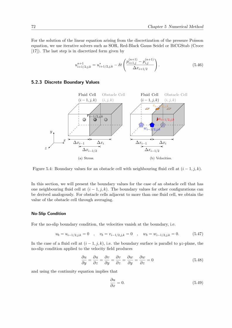
72 Chapter 5 Numerical Method
For the solution of the linear equation arising from the discretization of the pressure Poissonequation, we use iterative solvers such as SOR, Red-Black Gauss Seidel or BiCGStab (Croce[17]). The last step is in discretized form given by
un+1i+1/2,j,k = u∗i+1/2,j,k − δt
(p
(n+1)i+1,j − p
(n+1)i,j
∆xi+1/2
). (5.46)
5.2.3 Discrete Boundary Values
z
x
y
∆xi−1 ∆xi
∆xi−1/2
Fluid Cell(i− 1, j, k)
Obstacle Cell(i, j, k)
τττ i−1/2,j,k
(a) Stress.
ui−1/2,j,k
vi−1/2,j,k
wi−1/2,j,k
∆xi−1 ∆xi
∆xi−1/2
Fluid Cell(i− 1, j, k)
Obstacle Cell(i, j, k)
(b) Velocities.
Figure 5.4: Boundary values for an obstacle cell with neighbouring fluid cell at (i− 1, j, k).
In this section, we will present the boundary values for the case of an obstacle cell that hasone neighbouring fluid cell at (i − 1, j, k). The boundary values for other configurations canbe derived analogously. For obstacle cells adjacent to more than one fluid cell, we obtain thevalue of the obstacle cell through averaging.
No-Slip Condition
For the no-slip boundary condition, the velocities vanish at the boundary, i.e.
ub = ui−1/2,j,k = 0 , vb = vi−1/2,j,k = 0 , wb = wi−1/2,j,k = 0. (5.47)
In the case of a fluid cell at (i− 1, j, k), i.e. the boundary surface is parallel to yz-plane, theno-slip condition applied to the velocity field produces
∂u
∂y=∂u
∂z=∂v
∂y=∂v
∂z=∂w
∂y=∂w
∂z= 0 (5.48)
and using the continuity equation implies that
∂u
∂x= 0. (5.49)

5.2 Spatial Discretization 73
Thus, only the terms ∂v∂x and ∂w
∂x are non-zero. Before we can calculate the elastic stresses atthe boundary, we have to evaluate their values at the boundary by linear interpolation
τττ b = τττ i−1/2,j,k =∆xiτττ i−1,j+1,k + ∆xi−1τττ i,j,k
∆xi + ∆xi−1. (5.50)
Because of the no-slip boundary condition the constitutive equations for the elastic stressesspecialize to
τxx(n+1)i−1/2,j,k =
(1− δt
Wif(trτττ (n)
i−1/2,j,k))τxx(n)i−1/2,j,k
− δt
ξ
[∂v
∂x
](n)
i−1/2,j,k
τxy(n)i−1/2,j,k + ξ
[∂w
∂x
](n)
i−1/2,j,k
τxz(n)i−1/2,j,k
,
τyy(n+1)i−1/2,j,k =
(1− δt
Wif(trτττ (n)
i−1/2,j,k))τyy(n)i−1/2,j,k − δt(ξ − 2)
[∂v
∂x
](n)
i−1/2,j,k
τxy(n)i−1/2,j,k,
τzz(n+1)i−1/2,j,k =
(1− δt
Wif(trτττ (n)
i−1/2,j,k))τzz(n)i−1/2,j,k − δt(ξ − 2)
[∂w
∂x
](n)
i−1/2,j,k
τxz(n)i−1/2,j,k,
τxy(n+1)i−1/2,j,k =
(1− δt
Wif(trτττ (n)
i−1/2,j,k))τxy(n)i−1/2,j,k
− δt
ξ
2
[∂v
∂x
](n)
i−1/2,j,k
τyy(n)i−1/2,j,k +
ξ
2
[∂w
∂x
]τyz(n)i−1/2,j,k
− δt
(ξ − 2)
2
[∂v
∂x
](n)
i−1/2,j,k
τxx(n)i−1/2,j,k +
(1− β)Wi
[∂v
∂x
](n)
i−1/2,j,k
,
τxz(n+1)i−1/2,j,k =
(1− δt
Wif(trτττ (n)
i−1/2,j,k))τxz(n)i−1/2,j,k
− δt
ξ
2
[∂v
∂x
](n)
i−1/2,j,k
τyz(n)i−1/2,j,k +
ξ
2
[∂w
∂x
]τzz(n)i−1/2,j,k
− δt
(ξ − 2)
2
[∂w
∂x
](n)
i−1/2,j,k
τxx(n)i−1/2,j,k +
(1− β)Wi
[∂w
∂x
](n)
i−1/2,j,k
,
τyz(n+1)i−1/2,j,k =
(1− δt
Wif(trτττ (n)
i−1/2,j,k))τyz(n)i−1/2,j,k
− δt
(ξ − 2)
2
[∂v
∂x
](n)
i−1/2,j,k
τxz(n)i−1/2,j,k +
(ξ − 2)2
[∂w
∂x
](n)
i−1/2,j,k
τxy(n)i−1/2,j,k
,
(5.51)
where [∂v
∂x
]i−1/2,j,k
=vi,j,k − vi−1,j,k
∆xi−1/2and
[∂w
∂x
]i−1/2,j,k
wi,j,k − wi−1,j,k
∆xi−1/2, (5.52)

74 Chapter 5 Numerical Method
with
vi,j,k =∆yj−1/2vi,j+1/2,k + ∆yj+1/2vi,j−1/2,k
∆yj−1/2 + ∆yj+1/2, (5.53)
vi−1,j,k =∆yj−1/2vi−1,j+1/2,k + ∆yj+1/2vi−1,j−1/2,k
∆yj−1/2 + ∆yj+1/2, (5.54)
wi,j,k =∆zk−1/2wi,j,k+1/2 + ∆zk+1/2wi,j,k−1/2
∆zk−1/2 + ∆zk+1/2, (5.55)
wi−1,j,k =∆zk−1/2wi−1,j,k+1/2 + ∆zk+1/2wi−1,j,k−1/2
∆zk−1/2 + ∆zk+1/2. (5.56)
Finally, we obtain our values τττ (n+1)i,j,k by linear extrapolation, i.e.
τττ(n+1)i,j,k =
∆xi + ∆xi−1
∆xi−1τττ
(n+1)i−1/2,j,k −
∆xi∆xi−1
τττ(n+1)i−1,j,k. (5.57)
The velocity components, which are lying directly on the boundary, can be set to zero. Thus,in our example (see Figure 5.4), we have
ub = ui−1/2,j,k = 0. (5.58)
For the velocity components, which have no direct value on the boundary, the zero boundaryvalue is enforced by linear extrapolation
vi,j+1/2,k = − ∆xi∆xi−1
vi−1,j+1/2,k and wi,j,k+1/2 = − ∆xi∆xi−1
wi−1,j,k+1/2. (5.59)
Inflow Conditions
At inflow, we assume the elastic stresses to be zero. The boundary values for the stresses arethen obtained by linear extrapolation as
τττ i−1/2,j,k = − ∆xi∆xi−1
τττ i−1,j,k. (5.60)
The velocities are explicitly given at the inflow boundary. Let us denote the prescribed valuesas uin = (uin, vin, win). The Dirichlet condition u = uin can be directly set for the velocitycomponent situated at the boundary face and is obtained by linear extrapolation for thevelocity values, which have no direct value on the boundary. Thus, we set
ui−1/2,j,k = uin, (5.61)
vi,j+1/2,k =∆xi + ∆xi−1
∆xi−1vin −
∆xi∆xi−1
vi−1,j+1/2,k, (5.62)
wi,j,k+1/2 =∆xi + ∆xi−1
∆xi−1win −
∆xi∆xi−1
wi−1,j+1/2,k. (5.63)

5.2 Spatial Discretization 75
Outflow Conditions
We assume homogeneous Neumann boundary conditions at the outlet for both stresses andvelocities. That means, we have
∂τττ i−1/2,j,k
∂n= (1, 0, 0)T · ∇τττ i−1/2,j,k =
∂τττ i−1/2,j,k
∂x=τττ i,j,k − τττ i−1,j,k
∆xi−1/2= 0. (5.64)
Therefore, we set
τττ i,j,k = τττ i−1,j,k, (5.65)ui−1/2,j,k = ui−3/2,j,k , vi,j+1/2,k = vi−1,j+1/2,k , wi,j,k+1/2 = wi−1,j,k+1/2. (5.66)
Periodic Boundary Conditions
only semi-implicit
uvp, τττ
Figure 5.5: 2D periodic boundary conditions in x-direction.
Periodic boundary conditions are a set of boundary conditions used to simulate an infinitelylarge domain in the periodic directions. When a periodic boundary condition is set in onedirection, we can use it to simulate two dimensions (e.g. x and y), while leaving the thirddirection (z) open and obtain pseudo 2D simulations. We glue the domain at the boundarytogether by exchanging the values at the boundary of the domain as shown in Figure 5.5.That means the velocity values u ( ) and v ( ), the elastic stresses and the pressure ( )are exchanged, so that the domain boundaries overlap by one cell in the periodic direction.In the semi-implicit projection method the velocity components at the boundary have to beexchanged before and after the solution of the Helmholtz system (see Figure 5.5), in additionto the exchange of the two velocity values in the explicit case (Klitz [42]).

76 Chapter 5 Numerical Method
5.3 Algorithm
Finally, we obtain the following algorithms to compute transient viscoelastic flows.
Algorithm 5.3.1: Explicit Comp. of Viscoelastic Flows(u, p, τττ)Set t = 0, n = 0.Assign initial values to u, p, τττ .
while t ≤ tend
do
Select δt according to (5.13)-(5.16).Set boundary values for u, p.Set boundary values for τττ .Compute τττ (n+1) according to (5.1).Update boundary values for τττ .Set boundary conditions for u∗.Compute u∗ according to (5.2).Compute the right-hand side of the pressure Poisson equation (5.5).Solve the pressure Poisson equation (5.5).Compute u(n+1) according to (5.6).t = t+ δt, n = n+ 1.
Algorithm 5.3.2: Semi Implicit Comp. of Viscoelastic Flows(u, p, τττ)Set boundary values for the ∆ part of Helmholtz matrix.Set t = 0, n = 0.Assign initial values to u, p, τττ .
while t ≤ tend
do
Select δt.Set boundary values for u, p.Set boundary values for τττ .Compute τττ (n+1) according to (5.17)Update boundary values for τττ .Compute the right-hand side of the Helmholtz equation (5.18).Set boundary conditions for u∗.Solve the Helmholtz system for u∗ according to (5.18).Compute the right-hand side of the Poisson equation (5.19).Solve the Poisson equation (5.19) for the pressure difference φ(n+1)
Compute u(n+1) according to (5.20).Compute p(n+1/2) according to (5.21).t = t+ δt, n = n+ 1.
The semi-implicit approach is useful for the computation of low Reynolds number flows(Re ≈ 1) and the explicit method is useful for the computation of flows with higher Reynoldsnumbers (Re ≈ 100).

Chapter 6
Parallelization
To compute transient viscoelastic flows, we need to solve the governing equations for tenunknowns at each time-step. This is a huge computational task especially for complex flowsituations. Results are only achievable within a decent time by increasing the computationalefficiency. This can be done by parallelization, where the computational work and the memoryrequirements are divided between several processors. The processors communicate with eachother and so cooperate on the solution to a problem. NaSt3DGP [1] is already fully parallelizedbased on a domain decomposition approach (Griebel [29]). In this chapter, we will describethis approach shortly.
6.1 Domain Decomposition and Communication
Ω1
Ω2 Ω3
Ω4
(a) Overlapping subdomains.
Ω1 Ω4
u v p,τττu (only semi-implicit)
(b) Exchange of values.
Figure 6.1: Domain decomposition and communication.

78 Chapter 6 Parallelization
We decompose our domain Ω into subdomains Ω1 . . .ΩN . Each process treats one subdomainand computes the unknowns belonging to this domain. Therefore, a process does not requireaccess to the entire data structure. Hence, the solution of iterative algorithms can be dividedamong the processes.The processes interact with one another by exchanging values on an artificial boundary. Thisensures the convergence of the parallelized algorithm and that the processes do not try to useuninitialized values in their computation. Depending on the discretization stencil, we needone or more cell rows wrapped around the domain (Croce [17]), e.g. we need two artificialcell rows for the VONOS scheme and three for the WENO scheme. The enlargement by thisartificial boundary of the subdomains leads to an overlapping of the domains as shown inFigure 6.1(a). The velocity, pressure and stress tensor values exchanged at each time step areshown in Figure 6.1(b) for the example of two neighbouring processes in a two dimensionaldomain with one cell row as artificial boundary. For a process surrounded by other processes,the boundary strip values are shown in Figure 6.2. To ensure up to date corner values, wehave to communicate the corner values two times in 2D and three times in 3D. In additionto the communication of the velocity, pressure and stress values at each time-step, we haveto communicate the pressure values at each iteration of the Poisson solver, and if we use thesemi-implicit projection method (see Section 5.1.3), the velocity values at each iteration ofthe Helmholtz solver. Furthermore, in the case of the semi-implicit projection method, theHelmholtz solver requires the communication of the velocity values at the boundary of theprocess domain denoted by in Figure 6.1(b) (Klitz [42]).We have to be aware that the computation is slowed down by the time these communicationstake and by the idling time, when processes are waiting to obtain necessary values. Weobtain the optimal speedup if the amount of interprocessor communication is minimized andthe calculated load is evenly balanced. In general, we can achieve a balanced computingload by the decomposition of the domain into subdomains of nearly equal size, so that eachprocessor treats approximately the same number of unknowns.
(a) Subdomains.
u
vp, τττ
(b) Values in the domain and artificial boundarystrip.
Figure 6.2: Artificial boundary strip.

6.2 Measuring Performance 79
6.2 Measuring Performance
For the communication between processes, we use MPICH [2], which is a freely available,portable implementation of the library specification for message-passing MPI (Message Pass-ing Interface). MPICH consists of a set of routines callable from Fortran, C, or C++ andother programming languages. The“CH”in MPICH stands for“Chameleon,” symbol of adapt-ability to one’s environment and thus of portability. MPI’s portability enables it to exploitnative hardware features to optimize performance and there is no need to modify your sourcecode when you port your application to a different platform that supports the MPI standard.Additionally, MPI has a high functionality with over 115 routines.The numerical results shown in this thesis were computed on the parallel computer Himalayaof the Institute for Numerical Simulation and the Sonderforschungsbereich 611. The High-Performance Cluster Computer Himalaya consists of 128 nodes, which are connected by aMyrinet infrastructure. This infrastructure allows fast communication between the nodesseparated from the service ethernet and without the TCP/IP protocol overhead. Each nodecontains two Intel Xeon EM 64 T 3.2 GHz CPUs and 4-6 GB memory. Himalaya has a peakperformance of 1638.4 GFlop/s.As mentioned above, the reduction of the execution time for a parallel algorithm is limitedby the cost of communications and the idling time of the processors. We want to measure thegain in computation speed for the parallel algorithm and therefore we define:
Definition 6.1 [Speed-up, efficiency]Let p be the number of processors and T (p) the execution time of the parallel algorithm usingp processors. Then, the speed-up of a parallel algorithm is given by
S(p) =T (1)T (p)
=execution time serial algorithm
execution time using p processors. (6.1)
The efficiency is defined by
E(p) =T (1)p · T (p)
=S(p)p
=speed-up
number of processors. (6.2)
We measure the speed-up and efficiency of our parallized code in a fixed geometry which isthen divided among an increasing number of processors. As example, we consider the planechannel flow through a channel of length 10 and height 1 in a domain Ω = 10× 1× 1. In thethird direction, we employ periodic boundary conditions. We set the parabolic steady statesolution for the velocity and the steady state solution for the stress components at the inflowboundary (see Section 7.1.1). At the outflow boundary, we set the steady state solution forthe velocity and homogeneous Neumann boundary condition for the stress components. Weresolve the channel with 400× 40× 40 grid cells. We use the semi-implicit projection methodto perform the computations for the Oldroyd-B model with Wi = 0.5, Re = 1 and β = 0.1.We perform the computations until the time t = 0.01, which takes the semi-implicit solver96 time-steps. We solve the pressure Poisson equation by a Jacobi preconditioned BiCGStabmethod and the Helmholtz equation for the intermediate velocity by a Jacobi preconditionedCG method.
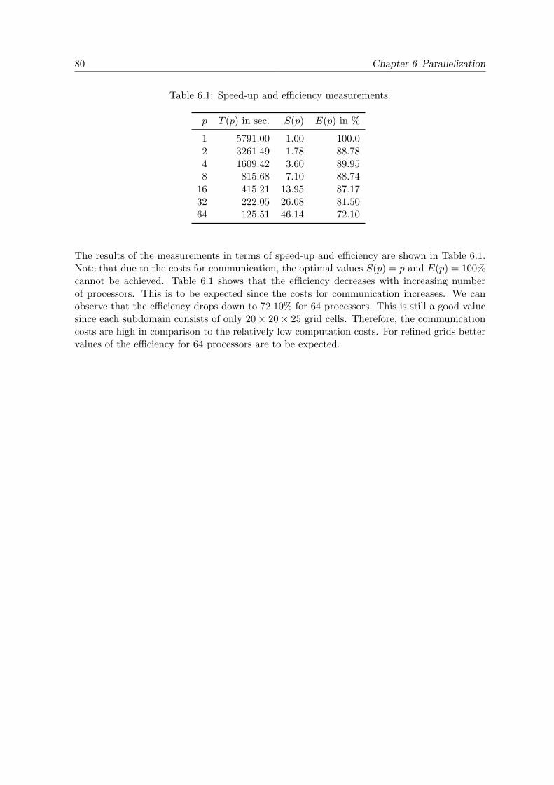
80 Chapter 6 Parallelization
Table 6.1: Speed-up and efficiency measurements.
p T (p) in sec. S(p) E(p) in %
1 5791.00 1.00 100.02 3261.49 1.78 88.784 1609.42 3.60 89.958 815.68 7.10 88.74
16 415.21 13.95 87.1732 222.05 26.08 81.5064 125.51 46.14 72.10
The results of the measurements in terms of speed-up and efficiency are shown in Table 6.1.Note that due to the costs for communication, the optimal values S(p) = p and E(p) = 100%cannot be achieved. Table 6.1 shows that the efficiency decreases with increasing numberof processors. This is to be expected since the costs for communication increases. We canobserve that the efficiency drops down to 72.10% for 64 processors. This is still a good valuesince each subdomain consists of only 20× 20× 25 grid cells. Therefore, the communicationcosts are high in comparison to the relatively low computation costs. For refined grids bettervalues of the efficiency for 64 processors are to be expected.
Chapter 7
Numerical Results
This chapter contains our numerical results. We validate our implementations by the investi-gation of the numerical approximation of the analytical solution for transient plane Poiseuilleflow of an Oldroyd-B fluid and by a convergence study of a three-dimensional gravity drivenflow through an infinite rectangular channel. Furthermore, we examine the flow through athree-dimensional rectangular channel, the flow over a hole and the Karman vortex streetbehind an inclined plate and investigate the results for the different models. Since we want tocompare the models in terms of their stress predictions, we need suitable methods to visualizethe stress tensor.
Visualization of the Stress Tensor
The interpretation and visualization of the stress state of a fluid is a difficult task. Eventhough, the plotting of all six components of the stress tensor gives some information aboutthe behaviour of the stress model equations, it is unclear how to relate these values to thetotal stress state of the fluid at a given point. In solid materials the determination of maxi-mum normal stresses and shear stresses at a point is of considerable interest in the design ofstructures because failures occur when the magnitudes of stresses exceed allowable (normalor shear) stress values. These maximum stresses are given by the eigenvalues of the Cauchystress tensor and are called principal stresses. However, for a fluid the flow dependent shearand normal stresses are of greater interest than the maximum stresses since the propertiesof a fluid material like the shear-dependent viscosity, elongational viscosity or normal stressdifferences, depend on the flow directed shear and normal stresses. We follow the approachof Bollada and Phillips [10] in defining a flow dependent shear and normal stress measure.First, we substract the mean normal stress
σm =13
trσσσ (7.1)
from the Cauchy stress tensor to obtain the traceless deviatoric stress tensor
σdσdσd = σσσ − σmI. (7.2)
Note that the mean normal stress σm can be interpreted as the pressure. This approach leadsfor the Oldroyd-B and PTT model to the equation
σdσdσd = σσσ − σmI = −pI + 2βD + τττ − 13
(−3p+ div u + trτττ) I = 2ηD + τττ − 13
trτττ . (7.3)
82 Chapter 7 Numerical Results
Furthermore, we consider the direction of the flow field
u =u‖ u ‖
(7.4)
and choose two arbitrary directions, u1⊥, u2
⊥ satisfying
u1⊥ · u = u2
⊥ · u = u1⊥ · u2
⊥ = 0 (7.5)
with ‖ u1⊥ ‖=‖ u2
⊥ ‖= 1 to define a positive flow dependent shear stress measure S1, inde-pendent of the choice of u1
⊥ and u2⊥, as
S1 =√(
u · σdσdσd · u1⊥)2 +
(u · σdσdσd · u2
⊥)2 (7.6)
and a flow dependent normal stress measure S2 in direction of the streamlines as
S2 = u · σdσdσd · u. (7.7)
Then, we define the principal stress as
pS =√S2
1 + S22 . (7.8)
We use these stress measures to visualize the stress tensor with ParaView[32] and Matlab.

7.1 Unsteady Poiseuille Flow of an Oldroyd-B Fluid 83
7.1 Unsteady Poiseuille Flow of an Oldroyd-B Fluid
The unsteady Poiseuille Flow of an Oldroyd-B Fluid in a plane channel is a benchmarkproblem for viscoelastic computations since an analytical solution exists for both the steadyand the transient problem. In this section, we want to determine the quality of our numericalsolution by comparison with the analytical solution for both the steady and the transientproblem. Therefore, we first present the analytical solution. Then, we compare the transientdevelopment of our numerical solution against the analytical solution at predetermined pointsin the flow domain. And last, we examine the convergence of the numerical solution to theanalytical steady state solution with mesh refinement. We find a very good agreement betweenthe transient analytical solution and the numerical solution and we observe that the numericalsolution converges quadratically to the steady state analytical solution.
7.1.1 Analytical Solution
We present the analytical solution of the Poiseuille flow of an Oldroyd-B fluid for both thevelocity and stress components. The Poiseuille flow is the flow of a fluid through a channeldriven by a constant pressure gradient. For the mathematical description of this problem intwo space dimensions, let us consider the constant pressure gradient
∂p
∂x= κ. (7.9)
Now, we assume a velocity distribution of the form
(u(y, t), 0, 0) with 0 < y < L and t > 0 (7.10)
with boundary conditionsu(0, t) = 0 and u(L, t) = 0 (7.11)
and initial conditionu(y, 0) = 0 with 0 < y < L. (7.12)
Then, the equation of continuity is automatically satisfied, and the flow of the fluid is givenby the equation of motion
ρ∂u
∂t= −κ+∇ ·T, (7.13)
where T is given by the Oldroyd-B equations (3.95). Waters and King [73] derived the solutionfor this problem and non-dimensionalized the solution in the following manner
y∗ =y
L, u∗ =
u
U, U = −κL
2
8η0, t∗ =
η0t
ρL2. (7.14)
This leads to the dimensionless numbers
El =λη0
ρL2=
WiRe
, β =ηSη0, Wi = λ
U
L, Re =
ULρ
η0. (7.15)

84 Chapter 7 Numerical Results
The solution of Waters and King [73] is given by
u∗(y∗, t∗) = 4y∗(1− y∗)− 32∞∑n=1
sin(Ny∗)N3
GN (El, t∗), (7.16)
where
GN (El, t∗) = exp(−αN t
∗
2El
)[cosh
(βN t
∗
2El
)+γNβN
sinh(βN t
∗
2El
)](7.17)
and
N = (2n− 1)π, αN = 1 + ElN2, (7.18)
β2N = α2
N − 4N2El, βN =√β2N , (7.19)
γN = 1 +N2El(β − 2). (7.20)
If β2N < 0, then GN (El, t∗) changes to
GN (El, t∗) = exp(−αN t
∗
2El
)[cos(βN t
∗
2El
)+γNβN
sin(βN t
∗
2El
)](7.21)
withβN =
√−β2
N . (7.22)
The corresponding Newtonian solution is given by
u∗(y∗, t∗) = 4y∗(1− y∗)− 32∞∑n=1
sin(Ny∗)N3
exp(−N2t∗
). (7.23)
Note that we have to fit our non-dimensional time scale (t∗our = (U/L)t) to the time scale ofthe analytic solution (t∗ana = (η0t)/(ρL2))
t∗ana =η0t
ρL2= El
t
λ= El
t U
Wi L=t∗ourRe
. (7.24)
The Newtonian and the Oldroyd-B fluid have the same steady state solution (t→∞) for thevelocity
A(y) = u∗(y∗) = 4y∗(1− y∗). (7.25)
In the following, we will drop the star notation for the sake of simplicity. The steady statesolution for the stress components of the Oldroyd-B fluid is given by
τxx = 2 Wi∂u
∂yτxy = 2 Wi (1− β)
(∂u
∂y
)2
= 2 Wi (1− β)A′(y)2, (7.26)
τxy = (1− β)∂u
∂y= (1− β)A′(y), (7.27)
τyy = 0, (7.28)

7.1 Unsteady Poiseuille Flow of an Oldroyd-B Fluid 85
whereA′(y) =
dA(y)dy
. (7.29)
Carew et al. [13] found the analytical expressions for the stress components using the solutionof Waters and King to be
τyy = 0, (7.30)
τxy =(1− β)
El
[ElA′(y)− 32
∞∑n=1
cos(Ny)N2
HN (El, t)
]+ Cxy(El, y) exp
(− t
El
), (7.31)
τxx = 2ReCxy(El, y)
[A′(y) exp
(− t
El
)t− 32
∞∑n=1
cos(Ny)N2
IN (El, t)
]
+ 2Re (1− β)A′(y)
[A′(y)El− 32
∞∑n=1
cos(Ny)N2
HN (El, t)
]
− 64 ReA′(y)(1− β)El
∞∑n=1
cos(Ny)N2
JN (El, t)
+2 · 322 Re (1− β)
El
∞∑n,m=1
cos(Ny)N2
cos(My)M2
KNM (El, t) + Cxx(El, y) exp(− t
El
),
(7.32)
where M = (2m − 1)π, and Cxy and Cxx are time-independent functions defined by the re-quirement that τxy and τxx are zero at time t = 0, respectively. The coefficients HN (El, t),IN (El, t), JN (El, t) and KNM (El, t) are given in Appendix B as well as details on their deriva-tion.

86 Chapter 7 Numerical Results
7.1.2 Numerical Approximation
In this section, we investigate the quality of the numerical solution. Therefore, we consider achannel of length 8.0 (x-direction) and height 1.0 (y-direction), as illustrated in Figure 7.1.Furthermore, we choose a channel width of 1.0 (z-direction), but we impose periodic boundaryconditions in the z-direction, so that we obtain a pseudo-2D simulation. The Reynolds number
8.0
1.0 12
3
5.0u = uana
τxx = τxx(ana)
τxy = τxy(ana)
u = uana∂τik∂n
= 0
Figure 7.1: Setup of the channel for the Poiseuille flow problem.
is set to 1.0 and β is taken to be 0.1, i.e. the solvent Newtonian contribution to the totalviscosity is only 10%. We compute the solution with the semi-implicit scheme and use theVONOS-scheme for the discretization of the convective terms.
Transient Solution
First, we investigate the behaviour of the transient solution. Therefore, we set the velocity tothe transient analytical expression (7.16) at inflow and outflow. Similarly, we set the stresscomponents to the transient analytical expression (7.32) at inflow. At outflow, we set ho-mogeneous Neumann boundary conditions for the stresses. At the channel walls, we imposeno-slip boundary conditions. We choose a resolution of 160 × 20 × 20, so that we obtain anequidistant grid with a mesh size of 0.05. We examine the flow at three points in the domain:two interior points P1 = (5.025, 0.675, 5.025), P2 = (5.025, 0.425, 5.025) and one point at theboundary P3 = (5.025, 0.0, 0.525). The performance of the scheme is investigated for a Weis-senberg number of 0.1 and 1.0.The results of the computation and the corresponding analytical solution are plotted in Fig-ures 7.2-7.4. The solution displays overshoots and undershoots in the streamwise velocitycomponent and in the stress components until it reaches the steady state. These overshootsand undershoots are not experienced by Newtonian liquids. The overshoots and undershootsincrease in amplitude with increasing Weissenberg number. Furthermore, the number of over-shoots and undershoots increases as well and it takes the velocity and stress components muchlonger to attain their steady state values. Thus, for a Weissenberg number of 0.1, we observeone overshoot and a relatively weak undershoot, while for a Weissenberg number of 1.0, wealready have three overshoots and two undershoots.We can now judge the accuracy of the numerical solution from its ability to capture these

7.1 Unsteady Poiseuille Flow of an Oldroyd-B Fluid 87
Table 7.1: Maximum relative error at each overshoot and undershoot and at steady state inpercent.
et∞(u) in % et∞(τxx) in % et∞(τxy) in %
P1 P2 P1 P2 P3 P1 P2 P3
Wi = 0.1
overshoot1 1.58 3.08 7.53 12.21 2.06 5.07 7.49 1.90undershoot1 0.10 0.34 2.23 2.77 0.95 1.30 1.62 0.54steady state 0.08 0.12 0.75 0.75 0.74 0.37 0.37 0.37
Wi = 1.0
overshoot1 1.32 3.34 7.84 8.20 5.77 4.55 5.62 3.97undershoot1 2.20 5.46 1.33 2.28 1.84 2.74 3.45 2.22overshoot2 0.40 0.81 1.46 1.61 0.23 1.10 1.22 0.34
undershoot2 0.04 0.19 1.44 1.25 0.84 0.89 0.66 0.59overshoot3 0.13 0.22 0.45 0.51 0.79 0.47 0.34 0.41
steady state 0.09 0.12 0.44 0.30 0.79 0.37 0.26 0.40
transient overshoots and undershoots. The numerical solution shows overpredictions and un-derpredictions of the overshoots and undershoots, which we shortly summarize for the twocases. First, for a Weissenberg number of 1.0, we observe an underprediction of the over-shoots and an overprediction of the undershoots for the velocity and stress components forthe interior points P1 and P2. For the boundary point P3, we observe the opposite for thestress components: an overprediction of overshoots and an underprediction of undershoots.After the overshoots and undershoots, the solution attains steady state and stays slightly un-derpredicted for both velocity and stress components. For a Weissenberg number of 0.1, weobserve an underprediction of the overshoot at the interior points P1 and P2 for both velocityand stress components and an overprediction of the overshoot at the boundary point P3 forthe stress components. Then, the solution stays slightly underpredicted.We measure the deviation of the numerical solution from the analytical solution in terms ofthe maximum relative error occurring at each overshoot and undershoot, and the relativeerror at the steady state solution. We define the maximum relative error as
et∞(u) := maxt∈I
(|uana(t)− unum(t)|
|uana(t)|
), (7.33)
where uana(t) is the value of the analytical solution at time t, unum(t) is the value of thenumerical solution at time t and max(·) is the maximum over all times t in the time intervalI of an overshoot or undershoot, respectively. Table 7.1 shows the relative maximum error inpercent at the overshoots and undershoots and the relative error at the steady state solution.The errors for the stress components are slightly greater than for the velocity. For the stressτxx, the errors are larger than the errors for the other components. However, this result is to beexpected, since we use the discretized velocity derivatives to compute the stress components.The error for τxx is greater than the error for τxy, because we use τxy and the discretizedvelocity derivatives for the computation of τxx, while for τxy, we use the discretized velocityderivatives only (see Appendix A). In summary, our scheme approximates the transientsolution quite accurately and is able to capture all overshoots and undershoots in phase.

88 Chapter 7 Numerical Results
time t
velo
city
u
analytical
numerical
0 0.5 1 1.5 2 2.5 30
0.2
0.4
0.6
0.8
1
(a) Re=1, We=0.1 , β=0.1, y = 0.675
time t
velo
city
u
analytical
numerical
0 1 2 3 4 5 6 7 8 9 100
0.5
1
1.5
2
2.5
(b) Re=1, We=1.0 , β=0.1, y = 0.675
time t
velo
city
u
analytical
numerical
0 0.5 1 1.5 2 2.5 30
0.2
0.4
0.6
0.8
1
1.2
(c) Re=1, We=0.1 , β=0.1, y = 0.425
time t
velo
city
u
analytical
numerical
0 1 2 3 4 5 6 7 8 9 100
0.5
1
1.5
2
2.5
3
(d) Re=1, We=1.0 , β=0.1, y = 0.425
time t
velo
city
u
analytical
numerical
0 0.5 1 1.5 2 2.5 3-0.1
-0.05
0
0.05
0.1
(e) Re=1, We=0.1 , β=0.1, y = 0.0
time t
velo
city
u
analytical
numerical
0 2 4 6 8 10-0.1
-0.05
0
0.05
0.1
(f) Re=1, We=1.0 , β=0.1, y = 0.0
Figure 7.2: Plotted is the velocity u against time t at different points in the cross channeldirection y from top to bottom (left: Wi = 0.1, right Wi = 1.0).

7.1 Unsteady Poiseuille Flow of an Oldroyd-B Fluid 89
time t
stre
ssτ x
x
analytical
numerical
0 0.5 1 1.5 2 2.5 30
0.1
0.2
0.3
0.4
(a) Re=1, We=0.1 , β=0.1, y = 0.675
time t
stre
ssτ x
x
analytical
numerical
0 1 2 3 4 5 6 7 8 9 100
0.5
1
1.5
2
2.5
3
3.5
4
4.5
5
(b) Re=1, We=1.0 , β=0.1, y = 0.675
time t
stre
ssτ x
x
analytical
numerical
0 1 2 30
0.02
0.04
0.06
0.08
(c) Re=1, We=0.1 , β=0.1, y = 0.425
time t
stre
ssτ x
x
analytical
numerical
0 1 2 3 4 5 6 7 8 9 100
0.1
0.2
0.3
0.4
0.5
0.6
0.7
0.8
0.9
1
(d) Re=1, We=1.0 , β=0.1, y = 0.425
time t
stre
ssτ x
x
analytical
numerical
0 0.5 1 1.5 2 2.5 30
0.5
1
1.5
2
2.5
3
3.5
(e) Re=1, We=0.1 , β=0.1, y = 0.0
time t
stre
ssτ x
x
analytical
numerical
0 1 2 3 4 5 6 7 8 9 100
5
10
15
20
25
30
35
(f) Re=1, We=1.0 , β=0.1, y = 0.0
Figure 7.3: Plotted is the stress component τxx against time t at different points in the crosschannel direction y from top to bottom (left: Wi = 0.1, right Wi = 1.0).
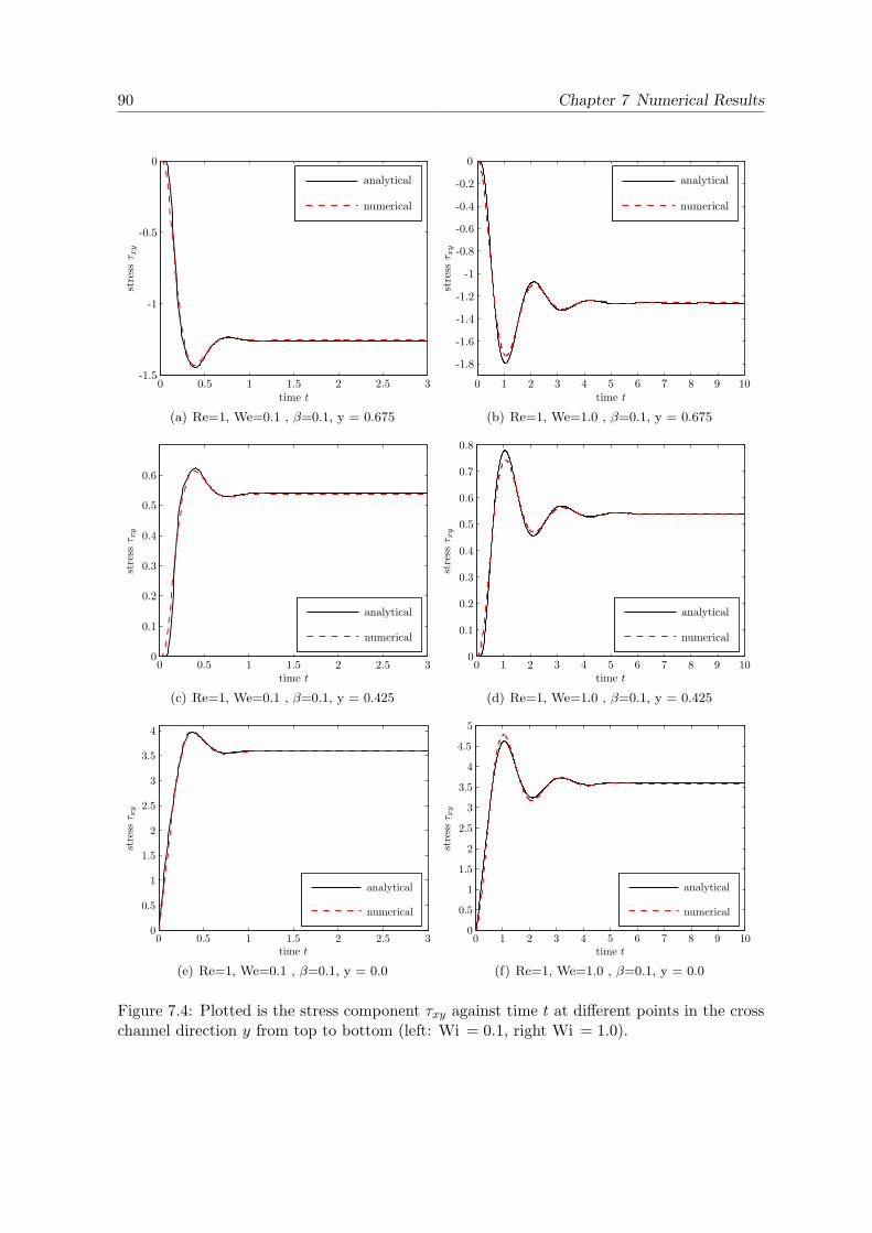
90 Chapter 7 Numerical Results
time t
stre
ssτ x
y
analytical
numerical
0 0.5 1 1.5 2 2.5 3-1.5
-1
-0.5
0
(a) Re=1, We=0.1 , β=0.1, y = 0.675
time t
stre
ssτ x
y
analytical
numerical
0 1 2 3 4 5 6 7 8 9 10
-1.8
-1.6
-1.4
-1.2
-1
-0.8
-0.6
-0.4
-0.2
0
(b) Re=1, We=1.0 , β=0.1, y = 0.675
time t
stre
ssτ x
y
analytical
numerical
0 0.5 1 1.5 2 2.5 30
0.1
0.2
0.3
0.4
0.5
0.6
0.7
(c) Re=1, We=0.1 , β=0.1, y = 0.425
time t
stre
ssτ x
y
analytical
numerical
0 1 2 3 4 5 6 7 8 9 100
0.1
0.2
0.3
0.4
0.5
0.6
0.7
0.8
(d) Re=1, We=1.0 , β=0.1, y = 0.425
time t
stre
ssτ x
y
analytical
numerical
0 0.5 1 1.5 2 2.5 30
0.5
1
1.5
2
2.5
3
3.5
4
(e) Re=1, We=0.1 , β=0.1, y = 0.0
time t
stre
ssτ x
y
analytical
numerical
0 1 2 3 4 5 6 7 8 9 100
0.5
1
1.5
2
2.5
3
3.5
4
4.5
5
(f) Re=1, We=1.0 , β=0.1, y = 0.0
Figure 7.4: Plotted is the stress component τxy against time t at different points in the crosschannel direction y from top to bottom (left: Wi = 0.1, right Wi = 1.0).

7.1 Unsteady Poiseuille Flow of an Oldroyd-B Fluid 91
Steady State Solution
In this section, we investigate the steady state solution. Here, we set the velocity at inflowand outflow to the steady state analytical expression (7.25). Furthermore, we set the stresscomponents to the steady state analytical expressions (7.28) at inflow and impose homoge-neous Neumann boundary conditions at outflow. At the channel walls, we impose no-slipboundary conditions. We observe the flow at a probe line Y over the full height of the chan-nel (0 ≤ y ≤ 1.05) at (x, z) = (5.0, 0.5) (see red line in Figure 7.1).Figure 7.5 shows the values of the velocity component u, the stress component τxx and thestress component τxy together with the respective analytic values for a resolution of thechannel of 160 × 20 × 20 and Weissenberg numbers 0.1, 0.5, 1.0, 2.0. We observe excellentagreement between the exact and the numerical solution. To confirm this impression, weexamine the quality of the approximation in a convergence study. Therefore, we calculate thesteady state solution for a Weissenberg number 0.5 on four successively refined equidistantgrids with 40 × 8 × 8, 80 × 16 × 16, 160 × 32 × 32 and 320 × 64 × 64 grid cells, which wedenote by level 1, 2, 3 and 4 respectively. Therefore, we have equidistant grids with a meshsize of h1 = h = 0.125, h2 = h/2 = 0.0625, h3 = h/4 = 0.03125 and h4 = h/8 = 0, 015625respectively. We measure the error at the probe line Y in the discrete Ll1-norm, Ll2-norm andLl∞-norm. That means, we calculate the errors by
El1(u) := ‖ ∆ul ‖Ll1=∑j
|uana(yj)− ul(yj)|hl, (7.34)
El2(u) := ‖ ∆ul ‖Ll2=√∑
j
|uana(yj)− ul(yj)|2 hl, (7.35)
El∞(u) := ‖ ∆ul ‖Ll∞= maxj
[|uana(yj)− ul(yj)|] , (7.36)
where ul(yj) is the value of the discrete numerical solution at mesh level l at position yj ,uana(yj) is the value of the analytical solution at position yj , hl is the mesh size of meshlevel l, the discrete maximum value maxj [·] and the sum is taken over all grid cells in they-direction. The results are shown in Table 7.2. With these error values, we can calculate theorder of convergence of our scheme, which is given by
pl =log(El/El+1)
log(2), (7.37)
where El and El+1 are the errors at level l and l + 1 respectively. This definition yields thedata gathered in Table 7.3, which shows the result of quadratic convergence for velocity andstress components. To complete the investigation, the behaviour of the errors is displayed asa function of the mesh size in Figure 7.6.

92 Chapter 7 Numerical Results
y
vel
oci
tyu
analytical
Wi=0.1
Wi=0.5
Wi=1
Wi=2
-0.2 0 0.2 0.4 0.6 0.8 1 1.2-0.2
0
0.2
0.4
0.6
0.8
1
1.2
(a) velocity u.
y
stre
ssτxx
analytical
Wi=0.1
analytical
Wi=0.5
analytical
Wi=1
analytical
Wi=2
-0.2 0 0.2 0.4 0.6 0.8 1 1.20
10
20
30
40
50
60
70
(b) stress τxx.
y
stre
ssτxy
analytical
Wi=0.1
Wi=0.5
Wi=1
Wi=2
-0.2 0 0.2 0.4 0.6 0.8 1 1.2-4
-2
0
2
4
(c) stress τxy.
Figure 7.5: Steady state solution at probe line Y with (0 ≤ y ≤ 1.05) and (x, z) = (5.0, 0.5).

7.1 Unsteady Poiseuille Flow of an Oldroyd-B Fluid 93
Table 7.2: Error.
Ll1-norml El1(u) El1(τxx) El1(τxy)
1 1.10−2 5.25−1 6.40−2
2 2.06−3 9.26−2 1.32−2
3 4.44−4 1.82−2 2.94−3
4 1.04−4 3.82−3 6.64−4
Ll2-norml El2(u) El2(τxx) El2(τxy)
1 1.25−2 6.85−1 6.58−2
2 2.37−3 1.29−1 1.44−2
3 5.12−4 2.59−2 3.30−3
4 1.20−4 5.62−3 7.96−4
Ll∞-norml El∞(u) El∞(τxx) El∞(τxy)
1 2.13−2 1.250 9.21−2
2 4.63−3 2.99−1 2.22−2
3 1.07−3 7.23−2 5.38−3
4 2.56−4 1.80−2 1.62−3
Table 7.3: Order of convergence, We=0.5.
u τxx τxy
order Ll1 Ll2 Ll∞ Ll1 Ll2 Ll∞ Ll1 Ll2 Ll∞
p1 2.42 2.39 2.20 2.50 2.41 2.06 2.28 2.19 2.05p2 2.21 2.21 2.12 2.35 2.32 2.05 2.17 2.12 2.05p3 2.10 2.09 2.06 2.25 2.21 2.01 2.15 2.05 1.73

94 Chapter 7 Numerical Results
h
Err
orE
(u)
Convergence u
Ll1
Ll2
Ll∞
order 2
0.01 0.110−4
10−3
10−2
10−1
(a) Velocity u.
h
Err
orE
(τxx)
Convergence τxx
Ll1
Ll2
Ll∞
order 2
0.01 0.110−3
10−2
10−1
100
101
(b) Stress component τxx.
h
Err
orE
(τxy)
Convergence τxy
Ll1
Ll2
Ll∞
order 2
0.01 0.110−4
10−3
10−2
10−1
100
(c) Stress component τxy.
Figure 7.6: Convergence of stresses and velocity.

7.2 Flow through a Rectangular Channel 95
7.2 Flow through a Rectangular Channel
In the previous section, we examined the steady state solution for the two-dimensional channelflow of an Oldroyd-B fluid. In this section, we want to investigate the three-dimensionalchannel flow with a rectangular cross section for both an Oldroyd-B and a Phan-Thien Tannerfluid. Therefore, we consider a channel of length 8.0, height 1.0 and width 1.0, which we resolveby 320× 64× 64 grid cells. We impose a parabolic velocity profile with a maximum velocityof 1.0 at inflow, which we gain from the channel flow of a Newtonian fluid. This avoidsthe occurrence of high stress values at the no-slip boundary near the inlet region, whicharise if a constant velocity value is prescribed over the whole inflow boundary. The stresstensor components are set to zero at inflow. Furthermore, homogeneous Neumann boundaryconditions are set at the outflow boundary for both velocity and stress tensor components.We impose no-slip boundary conditions at the channel walls. A summary of the relevantparameters can be found in Table 7.4. After all components have attained their steady statevalues, we examine their values at a cut in the cross channel direction at x = 5.0. Wefind that the values for the Phan-Thien Tanner model are equal for the linear form and theexponential form. This is not very surprising, since in the case of the channel flow the shearand elongation rates are not so high and therefore the linear form and the exponential formof the Phan-Thien Tanner equations predict the same behaviour (cf. Figures 3.16-3.18). InFigure 7.7, we see the parabolic velocity profile of u, the constant pressure p, the stress τxx,τxy and τxz for the Oldroyd-B model. The velocity components v,w and the stress componentsτyy, τzz, τyz have values around 10−11 and therefore, they are neglected in our investigation.For the PTT model, we obtain the same values for the velocity component u and the stresscomponents τxy and τxz (see Figure 7.8). The parabolic profile of the stress component τxx ofthe PTT model is more shallow than the parabolic profile of the stress τxx of the Oldroyd-Bmodel. Additionally, the PTT model predicts non-zero stress components τyy and τzz thatcause small velocity values v and w, which induce the stress component τyz (see Figure 7.9).The pressure reacts to those values and forms a parabolic profile.
Table 7.4: Parameters of three-dimensional channel flow.
Reynolds number 1.0Weissenberg number 0.1β 0.1ξ 0.07ε 0.25Projection method semi-implicitConvective terms VONOS

96 Chapter 7 Numerical Results
00.2
0.40.6
0.81
00.2
0.40.6
0.81
0
0.5
1
yz
vel
oci
tyu
(a) Velocity u.
00.2
0.40.6
0.81
00.2
0.40.6
0.81
−1
−0.5
0
0.5
1
yz
pressure
p
(b) Pressure p.
00.2
0.40.6
0.81
00.2
0.40.6
0.81
−1
0
1
2
3
4
yz
stress
τxx
(c) Stress component τxx.
00.2
0.40.6
0.81
00.2
0.40.6
0.81
−4
−2
0
2
4
yz
stress
τxy
(d) Stress component τxy.
00.2
0.40.6
0.81
00.2
0.40.6
0.81
−4
−2
0
2
4
yz
stress
τxz
(e) Stress component τxz.
Figure 7.7: Velocity, pressure and stresses for the Oldroyd-B model.

7.2 Flow through a Rectangular Channel 97
00.2
0.40.6
0.81
00.2
0.40.6
0.81
0
0.5
1
yz
vel
oci
tyu
(a) Velocity u.
00.2
0.40.6
0.81
00.2
0.40.6
0.810
0.05
0.1
yz
pressure
p(b) Pressure p.
00.2
0.40.6
0.81
00.2
0.40.6
0.81
−1
0
1
2
3
4
yz
stress
τxx
(c) Stress component τxx.
00.2
0.40.6
0.81
00.2
0.40.6
0.81
−4
−2
0
2
4
yz
stress
τxy
(d) Stress component τxy.
00.2
0.40.6
0.81
00.2
0.40.6
0.81
−4
−2
0
2
4
yz
stress
τxz
(e) Stress component τxz.
Figure 7.8: Velocity, pressure and stresses for the PTT model.

98 Chapter 7 Numerical Results
00.2
0.40.6
0.81
00.2
0.40.6
0.81
−0.15
−0.1
−0.05
0
yz
stress
τyy
(a) Stress component τyy.
00.2
0.40.6
0.81
00.2
0.40.6
0.81
−0.15
−0.1
−0.05
0
yz
stress
τzz
(b) Stress component τzz.
00.2
0.40.6
0.81
00.2
0.40.6
0.81
−2
−1
0
1
x 10−5
yz
vel
oci
tyv
(c) Velocity v.
00.2
0.40.6
0.81
00.2
0.40.6
0.81
−2
−1
0
1
x 10−5
yz
vel
oci
tyw
(d) Velocity w.
00.2
0.40.6
0.81
00.2
0.40.6
0.81
−0.015
−0.01
−0.005
0
0.005
0.01
yz
stress
τyz
(e) Stress component τyz.
Figure 7.9: Stresses and velocities for the PTT model.

7.3 Convergence Study on a Flow through an Infinite Channel 99
7.3 Convergence Study on a Flow through an Infinite Channel
Since to our knowledge, an analytical solution in three space dimensions for the Oldroyd-Band PTT fluid does not yet exist for both velocity and stress tensor components, we check theconvergence of our scheme by a numerical experiment. We investigate a three-dimensionalflow through an infinite channel with rectangular cross section.We choose a rectangular domain [0, 1]3 and impose periodic boundary conditions in the x-direction to build an infinite channel. The flow is driven by a gravity force of g = (10, 0, 0). Atthe walls, we impose no-slip boundary conditions. We set a constant time-step of ∆t = 0.0002,which corresponds to the time-step necessary for the computation on the finest grid. The otherparameters are chosen as listed in Table 7.5.
Table 7.5: Parameters.
Reynolds number 1.0Weissenberg number 0.1β 0.1ξ 0.07ε 0.25Projection method semi-implicitConvective terms VONOS
The discretization error can be estimated from the difference between solutions on refinedgrids. These errors can then be used to compute the order of convergence. We calculate thesteady state solution on five successively refined grids with 83, 163, 323, 643, 1283 grid cells,which we denote by level 1, 2, 3, 4 and 5 respectively. Therefore, we have equidistant grids witha mesh size of h1 = h = 0.125, h2 = h/2 = 0.0625, h3 = h/4 = 0.03125, h4 = h/8 = 0.015625and h5 = h/16 = 0.015625 respectively. We measure the error in the discrete Ll1-norm,Ll2-norm and Ll∞-norm and calculate the errors by
El1(u) := ‖ ul+1 − ul ‖Ll1=∑i,j,k
|ul+1(xi, yj , zk)− ul(xi, yj , zk)|h3l+1, (7.38)
El2(u) := ‖ ul+1 − ul ‖Ll2=√∑i,j,k
|ul+1(xi, yj , zk)− ul(xi, yj , zk)|2 h3l+1, (7.39)
El∞(u) := ‖ ul+1 − ul ‖Ll∞= maxi,j,k
[|ul+1(xi, yj , zk)− ul(xi, yj , zk)|] , (7.40)
where hl+1 is the mesh size of mesh level l+ 1 and ul+1(xi, yj , zk) is the value of the discretenumerical solution of mesh level l+1 at position (xi, yj , zk). The discrete maximum maxi,j,k[·]and the sum are taken over all grid cells of the finer mesh level l+1. To substract the discretenumerical solution ul of the coarse grid level l from the solution ul+1(xi, yj , zk) of the fine gridat position (xi, yj , zk), we have to interpolate the values of the solution ul from the coarsegrid level l to the fine grid level l + 1 for which we use the trilinear interpolation function in

100 Chapter 7 Numerical Results
three space dimension of Matlab. Then, we calculate the order of convergence by
pl =log(El/El+1)
log(2), (7.41)
where El and El+1 are the errors at level l and l + 1 respectively.The errors for the Oldroyd-B model are listed in Table 7.6 and the corresponding ordersof convergence are gathered in Table 7.7. As for the three dimensional channel flow in theprevious section, the velocity components v,w and the stress components τyy, τzz, τyz havevalues around 10−11. Therefore, we neglect these values in our study. Additionally, thepressure is only around 10−8. Therefore, we neglect the pressure as well, because 10−8 iswithin the scope of the residuum of the Poisson solver. Thus, these values are omitted in theconvergence study for the Oldroyd-B model. The components show a similar behaviour for thePTT model and the Oldroyd-B model like in the three-dimensional channel flow introducedin the previous section.We find very good convergence results for all components: the velocity u converges withan order around two and the stress components converge with an order around two in theLl1-norm and Ll2-norm and with an order of one in the Ll∞-norm. The linear convergencein the Ll∞-norm may be explained by the fact, that we calculate the values of the stressesin the corners of the boundary of the rectangular channel by linear extrapolation. Indeed,we can observe that the maximum errors occur always in these corner boundary cells. Thelinear extrapolation in the boundary corner cells does not have such a drastic influence onthe Ll1-norm and the Ll2-norm. The stress tensor components show singular behaviour towardthe corners while the velocity component has a smooth profile (see Figure 7.7). Therefore,the difference of the stress values is quite large between the coarse and the fine grid. We findthat the results match for the components τxy and τxz, which are symmetric to each other(see Figure 7.7).However, the PTT model shows the same results for the linear form and the exponential form.The linear and the exponential form predict the same behaviour for this experiment since theshear and elongation rates are not so high (see Figures 3.16-3.18). For the PTT model, wefind approximately the same results for the components u, τxx, τxy, τxz. In addition, thePTT model has a non-zero pressure, stress components τyy,τzz,τyz and velocity componentsv and w. The results for the stress components τyy and τzz match as well as the results forthe velocity components v and w. The components τyy and τzz are symmetric to each otheras well as the velocity components v and w (see Figure 7.8-7.9). The components τyy, τzzand τyz converge with an order of two in the Ll1-norm and Ll2-norm and an order between1.14 and 1.88 in the Ll∞-norm. The velocity components v and w show a convergence ratebetween 1.86 and 3.03 in the Ll1-norm and Ll2-norm and an order between 1.28 and 2.30 inthe Ll∞-norm. Finally, we can observe the convergence of the components in Figure 7.10 forthe Oldroyd-B model and in Figure 7.10 for the PTT model.

7.3 Convergence Study on a Flow through an Infinite Channel 101
Table 7.6: Error for the Oldroyd-B model.
Ll1-norml El1(u) El1(τxx) El1(τxy) El1(τxz)
1 7.06−3 3.09−2 2.38−2 2.38−2
2 1.71−3 6.39−3 4.49−3 4.49−3
3 4.34−4 1.42−3 9.50−4 9.50−4
4 1.10−4 3.31−4 2.15−4 2.15−4
Ll2-norml El2(u) El2(τxx) El2(τxy) El2(τxz)
1 7.48−3 3.17−2 4.14−2 4.14−2
2 1.89−3 7.57−3 1.01−2 1.01−2
3 4.86−4 1.93−3 2.52−3 2.52−3
4 1.23−4 4.93−4 6.36−4 6.36−4
Ll∞-norml El∞(u) El∞(τxx) El∞(τxy) El∞(τxz)
1 2.17−2 5.51−2 1.82−1 1.82−1
2 5.41−3 2.65−2 9.06−2 9.06−2
3 1.35−3 1.10−2 4.52−2 4.52−2
4 3.38−4 4.55−3 2.26−2 2.26−2
Table 7.7: Order of convergence for the Oldroyd-B model.
u τxx τxy / τxz
order Ll1 Ll2 Ll∞ Ll1 Ll2 Ll∞ Ll1 Ll2 Ll∞
p1 2.04 1.98 2.00 2.27 2.07 1.06 2.40 2.04 1.01p2 1.98 1.96 2.00 2.17 1.97 1.26 2.24 2.00 1.00p3 1.98 1.98 2.00 2.10 1.97 1.28 2.14 1.98 1.00

102 Chapter 7 Numerical Results
h
Err
orE
(u)
Convergence u
Ll1
Ll2
Ll∞
order 2
0.005 0.01 0.110−4
10−3
10−2
10−1
(a) Velocity u.
h
Err
orE
(τxx)
Convergence τxx
Ll1
Ll2
Ll∞
order 2
0.005 0.01 0.110−4
10−3
10−2
10−1
100
(b) Stress component τxx.
h
Err
orE
(τxy)
Convergence τxy/τxz
Ll1
Ll2
Ll∞
order 2
0.005 0.01 0.110−4
10−3
10−2
10−1
100
(c) Stress component τxy.
Figure 7.10: Order of convergence for stresses and velocity Oldroyd-B model.
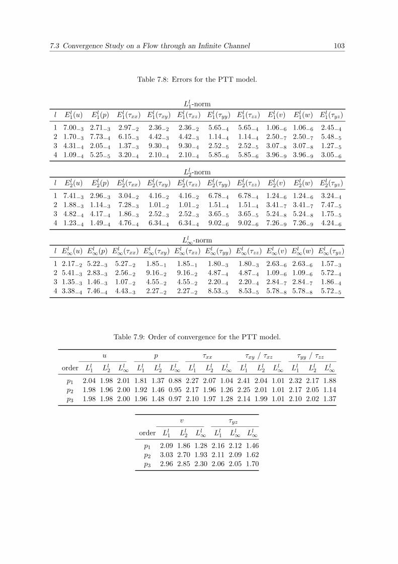
7.3 Convergence Study on a Flow through an Infinite Channel 103
Table 7.8: Errors for the PTT model.
Ll1-norml El1(u) El1(p) El1(τxx) El1(τxy) El1(τxz) El1(τyy) El1(τzz) El1(v) El1(w) El1(τyz)
1 7.00−3 2.71−3 2.97−2 2.36−2 2.36−2 5.65−4 5.65−4 1.06−6 1.06−6 2.45−4
2 1.70−3 7.73−4 6.15−3 4.42−3 4.42−3 1.14−4 1.14−4 2.50−7 2.50−7 5.48−5
3 4.31−4 2.05−4 1.37−3 9.30−4 9.30−4 2.52−5 2.52−5 3.07−8 3.07−8 1.27−5
4 1.09−4 5.25−5 3.20−4 2.10−4 2.10−4 5.85−6 5.85−6 3.96−9 3.96−9 3.05−6
Ll2-norml El2(u) El2(p) El2(τxx) El2(τxy) El2(τxz) El2(τyy) El2(τzz) El2(v) El2(w) El2(τyz)
1 7.41−3 2.96−3 3.04−2 4.16−2 4.16−2 6.78−4 6.78−4 1.24−6 1.24−6 3.24−4
2 1.88−3 1.14−3 7.28−3 1.01−2 1.01−2 1.51−4 1.51−4 3.41−7 3.41−7 7.47−5
3 4.82−4 4.17−4 1.86−3 2.52−3 2.52−3 3.65−5 3.65−5 5.24−8 5.24−8 1.75−5
4 1.23−4 1.49−4 4.76−4 6.34−4 6.34−4 9.02−6 9.02−6 7.26−9 7.26−9 4.24−6
Ll∞-norml El∞(u) El∞(p) El∞(τxx) El∞(τxy) El∞(τxz) El∞(τyy) El∞(τzz) El∞(v) El∞(w) El∞(τyz)
1 2.17−2 5.22−3 5.27−2 1.85−1 1.85−1 1.80−3 1.80−3 2.63−6 2.63−6 1.57−3
2 5.41−3 2.83−3 2.56−2 9.16−2 9.16−2 4.87−4 4.87−4 1.09−6 1.09−6 5.72−4
3 1.35−3 1.46−3 1.07−2 4.55−2 4.55−2 2.20−4 2.20−4 2.84−7 2.84−7 1.86−4
4 3.38−4 7.46−4 4.43−3 2.27−2 2.27−2 8.53−5 8.53−5 5.78−8 5.78−8 5.72−5
Table 7.9: Order of convergence for the PTT model.
u p τxx τxy / τxz τyy / τzz
order Ll1 Ll2 Ll∞ Ll1 Ll2 Ll∞ Ll1 Ll2 Ll∞ Ll1 Ll2 Ll∞ Ll1 Ll2 Ll∞
p1 2.04 1.98 2.01 1.81 1.37 0.88 2.27 2.07 1.04 2.41 2.04 1.01 2.32 2.17 1.88p2 1.98 1.96 2.00 1.92 1.46 0.95 2.17 1.96 1.26 2.25 2.01 1.01 2.17 2.05 1.14p3 1.98 1.98 2.00 1.96 1.48 0.97 2.10 1.97 1.28 2.14 1.99 1.01 2.10 2.02 1.37
v τyz
order Ll1 Ll2 Ll∞ Ll1 Ll∞ Ll∞
p1 2.09 1.86 1.28 2.16 2.12 1.46p2 3.03 2.70 1.93 2.11 2.09 1.62p3 2.96 2.85 2.30 2.06 2.05 1.70

104 Chapter 7 Numerical Results
h
Err
orE
(u)
Convergence u
Ll1
Ll2
Ll∞
order 2
0.005 0.01 0.110−4
10−3
10−2
10−1
(a) Velocity u.
h
Err
orE
(p)
Convergence p
Ll1
Ll2
Ll∞
order 2
0.005 0.01 0.110−5
10−4
10−3
10−2
10−1
(b) Pressure p.
h
Err
orE
(τxx)
Convergence τxx
Ll1
Ll2
Ll∞
order 2
0.005 0.01 0.110−4
10−3
10−2
10−1
100
(c) Stress component τxx.
h
Err
orE
(τxy)
Convergence τxy/τxz
Ll1
Ll2
Ll∞
order 2
0.005 0.01 0.110−4
10−3
10−2
10−1
100
(d) Stress component τxy/τxz.
h
Err
orE
(τyy)
Convergence τyy/τzz
Ll1
Ll2
Ll∞
order 2
0.005 0.01 0.110−6
10−5
10−4
10−3
10−2
(e) Stress component τyy/τzz.
h
Err
orE
(τyz)
Convergence τyz
Ll1
Ll2
Ll∞
order 2
0.005 0.01 0.110−6
10−5
10−4
10−3
10−2
(f) Stress component τyz.
h
Err
orE
(v)
Convergence v/w
Ll1
Ll2
Ll∞
order 2
0.005 0.01 0.110−9
10−8
10−7
10−6
10−5
(g) Velocity v/w.
Figure 7.11: Order of convergence for stresses and velocity, PTT model.

7.4 Flow over a Hole 105
7.4 Flow over a Hole
We investigate the flow of viscoelastic fluids and a Newtonian fluid over a square hole. There-fore, we consider a domain Ω = 8.0 × 4.0 × 2.0, as illustrated in Figure 7.12. We choose aresolution of 160×80×40 grid cells resulting in an equidistant grid with mesh space h = 0.05.We impose a parabolic velocity profile with a maximum velocity of one at inflow, which we
3 5 8
2
4
x
y
z
Figure 7.12: Sketch of the flow over a hole.
obtain from the simulation of a flow through a channel of a Newtonian fluid. The stresstensor components are set to zero at inflow. At outflow, we impose homogeneous Neumannboundary conditions for the velocity components and the stress tensor components. Further-more, we employ no-slip boundary conditions at the walls. We choose the parameters in thesimulation as listed in Table 7.10 and analyze the result at time t = 10 at a cut normal to thez-axis at z = 1.0. Figure 7.13 shows the numerical results for a Newtonian fluid, an Oldroyd-B fluid and different PTT fluids in comparison to experimental results obtained by Bogerand Walters [9]. The numerical results are visualized by the Line Integral Convolution (LIC)technique to present vector fields with high accuracy. In the experiment, Boger and Waltersinvestigated a Newtonian and a Boger fluid in the flow over a square hole. They observedthat for low Reynolds numbers the recirculating vortex in the hole is essentially symmetric fora Newtonian fluid (see Figure 7.13(c)), but for a viscoelastic Boger fluid the vortex is asym-metric (see Figure 7.13(d)). We were able to reproduce this result in our simulations. Whilewe obtain a symmetric vortex structure for the Newtonian fluid, we attain an asymmetric
Table 7.10: Parameters of the flow over a hole.
Reynolds number 1.0Weissenberg number 1.0β 0.1ξ 0.07ε 0.02 and 0.25Projection method semi-implicitConvective terms WENO

106 Chapter 7 Numerical Results
vortex structure for the Oldroyd-B and PTT fluids (see Figure 7.13). The Oldroyd-B fluidshows the highest asymmetry in the vortex structure and fits best to the experimental resultsof Boger and Walters. This was to be expected since Boger fluids are viscoelastic fluids witha constant shear viscosity and therefore are best represented by the Oldroyd-B fluid, whichpredicts a constant shear viscosity.Figure 7.14 shows the contour lines of the vector length of the recirculating vortex in thesquare hole. Again, we note that the Oldroyd-B model shows the highest asymmetry in thevortex. For the PTT model, we have a slight asymmetry, which increases with decreasing ε.The PTT fluid with ε = 0.25 is stronger extensional thickening and shear thinning than thePTT fluid with ε = 0.02. Furthermore, we obtain a larger vortex core for the PTT modelwith ε = 0.25 in comparison to the PTT model with ε = 0.02. We achieve similar results forthe linear and exponential PTT model. Therefore, we restrict our further investigations tothe exponential PTT model.Furthermore, we examine the stress behaviour in the overall domain. Figure 7.15 shows twocut planes normal to the x-axis through the domain. We situate the first cut near the inflowdomain and the second cut at the second corner of the hole. The cuts are shaped by thevector field and coloured by the principal stress pS, which we introduced at the beginningof this chapter. In Figure 7.15, we see that the principal stress values are smaller for thePTT model than for the Oldroyd-B model and that the principal stress has its highest valuesnear the no-slip boundary and its lowest values in the middle of the cuts. We observe theconnection between the velocity gradient and principal stress: the higher the velocity gra-dient, the higher the values of the principal stress. In Figures 7.16-7.18, we colour the cutnormal to the z-axis at z = 1.0 by velocities and stresses. The Oldroyd-B model has veryhigh values of shear, normal and principal stress at the corner singularities, especially at thesecond corner of the hole. The shear, normal and principal stresses sharpen much less rapidlyfor the exponential PTT model. We get the smoothest results with the exponential PTTmodel with ε = 0.25. This confirms the theoretical findings of Renardy [61] concerning thedifferent thicknesses of boundary layers for different models. The difficulty of resolving thesteep stress gradients near the boundary and especially near corner singularities is one reasonfor the numerical breakdown in simulations of viscoelastic fluids. Figure 7.19 illustrates howsteep and dramatic these stress gradients are at the corners. Here, we plot the elastic stresstensor components along a probe line, displayed as the red line in the sketch 7.19(a). Thestress gradients are dramatically steep for the Oldroyd-B model. For the PTT model, thestress components show a much smoother behaviour especially with increasing ε.

7.4 Flow over a Hole 107
(a) Newtonian, Re=1 (b) Oldroyd-B, Re=1, We=1, β = 0.1
(c) Newtonian Fluid Experiment (d) Boger Fluid Experiment
(e) Exponential PTT, Re=1, We=1, β = 0.1, ε =0.25, ξ = 0.07
(f) Exponential PTT, Re=1, We=1, β = 0.1, ε =0.02, ξ = 0.07
(g) Linear PTT, Re=1, We=1, β = 0.1, ε = 0.25,ξ = 0.07
(h) Linear PTT, Re=1, We=1, β = 0.1, ε = 0.02,ξ = 0.07
Figure 7.13: Numerical results in comparison with experimental results for a flow over a hole,((c), (d) are from D. V. Boger and K. Walters [9]). The numerical results are shown at a cutnormal to the z-axis at z = 1.0 and they are visualized by the LIC technique.
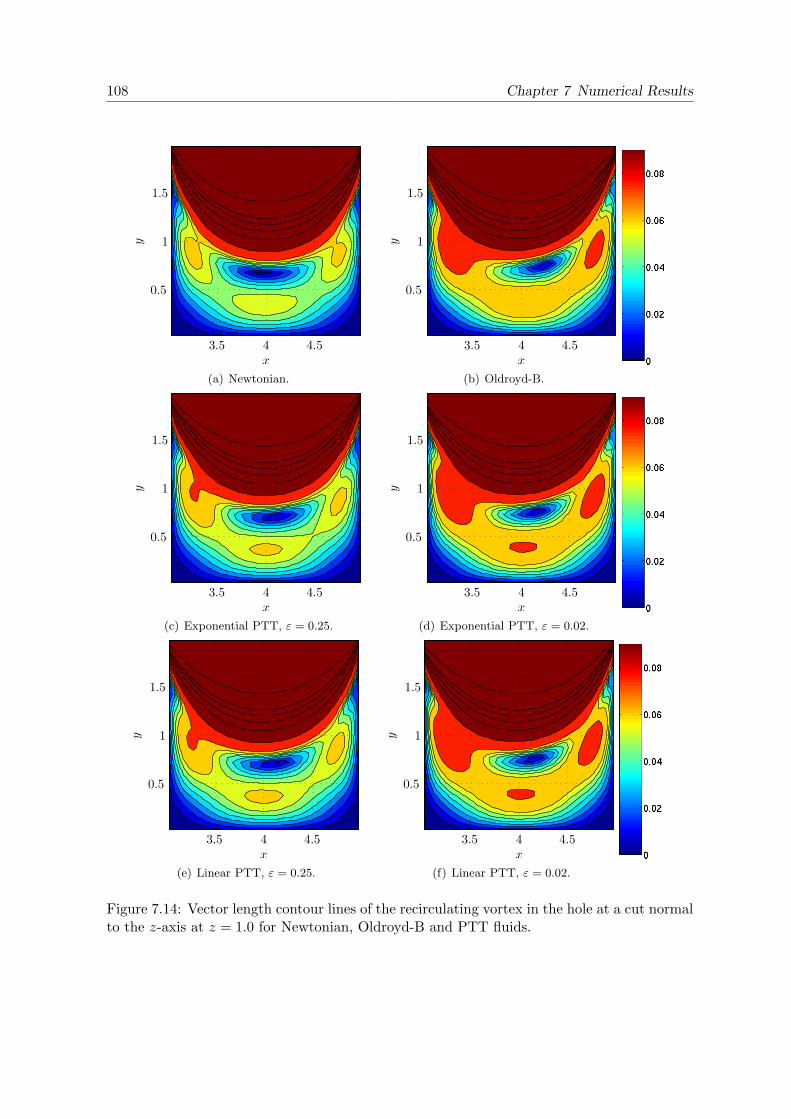
108 Chapter 7 Numerical Results
x
y
3.5 4 4.5
0.5
1
1.5
(a) Newtonian.
x
y
3.5 4 4.5
0.5
1
1.5
(b) Oldroyd-B.
x
y
3.5 4 4.5
0.5
1
1.5
(c) Exponential PTT, ε = 0.25.
x
y
3.5 4 4.5
0.5
1
1.5
(d) Exponential PTT, ε = 0.02.
x
y
3.5 4 4.5
0.5
1
1.5
(e) Linear PTT, ε = 0.25.
x
y
3.5 4 4.5
0.5
1
1.5
(f) Linear PTT, ε = 0.02.
Figure 7.14: Vector length contour lines of the recirculating vortex in the hole at a cut normalto the z-axis at z = 1.0 for Newtonian, Oldroyd-B and PTT fluids.

7.4 Flow over a Hole 109
(a) Oldroyd-B, back. (b) Oldroyd-B, front.
(c) Exponential PTT, ε = 0.25, back. (d) Exponential PTT, ε = 0.25, front.
Figure 7.15: Cut planes in shape of the velocity vector field coloured by the principal stressfor the Oldroyd-B and exponential PTT fluid.
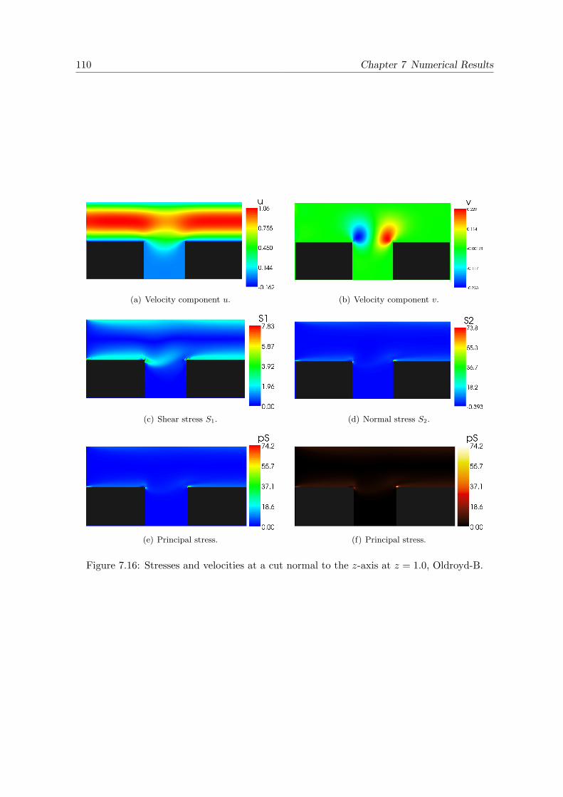
110 Chapter 7 Numerical Results
(a) Velocity component u. (b) Velocity component v.
(c) Shear stress S1. (d) Normal stress S2.
(e) Principal stress. (f) Principal stress.
Figure 7.16: Stresses and velocities at a cut normal to the z-axis at z = 1.0, Oldroyd-B.

7.4 Flow over a Hole 111
(a) Velocity component u. (b) Velocity component v.
(c) Shear stress S1. (d) Normal stress S2.
(e) Principal stress. (f) Principal stress.
Figure 7.17: Stresses and velocities at a cut normal to the z-axis at z = 1.0, exponential PTTε = 0.02.

112 Chapter 7 Numerical Results
(a) Velocity component u. (b) Velocity component v.
(c) Shear stress S1. (d) Normal stress S2.
(e) Principal stress. (f) Principal stress.
Figure 7.18: Stresses and velocities at a cut normal to the z-axis at z = 1.0, exponential PTTε = 0.25.

7.4 Flow over a Hole 113
0 3 5 8x
(a) Sketch.
Oldroyd-B
EPTT ε = 0.02
EPTT ε = 0.25
LPTT ε = 0.02
LPTT ε = 0.25
(b) Legend.
x
stress
τxx
0 1 2 3 4 5 6 7 8
0
20
40
60
80
100
(c) Stress component τxx.
x
stress
τyy
0 1 2 3 4 5 6 7 8
-6
-5
-4
-3
-2
-1
0
1
2
3
(d) Stress component τyy.
x
stress
τzz
0 1 2 3 4 5 6 7 8
-0.04
-0.02
0
0.02
0.04
0.06
(e) Stress component τzz.
x
stress
τxy
0 1 2 3 4 5 6 7 8
-2
-1
0
1
2
3
4
5
6
7
(f) Stress component τxy.
x
stress
τxz
0 1 2 3 4 5 6 7 8
-1
-0.8
-0.6
-0.4
-0.2
0
0.2
0.4
(g) Stress component τxz.
x
stress
τzz
0 1 2 3 4 5 6 7 8
-0.04
-0.02
0
0.02
0.04
0.06
(h) Stress component τyz.
Figure 7.19: Behaviour of the elastic stress tensor components near the corner singularities.

114 Chapter 7 Numerical Results
7.5 Karman Vortex Street
We investigate the flow past an inclined plate, which results in a Karman Vortex Street. Weconsider a domain Ω = 60.0×12.0×6.0, which we resolve by 300×60×30 grid cells resultingin an equidistant grid with a mesh size of 0.2 (see Figure 7.20). We set periodic boundaryconditions in the z-direction to simulate an infinite domain in this direction. Therefore, wecan set the analytical steady state expressions (7.25) and (7.25) for the velocity and the stresscomponents at inflow. At outflow, we set homogeneous Neumann boundary conditions. Theinclined plate is placed in the domain as illustrated in Figure 7.20. The remaining parametersare gathered in Table 7.11. We examine the vortex street at time t = 160 and at a cut normalto the z-axis at z = 3.
x
y
z
60
12
0 3 5 8
(a) Dimensions and position of the inclined plate.
z
y6
12
0 2 4
4.5
7.5
(b) Dimensions andposition of the in-clined plate in the yz-plane.
Figure 7.20: Sketch of the Karman vortex street problem.
We investigate the Karman Vortex Street for a Newtonian fluid, an Oldroyd-B fluid andPTT fluids with ε = 0.25 and ε = 0.02 for both the linear form and the exponential form.Figure 7.21 shows pictures from a laboratory experiment of the vortex shedding behind acylinder for a Newtonian fluid and a dilute polymer solution obtained by Boger and Walters[9]. We observe that adding even small amounts of a dissolved polymer to a Newtonian fluidleads to different vortex shedding behaviour.
Table 7.11: Parameters of Karman vortex street.
Reynolds number 400Weissenberg number 0.5β 0.1ξ 0.07ε 0.02 and 0.25Projection method explicitConvective terms VONOS

7.5 Karman Vortex Street 115
(a) Newtonian, water
(b) Viscoelastic, 50 ppm aqueous solution of polyacrylamide (AP 45)
Figure 7.21: Vortex shedding behind a cylinder (from D. V. Boger and K. Walters [9])
Compared to the purely Newtonian solvent, the viscoelastic fluid shows a reduction in fre-quency of vortex shedding, an increased length of the formation region just behind the cylin-der, and an alteration of the form of the relative vorticity patterns. These observations canbe explained by the higher elongational viscosity of an elastic liquid and by the suppressionof velocity fluctuations by elasticity.We could observe the same qualitative behaviour in our simulations. Figure 7.22 shows anLIC picture of the Karman vortex street coloured by the vector length and Figure 7.23 showsthe contour lines of the vector length. We observe that the vortices behind the inclined platehave an increased length for all viscoelastic fluids. The Oldroyd-B fluid shows the strongestelongation of the vortices. Additionally, the Oldroyd-B fluid exhibits the strongest suppressionof velocity fluctuations. The PTT fluids with ε = 0.02 show also a considerable suppressionof velocity fluctuations, while the PTT fluids with ε = 0.25 show only a slight suppression.This could be caused by the stronger shear-thinning of PTT fluids with ε = 0.25.In Figure 7.24, we observe the principal stress behaviour of the different viscoelastic fluids.The models show a very high stress concentration on the upper left corner of the inclinedplate. Especially, the Oldroyd-B model predicts a high stress peak at that corner. Table 7.13gathers the minimum and the maximum values of the velocity components and the stresscomponents of the different models. We see that the Oldroyd-B model predicts dramaticallyhigh values for the stress components τxx, τyy and τxy, while the PTT model predicts mod-erate stress values and the principal stress values decrease with increasing ε. The biggestcontrast is between the Oldroyd-B model and the exponential PTT model with ε = 0.25.Therefore, we choose these two models for further comparisons. In Figure 7.25 and Figure 7.26,we compare the contour plots of the velocity components and the pressure for the Newtonianfluid, the Oldroyd-B fluid and the exponential PTT fluid. Figure 7.27 shows the normal stresscomponents, Figure 7.28 the shear stress components and Figure 7.29 the normal, shear and

116 Chapter 7 Numerical Results
Table 7.12: Maximum values of the velocity and the pressure (ε1 = 0.02, ε2 = 0.25).
u v w p
Min Max Min Max Min Max Min Max
Newton -1.00 1.72 -1.00 1.09 -0.52 0.44 -1.26 0.77Old-B -1.19 1.65 -1.02 0.96 -0.54 0.45 -0.91 1.33EPTT ε1 -1.12 1.75 -1.00 0.99 -0.63 0.59 -1.40 1.28LPTT ε1 -1.11 1.69 -1.00 1.05 -0.55 0.46 -0.94 0.91EPTT ε2 -1.12 1.79 -1.00 1.10 -0.56 0.48 -1.46 1.35LPTT ε2 -1.11 1.74 -0.99 1.03 -0.58 0.57 -0.91 0.89
Table 7.13: Maximum values of the stress components (ε1 = 0.02, ε2 = 0.25).
τxx τyy τzz τxy τxz τyz pS
Min Max Min Max Min Max Min Max Min Max Min Max Min Max
Old-B -262.05 258.85 -149.07 202.75 -3.50 4.81 -114.17 115.91 -17.87 17.80 -10.42 10.21 0.00 300.63EPTT ε1 -22.17 37.23 -22.02 24.17 -3.00 6.01 -6.76 3.77 -4.77 5.70 -3.03 2.87 0.00 41.88LPTT ε1 -24.40 37.56 -23.26 25.80 -3.02 5.06 -8.72 4.86 -5.24 5.77 -3.02 2.85 0.00 42.24EPTT ε2 -1.18 16.23 -5.83 5.98 -2.20 3.96 -1.18 16.23 -4.56 4.54 -2.87 2.81 0.00 19.54LPTT ε2 -3.09 20.97 -7.19 7.51 -2.28 3.55 -3.09 20.97 -4.81 4.80 -3.03 2.96 0.00 24.29
principal stress measures. The Figures illustrate the above mentioned differences between thefluids and we see significant differences between them in all components.

7.5 Karman Vortex Street 117
(a) Newtonian.
(b) Oldroyd-B.
(c) Exponential PTT, ε = 0.25.
(d) Exponential PTT, ε = 0.02.
(e) Linear PTT, ε = 0.25.
(f) Linear PTT, ε = 0.02.
Figure 7.22: LIC picture of the Karman vortex street coloured by the vector length ‖ u ‖.

118 Chapter 7 Numerical Results
x
y
0 10 20 30 40 50 600
5
10
(a) Newtonian.
x
y
0 10 20 30 40 50 600
5
10
(b) Oldroyd-B.
x
y
0 10 20 30 40 50 600
5
10
(c) Exponential PTT, ε = 0.25.
x
y
0 10 20 30 40 50 600
5
10
(d) Exponential PTT, ε = 0.02.
x
y
0 10 20 30 40 50 600
5
10
(e) Linear PTT, ε = 0.25.
x
y
0 10 20 30 40 50 600
5
10
(f) Linear PTT, ε = 0.02.
Figure 7.23: Contour lines of the Karman vortex street of the vector length ‖ u ‖.

7.5 Karman Vortex Street 119
(a) Oldroyd-B.
(b) Exponential PTT, ε = 0.25.
(c) Exponential PTT, ε = 0.02.
(d) Linear PTT, ε = 0.25.
(e) Linear PTT, ε = 0.02.
Figure 7.24: LIC picture of the Karman vortex street coloured by the priniciple stress pS.

120 Chapter 7 Numerical Results
(a) Newtonian, velocity component u.
(b) Exponential PTT, ε = 0.25, velocity component u.
(c) Oldroyd-B, velocity component u.
(d) Newtonian, velocity component v.
(e) Exponential PTT, ε = 0.25, velocity component v.
(f) Oldroyd-B, velocity component v.
Figure 7.25: Velocity components u and v for the Karman vortex street.

7.5 Karman Vortex Street 121
(a) Newtonian, velocity component w.
(b) Exponential PTT, ε = 0.25, velocity component w.
(c) Oldroyd-B, velocity component w.
(d) Newtonian, pressure p.
(e) Exponential PTT, ε = 0.25, pressure p.
(f) Oldroyd-B, pressure p.
Figure 7.26: Velocity component w and pressure p for the Karman vortex street.

122 Chapter 7 Numerical Results
(a) Exponential PTT, ε = 0.25, stress tensor component τxx.
(b) Oldroyd-B, stress tensor component τxx.
(c) Exponential PTT, ε = 0.25, stress tensor component τxx.
(d) Oldroyd-B, stress tensor component τyy.
(e) Exponential PTT, ε = 0.25, stress tensor component τzz.
(f) Oldroyd-B, stress tensor component τzz.
Figure 7.27: Normal stress components for the Oldroyd-B model and the exponential PTTmodel for the Karman vortex street.

7.5 Karman Vortex Street 123
(a) Exponential PTT, ε = 0.25, stress tensor component τxy.
(b) Oldroyd-B, stress tensor component τxy.
(c) Exponential PTT, ε = 0.25, stress tensor component τxz.
(d) Oldroyd-B, stress tensor component τxz.
(e) Exponential PTT, ε = 0.25, stress tensor component τyz.
(f) Oldroyd-B, stress tensor component τyz.
Figure 7.28: Shear stress components for the Oldroyd-B model and the exponential PTTmodel for the Karman vortex street.

124 Chapter 7 Numerical Results
(a) Exponential PTT, ε = 0.25, shear stress S1.
(b) Oldroyd-B, shear stress S1.
(c) Exponential PTT, ε = 0.25, normal stress S2.
(d) Oldroyd-B, normal stress S2.
(e) Exponential PTT, ε = 0.25, principal stress pS.
(f) Oldroyd-B, principal stress pS.
Figure 7.29: Normal and shear stress S1 and S2, and principal stress pS for the Oldroyd-Bmodel and the exponential PTT model for the Karman vortex street.

Chapter 8
Conclusion
Summary
The main aim of this thesis was to develop a numerical method for solving transientviscoelastic flow problems in three space dimensions. To this end, we chose the Oldroyd-Bequations and both the exponential form and the linear form of the Phan-Thien Tannerequations including the prediction of non-affine motion and a Newtonian contribution tothe stress tensor to model viscoelasticity. Before, we used these models in our simulations,we investigated their predictions of shear-dependent viscosity, normal stress differences andelongational viscosity and discussed the meaning of their parameters very thoroughly.To solve the equations, describing the flow of a viscoelastic fluid, we discretized the unknownson a staggered grid, where the pressure and the stress tensor components were discretized inthe centre of the cells, while the velocities were discretized at the cell sides. We discretizedthe spatial derivatives in the Oldroyd-B and the Phan-Thien Tanner equations by centraldifferences except for the convective terms, for which we employed the VONOS schemeand the WENO scheme. Moreover, we implemented Dirichlet, homogeneous Neumann andno-slip boundary conditions for the stress tensor components. We extended the Navier-Stokesequations by the parameter β in front of the diffusive terms and by the addition of thedivergence of the elastic stress tensor, which we discretized by central differences. For thetemporal discretization, we employed a Chorin-type projection method and a semi-implicitprojection method with implicit treatment of the diffusive terms. Furthermore, we acceler-ated our computations by parallelization using a domain decomposition method.In our computations, we could observe significant differences in the flow behaviour of theOldroyd-B fluid and the Phan-Thien Tanner fluids. To investigate the differences of theirstress predictions, we computed a flow directed shear and normal stress to obtain a physicallymeaningful stress measure in complex flows and used these stress measures to compute aprincipal stress. In our investigations of the principal stress, we found that the Oldroyd-Bfluids show very thin stress boundary layers near the no-slip boundary, while the stressboundary layers occurring in PTT fluids are much wider.We validated our implementations by the investigation of the numerical approximation ofthe analytical solution of the transient plane Poiseuille flow of an Oldroyd-B fluid and by aconvergence study of a three-dimensional gravity driven flow through an infinite rectangularchannel. We found an excellent agreement between the transient analytical solution and thenumerical solution for the velocities and the stress tensor components and we observed thatthe numerical solution converged quadratically to the steady state analytical solution withmesh refinement. We also found quadratic convergence of all components in the convergencestudy of the three-dimensional gravity driven flow through an infinite rectangular channel

126 Chapter 8 Conclusion
for the Oldroyd-B model and the PTT model.Furthermore, we examined the flow through a three-dimensional rectangular channel, theflow over a hole and the Karman vortex street behind an inclined plate and investigated theresults for the different models. For the flow through a three-dimensional rectangular channel,we plotted and compared the velocity and stress tensor components for the different models.In the flow over a hole, we could observe an asymmetric vortex structure for the Oldroyd-Bfluid and the PTT fluids, as seen in experiments with viscoelastic fluids. In addition,we could observe that the Oldroyd-B model showed extremely steep stress gradients atcorner singularities, while the stress gradients for the PTT models were much less dramatic.Moreover, we investigated a Karman vortex street behind an inclined plate for the differentmodels. We were able to observe different vortex stretching behaviour and suppressionof velocity fluctuations as seen in laboratory experiments. We found that the Oldroyd-Bmodel suppresses velocity fluctuations in a very strong manner and leads to the strongestelongation of the vortices behind the inclined plate. To our knowledge, the Karman vortexstreet behind an inclined plate, has not yet been numerically investigated for viscoelastic flows.
Outlook
Even though, we were able to simulate three-dimensional transient viscoelastic complex flowsituations for different viscoelastic materials, there is still much room for further research andpossible extensions.To aim for numerical simulations of flows with higher Weissenberg numbers, we could employan adaptive grid refinement scheme, which refines the grid in high deformation regions as toobey the stability criterion on the mesh size ∆x ≤ | u | /(2
√−det(∇u) −Wi−1) of Fattal
and Kupferman [22, 23]. Additionally, a refinement of the regions near no-slip boundariesand corner singularities in order to resolve the boundary layers and the steep stress gradientscould stabilize the calculations.An extension to two phase flows would give the opportunity to investigate the numerous fasci-nating free surface phenomena such as die-swell or the Weissenberg effect. Moreover, in orderto simulate industrial processes it is inevitable to consider free surface flows. However, theextension to free surface flows is not straightforward since researchers investigate instabilitiesnear the free surface, which have to be prevented by appropriate numerical schemes (see e.g.Khismatullin [41]).Moreover, it would be interesting to implement other differential constitutive equations likethe Giesekus model, the Pom-Pom model and the eXtended Pom-Pom model to be able tosimulate a wider variety of viscoelastic liquids.

Appendix A
Components of the Governing Equations
Vectors
u = (u, v, w) (A.1)
g = (gx, gy, gz) (A.2)
Tensors
D =
∂u∂x
12(∂u∂y + ∂v
∂x) 12(∂u∂z + ∂w
∂x )12(∂u∂y + ∂v
∂x) ∂v∂y
12(∂v∂z + ∂w
∂y )12(∂u∂z + ∂w
∂x ) 12(∂v∂z + ∂w
∂y ) ∂w∂z
(A.3)
τττ =
τxx τxy τxzτyx τyy τyzτzx τzy τzz
(A.4)
∇u =
∂u∂x
∂u∂y
∂u∂z
∂v∂x
∂v∂y
∂v∂z
∂w∂x
∂w∂y
∂w∂z
(A.5)
Momentum Equation
x-component
∂u
∂t+∂(u2)∂x
+∂(uv)∂y
+∂(uw)∂z
= −∂p∂x
+1
Reβ
[∂2u
∂x2+∂2u
∂y2+∂2u
∂z2
]+
1Re
[∂τxx∂x
+∂τxy∂y
+∂τxz∂z
]+
1Fr2 gx
(A.6)

128 Appendix A Components of the Governing Equations
y-component
∂v
∂t+∂(uv)∂x
+∂(v2)∂y
+∂(vw)∂z
= −∂p∂y
+1
Reβ
[∂2v
∂x2+∂2v
∂y2+∂2v
∂z2
]+
1Re
[∂τyx∂x
+∂τyy∂y
+∂τyz∂z
]+
1Fr2 gy
(A.7)
z-component
∂w
∂t+∂(uw)∂x
+∂(vw)∂y
+∂(w2)∂z
= −∂p∂z
+1
Reβ
[∂2w
∂x2+∂2w
∂y2+∂2w
∂z2
]+
1Re
[∂τzx∂x
+∂τzy∂y
+∂τzz∂z
]+
1Fr2 gz
(A.8)
Phan-Thien Tanner Equation
xx-component
f(trτττ)τxx + Wi∂τxx∂t
+ u∂τxx∂x
+ v∂τxx∂y
+ w∂τxx∂z
+ Wi
2(ξ − 1)
∂u
∂xτxx +
[(ξ − 2)
∂u
∂y+ ξ
∂v
∂x
]τxy +
[(ξ − 2)
∂u
∂z+ ξ
∂w
∂x
]τxz
= 2(1− β)
∂u
∂x
(A.9)
yy-component
f(trτττ)τyy + Wi∂τyy∂t
+ u∂τyy∂x
+ v∂τyy∂y
+ w∂τyy∂z
+ Wi
[(ξ − 2)
∂v
∂x+ ξ
∂u
∂y
]τxy + 2(ξ − 1)
∂v
∂yτyy +
[(ξ − 2)
∂v
∂z+ ξ
∂w
∂y
]τyz
= 2(1− β)
∂v
∂y
(A.10)
zz-component
f(trτττ)τzz + Wi∂τzz∂t
+ u∂τzz∂x
+ v∂τzz∂y
+ w∂τzz∂z
+ Wi
[(ξ − 2)
∂w
∂x+ ξ
∂u
∂z
]τxz +
[(ξ − 2)
∂w
∂y+ ξ
∂v
∂z
]τyz + 2(ξ − 1)
∂w
∂zτzz
= 2(1− β)
∂w
∂z
(A.11)
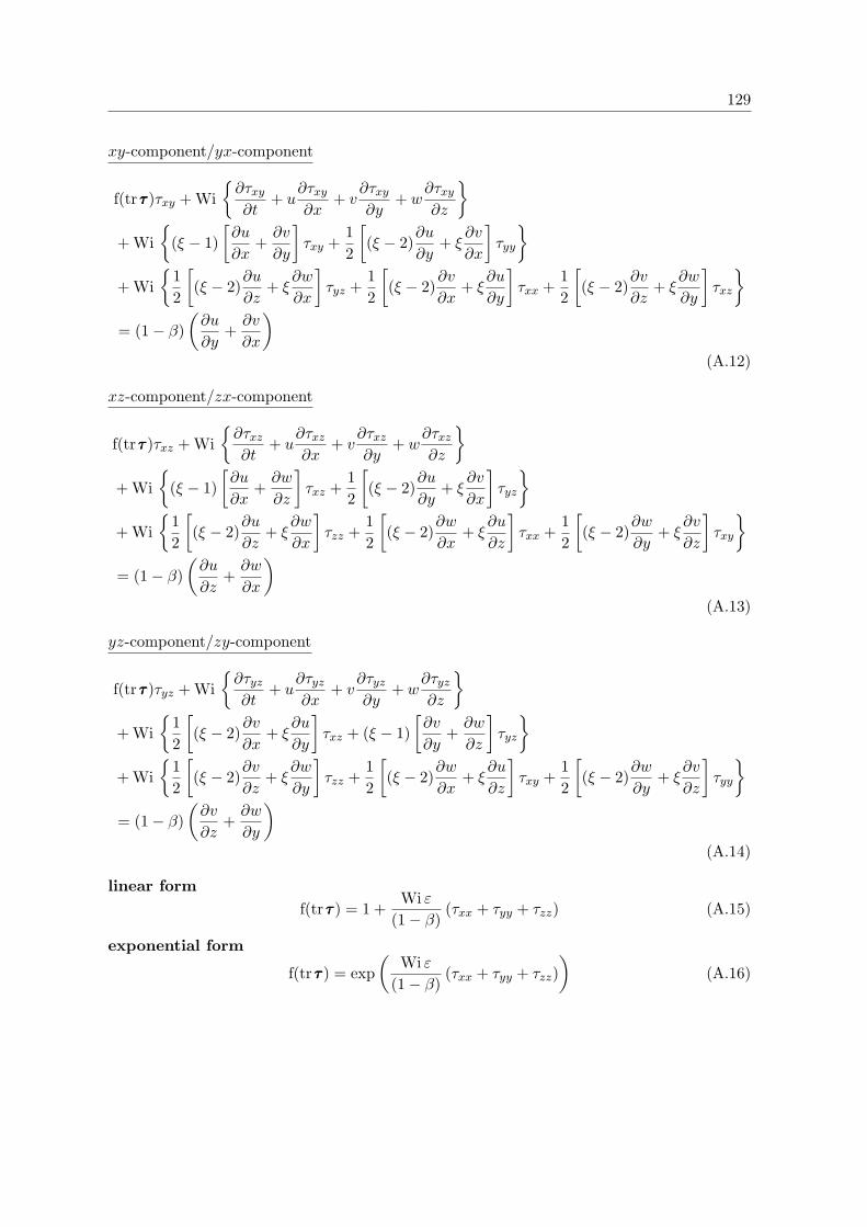
129
xy-component/yx-component
f(trτττ)τxy + Wi∂τxy∂t
+ u∂τxy∂x
+ v∂τxy∂y
+ w∂τxy∂z
+ Wi
(ξ − 1)
[∂u
∂x+∂v
∂y
]τxy +
12
[(ξ − 2)
∂u
∂y+ ξ
∂v
∂x
]τyy
+ Wi
12
[(ξ − 2)
∂u
∂z+ ξ
∂w
∂x
]τyz +
12
[(ξ − 2)
∂v
∂x+ ξ
∂u
∂y
]τxx +
12
[(ξ − 2)
∂v
∂z+ ξ
∂w
∂y
]τxz
= (1− β)
(∂u
∂y+∂v
∂x
)(A.12)
xz-component/zx-component
f(trτττ)τxz + Wi∂τxz∂t
+ u∂τxz∂x
+ v∂τxz∂y
+ w∂τxz∂z
+ Wi
(ξ − 1)
[∂u
∂x+∂w
∂z
]τxz +
12
[(ξ − 2)
∂u
∂y+ ξ
∂v
∂x
]τyz
+ Wi
12
[(ξ − 2)
∂u
∂z+ ξ
∂w
∂x
]τzz +
12
[(ξ − 2)
∂w
∂x+ ξ
∂u
∂z
]τxx +
12
[(ξ − 2)
∂w
∂y+ ξ
∂v
∂z
]τxy
= (1− β)
(∂u
∂z+∂w
∂x
)(A.13)
yz-component/zy-component
f(trτττ)τyz + Wi∂τyz∂t
+ u∂τyz∂x
+ v∂τyz∂y
+ w∂τyz∂z
+ Wi
12
[(ξ − 2)
∂v
∂x+ ξ
∂u
∂y
]τxz + (ξ − 1)
[∂v
∂y+∂w
∂z
]τyz
+ Wi
12
[(ξ − 2)
∂v
∂z+ ξ
∂w
∂y
]τzz +
12
[(ξ − 2)
∂w
∂x+ ξ
∂u
∂z
]τxy +
12
[(ξ − 2)
∂w
∂y+ ξ
∂v
∂z
]τyy
= (1− β)
(∂v
∂z+∂w
∂y
)(A.14)
linear formf(trτττ) = 1 +
Wi ε(1− β)
(τxx + τyy + τzz) (A.15)
exponential form
f(trτττ) = exp(
Wi ε(1− β)
(τxx + τyy + τzz))
(A.16)

130 Appendix A Components of the Governing Equations
Continuity Equation
∂u
∂x+∂v
∂y+∂w
∂z= 0 (A.17)

Appendix B
Analytical Solution of the Poiseuille Flow of anOldroyd-B Fluid
In this section, we will describe the derivation of the expressions for the stress tensor compo-nents using the analytical solution of Waters and King [73]. The analytical solution of Watersand King can be written as
u(y, t) = 4y(1− y)− 32∞∑n=1
sin(Ny)N3
GN (El, t), (B.1)
where
N = (2n− 1)π, A(y) = 4y(1− y), (B.2)
αN = 1 + ElN2 β2N = α2
N − 4N2El, βN =√βN , (B.3)
γN = 1 +N2El(β − 2), α∗N =αN2El
, β∗N =βN2El
(B.4)
aN = 1 +γNβN
, bN = 1− γNβN
, pN = −α∗N + β∗N , qN = −α∗N − β∗N ,
(B.5)
and
GN (El, t∗) =
12 [aN exp (pN t) + bN exp (qN t)] if β2
N ≥ 0,
exp (−α∗N t)[cos (β∗N t) + γN
βNsin (β∗N t)
]if β2
N < 0.(B.6)
For the Poiseuille Flow all derivatives in the channel direction (x) are zero and v = 0. There-fore, the equations for the elastic stress tensor components reduce to
τxx + El∂τxx∂t
= 2Wi∂u
∂yτxy, (B.7)
τxy + El∂τxy∂t
= (1− β)∂u
∂y+ Wi
∂u
∂yτyy, (B.8)
τyy + El∂τyy∂t
= 0, (B.9)
when the non-dimensionalization of Waters and King (7.14) is used. To solve these equations,let us introduce the change of variables
τττ = exp(− t
El
)∼τττ . (B.10)

132 Appendix B Analytical Solution of the Poiseuille Flow of an Oldroyd-B Fluid
By introducing (B.10) into (B.7) - (B.9), we obtain
∂∼τ xx∂t
= 2Re∂u
∂y
∼τ xy, (B.11)
∂∼τ xy∂t
=(1− β)
El∂u
∂yexp
(t
El
)+ Re
∂u
∂y
∼τ yy, (B.12)
∂∼τ yy∂t
= 0. (B.13)
With the initial conditionτττ = 0 at t = 0, (B.14)
we obtainτyy = 0. (B.15)
Therefore, equation (B.12) reduces to
∂∼τ xy∂t
=(1− β)
El∂u
∂yexp
(t
El
), (B.16)
which gives on integration over [0, t]
∼τ xy(t)−
∼τ xy(0) =
(1− β)El
∫ t
0
∂u
∂yexp
(t
El
)dt. (B.17)
The derivative of the velocity component is given by
∂u
∂y= A′(y)− 32
∞∑n=1
cos(Ny)N2
GN (El, t), (B.18)
whereA′(y) =
dA(y)dy
= 4(1− 2y). (B.19)
After integration, and with∼τ xy(0) = 0, we obtain
∼τ xy(t) =
(1− β)El
exp(t
El
)[ElA′(y)− 32
∞∑n=1
cos(Ny)N2
HN (El, t)
]+ Cxy(El, y), (B.20)
where Cxy(El, y) is the sum of the results of the integrals for t = 0 and
HN (El, t∗) =
12
[aN
pN + 1/Elexp (pN t) +
bNqN + 1/El
exp (qN t)]
if β2N ≥ 0,
exp (−α∗N t)cN
[(β∗N + hN
γNβN
)sin (β∗N t) +
(hN − β∗N
γNβN
)cos (β∗N t)
]if β2
N < 0
(B.21)with
hN = −α∗N +1El, cN = h2
N + (β∗N )2. (B.22)

133
Finally, by multiplying equation (B.20) with exp(−t/El), we obtain
τxy(t) =(1− β)
El
[ElA′(y)− 32
∞∑n=1
cos(Ny)N2
HN (El, t)
]+ Cxy(El, y) exp
(− t
El
). (B.23)
Now, we can calculate the expression for τxx with
∼τ xx(t) = 2Re
∫ t
0
∂u
∂y
∼τ xy dt. (B.24)
With (B.20) and (B.20) this yields
∼τ xx(t) = 2ReCxy(El, y)
[A′(y)
∫ t
0dt− 32
∞∑n=1
cos(Ny)N2
∫ t
0GN (El, t) dt
]
+ 2Re (1− β)A′(y)
[A′(y)El exp
(t
El
)− 32
∞∑n=1
cos(Ny)N2
∫ t
0GN (El, t) exp
(t
El
)dt
]
− 64 ReA′(y)(1− β)El
∞∑n=1
cos(Ny)N2
∫ t
0HN (El, t) exp
(t
El
)dt
+2 · 322 Re (1− β)
El
∞∑n,m=1
cos(Ny)N2
cos(My)M2
∫ t
0HN (El, t)GM (El, t) exp
(t
Eldt
).
(B.25)
Integrating and multiplying by exp(−t/El) results in
τxx(t) = 2ReCxy(El, y)
[A′(y) exp
(− t
El
)t− 32
∞∑n=1
cos(Ny)N2
IN (El, t)
]
+ 2Re (1− β)A′(y)
[A′(y)El− 32
∞∑n=1
cos(Ny)N2
HN (El, t)
]
− 64 ReA′(y)(1− β)El
∞∑n=1
cos(Ny)N2
JN (El, t)
+2 · 322 Re (1− β)
El
∞∑n,m=1
cos(Ny)N2
cos(My)M2
KNM (El, t) + Cxx(El, y) exp(− t
El
),
(B.26)
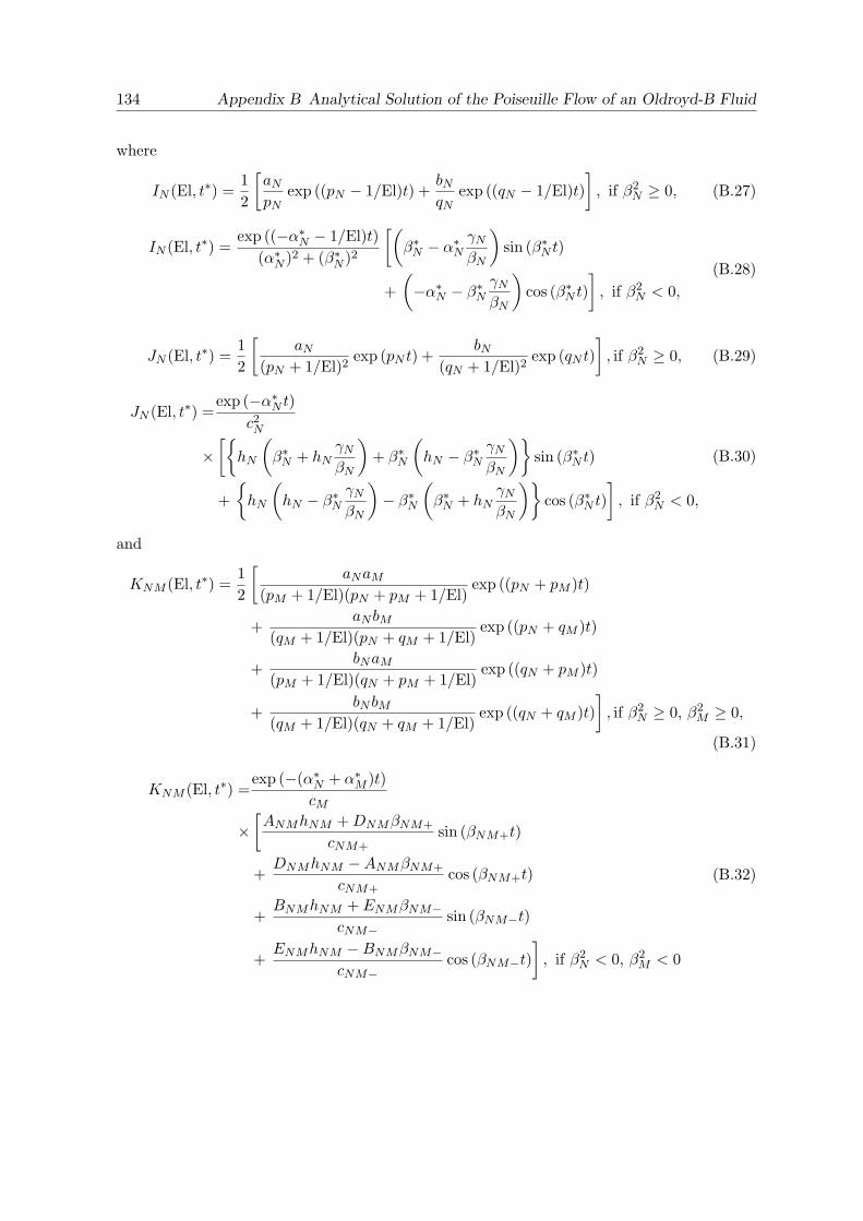
134 Appendix B Analytical Solution of the Poiseuille Flow of an Oldroyd-B Fluid
where
IN (El, t∗) =12
[aNpN
exp ((pN − 1/El)t) +bNqN
exp ((qN − 1/El)t)], if β2
N ≥ 0, (B.27)
IN (El, t∗) =exp ((−α∗N − 1/El)t)
(α∗N )2 + (β∗N )2
[(β∗N − α∗N
γNβN
)sin (β∗N t)
+(−α∗N − β∗N
γNβN
)cos (β∗N t)
], if β2
N < 0,(B.28)
JN (El, t∗) =12
[aN
(pN + 1/El)2exp (pN t) +
bN(qN + 1/El)2
exp (qN t)], if β2
N ≥ 0, (B.29)
JN (El, t∗) =exp (−α∗N t)
c2N
×[hN
(β∗N + hN
γNβN
)+ β∗N
(hN − β∗N
γNβN
)sin (β∗N t)
+hN
(hN − β∗N
γNβN
)− β∗N
(β∗N + hN
γNβN
)cos (β∗N t)
], if β2
N < 0,
(B.30)
and
KNM (El, t∗) =12
[aNaM
(pM + 1/El)(pN + pM + 1/El)exp ((pN + pM )t)
+aNbM
(qM + 1/El)(pN + qM + 1/El)exp ((pN + qM )t)
+bNaM
(pM + 1/El)(qN + pM + 1/El)exp ((qN + pM )t)
+bNbM
(qM + 1/El)(qN + qM + 1/El)exp ((qN + qM )t)
], if β2
N ≥ 0, β2M ≥ 0,
(B.31)
KNM (El, t∗) =exp (−(α∗N + α∗M )t)
cM
×[ANMhNM +DNMβNM+
cNM+sin (βNM+t)
+DNMhNM −ANMβNM+
cNM+cos (βNM+t)
+BNMhNM + ENMβNM−
cNM−sin (βNM−t)
+ENMhNM −BNMβNM−
cNM−cos (βNM−t)
], if β2
N < 0, β2M < 0
(B.32)

135
with
hNM = −α∗N − α∗M +1El, βNM+ = β∗N + β∗M , βNM− = β∗N − β∗M , (B.33)
cNM+ = h2NM + β2
NM+, cNM− = h2NM + β2
NM−, (B.34)
ANM =β∗M + hM
γMβM
+ hMγNβN− β∗M
(γNβN
)(γMβM
)2
, (B.35)
BNM =−β∗M − hM
γMβM
+ hMγNβN− β∗M
(γNβN
)(γMβM
)2
, (B.36)
DNM =hM − β∗M
γMβM− β∗M
γNβN− hM
(γNβN
)(γMβM
)2
, (B.37)
ENM =hM − β∗M
γMβM
+ β∗MγNβN
+ hM
(γNβN
)(γMβM
)2
. (B.38)

Bibliography
[1] http://wissrech.ins.uni-bonn.de/research/projects/NaSt3DGP/index.htm.
[2] http://www-unix.mcs.anl.gov/mpi/mpich1/.
[3] Alves, M.A., P.J. Oliveira and F.T. Pinho: Benchmark solutions for the flowof Oldroyd-B and PTT fluids in planar contractions. J. Non-Newtonian Fluid Mech.,110:45–75, 2003.
[4] Bell, J.B. and P. Colella: A Second-Order Projection Method for the IncompressibleNavier-Stokes Equations. J. Comput. Phys., 85:257–283, 1989.
[5] Bernstein, B., E.A. Kearsley and L.J. Zapas: A study of stress relaxation withfintie strain. Trans. Soc. Rheol., 7:391–410, 1963.
[6] Bird, R.B., C.F. Curtiss, R.C. Armstrong and O. Hassager: Dynamics of Poly-meric Liquids, volume 2. John Wiley and Sons, New York, 1987.
[7] Bird, R.B., C.F. Curtiss, R.C. Armstrong and O. Hassager: Dynamics of Poly-meric Liquids, volume 1. John Wiley and Sons, New York, 1987.
[8] Bird, R.B., P.J. Dotson and N.L. Johnson: Polymer solution rheology based on afinitely extensible bead-spring chain model. J. Non-Newtonian Fluid Mech., 7:213–235,1980.
[9] Boger, D.V. and K. Walters: Rheological Phenomena in Focus. Elsevier, Amsterdam,1993.
[10] Bollada, P.C. and T.N. Phillips: A physical decomposition of thestress tensor for complex flows. Rheologica Acta, 2008. (available athttp://www.springerlink.com/content/y645558036677463).
[11] Brown, D.L., R. Cortez and M.L. Minion: Accurate Projection Methods for theIncompressible Navier–Stokes Equations. J. Comput. Phys., 168:464–499, 2001.
[12] Bohme, G.: Stromungsmechanik nichtnewtonscher Fluide. Teubner, Stuttgart, Leipzig,Wiesbaden, 2000.
[13] Carew, E.O., P. Townsend and M.F. Webster: Taylor-Galerkin Algorithms forViscoelastic Flow: Application to a Model Problem. Numer. Meth. Partial DifferentialEquations, 10:171– 190, 1994.
[14] Chilcott, M.D. and J.M. Rallison: Creeping flow of dilute polymer solutions pastcylinders and spheres. J. Non-Newtonian Fluid Mech., 29:381–432, 1988.
[15] Chorin, A.J.: Numerical solution of the Navier-Stokes equations. Math. Comp., 22:745–762, 1968.
[16] Chorin, A.J. and J.E. Marsden: Mathematical Analysis of Viscoelastic Flows. SIAM,Philadelphia, 2000.
138 Bibliography
[17] Croce, R.: Ein paralleler, dreidimensionaler Navier-Stokes-Loser fur inkompressibleZweiphasenstromungen mit Oberflachenspannung, Hindernissen und dynamischen Kon-taktflachen. Diplomarbeit, Institut fur Angewandte Mathematik, Universitat Bonn,Bonn, Germany, 2002.
[18] Doi, M. and S.F. Edwards: Dynamics of concentrated polymer systems: Brownianmotion in the equilibrium state. J. Chem. Soc. Faraday Trans., 74:1789–1801, 1978.
[19] Doi, M. and S.F. Edwards: Dynamics of concentrated polymer systems: Molecularmotion under flow. J. Chem. Soc. Faraday Trans., 74:1802–1817, 1978.
[20] Doi, M. and S.F. Edwards: Dynamics of concentrated polymer systems: The consti-tutive equation. J. Chem. Soc. Faraday Trans., 74:1818–1832, 1978.
[21] Dupret, F., J.M. Marchal and M.J. Crochet: On the consequence of discretizationerrors in the numerical calculation of viscoelastic flow. J. Non-Newtonian Fluid Mech.,18:173–186, 1985.
[22] Fattal, R. and R. Kupferman: Constitutive laws for the matrix-logarithm of theconformation tensor. J. Non-Newtonian Fluid Mech., 123:281–285, 2004.
[23] Fattal, R. and R. Kupferman: Time-dependent simulation of viscoelastic flows athigh Weissenberg number using the log-conformation representation. J. Non-NewtonianFluid Mech., 126:23–37, 2005.
[24] Fontelos, M.A. and A. Friedman: The flow of a class of Oldroyd fluids around are-entrant corner. J. Non-Newtonian Fluid Mech., 95:185–198, 2000.
[25] Gerritsma, M.I.: Time dependent numerical simulations of a viscoelastic fluid on astaggered grid. Proefschrift Rijksuniversiteit Groningen, Cip-Gegevens koninklijke bib-liothek, den Haag, 1996.
[26] Giesekus, H.: Die Elastizitat von Flussigkeiten. Rheol. Acta, 5:29–35, 1966.
[27] Giesekus, H.: A simple constitutive equation for polymer fluids based on the conceptdeformation-dependent tensorial mobility. J. Non-Newtonian Fluid Mech., 11:69–109,1982.
[28] Green, M.S. and A.V. Tobolsky: A New Approach to the Theory of Relaxing Poly-meric Media. J. Chem. Phys., 14:80–92, 1946.
[29] Griebel, M., T. Dornseifer and T. Neunhoeffer: Numerical Simulation in FluidDynamics: A Practical Introduction. SIAM, Philadelphia, 1998.
[30] Huilgol, R.R. and N. Phan-Thien: Fluid Mechanics of Viscoelasticity. Elsevier,Amsterdam, 1997.
[31] Hulsen, M.A.: A sufficient condition for a positive definite configuration tensor indifferential models. J. Non-Newtonian Fluid Mech., 38:93–100, 1990.
[32] Inc., Kitware: ParaView 3.3.0. http://www.paraview.org/New/index.html, July 10,2008.
[33] Johnson, M.W. and D. Segalman: A model for viscoelastic fluid behavior which allowsnon-affine deformation. J. Non-Newtonian Fluid Mech., 2:255–270, 1977.
[34] Joseph, D.D.: Fluid Dynamics of Viscoelastic Liquids. Springer-Verlag, New York,1990.

Bibliography 139
[35] Joseph, D.D., M. Renardy and J.C. Saut: Hyperbolicity and change of type in theflow of viscoelastic fluids. Arch. Rat. Mech. Anal., 87:213–251, 1985.
[36] Joseph, D.D. and J.C. Saut: Change of type and loss of evolution in the flow ofviscoelastic fluids. J. Non-Newtonian Fluid Mech., 20:117–141, 1986.
[37] Kaye, A.: Non-Newtonian flow in incompressible fluids. Technical Report 134, Collegeof Aeronautics, Cranfield, U.K., 1962.
[38] Keiller, R.A.: Numerical instability of time-dependent flows. J. Non-Newtonian FluidMech., 43:229–246, 1992.
[39] Keunings, R.: On the high Weissenberg number problem. J. Non-Newtonian FluidMech., 20:209–226, 1986.
[40] Keunings, R.: Simulation of Viscoelastic Fluid Flow, in Fundamentals of ComputerModeling for Polymer Processing, pages 402–470. Carl Hanser Verlag, 1989.
[41] Khismatullin, D., Y. Renardy and M. Renardy: Development and implementationof VOF-PROST for 3D viscoelastic liquid–liquid simulations. J. Non-Newtonian FluidMech., 140:120–131, 2006.
[42] Klitz, M.: Homogenised Fluid Flow Equations in Porous Media with Application to Per-meability Computations in Textiles. Diplomarbeit, Institut fur Numerische Simulation,Universitat Bonn, Bonn, Germany, 2006.
[43] Kramers, H.A.: The behavior of macromolecules in inhomogeneous flow. J. Chem.Phys., 14:415–424, 1946.
[44] Larson, R.G.: Constitutive equations for polymer melts and solutions. Butterworths,Boston, 1988.
[45] Lodge, A.S.: A network theory of flow birefringence and stress in concentrated polymersolutions. Trans. Faraday Soc., 52:120–130, 1956.
[46] Lodge, A.S.: Elastic Liquids. Academic Press, New York, 1964.
[47] Macosko, C.W.: Rheology: Principles, Measurements, and Applications. Wiley-VCH,New York, 1994.
[48] McKinley, G.H.: Non-Newtonian Fluid Dynamics Research Group, Massachusetts In-stitute of Technology. http://web.mit.edu/nnf/, April 2, 2008.
[49] McLeish, T.C.B. and R.G. Larson: Molecular constitutive equations for a class ofbranched polymers: The pom-pom polymer. J. Rheol., 42:81–110, 1998.
[50] Owens, R.G. and T.N. Phillips: Computational Rheology. Imperial College Press,Singapore, 2005.
[51] Perera, M.G.N. and K. Walters: Long-range memory effects in flows involvingabrupt changes in geometry.Part I: Flows associated with L-shaped and T-shaped ge-ometries. J. Non-Newtonian Fluid Mech., 2:49–81, 1977.
[52] Peterlin, A.: Hydrodynamics of macromolecules in a velocity field with longitudinalgradient. J. Polym. Sci. B, 4:287–291, 1966.
[53] Phan-Thien, N.: A nonlinear network viscoelastic model. Trans. Soc. Rheol., 22:259–283, 1978.
140 Bibliography
[54] Phan-Thien, N.: Understanding Viscoelasticity: Basics of Rheology. Springer-Verlag,New York, 2002.
[55] Phan-Thien, N. and R.I. Tanner: A new constitutive equation derived from networktheory. J. Non-Newtonian Fluid Mech., 2:353–365, 1977.
[56] psidot: The Barus Effect. http://www.youtube.com/watch?v=KcNWLIpv8gc, July 14,2007.
[57] psidot: Fano Flow. http://www.youtube.com/watch?v=aY7xiGQ-7iw, July 19, 2007.
[58] Renardy, M.: Inflow boundary conditions for steady flows of viscoelastic fluids withdifferential constitutive laws. Rocky Mt. J. Math., 18:445–453, 1988.
[59] Renardy, M.: An alternative approach to inflow boundary conditions for Maxwell fluidsin three space dimensions. J. Non-Newtonian Fluid Mech., 36:419–425, 1990.
[60] Renardy, M.: Re-entrant corner behavior of the PTT fluid. J. Non-Newtonian FluidMech., 69:99–104, 1997.
[61] Renardy, M.: Mathematical Analysis of Viscoelastic Flows. SIAM, Philadelphia, 2000.
[62] Rivlin, R.S. and K.N. Sawyers: Nonlinear continuum mechanics of viscoelastic fluids.Ann. Rev. Fluid Mech., 3:117–146, 1971.
[63] Schieber, J.D. and H.C. Ottinger: The effects of the bead inertia on the Rousemodel. J. Chem. Phys., 89:6972–6981, 1988.
[64] Smith, M.D., R.C. Armstrong, R.A. Brown and R. Sureshkumar: Finite-elementanalysis of stability of two-dimensional viscoelastic flows to three-dimensional perturba-tions. J. Non-Newtonian Fluid Mech., 93:203–244, 2000.
[65] Sun, J., N. Phan-Thien and R.I. Tanner: An adaptive viscoelastic stress splittingscheme and its applications: AVSS/SI and AVSS/SUPG. J. Non-Newtonian Fluid Mech.,65:75–91, 1996.
[66] Sureshkumar, R., M.D. Smith, R.C. Armstrong and R.A. Brown: Linear stabilityand dynamics of viscoelastic flows using time-dependent numerical simulation. J. Non-Newtonian Fluid Mech., 82:57–104, 1999.
[67] Tanner, R.I.: Engineering Rheology. Oxford University Press, New York, 2002.
[68] Temam, R.: Sur l’approximation de la solution des equations de Navier-Stokes par lamethode des pas fractionnaires. Arch. Rational Mech. Anal., 32:135–153, 1969.
[69] Trebotich, D., P. Colella and G.H. Miller: A stable and convergent scheme forviscoelastic flow in contraction channels. J. Comput. Phys., 205:315–342, 2005.
[70] Verbeeten, W.M.H., G.W.M. Peters and F.P.T. Baaijens: Differential constitu-tive equations for polymer melts: The extended Pom–Pom model. J. Rheol., 45:823–843,2001.
[71] Verbeeten, W.M.H., G.W.M. Peters and F.P.T. Baaijens: Numerical simulationsof the planar contraction flow for a polyethylene melt using the XPP model. J. Non-Newtonian Fluid Mech., 117:73–84, 2004.
[72] Warner, H.R.: Kinetic Theory and Rheology of Dilute Suspensions of Finitely Ex-tendible Dumbbells. Ind. Eng. Chem. Fund., 11:379–387, 1972.

Bibliography 141
[73] Waters, N.D. and M.J. King: Unsteady flow of an elastico-viscous liquid. Rheol. Acta,9:345–355, 1970.
[74] Wesseling, P.: Principles of Computational Fluid Dynamics. Springer-Verlag, NewYork, 2001.
[75] Yamamoto, M.: The Visco-elastic Properties of Network Structure I. General Formal-ism. J. Phys. Soc. Japan, 11:413–421, 1956.
[76] Yamamoto, M.: The Visco-elastic Properties of Network Structure II. Structural Vis-cosity. J. Phys. Soc. Japan, 12:1148–1158, 1957.
[77] Yamamoto, M.: The Visco-elastic Properties of Network Structure III. Normal StressEffect (Weissenberg Effect). J. Phys. Soc. Japan, 13:1200–1211, 1958.
[78] Ottinger, H.C.: Stochastic Processes in Polymeric Fluids: Tools and Examples forDeveloping Simulation Algorithms. Springer-Verlag, New York, 1996.