digital landform mapping and soil-landform … · digital landform mapping and soil-landform...
TRANSCRIPT
DIGITAL LANDFORM MAPPING AND SOIL-LANDFORM RELATIONSHIPS
IN THE NORTH CASCADES NATIONAL PARK, WASHINGTON
By
PHILIP HARRISON ROBERTS
A thesis submitted in partial fulfillment of
the requirements for the degree of
MASTER OF SCIENCE IN SOIL SCIENCE
WASHINGTON STATE UNIVERSITY
Department of Crop and Soil Sciences
AUGUST 2009

ii
To the Faculty of Washington State University:
The members of the Committee appointed to examine the thesis of PHILIP HARRISON
ROBERTS find it satisfactory and recommend that it be accepted.
Bruce E. Frazier, Ph.D., Co-Chair
David J. Brown, Ph.D., Co-Chair
Paul E. Gessler, Ph.D.
Jon L. Riedel, Ph.D.

iii
ACKNOWLEDGMENTS
Many people have contributed to this project in numerous ways. Foremost, I would like
to thank my family for making me the person I am.
I would like to thank all of my colleagues and coworkers in the Crop and Soil Sciences
Department at Washington State University. They have helped to make this research a reality
and provide invaluable assistance on a daily level. I recognize NRCS for provided funding and
support for my work.
I would not be able to produce this document without the dedicated work of my
committee. First, I must acknowledge my co-chairs, Dr. Bruce Frazier and Dr. David Brown.
They have provided the majority of the assistance in the completion of this research. Their
guidance has helped me develop into the scholar I am. I would also like to thank Dr. Jon Riedel
and Dr. Paul Gessler for their support and assistance. Dr. Riedel has provided helpful assistance
as my liaison with the North Cascades National Park staff.
I owe special thanks to all the field and laboratory assistants who have helped me in this
work. Ross Franson and Jane Roberts provided important field assistance and companionship
during cold nights in the wilderness. Emily Meirik was essential to this project and provided
unique and insightful opinions. Toby Rodgers, Crystal Briggs and Kathy Smith gave me my first
indoctrination into the plants, soils and landforms of the North Cascades. In addition Crystal
Briggs provided valuable contributions through her research in Thunder Creek.
I need to take an opportunity to recognize my support network in Pullman. These people
have helped me through my most difficult moments, but more importantly, defined the greatest
ones. You know who you are. These are the memories that I will take with me from three years
of work at Washington State University.
iv
DIGITAL LANDFORM MAPPING AND SOIL-LANDFORM RELATIONSHIPS
IN THE NORTH CASCADES NATIONAL PARK, WASHINGTON
Abstract
By Philip Harrison Roberts, M.S.
Washington State University
August 2009
Co-Chairs: Bruce E. Frazier and David J. Brown
Digital soil mapping meets current demands for soils data and increases the opportunity
for scientifically based management of public resources. In this thesis I employed geospatial
data and geographic information systems to characterize soils, landforms and soil-landform
relationships in the rugged, mountainous terrain of Thunder Creek Watershed (30,000 ha) in the
North Cascades National Park (48°30` North, 121° West). I described and classified plants, soils
and landforms at over 400 spatially referenced locations throughout the study area. I used field
observations, a 10 m digital elevation model and inductive classification methods, including
decision trees and random forest machine learning, to produce landform maps with a 2/3 to 1/3
split between calibration data and validation data. I obtained an expert, National Park Service
landform map created from aerial photograph interpretation, topographic maps, and field
observations for the evaluation of automated mapping methods. Automated and expert methods
were compared with field observations. Field observations of landforms correlated best with the
expert map (kappa = 0.59 and overall accuracy = 70 %). Evaluating automated approaches, the
random forest classification (kappa = 0.44 and overall accuracy = 59 %) performed better than
the decision tree model (kappa = 0.37 and overall accuracy = 53 %). Resulting statistical models

v
were applied to map the entire watershed. Observations of landforms were compared with soil
properties. Graphical representations of categorical soil variables show strong relationships with
landscape stability and profile development. Older landforms support Spodosols and Andisols
while younger, active surfaces support Entisols and Inceptisols. These trends are evident when
comparing podsolization, tephra distribution, and presence of redoxomorphic features to
landform classes. Continuous soil variables were analyzed with generalized least squares
regression. Regression models provided poor predictions of soil attributes, questioning
traditional beliefs regarding soil landform relationships. My results show promise for digitally
mapping landforms in mountainous terrain. My results also suggest landforms may be less
important for soil mapping. Advantages to these methods are by using an inductive, empirical
approach one gains knowledge of the landscape from the data directly, hopefully proving more
transferable among other steep, mountainous landscapes.
vi
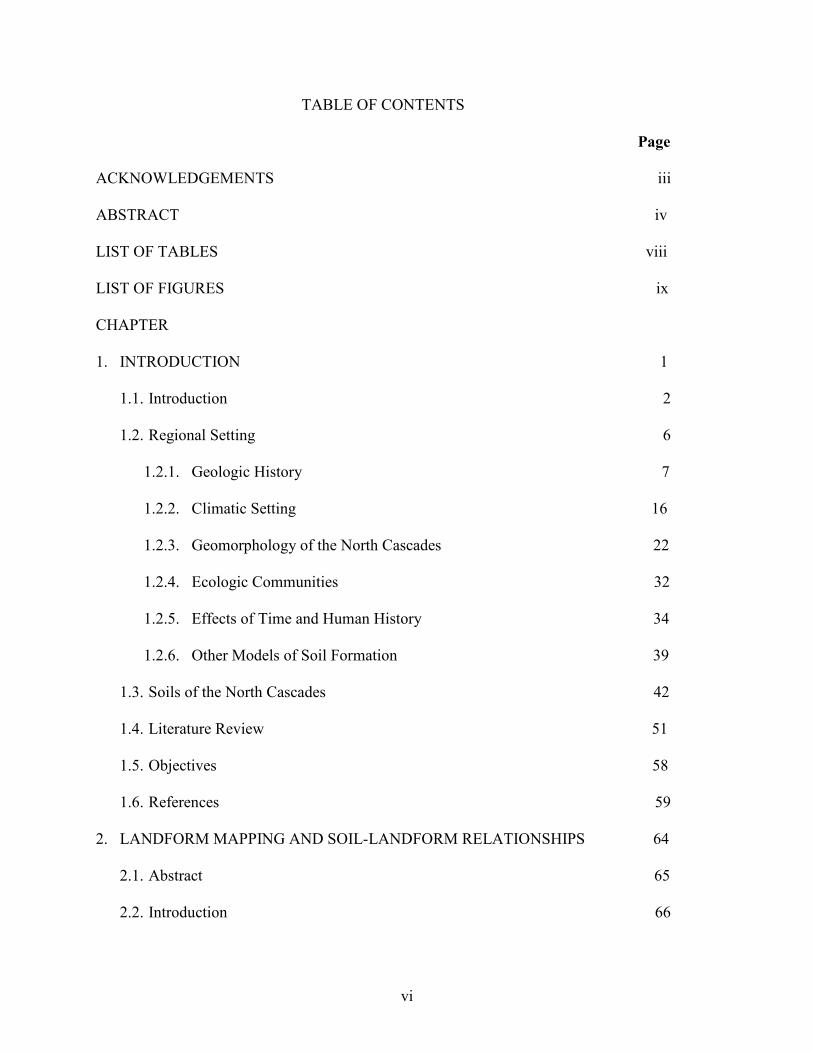
TABLE OF CONTENTS
Page
ACKNOWLEDGEMENTS iii
ABSTRACT iv
LIST OF TABLES viii
LIST OF FIGURES ix
CHAPTER
1. INTRODUCTION 1
1.1. Introduction 2
1.2. Regional Setting 6
1.2.1. Geologic History 7
1.2.2. Climatic Setting 16
1.2.3. Geomorphology of the North Cascades 22
1.2.4. Ecologic Communities 32
1.2.5. Effects of Time and Human History 34
1.2.6. Other Models of Soil Formation 39
1.3. Soils of the North Cascades 42
1.4. Literature Review 51
1.5. Objectives 58
1.6. References 59
2. LANDFORM MAPPING AND SOIL-LANDFORM RELATIONSHIPS 64
2.1. Abstract 65
2.2. Introduction 66
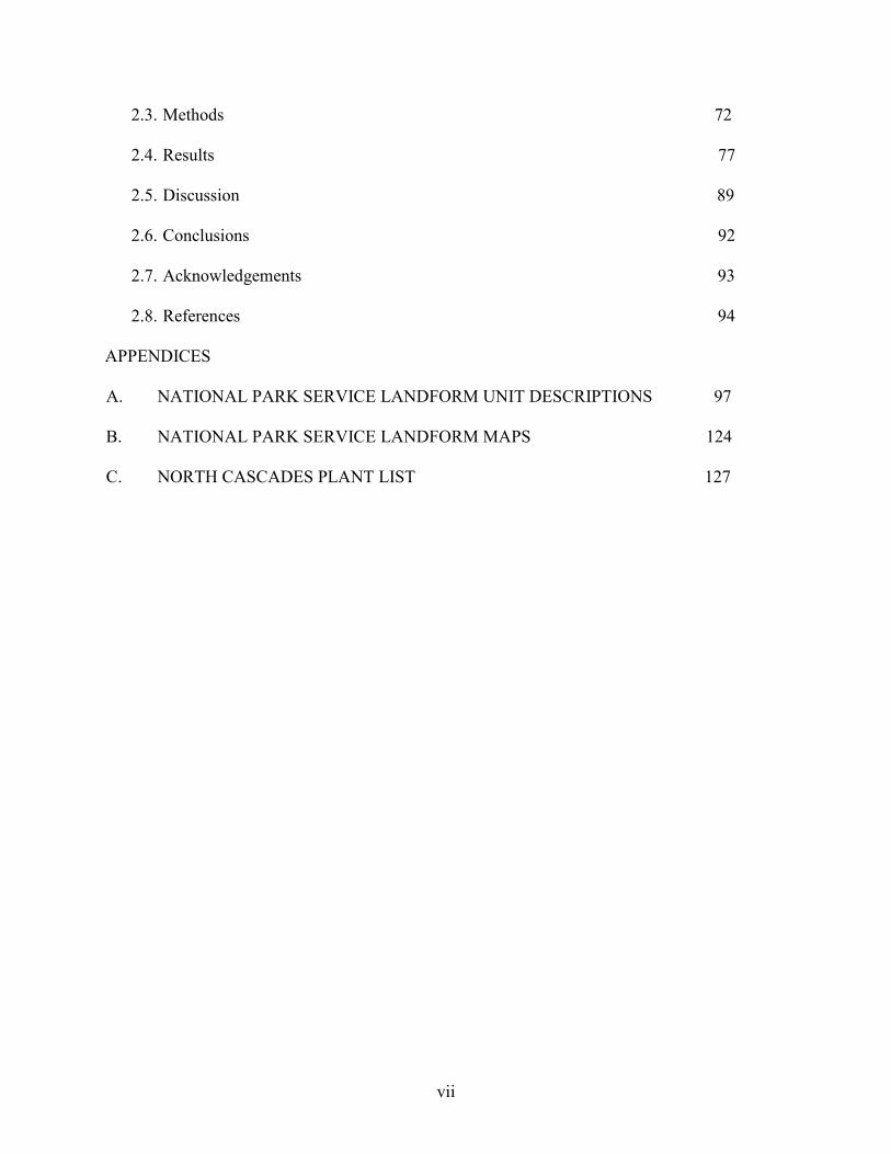
vii
2.3. Methods 72
2.4. Results 77
2.5. Discussion 89
2.6. Conclusions 92
2.7. Acknowledgements 93
2.8. References 94
APPENDICES
A. NATIONAL PARK SERVICE LANDFORM UNIT DESCRIPTIONS 97
B. NATIONAL PARK SERVICE LANDFORM MAPS 124
C. NORTH CASCADES PLANT LIST 127
viii
LIST OF TABLES
Page
1. Average Monthly Temperature and Precipitation Data 18
2. Partial Species List of Animals of the North Cascades 35
3. Partial Species List of of Fungi the North Cascades 36
4. Petrographic Microscopy Results for Samples 5 and 7 45
5. Methods for Field Identification of Landform Elements. 73
6. Comparison of Field Observations to an Existing US National Park Service 77
Landform Map
7. Results of the Recursive Partitioning and Regression Tree Analysis 78
8. Results of the Random Forest Analysis 79
9. Variable Importance as Described in the Random Forest Classification Method 80
10. Results of Watershed Mapping with Binary Decision Trees 85
11. Results of Watershed Mapping with Random Forest 85
12. Results of Regression Analyses Using Landform Elements and Terrain Attributes to 89
Model Continuous Soil Variables
ix
LIST OF FIGURES
Page
1. Map of Wilderness Areas in the United States 4
2. Soil Survey Data Currently Available in the United States 5
3. Volcanoes of the Cascade Range 8
4. Non-volcanic Peaks in the Washington Cascades 9
5. North-South tilt of Cascade Range 9
6. Geologic Domains of the North Cascades 10
7. Geologic Map of the North Cascades 11
8. Forbidden Peak 14
9. Mount Baker, a Quaternary Stratovolcano in the North Cascades 15
10. Climate Monitoring Network in the North Cascades Region 17
11. Average Monthly Temperature at the Diablo Dam Monitoring Station 19
12. Average Monthly Precipitation at the Diablo Dam Monitoring Station 20
13. Glacial and Inter-glacial Periods During the Pleistocene 21
14. Skagit River Watershed 24
15. Dams of the Skagit River Hydroelectric Project 24
16. Sub drainages within Thunder Creek Watershed 25
17. Valley Profile within McAllister Creek Valley, between Snowfield and Primus 26
Peaks
18. Valley Profile within Thunder Creek Valley, between Snowfield Peak and 26
Ragged Ridge
19. Stream Profile Graph of the West Fork of Thunder Creek 27
x
20. Stream Profile Graph of Rhode Creek 27
21. Stream Orders of Thunder Creek and its Tributaries 28
22. Eldorado Ice Cap Looking Southwest 30
23. Debris Avalanche on the West Flank of Ragged Ridge and Resulting 31
Swamp at the Mouth of Logan Creek.
24. Snow Avalanche Impact Landing; Source of Avalanches and Concave Side 32
of Snow Avalanche Impact Landing Showing Stunted Vegetation in
Foreground and Tree Throw in the Background.
25. Dates of Major Eruptions of Cascade Volcanoes. 38
26. Conceptual Model of Soil Formation Adapted for the North Cascades 41
27. Sample Locations for Mineralogical Analyses within Thunder Creek Watershed. 44
28. Scanning Electron Microscope Images of Sample 5 45
29. Scanning Electron Microscope Images of Volcanic Glass in Sample 7 46
30. Soil Orders in Thunder Creek Watershed, North Cascades National Park, 48
Washington.
31. Digital Soil Map of Thunder Creek Watershed Created by Briggs (2004). 50
32. Results of the Recursive Partitioning and Regression Tree Analysis 78
Showing Decision Rules and Output Classes of Landform Elements.
33. Results of Watershed Mapping with Binary Decision Trees 81
34. Results of Watershed Mapping with Random Forest 82
35. Qualitative Evaluation of Binary Decision Tree Results 83
36. Qualitative Evaluation of Random Forest Results 84
37. Soil Occurrence and Observed Landform Elements 86

xi
38. Podsolization Occurrence and Observed Landform Elements 86
39. Volcanic Tephra Occurrence and Observed Landform Elements 87
40. Occurrence of Redoxomorphic Features and observed landform Elements 87
41. Distribution of Soil Orders with Respect to Landform Elements 88

CHAPTER ONE - INTRODUCTION

2
1.1 Introduction
In this thesis, I employed digital methods to map landforms and soils in a wilderness.
Soils are the living skin that covers the surface of the terrestrial earth. Landforms are dynamic
entities created by the exposure of the earth’s surface to erosional forces, including water, ice,
gravity, and wind. The effects of weathering agents across a landscape produce unique spatial
patterns. These individual facets often have relatively homogeneous soil characteristics.
In 1964, the Wilderness Act was passed, designating 54 areas (9.1 million acres) in 13
states as Wilderness. In May of 2008, President George W. Bush created the Wild Sky
Wilderness in eastern Snohomish County, Washington, the newest wilderness in the country.
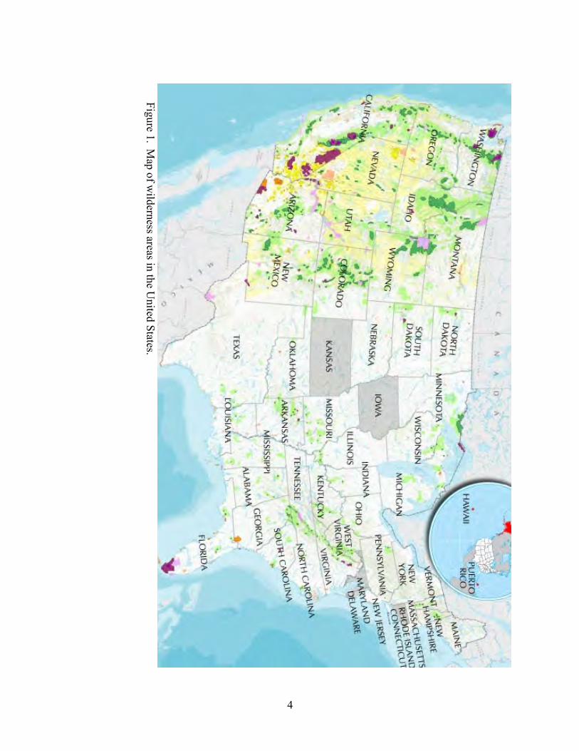
Currently in the United States 434 km2 are designated as federally protected wilderness, covering
approximately 5% of the nation (Figure 1). In Washington, wilderness covers 1,790 hectares and
covers over 10% of the state. The National Park Service (NPS, 39% of the state) and Forest
Service (USFS, 60% of the state) manage the majority of wilderness areas in Washington. The
Fish and Wildlife Service and the Bureau of Land Management also managed smaller wilderness
areas (<1% combined). The Wilderness Act defines wilderness in Section 2(c) as follows, “A
wilderness, in contrast with those areas where man and his own works dominate the landscape, is
hereby recognized as an area where the earth and its community of life are untrammeled by man,
where man himself is a visitor who does not remain. An area of wilderness is further defined to
mean in this Act an area of undeveloped Federal land retaining its primeval character and
influence, without permanent improvements or human habitation, which is protected and
managed so as to preserve its natural conditions and which (1) generally appears to have been
affected primarily by the forces of nature, with the imprint of man's work substantially
unnoticeable; (2) has outstanding opportunities for solitude or a primitive and unconfined type of

3
recreation; (3) has at least five thousand acres of land or is of sufficient size as to make
practicable its preservation and use in an unimpaired condition; and (4) may also contain
ecological, geological, or other features of scientific, educational, scenic, or historical value.”
A desire exists to complete soil mapping of the United States. Over a century a work by
the National Cooperative Soil Survey has yet to provide soil data for all of the conterminous
United States (Figure 2). Of the approximately 8,080,400 km2 in the lower 48 States, 649,000
km2 (8.03 %) lack soil data. The US Forest Service and National Park Service (NPS) manage an
approximate total of 342,000 km2 of these unmapped areas. This amounts to 53.78 % of the
unmapped areas and 4.24 % of the lower 48 States, with the majority of these areas occurring in
mountainous regions of the Western United States. These statistics are even more dramatic if the
numerous wildernesses of Alaska are included.
To date, soil mapping efforts in the United States have not focused on mountainous
wilderness areas. Areas without existing soil maps (Figure 2) are closely correlated with
wilderness areas (Figure 1), especially in the Western United States. Remote and inaccessible
regions require less management actions and hence, are frequently ignored from traditional soil
surveys. Vehicle access is restricted in wilderness areas, therefore, horse packing and hiking are
the most common forms of transportation. Wilderness lands have been traditionally excluded
from soil and landform inventories, due to the logistical challenge posed; however, wilderness
soils are important to the study of soil classification and mapping because they are generally not
altered by human activity. Research from these areas fills in gaps where soils data are lacking,
providing information for scientifically based management of public resources and increased
knowledge of soil-landform relationships in remote, mountainous areas.
4
Figure 1
. Map of w
ildern
ess areas in th
e United
States.
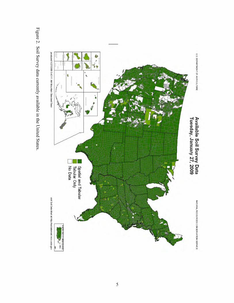
5
Figure 2
. Soil S
urvey data cu
rrently
availab
le in th
e United
States.

6
Computing power, remote sensing and geographic information systems have provided
new technologies to quantify the shape of the earth’s surface. Satellites are currently observing
the topography of and the reflectance of energy from the earth. These tools have been applied to
gather data from wilderness areas. Digital landform and soil mapping provide information
regarding the shape of the land surface and soil properties through a cost effective means.
Data from digital landform and soil mapping (DLM and DSM, respectively) can be used
to promote scientifically based management of public resources. The data available through
DLM and DSM serves as baseline data for other investigations within these areas (i.e., wildlife
conservation, habitat protection, suitability analyses). Soils also play an essential role in the
storage of carbon on earth. Soil mapping provides information related to global biogeochemical
cycles and climate change. By monitoring landform and soil distribution, one can address issues
regarding the way an environment responds to ecosystem changes like fires, landslides,
avalanches, and logging.
The research presented here builds on the work of Rodgers (2000), Ufnar (2004), Briggs
(2004) and Meirik (2008). I employed digital methods to map landforms and soils in a
wilderness in the Pacific Northwest (PNW). I described and classified soils and landforms
during 2007 and 2008 in the North Cascades National Park. This required spending extended
time in the Stephen T. Mather Wilderness, traveling to remote locations in order to observe land
surface characteristics, soil profiles, and plant communities. The rugged mountainous nature of
this region requires technical mountaineering abilities to travel at will across landscapes.
1.2 Regional Setting
This is included to provide background information about the North Cascades (NOCA)
region using the soil factor equation proposed by Jenny (1941). This model states that a given
7
soil is a function of parent material, topography, climate, organisms, and time. Geology, climate,
geomorphology, ecology, and human history of NOCA will be discussed to further acquaint the
reader with the NOCA. Each of these factors will be explored with respect to soil genesis in the
region. Then, the SCORPAN model (McBratney et al., 2003) will be commented on with
regards to DSM. Finally, a detailed examination of the regional soils will be provided.
1.2.1 Geologic History
The Cascade Range is the portion of the North American Cordillera between the Sierra
Nevada in California and the Costal Ranges of British Columbia (Tabor and Haugerud, 1999).
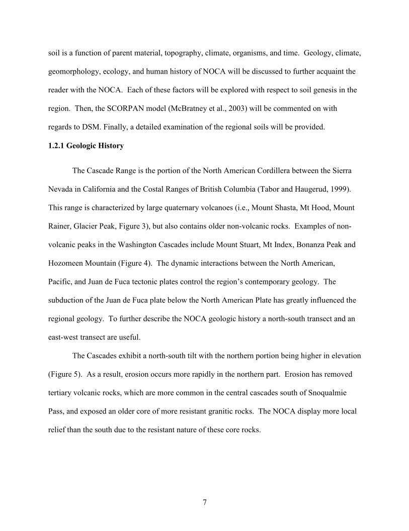
This range is characterized by large quaternary volcanoes (i.e., Mount Shasta, Mt Hood, Mount
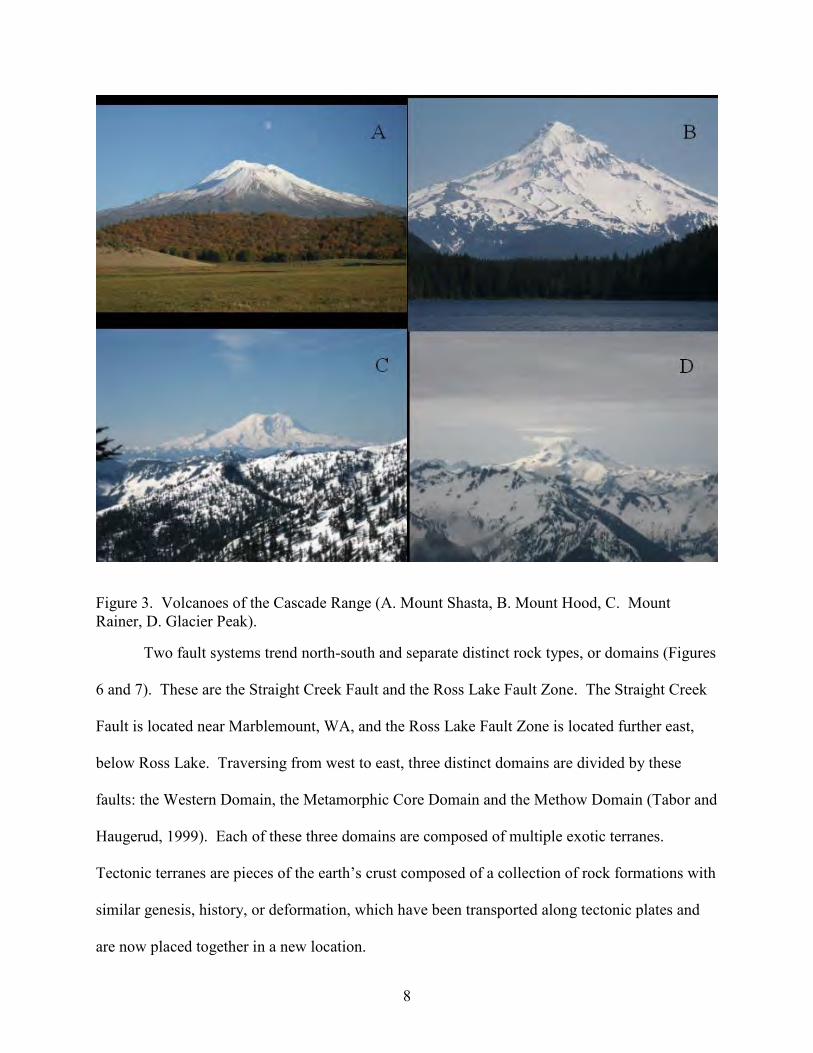
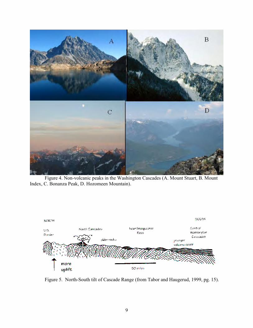
Rainer, Glacier Peak, Figure 3), but also contains older non-volcanic rocks. Examples of non-
volcanic peaks in the Washington Cascades include Mount Stuart, Mt Index, Bonanza Peak and
Hozomeen Mountain (Figure 4). The dynamic interactions between the North American,
Pacific, and Juan de Fuca tectonic plates control the region’s contemporary geology. The
subduction of the Juan de Fuca plate below the North American Plate has greatly influenced the
regional geology. To further describe the NOCA geologic history a north-south transect and an
east-west transect are useful.
The Cascades exhibit a north-south tilt with the northern portion being higher in elevation
(Figure 5). As a result, erosion occurs more rapidly in the northern part. Erosion has removed
tertiary volcanic rocks, which are more common in the central cascades south of Snoqualmie
Pass, and exposed an older core of more resistant granitic rocks. The NOCA display more local
relief than the south due to the resistant nature of these core rocks.
8
Figure 3. Volcanoes of the Cascade Range (A. Mount Shasta, B. Mount Hood, C. Mount
Rainer, D. Glacier Peak).
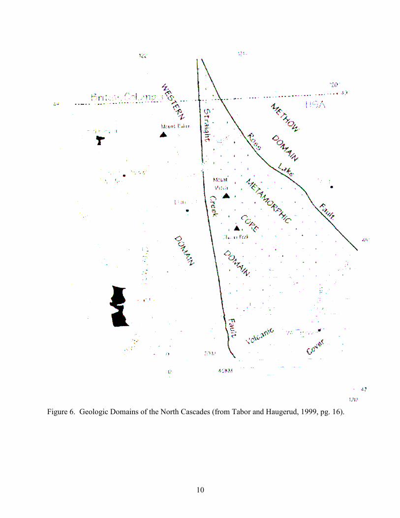
Two fault systems trend north-south and separate distinct rock types, or domains (Figures
6 and 7). These are the Straight Creek Fault and the Ross Lake Fault Zone. The Straight Creek
Fault is located near Marblemount, WA, and the Ross Lake Fault Zone is located further east,
below Ross Lake. Traversing from west to east, three distinct domains are divided by these
faults: the Western Domain, the Metamorphic Core Domain and the Methow Domain (Tabor and
Haugerud, 1999). Each of these three domains are composed of multiple exotic terranes.
Tectonic terranes are pieces of the earth’s crust composed of a collection of rock formations with
similar genesis, history, or deformation, which have been transported along tectonic plates and
are now placed together in a new location.
9
Figure 4. Non-volcanic peaks in the Washington Cascades (A. Mount Stuart, B. Mount
Index, C. Bonanza Peak, D. Hozomeen Mountain).
Figure 5. North-South tilt of Cascade Range (from Tabor and Haugerud, 1999, pg. 15).
10
Figure 6. Geologic Domains of the North Cascades (from Tabor and Haugerud, 1999, pg. 16).

11
Figure 7
. Geologic M
ap of th
e North
Cascad
es (from Tabor an
d Haugeru
d, 1
999).
12
In the NOCA, the Western Domain is composed of the Nooksack Terrane, the Chilliwack
River Terrane, the Bell Pass Melange and the Easton Terrane. These terranes are listed from
lowest to highest in a pile produced by thrust faults between each terrane. However, the
youngest terrane (Nooksack) is at the bottom of this pile. This pattern was produced when
terranes collided with the North American plate and formed an accretionary prism of sediments
not subducted beneath the continent. This stack of sediment grows through accumulation of
terranes traveling with plate motions and colliding with continents, and subsequently being
positioned on land through thrust faulting. Dominant rock types include sedimentary and
volcanic rocks that were produced close to the earth’s surface. Although these rocks have
undergone complex folding and faulting, sedimentary structures and fossils remain intact.
To the East, the straight creek fault divides the Western Domain from the Metamorphic
Core Domain. This domain is composed of four terranes; the Chelan Mountains Terrane, the
Nason Terrane, the Swakane Terrane and the Little Jack Terrane. The major rock type in this
domain is metamorphic rocks. The birthplaces of these rocks have distinctly different
characteristics. Ocean sediments, volcanic arc sediments and marine sediments derived from
continental crusts are the three main precursors to the metamorphic rocks observed today. TCW
is located with in this terrane, specifically within the Chelan Mountains Terrane.
Finally, further to the East one encounters the Methow Domain, composed of the
Methow and Hozomeen terranes. This domain is composed largely of sedimentary and volcanic
rocks, with a less complex history of deformation. This domain is located east of the Ross Lake
Fault Zone. Many of the rocks in the region were produced when unmetamorphosed sandstones
and shales were deposited in submarine fans at the edge of the continent. In general this domain
exhibits more order in the bedding sequences and a more predictable behavior.
13
The numerous unique terranes of the various domains assembled over Western
Washington towards the end of the Cretaceous Period (approximately 90 million years before
present, ybp). The majority of the rock in the Metamorphic Core Domain was added to the
margin of North America in a thrust stack formed in an accretionary prism. These rocks were
deep enough in the pile to receive sufficient heat and pressure to drive deformation. In addition,
magma produced by subduction of the Juan de Fuca Plate, fueled plutonic intrusions. These two
mechanisms are the main causes of recrystallization, which occurred from approximately from
90 to 65 million ybp. In addition, foliations in these rocks provide evidence of squeezing,
stretching and deformation as the recrystallization was occurring. Another period of
metamorphism occurred in the Eocene (45 million ybp), with the return of volcanism and the
awakening of the Cascade Volcanic Arc.
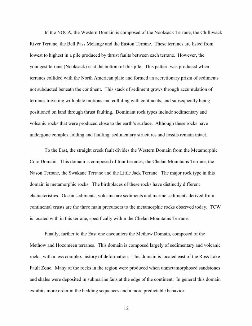
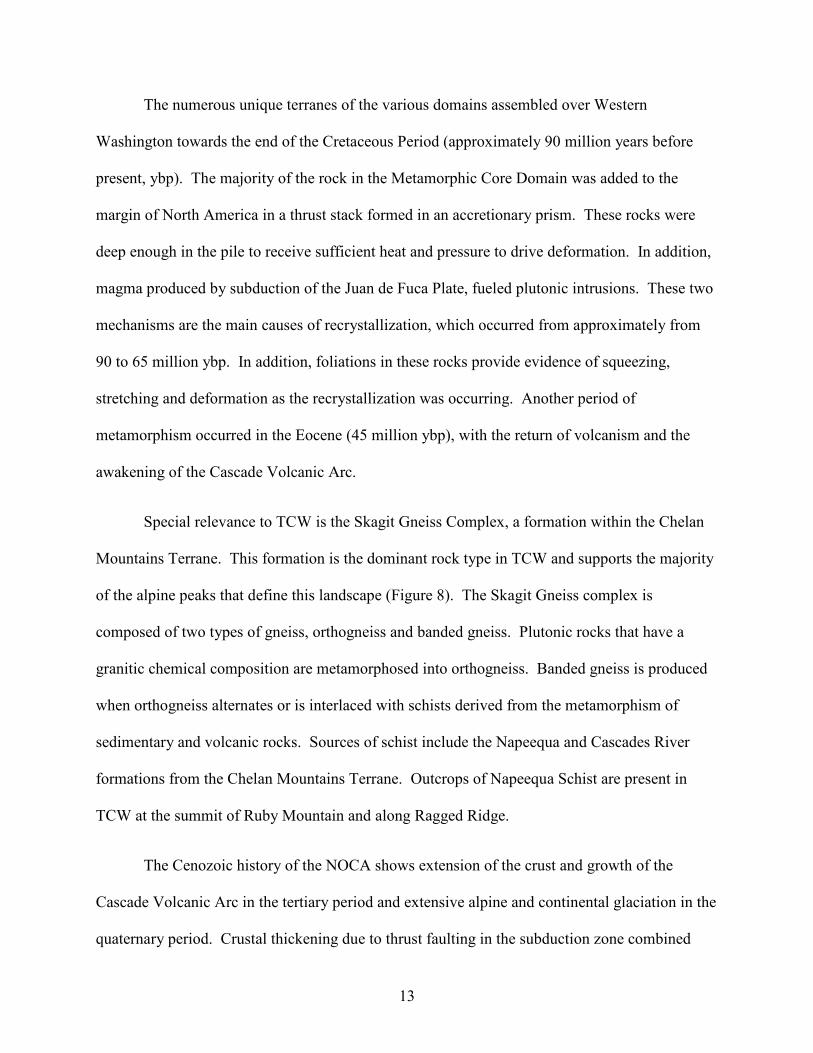
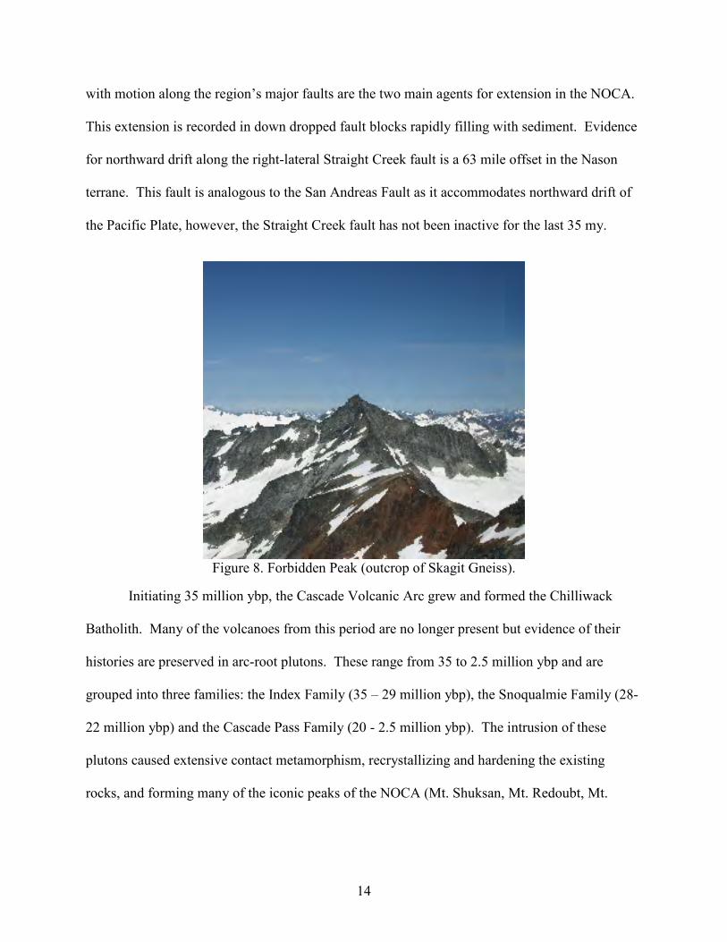
Special relevance to TCW is the Skagit Gneiss Complex, a formation within the Chelan
Mountains Terrane. This formation is the dominant rock type in TCW and supports the majority
of the alpine peaks that define this landscape (Figure 8). The Skagit Gneiss complex is
composed of two types of gneiss, orthogneiss and banded gneiss. Plutonic rocks that have a
granitic chemical composition are metamorphosed into orthogneiss. Banded gneiss is produced
when orthogneiss alternates or is interlaced with schists derived from the metamorphism of
sedimentary and volcanic rocks. Sources of schist include the Napeequa and Cascades River
formations from the Chelan Mountains Terrane. Outcrops of Napeequa Schist are present in
TCW at the summit of Ruby Mountain and along Ragged Ridge.
The Cenozoic history of the NOCA shows extension of the crust and growth of the
Cascade Volcanic Arc in the tertiary period and extensive alpine and continental glaciation in the
quaternary period. Crustal thickening due to thrust faulting in the subduction zone combined
14
with motion along the region’s major faults are the two main agents for extension in the NOCA.
This extension is recorded in down dropped fault blocks rapidly filling with sediment. Evidence
for northward drift along the right-lateral Straight Creek fault is a 63 mile offset in the Nason
terrane. This fault is analogous to the San Andreas Fault as it accommodates northward drift of
the Pacific Plate, however, the Straight Creek fault has not been inactive for the last 35 my.
Figure 8. Forbidden Peak (outcrop of Skagit Gneiss).
Initiating 35 million ybp, the Cascade Volcanic Arc grew and formed the Chilliwack
Batholith. Many of the volcanoes from this period are no longer present but evidence of their
histories are preserved in arc-root plutons. These range from 35 to 2.5 million ybp and are
grouped into three families: the Index Family (35 – 29 million ybp), the Snoqualmie Family (28-
22 million ybp) and the Cascade Pass Family (20 - 2.5 million ybp). The intrusion of these
plutons caused extensive contact metamorphism, recrystallizing and hardening the existing
rocks, and forming many of the iconic peaks of the NOCA (Mt. Shuksan, Mt. Redoubt, Mt.
15
Challenger and Hozomeen Mt.). Evidence of these old volcanoes are seen in the Kulshan and
Hannegan Calderas, the Big Bosom Buttes, Pioneer Ridge and Mt. Rham.
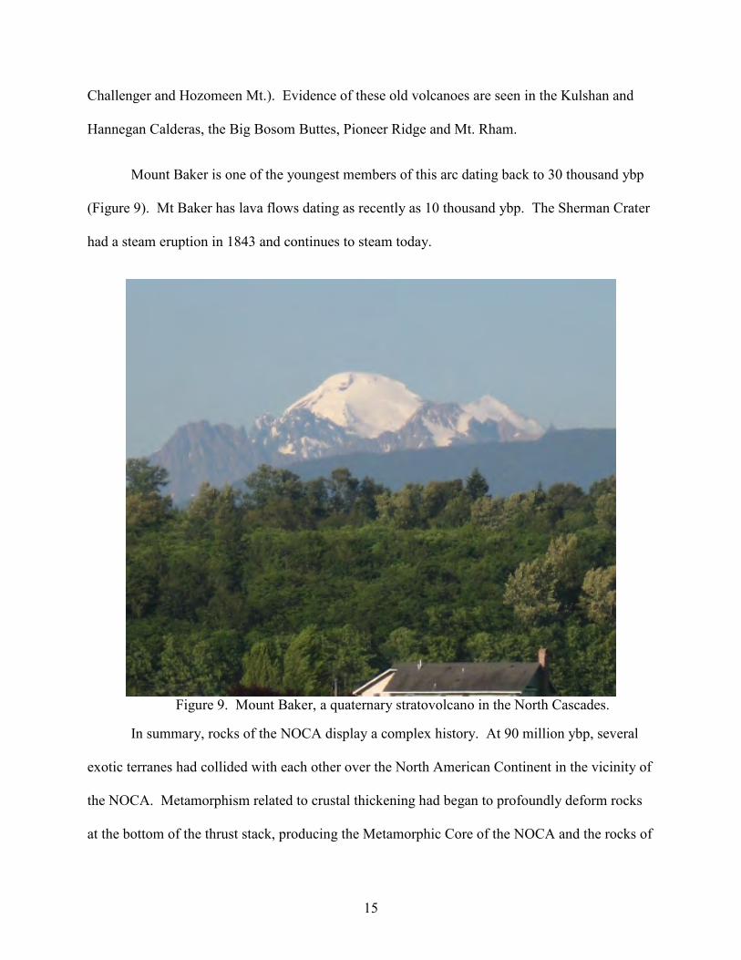
Mount Baker is one of the youngest members of this arc dating back to 30 thousand ybp
(Figure 9). Mt Baker has lava flows dating as recently as 10 thousand ybp. The Sherman Crater
had a steam eruption in 1843 and continues to steam today.
Figure 9. Mount Baker, a quaternary stratovolcano in the North Cascades.
In summary, rocks of the NOCA display a complex history. At 90 million ybp, several
exotic terranes had collided with each other over the North American Continent in the vicinity of
the NOCA. Metamorphism related to crustal thickening had began to profoundly deform rocks
at the bottom of the thrust stack, producing the Metamorphic Core of the NOCA and the rocks of

16
the Skagit Gneiss Complex, which dominate TCW. During the Eocene plate motions changed to
produce local extension and northward drift along the Straight Creek fault. However
metamorphism resumed approximately 45 million ybp. By 35 million ybp, plate motions had
greatly decreased and the Cascade Volcanic Arc formed the Chilliwack Batholith and associated
volcanic vents. Pleistocene glaciations have profoundly effected the region through six separate
advances in the last 2 my. Only recently (30 thousand ybp) in this complex history have the
quaternary volcanoes grown that define the Cascade Range.
1.2.2 Climatic Setting
The PNW is characterized by a humid temperate climate with topography and proximity
to the ocean being the major controls on regional climate. Maritime influence is prominent as
tidewater is as close as 80 km to the heart of the Cascade Range. Proximity to the Northern
Pacific Ocean produces significant moisture as precipitation and snow. The corridors provided
by the Skagit and Fraser River Valleys allow marine air to penetrate deep into the mountainous
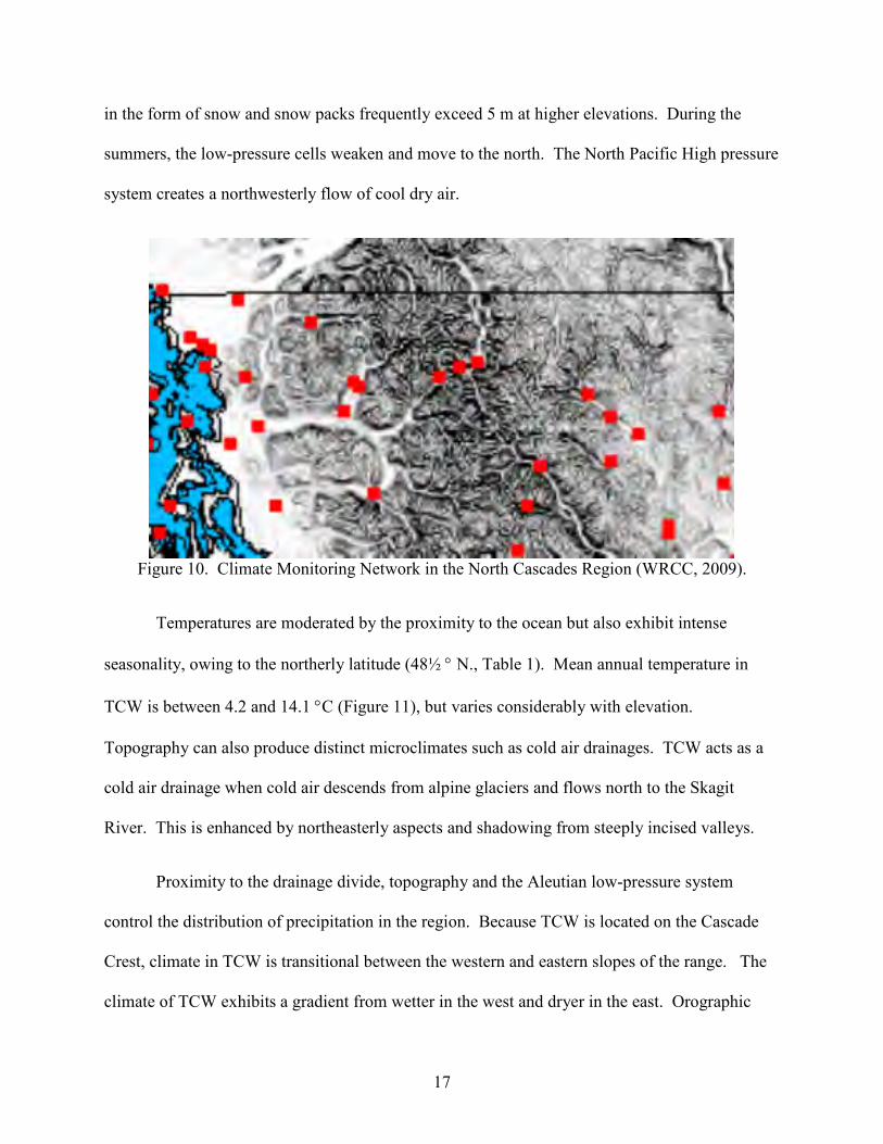
interior. Mean annual precipitation is over 190 cm in TCW. An extensive network of
monitoring stations is in place around the area (Figure 10), and some have been collecting data
for almost a century.
In the NOCA, precipitation falls mostly in the winter, leaving relatively warm and dry
summers. Two semi-permanent pressure systems control local climate (Beckey, 1995; Beckey,
2003). In the summer, the North Pacific High pressure system migrates over the NOCA. This
clockwise circulation brings cool marine air south and east to the Cascades. A rainy season is
produced in the late fall and winter by the Aleutian low-pressure system. This counterclockwise
circulation brings a southwesterly flow of cool marine air. The majority of the precipitation falls
17
in the form of snow and snow packs frequently exceed 5 m at higher elevations. During the
summers, the low-pressure cells weaken and move to the north. The North Pacific High pressure
system creates a northwesterly flow of cool dry air.
Figure 10. Climate Monitoring Network in the North Cascades Region (WRCC, 2009).
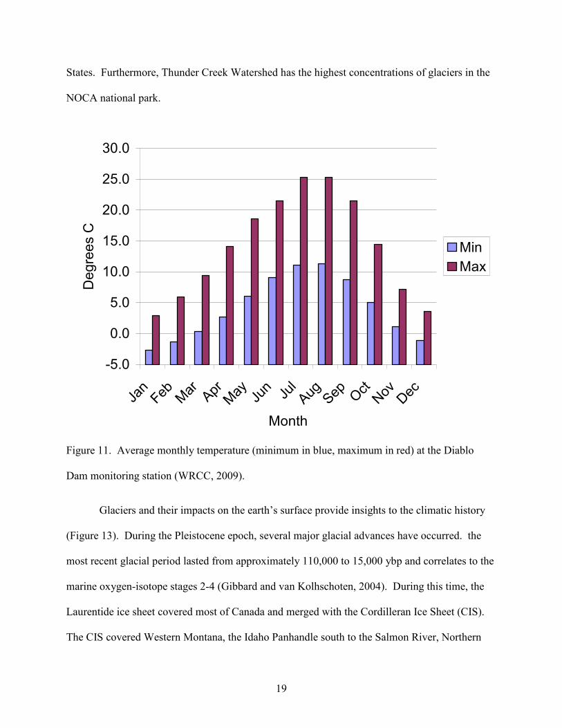
Temperatures are moderated by the proximity to the ocean but also exhibit intense
seasonality, owing to the northerly latitude (48½ ° N., Table 1). Mean annual temperature in
TCW is between 4.2 and 14.1 °C (Figure 11), but varies considerably with elevation.
Topography can also produce distinct microclimates such as cold air drainages. TCW acts as a
cold air drainage when cold air descends from alpine glaciers and flows north to the Skagit
River. This is enhanced by northeasterly aspects and shadowing from steeply incised valleys.
Proximity to the drainage divide, topography and the Aleutian low-pressure system
control the distribution of precipitation in the region. Because TCW is located on the Cascade
Crest, climate in TCW is transitional between the western and eastern slopes of the range. The
climate of TCW exhibits a gradient from wetter in the west and dryer in the east. Orographic
18
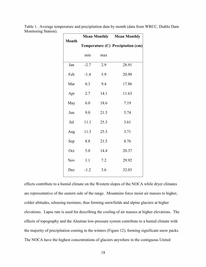
Table 1. Average temperature and precipitation data by month (data from WRCC, Diablo Dam
Monitoring Station).
Month
Mean Monthly
Temperature (C)
Mean Monthly
Preciptation (cm)
min max
Jan -2.7 2.9 28.91
Feb -1.4 5.9 20.90
Mar 0.3 9.4 17.86
Apr 2.7 14.1 11.63
May 6.0 18.6 7.19
Jun 9.0 21.5 5.74
Jul 11.1 25.3 3.61
Aug 11.3 25.3 3.71
Sep 8.8 21.5 8.76
Oct 5.0 14.4 20.37
Nov 1.1 7.2 29.92
Dec -1.2 3.6 32.03
effects contribute to a humid climate on the Western slopes of the NOCA while dryer climates
are representative of the eastern side of the range. Mountains force moist air masses to higher,
colder altitudes, releasing moisture, thus forming snowfields and alpine glaciers at higher
elevations. Lapse rate is used for describing the cooling of air masses at higher elevations. The
effects of topography and the Aleutian low-pressure system contribute to a humid climate with
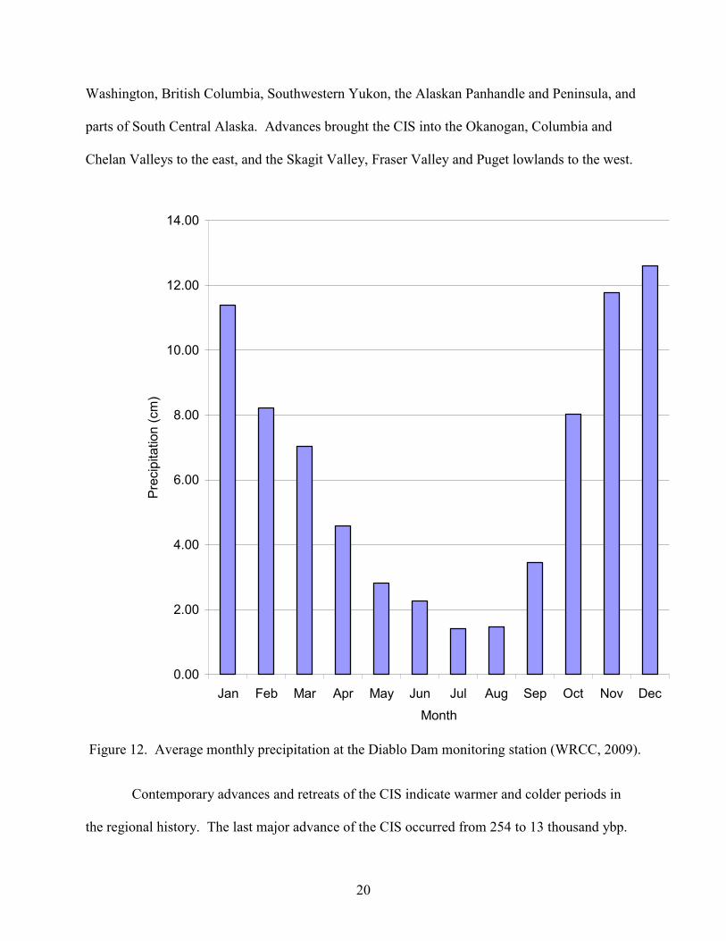
the majority of precipitation coming in the winters (Figure 12), forming significant snow packs.
The NOCA have the highest concentrations of glaciers anywhere in the contiguous United
19
States. Furthermore, Thunder Creek Watershed has the highest concentrations of glaciers in the
NOCA national park.
-5.0
0.0
5.0
10.0
15.0
20.0
25.0
30.0
JanFebMar
Apr
May Ju
nJulAug
Sep O
ctNov
Dec
Month
Degrees C
Min
Max
Figure 11. Average monthly temperature (minimum in blue, maximum in red) at the Diablo
Dam monitoring station (WRCC, 2009).
Glaciers and their impacts on the earth’s surface provide insights to the climatic history
(Figure 13). During the Pleistocene epoch, several major glacial advances have occurred. the
most recent glacial period lasted from approximately 110,000 to 15,000 ybp and correlates to the
marine oxygen-isotope stages 2-4 (Gibbard and van Kolhschoten, 2004). During this time, the
Laurentide ice sheet covered most of Canada and merged with the Cordilleran Ice Sheet (CIS).
The CIS covered Western Montana, the Idaho Panhandle south to the Salmon River, Northern
20
Washington, British Columbia, Southwestern Yukon, the Alaskan Panhandle and Peninsula, and
parts of South Central Alaska. Advances brought the CIS into the Okanogan, Columbia and
Chelan Valleys to the east, and the Skagit Valley, Fraser Valley and Puget lowlands to the west.
0.00
2.00
4.00
6.00
8.00
10.00
12.00
14.00
Jan Feb Mar Apr May Jun Jul Aug Sep Oct Nov Dec
Month
Precipitation (cm)
Figure 12. Average monthly precipitation at the Diablo Dam monitoring station (WRCC, 2009).
Contemporary advances and retreats of the CIS indicate warmer and colder periods in
the regional history. The last major advance of the CIS occurred from 254 to 13 thousand ybp.

21
Glacier Peak tephra indicates retreat of the CIS by as much as 80 km by 12,000 ybp (Beckey,
2003). Ice began its retreat before the Missoula Floods and formation of the channeled scablands
(Allen et al., 1986). The Majority of the CIS in the NOCA had melted by roughly 12,750 ybp.
A smaller advance was recorded approximately 7,000 ybp. The Little Ice Age (LIA)
marked a period of global cooling and advances of glaciers in the Pacific Northwest, European
Alps and Himalayas spanning the 13th to 20
th century. The LIA peaked in the mid 18
th century
and again in the late 19th to early 20
th centuries.
Figure 13. Glacial and inter-glacial periods during the Pleistocene.
(http://en.wikipedia.org/wiki/File:Atmospheric_CO2_with_glaciers_cycles.gif)
More recently glaciers have generally been receding, with an exception occurring in the
1950’s (Beckey, 2003). Glaciers on Mount Baker were growing in 1975 (Pelto and Riedel,
2001). From 1977 to 1994 NOCA glaciers exhibited a negative mass balance and were
22
retreating (Pelto and Riedel, 2001). From 1995 to 2000 annual mass balance trends are slightly
positive (0.15 m per year) for 14 glaciers monitored by the NOCA NP, USGS, and the North
Cascades Glacier Climate Project (NCGCP, Pelto and Riedel, 2001).
1.2.3 Geomorphology of the North Cascades
Steep, mountainous topography is characteristic of the NOCA. The recent actions of
gravity, water, and ice have sculpted the valleys and peaks that now characterize the topography
of the landscape. Combinations of rivers, glaciers, mass movements and avalanches produced
unique landforms with NOCA. Humid climate with an abundance of precipitation feeds glaciers
and controls the regional hydrology. Alpine and continental glaciations have major impacts on
the nature of these landscapes. Mass movements are common features in this region due to the
steep topography. The effects of water, ice and gravity produce unique depositional landsurfaces
governed by the specific mechanisms of erosion. The topography of this watershed is diverse in
landforms, owing to the multitude of forces that have built and are leveling the mountainous
landscape.
Geomorphology has been studied in the context of process-response systems (Conacher
and Dalrymple, 1977; Ritter et al., 2002). In these systems, a given process is responsible for
producing landforms (the response). In the NOCA, water, ice and gravity are the principle
agents of erosion of the geologic substrate. The ubiquitous presence of water has carved deep
valleys and leaves stunning waterfalls. The broad U-shaped valleys are indicative of glacial
activity. Glaciers also are responsible for the formation of cirques, arêtes, and moraines that are
present in the watershed. Gravity is responsible for the mass movements that erode the valley
23
walls. Numerous landslides are evident throughout the watershed. To understand the landforms
of TCW and the NOCA, I will discuss the major processes and how they shape the land surface.
Regional hydrology drains into the Pacific Ocean through the Skagit River to the west,
the Columbia River to the east and the Fraser River to the north in British Columbia. Principle
drainage divides are the Pacific Crest, trending north-south and dividing the Skagit and
Columbia Rivers and the North Cascade Crest, trending east-west and dividing the Skagit and
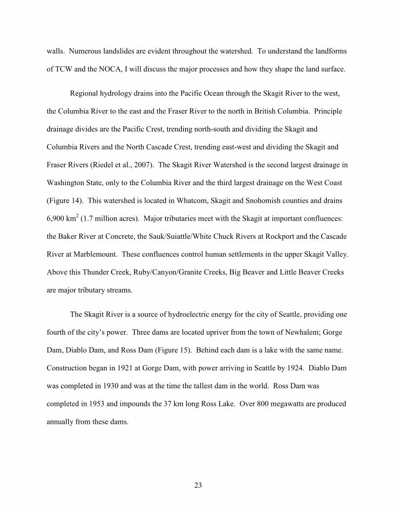
Fraser Rivers (Riedel et al., 2007). The Skagit River Watershed is the second largest drainage in
Washington State, only to the Columbia River and the third largest drainage on the West Coast
(Figure 14). This watershed is located in Whatcom, Skagit and Snohomish counties and drains
6,900 km2 (1.7 million acres). Major tributaries meet with the Skagit at important confluences:
the Baker River at Concrete, the Sauk/Suiattle/White Chuck Rivers at Rockport and the Cascade
River at Marblemount. These confluences control human settlements in the upper Skagit Valley.
Above this Thunder Creek, Ruby/Canyon/Granite Creeks, Big Beaver and Little Beaver Creeks
are major tributary streams.
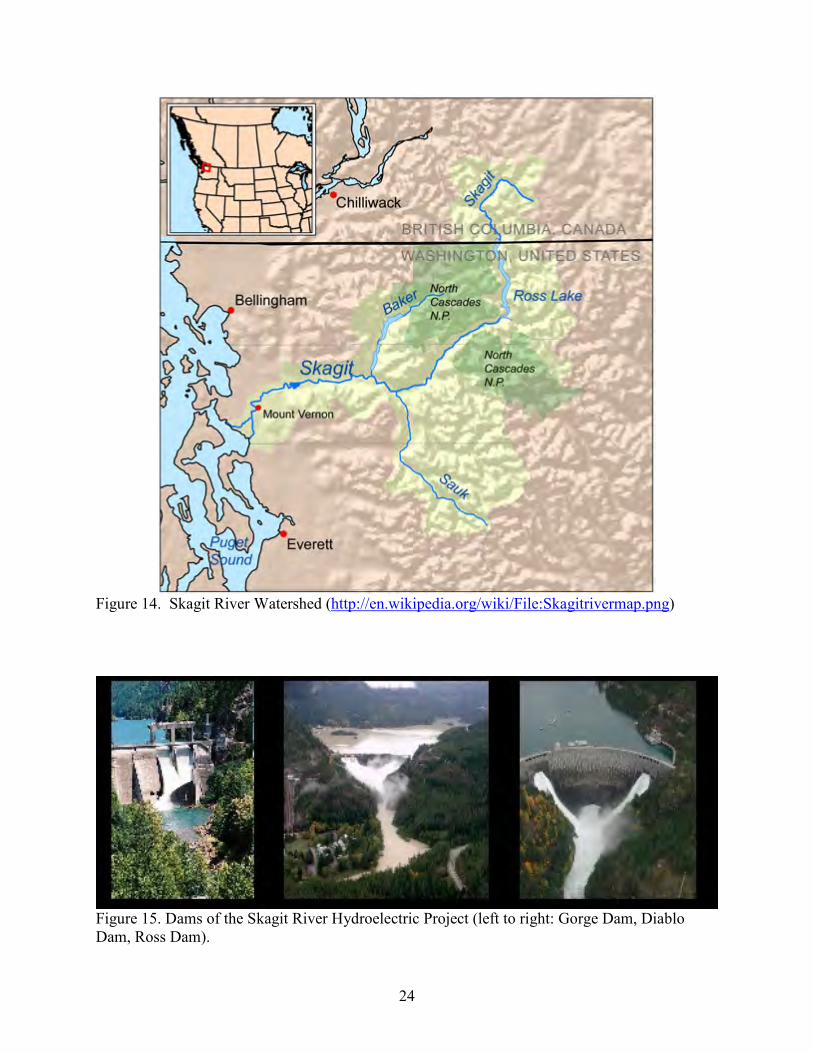
The Skagit River is a source of hydroelectric energy for the city of Seattle, providing one
fourth of the city’s power. Three dams are located upriver from the town of Newhalem; Gorge
Dam, Diablo Dam, and Ross Dam (Figure 15). Behind each dam is a lake with the same name.
Construction began in 1921 at Gorge Dam, with power arriving in Seattle by 1924. Diablo Dam
was completed in 1930 and was at the time the tallest dam in the world. Ross Dam was
completed in 1953 and impounds the 37 km long Ross Lake. Over 800 megawatts are produced
annually from these dams.
24
Figure 14. Skagit River Watershed (http://en.wikipedia.org/wiki/File:Skagitrivermap.png)
Figure 15. Dams of the Skagit River Hydroelectric Project (left to right: Gorge Dam, Diablo
Dam, Ross Dam).
25
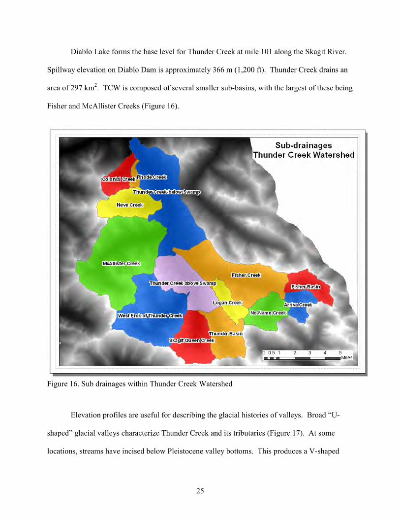
Diablo Lake forms the base level for Thunder Creek at mile 101 along the Skagit River.
Spillway elevation on Diablo Dam is approximately 366 m (1,200 ft). Thunder Creek drains an
area of 297 km2. TCW is composed of several smaller sub-basins, with the largest of these being
Fisher and McAllister Creeks (Figure 16).
Figure 16. Sub drainages within Thunder Creek Watershed
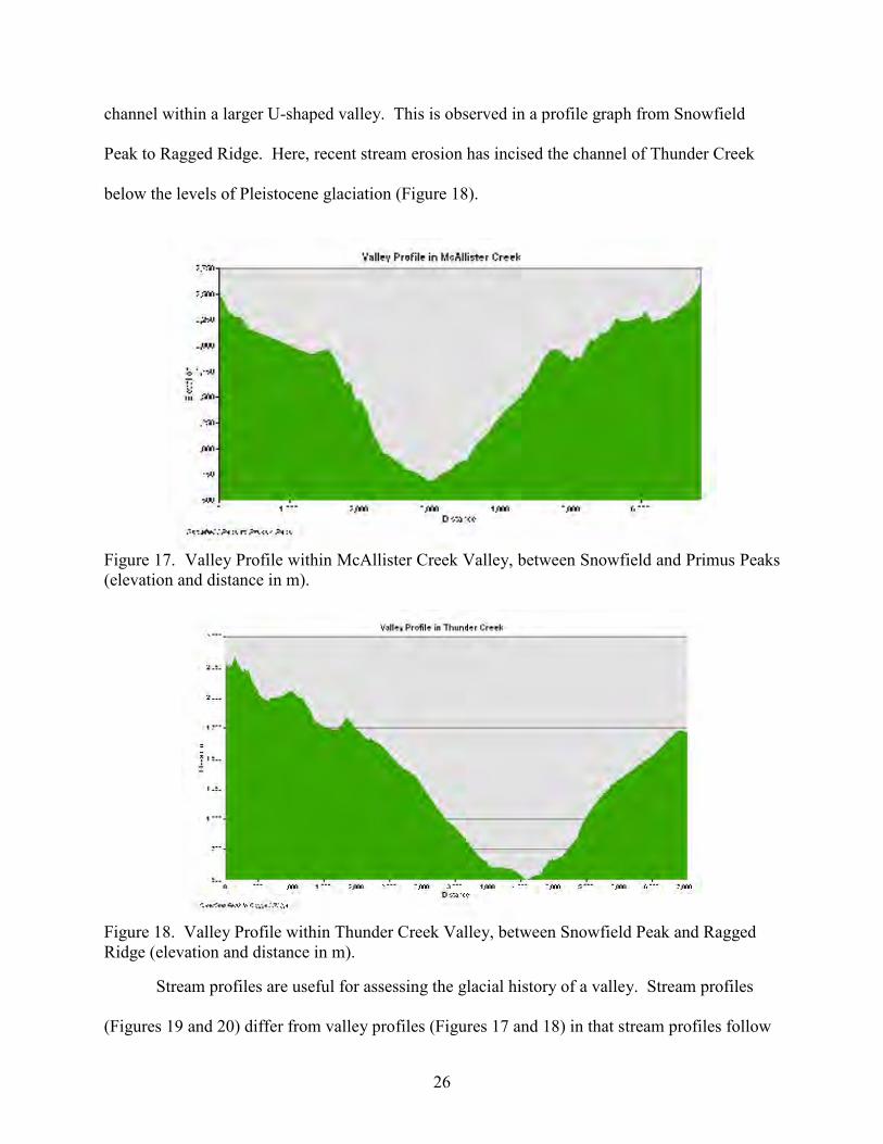
Elevation profiles are useful for describing the glacial histories of valleys. Broad “U-
shaped” glacial valleys characterize Thunder Creek and its tributaries (Figure 17). At some
locations, streams have incised below Pleistocene valley bottoms. This produces a V-shaped
26
channel within a larger U-shaped valley. This is observed in a profile graph from Snowfield
Peak to Ragged Ridge. Here, recent stream erosion has incised the channel of Thunder Creek
below the levels of Pleistocene glaciation (Figure 18).
Figure 17. Valley Profile within McAllister Creek Valley, between Snowfield and Primus Peaks
(elevation and distance in m).
Figure 18. Valley Profile within Thunder Creek Valley, between Snowfield Peak and Ragged
Ridge (elevation and distance in m).
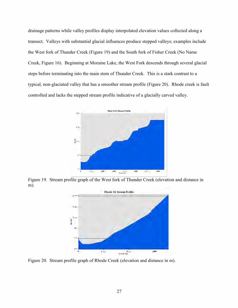
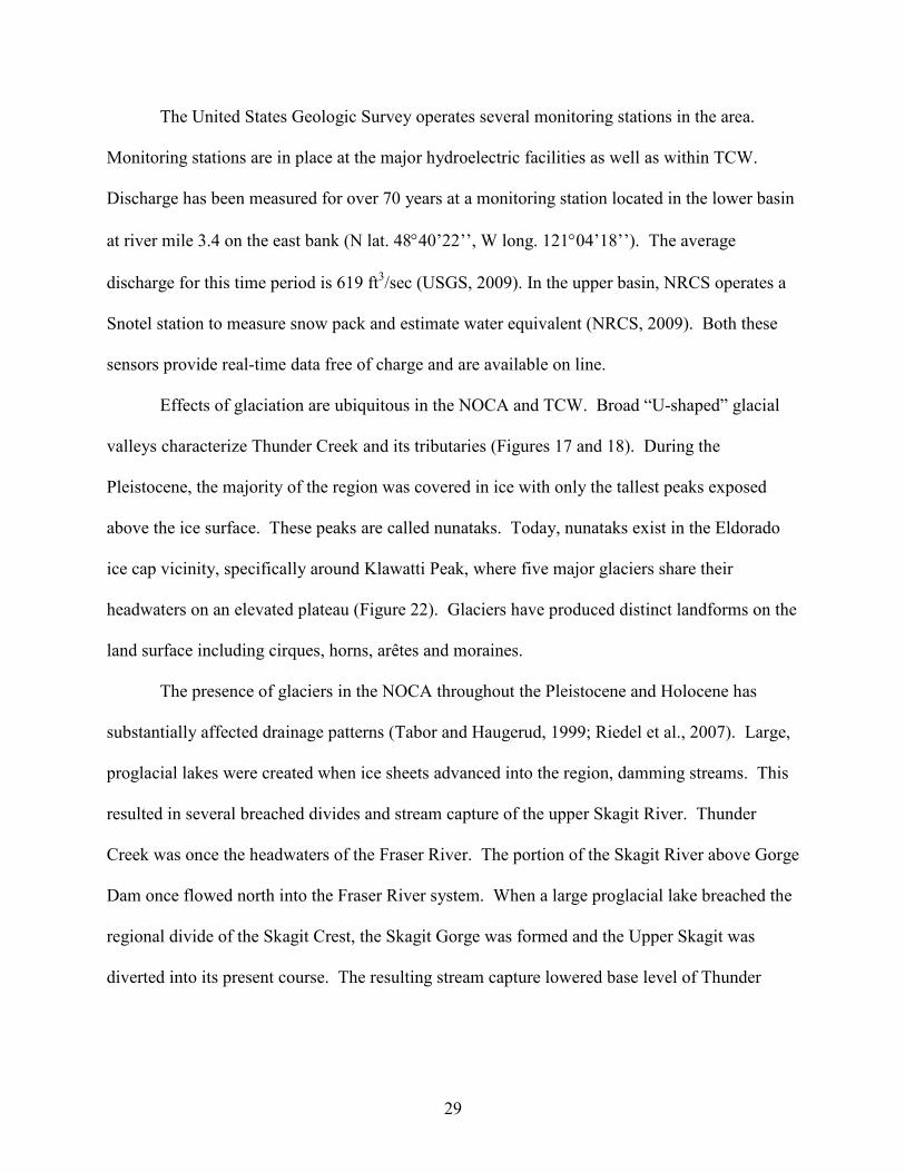
Stream profiles are useful for assessing the glacial history of a valley. Stream profiles
(Figures 19 and 20) differ from valley profiles (Figures 17 and 18) in that stream profiles follow
27
drainage patterns while valley profiles display interpolated elevation values collected along a
transect. Valleys with substantial glacial influences produce stepped valleys; examples include
the West fork of Thunder Creek (Figure 19) and the South fork of Fisher Creek (No Name
Creek, Figure 16). Beginning at Moraine Lake, the West Fork descends through several glacial
steps before terminating into the main stem of Thunder Creek. This is a stark contrast to a
typical, non-glaciated valley that has a smoother stream profile (Figure 20). Rhode creek is fault
controlled and lacks the stepped stream profile indicative of a glacially carved valley.
Figure 19. Stream profile graph of the West fork of Thunder Creek (elevation and distance in
m).
Figure 20. Stream profile graph of Rhode Creek (elevation and distance in m).

28
Stream orders are also useful in understanding the regional hydrology (Figure 21).
Higher order streams follow regional patterns determined by geologic substrate. This is evident
in streams that have northwest to southeast trending directions, such as Thunder Creek. Other
streams in the NOCA that exhibit this northwest to southeast trend are Cascade River, Goodell
Creek and Granite Creek. However, most first order streams have parallel patterns draining
steep valley walls.
Figure 21. Stream order of Thunder creek and its tributaries (1
st order = red, 2
nd order= orange,
3d order = green, 4th order = light blue, 5
th order = dark blue).
29
The United States Geologic Survey operates several monitoring stations in the area.
Monitoring stations are in place at the major hydroelectric facilities as well as within TCW.
Discharge has been measured for over 70 years at a monitoring station located in the lower basin
at river mile 3.4 on the east bank (N lat. 48°40’22’’, W long. 121°04’18’’). The average
discharge for this time period is 619 ft3/sec (USGS, 2009). In the upper basin, NRCS operates a
Snotel station to measure snow pack and estimate water equivalent (NRCS, 2009). Both these
sensors provide real-time data free of charge and are available on line.
Effects of glaciation are ubiquitous in the NOCA and TCW. Broad “U-shaped” glacial
valleys characterize Thunder Creek and its tributaries (Figures 17 and 18). During the
Pleistocene, the majority of the region was covered in ice with only the tallest peaks exposed
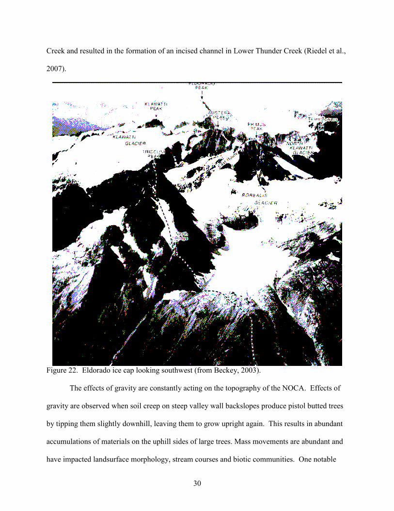
above the ice surface. These peaks are called nunataks. Today, nunataks exist in the Eldorado
ice cap vicinity, specifically around Klawatti Peak, where five major glaciers share their
headwaters on an elevated plateau (Figure 22). Glaciers have produced distinct landforms on the
land surface including cirques, horns, arêtes and moraines.
The presence of glaciers in the NOCA throughout the Pleistocene and Holocene has
substantially affected drainage patterns (Tabor and Haugerud, 1999; Riedel et al., 2007). Large,
proglacial lakes were created when ice sheets advanced into the region, damming streams. This
resulted in several breached divides and stream capture of the upper Skagit River. Thunder
Creek was once the headwaters of the Fraser River. The portion of the Skagit River above Gorge
Dam once flowed north into the Fraser River system. When a large proglacial lake breached the
regional divide of the Skagit Crest, the Skagit Gorge was formed and the Upper Skagit was
diverted into its present course. The resulting stream capture lowered base level of Thunder
30
Creek and resulted in the formation of an incised channel in Lower Thunder Creek (Riedel et al.,
2007).
Figure 22. Eldorado ice cap looking southwest (from Beckey, 2003).
The effects of gravity are constantly acting on the topography of the NOCA. Effects of
gravity are observed when soil creep on steep valley wall backslopes produce pistol butted trees
by tipping them slightly downhill, leaving them to grow upright again. This results in abundant
accumulations of materials on the uphill sides of large trees. Mass movements are abundant and
have impacted landsurface morphology, stream courses and biotic communities. One notable
31
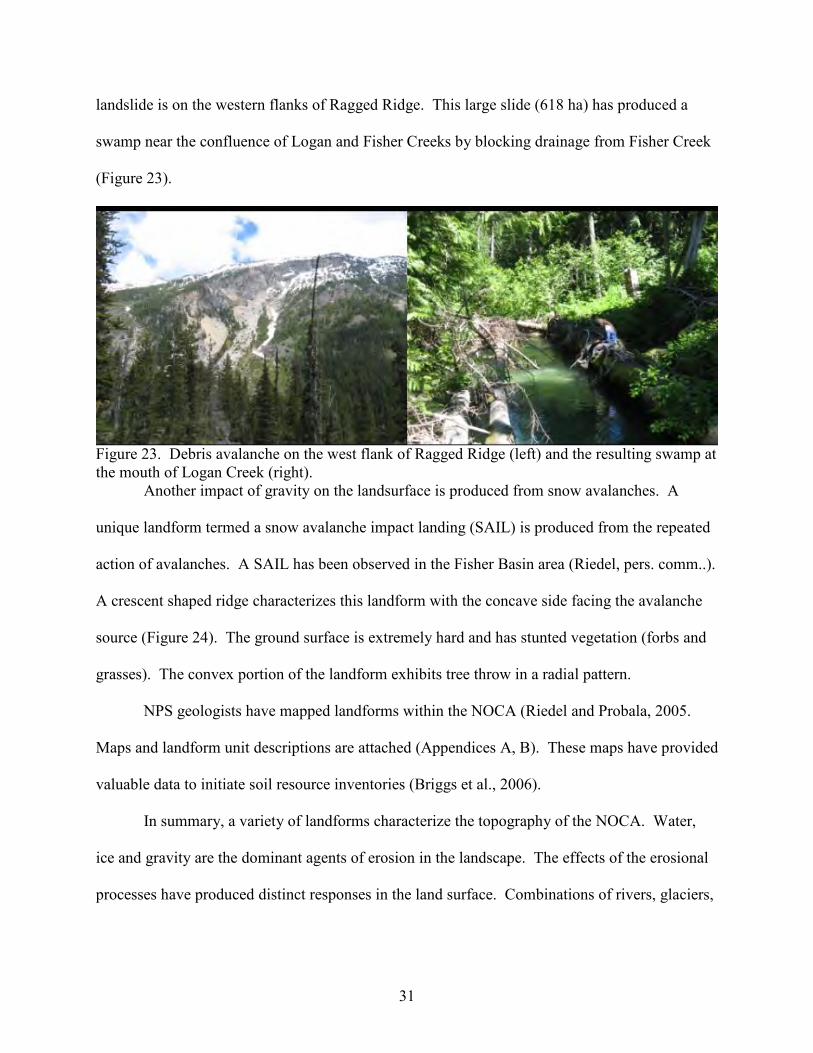
landslide is on the western flanks of Ragged Ridge. This large slide (618 ha) has produced a
swamp near the confluence of Logan and Fisher Creeks by blocking drainage from Fisher Creek
(Figure 23).
Figure 23. Debris avalanche on the west flank of Ragged Ridge (left) and the resulting swamp at
the mouth of Logan Creek (right).
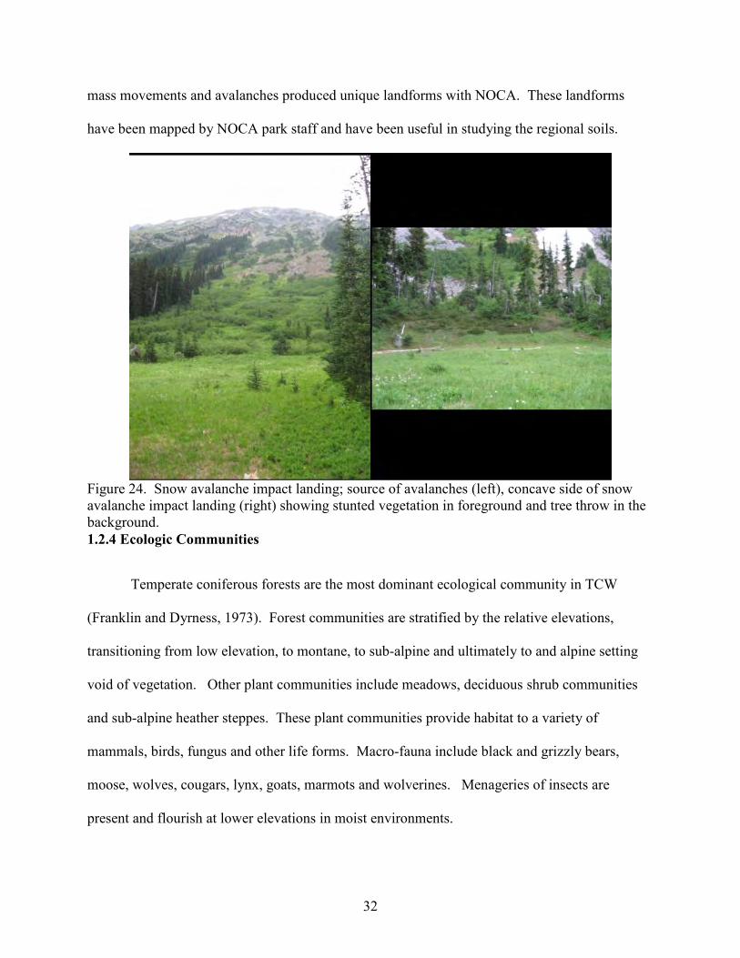
Another impact of gravity on the landsurface is produced from snow avalanches. A
unique landform termed a snow avalanche impact landing (SAIL) is produced from the repeated
action of avalanches. A SAIL has been observed in the Fisher Basin area (Riedel, pers. comm..).
A crescent shaped ridge characterizes this landform with the concave side facing the avalanche
source (Figure 24). The ground surface is extremely hard and has stunted vegetation (forbs and
grasses). The convex portion of the landform exhibits tree throw in a radial pattern.
NPS geologists have mapped landforms within the NOCA (Riedel and Probala, 2005.
Maps and landform unit descriptions are attached (Appendices A, B). These maps have provided
valuable data to initiate soil resource inventories (Briggs et al., 2006).
In summary, a variety of landforms characterize the topography of the NOCA. Water,
ice and gravity are the dominant agents of erosion in the landscape. The effects of the erosional
processes have produced distinct responses in the land surface. Combinations of rivers, glaciers,
32
mass movements and avalanches produced unique landforms with NOCA. These landforms
have been mapped by NOCA park staff and have been useful in studying the regional soils.
Figure 24. Snow avalanche impact landing; source of avalanches (left), concave side of snow
avalanche impact landing (right) showing stunted vegetation in foreground and tree throw in the
background.
1.2.4 Ecologic Communities
Temperate coniferous forests are the most dominant ecological community in TCW
(Franklin and Dyrness, 1973). Forest communities are stratified by the relative elevations,
transitioning from low elevation, to montane, to sub-alpine and ultimately to and alpine setting
void of vegetation. Other plant communities include meadows, deciduous shrub communities
and sub-alpine heather steppes. These plant communities provide habitat to a variety of
mammals, birds, fungus and other life forms. Macro-fauna include black and grizzly bears,
moose, wolves, cougars, lynx, goats, marmots and wolverines. Menageries of insects are
present and flourish at lower elevations in moist environments.
33
The vegetation of the region is characterized by the Western Hemlock (Tsuga heteropylla
or Tshe) forest alliance. This is the dominant forest type over the lower, western flank of the
Cascade Range. Another major species throughout the region is the Douglas-fir (Pseudotsuga
menziesii or Psme). These species exist roughly between 600 and 1200 m (2000 to 4000 ft) in
elevation. Psme exists on drier and/or more disturbed landscapes, while Tshe is the most shade-
tolerant species and can successfully out-compete Psme. Old-growth stands support Tshe or
Psme with an actively reproducing Tsme understory. Another associated species in the low
elevation forest is Western Red Cedar (Thuja Plicata or Thpl). Cedars can be found in and along
stream channels in wetter landscape positions, or along avalanche chute and rocky areas.
At higher elevations, different species emerge as principle forest types. These species
include the Pacific Silver Fir (Abies amabilis or Abam), the Mountain Hemlock (Tsuga
mertensiana or Tsme), and the Sub-alpine Fir (Abies lasiocarpa or Abla). Elevation zones range
from 750 to 1375 m (2500 to 4500 ft) for Abam, 900 to 1525 m (3000 to 5000 ft) for Tsme and
1300 to 1825 m (4300 to 6000 ft) for Abla. Montane forest communititesa also differ in
moisture and temperature of their respective microclimates. Other associated species include
Western Larch (Larix occidentalis), Engelmann Spruce (Picea engelmannii), and Alaskan
Yellow Cedar (Chamaecyparis nootkatensis).
The PNW, and more specifically the NOCA, are home to some of the worlds only
temperate rainforests. These forests are extremely productive and are characterized as “old
growth”. The mouth of Thunder Creek contains old growth stands of Psme, Tshe and Thpl.
These trees are exceptionally large and live up to 1,000 years (Pojar and MacKinnon, 1994).
In addition to coniferous forests, there are many broadleaf species as well. These include
Red Alder, Black Cottonwood, Big-leaf Maple, Mountain Ash, Sitka Alder, and Vine Maple.
34
There exists a patchwork of meadows, mosses, heather, and shrubs up to tree line. A list of
identified plant species is presented (Appendix C). Common growth forms include coniferous
trees, deciduous trees, shrubs, wildflowers, ferns, graminoids and mosses.
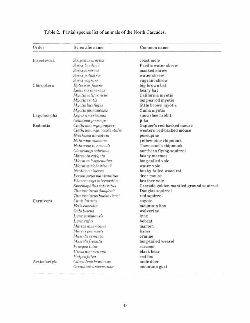
Plant communities provide habitat and nutrition for a variety of animals. A partial list of
animal species has been compiled (Table 2). A variety of fungi and molds are represented in the
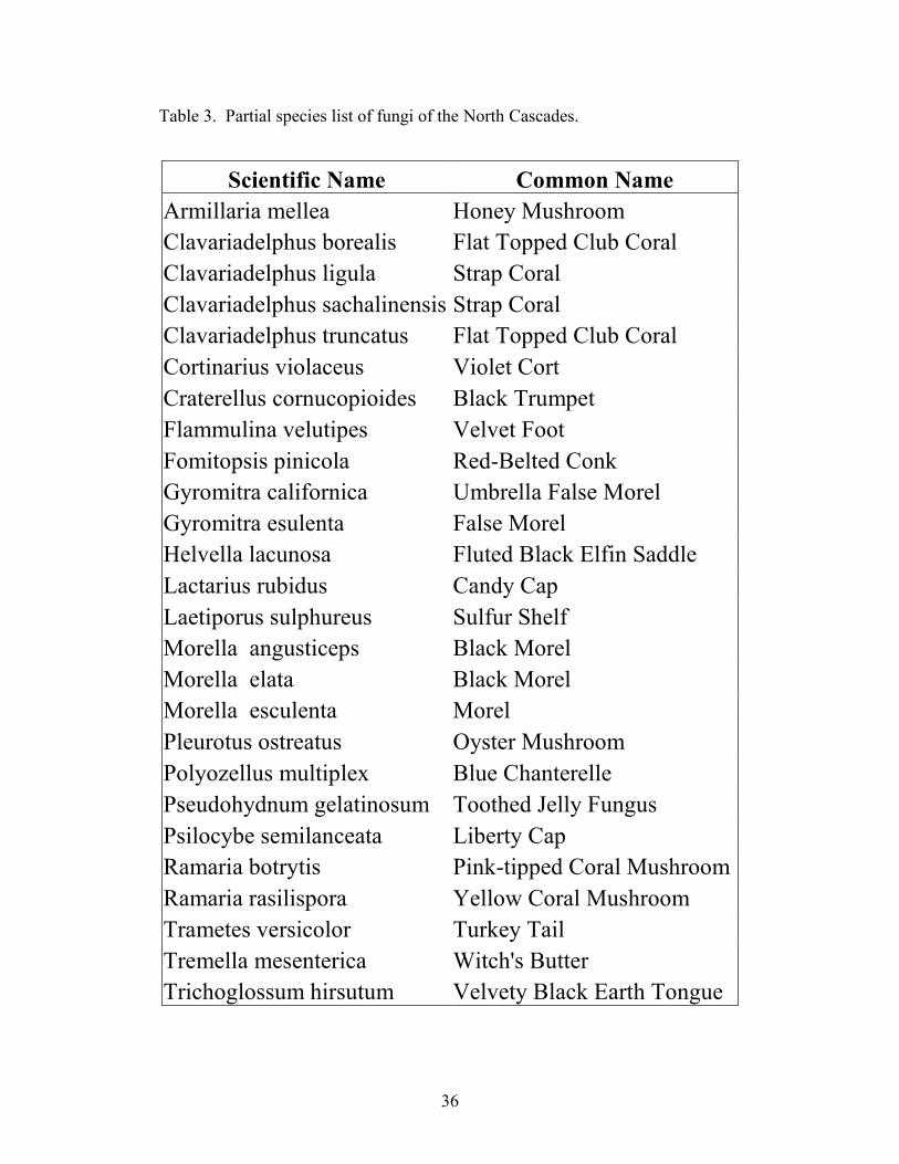
NOCA. Abundant moisture and woody debris provide a habitat suitable to the growth of fungi.
A total of 26 species of fungi representing 19 different genera have been identified (Table 3.)
1.2.5 Effects of Time and Human History
Time may be the most complex of Jenny’s factors to understand. Many influences can
determine the age of a landscape and the ages of the plants growing on a surface. The geologic
substrate provides the initial measure of time. The rocks from exotic terranes have been in place
since the end of the tertiary period and have experienced intense deformation and erosion.
Glacial movements have influenced the time of soil formation during the Pleistocene epoch.
More recent deposits include mass movements, alluvial sediments and the moraines of glaciers.
These agents continue to alter the landscape today, and control times of soil development.
In addition to the geologic processes that control the time of soil formation, forest fires
greatly influence the landscape. Following a burn, a landscape may be more prone to erosion
and mass wasting. Subsequently, pioneering plant species will colonize the area and begin the
process of biological succession. More recently, human influence has been seen in the region.
Logging has greatly influenced the patterns of succession. An important distinction is that there
is no logging within the NOCA, however, timber harvesting is currently being practiced outside
the park borders.
35
Table 2. Partial species list of animals of the North Cascades.
36
Table 3. Partial species list of fungi of the North Cascades.
Scientific Name Common Name
Armillaria mellea Honey Mushroom
Clavariadelphus borealis Flat Topped Club Coral
Clavariadelphus ligula Strap Coral
Clavariadelphus sachalinensis Strap Coral
Clavariadelphus truncatus Flat Topped Club Coral
Cortinarius violaceus Violet Cort
Craterellus cornucopioides Black Trumpet
Flammulina velutipes Velvet Foot
Fomitopsis pinicola Red-Belted Conk
Gyromitra californica Umbrella False Morel
Gyromitra esulenta False Morel
Helvella lacunosa Fluted Black Elfin Saddle
Lactarius rubidus Candy Cap
Laetiporus sulphureus Sulfur Shelf
Morella angusticeps Black Morel
Morella elata Black Morel
Morella esculenta Morel
Pleurotus ostreatus Oyster Mushroom
Polyozellus multiplex Blue Chanterelle
Pseudohydnum gelatinosum Toothed Jelly Fungus
Psilocybe semilanceata Liberty Cap
Ramaria botrytis Pink-tipped Coral Mushroom
Ramaria rasilispora Yellow Coral Mushroom
Trametes versicolor Turkey Tail
Tremella mesenterica Witch's Butter
Trichoglossum hirsutum Velvety Black Earth Tongue
37
Regional soils follow a pattern of succession similar to those observed by plant
communities. More active landscapes produce younger soil (Entisols and Inceptisols) while
stable forested landscapes support Spodosols. Although these ages are difficult to date
quantitatively, they provide a relative measure of the age of a soil or landsurface.
Absolute ages can be determined from specific events in the regional history. Mazama
tephra, Glacier Peak tephras and Mount Saint Helens tephra have been observed in the region.
The eruptions of Cascades Volcanoes provide a tool for dating ash layers in soils (Figure 25).
Tephrachronology has been used for dating in numerous studies including archaeology and
paleoclimatic reconstructions.
Human history is essential for understanding the role of the NOCA in our society.
Humans have occupied the region as early as 8,500 ybp (Mierendorf, 1998). Most prehistoric
inhabitants were ancestors of the Coast Salish tribes. Mountain passes such as Cascade Pass
provided important corridors for travel and trade between groups on opposite sides of the
Cascade Crest. Currently there are over 260 archeological sites within the park.
One of the earliest European explorers in the Region was Alexander Ross, who possibly
crossed the NOCA in 1848 (Beckey, 2003). Ross was a member of John Jacob Astor’s Pacific
Fur Company. The fur trade had an important role in the exploration of the Pacific Northwest.
The region became part of the United States in 1846 with the establishment of the Oregon
Territory (Beckey, 2003). Another expedition to explore the region was organized by Otto
Klement in 1877 and crossed the NOCA via Cascade Pass investigating gold in the Methow
Valley.

38
Figure 25. Dates of major eruptions of Cascade Volcanoes.
Mining prospectors played an important role in opening trails into the NOCA and
establishing mining claims. In the late 1880s, several explorers established mining claims in the
Cascade River drainage. These include the Horseshoe Basin, Doubtful Basin, and the Boston
and Chicago Mines. However, by 1919 most of the Thunder Creek mining companies had failed
due to the high cost of transporting ore to the smelter. In the 1890s several railroad surveyors
also ventured into the NOCA, but were turned away unsuccessful.
Also in the late 1890s, federal and state agencies began to preserve land in the Pacific
Forest Reserve and the Washington Forest Reserve, respectively. These were later transferred to

39
the USFS upon its creation in 1905. Seattle City Light received permission for the hydroelectric
projects in 1917 from the USDA. A road was constructed to Newhalem by 1921. The period
from 1935 to 1950 was characterized by further exploration into the high country and building of
a trail network by such rangers as Tommy Tompson and Lage Wernstedt (Beckey, 2003).
Hermann Ulrichs was a mountaineer who explored Thunder Creek in 1932 and pioneered many
of the first ascents of prominent peaks in the NOCA. The North Cascades Highway, the 89
miles of Washington State Route 20 between Marblemount and Twisp, was built from 1959 to
1972.
The NOCA-NP complex was established in 1968 by the 90th Congress and signed into
law by President Johnson. The NOCA-NP Complex is composed of the NOCA-NP north and
south units (combined area of 204,000 ha) and the Ross Lake and Lake Chelan National
Recreation Areas (69,000 ha).
1.2.6 Other Models of Soil Formation
The majority of this section comes from McBratney et al. (2003). The SCORPAN model
is similar to the soil-factor model proposed by Jenny (1941), but has some additions. In this
model of soil formation, soil attributes and/or soil classes (Sa, Sc) are a function of s,c,o,r,p,a,n
where s stands for soil (including existing soil information), c stands for climate, o represents
organisms, r stands for relief, p represents parent materials and lithology, a represents age and n
represents the spatial dimension. This model is inherently similar to Jenny’s model except for
the inclusion of spatial dimensions and existing soil information. These differences may seem
trivial at first, but are relevant in many digital soil mapping applications. Most digital soil maps
are produced with geographic information systems (GIS). These technologies allow spatial
40
phenomenon to be clearly displayed, manipulated and quantitatively analyzed (i.e., analyses of
spatial autocorrelation of residuals). Also, the SCORPAN model includes a soil factor. This
factor is becoming increasingly important as soil resources inventories are being conducted
around the globe (Legacherie et al., 1995). This legacy data is valuable in contemporary digital
soil mapping applications. These slight modifications to Jenny’s model have modernized the
concepts of soil genesis to better work with today’s digital technologies.
Many conceptual models exist for describing natural phenomenon. Some are site specific
while others are broader in their focus. I have used various models to aid in the understanding of
soil-water-gravity interactions in TCW. I am looking at soils and landforms and use these
conceptual models to facilitate my understanding of the underlying processes. These models
provide a framework for understanding the complexities of natural systems and how they vary
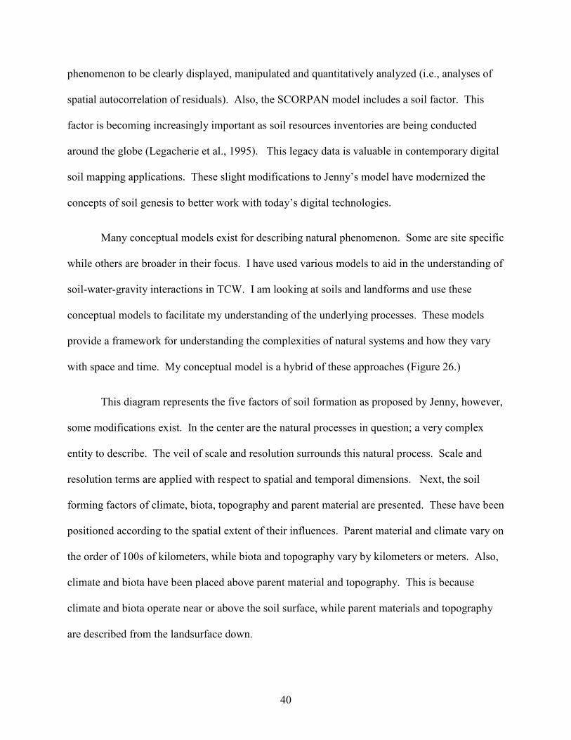
with space and time. My conceptual model is a hybrid of these approaches (Figure 26.)
This diagram represents the five factors of soil formation as proposed by Jenny, however,
some modifications exist. In the center are the natural processes in question; a very complex
entity to describe. The veil of scale and resolution surrounds this natural process. Scale and
resolution terms are applied with respect to spatial and temporal dimensions. Next, the soil
forming factors of climate, biota, topography and parent material are presented. These have been
positioned according to the spatial extent of their influences. Parent material and climate vary on
the order of 100s of kilometers, while biota and topography vary by kilometers or meters. Also,
climate and biota have been placed above parent material and topography. This is because
climate and biota operate near or above the soil surface, while parent materials and topography
are described from the landsurface down.
41
Figure 26. Conceptual model of soil formation adapted for the North Cascades.
This diagram is very useful for understanding pedogenic properties in TCW. However,
when posed with questions concerning other natural phenomenon (ecology, solar radiation,
atmospheric pressure systems, etc.) this diagram helps to visualize the interdependence of these
factors and the complexity inherent in nature.
42
1.3 Soils of the North Cascades
Soils from the NOCA exhibit unique combinations of parent materials and pedogenic
processes. Few places in the world have podsolization occurring in volcanic tephra rich parent
materials. These include the PNW, Alaska, Eastern Russia, Northern Japan, and New Zealand
(Briggs et al., 2006). Soils are here described first by the bedrock geology, weathering of parent
materials, and formation of primary and secondary minerals within soil environments. Next,
important pedogenic processes are discussed. Soils are described with respect to the ecological
characteristics and niches. Finally, regional soils are discussed with respect to classification and
mapping.
Bedrock geology is rarely the sole parent material for soils in TCW. Few residual soils
exist, however, they are generally found in alpine environments, are very shallow, and are
dominated by rock fragments larger than 2mm in diameter. More commonly, soil parent
material is influenced by organic matter, volcanic ash and glacial till. Forested locations produce
abundant leaf litter and provide organic soil horizons above most mineral soils. Volcanic ash
mantles are present throughout the region and influence soils due to the high specific surface
area of short-range order minerals (SROM) (Dahlgren and Ugolini, 1991; McDaniel et al., 1994;
McDaniel et al., 2005). Glacial till is frequently a secondary parent material, found below the
ash mantle.
Moderate temperatures and abundant moisture accelerate weathering of parent materials.
Physical erosion is commonly observed in mass movements. Chemical erosion is evident in the
E-Bs horizon sequence found in many Spodosols. Rapid chemical alterations occur as soil parent
materials are altered into primary and secondary soil minerals.
43
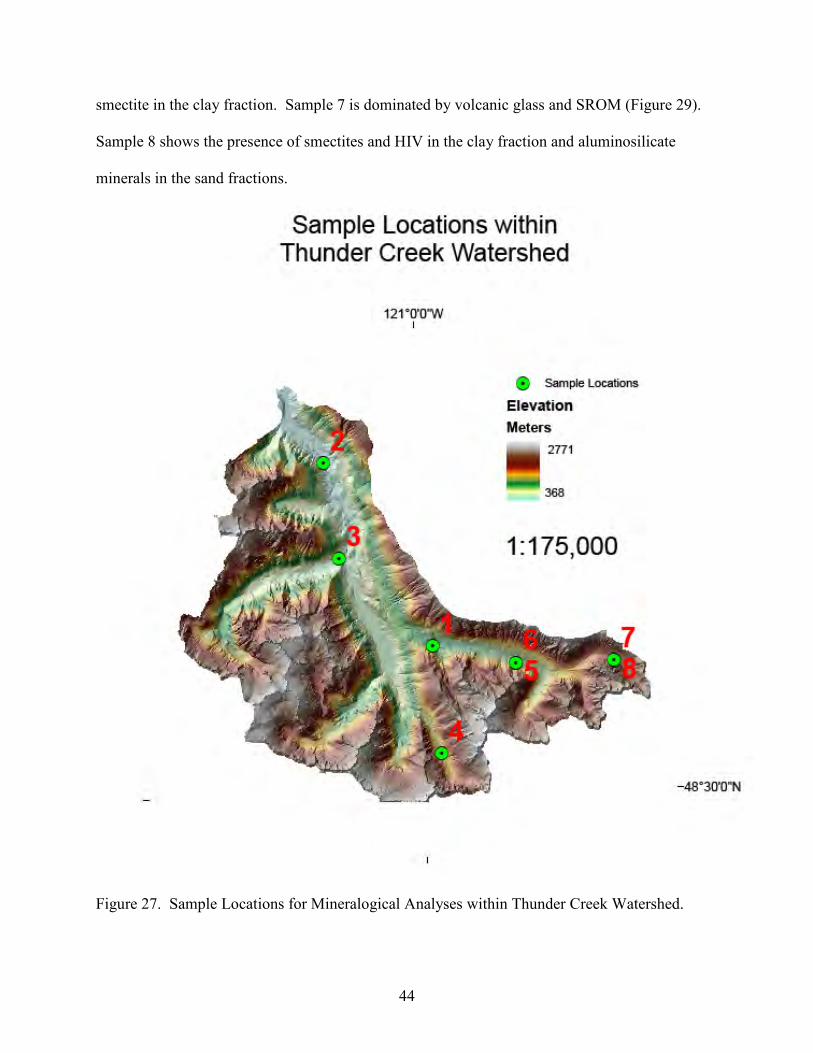
I have characterized soil mineralogy through my work at the University of Idaho. Of the
over 400 soil samples collected from TCW, eight were selected for mineralogical analysis.
Samples were chosen based on reflectance in the visible and near-infrared (Vis-NIR) regions of
the spectrum using VisNIR-diffuse reflectance spectroscopy (DRS, Sankey et al., 2008).
Reflectance profiles were clustered using partitioning around mediods on the Mahalanobis
distances of the first derivative of reflectance (Kaufman and Rousseeuw, 1990). All organic soil
horizons (Oi, Oe) were excluded from the statistical selection methods. Eight clusters were
created and a single sample was randomly selected from each (Figure 27).
The information gained from mineralogical investigations provides insights to the
pedogenic environments and processes within TCW. From the various analyses conducted at the
University of Idaho, data have been collected with regard to minerals present in selected soils.
Mineralogical analyses include particle size analysis, selective dissolution, X-ray diffraction,
total elemental analysis, petrographic microscopy, and scanning electron microscopy with energy
dispersive X-ray spectroscopy.
Sample 1 exhibits X-ray diffraction (XRD) patterns indicative of chlorite, mica, kaolinite
and hydroxy-interlayered vermiculite in the clay size fraction. Sample 2 XRD patterns show
kaolinite and SROM in the clay size fraction. XRD results from Sample 3 suggest chlorite,
mica, kaolinite, hydroxy-interlayered vermiculite and hydroxy-interlayered smectite are present.
Sample 4 exhibits XRD patterns characteristic of chlorite, mica and hydroxy-interlayered
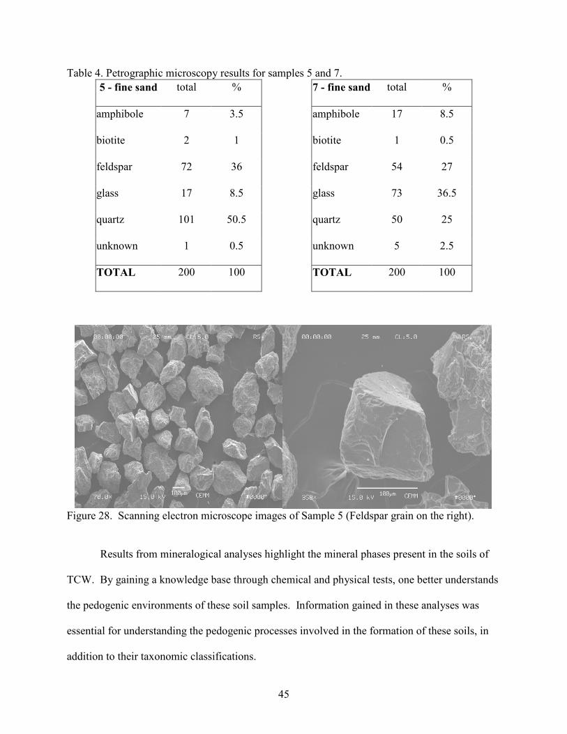
vermiculite. Sample 5 shows the presence of kaolinite, vermiculite, chlorite, HIV and possibly
smectite minerals in the clay fraction and mostly quartz and feldspar, with some volcanic glass,
in the fine sand fraction (Table 4, Figure 28). Sample 6 is dominated mostly by primary
minerals in the sand fractions and contains kaolinite, vermiculite, chlorite, HIV, mica and
44
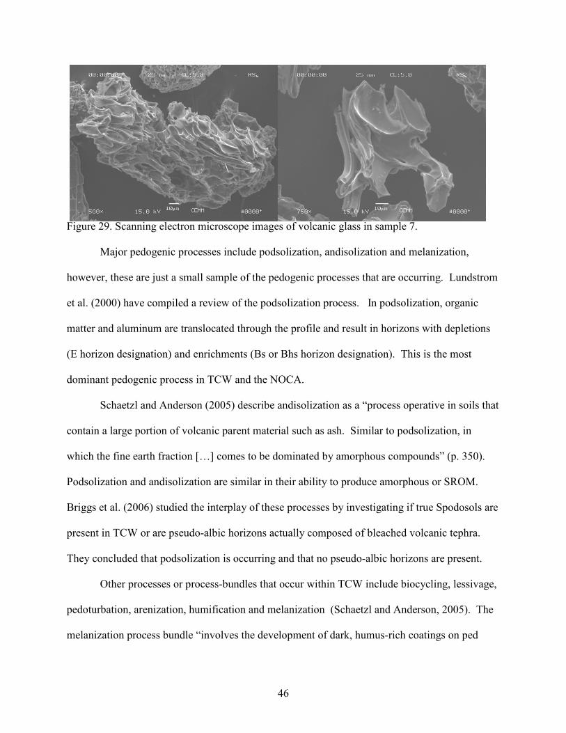
smectite in the clay fraction. Sample 7 is dominated by volcanic glass and SROM (Figure 29).
Sample 8 shows the presence of smectites and HIV in the clay fraction and aluminosilicate
minerals in the sand fractions.
Figure 27. Sample Locations for Mineralogical Analyses within Thunder Creek Watershed.
45
Table 4. Petrographic microscopy results for samples 5 and 7.
5 - fine sand total % 7 - fine sand total %
amphibole 7 3.5 amphibole 17 8.5
biotite 2 1 biotite 1 0.5
feldspar 72 36 feldspar 54 27
glass 17 8.5 glass 73 36.5
quartz 101 50.5 quartz 50 25
unknown 1 0.5 unknown 5 2.5
TOTAL 200 100 TOTAL 200 100
Figure 28. Scanning electron microscope images of Sample 5 (Feldspar grain on the right).
Results from mineralogical analyses highlight the mineral phases present in the soils of
TCW. By gaining a knowledge base through chemical and physical tests, one better understands
the pedogenic environments of these soil samples. Information gained in these analyses was
essential for understanding the pedogenic processes involved in the formation of these soils, in
addition to their taxonomic classifications.
46
Figure 29. Scanning electron microscope images of volcanic glass in sample 7.
Major pedogenic processes include podsolization, andisolization and melanization,
however, these are just a small sample of the pedogenic processes that are occurring. Lundstrom
et al. (2000) have compiled a review of the podsolization process. In podsolization, organic
matter and aluminum are translocated through the profile and result in horizons with depletions
(E horizon designation) and enrichments (Bs or Bhs horizon designation). This is the most
dominant pedogenic process in TCW and the NOCA.
Schaetzl and Anderson (2005) describe andisolization as a “process operative in soils that
contain a large portion of volcanic parent material such as ash. Similar to podsolization, in
which the fine earth fraction […] comes to be dominated by amorphous compounds” (p. 350).
Podsolization and andisolization are similar in their ability to produce amorphous or SROM.
Briggs et al. (2006) studied the interplay of these processes by investigating if true Spodosols are
present in TCW or are pseudo-albic horizons actually composed of bleached volcanic tephra.
They concluded that podsolization is occurring and that no pseudo-albic horizons are present.
Other processes or process-bundles that occur within TCW include biocycling, lessivage,
pedoturbation, arenization, humification and melanization (Schaetzl and Anderson, 2005). The
melanization process bundle “involves the development of dark, humus-rich coatings on ped

47
faces and mineral grains, rendering the horizon a dark brown or black color” (p. 356, Schaetlz
and Anderson, 2005).
When discussing soil genesis and profile development, one must place the soils of TCW
into an ecological context. Meirik (2008) has shown statistical correlations between soil
properties and vegetation. To place the soils in an ecological setting, I will use the concept of
Potential Natural Vegetation (PNV) as an analogy. To understand PNV, one must understand
successional patterns and an ecosystem’s response and recovery to large scale changes (i.e.,
landslides, fires, logging, etc.). I propose that a landsurface in TCW will mature into a low
elevation forest composed of western hemlock, Douglas-fir and western red cedar if it remains
undisturbed. This forest association is the PNV for sites in TCW below 1,250 m in elevation.
Following a stand clearing disturbance, vegetation will respond by colonization of pioneering
plant species, namely alders, maples, and grasses. Alders have the ability to biologically fix
nitrogen due to symbiotic relationships with soil micro-organisms. Alders are well suited to
growth in nutrient-poor soil environments. As this plant community matures, red cedar or
perhaps lodgepole pine may be the first coniferous trees to establish themselves. These species
are then followed by Douglas-fir and hemlocks. Given sufficient time to reach a climax stage,
hemlocks will mature and compete with Douglas-firs as the most dominant species.
This chain of ecological succession is analogous to the development of soils on disturbed
landsurfaces within TCW. Following a landslide or avalanche, all soil material is removed. This
fresh landsurface is composed of rock fragments, which develop moss coatings. The moss layers
are frequently enriched by litter from nearby plants and form young, shallow soils (Lithic
Udifolists). When pioneering plant species, such as alders, colonize the fresh landsurface,
melanization is evident. These profiles eventually develop into Entisols and Inceptisols. Given

48
sufficient time and landsurface stability, podsolization may shift the pedogenic controls and
produce a Spodosol. This mature Spodosol is analogous to the mature stand of hemlocks and
Douglas-fir trees that are described as PNV. The well-devolved Spodosol could be termed the
“potential natural soil” for this environment.
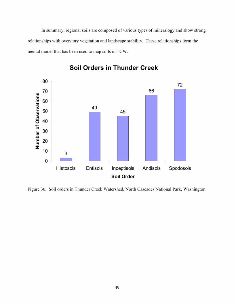
North Cascade soils are composed of a complex mixture of several soil orders, including
Spodosols, Andisols, Inceptisols, Entisols and Histosols (Figure 30). As previously discussed
with regards to ecological succession, landscape stability plays a large role in the development of
these soils. Major pedogenic controls have been outlined by Briggs (2004) and Briggs et al.
(2006), and include erosional and depositional history, over-story vegetation, and temperature.
They found stable landforms (bedrock benches and Pleistocene moraines) had a higher
occurrence of Spodosols. Andisols and Spodosols dominated landsurfaces characterized by
active colluvial additions (debris aprons and valley walls). Inceptisols dominated landforms
influenced by water erosion (debris cones, alluvial fans and terraces). Entisols and Histosols are
found on unstable surfaces and are related with zones of mass wasting.
Briggs (2004; 2006) used these pedogenic processes to map soils in the watershed
(Figure 31). She employed an expert-knowledge, rule-based system to map soils corresponding
to a 4th order soil survey using traditional landform maps, DEM derived terrain attributes and
remotely sensed land cover classifications. Soils were mapped at the sub-group level and map
units contain Spodosols, Andisols, Inceptisols and Entisols in addition to water, rock outcrops,
and ice. Landscape stability, land cover, and climate were identified as the dominant controls
on pedogenesis.
49
In summary, regional soils are composed of various types of mineralogy and show strong
relationships with overstory vegetation and landscape stability. These relationships form the
mental model that has been used to map soils in TCW.
Figure 30. Soil orders in Thunder Creek Watershed, North Cascades National Park, Washington.
Soil Orders in Thunder Creek
3
4945
66
72
0
10
20
30
40
50
60
70
80
Histosols Entisols Inceptisols Andisols Spodosols
Soil Order
Number of Observations

50
Figure 3
1. D
igital so
il map of T
hunder C
reek W
atershed created
by Brig
gs (2
004).
51
1.4 Literature Review
The application of digital technologies to traditional methods of soil survey has created
digital soil mapping (DSM). McBratney et al. (2003) and Scull et al. (2003) have compiled
reviews of DSM. DSM relies on the hypothesis that quantitative environmental variables are
correlated with the spatial distribution of soil classes and properties. Combinations of landform
and land cover are common tools for soil mapping (Dobos et al., 2000; McKenzie and Ryan,
1999; Hengl and Rossiter, 2003). Correlations between environmental factors and soil profile
characteristics allow a surveyor to extrapolate knowledge from a profile observation to a
landscape. The ability of a soil surveyor to correlate soil distribution with readily observed
environmental factors (landform and land cover) allows for the mapping of soil entities over
large areas with minimal soil profile observations.
It is important to use environmental covariates that are easily and inexpensively
observable at many spatially referenced locations. For example McBratney et al. (2003) use the
following equation to generalize DSM:
S[x,y]=f(Q[x,y]) + e[x,y]
where, S is a soil property of interest, Q are environmental covariates represented by raster layers
in a GIS software, f is a empirical quantitative function linking S and Q, and e are the errors.
Inherent in the above equation are spatial dimensions associated with S, Q and e. Observations
of Q must be much larger than the number of observations of S for efficient use of DSM
(McBratney et al., 2003).
Many of the processes involved with the formation of soils are similar to the processes
involved in landform formation, namely soil-water-gravity interactions. The connections
between geomorphology, hydrology and pedology have been recognized for almost a century.
52
Early research into soils and geomorphology recognized the important link between soils and
landforms (Milne, 1935). Ruhe (1961) segmented landforms into four elements, uplands,
backslopes, footslopes and toeslopes. In Iowa, Ruhe’s landform elements correlated with soil
properties, including clay content and weathering indices. Ruhe’s model was later expanded to a
nine-unit landsurface model, with landsurface units showing correlation to soil properties in
Australia, New Zealand, the United Kingdom, and Uganda (Conacher and Dalrymple, 1977).
Conacher and Dalrymple (1977) have coined the term “pedogeomorphology” to make this
linkage even more explicit. Their nine-unit landsurface model has been adapted for use in DLM
(Park et al., 2001).
For DSM, quantitative descriptions of soil-water-gravity interactions are achieved
through two distinctly different approaches. The first approach is a hydrology approach (Beven
and Kirby, 1979; Moore et al., 1993; Tarboton, 1991). This method uses the hypothesis that soil
development is related to the way water moves over and through a landscape (Moore et al.,
1993). By quantifying flow patterns through digital terrain analysis, one is able to make
inferences regarding soil attributes and class distribution.
A uniquely different approach is a geomorphology approach focusing on slope processes,
including detachment, transport and deposition of soil materials (Pennock et al., 1987;
MacMillan et al., 2000). This approach segments the surface into similar landforms with distinct
combinations and extents of various slope processes. This method of landscape segmentation
also makes inferences regarding the processes of formation for a given landform unit. The
geomorphic approach to DSM involves an understanding of landscape evolution when
describing the topography of a contemporary landsurface. Ultimately for application to DSM,
one hopes strong correlations exist between geomorphic units and soil attributes.
53
Both approaches rely on the distribution of water and how it moves through a landscape
to describe soil properties and classes. A key difference between these approaches is the
timeframe in which they operate. Most hydrologic methods rely on contemporary surface
morphology to describe water movements over short-term precipitation events. Conversely,
geomorphic approaches use surface morphology to describe processes that create landforms over
much larger periods of time. Using a hydrological approach for DSM, one seeks correlation
between surface/subsurface water movements and soil attributes. This research employs a
geomorphic approach to DSM.
The DEM is the fundamental backbone of terrain analysis because DEMs allow for the
simple manipulation of raster data sets. Topographic parameters like slope, curvature and aspect
are easily calculated from DEMs (Pennock et al., 1987). The first derivative of elevation is
equal to the slope of a surface, while the second derivative represents the curvature of a surface.
Terrain attributes like slope and curvature can be calculated from a DEM in seconds and can be
applied to large areas. While slope and curvature are relatively simple metrics derived from a
DEM, measures of solar insulation, contributing areas, and indices of wetness, stream power, and
sediment transport are also available. A distinction between primary and secondary terrain
attributes is used to signify metrics derived directly from elevation data and other metrics that
rely on primary terrain attributes (i.e., the use of slope in the calculation of wetness index). The
abundance of quantitative topographic information allows researchers to create their own indices
through mathematical manipulations of DEM-derived terrain attributes, for site specific uses.
Application of DEMs and terrain attributes to landform mapping has produced the
emerging field of digital landform mapping (DLM, Moore et al., 1993; Wood, 1996). This has
also been called geomorphometry (Hengl and Reuter, 2008), terrain analysis (Wilson and
54
Gallant, 2000), environmental correlation (McKenzie and Ryan, 1999) and many other monikers.
Reviews of geomorphometry have been compiled (Pike, 2000; Shary et al., 2002). A key
hypothesis of geomorphometry and DLM is that the shape of the land surface, observed by
remote sensing, is related with surficial geologic processes. These geologic processes include
detachment, transportation and deposition, the central tenants of erosion. These erosional
processes are enacted through various mechanisms yet produce distinct spatial entities, or
landforms. Individual repeating morphologic units are identified in the field and mapped as
landforms. Traditional methods of landform mapping involve the use of topographic maps and
aerial photographs. Initial lines are drawn onto topographic maps with the aid of stereo pairs of
photographs. These are then validated and modified through field observations (Riedel and
Probala, 2005). This has been completed for a majority of the North Cascades National Park.
Landform mapping has been used to identify endangered species habitat, geologic hazards, and
cultural resources within the North Cascades National Park (Riedel and Probala, 2005).
Examples of DLM and DSM exist through the globe (McBratney et al., 2003; Scull et al.,
2003). DLM in Saskatchewan was achieved by segmenting the landscape based on profile
curvature, plan curvature and slope gradient (Pennock et al., 1987). For this study, thickness of
A horizons and depth to calcium carbonate showed an overall increase in the sequence shoulder
< backslope < level < footslope elements. MacMillan et al. (2000) used fuzzy logic and heuristic
rules to digitally map landforms in Alberta. Resulting landform units were correlated with A
horizon depth and crop yields. Examples of DLM and DSM are abundant and exist across a
broad spectrum; from deductive (MacMillan et al., 2000; MacMillan et al., 2007; Cook et al.,
1996) to inductive (Dragut and Blaschke, 2006), from theoretical (Ehsani and Quiel, 2008) to
empirical (Saadat et al., 2008), and produce both fuzzy representations (Burrough et al., 1992;

55
Schmidt and Hewitt, 2004) and discrete choropleth maps (van Asselen and Seijmonsbergen,
2006).
Here I use empirical and inductive methods to produce discrete maps of landform
elements and soil properties. I have a large spatially registered database of over 400
observations of landforms. This volume of data is unprecedented for DLM in wilderness areas.
These data allow for robust statistical evaluations however, I must avoid over-fitting this model
to this specific watershed. To improve the transferability of this digital landform model I use
inductive methods to classify landforms based on DEM derived terrain attributes. Inductive
classifications provide rules for landform classification by seeking patterns within the data.
I hope the methods used here can be applied to map other humid, mountainous
landscapes, more specifically, the National Parks within Washington State: North Cascades,
Mount Rainer and Olympic Other federal lands in the PNW may also be within the scope of
these modeling tools. The North Cascades National Park Complex (composed of the national
park and Ross Lake and Lake Chelan National Recreation Areas) comprises the 40,000 ha core
of the North Cascade Ecosystem (National Park Service, 2003). This extends from the Puget
Sound to the Columbia River in the east and from the Fraser River to Snoqualmie Pass in the
south. Numerous wildernesses and national forests are present with only 2 major highways
crossing the region (US-2 and WA-20).
Through DSM and DLM, a quantitative description of the earth's surface is relatively
inexpensive and provides more information than was previously available. The vast amount of
data stored in DEMs and within DEM derived terrain attributes allows for the rapid
quantification of land surface features. Additional benefits of DSM and DLM compared with
traditional methods are that digital methods are more explicit (Hudson, 1992) and can easily

56
updated as newer or higher resolution data is available. The ubiquity of digital data allows for
archival into databases for evaluation of temporal changes in landsurface morphology and soil
attributes.
DSM has been applied to mapping soils in 90,000 ha of the Sawtooth and Pasayten
Wildernesses in Washington State (Rodgers, 2000) to map soils at the sub-group level of soil
taxonomy (Soil Survey Staff, 1999). Expert rules within a decision tree format were used to
classify soils based on landform and land cover digital data. Fourth order soil surveys (map
scale of 1:100,000) were produced and resulting soil taxa include Spodosols, Andisols, and
Inceptisols from xeric and udic moisture regimes. Rodgers found slope to be the most important
topographic attribute for prediction of soil classes. Other important predictors included land
cover, wetness index and profile curvature.
Ufnar (2004) mapped landtype associations (LTA) in the 13500 ha North Fork of the
Skykomish River on the Western Slope of the Central Cascades. This study was conducted
within the Henry M. Jackson Wilderness. LTAs are based on combinations of landforms,
geology, and potential natural vegetation (PNV), and represent units with similar ecological
processes, (Davis, 2004). LTAs fit within the National Hierarchical Framework of Ecological
Units and are generally mapped at scales from 1:250,000 to 1:62,500. The US Forest Services’
terrestrial ecosystems unit inventory (TEUI) geospatial toolkit was used to digitize landforms
based on digital layers representing landforms, geology and PNV. The PNV and geology layers
were obtained from the Mt Baker – Snoqualmie National Forest. Landforms were digitized on
screen by using high resolution digital ortho-quarter quads, LANDSAT images, DEM-derived
terrain attributes and 3D visualizations of digital data in GIS software. Ufnar then used LTAs to
map soil distribution at the sub-group level. Ufnar identified glacial history, volcanic tephra,

57
landform stability and land cover to be the dominant controls on pedogenesis. Fourth order soil
surveys were produced and resulting soil taxa include Spodosols, Andisols, and Inceptisols.
Briggs (2004, 2006) mapped soils in the 30,000 ha Thunder Creek Watershed (TCW)
using DSM. Expert knowledge and a rule based system were used to map soils corresponding to
a 4th order soil survey using traditional landform maps, DEM derived terrain attributes and
remotely sensed land cover classifications. Soils were mapped at the sub-group level and map
units contain Spodosols, Andisols, Inceptisols and Entisols in addition to water, rock outcrops,
and ice. Landscape stability, land cover, and climate were identified as the dominant controls
on pedogenesis.
Meirik (2008) returned to TCW to improve the accuracy of land cover maps to aid in
DSM. Land cover mapping was improved by using higher spatial and spectral resolution
satellite data. Meirik outlined a method of supervised classification of satellite images based on
field observations. This empirical method can be used to further improve land cover-mapping
accuracy for its use as a precursor to DSM. Meirik found thickness of O, A, E and Bs horizons
were statistically correlated with land cover classes.
In this work, I returned to TCW during the summer of 2007 and 2008 to describe and
classify landforms and soils. This work employs two inductive statistical classification
techniques to segment landform elements. I used binary decision trees (BDT) (Brieman, 1984),
and random forests (RF) (Brieman, 2001). These classification tools are inductive in nature,
allowing data to be analyzed without pre-conceived mapping rules. By seeking patterns within
the data, we can let the information speak for itself, without posing any a priori constraints. This
is in contrast to many digital mapping methods, which are either semi-automated (van Asselen

58
and Seijmonsbergen, 2006; Eshani and Quiel, 2008) or expert driven (Briggs et al., 2006;
MacMillan et al., 2000).
I assembled a digital database of over 400 GPS-referenced site descriptions of
geomorphology, soil profile descriptions, and plant communities from the work of Briggs
(2004), Meirik (2008) and myself. A large data set allows for robust statistical inferences in the
study area. Many digital models rely on little if any field observations (Eshani and Quiel, 2008;
van Asselen and Seijmonsbergen, 2006; Bolongaro-Crevenna et al., 2005; Irving et al., 1997).
1.5 Objectives
My study objectives were to: 1) use field observations to evaluate an existing expert
landform map, 2) calibrate and validate inductive classification methods for mapping landforms
in rugged mountainous terrain with field observations, 3) compare these inductive classifications
with an expert landform map and 4) seek statistical correlations between topographic information
(landform elements and DEM derived terrain attributes) and soil attributes (including taxonomic
classes and soil properties). By mapping soils in wilderness areas with DSM, I hope to propose a
method for completion of the soil survey in Washington State and ultimately the nation.
59
1.6 References:
Allen, John Elliot, Marjorie Burns and Sam C. Sargent. 1986. Cataclysms on the Columbia.
Timber Press, Portland Oregon.
Beckey, Fred. 1995. Cascade Alpine Guide, vol.(3), 2nd ed. The Mountaineers. Seattle, WA
Beckey, Fred. 2003. Cascade Alpine Guide, vol.(2), 3rd ed. The Mountaineers. Seattle, WA
Beven, K.J. and M.J. Kirby. 1979. A physically based, variable contributing area model of
basin hydrology. Hydrological Sciences 24:43-69.
Bolongaro-Crevenna, A., Torres-Rodriguez, V., Sorani, V., Frame, D., and Ortiz, M.A. 2005.
Geomorphometric analysis for characterizing landforms in Morelos State, Mexico.
Geomorphology 67:407-422.
Breiman, L., Friedman, J., Olshen, R., and Stone, C. 1984. Classification and regression trees.
Chapman and Hall/CRC, Boca Raton, FL.
Breiman, L. 2001. Random Forests. Machine Learning 45:5-32.
Briggs, C.A.D. 2004. GIS-Based mapping of soil distribution in Thunder Creek Watershed,
North Cascades National Park, Washington. Washington State University M.S. Thesis.
Briggs, C.A.D., Busacca, A.J. and McDaniel, P.A. 2006. Pedogenic processes and soil-
landscape relationships in North Cascades National Park, Washington. Geoderma
137:192-204.
Burrough, P.A. MacMillan, R.A. and van Deursen, W. 1992. Fuzzy land classification methods
for determining land suitability from soil profile observations and topography. Soil
Science 43:193-210.
Conacher, A.J. and Dalrymple, J.B. 1977. The nine-unit landsurface model: An approach to
pedogeomorphic research. Geoderma 18:1-154.
Cook, S.E., Corner, R.J., Grealish, G., Gessler, P.E. and Chartres, C.J., 1996. A rule-based
system to map soil properties. Soil Science Society of America Journal, 60(6): 1893-
1900.
Dahlgren, R.A. 1994. Quantification of Allophane and Imogolite. pp.430-451 In Quantitative
Methods in Soil Mineralogy, J.E. Ammonette and L.W. Zelazny (eds.) Soil Science
Society of America, Madison, WI.
Dahlgren, R.A. and F.C. Ugolini. 1991. Distribution and characterization of short-range order
minerals in Spodosols from the Washington Cascades. Geoderma 48:391-413.
60
Dobos, E., Micheli, E., Baumgardner, M.F., Biehl, L and Helt, T. 2000. Use of combined
digital elevation model and satellite radiometric data for regional soil mapping.
Geoderma 97:367-391.
Dragut, L. and Blaschke, T. 2006. Automated classification of landform elements using object-
based image analysis. Geomorphology 81:330-344.
Ehsani, A.H., and Quiel, F. 2008. Geomorphometric feature analysis using morphometric
parameterization and artificial neural networks. Geomorphology. 99:1-12.
Franklin, Jerry F., and C.T. Dyrness. 1973. Natural Vegetation of Oregon and Washington.
Gen. Tech. Rep. PNW-8. Portland, OR: U.S. Dept. of Agriculture, Forest Service, Pacific
Northwest Forest and Range Experiment Station. 417 p.
Gibbard, P., and T. Van Kolfschoten. 2004. The Pleistocene and Holocene epochs. Pp. 441–452
in F. M. Gradstein, J. G. Ogg, and A. G. Smith, eds. A geologic time scale 2004.
Cambridge Univ. Press, Cambridge,U.K.
Hengl, T., Reuter, H.I. (eds) 2008. Geomorphometry: Concepts, software, applications.
Developments in Soil Science, vol. 33, Elsevier, 772 pp.
Hengl, T., and Rossiter, D.G. 2003. Supervised landform classification to enhance and replace
photo-interpretation in semi-detailed soil survey. Soil Science Society of America
Journal. 67:1810-1822.
Hudson, B.D. 1992. The soil survey as a paradigm-based science. Soil Science Society of
America Journal. 56:836-841.
Irving, B.J., Ventura, S.J., and Slater, B.K. 1997. Fuzzy and isodata classification of landform
elements from digital terrain data in Pleasant Valley, Wisconsin. Geoderma. 77:137-
154.
Jenny, H. 1941. Factors of Soil Formation. McGraw Hill. New York, New York.
Kaufman, L. and Rousseeuw, P. J. 1990. Finding groups in data. Wiley, New York
Lagacherie, P., Legros, J.P and Burrough, P.A. 1995. A soil survey procedure using the
knowledge of soil pattern established on a previously mapped reference area. Geoderma
65:283-301.
Lundstrom, U.S., N. van Breemen and D. Bain. 2000. The podzolization process. A review.
Geoderma 94:91-107.
MacMillan, R.A., Pettapiece, W.W., Nolan, S.C., and Goddard, T.W. 2000. A generic
procedure for automatically segmenting landforms into landform elements using DEMs,
heuristic rules and fuzzy logic. Fuzzy Sets and Systems 113:81-109.
61
MacMillan, R.A., Moon, D.E. and Coupe, R.A. 2007. Automated predictive ecological
mapping in a forested region of B.C., Canada, 2001-2005. Geoderma 140:353-373.
McBratney, A.B., Mendonca-Santos, M.L., and Minasny, B. 2003. On digital soil mapping.
Geoderma 117:3-52.
McDaniel, P.A., Houston, K.E., Fosberg, M.A. and Falen, A.L. 1994. Soil-plant community
relationships in the Selkirk Mountains of Northern Idaho. Northwest Science, 68:22-30.
McDaniel, P.A., Wilson, M.A., Burt, R., Lammers, D., Thorson, T.D., McGrath, C.L., and
Perterson, N. 2005. Andic soils of the Inland Pacific Northwest, USA: Properties and
ecological significance. Soil Science, 170:300-311.
McKenzie, N.J. and Ryan, P.J. 1999. Spatial prediction of soil properties using environmental
correlation. Geoderma 89:67-94.
Meirik, E.E. 2008. Mapping vegetation with remote sensing and analysis of soil-vegetation
interactions in North Cascades National Park, WA. Washington State University M.S.
Thesis.
Milne, G. 1935. Some suggested units for classification and mapping, particularly for East
African soils. Soil Resources 4:183-198.
Mierendorf, Robert R., David J. Harry, and Gregg M. Sullivan. 1998. An Archeological Site
Survey and Evaluation in the Upper Skagit River Valley, Whatcom County,
Washington. Technical Report NPS/CCCNOCA/CRTR-98/01, submitted to City
of Seattle, City Light Department, by the National Park Service, North Cascades
National Park Service Complex, WA.
Moore, I.D., P.E. Gessler, G.A. Nielsen and G.A. Peterson. 1993. Soil attribute prediction using
terrain analysis. Soil Science Society of America Journal 57:443-452.
National Park Service. 2003. North Cascades National Park Visitors Brochure. North Cascades
National Park Service Staff. Sedro-Wooley, Washington.
Natural Resources Conservation Service (NRCS). 2009. Snotel data and products website.
http://www.wcc.nrcs.usda.gov/snotel/, visited May 19th, 2009.
Park, S.J., McSweeney, K. and Lowery, B. 2001. Identification of the spatial distribution of
soils using a process-based terrain characterization. Geoderma 103:249-272.
Pelto, M.S. and J.L. Riedel. 2001. The spatial and temporal variation of mass balance on North
Cascade glaciers. Hydrological Processes 15:3461-3472.
Pennock, D.J., Zebarth, B.J., and De Jong, E. 1987. Landform classification and soil
distribution in hummocky terrain, Saskatchewan, Canada. Geoderma 40:297-315.
62
Pike, R.J. 2000. Geomorphometry – diversity in quantitative surface analysis. Progress in
Physical Geography 24:1-20.
Pojar, Jim and Andy Mackinnon. 1994. Plants of the Pacific Northwest Coast. Lone Pine,
Vancouver, British Columbia.
Riedel, J.L. and Probala, J. 2005. Mapping ecosystems at the landform scale in Washington
State. Park Science 23:37-42.
Riedel, J.L., R.A. Haugerud and J.J. Clague. 2007. Geomorphology of a Cordilleran Ice Sheet
drainage network through breached divides in the North Cascades Mountains of
Washington and British Columbia. Geomorphology 91:1-18.
Ritter, D.F., R.C. Kochel and J.R. Miller. 2002. Process Geomorphology, 4h ed. McGraw-Hill,
New York, New York.
Rodgers, T.M. 2000. Modeling soils of the Sawtooth and Pasayten Wilderness areas with a GIS.
Washington State University M.S. Thesis.
Ruhe. R.V. 1961. Elements of the soil landscape. Transactions of the 7
th International Congress
of Soil Science 4:165-169.
Saadat, H., Bonnell, R., Sharifi, F., Mehuys, G., Namdar, M., and Ale-Ebrahim, S. 2008.
Landform classification from a digital elevation model and satellite imagery.
Geomorphology. 100:453-464.
Sankey, J.B., D.J. Brown, M.L. Bernard and R.L. Lawrence. 2008. Comparing local vs. global
visible and near-infrared diffuse reflectance spectroscopy calibrations for the prediction
of soil clay, organic C, and inorganic C. Geoderma 148:149-158.
Schmidt, J. and Hewitt, A. 2004. Fuzzy land element classification from DTMs based on
geometry and terrain position. Geoderma 121:243-256.
Schaetzl, R. and S. Anderson. 2005. Soils, genesis and geomorphology. Cambridge University
Press, Cambridge, United Kingdom.
Scull, P., Franklin, J., Chadwick, O.A. and McArthur, D. 2003. Predictive soil mapping: a
review. Progress in Physical Geography 27:171-197.
Shary, P.A., Sharaya, L.S. and Mitusov, A.V. 2002. Fundamental quantitative methods of land
surface analysis. Geoderma 107:1-32.
Soil Survey Staff. 1999. Soil taxonomy. A basic system of soil classification for making and
interpreting soil surveys, 2nd ed. USDA-NRCS Agric. Handb., vol. 436. U.S. Gov. Print.
Office, Washington, D.C.
63
Tabor, R and R. Haugerud. 1999. Geology of the North Cascades; A Mountain Mosaic. Seattle,
Washington.
Tarboton, D.G., R.L. Bras, I. Rodriguez-Iturbe. 1991. On the extraction of channel networks
from digital elevation data. Hydrological Processes 5:81-100.
Ufnar, D.R. 2004. Mapping landtype associations and soil distributions using GIS in the
Cascade Range of Washington State. Washington State University M.S. Thesis.
United States Geologic Survey (USGS). 2009. National Water Information System, real-time
water data for Washington website.
http://waterdata.usgs.gov/wa/nwis/uv/?site_no=12175500&PARAmeter_cd=00060,0006
5, visited May 19th, 2009.
van Asselen, S., and Seijmonsbergen, A.C. 2006. Expert-driven semi-automated
geomorphological mapping for a mountainous area using a laser DTM. Geomorphology.
78:309-320.
Western Regional Climate Center (WRCC). 2009. Western Regional Climate Center website.
http://www.wrcc.dri.edu/, visited May 19th, 2009.
Wilson, J.P. and Gallant, J.C. (eds.) 2000. Terrain analysis; Principles and applications. John
Wiley and Sons, New York, New York.
Wood, J. 1996. The geomorphological characterization of digital elevation models. Ph.D.
Thesis, Department of Geography, University of Leicester, UK.
CHAPTER TWO – DIGITAL LANDFORM MAPPING AND
SOIL-LANDFORM RELATIONSHIPS

65
2.1 Abstract
Digital soil mapping meets current demands for soils data and increases the opportunity
for scientifically based management of public resources. In this thesis I employed geospatial
data and geographic information systems to characterize soils, landforms and soil-landform
relationships in the rugged, mountainous terrain of Thunder Creek Watershed (30,000 ha) in the
North Cascades National Park (48°30` North, 121° West). I described and classified plants, soils
and landforms at over 400 spatially referenced locations throughout the study area. I used field
observations, a 10 m digital elevation model and inductive classification methods, including
decision trees and random forest machine learning, to produce landform maps with a 2/3 to 1/3
split between calibration data and validation data. I obtained an expert, National Park Service
landform map created from aerial photograph interpretation, topographic maps, and field
observations for the evaluation of automated mapping methods. Automated and expert methods
were compared with field observations. Field observations of landforms correlated best with the
expert map (kappa = 0.59 and overall accuracy = 70 %). Evaluating automated approaches, the
random forest classification (kappa = 0.44 and overall accuracy = 59 %) performed better than
the decision tree model (kappa = 0.37 and overall accuracy = 53 %). Resulting statistical models
were applied to map the entire watershed. Observations of landforms were compared with soil
properties. Graphical representations of categorical soil variables show strong relationships with
landscape stability and profile development. Older landforms support Spodosols and Andisols
while younger, active surfaces support Entisols and Inceptisols. These trends are evident when
comparing podsolization, tephra distribution, and presence of redoxomorphic features to
landform classes. Continuous soil variables were analyzed with generalized least squares
regression. Regression models provided poor predictions of soil attributes, questioning

66
traditional beliefs regarding soil landform relationships. My results show promise for digitally
mapping landforms in mountainous terrain. My results also suggest landforms may be less
important for soil mapping. Advantages to these methods are by using an inductive, empirical
approach one gains knowledge of the landscape from the data directly, hopefully proving more
transferable among other steep, mountainous landscapes.
2.2 Introduction
Digital soil mapping (DSM) makes use of geographic information systems, global
positioning and geospatial data, offering improvements over traditional soil mapping methods
(McBratney et al., 2003; Scull et al., 2003; Lagacherie et al., 2007). Lagacherie et al. (2007)
have defined DSM as, “the creation and population of spatial soil information systems by the use
of field and laboratory observational methods coupled with spatial and non-spatial soil inference
systems.” Digital methods of soil mapping quantify land surface characteristics, can easily be
updated with new information, are quickly produced and potentially require fewer resources to
map a given region, thus offering advantages over traditional methods. Digital soil mapping can
give knowledge of nutrient cycling through an ecosystem, post-disturbance ecosystem recovery,
and biogeochemical cycles monitoring carbon in soils, plants and the atmosphere.
Digital soil mapping relies on the hypothesis that quantitative, spatially exhaustive
environmental variables are correlated with the distributions of soil classes and properties. The
ability of a soil surveyor to correlate soil distribution with readily observed environmental
factors (e.g. landform and land cover) allows for the mapping of soil entities over large areas
with minimal soil profile observations. Combinations of topographic and spectral data are
common tools for digital soil mapping (Dobos et al., 2000; McBrtaney et al., 2003; Scull et al.,
2003).
67
Early research into soils and geomorphology recognized the important link between soils
and topography (Milne, 1935). Milne studied soil topography relationships in East Africa as part
of a reconnaissance level soil survey. Milne (1935, p. 197) stated, “The catena is a grouping of
soils which, while they fall wide apart in a natural system of classification on account of
fundamental genetic and morphological differences, are yet linked in their occurrence by
conditions of topography and are repeated in the same relationship to each other wherever the
same conditions are met with.” The catena was intended for use as a complex soil mapping unit
with a level of detail between great groups and series level. The importance of topography on
soil formation was also identified as one of Jenny’s (1941) soil forming factors.
Building upon the relationships between soils and topography, strong correlations often
can be found between soils and landforms (Ruhe, 1961; Conacher and Dalrymple 1977).
Landforms are components of a landscape that are distinguished by a characteristic form and
created by a given process. Landform maps provide valuable baseline information when
investigating soils and are frequently used to map soils and soil properties. Discrete landform
classes incorporate several of Jenny’s factors of soil formation (1941), namely topography,
parent material and age. For example, a river terrace is a discrete landform class, with defined
topographic attributes (low elevation, close to a water course, gentle slopes, etc.), parent material
(alluvium) and a specific age. Ruhe (1961) segmented landforms into four elements (uplands,
pediment backslopes, pediment footslopes and alluvial toeslopes), defined largely by profile
curvature. Milne’s definition of a catena is central to Ruhe’s (1961) landform elements because
landform elements are based on physiographic history and geomorphic evolution of the
landscape. Ruhe (1961, p. 167) further elaborates that, “a point of departure for any study
leading to a better understanding of the soil, should be a geomorphic evaluation of the soil

68
landscape.” In Iowa, Ruhe found landform elements correlated with soil properties, including
clay content and weathering indices (Ruhe 1961). Ruhe’s model was later expanded to a nine-
unit landsurface model, with landsurface units showing correlation to soil properties in Australia,
New Zealand and the United Kingdom (Conacher and Dalrymple, 1977). Landform elements
included interfluves, seepage slopes, convex creep slopes, fall faces, transportational midslopes,
colluvial toeslopes, alluvial toeslopes, channel walls and channel beds. The nine-unit
landsurface model provided narrower definitions of landform elements, based on quantifiable
changes in soil-water-gravity interactions.
Digital elevation models are an important source of topographic data for use in DSM.
Dobos et al. (2000) evaluated the addition of digital elevation data and derived terrain attributes
(slope gradient, aspect, curvature and potential drainage density) to a purely spectral
classification. Dobos et al. (2000) concluded terrain information significantly improved
classification accuracies for the soil mapping of Hungary.
Digital landform mapping is a common tool for use in DSM (MacMillan et al., 2000;
Park et al., 2001; Schmidt and Hewitt, 2004; Ziadat, 2005; Hansen et al., 2009). Digital
landform mapping employs the use of digital data in a geographic information system (GIS) to
characterize the surface of the landscape into meaningful geomorphologic units. MacMillan et
al. (2000) used fuzzy logic and heuristic rules to digitally map landforms in Alberta. Resulting
landform units were correlated with soil and agronomic properties like A horizon depth, and crop
yields. Park et al., (2001) adapted the nine-unit landsurface model of Conacher and Dalrymple
(1977) for use in digital soil mapping. They classified landforms using a terrain characterization
index based on surface curvature and upslope contributing area. Thickness of A horizons and
loess layers showed strong correlations to their terrain characterization index and resulting

69
landform element classes for an 88 ha study site in southeastern Wisconsin. Schimdt and Hewitt
(2004) used semantic import models and fuzzy classifiers to map landform elements in New
Zealand. Their resulting landform elements showed correlation with rooting depth. Ziadat
(2005) analyzed the correlations between continuous terrain attributes and soil properties of a
148 km2 study site in northern Jordan. Ziadat found low correlations between soil properties and
terrain attributes and was unable to predict soil properties based on terrain attributes. Hansen et
al. (2009) inductively mapped landform elements using spectral and topographic data from
seasonal wetlands in Uganda. Four landform elements were used in their classification, and
results showed significant differences in soil texture, color, organic carbon content, base
saturation, pH, effective cation exchange capacity and clay mineralogy amongst the landform
elements. Digital landform classification was achieved in Saskatchewan by segmenting the
landscape based on profile curvature, plan curvature and slope gradient (Pennock et al., 1987).
Pennock et al. (1987) chose landform elements designed to correspond to Ruhe’s landform
elements. In this study, thickness of A horizons and depth to calcium carbonate showed an
overall increase in the sequence shoulder < backslope < level < footslope elements.
Discrete classes of landforms provide several advantages over continuous terrain
attributes. Schmidt and Hewitt (2004) concluded soil-landscape models with discrete classes
were more useful than continuous terrain attributes because landform elements are easily
understandable and more useful in a management sense. Pennock et al. showed that weak
correlation existed between continuous terrain attributes and soil morphological variables, and
suggested that landform elements are more useful than terrain attributes alone for the prediction
of soil properties. These conclusions suggest discrete classes of landform elements provide
better predictions of soil properties, are more transferable and have greater value to land

70
managers than continuous terrain attributes. However, terrain attributes have generally received
more attention when characterizing soil properties (Moore et al., 1993; Gessler et al., 2000;
Ziadat, 2005).
Soil and landform mapping in regions characterized by steep topography have been
generally deductive and theoretical in nature, relying heavily on expert knowledge (Rodgers,
2000; Bolongaro-Crevenna et al., 2005; Briggs et al., 2006; van Asselen and Seijmonsbergen,
2006; MacMillan et al., 2007). Bolongaro-Crevenna et al. (2005) classified landforms into the
six morphometric classes proposed by Wood (1996) using double ternary diagrams for the 4,960
km2 Morelos States, Mexico. In Western Austria, van Asselen and Seijmonsbergen (2006) used
expert knowledge and object-oriented classification to map landforms in a mountainous, forested
ecosystem. Ecological site types were mapped in British Columbia using automated feature
extraction and rule-based conceptual models of ecological-landform relationships (MacMillan et
al., 2007). MacMillan et al. mapping results showed improvements in accuracy and decreased
costs per hectare when compared to traditional manual methods. Rodgers (2000) and Briggs
(2004) used expert knowledge and rule-based classifications to map soils in the Pacific
Northwest.
A limitation of deductive theoretical methods is that expert knowledge of an area is
required to accurately map soils and/or landforms (Rodgers, 2000; Bolongaro-Crevenna et al.,
2005; Briggs et al., 2006; van Asselen and Seijmonsbergen, 2006; MacMillan et al., 2007).
Different surveyors may disagree upon the optimum classification techniques and map unit
delineations (Hudson, 1992). Reliance on a surveyor’s expert knowledge causes difficulties
when extrapolating classifications to new areas that extend beyond an original knowledge base.
Also, deductive methods are frequently termed semi-automated, which seriously limits their

71
transferability by requiring expert knowledge to calibrate classifications (van Asselen and
Seijmonsbergen, 2006; MacMillan et al., 2007). Alternatively, inductive empirical approaches
provide rules for classification by seeking patterns within the data directly. Empirical methods
can be used to generate expert knowledge. This is especially valuable in steep wilderness areas
were knowledge of soil-landform relationships are limited.
To date, soil mapping efforts in the United States have not focused on mountainous
wilderness areas. Over a century a work by the National Cooperative Soil Survey has yet to
provide soil data for all of the conterminous United States (NRCS, 2009). Of the approximately
8,080,400 km2 in the lower 48 States, 649,000 km
2 (8.03 %) lack soil data. The US Forest
Service and National Park Service (NPS) manage an approximate total of 342,000 km2 of these
unmapped areas. This amounts to 53.78 % of the unmapped areas and 4.24 % of the lower 48
States, with the majority of these areas occurring in mountainous regions of the Western United
States. These statistics are even more dramatic if the numerous wildernesses of Alaska are
included. Remote and inaccessible regions require less management actions and hence, are
frequently ignored from traditional soil surveys. Research from these areas fills in gaps where
soils data are lacking, providing information for scientifically based management of public
resources and increased knowledge of soil-landform relationships in remote, mountainous areas.
I used inductive empirical methods for digital landform mapping to further develop a
DSM tool for use in remote mountainous regions. Briggs (2004) mapped soils using an expert
landform map as a key input data layer. By automating landform classification, I improved the
transferability of a DSM tool for use in humid mountainous landscapes. My study objectives
were to: 1) use field observations to evaluate an existing expert landform map, 2) calibrate and
validate inductive classification methods for mapping landforms in rugged mountainous terrain
72
with field observations, 3) compare inductive classifications with an expert landform map, 4)
compare landforms and terrain attributes with soil characteristics and 5) evaluate the utility of
automated landform recognition for digital soil mapping.
2.3 Methods
Research presented here was conducted in Thunder Creek watershed (TCW) of North
Cascades National Park, Washington, USA (48°30` North, 121° West. Dramatic vertical relief,
alpine glaciers, rugged peaks and forested glacier-carved valleys characterize this wilderness
region. Average annual precipitation is 1900 mm and average temperatures are 25.3°C in July
and 11.7°C in December (WRCC, 2009).
National Park Service (NPS) geologists mapped landforms within TCW using traditional
methods of aerial photo interpretation and topographic maps validated through field observations
(Riedel and Probala, 2005). Field observations of landform classes produced 25 landform
classes that were grouped into five general categories for this study: uplands, backslopes, mass
movements, footslope and toeslopes (Table 5).
Field sampling was conducted during 2002, 2003, 2007, and 2008. Areas of maximum
variability in landform type and land cover were selected for clustered sampling. To accomplish
this, the NPS expert map and a vegetation map derived from satellite data (Meirik, 2008) were
overlain and zones of maximum variance were determined by passing a moving window over
them. A circular window with a radius of 150 m was selected to match the size of the sample
cluster. Cluster centers were located by stratifying the potential sample locations by their
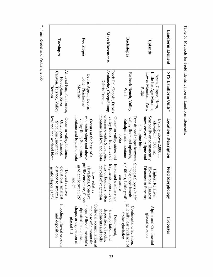
73
Table 5
. Meth
ods fo
r Field
Identificatio
n of L
andform
Elem
ents.
Landfo
rm E
lemen
t NPS L
andfo
rm U
nits*
Loca
tion / D
escriptio
n
Field
Morp
holo
gy
Pro
cesses
Upla
nds
Arete, C
irque, H
orn,
Little Ice A
ge M
orain
e,
Lower M
ountain
, Pass,
Ridge
Usually
above 2
,000 m
elevatio
n (±
500 m
),
Seaso
nally
or p
ermanently
snow co
vered
, Alip
ne an
d
subalp
ine b
iotia
Highest R
elative
Elev
ations, L
argest
Distan
ce to Stream
s
Alpine an
d Contin
ental
glacial ero
sion
Back
slopes
Bedrock Bench, V
alley
Wall
Tran
sitional slo
pe b
etween
valley
floor an
d uplan
ds,
Subalp
ine an
d m
ontan
e
biotia
Steep
est Slopes (>
25°),
long slo
pe len
gth
(>100 m
), Little p
rofile
curvatu
re
Contin
ental G
laciation,
generally
less evidence o
f
alpine g
laciation
Mass M
ovem
ents
Rock Fall/T
opple, D
ebris
Avalan
che, C
reep/Slump,
Debris T
oren
t,
Occu
r on valle
y sid
es and
valley
floors, E
vidence o
f
errosio
n ev
ents, S
ubalp
ine,
montan
e and lo
wlan
d biota
Increased
surface ro
ck
fragments, p
resence o
f
talus o
r boulders, o
ften
devoid of v
egetatio
n
Detach
ment,
transportatio
n an
d
depositio
n of ro
cks,
sedim
ents an
d so
ils
Footslo
pes
Debris A
pron, D
ebris
Cone, P
leistocen
e
Morain
e
Occu
rs at the b
ase of a
mountain
slope an
d ab
ove
valley
floor, S
ubalp
ine,
montan
e and lo
wlan
d biota
Low relativ
e
elevatio
ns, C
oncav
e
profile cu
rvatu
re, Slope
grad
ient b
etween
25°
and 5°
Collu
vial accu
mulatio
n at
the b
ase of a m
ountain
slope, A
lluvial m
aterials
dposited
in a co
nical
shape, o
r depositio
n of
glacial till
Toeslo
pes
Allu
vial F
an, F
an Terace,
Floodplain
, River
Canyon, T
errace, Valle
y
Botto
m
Occu
r in valle
y botto
ms,
Often
poorly
drain
ed,
Subalp
ine, m
ontan
e,
lowlan
d an
d wetlan
d biota
Lowest relativ
e
elevatio
ns, sm
allest
distan
ce to stream
s,
gentle slo
pes (<
5°)
Flooding, F
luvial ero
sion
and depositio
n
* From Ried
el and Probala, 2
005
74
landscape position. This was needed to prevent the majority of the cluster locations from falling
in valley bottoms, which generally have the largest variance in landform and land cover due to a
combination of alluvial and colluvial landforms. Originally, 100 cluster locations were chosen
using a spatial inhibition distance of 500 m between cluster centers. Many more sample
locations were selected than were needed; however, this allowed for flexibility to select sample
locations based on accessibility and safety. In total 25 clusters were sampled during 2007 and
2008. At each cluster, I collected landform observations from a central point and three points
along three separate transects (ten points per cluster). Along any given transect, points were
spaced at approximately 15, 45, and 150 m from the cluster center. Clusters were randomly
placed with one transect facing either north, south, east or west. Cluster centers were located in
the field with GPS. In total, I collected 429 site descriptions of landform class. Landform classes
were determined in the field according to their location within the landscape, morphological
characteristics and geomorphic processes.
Digital data layers were assembled into a GIS and a digital database was constructed
containing field observations. I acquired a 10 m spatial resolution digital elevation model
(DEM) from the United States Geologic Survey. Terrain attributes were calculated from the
DEM using spatial analysis tools within the ArcGIS software (ESRI, 2008). Predictor variables
included slope gradient (Burrough and Mc Donell, 1988), aspect of slope (Burrough and Mc
Donell, 1988), elevation, profile curvature (Moore et al., 1991; Zeverbergen and Thorne, 1987),
plan curvature (Moore et al., 1991; Zeverbergen and Thorne, 1987), wetness index (Tarboten et
al., 1991; Greenlee, 1987; Jenson and Domingue, 1988), horizontal and vertical distance to the
nearest stream (MacMillan et al., 2000), and stream order (Strahler, 1952) of the nearest stream.
75
I employed two methods of inductive classification to identify landforms based on DEM-
derived terrain attributes: (1) binary decision trees (BDT) and (2) random forest machine
learning (RF). These modeling approaches were implemented using the ‘rpart’ and
‘randomForest’ packages, respectively, in the R Project for Statistical Computing (R
development core team, 2008). Binary decision trees provide logical rules of classification by
seeking patterns within the data (Brieman et al., 1984). The BDT splits the data into landform
classes at specific values of a given terrain attribute. Decision trees identify important
relationships in the data and capture clusters of observations with similar landform types and
similar terrain attributes. Random forest is a form of machine learning in which classification
trees are iteratively fit to random sub-samples of the calibration data set (Brieman, 2001). Votes
are tallied from a large number of iterations (hundreds to thousands) to determine the predicted
class.
Using 409 field observations within the watershed boundaries, I compared the NPS
expert map to field observations. To accomplish objective 1, confusion matrices and the kappa
statistic were used to evaluate the existing NPS expert map. Field observations of landform
element were randomly split into calibration (n = 286) and validation (n = 143) data sets. To
ensure validation independence, all observations in a cluster were assigned as a whole to either
calibration or validation data sets. Confusion matrices and the kappa statistic were used to
evaluate the correlation between model predictions and field observations of landform elements,
thus achieving objective 2. Terrain attributes were calculated at every point in the watershed and
the resulting statistical models were then applied to map the study area. These maps were
evaluated by comparing them with the NPS expert map, digital photographs and three-
dimensional digital representations, realizing objective 3.

76
I selected 16 soil variables (categorical and continuous) and compared these with terrain
attributes and landform elements, achieving objective 4. Categorical soil variables included
taxonomic classification, soil occurrence, E-Bs horizon sequence presence/absence, volcanic
tephra occurrence and the presence or absence of redoxomorphic features. Categorical variables
were graphically compared with field observations of landform elements to discern soil-landform
relationships, partially achieving objective 5. Continuous soil variables included solum
thickness, organic horizon thickness, topsoil thickness, mineral surface percent total carbon,
mineral surface percent total nitrogen, mineral surface color (hue/value/chroma) and subsoil
color (hue/value/chroma). Continuous soil variables were modeled with generalized least
squares (GLS) regression. These analyses included checking and correcting for violations of
general regression assumptions, including normality, constant error variance and spatial
autocorrelation. In GLS, multiple models can be fit simultaneously. This allows us to model a
trend surface, a spatial correlation structure and a variance structure, as needed. Analysis of
variance was used to test the marginal significance of model components. For regression
modeling, observations were split into calibration and validation data sets using a 2/3 to 1/3 split.
To ensure validation independence, all observations in a cluster were assigned as a whole to
either calibration or validation data sets. GLS models were used to predict soil properties and
were compared with observed landform elements, completing objective 5. The ratios of standard
deviations of the validation data sets to the standard errors of prediction for the resulting models
are useful in evaluating GLS models. If this ratio has a value larger than 1, this indicates a given
model has reduced the error in estimates of soil properties. If the ratio is smaller than 1, it
indicates that these models do not provide accurate predictions for targeted soil variables.
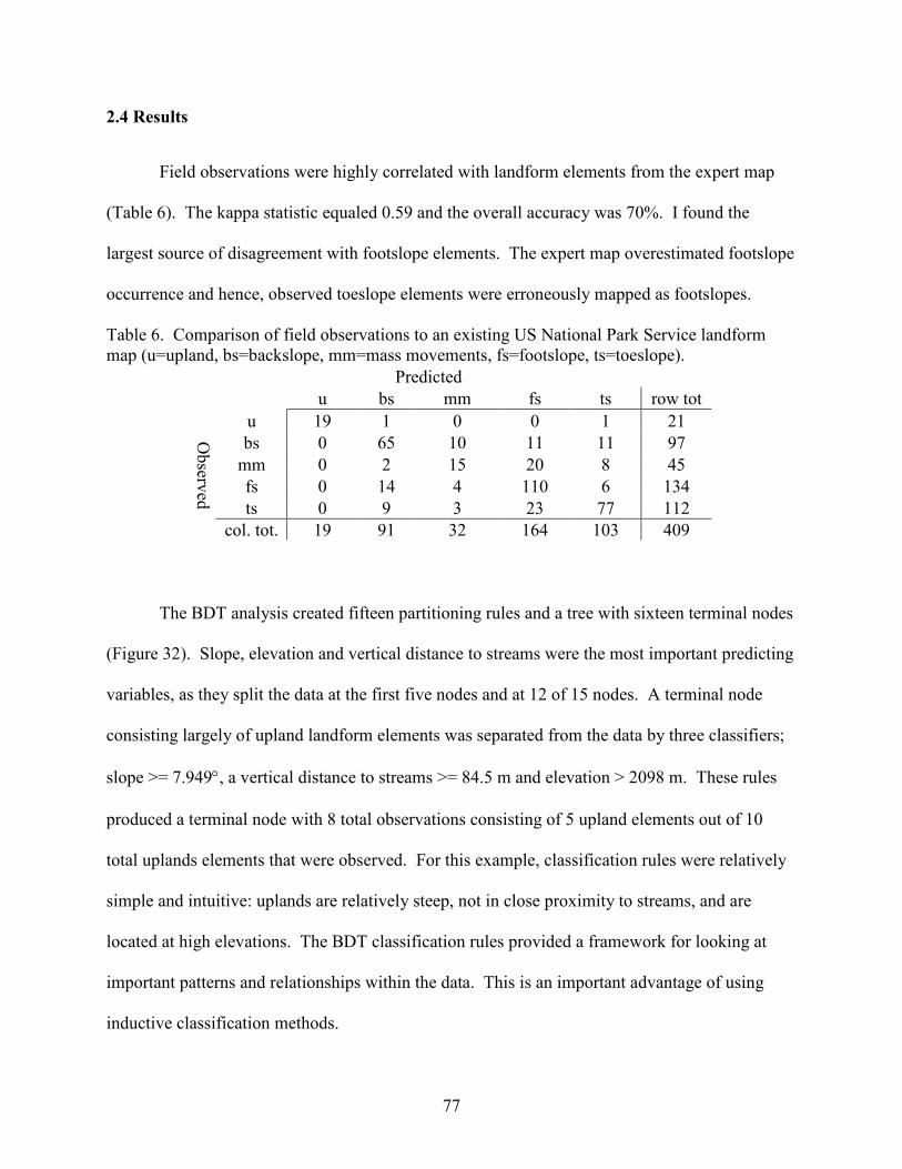
77
2.4 Results
Field observations were highly correlated with landform elements from the expert map
(Table 6). The kappa statistic equaled 0.59 and the overall accuracy was 70%. I found the
largest source of disagreement with footslope elements. The expert map overestimated footslope
occurrence and hence, observed toeslope elements were erroneously mapped as footslopes.
Table 6. Comparison of field observations to an existing US National Park Service landform
map (u=upland, bs=backslope, mm=mass movements, fs=footslope, ts=toeslope).
Predicted
u bs mm fs ts row tot
u 19 1 0 0 1 21
bs 0 65 10 11 11 97
mm 0 2 15 20 8 45
fs 0 14 4 110 6 134
ts 0 9 3 23 77 112
Observ
ed
col. tot. 19 91 32 164 103 409
The BDT analysis created fifteen partitioning rules and a tree with sixteen terminal nodes
(Figure 32). Slope, elevation and vertical distance to streams were the most important predicting
variables, as they split the data at the first five nodes and at 12 of 15 nodes. A terminal node
consisting largely of upland landform elements was separated from the data by three classifiers;
slope >= 7.949°, a vertical distance to streams >= 84.5 m and elevation > 2098 m. These rules
produced a terminal node with 8 total observations consisting of 5 upland elements out of 10
total uplands elements that were observed. For this example, classification rules were relatively
simple and intuitive: uplands are relatively steep, not in close proximity to streams, and are
located at high elevations. The BDT classification rules provided a framework for looking at
important patterns and relationships within the data. This is an important advantage of using
inductive classification methods.
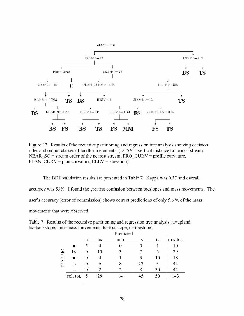
78
Figure 32. Results of the recursive partitioning and regression tree analysis showing decision
rules and output classes of landform elements. (DTSV = vertical distance to nearest stream,
NEAR_SO = stream order of the nearest stream, PRO_CURV = profile curvature,
PLAN_CURV = plan curvature, ELEV = elevation)
The BDT validation results are presented in Table 7. Kappa was 0.37 and overall
accuracy was 53%. I found the greatest confusion between toeslopes and mass movements. The
user’s accuracy (error of commission) shows correct predictions of only 5.6 % of the mass
movements that were observed.
Table 7. Results of the recursive partitioning and regression tree analysis (u=upland,
bs=backslope, mm=mass movements, fs=footslope, ts=toeslope).
Predicted
u bs mm fs ts row tot.
u 5 4 0 0 1 10
bs 0 13 3 7 6 29
mm 0 4 1 3 10 18
fs 0 6 8 27 3 44
Observ
ed
ts 0 2 2 8 30 42
col. tot. 5 29 14 45 50 143

79
The random forest method yielded improvements over the binary decision-tree model.
When comparing the predicted landform class from the random forest model to the validation
data, the kappa statistic was 0.45 and the overall accuracy was 59% (Table 8). As with BDTs, I
found poor results with mass movement prediction. The user’s accuracy (error of commission)
shows correct prediction of only 11% of the mass movements that were observed. Mass
movements were misclassified mainly as either footslopes or toeslopes, but the mass movement
elements showed improvement over the BDT analysis. Upland elements showed improvement
over the BDT analysis as well.
Table 8. Results of the random forest analysis (u=upland, bs=backslope, mm=mass movements,
fs=footslope, ts=toeslope).
Predicted
u bs mm fs ts row tot.
u 7 2 0 1 0 10
bs 0 14 1 10 4 29
mm 0 2 2 5 9 18
fs 0 5 2 34 3 44
Observ
ed
ts 0 1 0 13 28 42
col. tot. 7 24 5 63 44 143
While the RF approach does not yield direct rules for classification, it is possible to
extract the relative importance of predictors (Table 9). For backslope, footslope and mass
movements elements, slope and vertical distance to streams were most relevant. For classifying
toeslopes, slope and elevation were the most important predictors. For obvious reasons,
elevation was the most important variable for predicting upland distribution.
Resulting BDT and RF classification methods were used to map the entire watershed and
to compare the resulting maps to the expert landform map. Results of watershed mapping with
BDT are compared with the NPS expert map in Figure 33. Results of watershed mapping with
RF are compared with the NPS expert map in Figure 34. The digital maps correlate well with
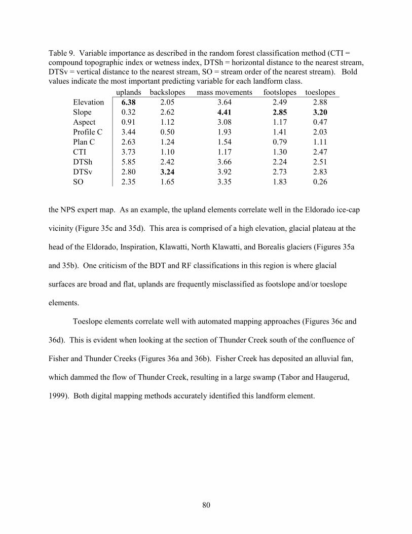
80
Table 9. Variable importance as described in the random forest classification method (CTI =
compound topographic index or wetness index, DTSh = horizontal distance to the nearest stream,
DTSv = vertical distance to the nearest stream, SO = stream order of the nearest stream). Bold
values indicate the most important predicting variable for each landform class.
uplands backslopes mass movements footslopes toeslopes
Elevation 6.38 2.05 3.64 2.49 2.88
Slope 0.32 2.62 4.41 2.85 3.20
Aspect 0.91 1.12 3.08 1.17 0.47
Profile C 3.44 0.50 1.93 1.41 2.03
Plan C 2.63 1.24 1.54 0.79 1.11
CTI 3.73 1.10 1.17 1.30 2.47
DTSh 5.85 2.42 3.66 2.24 2.51
DTSv 2.80 3.24 3.92 2.73 2.83
SO 2.35 1.65 3.35 1.83 0.26
the NPS expert map. As an example, the upland elements correlate well in the Eldorado ice-cap
vicinity (Figure 35c and 35d). This area is comprised of a high elevation, glacial plateau at the
head of the Eldorado, Inspiration, Klawatti, North Klawatti, and Borealis glaciers (Figures 35a
and 35b). One criticism of the BDT and RF classifications in this region is where glacial
surfaces are broad and flat, uplands are frequently misclassified as footslope and/or toeslope
elements.
Toeslope elements correlate well with automated mapping approaches (Figures 36c and
36d). This is evident when looking at the section of Thunder Creek south of the confluence of
Fisher and Thunder Creeks (Figures 36a and 36b). Fisher Creek has deposited an alluvial fan,
which dammed the flow of Thunder Creek, resulting in a large swamp (Tabor and Haugerud,
1999). Both digital mapping methods accurately identified this landform element.

81
Figure 33. Results of watershed mapping with binary decision trees (BDT) (uplands = yellow,
backslopes = green, mass movements = red, footslopes = blue, toeslopes = purple).
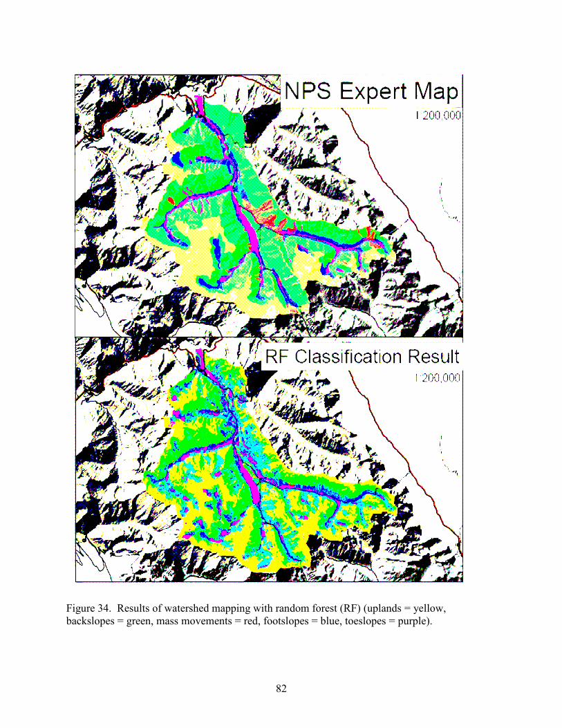
82
Figure 34. Results of watershed mapping with random forest (RF) (uplands = yellow,
backslopes = green, mass movements = red, footslopes = blue, toeslopes = purple).
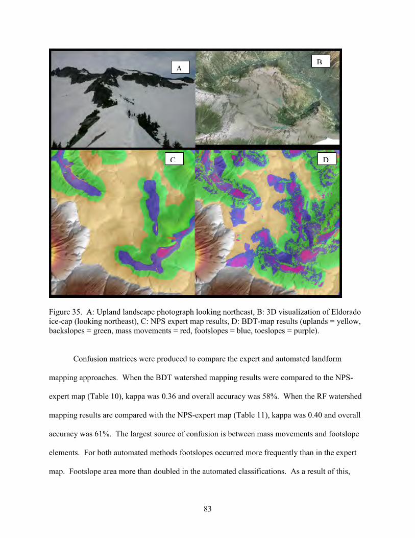
83
Figure 35. A: Upland landscape photograph looking northeast, B: 3D visualization of Eldorado
ice-cap (looking northeast), C: NPS expert map results, D: BDT-map results (uplands = yellow,
backslopes = green, mass movements = red, footslopes = blue, toeslopes = purple).
Confusion matrices were produced to compare the expert and automated landform
mapping approaches. When the BDT watershed mapping results were compared to the NPS-
expert map (Table 10), kappa was 0.36 and overall accuracy was 58%. When the RF watershed
mapping results are compared with the NPS-expert map (Table 11), kappa was 0.40 and overall
accuracy was 61%. The largest source of confusion is between mass movements and footslope
elements. For both automated methods footslopes occurred more frequently than in the expert
map. Footslope area more than doubled in the automated classifications. As a result of this,
D
B
C
A
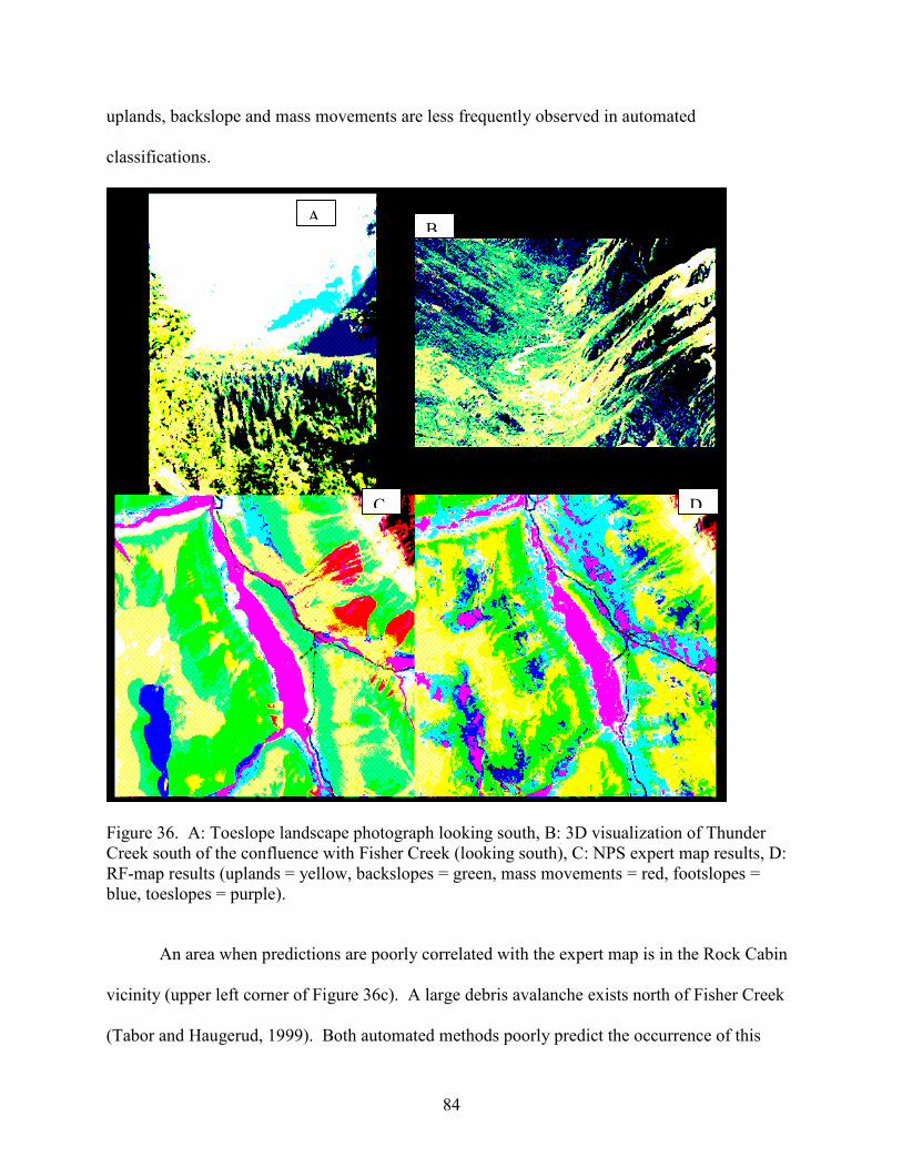
84
uplands, backslope and mass movements are less frequently observed in automated
classifications.
Figure 36. A: Toeslope landscape photograph looking south, B: 3D visualization of Thunder
Creek south of the confluence with Fisher Creek (looking south), C: NPS expert map results, D:
RF-map results (uplands = yellow, backslopes = green, mass movements = red, footslopes =
blue, toeslopes = purple).
An area when predictions are poorly correlated with the expert map is in the Rock Cabin
vicinity (upper left corner of Figure 36c). A large debris avalanche exists north of Fisher Creek
(Tabor and Haugerud, 1999). Both automated methods poorly predict the occurrence of this
B
D C
A
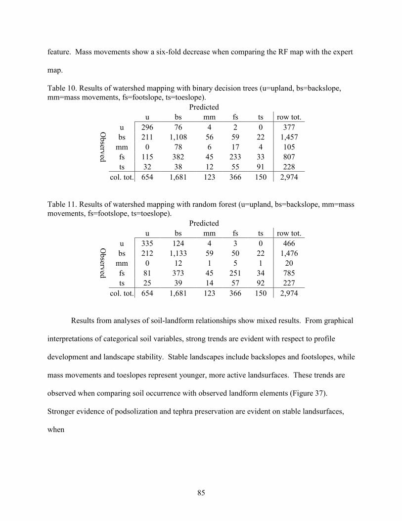
85
feature. Mass movements show a six-fold decrease when comparing the RF map with the expert
map.
Table 10. Results of watershed mapping with binary decision trees (u=upland, bs=backslope,
mm=mass movements, fs=footslope, ts=toeslope).
Predicted
u bs mm fs ts row tot.
u 296 76 4 2 0 377
bs 211 1,108 56 59 22 1,457
mm 0 78 6 17 4 105
fs 115 382 45 233 33 807
Observ
ed
ts 32 38 12 55 91 228
col. tot. 654 1,681 123 366 150 2,974
Table 11. Results of watershed mapping with random forest (u=upland, bs=backslope, mm=mass
movements, fs=footslope, ts=toeslope).
Predicted
u bs mm fs ts row tot.
u 335 124 4 3 0 466
bs 212 1,133 59 50 22 1,476
mm 0 12 1 5 1 20
fs 81 373 45 251 34 785
Observ
ed
ts 25 39 14 57 92 227
col. tot. 654 1,681 123 366 150 2,974
Results from analyses of soil-landform relationships show mixed results. From graphical
interpretations of categorical soil variables, strong trends are evident with respect to profile
development and landscape stability. Stable landscapes include backslopes and footslopes, while
mass movements and toeslopes represent younger, more active landsurfaces. These trends are
observed when comparing soil occurrence with observed landform elements (Figure 37).
Stronger evidence of podsolization and tephra preservation are evident on stable landsurfaces,
when
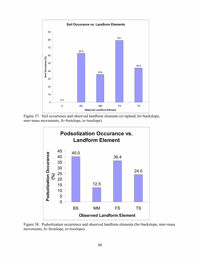
86
Figure 37. Soil occurrence and observed landform elements (u=upland, bs=backslope,
mm=mass movements, fs=footslope, ts=toeslope).
Figure 38. Podsolization occurrence and observed landform elements (bs=backslope, mm=mass
movements, fs=footslope, ts=toeslope).
Soil Occurance vs. Landform Elements
0.0
62.5
35.6
79.1
43.9
0
10
20
30
40
50
60
70
80
90
U BS MM FS TS
Observed Landform Element
Soil O
ccurance (%)
Podsolization Occurance vs.
Landform Element
40.0
12.5
36.4
24.0
0
5
10
15
20
25
30
35
40
45
BS MM FS TS
Observed Landform Element
Podsolization O
ccurance
(%)

87
Figure 39. Volcanic tephra occurrence and observed landform elements (bs=backslope,
mm=mass movements, fs=footslope, ts=toeslope).
Figure 40. Occurrence of redoxomorphic features and observed landform elements
(bs=backslope, mm=mass movements, fs=footslope, ts=toeslope).
Ash Occurance vs. Landform Elements
78.3
43.8
74.5
38.0
0
10
20
30
40
50
60
70
80
90
BS MM FS TS
Observed Landform Element
Ash O
ccurance (%)
Redox Occurance vs. Landform Elements
4.3
14.3
9.0
67.6
0
10
20
30
40
50
60
70
80
BS MM FS TS
Observed Landform Element
Redox O
ccurance (%)

88
Figure 41. Distribution of soil orders with respect to landform elements (bs=backslope,
mm=mass movements, fs=footslope, ts=toeslope).
compared to active landsurfaces (Figures 38 and 39). Redoxomorphic features are highly
correlated with toeslope landform elements (Figure 40). Landscape stability trends are also
reflected in the classification of these soils (Figure 41). Stable landsurfaces support a greater
number of Spodosols and Andisols, while active landsurface are dominated by Entisols,
Inceptisols and Histosols.
When comparing continuous soil variables with terrain attributes and landform elements,
less correlation exists (Table 12). Generalized least squares regression models are highly
significant yet provide poor predictions of soil properties. The ratios of standard deviations of
the validation data sets to the standard errors of prediction for the resulting GLS models are near
Soil Orders and Landform Elements
13
1 09
63
10
45
12
0
23
25
40
13
34
6
40
13
3324
00%
10%
20%
30%
40%
50%
60%
70%
80%
90%
100%
BS MM FS TS
Observed Landform Element
Soil O
rder
(% of observations)
Histosols Entisols Inceptisols Andisols Spodosols
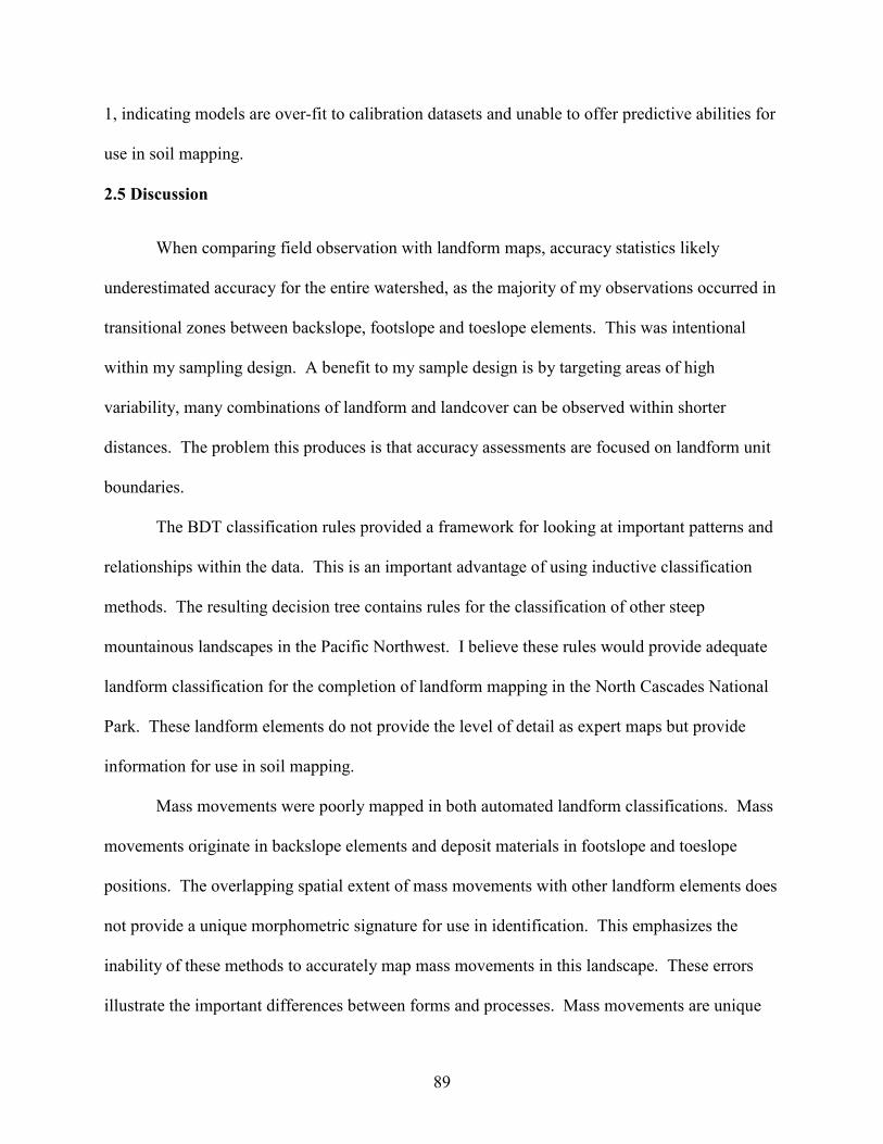
89
1, indicating models are over-fit to calibration datasets and unable to offer predictive abilities for
use in soil mapping.
2.5 Discussion
When comparing field observation with landform maps, accuracy statistics likely
underestimated accuracy for the entire watershed, as the majority of my observations occurred in
transitional zones between backslope, footslope and toeslope elements. This was intentional
within my sampling design. A benefit to my sample design is by targeting areas of high
variability, many combinations of landform and landcover can be observed within shorter
distances. The problem this produces is that accuracy assessments are focused on landform unit
boundaries.
The BDT classification rules provided a framework for looking at important patterns and
relationships within the data. This is an important advantage of using inductive classification
methods. The resulting decision tree contains rules for the classification of other steep
mountainous landscapes in the Pacific Northwest. I believe these rules would provide adequate
landform classification for the completion of landform mapping in the North Cascades National
Park. These landform elements do not provide the level of detail as expert maps but provide
information for use in soil mapping.
Mass movements were poorly mapped in both automated landform classifications. Mass
movements originate in backslope elements and deposit materials in footslope and toeslope
positions. The overlapping spatial extent of mass movements with other landform elements does
not provide a unique morphometric signature for use in identification. This emphasizes the
inability of these methods to accurately map mass movements in this landscape. These errors
illustrate the important differences between forms and processes. Mass movements are unique
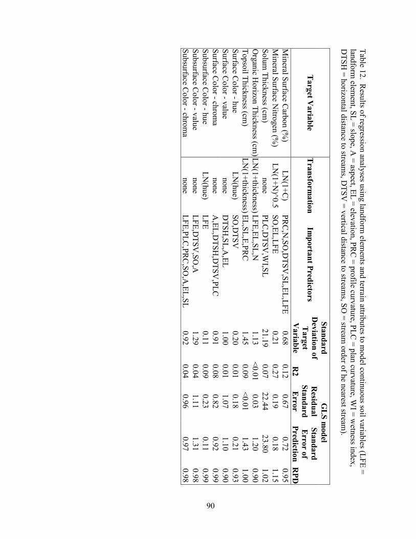
90
Table 1
2. R
esults o
f regressio
n an
alyses u
sing lan
dform
elements an
d terrain
attributes to
model co
ntin
uous so
il variab
les (LFE =
landform
element, S
L = slo
pe, A
= asp
ect, EL = elev
ation, P
RC = profile cu
rvatu
re, PLC = plan
curvatu
re, WI =
wetn
ess index,
DTSH = horizo
ntal d
istance to
streams, D
TSV = vertical d
istance to
streams, S
O = stream
order o
f he n
earest stream).
GLS m
odel
Targ
et Varia
ble
Tra
nsfo
rmatio
n
Importa
nt P
redicto
rs
Sta
ndard
Dev
iatio
n of
Targ
et
Varia
ble
R2
Resid
ual
Sta
ndard
Erro
r
Sta
ndard
Erro
r of
Pred
iction RPD
Mineral S
urface C
arbon (%
) LN(1+C)
PRC,N,SO,DTSV,SL,EL,LFE
0.68
0.12
0.67
0.72
0.95
Mineral S
urface N
itrogen (%
) LN(1+N)^0.5 SO,EL,LFE
0.21
0.27
0.19
0.18
1.15
Solum Thick
ness (cm
) none
PLC,DTSV,W
I,SL
21.19
0.07
22.44
23.80
1.02
Organic H
orizo
n Thick
ness (cm
) LN(1+thick
ness) L
FE,EL,SL,N
1.13
<0.01
0.03
1.20
0.90
Topsoil T
hick
ness (cm
) LN(1+thick
ness) E
L,SL,E,PRC
1.45
0.09
<0.01
1.43
1.00
Surface C
olor - h
ue
LN(hue)
SO,DTSV
0.20
0.01
0.18
0.21
0.93
Surface C
olor - v
alue
none
DTSH,SL,A,EL
1.00
0.01
1.07
1.10
0.90
Surface C
olor - ch
roma
none
A,EL,DTSH,DTSV,PLC
0.91
0.08
0.82
0.92
0.99
Subsurface C
olor - h
ue
LN(hue)
LFE
0.11
0.09
0.23
0.11
0.99
Subsurface C
olor - v
alue
none
LFE,DTSV,SO,A
1.29
0.04
1.11
1.31
0.98
Subsurface C
olor - ch
roma
none
LFE,PLC,PRC,SO,A,EL,SL
0.92
0.04
0.96
0.97
0.98

91
from the other landform elements in this work because they are describing a process and not
surficial morphology alone. Automated methods rely on form to infer process. Poor prediction
of mass movements illustrates how tacit assumptions between form and process are very
important when automatically mapping landforms from remotely sensed data. The nine selected
terrain attributes failed to accurately identify morphometric characteristics to differentiate mass
movements from other landform elements. The process of mass wasting is not readily identified
by form alone, in this work. This problem may be overcome by using more terrain attributes but
remains a limitation.
Relative position indices like horizontal and vertical distance to streams provided more
information than measures of curvature or wetness. Overall, slope was the most important
terrain attribute for this modeling exercise. By adjusting the size of the area used to calculate
curvature, these terrain attributes may become more useful. A study designed to optimize terrain
attributes for use in soil and landform mapping is necessary.
Although soil property maps are easily created with GIS software they have little
relevance to the spatial distributions of soil characteristics. I hypothesize two potential issues
that render advanced statistical inferences inappropriate. First, the geographic distribution of soil
properties (carbon content, solum thickness, soil color) is highly variable across the landscape,
and secondly, the scale of spatial variability is not described by 4th order soil surveys, nor is it
intended to.
A question I must address in digital mapping and modeling is the issue of scale. Scale
controls the size of maps but also the size and resolution of geospatial data, computation
processing speeds, and level of detail for describing soils. Soil surveys produced for this region
frequently rely on complexes, consociations, and associations when characterizing soils (Rogers,

92
2000; Briggs, 2004). These complex soil map units are needed to describe the spatial variability
in the distribution of soil properties and classes. When seeking statistical relationships for
comparison of soils and topography, one adjusts the analyses according to scale; similarly to the
way one adapts soil mapping units to site specific mapping needs. At the level of detail used in
this research, graphical representations of broader soil landscape trends are more useful than
regression analyses of continuous soil variables. Soil physical and chemical properties are not
accurately predicted within the scale of these models. Denser sampling and higher resolution
spatial data may achieve this.
2.6 Conclusions
For this study, automated landform mapping in humid, mountainous terrain approached
the accuracy of an expert, National Park Service landform map. Field observations of landforms
correlated well with the expert landform map (kappa = 0.59 and overall accuracy = 70%).
Comparing the two automated methods, the random forest classification (kappa = 0.45 and
overall accuracy = 59%) performed better than the binary decision tree method (kappa = 0.37
and overall accuracy = 53%). Observations were focused on zones of transition between
landform elements; therefore I likely underestimated the accuracy of these methods for
classifying the whole watershed. Watershed mapping with automated methods shows good
correlation with expert maps, however mass movements were poorly correlated. This highlights
a limitation of automated mapping with remotely sensed data. Morphometrics cannot directly
describe processes that produce landforms, and are limited solely to describing the form of the
land surface.
Overall, slope and vertical distance to streams were the most important predictor for both
the BDT and RF classification models. Elevation was important for distinguishing upland areas.

93
Distances to stream (horizontal and vertical) were important predictors while measures of
curvature and wetness were less useful. Optimization of the window size used for the calculation
of terrain attributes may offer improved landform classifications and predictions of soil
properties.
Soil-landform relationships are questions by these results. When mapping soils, an
independent, explicit and quantitative test of a surveyor’s mental model in required to provide
knowledge of data quality. This is frequently lacking (Hudson, 1992). Digital soil mapping
increases the opportunities for assessing the accuracy of soil mapping tenants. If terrain
attributes and landform elements are not correlated with profile characteristics, one must look
elsewhere for tools to characterize soil properties (Jenny, 1941). Soil profile characteristics
show stronger correlations when compared with vegetation and biological characteristics in soils
of the North Cascades (Meirik, 2008).
Future work should apply digital landform maps in combination with remotely sensed
maps of land cover to digitally map soils in the watershed. Should higher resolution DEM data
become available, it would be interesting to examine the effects of DEM spatial resolution and
error on landform classification and soil mapping.
2.7 Acknowledgements
I would like to thank USDA – NGDC for funding this work. I would like to thank the
NPS for allowing this research to take place. Also, NPS geologist Jon Riedel helped me to
understand the landforms in TCW. Finally, US Department of Agriculture – Natural Resource
Conservation Service Staff Toby Rodgers and Crystal Briggs have helped greatly in
understanding the soils of the region.
94
2.8 References
Bolongaro-Crevenna, A., Torres-Rodriguez, V., Sorani, V., Frame, D., and Ortiz, M.A. 2005.
Geomorphometric analysis for characterizing landforms in Morelos State, Mexico.
Geomorphology. 67:407-422.
Breiman, L., Friedman, J., Olshen, R., and Stone, C. 1984. Classification and regression trees.
Chapman and Hall/CRC, Boca Raton, FL.
Breiman, L. 2001. Random Forests. Machine Learning 45:5-32.
Briggs, C.A.D., Busacca, A.J. and McDaniel, P.A. 2006. Pedogenic processes and soil-
landscape relationships in North Cascades National Park, Washington. Geoderma 137:192-
204.
Burrough, P.A. and McDonell, R.A. 1988. Principles of geographical information systems.
Oxford University Press, New York. p. 190.
Conacher, A.J. and Dalrymple, J.B. 1977. The nine-unit landsurface model: An approach to
pedogeomorphic research. Geoderma 18:1-154.
Dobos, E., Micheli, E., Baumgardner, M.F., Biehl, L and Helt, T. 2000. Use of combined
digital elevation model and satellite radiometric data for regional soil mapping. Geoderma
97:367-391.
Ehsani, A.H., and Quiel, F. 2008. Geomorphometric feature analysis using morphometric
parameterization and artificial neural networks. Geomorphology. 99:1-12.
Environmental Systems Research Institute (ESRI). 2008. ArcGIS version 9.2. Redlands,
California.
Gessler, P.E., O.A. Chadwick, F. Chamran, L. Althouse and K. Holmes. 2000. Modeling soil-
landscape and ecosystem properties using terrain attributes. Soil Science Society of America
Journal 64:2046-2056.
Greenlee, D.D. 1987. Raster and vector processing for scanned linework. Photogrammetric
Engineering and Remote Sensing 53:1383-1387.
Hansen, M.K, D.J. Brown, P.E. Dennison, S.A. Graves and R.S. Bricklemyer. 2009.
Inductively mapping expert-derived soil-landscape units within dambo wetland catenae using
multispectral and topographic data. Geoderma 150:72-84.
Hengl, T., and Rossiter, D.G. 2003. Supervised landform classification to enhance and replace
photo-interpretation in semi-detailed soil survey. Soil Science Society of America Journal
67:1810-1822.
95
Hudson, B.D. 1992. The soil survey as a paradigm-based science. Soil Science Society of
America Journal 56:836-841.
Irving, B.J., Ventura, S.J., and Slater, B.K. 1997. Fuzzy and isodata classification of landform
elements from digital terrain data in Pleasant Valley, Wisconsin. Geoderma. 77:137-154.
Jenny, H. 1941. Factors of Soil Formation. McGraw Hill. New York, New York.
Jenson, S.K. and J.O. Domingue. 1988. Extracting topographic structure from digital elevation
data for geographic information system analysis. Photogrammetric Engineering and Remote
Sensing 54:1593-1600.
MacMillan, R.A., Pettapiece, W.W., Nolan, S.C., and Goddard, T.W. 2000. A generic
procedure for automatically segmenting landforms into landform elements using DEMs,
heuristic rules and fuzzy logic. Fuzzy Sets and Systems. 113:81-109.
MacMillan, R.A., D.E. Moon and R.A. Coupe. 2007. Automated predictive ecological mapping
in a forested region of B.C., Canada, 2001-2005. Geoderma 140:353-373.
McBratney, A.B., Mendonca-Santos, M.L., and Minasny, B. 2003. On digital soil mapping.
Geoderma 117:3-52.
Meirik, E.E. 2008. Mapping vegetation with remote sensing and analysis of soil-vegetation
interactions in North Cascades National Park, WA. Washington State University M.S.
Thesis.
Milne, G. 1935. Some suggested units for classification and mapping, particularly for East
African soils. Soil Resources 4:183-198.
Moore, I.D., Grayson, R.B., and Landson, A.R. 1991. Digital terrain modeling: A review of
hydrological, geomorphological and biological applications. Hydrological Processes 5:3-30.
Moore, I.D., P.E. Gessler, G.A. Nielsen and G.A. Peterson. 1993. Soil attribute prediction using
terrain analysis. Soil Science Society of America Journal 57:443-452.
Park, S.J., McSweeney, K. and Lowery, B. 2001. Identification of the spatial distribution of
soils using a process-based terrain characterization. Geoderma 103:249-272.
Pennock, D.J., Zebarth, B.J., and De Jong, E. 1987. Landform classification and soil
distribution in hummocky terrain, Saskatchewan, Canada. Geoderma 40:297-315.
R Development Core Team. 2008. R: A Language and Environment for Statistical Computing.
R Foundation for Statistical Computing. Vienna, Austria.
Riedel, J. and Probala, J. 2005. Mapping ecosystems at the landform scale in Washington State.
Park Science 23:37-42.
96
Rodgers, T.M. 2000. Modeling soils of the Sawtooth and Pasayten Wilderness areas with a GIS.
Washington State University M.S. Thesis.
Ruhe. R.V. 1961. Elements of the soil landscape. Transactions of the 7th International Congress
of Soil Science 4:165-169.
Saadat, H., Bonnell, R., Sharifi, F., Mehuys, G., Namdar, M., and Ale-Ebrahim, S. 2008.
Landform classification from a digital elevation model and satellite imagery.
Geomorphology. 100:453-464.
Schmidt, J. and Hewitt, A. 2004. Fuzzy land element classification from DTMs based on
geometry and terrain position. Geoderma 121:243-256.
Scull, P., Franklin, J., Chadwick, O.A. and McArthur, D. 2003. Predictive soil mapping: a
review. Progress in Physical Geography 27:171-197.
Strahler, A. N. 1952. Hypsometric (area altitude) analysis of erosional topology. Geological
Society of America Bulletin 63:1117-1142.
Tabor, R and R. Haugerud. 1999. Geology of the North Cascades; A Mountain Mosaic. Seattle,
Washington.
Tarboton, D.G., R.L. Bras, I. Rodriguez-Iturbe. 1991. On the extraction of channel networks
from digital elevation data. Hydrological Processes 5:81-100.
van Asselen, S., and Seijmonsbergen, A.C. 2006. Expert-driven semi-automated
geomorphological mapping for a mountainous area using a laser DTM. Geomorphology.
78:309-320.
Wilson, J.P. and Gallant, J.C. (eds.) 2000. Terrain analysis; Principles and applications. John
Wiley and Sons, New York, New York.
Western Regional Climate Center (WRCC) website http://www.wrcc.dri.edu/ Accessed January
21, 2009.
Zeverbergen, L.W. and Thorne, C.R. 1987. Quantitative analysis of land surface topography.
Earth Surface Processes and Landforms 12:47-56.
Ziadat, F.M. 2005. Analyzing digital terrain attributes to predict soil attributes for a relatively
large area. Soil Science Society of America Journal 69:1590-1599.

APPENDIX A
NATIONAL PARK SERVICE LANDFORM UNIT DESCRIPTIONS
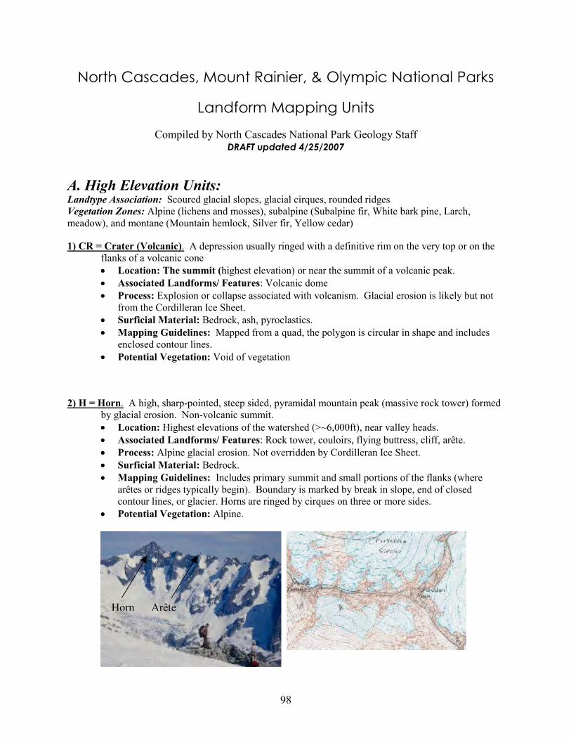
98
North Cascades, Mount Rainier, & Olympic National Parks
Landform Mapping Units
Compiled by North Cascades National Park Geology Staff DRAFT updated 4/25/2007
A. High Elevation Units: Landtype Association: Scoured glacial slopes, glacial cirques, rounded ridges
Vegetation Zones: Alpine (lichens and mosses), subalpine (Subalpine fir, White bark pine, Larch,
meadow), and montane (Mountain hemlock, Silver fir, Yellow cedar)
1) CR = Crater (Volcanic). A depression usually ringed with a definitive rim on the very top or on the
flanks of a volcanic cone
• Location: The summit (highest elevation) or near the summit of a volcanic peak.
• Associated Landforms/ Features: Volcanic dome
• Process: Explosion or collapse associated with volcanism. Glacial erosion is likely but not
from the Cordilleran Ice Sheet.
• Surficial Material: Bedrock, ash, pyroclastics.
• Mapping Guidelines: Mapped from a quad, the polygon is circular in shape and includes
enclosed contour lines.
• Potential Vegetation: Void of vegetation
2) H = Horn. A high, sharp-pointed, steep sided, pyramidal mountain peak (massive rock tower) formed
by glacial erosion. Non-volcanic summit.
• Location: Highest elevations of the watershed (>~6,000ft), near valley heads.
• Associated Landforms/ Features: Rock tower, couloirs, flying buttress, cliff, arête.
• Process: Alpine glacial erosion. Not overridden by Cordilleran Ice Sheet.
• Surficial Material: Bedrock.
• Mapping Guidelines: Includes primary summit and small portions of the flanks (where
arêtes or ridges typically begin). Boundary is marked by break in slope, end of closed
contour lines, or glacier. Horns are ringed by cirques on three or more sides.
• Potential Vegetation: Alpine.
Horn Arête
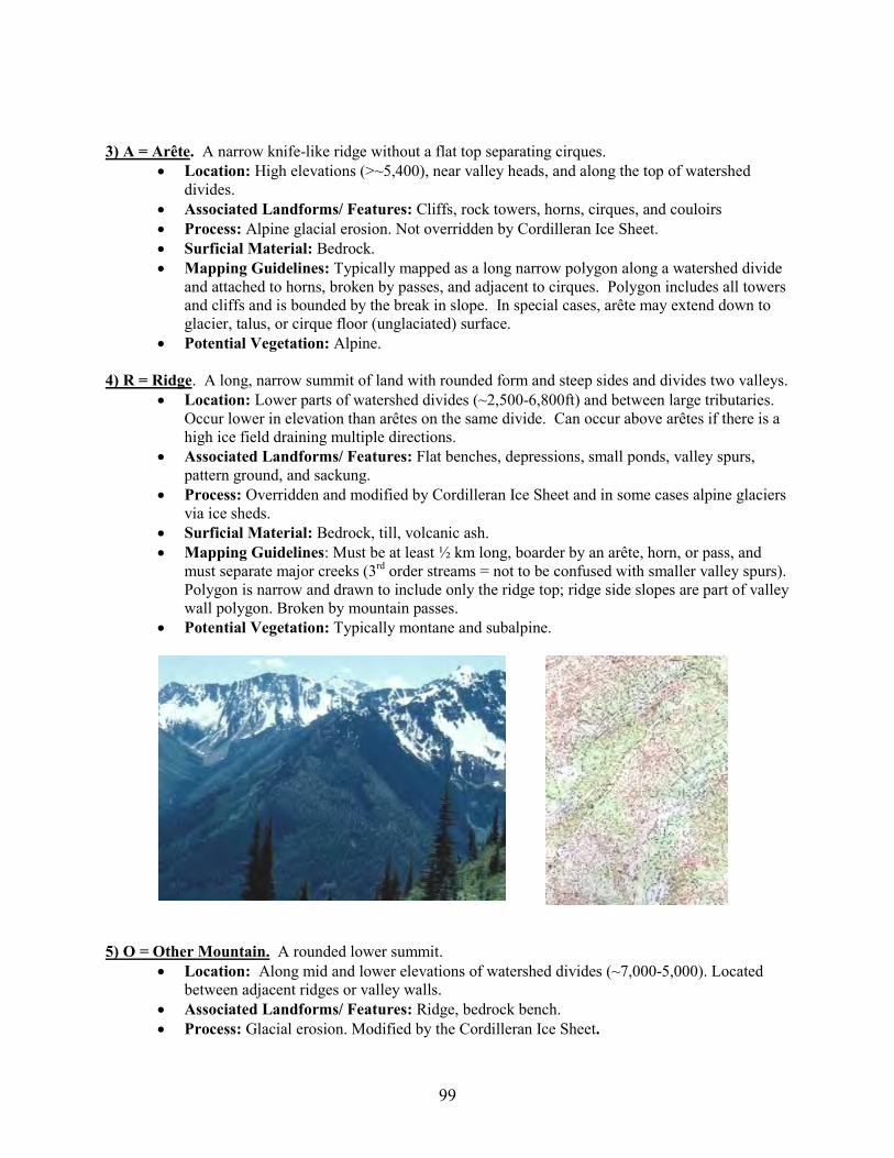
99
3) A = Arête. A narrow knife-like ridge without a flat top separating cirques.
• Location: High elevations (>~5,400), near valley heads, and along the top of watershed
divides.
• Associated Landforms/ Features: Cliffs, rock towers, horns, cirques, and couloirs
• Process: Alpine glacial erosion. Not overridden by Cordilleran Ice Sheet.
• Surficial Material: Bedrock.
• Mapping Guidelines: Typically mapped as a long narrow polygon along a watershed divide
and attached to horns, broken by passes, and adjacent to cirques. Polygon includes all towers
and cliffs and is bounded by the break in slope. In special cases, arête may extend down to
glacier, talus, or cirque floor (unglaciated) surface.
• Potential Vegetation: Alpine.
4) R = Ridge. A long, narrow summit of land with rounded form and steep sides and divides two valleys.
• Location: Lower parts of watershed divides (~2,500-6,800ft) and between large tributaries.
Occur lower in elevation than arêtes on the same divide. Can occur above arêtes if there is a
high ice field draining multiple directions.
• Associated Landforms/ Features: Flat benches, depressions, small ponds, valley spurs,
pattern ground, and sackung.
• Process: Overridden and modified by Cordilleran Ice Sheet and in some cases alpine glaciers
via ice sheds.
• Surficial Material: Bedrock, till, volcanic ash.
• Mapping Guidelines: Must be at least ½ km long, boarder by an arête, horn, or pass, and
must separate major creeks (3rd order streams = not to be confused with smaller valley spurs).
Polygon is narrow and drawn to include only the ridge top; ridge side slopes are part of valley
wall polygon. Broken by mountain passes.
• Potential Vegetation: Typically montane and subalpine.
5) O = Other Mountain. A rounded lower summit.
• Location: Along mid and lower elevations of watershed divides (~7,000-5,000). Located
between adjacent ridges or valley walls.
• Associated Landforms/ Features: Ridge, bedrock bench.
• Process: Glacial erosion. Modified by the Cordilleran Ice Sheet.
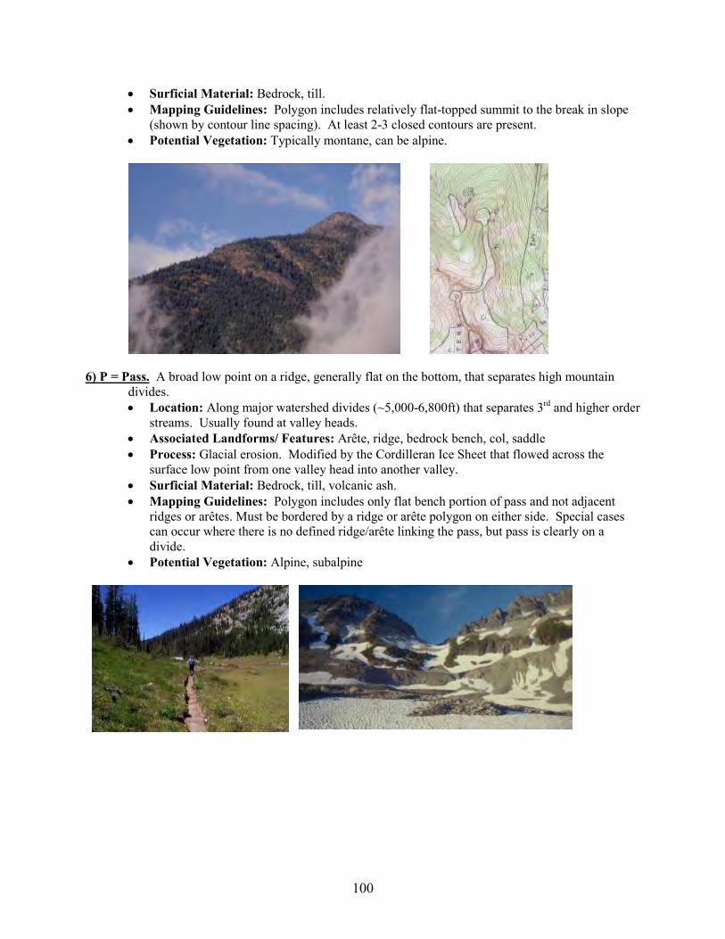
100
• Surficial Material: Bedrock, till.
• Mapping Guidelines: Polygon includes relatively flat-topped summit to the break in slope
(shown by contour line spacing). At least 2-3 closed contours are present.
• Potential Vegetation: Typically montane, can be alpine.
6) P = Pass. A broad low point on a ridge, generally flat on the bottom, that separates high mountain
divides.
• Location: Along major watershed divides (~5,000-6,800ft) that separates 3rd and higher order
streams. Usually found at valley heads.
• Associated Landforms/ Features: Arête, ridge, bedrock bench, col, saddle
• Process: Glacial erosion. Modified by the Cordilleran Ice Sheet that flowed across the
surface low point from one valley head into another valley.
• Surficial Material: Bedrock, till, volcanic ash.
• Mapping Guidelines: Polygon includes only flat bench portion of pass and not adjacent
ridges or arêtes. Must be bordered by a ridge or arête polygon on either side. Special cases
can occur where there is no defined ridge/arête linking the pass, but pass is clearly on a
divide.
• Potential Vegetation: Alpine, subalpine
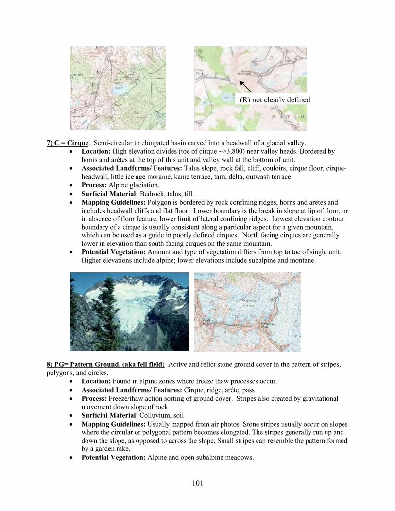
101
7) C = Cirque. Semi-circular to elongated basin carved into a headwall of a glacial valley.
• Location: High elevation divides (toe of cirque ~>3,800) near valley heads. Bordered by
horns and arêtes at the top of this unit and valley wall at the bottom of unit.
• Associated Landforms/ Features: Talus slope, rock fall, cliff, couloirs, cirque floor, cirque-
headwall, little ice age moraine, kame terrace, tarn, delta, outwash terrace
• Process: Alpine glaciation.
• Surficial Material: Bedrock, talus, till.
• Mapping Guidelines: Polygon is bordered by rock confining ridges, horns and arêtes and
includes headwall cliffs and flat floor. Lower boundary is the break in slope at lip of floor, or
in absence of floor feature, lower limit of lateral confining ridges. Lowest elevation contour
boundary of a cirque is usually consistent along a particular aspect for a given mountain,
which can be used as a guide in poorly defined cirques. North facing cirques are generally
lower in elevation than south facing cirques on the same mountain.
• Potential Vegetation: Amount and type of vegetation differs from top to toe of single unit.
Higher elevations include alpine; lower elevations include subalpine and montane.
8) PG= Pattern Ground. (aka fell field) Active and relict stone ground cover in the pattern of stripes,
polygons, and circles.
• Location: Found in alpine zones where freeze thaw processes occur.
• Associated Landforms/ Features: Cirque, ridge, arête, pass
• Process: Freeze/thaw action sorting of ground cover. Stripes also created by gravitational
movement down slope of rock
• Surficial Material: Colluvium, soil
• Mapping Guidelines: Usually mapped from air photos. Stone stripes usually occur on slopes
where the circular or polygonal pattern becomes elongated. The stripes generally run up and
down the slope, as opposed to across the slope. Small stripes can resemble the pattern formed
by a garden rake.
• Potential Vegetation: Alpine and open subalpine meadows.
(R) not clearly defined
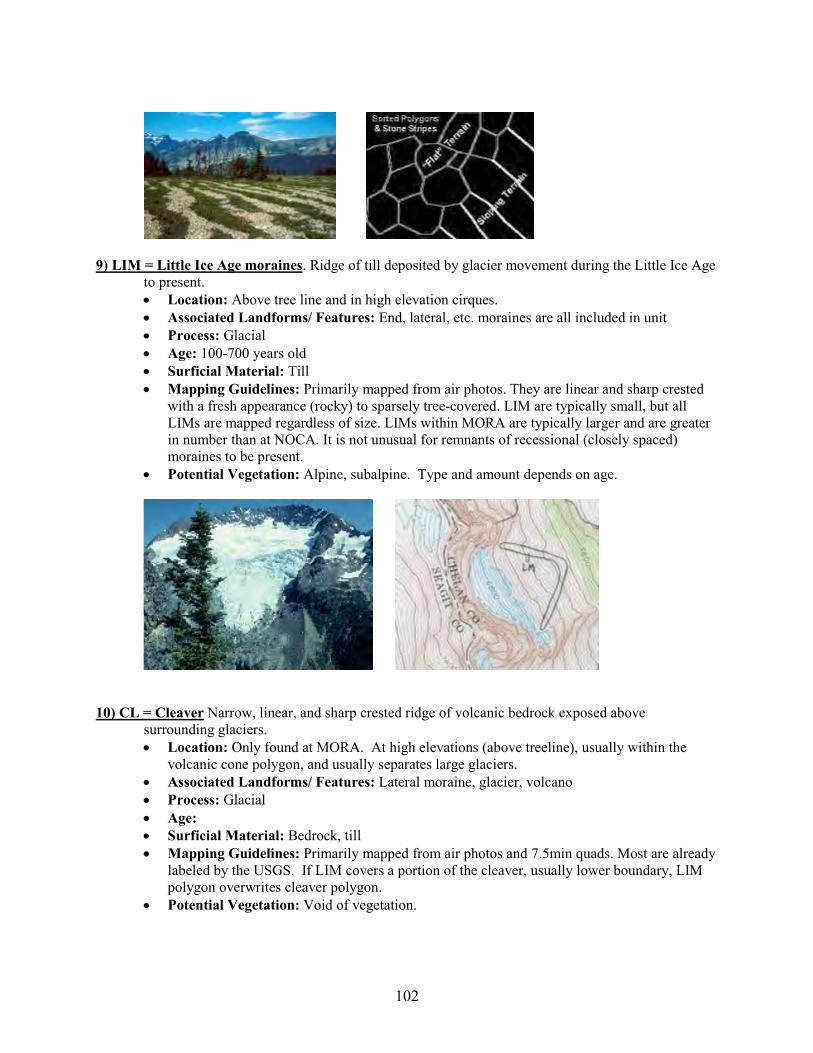
102
9) LIM = Little Ice Age moraines. Ridge of till deposited by glacier movement during the Little Ice Age
to present.
• Location: Above tree line and in high elevation cirques.
• Associated Landforms/ Features: End, lateral, etc. moraines are all included in unit
• Process: Glacial
• Age: 100-700 years old
• Surficial Material: Till
• Mapping Guidelines: Primarily mapped from air photos. They are linear and sharp crested
with a fresh appearance (rocky) to sparsely tree-covered. LIM are typically small, but all
LIMs are mapped regardless of size. LIMs within MORA are typically larger and are greater
in number than at NOCA. It is not unusual for remnants of recessional (closely spaced)
moraines to be present.
• Potential Vegetation: Alpine, subalpine. Type and amount depends on age.
10) CL = Cleaver Narrow, linear, and sharp crested ridge of volcanic bedrock exposed above
surrounding glaciers.
• Location: Only found at MORA. At high elevations (above treeline), usually within the
volcanic cone polygon, and usually separates large glaciers.
• Associated Landforms/ Features: Lateral moraine, glacier, volcano
• Process: Glacial
• Age:
• Surficial Material: Bedrock, till
• Mapping Guidelines: Primarily mapped from air photos and 7.5min quads. Most are already
labeled by the USGS. If LIM covers a portion of the cleaver, usually lower boundary, LIM
polygon overwrites cleaver polygon.
• Potential Vegetation: Void of vegetation.
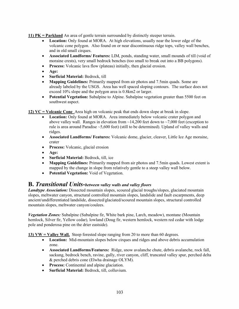
103
11) PK = Parkland An area of gentle terrain surrounded by distinctly steeper terrain.
• Location: Only found at MORA. At high elevations, usually near the lower edge of the
volcanic cone polygon. Also found on or near discontinuous ridge tops, valley wall benches,
and in old small cirques.
• Associated Landforms/ Features: LIM, ponds, standing water, small mounds of till (void of
moraine crests), very small bedrock benches (too small to break out into a BB polygons).
• Process: Volcanic lava flow (plateau) initially, then glacial erosion.
• Age:
• Surficial Material: Bedrock, till
• Mapping Guidelines: Primarily mapped from air photos and 7.5min quads. Some are
already labeled by the USGS. Area has well spaced sloping contours. The surface does not
exceed 10% slope and the polygon area is 0.8km2 or larger.
• Potential Vegetation: Subalpine to Alpine. Subalpine vegetation greater than 5500 feet on
southwest aspect.
12) VC = Volcanic Cone Area high on volcanic peak that ends down slope at break in slope.
• Location: Only found at MORA. Area immediately below volcanic crater polygon and
above valley wall. Ranges in elevation from ~14,200 feet down to ~7,000 feet (exception to
rule is area around Paradise ~5,600 feet) (still to be determined). Upland of valley walls and
ridges.
• Associated Landforms/ Features: Volcanic dome, glacier, cleaver, Little Ice Age moraine,
crater
• Process: Volcanic, glacial erosion
• Age:
• Surficial Material: Bedrock, till, ice
• Mapping Guidelines: Primarily mapped from air photos and 7.5min quads. Lowest extent is
mapped by the change in slope from relatively gentle to a steep valley wall below.
• Potential Vegetation: Void of Vegetation.
B. Transitional Units-between valley walls and valley floors Landtype Association: Dissected mountain slopes, scoured glacial troughs/slopes, glaciated mountain
slopes, meltwater canyon, structural controlled mountain slopes, landslide and fault escarpments, deep
ancient/undifferentiated landslide, dissected/glaciated/scoured mountain slopes, structural controlled
mountain slopes, meltwater canyon/coulees.
Vegetation Zones: Subalpine (Subalpine fir, White bark pine, Larch, meadow), montane (Mountain
hemlock, Silver fir, Yellow cedar), lowland (Doug fir, western hemlock, western red cedar with lodge
pole and ponderosa pine on the drier eastside).
13) VW = Valley Wall. Steep forested slope ranging from 20 to more than 60 degrees.
• Location: Mid-mountain slopes below cirques and ridges and above debris accumulation
zone.
• Associated Landforms/Features: Ridge, snow avalanche chute, debris avalanche, rock fall,
sackung, bedrock bench, ravine, gully, river canyon, cliff, truncated valley spur, perched delta
& perched debris cone (Elwha drainage OLYM).
• Process: Continental and alpine glaciation.
• Surficial Material: Bedrock, till, colluvium.
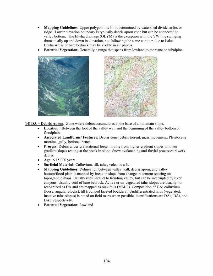
104
• Mapping Guidelines: Upper polygon line limit determined by watershed divide, arête, or
ridge. Lower elevation boundary is typically debris apron zone but can be connected to
valley bottom. The Elwha drainage (OLYM) is the exception with the VW line swinging
dramatically up and down in elevation, not following the same contour, due to Lake
Elwha.Areas of bare bedrock may be visible in air photos.
• Potential Vegetation: Generally a range that spans from lowland to montane or subalpine.
14) DA = Debris Apron. Zone where debris accumulates at the base of a mountain slope.
• Location: Between the foot of the valley wall and the beginning of the valley bottom or
floodplain.
• Associated Landforms/ Features: Debris cone, debris torrent, mass movement, Pleistocene
moraine, gully, bedrock bench.
• Process: Debris under gravitational force moving from higher gradient slopes to lower
gradient slopes resting at the break in slope. Snow avalanching and fluvial processes rework
debris.
• Age: < 15,000 years.
• Surficial Material: Colluvium, till, talus, volcanic ash.
• Mapping Guidelines: Delineation between valley wall, debris apron, and valley
bottom/flood plain is mapped by break in slope from change in contour spacing on
topographic maps. Usually runs parallel to trending valley, but can be interrupted by river
canyons. Usually void of bare bedrock. Active or un-vegetated talus slopes are usually not
recognized as DA and are mapped as rock falls (MM-F). Composition of DA; colluvium
(loose, angular blocks), till (rounded faceted boulders), Undifferentiated talus (vegetated,
inactive talus slopes) is noted on field maps when possible, identifications are DAc, DAt, and
DAu, respectively.
• Potential Vegetation: Lowland.
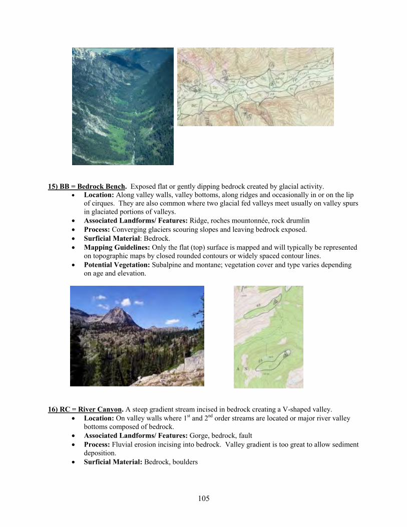
105
15) BB = Bedrock Bench. Exposed flat or gently dipping bedrock created by glacial activity.
• Location: Along valley walls, valley bottoms, along ridges and occasionally in or on the lip
of cirques. They are also common where two glacial fed valleys meet usually on valley spurs
in glaciated portions of valleys.
• Associated Landforms/ Features: Ridge, roches mountonnée, rock drumlin
• Process: Converging glaciers scouring slopes and leaving bedrock exposed.
• Surficial Material: Bedrock.
• Mapping Guidelines: Only the flat (top) surface is mapped and will typically be represented
on topographic maps by closed rounded contours or widely spaced contour lines.
• Potential Vegetation: Subalpine and montane; vegetation cover and type varies depending
on age and elevation.
16) RC = River Canyon. A steep gradient stream incised in bedrock creating a V-shaped valley.
• Location: On valley walls where 1st and 2
nd order streams are located or major river valley
bottoms composed of bedrock.
• Associated Landforms/ Features: Gorge, bedrock, fault
• Process: Fluvial erosion incising into bedrock. Valley gradient is too great to allow sediment
deposition.
• Surficial Material: Bedrock, boulders
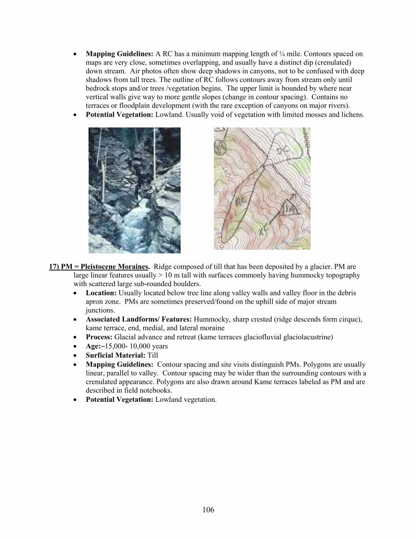
106
• Mapping Guidelines: A RC has a minimum mapping length of ¼ mile. Contours spaced on
maps are very close, sometimes overlapping, and usually have a distinct dip (crenulated)
down stream. Air photos often show deep shadows in canyons, not to be confused with deep
shadows from tall trees. The outline of RC follows contours away from stream only until
bedrock stops and/or trees /vegetation begins. The upper limit is bounded by where near
vertical walls give way to more gentle slopes (change in contour spacing). Contains no
terraces or floodplain development (with the rare exception of canyons on major rivers).
• Potential Vegetation: Lowland. Usually void of vegetation with limited mosses and lichens.
17) PM = Pleistocene Moraines. Ridge composed of till that has been deposited by a glacier. PM are
large linear features usually > 10 m tall with surfaces commonly having hummocky topography
with scattered large sub-rounded boulders.
• Location: Usually located below tree line along valley walls and valley floor in the debris
apron zone. PMs are sometimes preserved/found on the uphill side of major stream
junctions.
• Associated Landforms/ Features: Hummocky, sharp crested (ridge descends form cirque),
kame terrace, end, medial, and lateral moraine
• Process: Glacial advance and retreat (kame terraces glaciofluvial glaciolacustrine)
• Age:~15,000- 10,000 years
• Surficial Material: Till
• Mapping Guidelines: Contour spacing and site visits distinguish PMs. Polygons are usually
linear, parallel to valley. Contour spacing may be wider than the surrounding contours with a
crenulated appearance. Polygons are also drawn around Kame terraces labeled as PM and are
described in field notebooks.
• Potential Vegetation: Lowland vegetation.
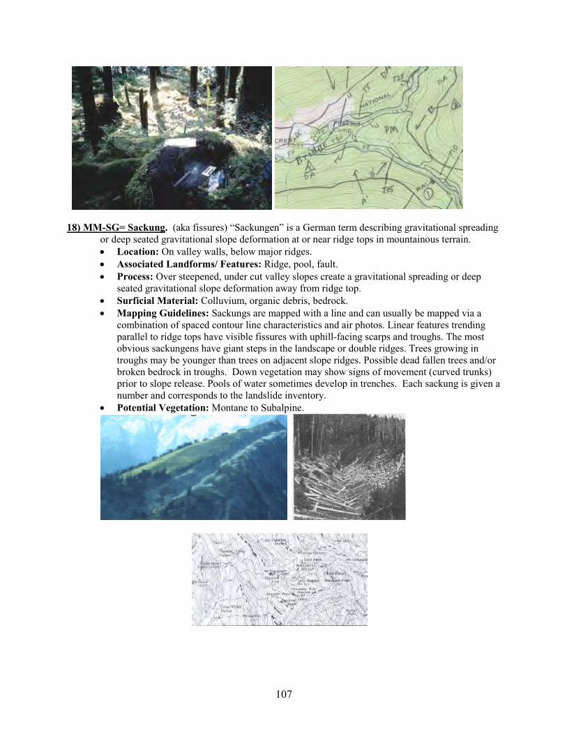
107
18) MM-SG= Sackung. (aka fissures) “Sackungen” is a German term describing gravitational spreading
or deep seated gravitational slope deformation at or near ridge tops in mountainous terrain.
• Location: On valley walls, below major ridges.
• Associated Landforms/ Features: Ridge, pool, fault.
• Process: Over steepened, under cut valley slopes create a gravitational spreading or deep
seated gravitational slope deformation away from ridge top.
• Surficial Material: Colluvium, organic debris, bedrock.
• Mapping Guidelines: Sackungs are mapped with a line and can usually be mapped via a
combination of spaced contour line characteristics and air photos. Linear features trending
parallel to ridge tops have visible fissures with uphill-facing scarps and troughs. The most
obvious sackungens have giant steps in the landscape or double ridges. Trees growing in
troughs may be younger than trees on adjacent slope ridges. Possible dead fallen trees and/or
broken bedrock in troughs. Down vegetation may show signs of movement (curved trunks)
prior to slope release. Pools of water sometimes develop in trenches. Each sackung is given a
number and corresponds to the landslide inventory.
• Potential Vegetation: Montane to Subalpine.
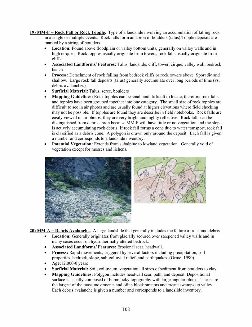
108
19) MM-F = Rock Fall or Rock Topple. Type of a landslide involving an accumulation of falling rock
in a single or multiple events. Rock falls form an apron of boulders (talus).Topple deposits are
marked by a string of boulders.
• Location: Found above floodplain or valley bottom units, generally on valley walls and in
high cirques. Rock topples usually originate from towers, rock falls usually originate from
cliffs.
• Associated Landforms/ Features: Talus, landslide, cliff, tower, cirque, valley wall, bedrock
bench
• Process: Detachment of rock falling from bedrock cliffs or rock towers above. Sporadic and
shallow. Large rock fall deposits (talus) generally accumulate over long periods of time (vs.
debris avalanches)
• Surficial Material: Talus, scree, boulders
• Mapping Guidelines: Rock topples can be small and difficult to locate, therefore rock falls
and topples have been grouped together into one category. The small size of rock topples are
difficult to see in air photos and are usually found at higher elevations where field checking
may not be possible. If topples are found they are describe in field notebooks. Rock falls are
easily viewed in air photos; they are very bright and highly reflective. Rock falls can be
distinguished from debris apron because MM-F will have little or no vegetation and the slope
is actively accumulating rock debris. If rock fall forms a cone due to water transport, rock fall
is classified as a debris cone. A polygon is drawn only around the deposit. Each fall is given
a number and corresponds to a landslide inventory.
• Potential Vegetation: Extends from subalpine to lowland vegetation. Generally void of
vegetation except for mosses and lichens.
20) MM-A = Debris Avalanche. A large landslide that generally includes the failure of rock and debris.
• Location: Generally originates from glacially scoured over steepened valley walls and in
many cases occur on hydrothermally altered bedrock.
• Associated Landforms/ Features: Erosional scar, headwall.
• Process: Rapid movements, triggered by several factors including precipitation, soil
properties, bedrock, slope, sub-colluvial relief, and earthquakes. (Orme, 1990).
• Age:12,000-0 years
• Surficial Material: Soil, colluvium, vegetation all sizes of sediment from boulders to clay.
• Mapping Guidelines: Polygon includes headwall scar, path, and deposit. Depositional
surface is usually composed of hummocky topography with large angular blocks. These are
the largest of the mass movements and often block streams and create swamps up valley.
Each debris avalanche is given a number and corresponds to a landslide inventory.
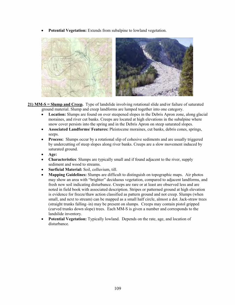
109
• Potential Vegetation: Extends from subalpine to lowland vegetation.
21) MM-S = Slump and Creep. Type of landslide involving rotational slide and/or failure of saturated
ground material. Slump and creep landforms are lumped together into one category.
• Location: Slumps are found on over steepened slopes in the Debris Apron zone, along glacial
moraines, and river cut banks. Creeps are located at high elevations in the subalpine where
snow cover persists into the spring and in the Debris Apron on steep saturated slopes.
• Associated Landforms/ Features: Pleistocene moraines, cut banks, debris cones, springs,
seeps.
• Process: Slumps occur by a rotational slip of cohesive sediments and are usually triggered
by undercutting of steep slopes along river banks. Creeps are a slow movement induced by
saturated ground.
• Age:
• Characteristics: Slumps are typically small and if found adjacent to the river, supply
sediment and wood to streams.
• Surficial Material: Soil, colluvium, till.
• Mapping Guidelines: Slumps are difficult to distinguish on topographic maps. Air photos may show an area with “brighter” deciduous vegetation, compared to adjacent landforms, and
fresh new soil indicating disturbance. Creeps are rare or at least are observed less and are
noted in field book with associated description. Stripes or patterned ground at high elevation
is evidence for freeze/thaw action classified as pattern ground and not creep. Slumps (when
small, and next to stream) can be mapped as a small half circle, almost a dot. Jack-straw trees
(straight trunks falling–in) may be present on slumps. Creeps may contain pistol gripped
(curved trunks down slope) trees. Each MM-S is given a number and corresponds to the
landslide inventory.
• Potential Vegetation: Typically lowland. Depends on the rate, age, and location of
disturbance.

110
22) MM-DT = Debris Torrent. Channelized debris flow.
• Location: Mapped only within the deposit of a debris cone and often found at the base of
river canyons, along fault zones, and hanging valleys.
• Associated Landforms/ Features: Levee, channel, river canyon, boulders.
• Process: Rapid and shallow. Rapid and/or sudden stream flow entrains debris stored in
stream channel while moving down slope. Debris is deposited onto gentler slopes below.
• Surficial Material: Colluvium (boulders, cobble, gravel), organic debris.
• Mapping Guidelines: The debris source should be examined but is not mapped. DT do not
extend above or below DC boundary. May contain the active stream. Levees are usually
present on either side of the channel and may have a lobe of debris at the toe. Each DT is
given a number and corresponds to the landslide inventory.
• Potential Vegetation: Lowland. Usually void of vegetation.
23) PD = Perched Delta. A relict delta formed under past Lake Elwha hrodrolic conditions.
• Location: High up within the debris apron zone or on the valley wall on larger tributary
streams. Thus far, found only within the Elwha Drainage.
• Associated Landforms/ Features: Terrace, large and broad
• Process: A gentle fan shaped deposit accumulating at the mouth of a stream where it met
relatively still water in a lake. Active fan abandoned when Lake Elwha drained
• Age: <15,000 years.
• Surficial Material: Alluvium, sand, silt, clay
• Mapping Guidelines: Recognizable on topographic maps as large broad area. Polygon is
drawn around entire feature with separation of terraces further broken out. Terrace levels are
checked in the field and are recorded in altitude. Usually, initial height is taken from lower

111
most contour of feature (refer to field books for specifics), each step in terrace is than
measured against first recorded height. Contours are usually shaped in a down trending lobe
from near apex near stream to old lake surface.
• Potential Vegetation: Lowland, more specifically lodgepole pine
24) PDC = Perched Debris Cone. A relict debris cone. Debris that was once deposited in a conical
shape with a surface slope greater than 10 degrees (perpendicular to contours). Under more recent
hydrolic conditions current stream dissects old debris cone leaving PDC as inactive.
• Location: High up within the debris apron zone or on the valley wall on a small stream
tributary. Thus far, found only within the Elwha Drainage.
• Associated Landforms/ Features: Debris torrent (at the mouth of 1st and 2
nd order tributaries
at the cone apex), scree slopes (at higher elevation zones) that exhibit a conical shape (AKA
alluvial cone, talus cone), avalanche chute, avalanche track, levee, SAIL, seeps, perched
debris cone terrace
• Process: Dissection occurring from major change in hydrolic structure on trunk river. Debris
transported by small streams or snow avalanches from valley walls and deposited at the break
in slope when a different hydrolic system was inplace (Lake Elwha). Debris was an
accumulation of many episodes where the stream channel or avalanche path changed course
back and forth creating a conical fan shape. The cone
• Age: <15,000 years.
• Surficial Material: Colluvium from bedrock upslope, till, scree, mass movement deposits
including boulders.
• Mapping Guidelines: Surface is covered with boulders and levees and can often contain
rock fall initiated from above. The toe of PDC can be truncated. Polygon is drawn around the
conical, fan-shaped contour lines on topographic maps or from field observations with aid of
altimeter. Polygon may be broken in two lobes with the current stream as the divider.
• Potential Vegetation: Lowland
25) PDCT = Perched Debris Cone Terrace. A flat area running parallel to the valley.
• Location: High up within the debris apron zone or on the valley wall on at the base of a
perched debris cone. Thus far, found only within the Elwha Drainage.
• Associated Landforms/ Features: Debris torrent (at the mouth of 1st and 2
nd order tributaries
at the cone apex), avalanche chute, avalanche track, levee, SAIL, seeps, perched debris cone.
• Process: The deposit of a debris cone under different hydrolic conditions than present where
past Lake Elwha surface level fluctuated.
• Age: <15,000 years.
• Surficial Material: Alluvium
• Mapping Guidelines: Features are found usually only by field investigation or with the aid
of LIDAR. Polygon is drawn around the flat area. Terraces can be steeped on a single
perched debris cone. (Talk about how to measure height if we want height) PDT are mapped
on 3rd order or larger streams. The polygon is focused on the tributary valley vs. an elongated
terraces running the Elwha valley.
• Potential Vegetation: Lowland
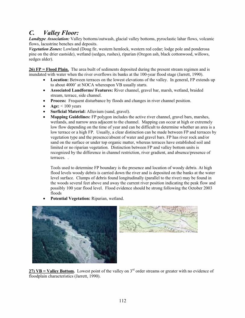
112
C. Valley Floor: Landtype Association: Valley bottoms/outwash, glacial valley bottoms, pyroclastic lahar flows, volcanic
flows, lacustrine benches and deposits.
Vegetation Zones: Lowland (Doug fir, western hemlock, western red cedar; lodge pole and ponderosa
pine on the drier eastside), wetland (sedges, rushes), riparian (Oregon ash, black cottonwood, willows,
sedges alder). 26) FP = Flood Plain. The area built of sediments deposited during the present stream regimen and is
inundated with water when the river overflows its banks at the 100-year flood stage (Jarrett, 1990).
• Location: Between terraces on the lowest elevations of the valley. In general, FP extends up
to about 4000’ at NOCA whereupon VB usually starts.
• Associated Landforms/ Features: River channel, gravel bar, marsh, wetland, braided
stream, terrace, side channel.
• Process: Frequent disturbance by floods and changes in river channel position.
• Age: < 100 years
• Surficial Material: Alluvium (sand, gravel).
• Mapping Guidelines: FP polygon includes the active river channel, gravel bars, marshes,
wetlands, and narrow area adjacent to the channel. Mapping can occur at high or extremely
low flow depending on the time of year and can be difficult to determine whether an area is a
low terrace or a high FP. Usually, a clear distinction can be made between FP and terraces by
vegetation type and the presence/absent of water and gravel bars. FP has river rock and/or
sand on the surface or under top organic matter, whereas terraces have established soil and
limited or no riparian vegetation. Distinction between FP and valley bottom units is
recognized by the difference in channel restriction, river gradient, and absence/presence of
terraces. .
Tools used to determine FP boundary is the presence and location of woody debris. At high
flood levels woody debris is carried down the river and is deposited on the banks at the water
level surface. Clumps of debris found longitudinally (parallel to the river) may be found in
the woods several feet above and away the current river position indicating the peak flow and
possibly 100 year flood level. Flood evidence should be strong following the October 2003
floods
• Potential Vegetation: Riparian, wetland.
27) VB = Valley Bottom. Lowest point of the valley on 3rd order streams or greater with no evidence of
floodplain characteristics (Jarrett, 1990).

113
• Location: Within NOCA, valley bottom usually begins around 4000ft elevation with flood
plain below (see floodplain). Within MORA, valley bottom is mapped at elevations above
the furthest extent of Little Ice Age glaciers within the watershed. VB does not generally
extend into high elevation cirque basins.
• Associated Landforms/ Features: Active channel, cutbank, debris cone, debris apron, SAIL.
• Process: Areas at head of valleys where sediment supply generally exceed streams ability to
remove. Thus minimal evidence for cut and fill (terraces). Occurs generally above rain on
snow zone (i.e. lower peak flows, ~4,000’)
• Age: <100 years old
• Surficial Material: Alluvium (sand, gravel)
• Mapping Guidelines: Polygon is drawn to include the active river and adjacent, gently
sloping boundary. Polygon is typically less than several hundred feet wide. Merges at lower
elevation with flood plain and at the upper elevation with valley wall, cirque, and debris
apron. Area contains no terraces or other ways to identify it as flood plain. May have a
slightly higher stream gradient than flood plain. VB can be broken by areas of lower gradient
where sediment is stored and terraces form.
• Potential Vegetation: Usually montane and subalpine with small areas of riparian.
28) T = Terrace. A relatively flat surface that grades gently downstream and represents the dissected
remnants of a previous flood plain.
• Location: On the valley floor between the active river/flood plain and debris apron. Within
NOCA, terraces generally have not been found at elevations above 4000ft.
• Associated Landforms/ Features: Old side channel, flood plain, escarpment on stream side.
• Process: Erosional or depositional feature. River incising into floodplain leaving behind an
older surface.
• Age: > 100 years old
• Surficial Material: Alluvium, sand and gravel below soil, glacial outwash.
• Mapping Guidelines: Terraces are represented by widely spaced contours adjacent to the
active river. Surface gently slopes down valley, verses debris apron, which slopes toward the
center of the valley. Remnants of abandoned side channels can cause terrace surface to be
slightly uneven. Steep sides are represented by hatched lines on field maps. Terraces at high
elevation are generally smaller. All terraces are field checked for height and composition.
Notes of composition, typically alluvium (younger), outwash (older), or lacustrine (clay)
deposits are recorded in field notebooks when possible. Within MORA terraces are
subdivided by the following guidelines; Terrace elevations are marked in feet above stream
channel (i.e. T-5 or T-12). (see floodplain for more distinction) Within NOCA, terraces can
further be described by age using the following guidelines; Terraces <5ft date to the
(FP
(VB
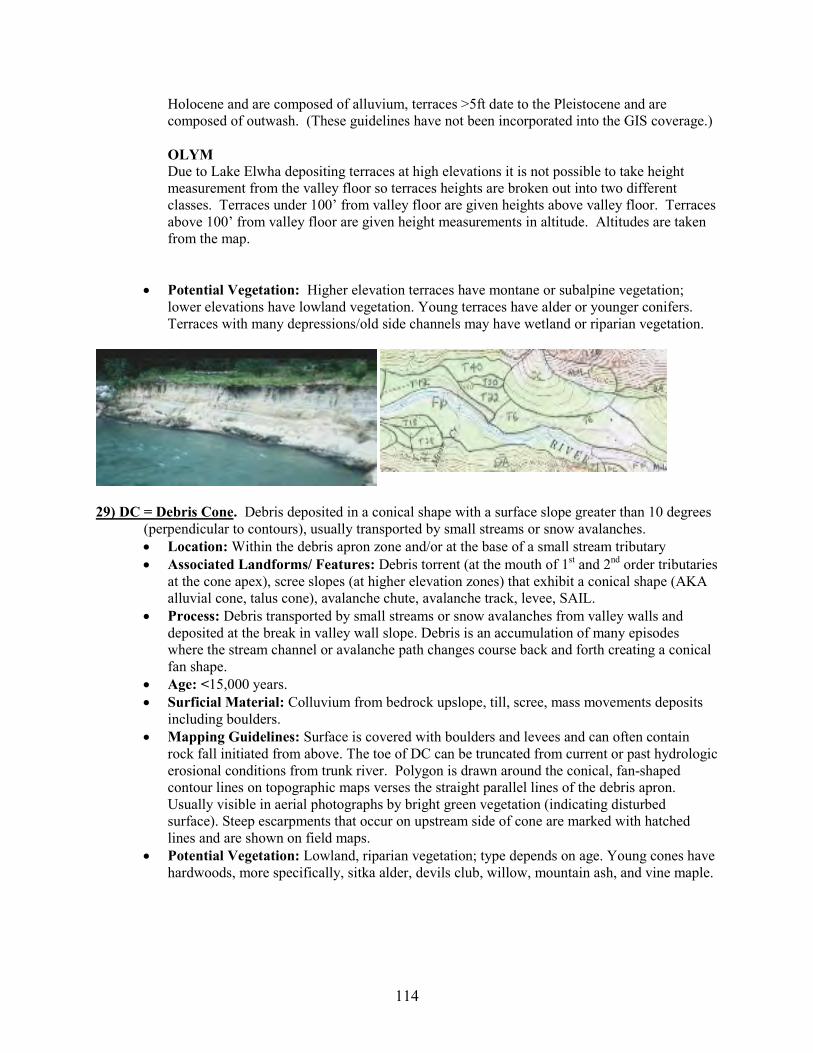
114
Holocene and are composed of alluvium, terraces >5ft date to the Pleistocene and are
composed of outwash. (These guidelines have not been incorporated into the GIS coverage.)
OLYM Due to Lake Elwha depositing terraces at high elevations it is not possible to take height
measurement from the valley floor so terraces heights are broken out into two different
classes. Terraces under 100’ from valley floor are given heights above valley floor. Terraces
above 100’ from valley floor are given height measurements in altitude. Altitudes are taken
from the map.
• Potential Vegetation: Higher elevation terraces have montane or subalpine vegetation;
lower elevations have lowland vegetation. Young terraces have alder or younger conifers.
Terraces with many depressions/old side channels may have wetland or riparian vegetation.
29) DC = Debris Cone. Debris deposited in a conical shape with a surface slope greater than 10 degrees
(perpendicular to contours), usually transported by small streams or snow avalanches.
• Location: Within the debris apron zone and/or at the base of a small stream tributary
• Associated Landforms/ Features: Debris torrent (at the mouth of 1st and 2
nd order tributaries
at the cone apex), scree slopes (at higher elevation zones) that exhibit a conical shape (AKA
alluvial cone, talus cone), avalanche chute, avalanche track, levee, SAIL.
• Process: Debris transported by small streams or snow avalanches from valley walls and
deposited at the break in valley wall slope. Debris is an accumulation of many episodes
where the stream channel or avalanche path changes course back and forth creating a conical
fan shape.
• Age: <15,000 years.
• Surficial Material: Colluvium from bedrock upslope, till, scree, mass movements deposits
including boulders.
• Mapping Guidelines: Surface is covered with boulders and levees and can often contain
rock fall initiated from above. The toe of DC can be truncated from current or past hydrologic
erosional conditions from trunk river. Polygon is drawn around the conical, fan-shaped
contour lines on topographic maps verses the straight parallel lines of the debris apron.
Usually visible in aerial photographs by bright green vegetation (indicating disturbed
surface). Steep escarpments that occur on upstream side of cone are marked with hatched
lines and are shown on field maps.
• Potential Vegetation: Lowland, riparian vegetation; type depends on age. Young cones have
hardwoods, more specifically, sitka alder, devils club, willow, mountain ash, and vine maple.
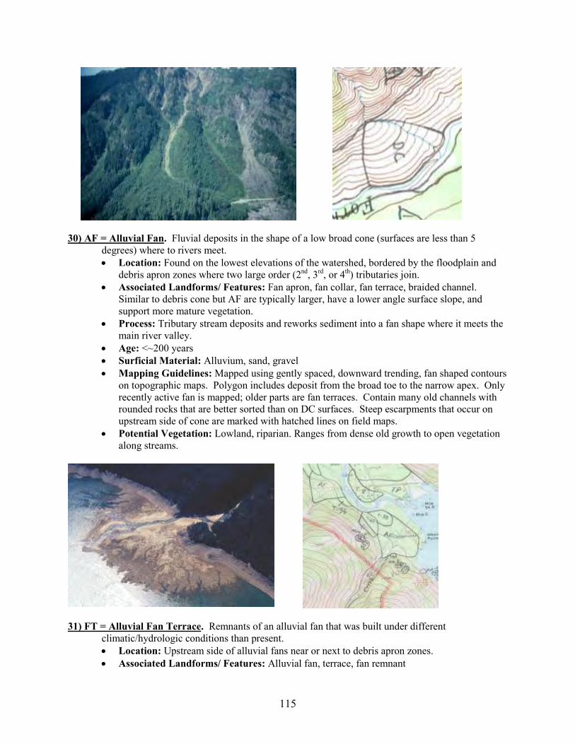
115
30) AF = Alluvial Fan. Fluvial deposits in the shape of a low broad cone (surfaces are less than 5
degrees) where to rivers meet.
• Location: Found on the lowest elevations of the watershed, bordered by the floodplain and
debris apron zones where two large order (2nd, 3
rd, or 4
th) tributaries join.
• Associated Landforms/ Features: Fan apron, fan collar, fan terrace, braided channel.
Similar to debris cone but AF are typically larger, have a lower angle surface slope, and
support more mature vegetation.
• Process: Tributary stream deposits and reworks sediment into a fan shape where it meets the
main river valley.
• Age: <~200 years
• Surficial Material: Alluvium, sand, gravel
• Mapping Guidelines: Mapped using gently spaced, downward trending, fan shaped contours
on topographic maps. Polygon includes deposit from the broad toe to the narrow apex. Only
recently active fan is mapped; older parts are fan terraces. Contain many old channels with
rounded rocks that are better sorted than on DC surfaces. Steep escarpments that occur on
upstream side of cone are marked with hatched lines on field maps.
• Potential Vegetation: Lowland, riparian. Ranges from dense old growth to open vegetation
along streams.
31) FT = Alluvial Fan Terrace. Remnants of an alluvial fan that was built under different
climatic/hydrologic conditions than present.
• Location: Upstream side of alluvial fans near or next to debris apron zones.
• Associated Landforms/ Features: Alluvial fan, terrace, fan remnant
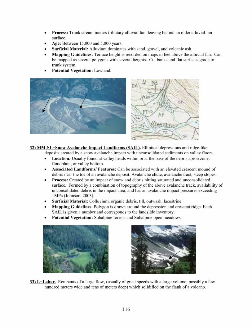
116
• Process: Trunk stream incises tributary alluvial fan, leaving behind an older alluvial fan
surface.
• Age: Between 15,000 and 5,000 years.
• Surficial Material: Alluvium dominates with sand, gravel, and volcanic ash.
• Mapping Guidelines: Terrace height is recorded on maps in feet above the alluvial fan. Can
be mapped as several polygons with several heights. Cut banks and flat surfaces grade to
trunk system.
• Potential Vegetation: Lowland.
32) MM-SL=Snow Avalanche Impact Landforms (SAIL). Elliptical depressions and ridge-like
deposits created by a snow avalanche impact with unconsolidated sediments on valley floors.
• Location: Usually found at valley heads within or at the base of the debris apron zone,
floodplain, or valley bottom.
• Associated Landforms/ Features: Can be associated with an elevated crescent mound of
debris near the toe of an avalanche deposit. Avalanche chute, avalanche tract, steep slopes.
• Process: Created by an impact of snow and debris hitting saturated and unconsolidated
surface. Formed by a combination of topography of the above avalanche track, availability of
unconsolidated debris in the impact area, and has an avalanche impact pressures exceeding
1MPa (Johnson, 2003).
• Surficial Material: Colluvium, organic debris, till, outwash, lacustrine.
• Mapping Guidelines: Polygon is drawn around the depression and crescent ridge. Each
SAIL is given a number and corresponds to the landslide inventory.
• Potential Vegetation: Subalpine forests and Subalpine open meadows.
33) L=Lahar. Remnants of a large flow, (usually of great speeds with a large volume; possibly a few
hundred meters wide and tens of meters deep) which solidified on the flank of a volcano.
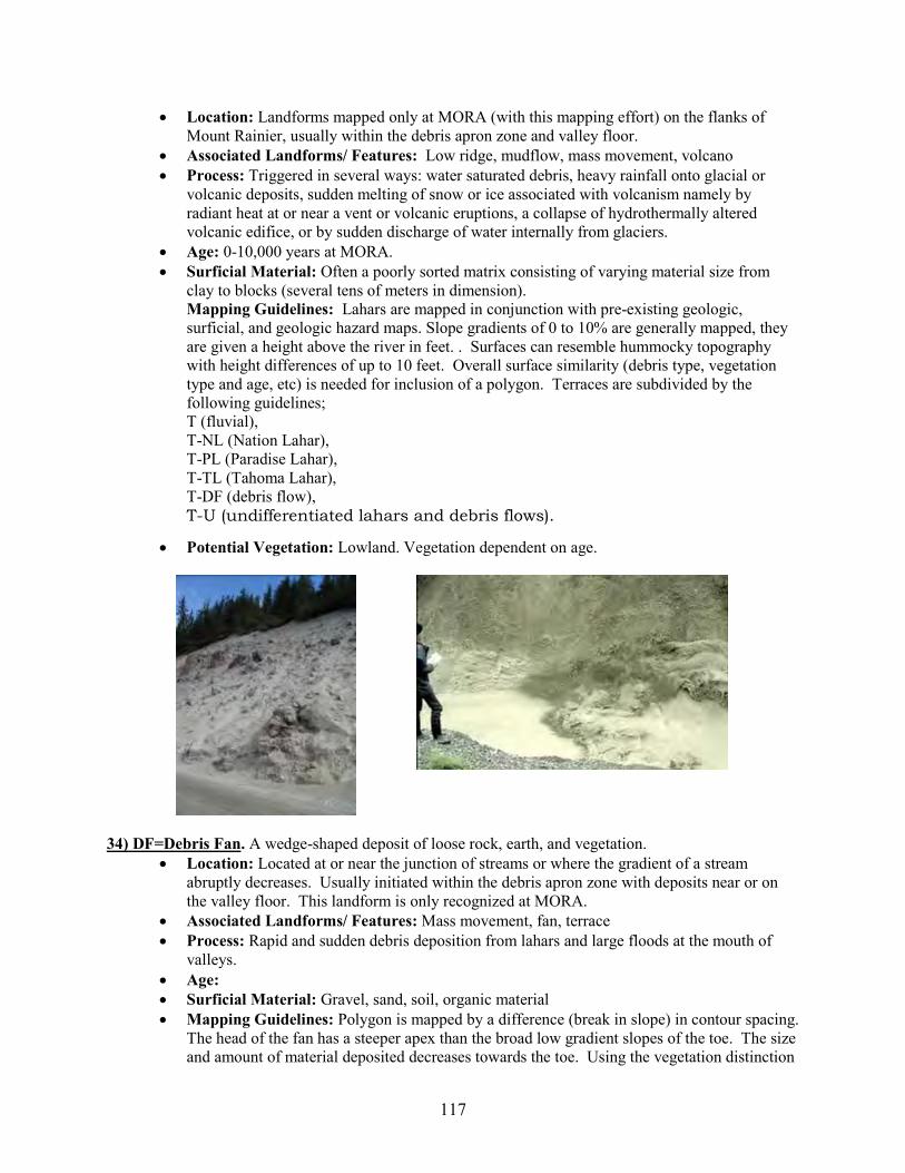
117
• Location: Landforms mapped only at MORA (with this mapping effort) on the flanks of
Mount Rainier, usually within the debris apron zone and valley floor.
• Associated Landforms/ Features: Low ridge, mudflow, mass movement, volcano
• Process: Triggered in several ways: water saturated debris, heavy rainfall onto glacial or
volcanic deposits, sudden melting of snow or ice associated with volcanism namely by
radiant heat at or near a vent or volcanic eruptions, a collapse of hydrothermally altered
volcanic edifice, or by sudden discharge of water internally from glaciers.
• Age: 0-10,000 years at MORA.
• Surficial Material: Often a poorly sorted matrix consisting of varying material size from
clay to blocks (several tens of meters in dimension).
Mapping Guidelines: Lahars are mapped in conjunction with pre-existing geologic,
surficial, and geologic hazard maps. Slope gradients of 0 to 10% are generally mapped, they
are given a height above the river in feet. . Surfaces can resemble hummocky topography
with height differences of up to 10 feet. Overall surface similarity (debris type, vegetation
type and age, etc) is needed for inclusion of a polygon. Terraces are subdivided by the
following guidelines;
T (fluvial),
T-NL (Nation Lahar),
T-PL (Paradise Lahar),
T-TL (Tahoma Lahar),
T-DF (debris flow),
T-U (undifferentiated lahars and debris flows).
• Potential Vegetation: Lowland. Vegetation dependent on age.
34) DF=Debris Fan. A wedge-shaped deposit of loose rock, earth, and vegetation.
• Location: Located at or near the junction of streams or where the gradient of a stream
abruptly decreases. Usually initiated within the debris apron zone with deposits near or on
the valley floor. This landform is only recognized at MORA.
• Associated Landforms/ Features: Mass movement, fan, terrace
• Process: Rapid and sudden debris deposition from lahars and large floods at the mouth of
valleys.
• Age:
• Surficial Material: Gravel, sand, soil, organic material
• Mapping Guidelines: Polygon is mapped by a difference (break in slope) in contour spacing.
The head of the fan has a steeper apex than the broad low gradient slopes of the toe. The size
and amount of material deposited decreases towards the toe. Using the vegetation distinction
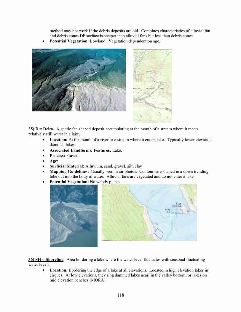
118
method may not work if the debris deposits are old. Combines characteristics of alluvial fan
and debris cones DF surface is steeper than alluvial fans but less than debris cones
• Potential Vegetation: Lowland. Vegetation dependent on age.
35) D = Delta. A gentle fan shaped deposit accumulating at the mouth of a stream where it meets
relatively still water in a lake.
• Location: At the mouth of a river or a stream where it enters lake. Typically lower elevation
dammed lakes.
• Associated Landforms/ Features: Lake.
• Process: Fluvial.
• Age:
• Surficial Material: Alluvium, sand, gravel, silt, clay
• Mapping Guidelines: Usually seen in air photos. Contours are shaped in a down trending
lobe out into the body of water. Alluvial fans are vegetated and do not enter a lake.
• Potential Vegetation: No woody plants.
36) SH = Shoreline. Area bordering a lake where the water level fluctuates with seasonal fluctuating
water levels.
• Location: Bordering the edge of a lake at all elevations. Located in high elevation lakes in
cirques. At low elevations, they ring dammed lakes near/ in the valley bottom; or lakes on
mid elevation benches (MORA).
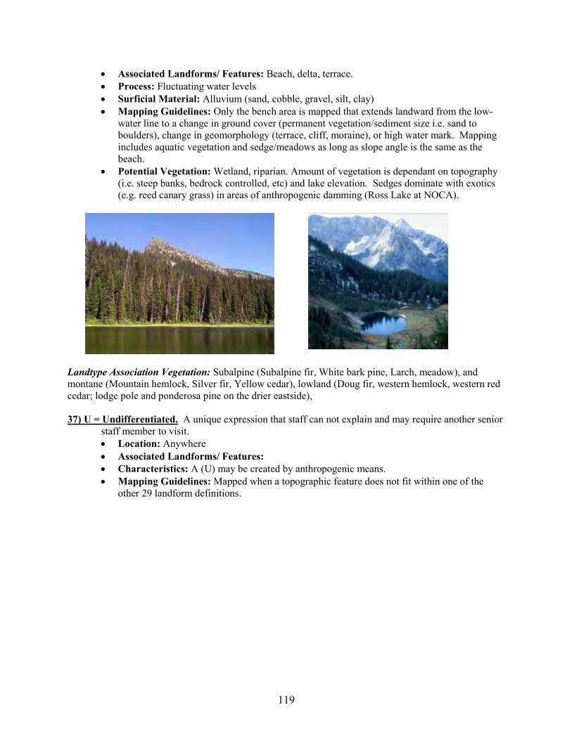
119
• Associated Landforms/ Features: Beach, delta, terrace.
• Process: Fluctuating water levels
• Surficial Material: Alluvium (sand, cobble, gravel, silt, clay)
• Mapping Guidelines: Only the bench area is mapped that extends landward from the low-
water line to a change in ground cover (permanent vegetation/sediment size i.e. sand to
boulders), change in geomorphology (terrace, cliff, moraine), or high water mark. Mapping
includes aquatic vegetation and sedge/meadows as long as slope angle is the same as the
beach.
• Potential Vegetation: Wetland, riparian. Amount of vegetation is dependant on topography
(i.e. steep banks, bedrock controlled, etc) and lake elevation. Sedges dominate with exotics
(e.g. reed canary grass) in areas of anthropogenic damming (Ross Lake at NOCA).
Landtype Association Vegetation: Subalpine (Subalpine fir, White bark pine, Larch, meadow), and
montane (Mountain hemlock, Silver fir, Yellow cedar), lowland (Doug fir, western hemlock, western red
cedar; lodge pole and ponderosa pine on the drier eastside),
37) U = Undifferentiated. A unique expression that staff can not explain and may require another senior
staff member to visit.
• Location: Anywhere
• Associated Landforms/ Features:
• Characteristics: A (U) may be created by anthropogenic means.
• Mapping Guidelines: Mapped when a topographic feature does not fit within one of the
other 29 landform definitions.
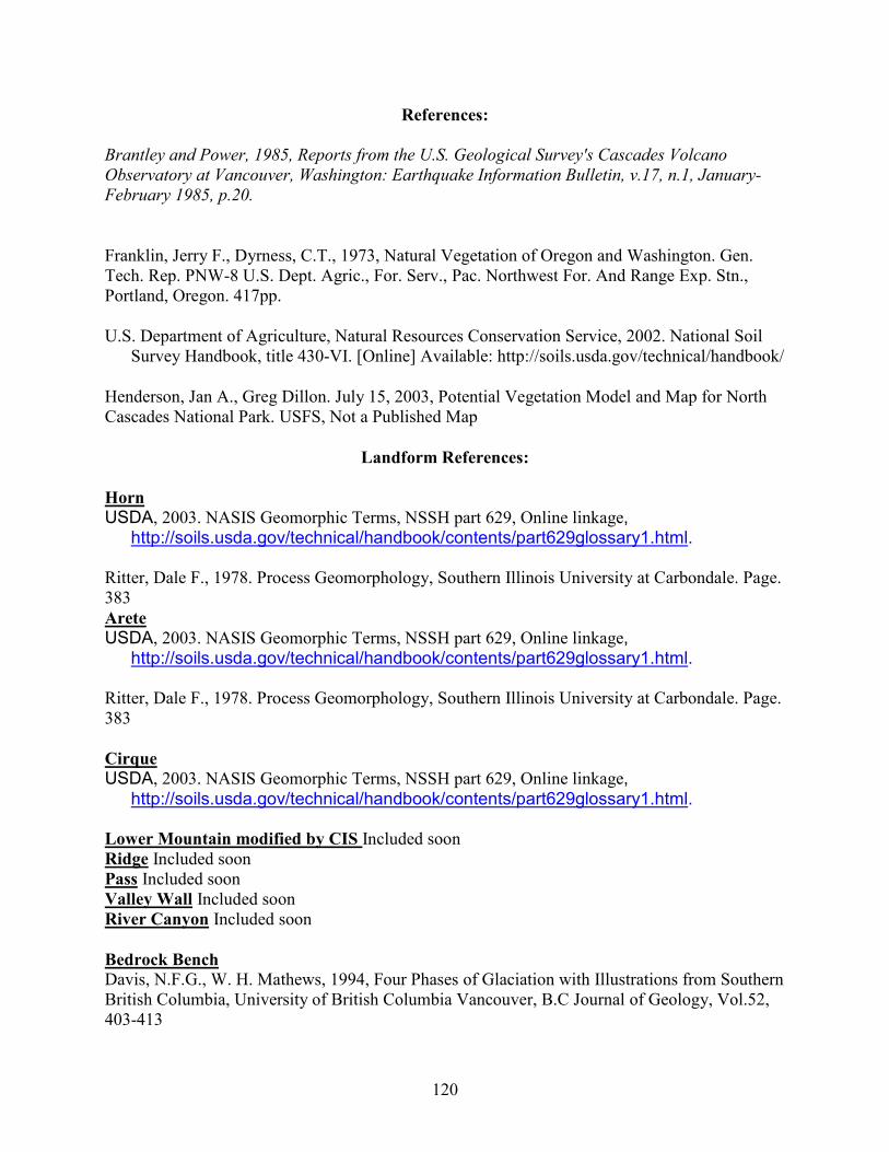
120
References:
Brantley and Power, 1985, Reports from the U.S. Geological Survey's Cascades Volcano
Observatory at Vancouver, Washington: Earthquake Information Bulletin, v.17, n.1, January-
February 1985, p.20.
Franklin, Jerry F., Dyrness, C.T., 1973, Natural Vegetation of Oregon and Washington. Gen.
Tech. Rep. PNW-8 U.S. Dept. Agric., For. Serv., Pac. Northwest For. And Range Exp. Stn.,
Portland, Oregon. 417pp.
U.S. Department of Agriculture, Natural Resources Conservation Service, 2002. National Soil
Survey Handbook, title 430-VI. [Online] Available: http://soils.usda.gov/technical/handbook/
Henderson, Jan A., Greg Dillon. July 15, 2003, Potential Vegetation Model and Map for North
Cascades National Park. USFS, Not a Published Map
Landform References:
Horn
USDA, 2003. NASIS Geomorphic Terms, NSSH part 629, Online linkage, http://soils.usda.gov/technical/handbook/contents/part629glossary1.html.
Ritter, Dale F., 1978. Process Geomorphology, Southern Illinois University at Carbondale. Page.
383
Arete
USDA, 2003. NASIS Geomorphic Terms, NSSH part 629, Online linkage, http://soils.usda.gov/technical/handbook/contents/part629glossary1.html.
Ritter, Dale F., 1978. Process Geomorphology, Southern Illinois University at Carbondale. Page.
383
Cirque
USDA, 2003. NASIS Geomorphic Terms, NSSH part 629, Online linkage, http://soils.usda.gov/technical/handbook/contents/part629glossary1.html.
Lower Mountain modified by CIS Included soon
Ridge Included soon
Pass Included soon
Valley Wall Included soon
River Canyon Included soon
Bedrock Bench Davis, N.F.G., W. H. Mathews, 1994, Four Phases of Glaciation with Illustrations from Southern
British Columbia, University of British Columbia Vancouver, B.C Journal of Geology, Vol.52,
403-413
121
Cleaver Volcanic Cone (Volcanic Valley Side-A conical hill of lava and/or pyroclastics that is built up
around a volcanic vent. The sloping to very steep surfaces between the valley floor and summits
of adjacent uplands. Well-defined, steep valley sides have been termed valley walls.)
USDA, 2003. NASIS Geomorphic Terms, NSSH part 629, Online linkage, http://soils.usda.gov/technical/handbook/contents/part629glossary1.html.
Park The American Geologic Institute. 1984. Dictionary of Geological Terms. p.571
(A term used in the Rocky Mountain region of Colorad and Wyoming for a wide, grassy open
valley lying at a high altitude and walled in by wooded mountains.)
Rock Fall and Topple Cruden, D.M., D.J. Varnes. 1996. Landslide Types and Processes. Landslides Investigation and
Mitigation, Transportation Research Board Special Report 247, Chapter 3.
Debris Avalanches (large size, rapid) Orme, Antony, R. 1990. Recurrence of Debris Production under Coniferous Forest, Cascades
Foothills, John Wiley & Sons Ltd., Vegetation and Erosion, Northwest United States
Department of Geography, University of California,
Haskins, Donald M. et.al., USFS, 1998. A geomorphic Classification System. Version 1.4
Slump and Creep Pringle, Patrick, T., The Nisqually Landslide of September 1990, Washington Geologic
Newsletter, Vol. 18, No.4
Debris Torrents Orme, Antony, R. 1990. Recurrence of Debris Production under Coniferous Forest, Cascades
Foothills, John Wiley & Sons Ltd., Vegetation and Erosion, Northwest United States
Department of Geography, University of California
Eisbacher, G.H. and J.J. Clague, 1984. Slope Failure and Mass Movements, Destructive Mass
Movements in High Mountains: Hazards and Management, Geological Survey of Canada
Paper 84-16,
Suckung McCalpin, J.P., 2001, Bibliography of Papers on Sackungen, Gravitational Spreading, Deep-
Seated Slope Failures, Mass Rock Creep, and Stress State in Steep Slopes. Geo-Haz
Consulting, Inc
McCalpin, James, P., 2001, Holocene Displacement history of ridge top depressions (Sackungen
in the San Gabriel Mountains, Southern CA, GEO-HAZ Consulting, Inc.
122
Schwab,j.w., Kirk, W. 2002, Sackungen on a forested slope, Kitnayawa River, British Columbia
Ministry of Forests, Prince Rupert Forest Region. Extention Notes, Issue 47
Rowland, Tabor. July 1971, Origin of Ridge-Top Depression by Large-Scale Creep in the
Olympic Mountains, Washington, Geological Society of America Bulletin, v. 82, p.1811-
1822
Varnes, D.J., et al, 2000. Measurement of ridge-spreading movements (Sackungen) at Bald Eagle
Mountain, Lake County, CO, II: continuation of the 1975-1989 measurements using a Global
Positioning System in 1997 and 1999. USGS open file report 00-205, on-line edition
Varnes, D.J., D.H. Radbruch-Hall, and W.Z. Savage. 1989. Topographic and Structural
Conditions in Areas of Gravitationsl Spreading of Ridges in the Western United States. U.S.
Geological Survey Professional Paper 1496, 28 pp.
SAIL (Snow Avalanche Impact Landform Johnson, A.L., Smith, D.J., 2003. What are Snow avalanche impact landforms?, University of
Victoria, BC, On the Edge, 2003
Debris Apron Included soon
Debris Cone Eisbacher, G.H. and J.J. Clague, 1984. Slope Failure and Mass Movements, Destructive Mass
Movements in High Mountains: Hazards and Management, Geological Survey of Canada
Paper 84-16.
Alluvial Fan Orme, Antony, R., 1989. Alluvial Fans. Physical Geography, 1989, 10, 2, pp. 131-146
USDA, 2003. NASIS Geomorphic Terms, NSSH part 629, On line linkage, http://soils.usda.gov/technical/handbook/contents/part629glossary1.html.
Debris Fan Ministry of Crown Lands Province of British Columbia, 1997. Terrain Classification System for
British Columbia. MOE Manual 10 (Version 2) (p.13) Fisheries Branch, Ministry of
Environment
Colorado geological survey (CGS), June 30, 2003 Special Publication 12. Debris Fan
Lahar Dwight R. Crandell, 1971, Postglacial Lahars From Mount Rainier Volcano, Washington USGS
Professional Paper 677
Tilling, Topinka, and Swanson, 1990, Eruptions of Mount St. Helens: Past, Present, and Future

123
USDA, 2003. NASIS Geomorphic Terms, NSSH part 629, Online linkage, http://soils.usda.gov/technical/handbook/contents/part629glossary1.html.
Miller, 1989, Potential Hazards from Future Volcanic Eruptions in California: USGS Bulletin
1847
Floodplain Jarrett, Robert D., 1990.Hydrologic and Hydraulic Research in Mountain Rivers. Water
Resources Bulletin, American Water Resource Association. Vol. 26, NO.3
USDA, 2003. NASIS Geomorphic Terms, NSSH part 629, Online linkage,
http://soils.usda.gov/technical/handbook/contents/part629glossary1.html.
Valley Bottom Jarrett, Robert D., 1990.Hydrologic and Hydraulic Research in Mountain Rivers. Water
Resources Bulletin, American Water Resource Association. Vol. 26, NO.3
Terraces
USDA, 2003. NASIS Geomorphic Terms, NSSH part 629, On line linkage, http://soils.usda.gov/technical/handbook/contents/part629glossary1.html.
Fan Terrace Included soon
Pleistocene Moraine The American Geologic Institute. 1984. Dictionary of Geological Terms. p.571
(PleistoceneAn epoch of the Quaternary period, after the Pliocene ot the Tertiary and before the
Holocene..It began two to three million years ago…..Syn: ice age; glacial epoch. )
Little Ice Age and other Holocene Moraines Included soon
Patterned Ground
USDA, 2003. NASIS Geomorphic Terms, NSSH part 629, Online linkage, http://soils.usda.gov/technical/handbook/contents/part629glossary1.html.
Ritter, Dale F., 1978. Process Geomorphology, Southern Illinois University at Carbondale. Page.
447
Volcanic Crater The American Geologic Institute. 1984. Dictionary of Geological Terms. p.571
(Crater- A basin-like, rimmed structure at the top or on the flanks of a volcanic cone: it is a
result formed by explosion or collapse.)
124
APPENDIX B
NATIONAL PARK SERVICE LANDFORM MAPS
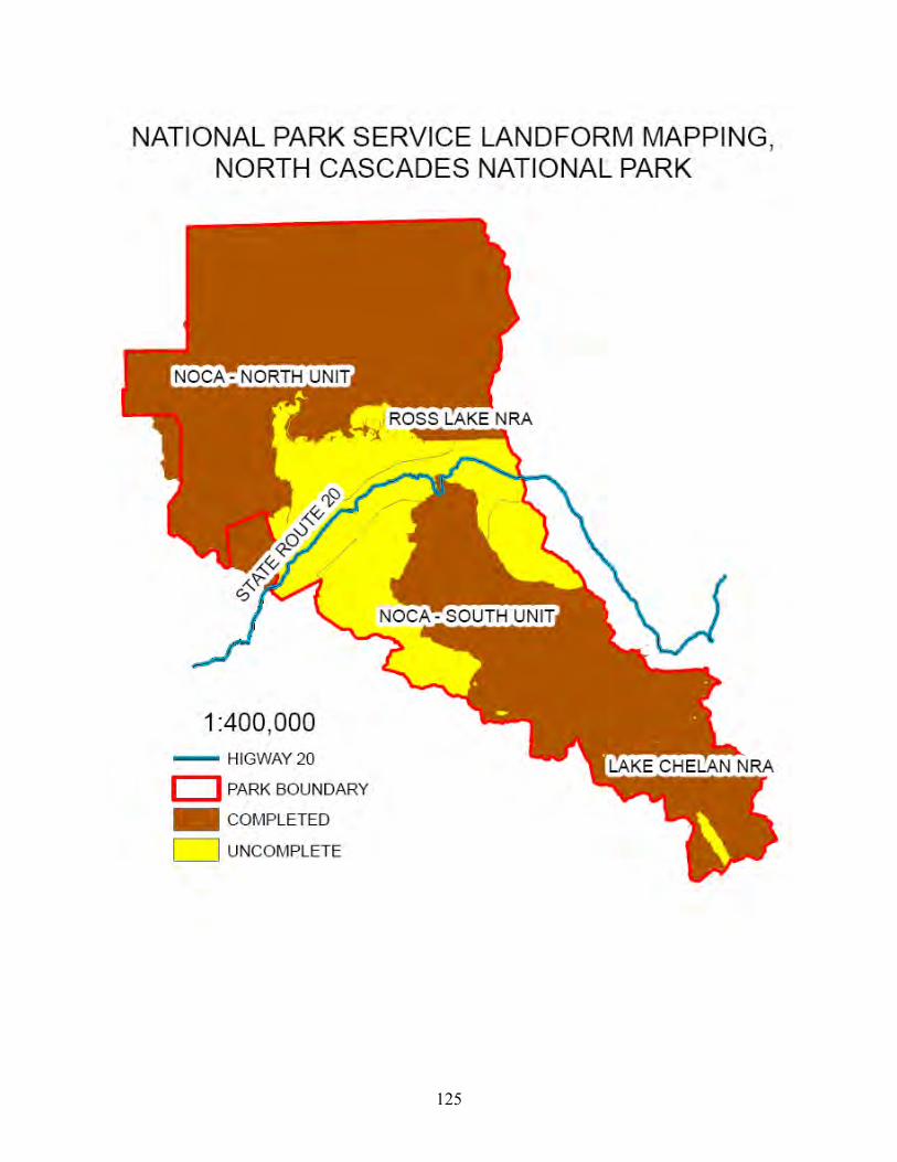
125
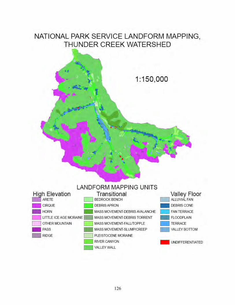
126

APPENDIX C
NORTH CASCADES PLANT LIST
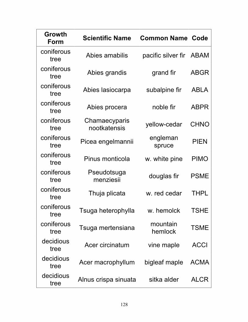
128
Growth Form
Scientific Name Common Name Code
coniferous tree
Abies amabilis pacific silver fir ABAM
coniferous tree
Abies grandis grand fir ABGR
coniferous tree
Abies lasiocarpa subalpine fir ABLA
coniferous tree
Abies procera noble fir ABPR
coniferous tree
Chamaecyparis nootkatensis
yellow-cedar CHNO
coniferous tree
Picea engelmannii engleman spruce
PIEN
coniferous tree
Pinus monticola w. white pine PIMO
coniferous tree
Pseudotsuga menziesii
douglas fir PSME
coniferous tree
Thuja plicata w. red cedar THPL
coniferous tree
Tsuga heterophylla w. hemolck TSHE
coniferous tree
Tsuga mertensiana mountain hemlock
TSME
decidious tree
Acer circinatum vine maple ACCI
decidious tree
Acer macrophyllum bigleaf maple ACMA
decidious tree
Alnus crispa sinuata sitka alder ALCR
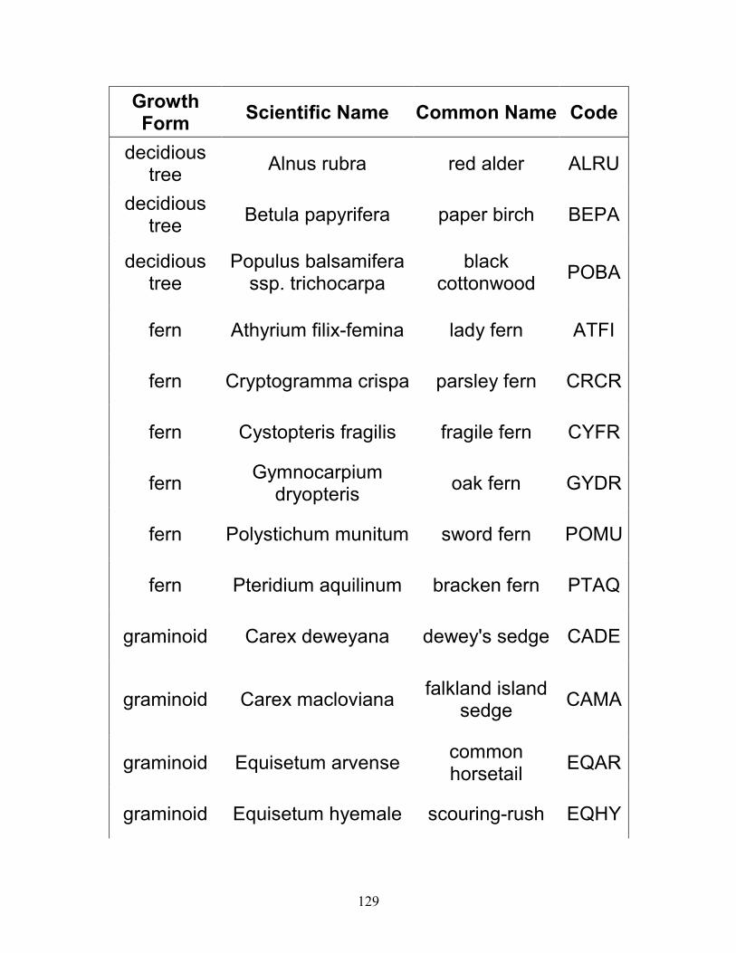
129
Growth Form
Scientific Name Common Name Code
decidious tree
Alnus rubra red alder ALRU
decidious tree
Betula papyrifera paper birch BEPA
decidious tree
Populus balsamifera ssp. trichocarpa
black cottonwood
POBA
fern Athyrium filix-femina lady fern ATFI
fern Cryptogramma crispa parsley fern CRCR
fern Cystopteris fragilis fragile fern CYFR
fern Gymnocarpium
dryopteris oak fern GYDR
fern Polystichum munitum sword fern POMU
fern Pteridium aquilinum bracken fern PTAQ
graminoid Carex deweyana dewey's sedge CADE
graminoid Carex macloviana falkland island
sedge CAMA
graminoid Equisetum arvense common horsetail
EQAR
graminoid Equisetum hyemale scouring-rush EQHY

130
Growth Form
Scientific Name Common Name
Code
mosses Hylocomium splendens
step moss HYSP
mosses Lycopodium annotinum
stiff clubmoss LYAN
shrub Amelanchier alnifolia saskatoon AMAL
shrub Cornus stolonifera red osier dogwood
COST
shrub Gaultheria shallon salal GASH
shrub Holodiscus discolor oceanspray HODI
shrub Mahonia nervosa dull oregon
grape MANE
shrub Menziesia ferruginea fool's
huckleberry MEFE
shrub Oplopanax horridus devil's club OPHO
shrub Pachistima myrsinites pachistima PAMY
shrub Rubes divaricatum wild gooseberry RIDI
shrub Ribes lacustre black
gooseberry RILA
shrub Ribes sanguineum red flowering
current RISA
shrub Rosa gymnocarpa baldhip rose ROGY

131
Growth Form
Scientific Name Common Name
Code
shrub Rubus leucodermis black rasberry RULE
shrub Rubus parviflorus thimbleberry RUPA
shrub Rubus pedatus 5-leaved bramble
RUPE
shrub Rubus spectabilis salmonberry RUSP
shrub Rubus ursinus trailing
blackberry RUUR
shrub Sambucus racemosa
ssp. pubens elderberry (red) SARA
shrub Salix sitchensis sitka willow SASI
shrub Sorbus sitchensis mt. ash SOSI
shrub Symphoricacarpos
albus snowberry SYAL
shrub Urtica dioca stinging nettle URDI
shrub Vaccinium ovalifolium oval-leaved blueberry
VAOV
shrub Vaccinium
membranaceum black
huckleberry VAME
shrub Vaccinium parvifolium red huckleberry VAPA
wildflower Achillea millefolium yarrow ACMI
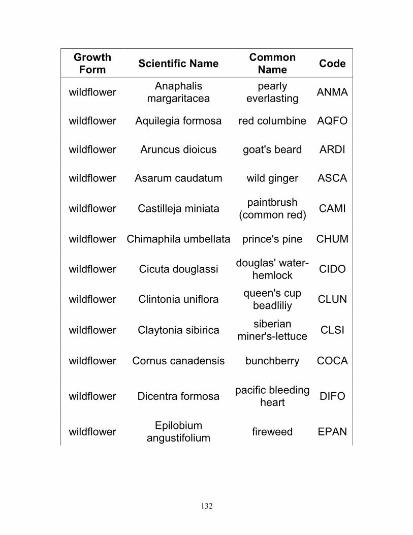
132
Growth Form
Scientific Name Common Name
Code
wildflower Anaphalis
margaritacea pearly
everlasting ANMA
wildflower Aquilegia formosa red columbine AQFO
wildflower Aruncus dioicus goat's beard ARDI
wildflower Asarum caudatum wild ginger ASCA
wildflower Castilleja miniata paintbrush
(common red) CAMI
wildflower Chimaphila umbellata prince's pine CHUM
wildflower Cicuta douglassi douglas' water-
hemlock CIDO
wildflower Clintonia uniflora queen's cup beadliliy
CLUN
wildflower Claytonia sibirica siberian
miner's-lettuce CLSI
wildflower Cornus canadensis bunchberry COCA
wildflower Dicentra formosa pacific bleeding
heart DIFO
wildflower Epilobium
angustifolium fireweed EPAN
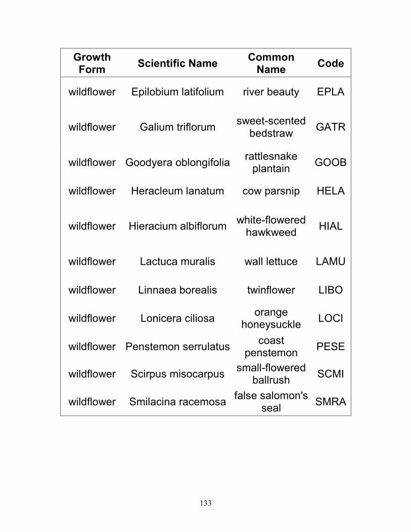
133
Growth Form
Scientific Name Common Name
Code
wildflower Epilobium latifolium river beauty EPLA
wildflower Galium triflorum sweet-scented
bedstraw GATR
wildflower Goodyera oblongifolia rattlesnake plantain
GOOB
wildflower Heracleum lanatum cow parsnip HELA
wildflower Hieracium albiflorum white-flowered hawkweed
HIAL
wildflower Lactuca muralis wall lettuce LAMU
wildflower Linnaea borealis twinflower LIBO
wildflower Lonicera ciliosa orange
honeysuckle LOCI
wildflower Penstemon serrulatus coast
penstemon PESE
wildflower Scirpus misocarpus small-flowered
ballrush SCMI
wildflower Smilacina racemosa false salomon's
seal SMRA
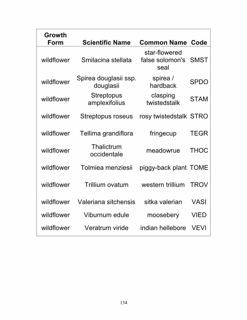
134
Growth Form Scientific Name Common Name Code
wildflower Smilacina stellata star-flowered
false solomon's seal
SMST
wildflower Spirea douglasii ssp.
douglasii spirea / hardback
SPDO
wildflower Streptopus amplexifolius
clasping twistedstalk
STAM
wildflower Streptopus roseus rosy twistedstalk STRO
wildflower Tellima grandiflora fringecup TEGR
wildflower Thalictrum occidentale
meadowrue THOC
wildflower Tolmiea menziesii piggy-back plant TOME
wildflower Trillium ovatum western trillium TROV
wildflower Valeriana sitchensis sitka valerian VASI
wildflower Viburnum edule moosebery VIED
wildflower Veratrum viride indian hellebore VEVI