digital image processing lectures 5 & 6

Digital Image ProcessingLectures 5 & 6

Mahmood (Mo) Azimi, Professor

Colorado State University

Fort Collins, Co 80523

email : [email protected]

Each time you have to click on this icon

wherever it appears to load the next sound file

To advance click enter or page down to go back use page up

http://webctce.colostate.edu/CSUshared/realmedia_files/ee/ee513_azimi/lecture5_6/lecture5_6.ram

1. Parseval’s Theorem and Inner Product Preservation

Another important property of FT is that the inner product of

two functions is equal to the inner product of their FT’s.∫ ∫ ∞

−∞x(v, u)y∗(u, v)dudv

=1

4π2

∫ ∫ ∞

−∞X(ω1, ω2)Y ∗(ω1, ω2)dω1dω2

where ∗ stands for complex conjugate operation. When x = y

we obtain the well-known Parseval energy conservation formula

i.e.∫ ∫ ∞

−∞|x(u, v)|2dudv =

14π2

∫ ∫ ∞

−∞|X(ω1, ω2)|2dω1dω2

i.e. the total energy in the function is the same as in its FT.

2. Frequency Response and Eigenfunctions of 2-D LSI Systems

An eigen-function of a system is defined as an input function

To advance click enter or page down to go back use page up 1

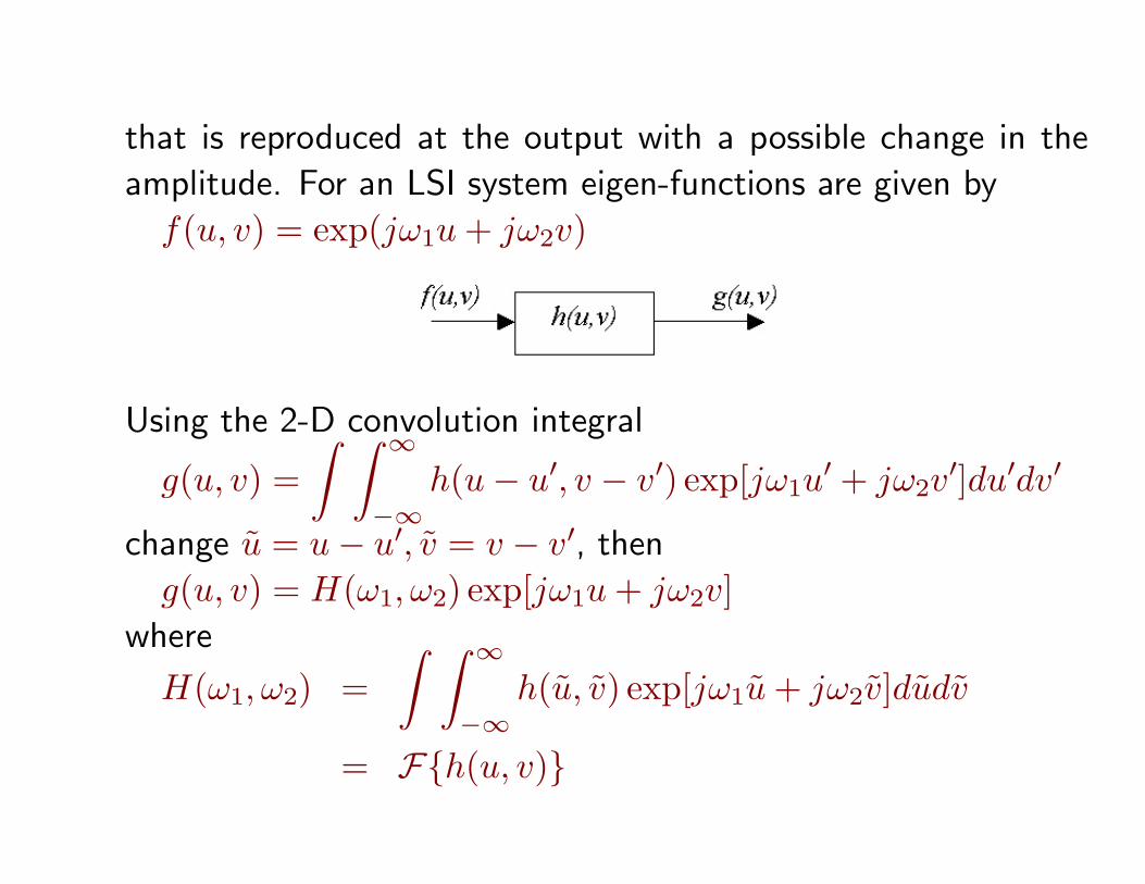
that is reproduced at the output with a possible change in the

amplitude. For an LSI system eigen-functions are given by

f(u, v) = exp(jω1u + jω2v)

Using the 2-D convolution integral

g(u, v) =∫ ∫ ∞

−∞h(u− u′, v − v′) exp[jω1u

′ + jω2v′]du′dv′

change u = u− u′, v = v − v′, then

g(u, v) = H(ω1, ω2) exp[jω1u + jω2v]where

H(ω1, ω2) =∫ ∫ ∞

−∞h(u, v) exp[jω1u + jω2v]dudv

= Fh(u, v)


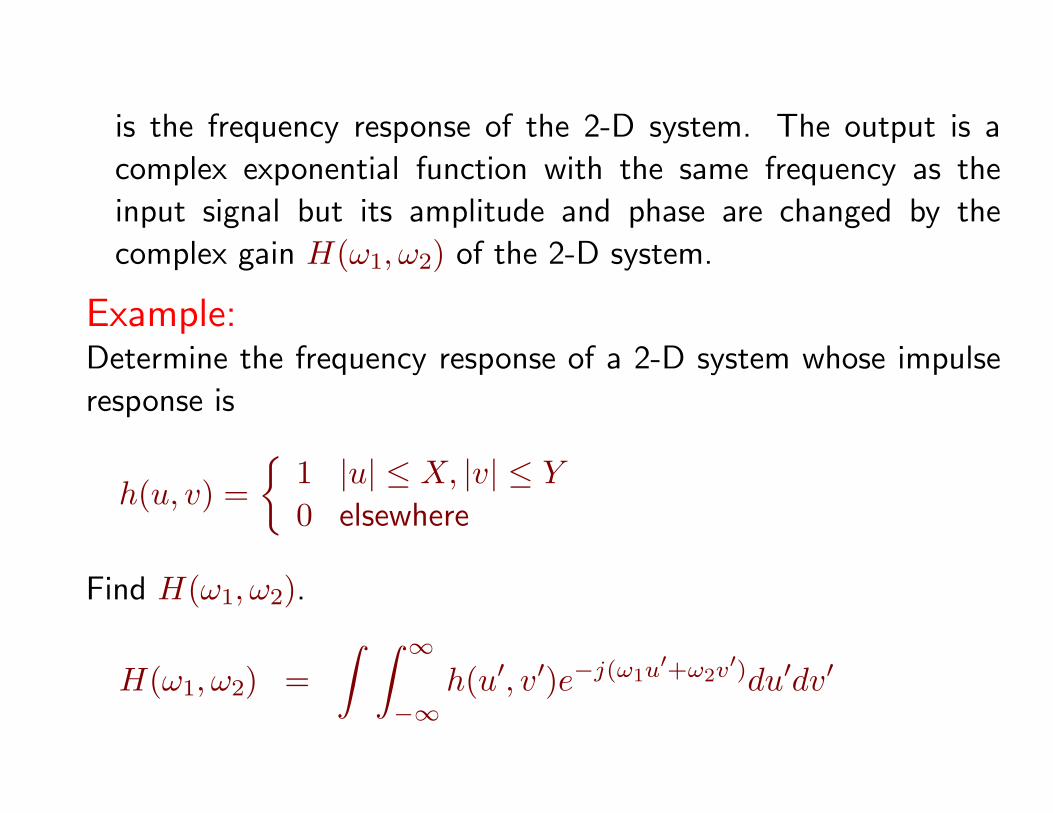
is the frequency response of the 2-D system. The output is a

complex exponential function with the same frequency as the

input signal but its amplitude and phase are changed by the

complex gain H(ω1, ω2) of the 2-D system.

Example:Determine the frequency response of a 2-D system whose impulse

response is

h(u, v) =

1 |u| ≤ X, |v| ≤ Y

0 elsewhere

Find H(ω1, ω2).

H(ω1, ω2) =∫ ∫ ∞

−∞h(u′, v′)e−j(ω1u′+ω2v′)du′dv′


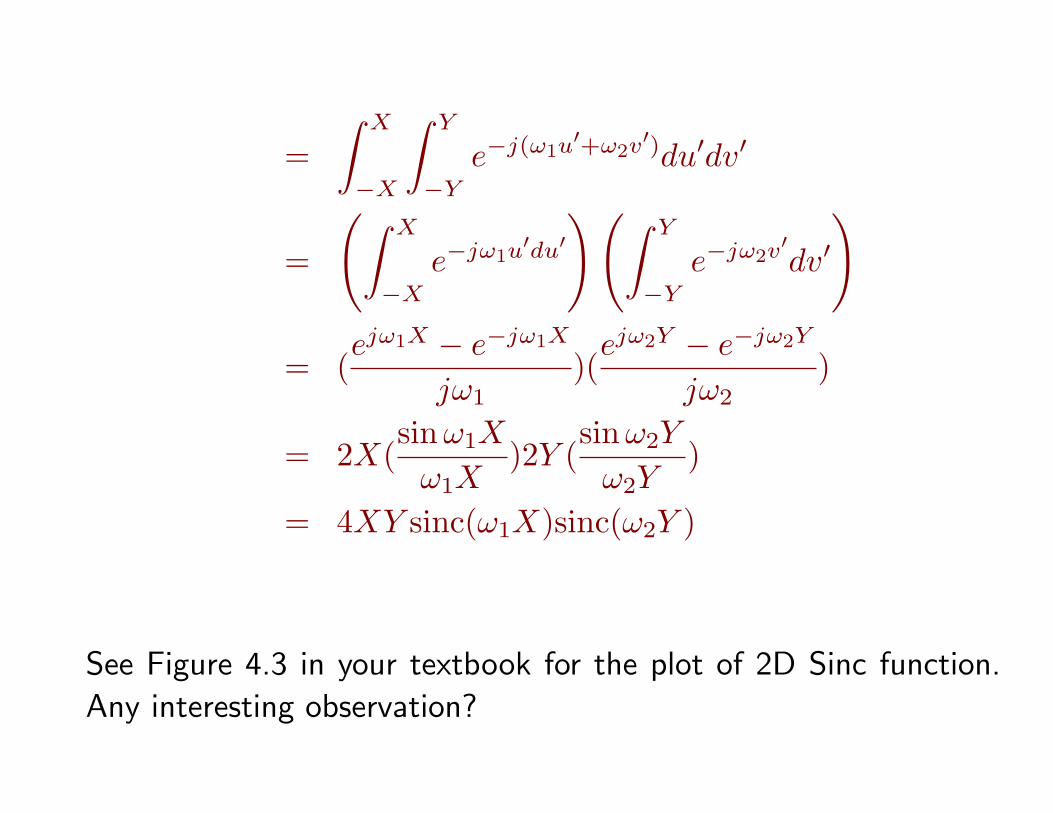
=∫ X

−X

∫ Y

−Y

e−j(ω1u′+ω2v′)du′dv′

=

(∫ X

−X

e−jω1u′du′

)(∫ Y

−Y

e−jω2v′dv′

)

= (ejω1X − e−jω1X

jω1)(

ejω2Y − e−jω2Y

jω2)

= 2X(sinω1X

ω1X)2Y (

sinω2Y

ω2Y)

= 4XY sinc(ω1X)sinc(ω2Y )

See Figure 4.3 in your textbook for the plot of 2D Sinc function.

Any interesting observation?


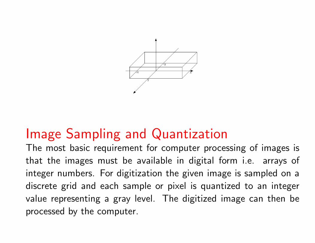
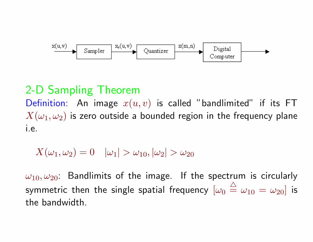
Image Sampling and QuantizationThe most basic requirement for computer processing of images is

that the images must be available in digital form i.e. arrays of

integer numbers. For digitization the given image is sampled on a

discrete grid and each sample or pixel is quantized to an integer

value representing a gray level. The digitized image can then be

processed by the computer.


2-D Sampling TheoremDefinition: An image x(u, v) is called ”bandlimited” if its FT

X(ω1, ω2) is zero outside a bounded region in the frequency plane

i.e.

X(ω1, ω2) = 0 |ω1| > ω10, |ω2| > ω20

ω10, ω20: Bandlimits of the image. If the spectrum is circularly

symmetric then the single spatial frequency [ω04= ω10 = ω20] is

the bandwidth.


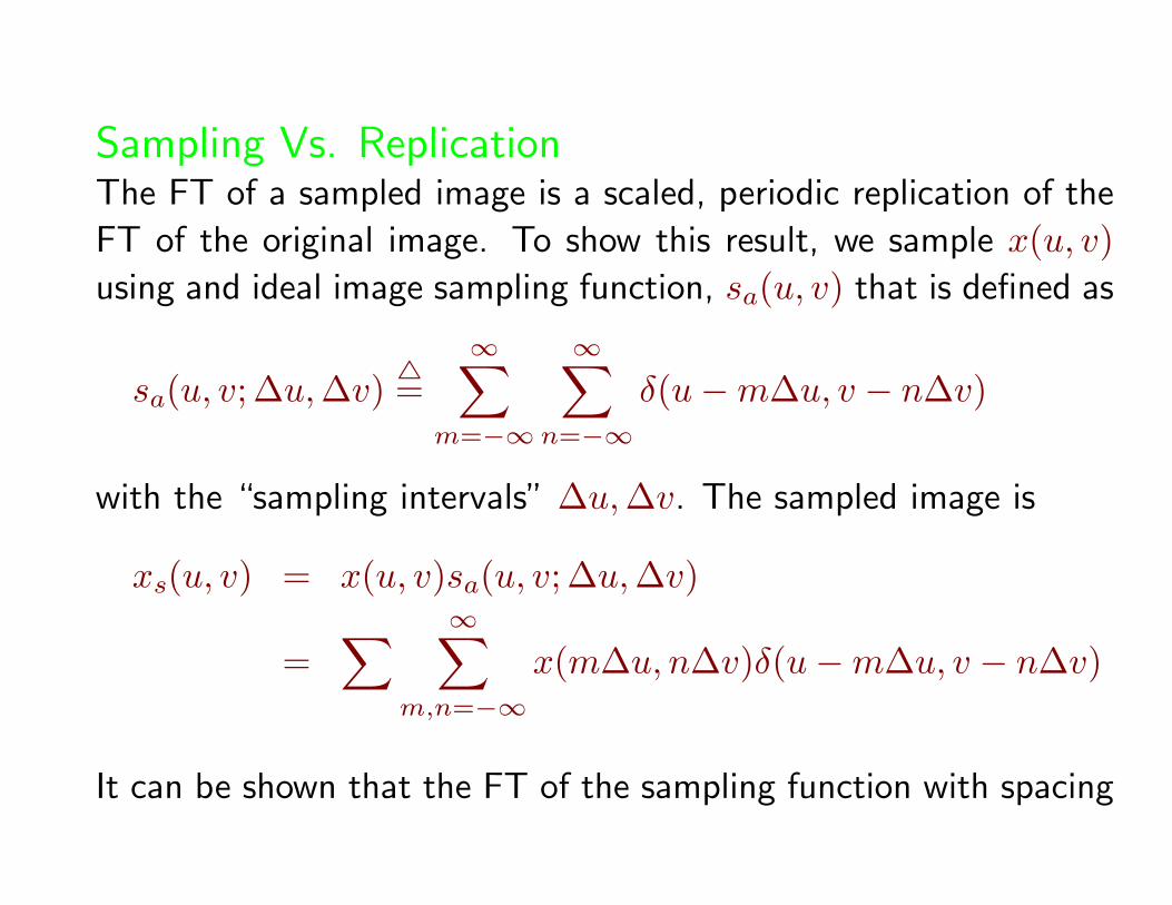
Sampling Vs. ReplicationThe FT of a sampled image is a scaled, periodic replication of the

FT of the original image. To show this result, we sample x(u, v)using and ideal image sampling function, sa(u, v) that is defined as

sa(u, v;∆u, ∆v)4=

∞∑m=−∞

∞∑n=−∞

δ(u−m∆u, v − n∆v)

with the “sampling intervals” ∆u, ∆v. The sampled image is

xs(u, v) = x(u, v)sa(u, v;∆u, ∆v)

=∑ ∞∑

m,n=−∞x(m∆u, n∆v)δ(u−m∆u, v − n∆v)

It can be shown that the FT of the sampling function with spacing


∆u, ∆v is another sampling function with spacing 2π∆u, 2π

∆v. Then,

using the convolution in frequency domain we get

Xs(ω1, ω2) =1

∆u∆v

∑ ∞∑k,l=−∞

X(ω1 −2πk

∆u, ω2 −

2πl

∆v)

Let us define discrete frequency variables (i.e. in discrete

domain) Ω1∆=ω1∆u,Ω2

∆=ω2∆v, then we get 2-D Discrete Space Fourier

Transform (DSFT),

Xs(Ω1,Ω2) =1

∆u∆v

∑ ∞∑k,l=−∞

X(Ω1 − 2πk

∆u,Ω2 − 2πl

∆v)

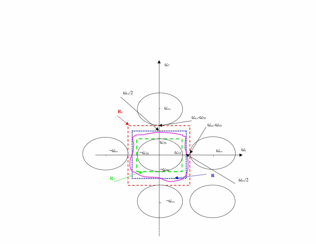
This result shows sampling in the spatial domain causes periodicity

in the frequency domain (See Figure).


ω20

−ω10 ω10

−ω20

ω2

ω1

ωvs

−ωvs

−ωus ωus

ωus-ω10

ωvs-ω20

R1

R R2

ωvs/2

ωus/2


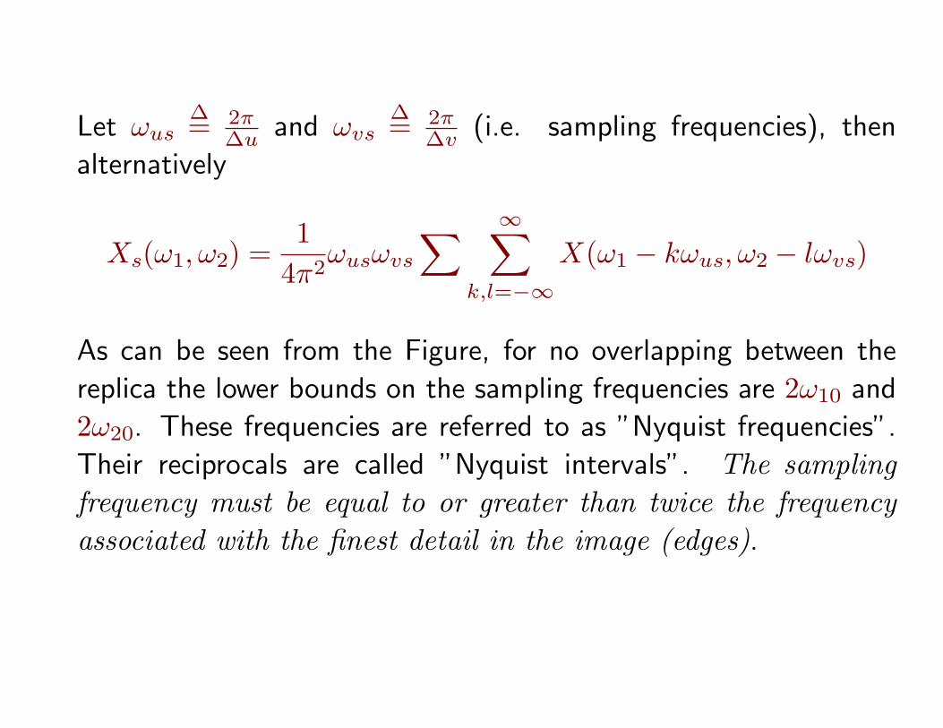
Let ωus∆= 2π

∆u and ωvs∆= 2π

∆v (i.e. sampling frequencies), then

alternatively

Xs(ω1, ω2) =1

4π2ωusωvs

∑ ∞∑k,l=−∞

X(ω1 − kωus, ω2 − lωvs)

As can be seen from the Figure, for no overlapping between the

replica the lower bounds on the sampling frequencies are 2ω10 and

2ω20. These frequencies are referred to as ”Nyquist frequencies”.

Their reciprocals are called ”Nyquist intervals”. The samplingfrequency must be equal to or greater than twice the frequencyassociated with the finest detail in the image (edges).


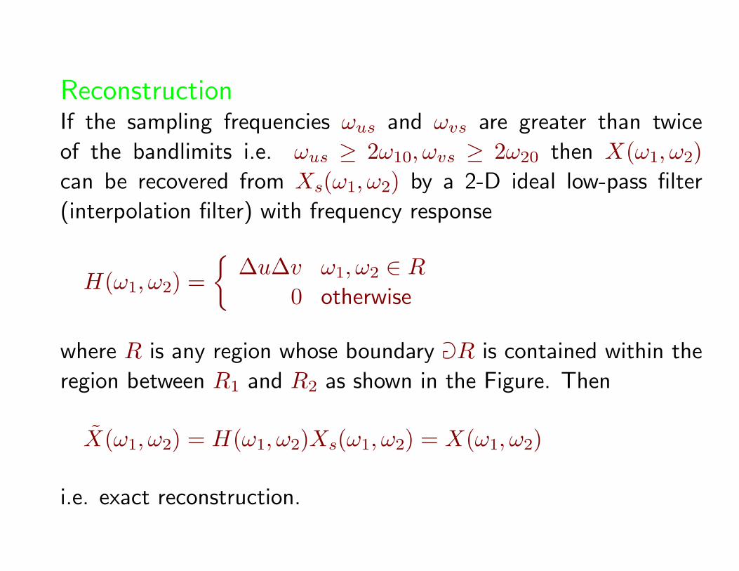
ReconstructionIf the sampling frequencies ωus and ωvs are greater than twice

of the bandlimits i.e. ωus ≥ 2ω10, ωvs ≥ 2ω20 then X(ω1, ω2)can be recovered from Xs(ω1, ω2) by a 2-D ideal low-pass filter

(interpolation filter) with frequency response

H(ω1, ω2) =

∆u∆v ω1, ω2 ∈ R

0 otherwise

where R is any region whose boundary aR is contained within the

region between R1 and R2 as shown in the Figure. Then

X(ω1, ω2) = H(ω1, ω2)Xs(ω1, ω2) = X(ω1, ω2)

i.e. exact reconstruction.


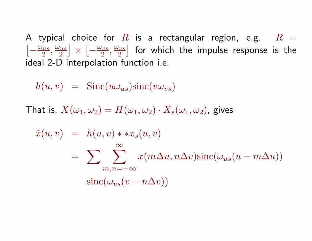
A typical choice for R is a rectangular region, e.g. R =[−ωus

2 , ωus2

]×[−ωvs

2 , ωvs2

]for which the impulse response is the

ideal 2-D interpolation function i.e.

h(u, v) = Sinc(uωus)sinc(vωvs)

That is, X(ω1, ω2) = H(ω1, ω2) ·Xs(ω1, ω2), gives

x(u, v) = h(u, v) ∗ ∗xs(u, v)

=∑ ∞∑

m,n=−∞x(m∆u, n∆v)sinc(ωus(u−m∆u))

sinc(ωvs(v − n∆v))


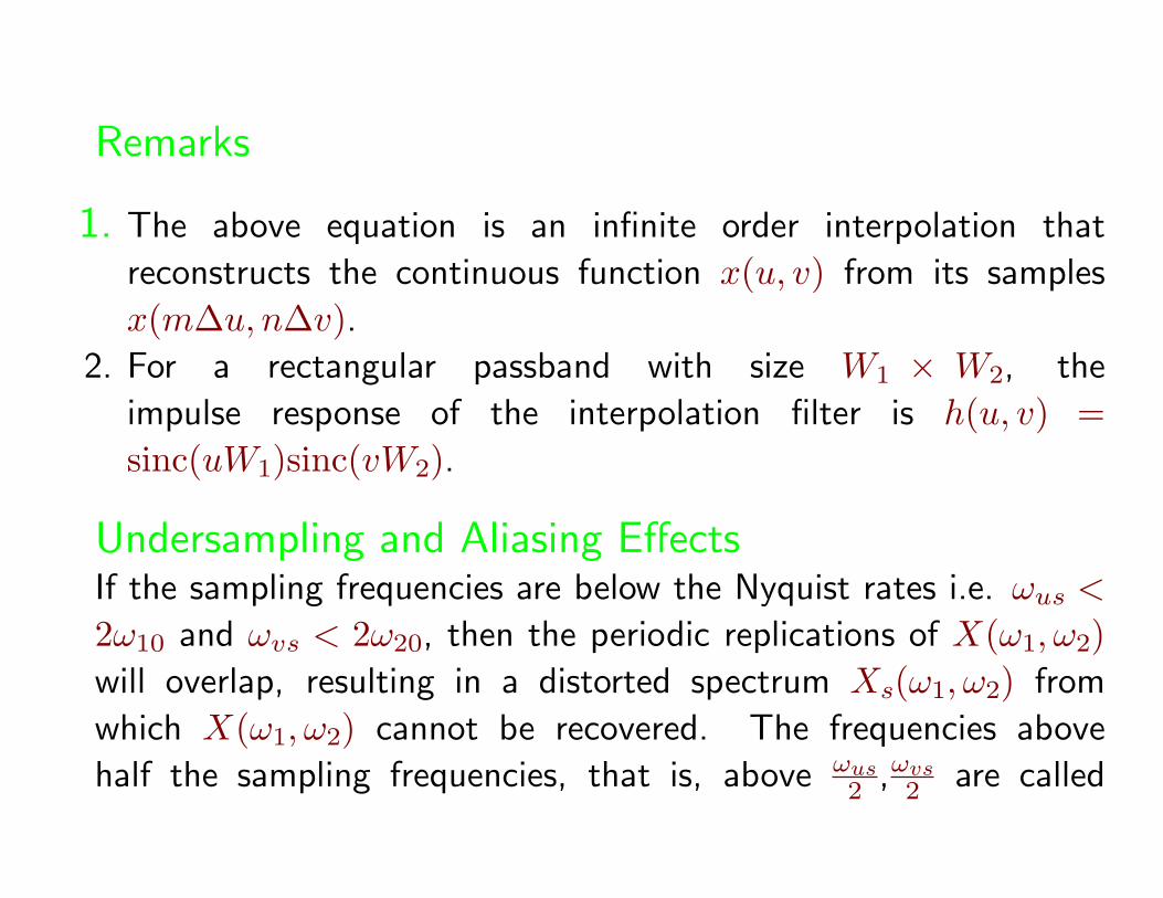
Remarks

1. The above equation is an infinite order interpolation that

reconstructs the continuous function x(u, v) from its samples

x(m∆u, n∆v).2. For a rectangular passband with size W1 × W2, the

impulse response of the interpolation filter is h(u, v) =sinc(uW1)sinc(vW2).

Undersampling and Aliasing EffectsIf the sampling frequencies are below the Nyquist rates i.e. ωus <

2ω10 and ωvs < 2ω20, then the periodic replications of X(ω1, ω2)will overlap, resulting in a distorted spectrum Xs(ω1, ω2) from

which X(ω1, ω2) cannot be recovered. The frequencies above

half the sampling frequencies, that is, above ωus2 ,ωvs

2 are called


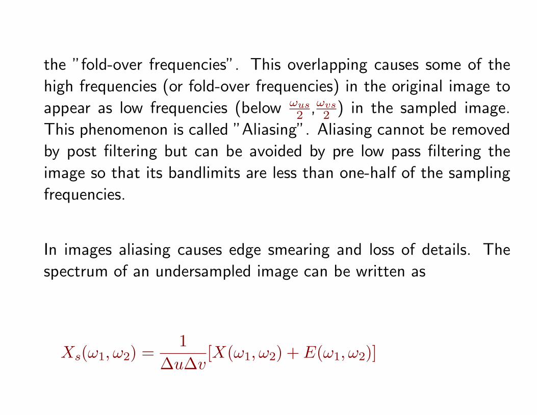
the ”fold-over frequencies”. This overlapping causes some of the

high frequencies (or fold-over frequencies) in the original image to

appear as low frequencies (below ωus2 ,ωvs

2 ) in the sampled image.

This phenomenon is called ”Aliasing”. Aliasing cannot be removed

by post filtering but can be avoided by pre low pass filtering the

image so that its bandlimits are less than one-half of the sampling

frequencies.

In images aliasing causes edge smearing and loss of details. The

spectrum of an undersampled image can be written as

Xs(ω1, ω2) =1

∆u∆v[X(ω1, ω2) + E(ω1, ω2)]


where

E(ω1, ω2) =∑ ∞∑

k, l = −∞(k, l) 6= (0, 0)

X(ω1 − kωus, ω2 − lωvs)

After the filtering with a 2-D LPF

H(ω1, ω2) =

∆u∆v |ω1| ≤ ωus2 , |ω2| ≤ ωvs

2

0 otherwise

we get X(ω1, ω2) = H(ω1, ω2)Xs(ω1, ω2). In the spatial domain,

we get

x(u, v) = x(u, v) + e(u, v)


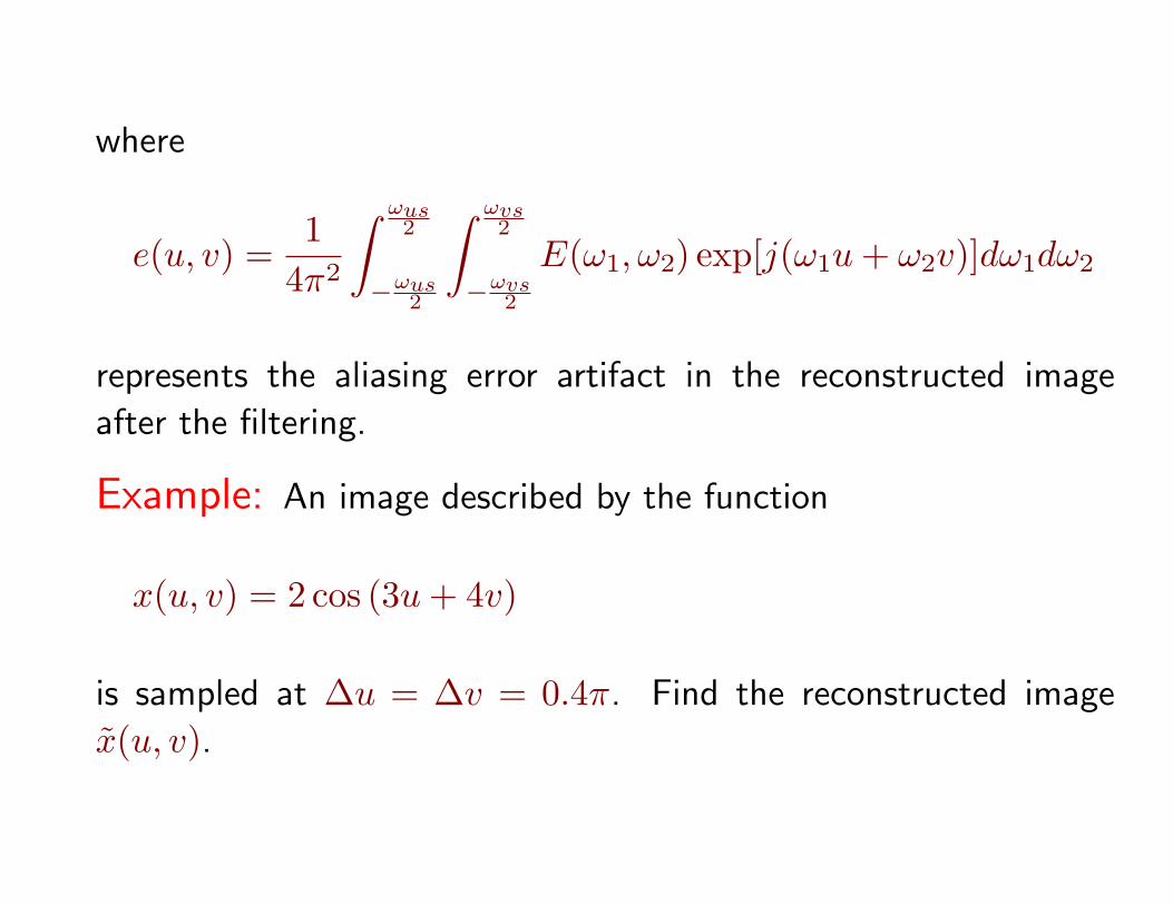
where

e(u, v) =1

4π2

∫ ωus2

−ωus2

∫ ωvs2

−ωvs2

E(ω1, ω2) exp[j(ω1u + ω2v)]dω1dω2

represents the aliasing error artifact in the reconstructed image

after the filtering.

Example: An image described by the function

x(u, v) = 2 cos (3u + 4v)

is sampled at ∆u = ∆v = 0.4π. Find the reconstructed image

x(u, v).


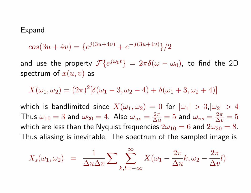
Expand

cos(3u + 4v) = ej(3u+4v) + e−j(3u+4v)/2

and use the property Fejω0t = 2πδ(ω − ω0), to find the 2D

spectrum of x(u, v) as

X(ω1, ω2) = (2π)2[δ(ω1 − 3, ω2 − 4) + δ(ω1 + 3, ω2 + 4)]

which is bandlimited since X(ω1, ω2) = 0 for |ω1| > 3,|ω2| > 4Thus ω10 = 3 and ω20 = 4. Also ωus = 2π

∆u = 5 and ωvs = 2π∆v = 5

which are less than the Nyquist frequencies 2ω10 = 6 and 2ω20 = 8.

Thus aliasing is inevitable. The spectrum of the sampled image is

Xs(ω1, ω2) =1

∆u∆v

∑ ∞∑k,l=−∞

X(ω1 −2π

∆uk, ω2 −

2π

∆vl)


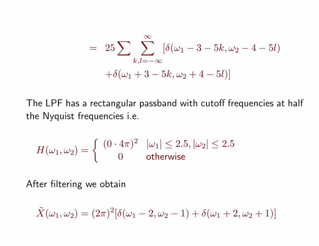
= 25∑ ∞∑

k,l=−∞

[δ(ω1 − 3− 5k, ω2 − 4− 5l)

+δ(ω1 + 3− 5k, ω2 + 4− 5l)]

The LPF has a rectangular passband with cutoff frequencies at half

the Nyquist frequencies i.e.

H(ω1, ω2) =

(0 · 4π)2 |ω1| ≤ 2.5, |ω2| ≤ 2.50 otherwise

After filtering we obtain

X(ω1, ω2) = (2π)2[δ(ω1 − 2, ω2 − 1) + δ(ω1 + 2, ω2 + 1)]


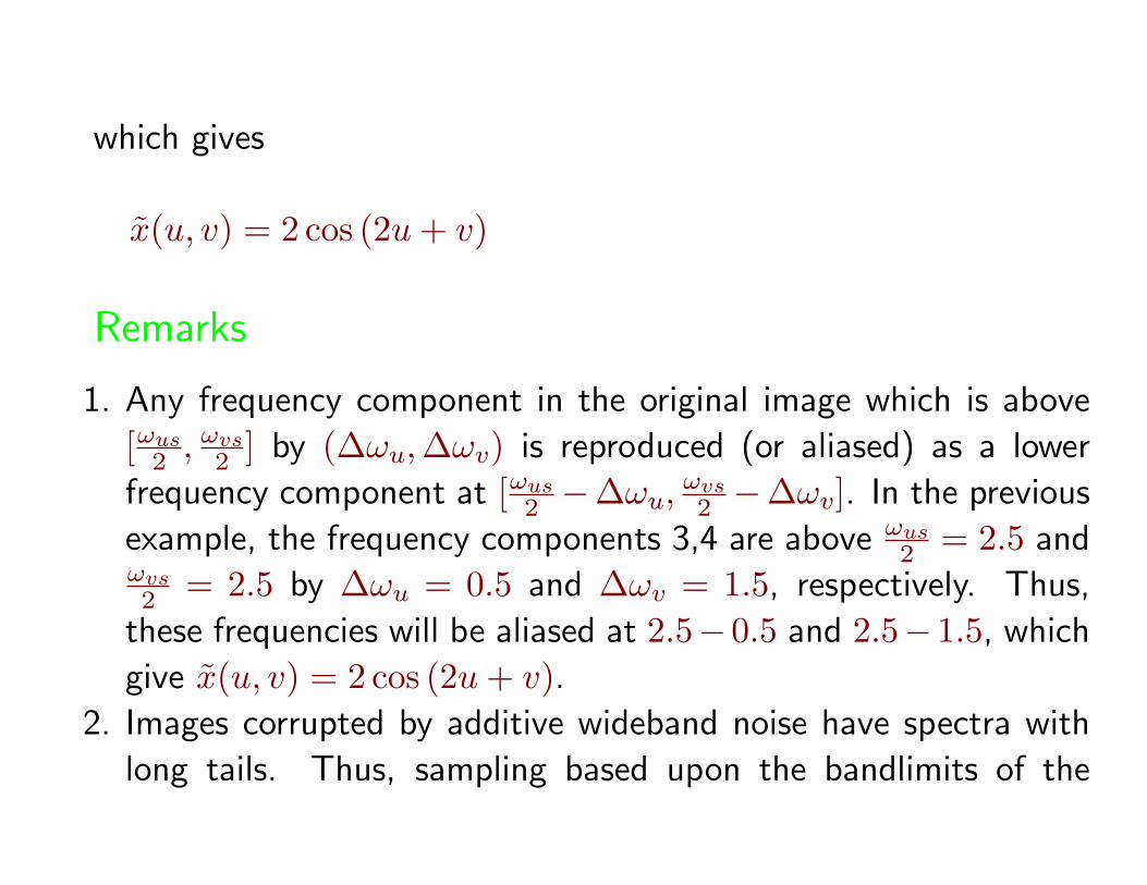
which gives

x(u, v) = 2 cos (2u + v)

Remarks

1. Any frequency component in the original image which is above

[ωus2 , ωvs

2 ] by (∆ωu,∆ωv) is reproduced (or aliased) as a lower

frequency component at [ωus2 −∆ωu, ωvs

2 −∆ωv]. In the previous

example, the frequency components 3,4 are above ωus2 = 2.5 and

ωvs2 = 2.5 by ∆ωu = 0.5 and ∆ωv = 1.5, respectively. Thus,

these frequencies will be aliased at 2.5−0.5 and 2.5−1.5, which

give x(u, v) = 2 cos (2u + v).2. Images corrupted by additive wideband noise have spectra with

long tails. Thus, sampling based upon the bandlimits of the


original image will result in aliasing effects as the tail of the

spectrum will fold-over into the bandlimits of the image. This

obviously causes additional noise in the reconstructed image.

To prevent this problem the image must be prefiltered prior to

sampling.


digital image processing lectures 5 & 6

Documents