DIFFERENTIALS: LINEAR

AND QUADRATIC

APPROXIMATION

By Kenny Abitbol, Sam Mote, and Evan

Kirkland

Introduction of Linear

Approximation

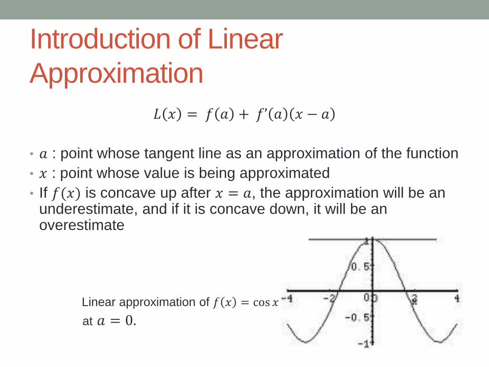
𝐿 𝑥 = 𝑓 𝑎 + 𝑓’ 𝑎 𝑥 − 𝑎

• 𝑎 : point whose tangent line as an approximation of the function

• 𝑥 : point whose value is being approximated

• If 𝑓(𝑥) is concave up after 𝑥 = 𝑎, the approximation will be an underestimate, and if it is concave down, it will be an overestimate

Linear approximation of 𝑓 𝑥 = cos 𝑥

at 𝑎 = 0.

Definition of Linear Approximation

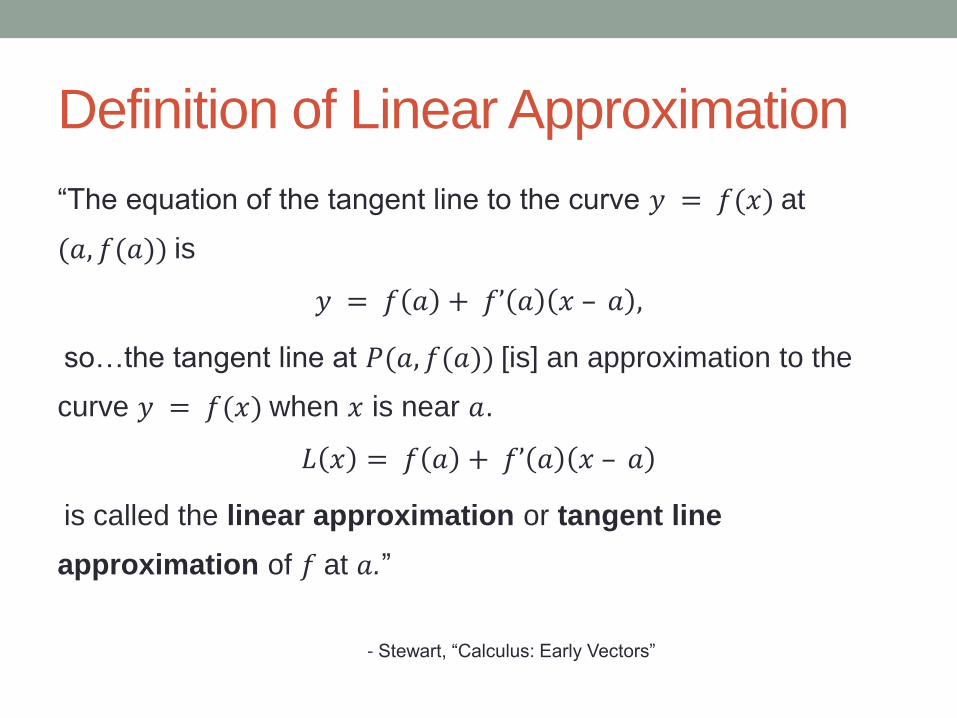
“The equation of the tangent line to the curve 𝑦 = 𝑓(𝑥) at

(𝑎, 𝑓(𝑎)) is

𝑦 = 𝑓 𝑎 + 𝑓’ 𝑎 𝑥 – 𝑎 ,

so…the tangent line at 𝑃(𝑎, 𝑓(𝑎)) [is] an approximation to the

curve 𝑦 = 𝑓(𝑥) when 𝑥 is near 𝑎.

𝐿 𝑥 = 𝑓 𝑎 + 𝑓’ 𝑎 𝑥 – 𝑎

is called the linear approximation or tangent line

approximation of 𝑓 at 𝑎.”

- Stewart, “Calculus: Early Vectors”

Introduction of Quadratic

Approximation

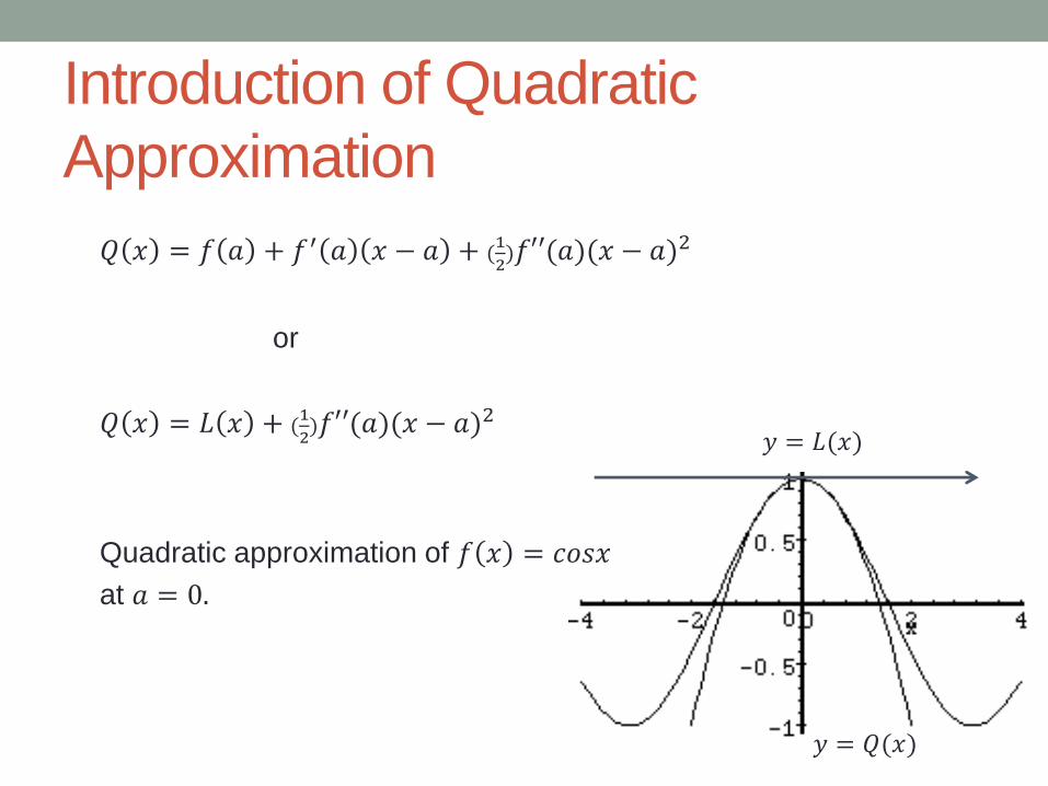
𝑄 𝑥 = 𝑓 𝑎 + 𝑓′ 𝑎 𝑥 − 𝑎 + (1

2)𝑓′′(𝑎)(𝑥 − 𝑎)2

or

𝑄 𝑥 = 𝐿 𝑥 + (1

2)𝑓′′(𝑎)(𝑥 − 𝑎)2

Quadratic approximation of 𝑓 𝑥 = 𝑐𝑜𝑠𝑥

at 𝑎 = 0.

𝑦 = 𝐿(𝑥)

𝑦 = 𝑄(𝑥)

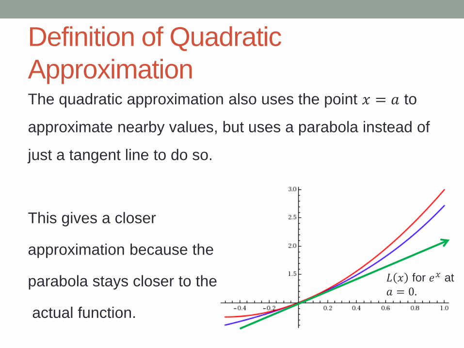
Definition of Quadratic

Approximation The quadratic approximation also uses the point 𝑥 = 𝑎 to

approximate nearby values, but uses a parabola instead of

just a tangent line to do so.

This gives a closer

approximation because the

parabola stays closer to the

actual function.

𝐿 𝑥 for 𝑒𝑥 at

𝑎 = 0.

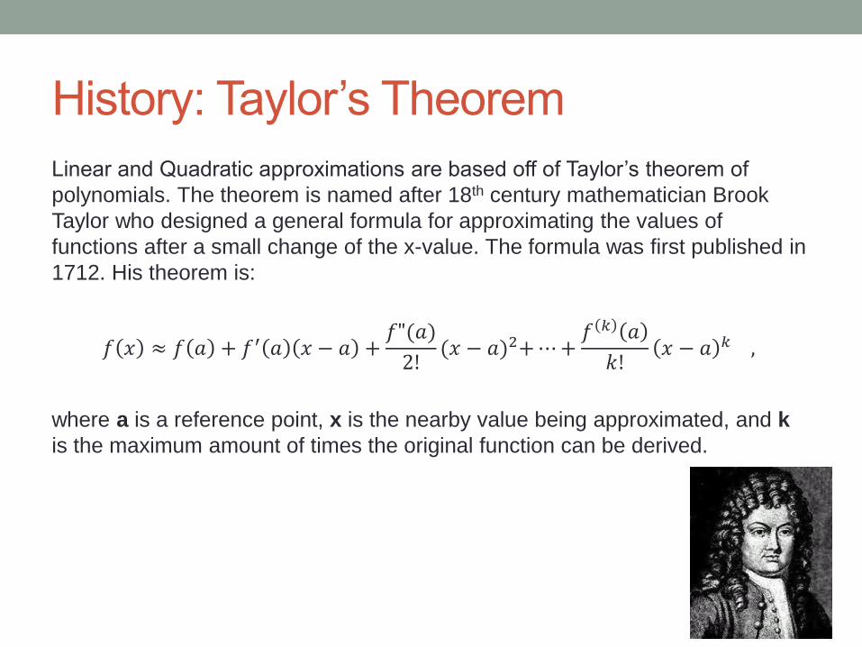
History: Taylor’s Theorem

Linear and Quadratic approximations are based off of Taylor’s theorem of

polynomials. The theorem is named after 18th century mathematician Brook

Taylor who designed a general formula for approximating the values of

functions after a small change of the x-value. The formula was first published in

1712. His theorem is:

𝑓 𝑥 ≈ 𝑓 𝑎 + 𝑓′ 𝑎 𝑥 − 𝑎 +𝑓"(𝑎)

2!(𝑥 − 𝑎)2+ ⋯ +

𝑓 𝑘 𝑎

𝑘!𝑥 − 𝑎 𝑘 ,

where a is a reference point, x is the nearby value being approximated, and k

is the maximum amount of times the original function can be derived.

History: Differentials

• Began in 1680’s

• Bernouli brothers

• Gottfried Wilhelm Leibniz

• Applied to geometry and mechanics

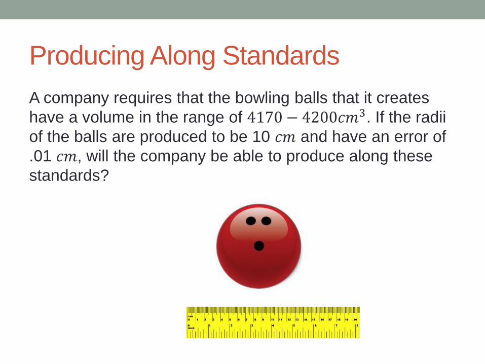
Producing Along Standards

A company requires that the bowling balls that it creates

have a volume in the range of 4170 − 4200𝑐𝑚3. If the radii

of the balls are produced to be 10 𝑐𝑚 and have an error of

.01 𝑐𝑚, will the company be able to produce along these

standards?

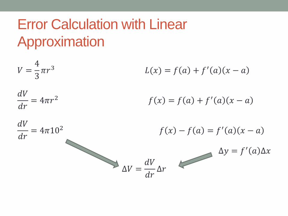
Error Calculation with Linear

Approximation

𝑉 =4

3𝜋𝑟3 𝐿(𝑥) = 𝑓 𝑎 + 𝑓′ 𝑎 𝑥 − 𝑎

𝑑𝑉

𝑑𝑟= 4𝜋𝑟2 𝑓 𝑥 = 𝑓 𝑎 + 𝑓′ 𝑎 𝑥 − 𝑎

𝑑𝑉

𝑑𝑟= 4𝜋102 𝑓 𝑥 − 𝑓 𝑎 = 𝑓′ 𝑎 𝑥 − 𝑎

∆𝑦 = 𝑓′ 𝑎 ∆𝑥

∆𝑉 =𝑑𝑉

𝑑𝑟∆𝑟

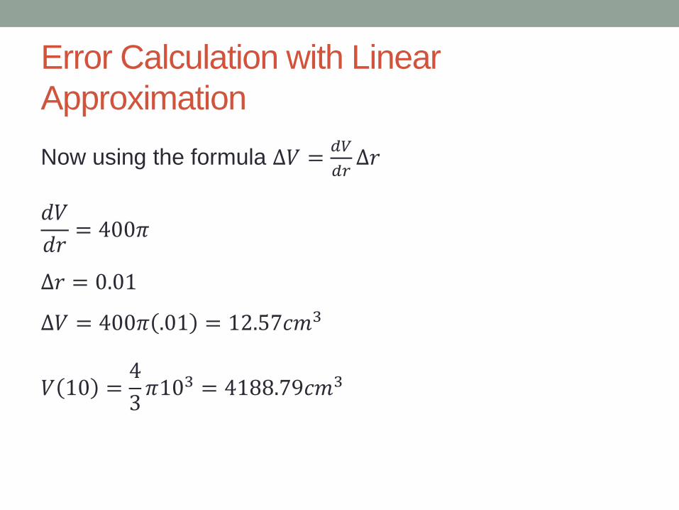
Error Calculation with Linear

Approximation

Now using the formula ∆𝑉 =𝑑𝑉

𝑑𝑟∆𝑟

𝑑𝑉

𝑑𝑟= 400𝜋

∆𝑟 = 0.01

∆𝑉 = 400𝜋 .01 = 12.57𝑐𝑚3

𝑉 10 =4

3𝜋103 = 4188.79𝑐𝑚3

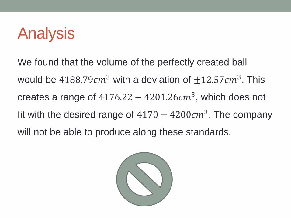
Analysis

We found that the volume of the perfectly created ball

would be 4188.79𝑐𝑚3 with a deviation of ±12.57𝑐𝑚3. This

creates a range of 4176.22 − 4201.26𝑐𝑚3, which does not

fit with the desired range of 4170 − 4200𝑐𝑚3. The company

will not be able to produce along these standards.

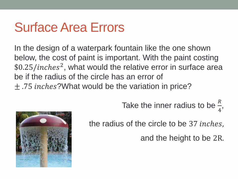
Surface Area Errors

In the design of a waterpark fountain like the one shown

below, the cost of paint is important. With the paint costing

$0.25/𝑖𝑛𝑐ℎ𝑒𝑠2, what would the relative error in surface area

be if the radius of the circle has an error of

± .75 𝑖𝑛𝑐ℎ𝑒𝑠?What would be the variation in price?

Take the inner radius to be 𝑅

4,

the radius of the circle to be 37 𝑖𝑛𝑐ℎ𝑒𝑠,

and the height to be 2R.

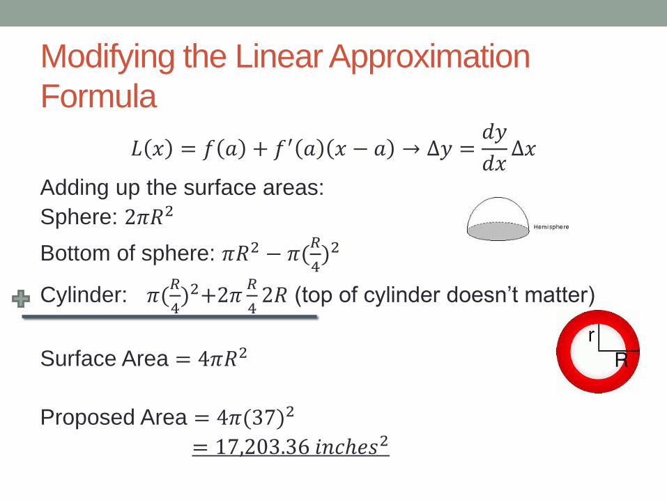
Modifying the Linear Approximation

Formula

𝐿 𝑥 = 𝑓 𝑎 + 𝑓′ 𝑎 𝑥 − 𝑎 → ∆𝑦 =𝑑𝑦

𝑑𝑥∆𝑥

Adding up the surface areas:

Sphere: 2𝜋𝑅2

Bottom of sphere: 𝜋𝑅2 − 𝜋(𝑅

4)2

Cylinder: 𝜋(𝑅

4)2+2𝜋

𝑅

42𝑅 (top of cylinder doesn’t matter)

Surface Area = 4𝜋𝑅2

Proposed Area = 4𝜋(37)2

= 17,203.36 𝑖𝑛𝑐ℎ𝑒𝑠2

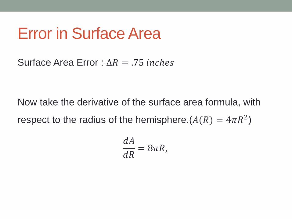
Error in Surface Area

Surface Area Error : ∆𝑅 = .75 𝑖𝑛𝑐ℎ𝑒𝑠

Now take the derivative of the surface area formula, with

respect to the radius of the hemisphere.(𝐴(𝑅) = 4𝜋𝑅2)

𝑑𝐴

𝑑𝑅= 8𝜋𝑅,

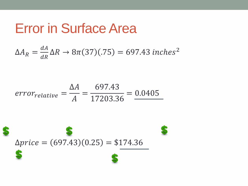
Error in Surface Area

∆𝐴𝑅 =𝑑𝐴

𝑑𝑅∆𝑅 → 8𝜋 37 .75 = 697.43 𝑖𝑛𝑐ℎ𝑒𝑠2

𝑒𝑟𝑟𝑜𝑟𝑟𝑒𝑙𝑎𝑡𝑖𝑣𝑒 =∆𝐴

𝐴=

697.43

17203.36= 0.0405

∆𝑝𝑟𝑖𝑐𝑒 = 697.43 0.25 = $174.36

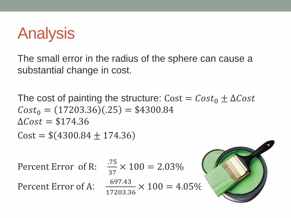
Analysis

The small error in the radius of the sphere can cause a

substantial change in cost.

The cost of painting the structure: Cost = 𝐶𝑜𝑠𝑡0 ± ∆𝐶𝑜𝑠𝑡

𝐶𝑜𝑠𝑡0 = 17203.36 .25 = $4300.84 ∆𝐶𝑜𝑠𝑡 = $174.36

Cost = $ 4300.84 ± 174.36

Percent Error of R: .75

37× 100 = 2.03%

Percent Error of A: 697.43

17203.36× 100 = 4.05%

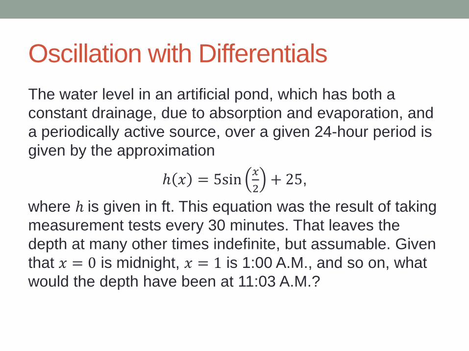
Oscillation with Differentials

The water level in an artificial pond, which has both a

constant drainage, due to absorption and evaporation, and

a periodically active source, over a given 24-hour period is

given by the approximation

ℎ 𝑥 = 5sin𝑥

2+ 25,

where ℎ is given in ft. This equation was the result of taking

measurement tests every 30 minutes. That leaves the

depth at many other times indefinite, but assumable. Given

that 𝑥 = 0 is midnight, 𝑥 = 1 is 1:00 A.M., and so on, what

would the depth have been at 11:03 A.M.?

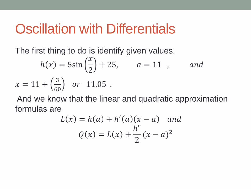
Oscillation with Differentials

The first thing to do is identify given values.

ℎ 𝑥 = 5sin𝑥

2+ 25, 𝑎 = 11 , 𝑎𝑛𝑑

𝑥 = 11 +3

60 𝑜𝑟 11.05 .

And we know that the linear and quadratic approximation

formulas are

𝐿 𝑥 = ℎ 𝑎 + ℎ′ 𝑎 𝑥 − 𝑎 𝑎𝑛𝑑

𝑄 𝑥 = 𝐿 𝑥 +ℎ"

2(𝑥 − 𝑎)2

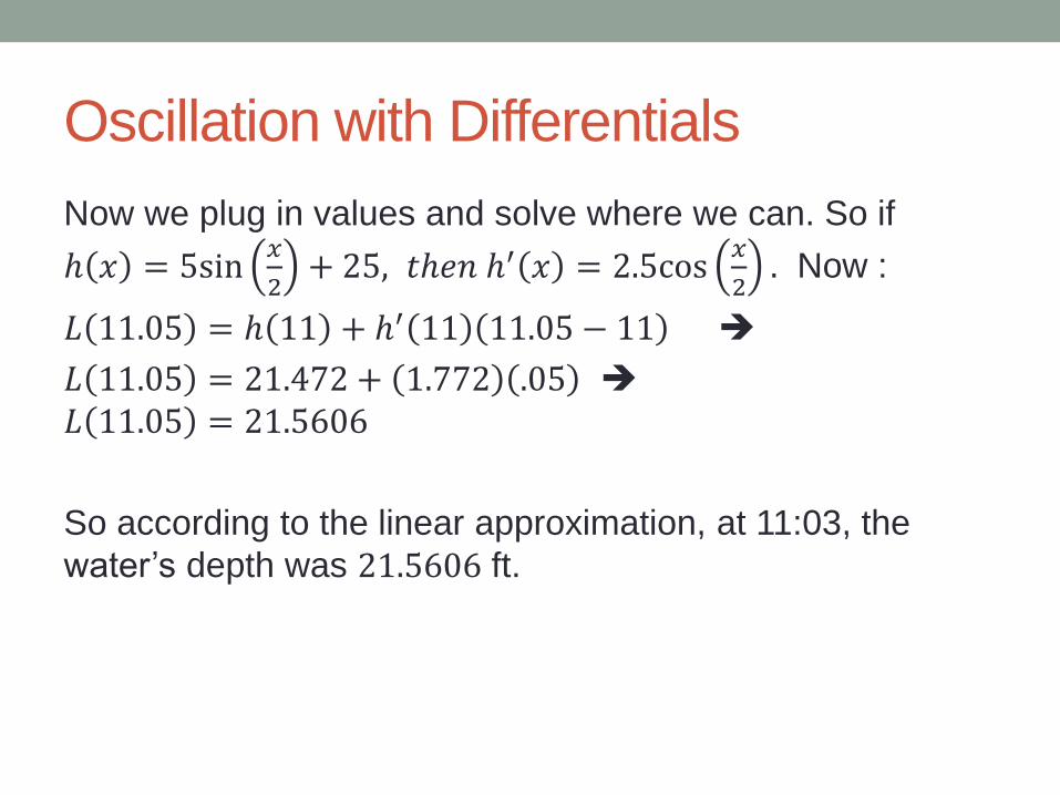
Oscillation with Differentials

Now we plug in values and solve where we can. So if

ℎ 𝑥 = 5sin𝑥

2+ 25, 𝑡ℎ𝑒𝑛 ℎ′ 𝑥 = 2.5cos

𝑥

2. Now :

𝐿 11.05 = ℎ 11 + ℎ′ 11 11.05 − 11

𝐿 11.05 = 21.472 + 1.772 .05

𝐿 11.05 = 21.5606

So according to the linear approximation, at 11:03, the

water’s depth was 21.5606 ft.

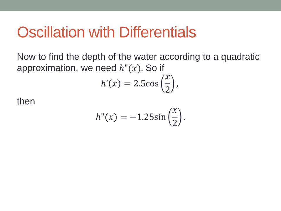
Oscillation with Differentials

Now to find the depth of the water according to a quadratic

approximation, we need ℎ"(𝑥). So if

ℎ’ 𝑥 = 2.5cos 𝑥

2,

then

ℎ"(𝑥) = −1.25sin 𝑥

2.

Oscillation with Differentials

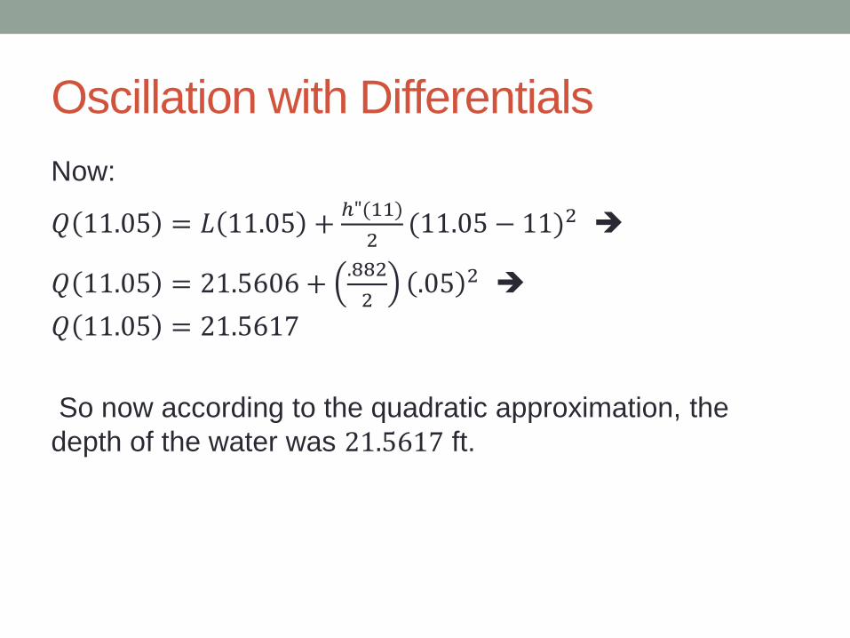
Now:

𝑄 11.05 = 𝐿 11.05 +ℎ"(11)

2(11.05 − 11)2

𝑄 11.05 = 21.5606 +.882

2.05 2

𝑄 11.05 = 21.5617

So now according to the quadratic approximation, the

depth of the water was 21.5617 ft.

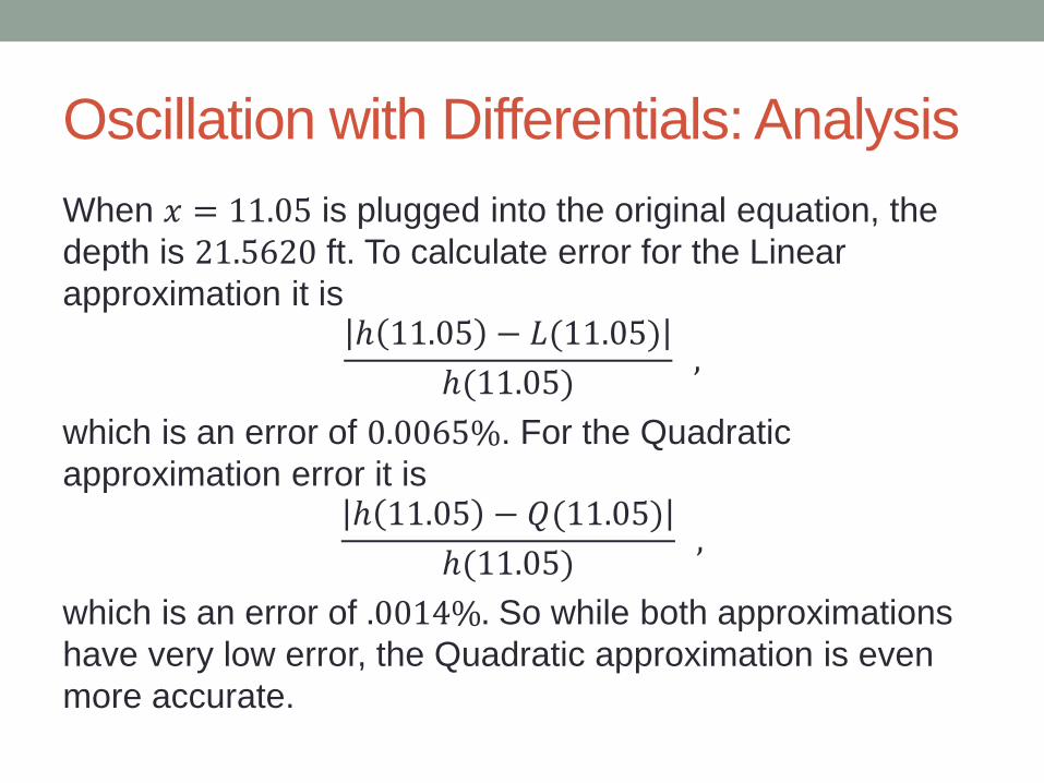
Oscillation with Differentials: Analysis

When 𝑥 = 11.05 is plugged into the original equation, the

depth is 21.5620 ft. To calculate error for the Linear

approximation it is ℎ 11.05 − 𝐿(11.05)

ℎ(11.05) ,

which is an error of 0.0065%. For the Quadratic

approximation error it is ℎ 11.05 − 𝑄(11.05)

ℎ(11.05) ,

which is an error of .0014%. So while both approximations

have very low error, the Quadratic approximation is even

more accurate.

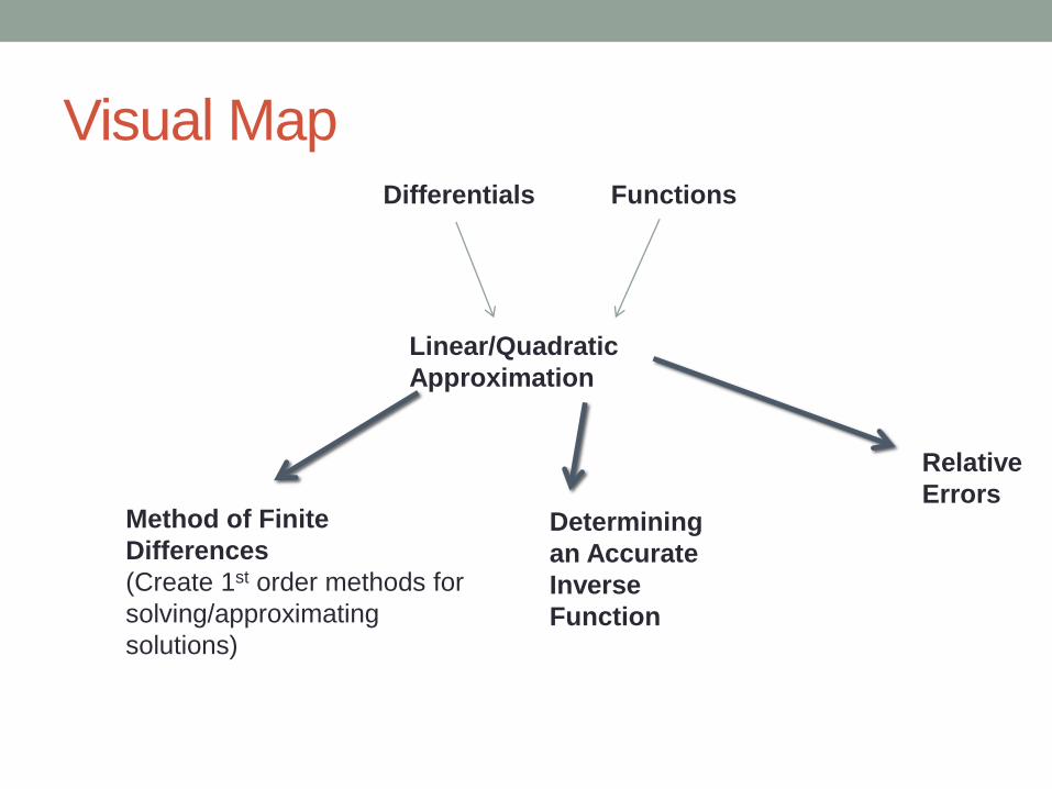
Visual Map Differentials Functions

Linear/Quadratic

Approximation

Method of Finite

Differences

(Create 1st order methods for

solving/approximating

solutions)

Determining

an Accurate

Inverse

Function

Relative

Errors

Common Mistakes

• Omission of 1

2 in equation for quadratic approximation

• (𝑥 − 𝑎) is used instead of (𝑥 − 𝑎)2 in the quadratic

approximation

• Chain rule forgotten when taking derivatives

• Plug 𝑓′(𝑥) instead of 𝑓′(𝑎) into linear or quadratic

approximation

References

"Linear Approximation." Wikipedia.org. 6 November 2012. Web. 3 June 2012.

<http://en.wikipedia.org/wiki/Linear_approximation>.

Stewart, James. "Calculus: Early Vectors." 1st ed. Pacific Grove: Brooks/Cole, 1999.

Print.

"Taylor's Theorem." Wikipedia.org. 6 November 2012. Web. 5 November 2012.

<http://en.wikipedia.org/wiki/Taylor's_theorem>.