differentiable manifolds -...
TRANSCRIPT
Chapter 24
Differentiable Manifolds
We have reached a stage for which it is beneficial to take on board the theory
of manifolds. This more abstract theory is a vehicle in which the definitions of
Chapter 9 for Euclidean spaces extend in a natural way. The resulting concepts
will provide us with a framework in which to pursue the intrinsic study of
surfaces begun in Chapter 17.
The modern concept of a differentiable manifold, due to Weyl1 (see [Weyl]),
did not appear until the early twentieth century. A manifold , generally speaking,
is a topological space which resembles Euclidean space locally. A differentiable
manifold is a manifold M for which this resemblance is sharp enough to allow
partial differentiation and consequently all the features of differential calculus
on M. The study of differentiable manifolds involves topology, since differen-
tiability implies continuity, but metric properties of Euclidean space are not a
priori included. In this chapter, we define the notion of differentiable manifold
and some of the standard apparatus associated with it. Metrics and distances
are discussed in the following two chapters.
The set Rn of n-tuples of real numbers is not only a vector space, but also
a topological space, and the vector operations are continuous with respect to
the topology. In addition, there is the notion of differentiability of real-valued
functions on Rn: we say that f : Rn → R is differentiable provided that the
partial derivatives
∂i1+···+irf
∂ui11 . . . ∂u
irr
1
Hermann Klaus Hugo Weyl (1885–1955). German mathematician, who
together with E. Cartan created the basis for the modern theory of Lie
groups and their representations. With his application of group theory to
quantum mechanics, he set up the modern theory of the subject. He was
professor in Zurich and Gottingen. From 1933 until he retired in 1952, he
worked at the Institute of Advanced Study at Princeton.
809

810 CHAPTER 24. DIFFERENTIABLE MANIFOLDS
of all orders exist. Such functions are called C∞ functions . They contrast
with, on the one hand, the Ck functions (the functions which have continuous
partial derivatives whenever i1 + · · · + ir 6 k) and, on the other hand, the real
analytic functions (functions which have convergent power series). If we denote
these respective classes by C∞(Rn), Ck(Rn), Cω(Rn), then we have the strict
inclusions
Cω(Rn) ⊂ C∞(Rn) ⊂ Ck(Rn).
We choose to base our definitions on the class of C∞ functions; use of Ck
requires too complicated an approach, and use of Cω is too restrictive.
In Section 24.1, we give the definition of differentiable manifold and describe
some simple examples. The n-dimensional sphere is made into a differentiable
manifold by introducing maps that generalize the stereographic map studied in
Sections 8.6 and 22.3. The algebra F(M) of C∞ functions on a differentiable
manifold is described in Section 24.2. The ensuing definitions generalize those
already given in Chapter 12 for functions on and between surfaces. The tangent
space to a differentiable manifold is defined in Section 24.3, and derives from
the analogous Section 9.3. Maps between differentiable manifolds are studied
in Section 24.4, and vector fields and tensor fields in Sections 24.5 and 24.6.
We shall assume that the reader is familiar with all the basic information
about calculus of several variables, including the implicit function theorem and
existence theorems for ordinary differential equations. This material can be
found in, for example, [Spiv].
24.1 The Definition of a Differentiable Manifold
Recall the definition of the natural coordinate functions of Rn given on page 273;
these are the mappings ui : Rn → R defined by
ui(p1, . . . , pn) = pi
for i = 1, . . . , n, and we shall resolutely distinguish the functions ui and the
numbers pi. A function Ψ: Rm → Rn is differentiable, continuous or linear if
and only if each ui ◦ Ψ is differentiable, continuous or linear, respectively. This
is consistent with Definition 9.7 on page 268.
We now make precise the ‘local resemblance’ referred to on the previous
page.
Definition 24.1. A patch on a topological space M is a pair (x,U), where U is
an open subset of Rn and
x : U −→ x(U) ⊂ M
is a homeomorphism of U onto an open set x(U) of M.

24.1. DEFINITION OF DIFFERENTIABLE MANIFOLD 811
Here x is called the local homeomorphism of the patch, and x(U) the coordinate
neighborhood. Frequently, we refer to ‘the patch x’ when the domain U is
understood. Let
xi = ui ◦ x−1 : x(U) −→ R(24.1)
for i = 1, . . . , n. Then xi is called the ith coordinate function and (x1, . . . , xn) is
called a system of local coordinates for M. The coordinate functions x1, . . . , xn
contain the same information as the local homeomorphism x. Often, we write
x−1 = (x1, . . . , xn), with the meaning that
x−1(p) =(x1(p), . . . , xn(p)
)
for all p ∈ x(U).
We are now ready to define the notion of differentiable manifold. Intuitively,
the idea is this: in studying the geography of the earth, it is a great convenience
to use geographical maps or patches instead of examining the earth directly.
A collection of geographical maps that covers the earth is called an atlas, and
it gives a complete picture of the earth. Roughly, we shall follow the same
procedure with differentiable manifolds.
Definition 24.2. An atlas A on a topological space M is a collection of patches
on M such that all the patches map from open subsets of the same Euclidean
space Rn into M, and M is the union of all the x(U)’s such that (x,U) ∈ A.
A topological space M equipped with an atlas is called a topological manifold.
Let A be an atlas on a topological space M. Notice that if (x,U) and (y,V)
are two patches in A such that x(U) ∩ y(V) = W is a nonempty subset of M,
then the map
x−1 ◦ y : y−1(W) −→ x−1(W)(24.2)
is a homeomorphism between open subsets of Rn. We call x−1 ◦ y a change of
coordinates. We are now in a position to state
Definition 24.3. A differentiable manifold is a paracompact topological space M
equipped with an atlas A such that for any two patches (x,U), (y,V) in A with
x(U) ∩ y(V) = W nonempty, the change of coordinates (24.2) is differentiable
(that is, of class C∞) in the ordinary Euclidean sense. The dimension of the
manifold M (denoted by dimM) is the number n in Definition 24.2.
Remarks
(1) Topological terms applied to a manifold apply to its underlying topological
space; for example, we shall assume that a given differentiable manifold
is connected, unless stated otherwise. Manifolds share many of the local
properties of Euclidean space Rn, for example, local connectedness and

812 CHAPTER 24. DIFFERENTIABLE MANIFOLDS
local compactness, but the paracompact assumption needs to be added.
Strictly speaking, the hypothesis of Hausdorff should also be added in the
definition to exclude certain pathological examples. The exact meaning of
these words is not important for us, but their definitions can be found in
any book on general topology, such as [Kelley].
(2) A function of n complex variables is called holomorphic if it is so in each
variable separately (see page 721), and in this case it is expandable in a
complex power series in a neighborhood of each point where it is defined.
The definition of complex manifold is the same as that of a differentiable
manifold, except that the local homeomorphisms are required to map from
open subsets of Cn, and the changes of coordinates (24.2) are required
to be holomorphic rather than C∞. Any such complex manifold is, in
particular, a real manifold of dimension 2n.
Implicitly associated with A is a possibly larger atlas, which is a theoretical
nicety that is needed to declare when two manifolds are really the same.
Definition 24.4. The completion A of an atlas A is the collection
A ={
(x,U) | x−1◦ y and y−1◦ x are differentiable for all (y,V) ∈ A}.
We say that an atlas A is complete if it coincides with its completion.
We do not distinguish between differentiable manifolds (M,A1) and (M,A2)
when the atlases A1 and A2 have the same completion. When we speak of a
‘differentiable manifold M’, we shall mean a differentiable manifold M equipped
with a specific complete atlas.
There are two simple but important ways to construct new manifolds from
old.
Definition 24.5. Let M be a differentiable manifold defined by a complete atlas
A, and let V be an open subset of M. Define
A |V ={
(x,U) ∈ A | x(U) ⊆ V}.
Evidently, A |V is an atlas of V. We call V equipped with the atlas A(V ) an
open submanifold of M.
Definition 24.6. Let M1 and M2 be differentiable manifolds of dimensions n1
and n2 defined by atlases A1 and A2. If (x,U) is in A1 and (y,V) is in A2, we
define x × y : U × V → M1 ×M2 by
(x × y)(p,q) =(x(p),y(q)
).

24.1. DEFINITION OF DIFFERENTIABLE MANIFOLD 813
Then M1 ×M2 equipped with the completion of the atlas
{(x × y, U × V) | (x,U) ∈ A1, (y,V) ∈ A2
}
is a differentiable manifold of dimension n1 + n2, called the product of M1
and M2.
For the proof that M1×M2 is actually a differentiable manifold, see Exercise 1.
Examples of Differentiable Manifolds
The Euclidean space Rn is made into a differentiable manifold as follows. Let
1 : Rn → Rn denote the identity map
(u1, , . . . , un): Rn −→ R
n.
Then (1,Rn) constitutes an atlas for Rn all by itself. This formalizes the fact
that the notion of manifold is a generalization of Euclidean space.
The n-dimensional sphere represents an example where the concept of atlas
is essential. Let a > 0 and put
Sn(a) =
{(t0, . . . , tn) ∈ R
n+1
∣∣∣∣n∑
j=0
t2j = a2
}.
We shall make Sn(a) into a differentiable manifold by defining an atlas
A ={
(north,Rn), (south,Rn)},
where north and south are the ‘stereographic injections’. Analytically these are
patches
north : Rn −→ Sn(a) \ {n} and south : R
n −→ Sn(a) \ {s},
where n = (a, 0, . . . , 0) is the ‘north pole’, and s = (−a, 0, , . . . , 0) is the ‘south
pole’. They are defined by setting
north = (Φ0, . . . ,Φn), south = (Ψ0, . . . ,Ψn),
where
Φ0 = −Ψ0 = a
−a2 +
n∑
j=1
u2j
a2 +n∑
j=1
u2j
, and Φk = Ψk =
2a2uk
a2 +n∑
j=1
u2j
for k = 1, . . . , n. In the special case n = 2 and a = 1, north coincides with Υ
on page 250. It is also the inverse of the stereographic projection described by

814 CHAPTER 24. DIFFERENTIABLE MANIFOLDS
Definition 22.19 and Figure 22.2 on page 730 with (u1, u2) a point of the equa-
torial plane R2; south is obtained using straight lines passing through (0, 0,−a)
instead of (a, 0, 0). It is easily verified that north and south are injective, and
the compositions north ◦ south−1 and south ◦ north−1 are differentiable.
To conclude this subsection, we insert a result that provides a whole host of
examples.
Lemma 24.7. A regular surface M in Rn is a differentiable manifold.
Proof. A regular surface in Rn was defined on page 297. For the atlas of M we
choose the regular injective patches on M. Corollary 10.30, page 300, implies
that each change of coordinates is differentiable. Hence M is a differentiable
manifold.
24.2 Differentiable Functions on Manifolds
Differentiable manifolds are locally like Euclidean space. For their study it will
be important to transfer to manifolds as much of the differential calculus of
Euclidean space as we can. First on the agenda is the notion of differentia-
bility for real-valued functions on a differentiable manifold. The definition of
this notion is almost the same as the corresponding definition that we gave on
page 301.
Definition 24.8. Let f : W → R be a function defined on an open subset W
of a differentiable manifold M. We say that f is differentiable at p ∈ W,
provided that for some patch x : U → M with U ⊂ Rn and p ∈ x(U) ⊂ W, the
composition f ◦ x : U → R is differentiable (in the ordinary Euclidean sense) at
x−1(p). If f is differentiable at all points of W, we say that f is differentiable
on W.
This definition illustrates the force behind the definition of differentiable
manifold. One might think that it should be necessary to require that f ◦ x be
differentiable for every patch (x,U) in the atlas of M. However, this fact is a
consequence of the definition:
Lemma 24.9. The definition of differentiability of a real-valued function on a
differentiable manifold does not depend on the choice of patch.
Proof. If (x,U) and (y,V) are patches on a manifold M, then the change of
coordinates x−1 ◦ y is differentiable by the definition of differentiable manifold.
We can write f ◦ y as
f ◦ y = (f ◦ x) ◦ (x−1 ◦ y).
Since the composition of the Euclidean-differentiable functions is differentiable,
the differentiability of f ◦x implies the differentiability of f ◦y, and conversely.

24.2. DIFFERENTIABLE FUNCTIONS 815
Next, we consider the totality of differentiable functions on a differentiable
manifold and define some algebraic structure on it.
Definition 24.10. Let M be a differentiable manifold. We put
F(M) = { f : M → R | f is differentiable } .
We call F(M) the algebra of realvalued differentiable functions M.
For a, b ∈ R and f, g ∈ F(M) the functions af + bg and fg are defined by
(af + bg)(x) = af(x) + bg(x) and (fg)(x) = f(x)g(x)
for x ∈ M. Also, we identify any a ∈ R with the constant function a given by
a(x) = a for x ∈ M.
Let us note some of the algebraic properties of F(M).
Lemma 24.11. Let M be a differentiable manifold. Then F(M) is a commu-
tative ring with identity and an algebra over the real numbers R.
Proof. Let f, g ∈ F(M) and a, b ∈ R. If (x,U) is a patch on M, then f ◦x and
g◦x are differentiable in the ordinary Euclidean sense; hence a(f◦x)+b(g◦x) and
(f ◦x)(g◦x) are Euclidean differentiable. It follows easily that both af+bg and
fg are differentiable. Also, constant functions are differentiable, and the identity
of the ring F(M) is 1 ∈ R. Associativity, commutativity and distributivity are
easy to prove.
Note also that if f ∈ F(M) is never zero, then 1/f ∈ F(M).
It will be important to know when we can extend a real-valued function on
an open set of M to a function that is differentiable on all of M.
Lemma 24.12. Let M be a differentiable manifold, and let p ∈ M. If W is
an open neighborhood of p, then there exist a function k ∈ F(M) and open sets
P and Q such that p ∈ P ⊂ M \Q ⊂ W and
(i) 0 6 k(x) 6 1 for x ∈ M;
(ii) k(x) = 1 for x ∈ P ;
(iii) k(x) = 0 for x ∈ Q.
Proof. For c > 0 let
Bc =
{(p1, . . . , pn) ∈ R
n
∣∣∣∣n∑
j=1
p2j < c
}.
816 CHAPTER 24. DIFFERENTIABLE MANIFOLDS
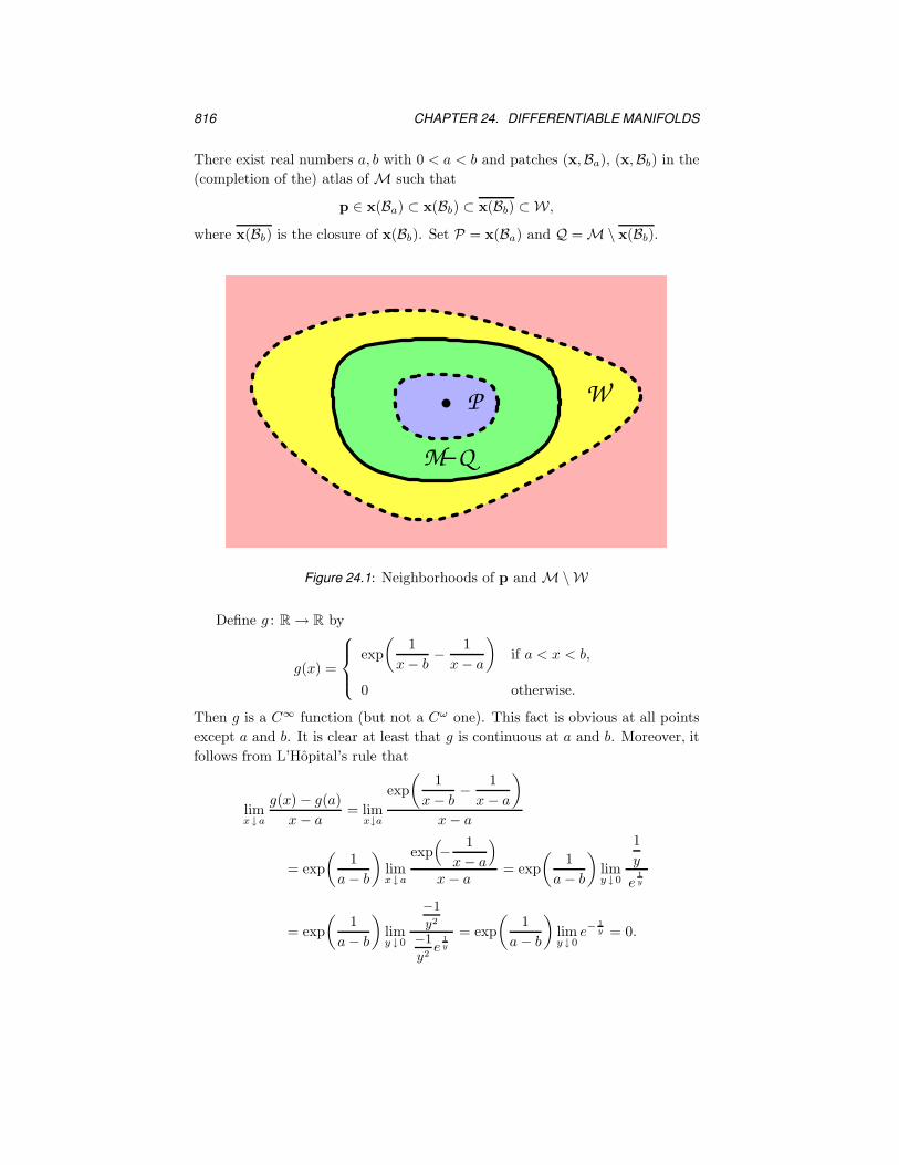
There exist real numbers a, b with 0 < a < b and patches (x,Ba), (x,Bb) in the
(completion of the) atlas of M such that
p ∈ x(Ba) ⊂ x(Bb) ⊂ x(Bb) ⊂ W ,
where x(Bb) is the closure of x(Bb). Set P = x(Ba) and Q = M\ x(Bb).
WP
M-Q
Figure 24.1: Neighborhoods of p and M\W
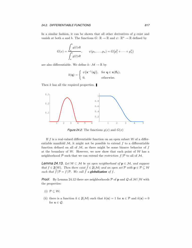
Define g : R → R by
g(x) =
exp
(1
x− b−
1
x− a
)if a < x < b,
0 otherwise.
Then g is a C∞ function (but not a Cω one). This fact is obvious at all points
except a and b. It is clear at least that g is continuous at a and b. Moreover, it
follows from L’Hopital’s rule that
limx↓a
g(x) − g(a)
x− a= lim
x↓a
exp
(1
x− b−
1
x− a
)
x− a
= exp
(1
a− b
)limx↓a
exp(−
1
x− a
)
x− a= exp
(1
a− b
)limy ↓0
1
y
e1
y
= exp
(1
a− b
)limy ↓0
−1
y2
−1
y2e
1
y
= exp
(1
a− b
)limy ↓0
e−1
y = 0.
24.2. DIFFERENTIABLE FUNCTIONS 817
In a similar fashion, it can be shown that all other derivatives of g exist and
vanish at both a and b. The functions G : R → R and ψ : Rn → R defined by
G(x) =
∫ b
x
g(t)dt
∫ b
a
g(t)dt
, ψ(p1, . . . , pn) = G(p21 + · · · + p2
n
)
are also differentiable. We define k : M → R by
k(q) =
{ψ(x−1(q)
), for q ∈ x(Bb),
0, otherwise.
Then k has all the required properties.
1 2 3 4 5 6
0.1
0.2
0.3
1 2 3 4 5
0.2
0.4
0.6
0.8
1
Figure 24.2: The functions g(x) and G(x)
If f is a real-valued differentiable function on an open subset W of a differ-
entiable manifold M, it might not be possible to extend f to a differentiable
function defined on all of M, as there might be some bizarre behavior of f
at the boundary of W . However, we now show that each point of W has a
neighborhood P such that we can extend the restriction f |P to all of M.
Lemma 24.13. Let W ⊂ M be an open neighborhood of p ∈ M, and suppose
that f ∈ F(W). Then there exist f ∈ F(M) and an open set P with p ∈ P ⊆ W
such that f |P = f |P. We call f a globalization of f .
Proof. By Lemma 24.12 there are neighborhoods P of p and Q of M\W with
the properties:
(i) P ⊆ W;
(ii) there is a function k ∈ F(M) such that k(x) = 1 for x ∈ P and k(x) = 0
for x ∈ Q.
818 CHAPTER 24. DIFFERENTIABLE MANIFOLDS
Define f : M → R by
f(q) =
(kf)(q) for q ∈ W ,
0 for q ∈ M \W .
Then f ∈ F(M), and on P we have f = kf = f.
The coordinate functions (24.1) are elements of F(x(U)). By applying Lemma
24.13 to the monomials (xi)m, we see that F(M) is infinite-dimensional. By
contrast, the analogs of Lemmas 24.12 and 24.13 are false for Cω functions.
Having defined the notion of real-valued differentiable function on a differ-
entiable manifold, we are ready to define what it means for a map between
manifolds to be differentiable.
Definition 24.14. Let M,N be differentiable manifolds, and let Ψ: M → N
be a map. We say that Ψ is differentiable provided y−1 ◦ Ψ ◦ x is differentiable
for every patch (x,U) in the atlas of M and every patch (y,V) in the atlas of
N , where the compositions are defined. A diffeomorphism between manifolds M
and N is a differentiable map Φ: M → N which has a differentiable inverse
Φ−1 : N → M. If such a map Φ exists, M and N are said to be diffeomorphic.
A map Ψ: M → N is called a local diffeomorphism provided each p ∈ M has a
neighborhood W such that Ψ |W : W → Ψ(W) is a diffeomorphism.
The following lemma is an easy consequence of the definitions and the fact
that the corresponding lemma for Rn is known.
Lemma 24.15. Suppose MΦ→ N
Ψ→ P are differentiable maps between differ-
entiable manifolds. Then the composition Ψ ◦Φ: M → P is differentiable. If Φ
and Ψ are diffeomorphisms, then so is Ψ ◦ Φ and
(Ψ ◦ Φ)−1 = Φ−1 ◦ Ψ−1.
The coordinates (24.1) are examples of differentiable functions x(U) → R.
Moreover,
Lemma 24.16. Let M be an n-dimensional differentiable manifold, and let
x : U → M be a patch. Write x−1 = (x1, . . . , xn). Then
(i) x is a differentiable mapping between the manifolds U and M;
(ii) x−1 : x(U) → Rn is differentiable;
Proof. Let 1 : Rn → Rn be the identity map. For each patch (y,V) in A, the
maps y−1 ◦x ◦1 and 1 ◦x−1 ◦y are Rn-differentiable. By definition x and x−1,
considered as maps between the manifolds U and M, are differentiable.

24.3. TANGENT VECTORS 819
A differentiable map between manifolds induces a correspondence between
the algebras of differentiable functions on each manifold.
Lemma 24.17. Let Φ: M → N be a differentiable mapping between manifolds.
Then f ∈ F(N ) implies f ◦ Φ ∈ F(M).
Proof. Let (x,U) be a patch on M and (y,V) a patch on N . By hypothesis,
f ◦ y : V → R and y−1 ◦ Φ ◦ x is differentiable. Hence the composition
f ◦ Φ ◦ x = (f ◦ y) ◦ (y−1 ◦ Φ ◦ x)
is differentiable. Since this is true for every patch (x,U) in the atlas of M, it
follows that f ◦ Φ is differentiable.
24.3 Tangent Vectors on Manifolds
By their very nature differentiable manifolds are ‘curved’ spaces, and they can
be very complicated objects to study. In comparison, a vector space is much
simpler. But a vector space has a great deal of structure that facilitates the study
of differentiable manifolds. In this section, we define the notion of tangent space
to a differentiable manifold M at a point p ∈ M. It can be thought of as the
best linear approximation to M at p.
The notion of a vector tangent to a curve or surface in Rn is intuitively clear,
as we have seen in Chapters 1, 7 and 10; we want to define a similar concept for
an arbitrary differentiable manifold. However, if we try to generalize directly
the notion of tangent vector, we face a difficulty: the elementary definition of
tangent vector that we gave in Section 10.5 makes a tangent vector to a surface
a tangent vector to Rn. But a surface, or more generally an arbitrary manifold,
is not a priori contained in any Euclidean space, so we need a definition of
tangent vector that does not depend on any such assumption.
Working backwards, let us suppose we have a suitable definition of a vector
vp tangent to a manifold M at a point p ∈ M. Then, just as in elementary
calculus, we can speak of the derivative vp[f ] of f ∈ F(M) in the direction
vp. Roughly speaking, the number vp[f ] is the ordinary derivative of f at p
along a curve leaving p in the direction vp. Now for a fixed vp, the function
F(M) → R that maps f into vp[f ] has the essential properties always possessed
by differentiation: linearity and the Leibniz2 product rule. Thus, in standard
mathematical fashion, we shall define a tangent vector to be a function that has
2
Baron Gottfried Wilhelm Leibniz (1646–1716). German mathematician.
A cofounder of calculus. Although Leibniz discovered calculus a few years
later than Newton, it is the notation of Leibniz (such as dt and�) that
has gained the widest acceptance.

820 CHAPTER 24. DIFFERENTIABLE MANIFOLDS
these properties. Although it is not clear from the outset that this definition
will yield an object that has all the intuitive properties of a tangent vector, in
fact, it does.
Definition 24.18. Let p be a point of a manifold M. A tangent vector vp to M
at p is a real-valued function vp : F(M) → R such that
vp[af + bg] = avp[f ] + bvp[g] (the linearity property),
vp[fg] = f(p)vp[g] + g(p)vp[f ] (the Leibnizian property),
for all a, b ∈ R and f, g ∈ F(M).
Clearly, a tangent vector to a surface in R3 as defined in Section 10.5 gives rise
to a tangent vector in the sense of this definition.
We can easily give some nontrivial examples of tangent vectors. First, we
need some new notation.
Definition 24.19. Let x : U → M be a patch on a differentiable manifold M
and write x−1 = (x1, . . . , xn). For f ∈ F(M) and p ∈ x(U), write p = x(q),
and define
∂f
∂xi
(p) =∂f
∂xi
∣∣∣∣p
=∂(f ◦ x)
∂ui
∣∣∣∣q
(24.3)
for i = 1, . . . , n. Here, as usual, the ui’s are the natural coordinate functions
of Rn, and the ordinary Euclidean partial derivative appears on the right-hand
side of (24.3).
Note that for M = Rn and x the identity map, the right-hand side of (24.3)
reduces to the ordinary partial derivative. In general, we can write
∂f
∂xi
=∂(f ◦ x)
∂ui
◦ x−1.
Lemma 24.20. Let x : U → M be a patch on a differentiable manifold M and
write x−1 = (x1, . . . , xn). For p ∈ x(U), and for each i = 1, . . . , n, the function
∂
∂xi
∣∣∣∣p
: F(M) −→ R
defined by
∂
∂xi
∣∣∣∣p
[f ] =∂f
∂xi
∣∣∣∣p
is a tangent vector to M at p.
24.3. TANGENT VECTORS 821
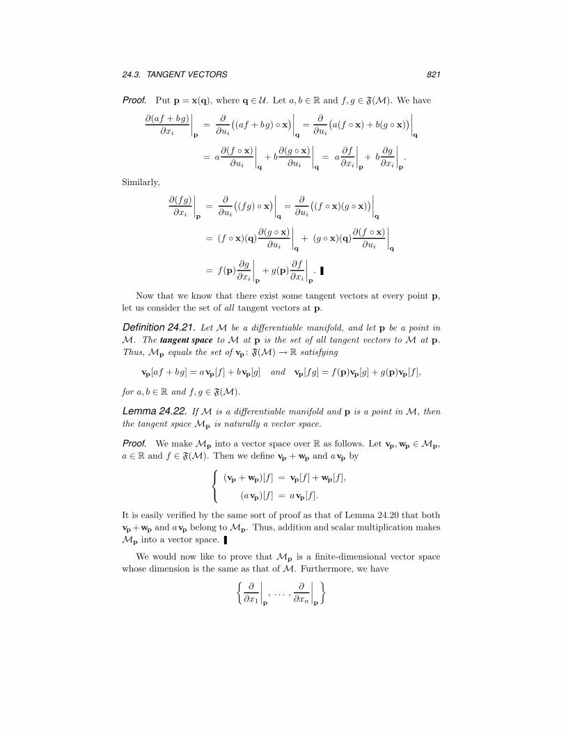
Proof. Put p = x(q), where q ∈ U . Let a, b ∈ R and f, g ∈ F(M). We have
∂(af + bg)
∂xi
∣∣∣∣p
=∂
∂ui
((af + bg) ◦ x
)∣∣∣∣q
=∂
∂ui
(a(f ◦ x) + b(g ◦ x)
)∣∣∣∣q
= a∂(f ◦ x)
∂ui
∣∣∣∣q
+ b∂(g ◦ x)
∂ui
∣∣∣∣q
= a∂f
∂xi
∣∣∣∣p
+ b∂g
∂xi
∣∣∣∣p
.
Similarly,
∂(fg)
∂xi
∣∣∣∣p
=∂
∂ui
((fg) ◦ x
)∣∣∣∣q
=∂
∂ui
((f ◦ x)(g ◦ x)
)∣∣∣∣q
= (f ◦ x)(q)∂(g ◦ x)
∂ui
∣∣∣∣q
+ (g ◦ x)(q)∂(f ◦ x)
∂ui
∣∣∣∣q
= f(p)∂g
∂xi
∣∣∣∣p
+ g(p)∂f
∂xi
∣∣∣∣p
.
Now that we know that there exist some tangent vectors at every point p,
let us consider the set of all tangent vectors at p.
Definition 24.21. Let M be a differentiable manifold, and let p be a point in
M. The tangent space to M at p is the set of all tangent vectors to M at p.
Thus, Mp equals the set of vp : F(M) → R satisfying
vp[af + bg] = avp[f ] + bvp[g] and vp[fg] = f(p)vp[g] + g(p)vp[f ],
for a, b ∈ R and f, g ∈ F(M).
Lemma 24.22. If M is a differentiable manifold and p is a point in M, then
the tangent space Mp is naturally a vector space.
Proof. We make Mp into a vector space over R as follows. Let vp,wp ∈ Mp,
a ∈ R and f ∈ F(M). Then we define vp + wp and avp by
(vp + wp)[f ] = vp[f ] + wp[f ],
(avp)[f ] = avp[f ].
It is easily verified by the same sort of proof as that of Lemma 24.20 that both
vp +wp and avp belong to Mp. Thus, addition and scalar multiplication makes
Mp into a vector space.
We would now like to prove that Mp is a finite-dimensional vector space
whose dimension is the same as that of M. Furthermore, we have{
∂
∂x1
∣∣∣∣p
, . . . ,∂
∂xn
∣∣∣∣p
}
822 CHAPTER 24. DIFFERENTIABLE MANIFOLDS
as a natural candidate for a basis of Mp. However, there are some technical
difficulties to overcome. First, we need
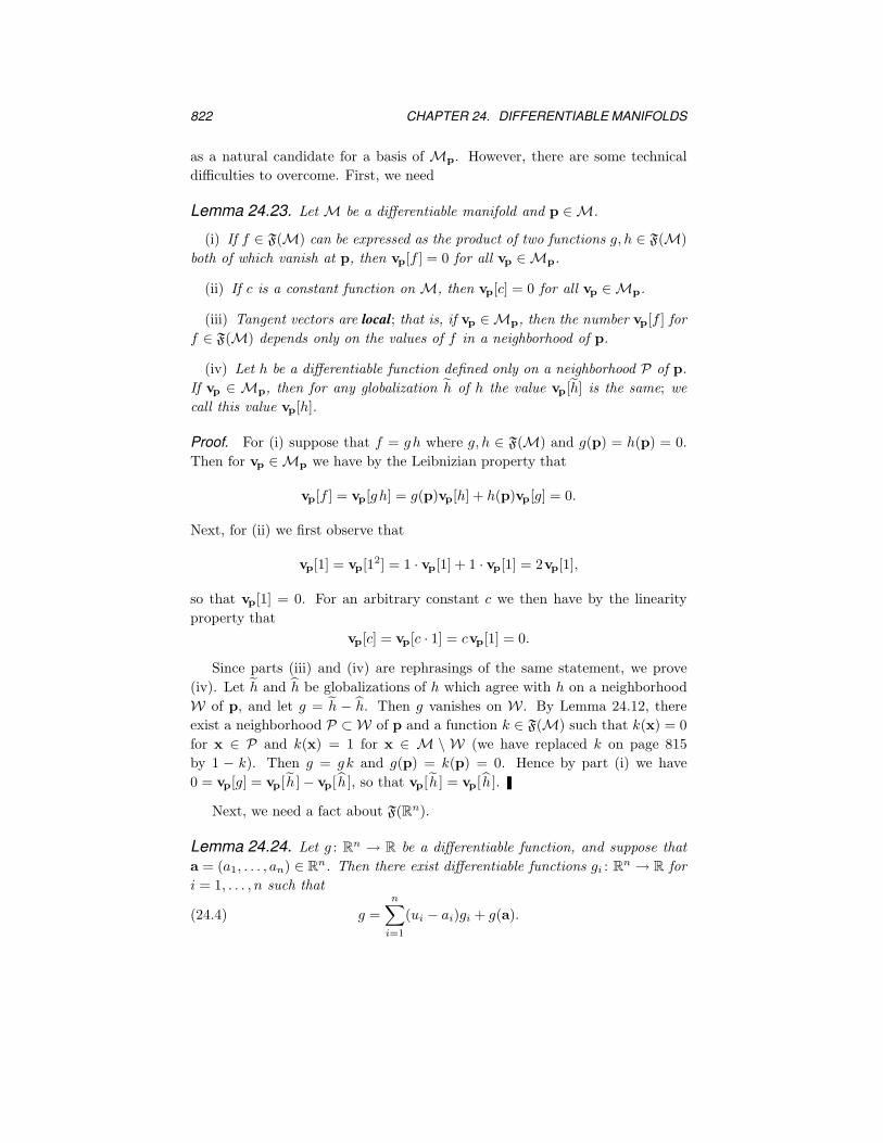
Lemma 24.23. Let M be a differentiable manifold and p ∈ M.
(i) If f ∈ F(M) can be expressed as the product of two functions g, h ∈ F(M)
both of which vanish at p, then vp[f ] = 0 for all vp ∈ Mp.
(ii) If c is a constant function on M, then vp[c] = 0 for all vp ∈ Mp.
(iii) Tangent vectors are local; that is, if vp ∈ Mp, then the number vp[f ] for
f ∈ F(M) depends only on the values of f in a neighborhood of p.
(iv) Let h be a differentiable function defined only on a neighborhood P of p.
If vp ∈ Mp, then for any globalization h of h the value vp[h] is the same; we
call this value vp[h].
Proof. For (i) suppose that f = gh where g, h ∈ F(M) and g(p) = h(p) = 0.
Then for vp ∈ Mp we have by the Leibnizian property that
vp[f ] = vp[gh] = g(p)vp[h] + h(p)vp[g] = 0.
Next, for (ii) we first observe that
vp[1] = vp[12] = 1 · vp[1] + 1 · vp[1] = 2vp[1],
so that vp[1] = 0. For an arbitrary constant c we then have by the linearity
property that
vp[c] = vp[c · 1] = cvp[1] = 0.
Since parts (iii) and (iv) are rephrasings of the same statement, we prove
(iv). Let h and h be globalizations of h which agree with h on a neighborhood
W of p, and let g = h − h. Then g vanishes on W . By Lemma 24.12, there
exist a neighborhood P ⊂ W of p and a function k ∈ F(M) such that k(x) = 0
for x ∈ P and k(x) = 1 for x ∈ M \ W (we have replaced k on page 815
by 1 − k). Then g = gk and g(p) = k(p) = 0. Hence by part (i) we have
0 = vp[g] = vp[ h ] − vp[ h ], so that vp[ h ] = vp[ h ].
Next, we need a fact about F(Rn).
Lemma 24.24. Let g : Rn → R be a differentiable function, and suppose that
a = (a1, . . . , an) ∈ Rn. Then there exist differentiable functions gi : R
n → R for
i = 1, . . . , n such that
g =
n∑
i=1
(ui − ai)gi + g(a).(24.4)

24.3. TANGENT VECTORS 823
Proof. Fix t = (t1, . . . , tn) ∈ Rn, and consider the function f : R → R defined
by
f(s) = g(st1 + (1 − s)a1, . . . , stn + (1 − s)an
)= g(st + (1 − s)a
).
Since g is differentiable, so is f , and
f ′(s) =
n∑
i=1
(ti − ai)∂g
∂ui
(st + (1 − s)a
).
Now ∫ 1
0
f ′(s)ds = f(1) − f(0) = g(t) − g(a),
and so the fundamental theorem of calculus implies that
g(t) − g(a) =
∫ 1
0
f ′(s)ds
=n∑
i=1
(ti − ai)
∫ 1
0
∂g
∂ui
(st + (1 − s)a
)ds
=n∑
i=1
(ui(t) − ai
)gi(t),
where
gi(t) =
∫ 1
0
∂g
∂ui
(st + (1 − s)a
)ds.
Clearly, the gi’s are differentiable. Thus we get (24.4).
Note that the proof of this lemma fails for Ck functions. If g is a Ck function,
we can only say that each gi is a Ck−1 function.
We are now able to prove:
Theorem 24.25. (Basis Theorem) Let x : U → M be a patch on a differentiable
manifold M with p ∈ x(U) and write x−1 = (x1, . . . , xn). If vp ∈ Mp, then
vp =
n∑
i=1
vp[xi]∂
∂xi
∣∣∣∣p
.
Proof. It suffices to show that
vp[f ] =
n∑
i=1
vp[xi]∂f
∂xi
∣∣∣∣∣p
(24.5)
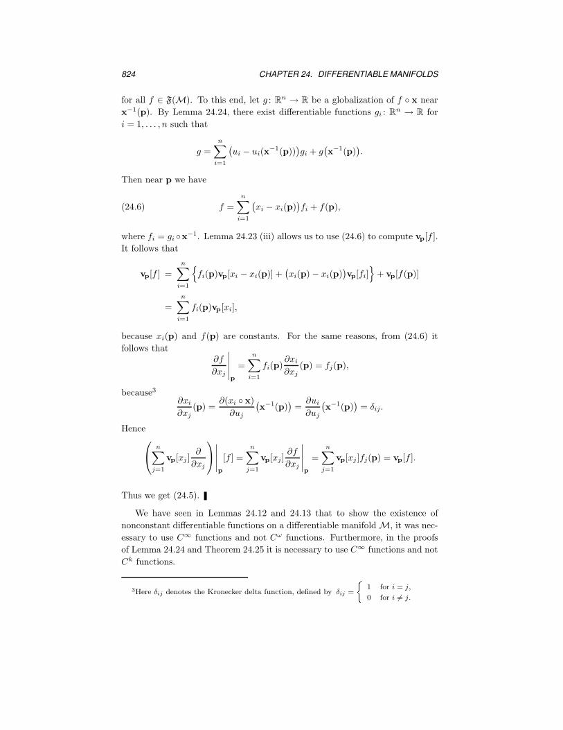
824 CHAPTER 24. DIFFERENTIABLE MANIFOLDS
for all f ∈ F(M). To this end, let g : Rn → R be a globalization of f ◦ x near
x−1(p). By Lemma 24.24, there exist differentiable functions gi : Rn → R for
i = 1, . . . , n such that
g =
n∑
i=1
(ui − ui(x
−1(p)))gi + g
(x−1(p)
).
Then near p we have
f =n∑
i=1
(xi − xi(p)
)fi + f(p),(24.6)
where fi = gi ◦x−1. Lemma 24.23 (iii) allows us to use (24.6) to compute vp[f ].
It follows that
vp[f ] =
n∑
i=1
{fi(p)vp[xi − xi(p)] +
(xi(p) − xi(p)
)vp[fi]
}+ vp[f(p)]
=
n∑
i=1
fi(p)vp[xi],
because xi(p) and f(p) are constants. For the same reasons, from (24.6) it
follows that∂f
∂xj
∣∣∣∣∣p
=
n∑
i=1
fi(p)∂xi
∂xj
(p) = fj(p),
because3
∂xi
∂xj
(p) =∂(xi ◦ x)
∂uj
(x−1(p)
)=∂ui
∂uj
(x−1(p)
)= δij .
Hence
n∑
j=1
vp[xj ]∂
∂xj
∣∣∣∣∣p
[f ] =
n∑
j=1
vp[xj ]∂f
∂xj
∣∣∣∣∣p
=
n∑
j=1
vp[xj ]fj(p) = vp[f ].
Thus we get (24.5).
We have seen in Lemmas 24.12 and 24.13 that to show the existence of
nonconstant differentiable functions on a differentiable manifold M, it was nec-
essary to use C∞ functions and not Cω functions. Furthermore, in the proofs
of Lemma 24.24 and Theorem 24.25 it is necessary to use C∞ functions and not
Ck functions.
3Here δij denotes the Kronecker delta function, defined by δij =
�1 for i = j,
0 for i 6= j.

24.3. TANGENT VECTORS 825
Corollary 24.26. Let x : U → M be a patch on a differentiable manifold M.
Let p ∈ x(U) and write x−1 = (x1, . . . , xn). Then the vectors
∂
∂x1
∣∣∣∣p
, . . . ,∂
∂xn
∣∣∣∣p
form a basis for the tangent space Mp. Hence the dimension of each tangent
space Mp as a vector space is the same as the dimension of M as a manifold.
Proof. The given vectors span the tangent space Mp by Theorem 24.25. To
prove they are linearly independent, suppose that a1, . . . , an ∈ R are such that
n∑
i=1
ai
∂
∂xi
∣∣∣∣p
= 0.
Then
0 =
n∑
i=1
ai
∂xj
∂xi
∣∣∣∣p
=
n∑
i=1
ai
∂(xj ◦ x)
∂ui
(x−1(p)
)=
n∑
i=1
aiδij = aj
for j = 1, . . . , n.
In order to differentiate functions on manifolds (that is, apply tangent vectors
to them) as easily as we would differentiate functions on Rn, we shall need the
following result that uses the same notation as Lemma 9.6 on page 267.
Lemma 24.27. (The Chain Rule) Let M be a differentiable manifold. Suppose
g1, . . . , gk ∈ F(M) and h ∈ F(Rk). Let f = h ◦ (g1, . . . , gk). Then for vp ∈ Mp
we have
vp[f ] =
k∑
i=1
∂h
∂ui
(g1(p), . . . , gk(p)
)vp[gi].(24.7)
Proof. Let g = (g1, . . . , gk). Define w : F(Rk) → R by
w[h] = vp[h ◦ g]
for h ∈ F(Rk). Then it is easy to check from the definition that w is an
element of the tangent space Rkg(p), because it is linear and Leibnizian. Using
Theorem 24.25 with the patch (u1, . . . , uk) at g(p) we get
w[h] =k∑
i=1
w[ui]∂h
∂ui
(g(p)
).(24.8)
Now w[h] = vp[h ◦ g] = vp[f ] and w[ui] = vp[ui ◦ g] = vp[gi], so that (24.8)
becomes
vp[f ] =
k∑
i=1
∂h
∂ui
(g(p)
)vp[gi].(24.9)
But (24.9) is another way of writing (24.7).

826 CHAPTER 24. DIFFERENTIABLE MANIFOLDS
Note that (24.7) allows us to transfer standard differentiation formulas from Rn
to manifolds. For example, if vp is a tangent vector to a manifold M at p and
f ∈ F(M), then vp[sin f ] = cos(f(p))vp[f ].
For abstract surface theory, it will be useful to have alternative notation for
tangent vectors.
Definition 24.28. Let x : U → M be a patch on a differentiable manifold M,
and let q ∈ U . Then
xui
(q): F(M) −→ R
is the operator given by
xui
(q)[f ] =∂(f ◦ x)
∂ui
∣∣∣∣q
(24.10)
for q ∈ U and f ∈ F(M).
The point is that (24.10) succeeds in generalizing the derivatives xu,xv defined
by (10.3) on page 289 to the more abstract setting of this chapter.
24.4 Induced Maps
In the previous section, we showed that to each point p of a differentiable
manifold M there is associated a vector space called the tangent space Mp. In
the present section we shall show how a differentiable map Ψ: M → N between
differentiable manifolds M and N gives rise to a linear map between tangent
spaces, in complete analogy to Definition 9.9 on page 268. Just as the tangent
space is the best linear approximation of a differentiable manifold, the tangent
map is the best linear approximation to a differentiable map between manifolds.
Definition 24.29. Let Ψ:M → N be a differentiable map between differentiable
manifolds M and N , and let p ∈ M. The tangent map of Ψ at p is the map
Ψ∗p
: Mp −→ NΨ(p)
given by
Ψ∗p
(vp)[f ] = vp[f ◦ Ψ](24.11)
for each f ∈ F(N ) and vp ∈ Mp.
In order for this definition to make sense, we must be sure that the image
of Ψ∗p is actually contained in the tangent space NΨ(p).
Lemma 24.30. Let Ψ: M → N be a differentiable map, and let p ∈ M,
vp ∈ Mp. Define
Ψ∗p(vp): F(N ) −→ R
by (24.11). Then Ψ∗p(vp) ∈ NΨ(p).
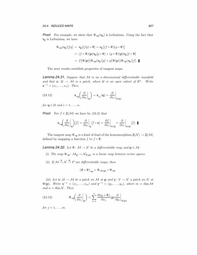
24.4. INDUCED MAPS 827
Proof. For example, we show that Ψ∗p(vp) is Leibnizian. Using the fact that
vp is Leibnizian, we have
Ψ∗p(vp)[fg] = vp[(fg) ◦ Ψ] = vp[(f ◦ Ψ)(g ◦ Ψ)
]
= (f ◦ Ψ)(p)vp[g ◦ Ψ] + (g ◦ Ψ)(p)vp[f ◦ Ψ]
= f(Ψ(p)
)Ψ∗p(vp)[g] + g
(Ψ(p)
)Ψ∗p(vp)[f ].
The next results establish properties of tangent maps.
Lemma 24.31. Suppose that M is an n-dimensional differentiable manifold
and that x : U → M is a patch, where U is an open subset of Rn. Write
x−1 = (x1, . . . , xn). Then
x∗q
(∂
∂ui
∣∣∣∣q
)= x
ui(q) =
∂
∂xi
∣∣∣∣x(q)
(24.12)
for q ∈ U and i = 1, . . . , n.
Proof. For f ∈ F(M) we have by (24.3) that
x∗q
(∂
∂ui
∣∣∣∣q
)[f ] =
∂
∂ui
∣∣∣∣q
[f ◦ x] =∂f
∂xi
∣∣∣∣x(q)
=∂
∂xi
∣∣∣∣x(q)
[f ].
The tangent map Ψ∗p is a kind of dual of the homomorphism F(N ) → F(M)
defined by mapping a function f to f ◦ Ψ.
Lemma 24.32. Let Ψ: M → N be a differentiable map and p ∈ M.
(i) The map Ψ∗p : Mp → NΨ(p) is a linear map between vector spaces.
(ii) If MΨ→ N
Φ→ P are differentiable maps, then
(Φ ◦ Ψ)∗p
= Φ∗Ψ(p) ◦ Ψ∗p.
(iii) Let x : U → M be a patch on M at p and y : V → N a patch on N at
Ψ(p). Write x−1 = (x1, . . . , xm) and y−1 = (y1, . . . , yn), where m = dimM
and n = dimN . Then
Ψ∗p
(∂
∂xj
∣∣∣∣p
)=
n∑
i=1
∂(yi ◦ Ψ)
∂xj
(p)∂
∂yi
∣∣∣∣Ψ(p)
(24.13)
for j = 1, . . . ,m.

828 CHAPTER 24. DIFFERENTIABLE MANIFOLDS
Proof. The proofs of (i) and (ii) are straightforward. To prove (iii), we use the
basis theorem (Theorem 24.25). Since
Ψ∗p
(∂
∂xj
∣∣∣∣p
)∈ NΨ(p),
and {∂
∂y1
∣∣∣∣Ψ(p)
, . . . ,∂
∂yn
∣∣∣∣Ψ(p)
}
is a basis for NΨ(p), we can write
Ψ∗p
(∂
∂xj
∣∣∣∣p
)=
n∑
i=1
aij
∂
∂yi
∣∣∣∣Ψ(p)
.(24.14)
To compute the aij ’s, we apply both sides of (24.14) to yk. We have
(n∑
i=1
aij
∂
∂yi
∣∣∣∣Ψ(p)
)[yk] = akj
while
Ψ∗p
(∂
∂xj
∣∣∣∣p
)[yk] =
(∂
∂xj
∣∣∣∣p
)[yk ◦ Ψ] =
∂(yk ◦ Ψ)
∂xj
(p).
Hence
aij =∂(yi ◦ Ψ)
∂xj
(p),
and we get (24.13).
Definition 24.33. Let Ψ: M → N be a differentiable map, where M, N are
differentiable manifolds of dimensions m,n respectively. Let p ∈ M, let (x,U)
be a patch on M at p and (y,V) a patch on N at Ψ(p). The Jacobian matrix
J(Ψ)(p) of Ψ at p relative to x and y is the matrix of Ψ∗p relative to the bases
{∂
∂x1
∣∣∣∣p
, . . . ,∂
∂xm
∣∣∣∣p
}and
{∂
∂y1
∣∣∣∣Ψ(p)
, . . . ,∂
∂yn
∣∣∣∣Ψ(p)
}.
Explicitly, J(Ψ)(p) is the matrix
(∂(yi ◦ Ψ)
∂xj
(p)
).
We can now get the manifold formulation of the inverse function theorem
from multivariable calculus:
Theorem 24.34. (Inverse Function Theorem) Let Ψ: M → N be a differen-
tiable map, and let p ∈ M. Suppose dimM = dimN = n. Then the following
conditions are equivalent:

24.4. INDUCED MAPS 829
(i) Ψ∗p is a linear isomorphism;
(ii) the Jacobian matrix J(Ψ)(p) is invertible;
(iii) there exist neighborhoods P of p and Q of Ψ(p) such that the restriction
Ψ |P : P → Q has a differentiable inverse (Ψ |P)−1 : Q → P.
Proof. That (i) implies (ii) is a standard fact of linear algebra. Also, it is easy
to see from Lemma 24.32(ii) that (iii) implies (i).
To show that (ii) implies (iii), consider y−1 ◦ Ψ ◦ x, where (x,U) is a patch
on M with p ∈ x(U) and (y,V) is a patch on N with Ψ(p) ∈ y(V). Without
loss of generality, we can assume that p = x(0) and Ψ(p) = y(0) so that
(y−1 ◦ Ψ ◦ x)(0) = 0.
Write x−1 = (x1, . . . , xn) and y−1 = (y1, . . . , yn). By assumption
det
(∂(ui ◦ y−1 ◦ Ψ ◦ x)
∂uj
(0)
)= det
(∂(yi ◦ Ψ)
∂xj
(p)
)= detJ(Ψ)(p) 6= 0.
The inverse function theorem for Rn implies that y−1 ◦Ψ◦x has a local inverse.
Hence so does Ψ.
Corollary 24.35. Let (x1, . . . , xn) be a coordinate system for M at p, where
each xj is defined on a neighborhood W of p. Then functions f1, . . . , fn ∈ F(W)
form a coordinate system for M at p if and only if
det
(∂fi
∂xj
)6= 0
on W.
Definition 24.36. A differentiable map Ψ: M → N is called regular, provided
Ψ∗p is a nonsingular linear transformation for each p ∈ M.
Corollary 24.37. A map Ψ: M → N is a local diffeomorphism if and only if
each Ψ∗p is a linear isomorphism.
Next, we discuss the notion of curve in a differentiable manifold using the
concepts we have developed. In what follows I denotes an open interval of the
real line R and d/du the natural coordinate vector field on it. For each t ∈ I we
have a canonical element of the tangent space Rt to R at the point t, namely
d
du
∣∣∣∣t
.

830 CHAPTER 24. DIFFERENTIABLE MANIFOLDS
Definition 24.38. A curve on a differentiable manifold M is a differentiable
function α : I → M. If t ∈ I the velocity vector of α at t is the tangent vector
α′(t) = α∗t
(d
du
∣∣∣∣t
)∈ M
α(t).
We do not exclude the possibility that the interval I is half-infinite or all
of R. One can usually arrange to have zero in the domain I of a curve α; it
is a convenient reference point. A curve on a surface in R3 is also a curve in
the sense of this definition and the two notions of velocity vector are equivalent.
We shall say that a curve α starts at p ∈ M provided that α(0) = p, and that
α has initial velocity vp ∈ Mp, provided α′(0) = vp. We leave the reader to
reconcile the notation α′(t) in Definition 24.38 with its usual meaning when α
is merely a differentiable mapping R → R.
Lemma 24.39. Let α : I → M be a curve. Then the value of the velocity vector
α′(t) on a function f ∈ F(M) is given by
α′(t)[f ] =d(f ◦ α)
du(t).
Proof. We have
α′(t)[f ] = α∗t
(d
du
∣∣∣∣t
)[f ] =
d(f ◦ α)
du(t).
Lemma 24.39 makes rigorous the earlier suggestion that for a tangent vector
vp the number vp[f ] is the derivative of f in the direction vp. This is because
for any curve α with initial velocity vp we have
vp[f ] =d(f ◦ α)
du(0).
Lemma 24.40. Let α be a curve in M, and let (x1, . . . , xn) be a coordinate
system at α(t) ∈ M. Then
α′(t) =
n∑
i=1
d(xi ◦ α)
du(t)
∂
∂xi
∣∣∣∣α(t)
.
Proof. This is an immediate consequence of Theorem 24.25.
A definition of the acceleration vector of a curve in an abstract manifold requires
a connection on the manifold, and is given in Section 25.1.
Next, we prove the generalization to differentiable manifolds of Lemma 1.9
on page 7. Although the following lemma can be proved by showing that it is a
special case of Lemma 24.27, it is easier to prove it directly.

24.5. VECTOR FIELDS 831
Lemma 24.41. (The Chain Rule for curves on a manifold) Let α : (a, b) → M
and h : (c, d) → (a, b) be differentiable. Put β = α ◦ h. Then
β′ = (α′ ◦ h)h′.
Proof. We have
β′(t) = β∗t
(d
du
∣∣∣∣t
)= α
∗h(t)◦ h
∗t
(d
du
∣∣∣∣t
)
= α∗h(t)
(h′(t)
d
du
∣∣∣∣h(t)
)= h′(t)α′
(h(t)
).
24.5 Vector Fields on Manifolds
The notion of derivation of an algebra comes up frequently in differential geom-
etry. Let us give the general definition and then specialize it to show that a
vector field is a derivation.
Definition 24.42. Let A be an algebra (which is not necessarily associative nor
commutative) over a field F. A derivation of A is a mapping D : A → A such
that {D(af + bg) = aDf + bDg,
D(fg) = f(Dg) + (Df)g
for all a, b ∈ F and f, g ∈ A.
Shortly, we shall define a vector field as a derivation of a special sort. But
first let us study derivations in general.
Definition 24.43. If D1 and D2 are derivations of an algebra, then the bracket
[D1, D2] of D1 and D2 is defined by
[D1, D2] = D1D2 −D2D1.
The proofs of the next two lemmas are easy.
Lemma 24.44. If D1 and D2 are derivations of an algebra, then so are [D1, D2],
D1 +D2 and aD1 for a ∈ F.
Lemma 24.45. Let D1, D2 and D3 be derivations of an algebra. Then:
(i) [D1, D2] = −[D2, D1].
(ii) The Jacobi identity holds:
[[D1, D2], D3
]+[[D3, D1], D2
]+[[D2, D3], D1
]= 0.
832 CHAPTER 24. DIFFERENTIABLE MANIFOLDS
We sometimes abbreviate the Jacobi identity to
S1,2,3
[[D1, D2], D3
]= 0,
where S denotes the cyclic sum. It is an important ingredient in
Definition 24.46. Let F be a field. A Lie algebra over F is a vector space V
over F with a bracket [ , ] : V × V → V such that
[X,X ] = 0,
[aX + bY, Z] = a[X,Z] + b[Y, Z],
[Z, aX + bY ] = a[Z,X ] + b[Z, Y ],
SX,Y,Z
[X, [Y, Z]
]= 0
for each X,Y, Z ∈ V and a, b ∈ F.
We have a ready-made example of a Lie algebra.
Lemma 24.47. Let A be a commutative algebra over a field F and denote by
D(A) the set of derivations of A. Then D(A) is a module over A and a Lie
algebra over F.
Derivations arise in many different contexts in differential geometry, and
the one of immediate interest provides us with an efficient way to extend the
definition of a vector field on Rn, given in Chapter 9, to manifolds.
Definition 24.48. A vector field X on a differentiable manifold M is a deriva-
tion of the algebra F(M) of real-valued differentiable functions on M.
Thus a vector field X on M is a mapping X : F(M) → F(M) satisfying
X[af + bg] = aX[f ] + bX[g] (the linearity property),
X[fg] = fX[g] + gX[f ] (the Leibnizian property),
for a, b ∈ R and f, g ∈ F(M). Also, the bracket [X,Y] of vector fields X and Y
is given by
[X,Y] = XY − YX.
Note that XY (defined by XY[f ] = X(Y[f ]) ) is a well-defined operator on
F(M), but not a vector field because the Leibnizian property is not satisfied.
We put
X(M) = {X | X is a vector field on M}.

24.5. VECTOR FIELDS 833
Lemma 24.47 tells us that X(M) is a module over F(M) and a Lie algebra
over R. In other words, we may multiply vector fields by either real numbers
or real-valued functions. Moreover, we have a bracket ‘multiplication’ between
vector fields that yields another vector field in X(M). The bracket is not mul-
tilinear with respect to functions; instead, there is a more complicated rule:
Lemma 24.49. Let X,Y ∈ X(M) and f, g ∈ F(M). Then
[fX, gY] = fg[X,Y] + fX[g]Y − gY[f ]X.(24.15)
The definition of vector field that we have given is very abstract. Probably
a more intuitive notion of vector field is that of a function that assigns to each
point p of a manifold M a tangent vector Xp. We now show that this intuitive
notion is equivalent to the definition that we have given. First, we introduce
Definition 24.50. The tangent bundle of a differentiable manifold M is the set
T (M) ={
(p,vp)∣∣ vp ∈ Mp, p ∈ M
}.
This object is both an important source of new manifolds, and a means of
interpreting the definition of vector field.
Theorem 24.51. The tangent bundle T (M) of a differentiable manifold M is
naturally a differentiable manifold whose dimension is twice the dimension of
M. Furthermore, the projection map π : T (M) → M defined by π(p,vp) = p is
a differentiable map.
Lemma 24.52. Associated with each vector field X ∈ X(M) is a section of
T (M), that is, a differentiable map X : M → T (M) such that π ◦ X = 1M,
where 1M denotes the identity map on M. In particular, X is a map that
associates a tangent vector Xp ∈ Mp with each point p ∈ M.
Conversely, each section of the tangent bundle gives rise in a natural way to
an element of X(M).
From now on we consider vector fields as derivations of F(M), or as sections
of T (M), whichever seems more convenient. If X ∈ X(M), we write Xp for the
tangent vector in Mp determined by X.
Definition 24.53. Let (x1, . . . , xn) be a system of local coordinates for M at p
defined on an open set W ⊂ M. Then
∂
∂xi
: F(W) −→ F(W)
is the operator that assigns to each function f ∈ F(W) its partial derivative
∂f/∂xi.
834 CHAPTER 24. DIFFERENTIABLE MANIFOLDS
The next lemma is an obvious consequence of Lemma 24.20.
Lemma 24.54. For each i = 1, . . . , n, and p ∈ W, we have
∂
∂xi
∈ X(W) and∂
∂xi
∣∣∣∣p
∈ Mp.
We are now in a position to give a version of the Basis Theorem on page 823
for vector fields.
Corollary 24.55. Let X ∈ X(M) and let x−1 = (x1, . . . , xn) be a system of
local coordinates defined on an open set W. Then X can be written as
X =
n∑
i=1
X[xi]∂
∂xi
(24.16)
on W.
Proof. It follows from Theorem 24.25 that
Xp =
n∑
i=1
Xp[xi]∂
∂xi
∣∣∣∣p
.(24.17)
Since (24.17) holds for all p ∈ W , we get (24.16).
We now consider the effect of a differentiable map Ψ: M → N on vector
fields. Unfortunately, it is not always possible to transfer vector fields on M to
vector fields on N . The problem is that if X ∈ X(M) and p,q ∈ M are points
such that Ψ(p) = Ψ(q), we may have that
Ψ∗p(Xp) 6= Ψ∗q(Xq).
An example of the phenomenon occurs for the vector field X in R3 defined by
X(x,y,z) = (−y, x, 0),
illustrated in Figure 24.3. The projection (x, y, z) 7→ (y, z) to the yz-plane
‘muddles up’ the vectors. By contrast, mapping (x, y, z) to (x, y) gives rise to
an unambiguous vector field in the xy-plane, and corresponds to the favorable
case formulated next.
Definition 24.56. Let Ψ: M → N be a differentiable map, and let X ∈ X(M),
Y ∈ X(N ). We say that X and Y are Ψrelated provided that
Ψ∗p
(Xp) = YΨ(p)
for all p ∈ M.
We use the notation XΨ = Y or Ψ∗(X) = Y, but beware that Y is not in
general determined by X if Ψ is not surjective.

24.5. VECTOR FIELDS 835
Figure 24.3: A swirling vector field in R3
The proof of the following results is straightforward.
Lemma 24.57. Let Ψ: M → N be a differentiable map.
(i) A vector field X ∈ X(M) is Ψ-related to a vector field Y ∈ X(N ) if and
only if
Y[f ] ◦ Ψ = X[f ◦ Ψ]
for all f ∈ F(N ).
(ii) Let W,X ∈ X(M) and Y,Z ∈ X(N ) with WΨ = Y and XΨ = Z. Then
[W,X] is Ψ-related to [Y,Z], so
[WΨ, XΨ] = [Y, Z] = [W, X]Ψ.
(iii) If Ψ: M → N is a diffeomorphism, then for any X ∈ X(M) there exists
a unique Y ∈ X(N ) such that XΨ = Y.
The vector-field version of Lemma 24.31 is
x∗
( ∂
∂ui
)=
∂
∂xi
= xui◦ x−1.(24.18)
From it, we may deduce an important vanishing result:

836 CHAPTER 24. DIFFERENTIABLE MANIFOLDS
Corollary 24.58. Let M be an n-dimensional differentiable manifold and let
x : U → M be a patch, where U is an open subset of Rn. Then
[∂
∂xi
,∂
∂xj
]=[x
ui, x
uj
]= 0,
for 1 6 i, j 6 n.
Proof. We have[∂
∂xi
,∂
∂xj
]=
[x∗
(∂
∂ui
), x∗
(∂
∂uj
)]= x∗
([∂
∂ui
,∂
∂uj
])= 0,
proving the second equation.
24.6 Tensor Fields
It will also be necessary to consider tensor fields. Tensor analysis was developed
by Ricci-Curbastro4 (see [Ricci]). The modern invariant notation described
below was introduced by Koszul [Kosz].
Instead of developing the most general situation, it will be sufficient for our
purposes to treat two special cases.
Definition 24.59. A covariant tensor field of degree r on a differentiable mani-
fold M is a mapping
α : X(M) × · · · × X(M)︸ ︷︷ ︸r times
−→ F(M)
that satisfies
α(X1, . . . , fiYi+giZi , . . . , Xr) = fiα(X1, . . . ,Yi, . . . , Xr)(24.19)
+ giα(X1, . . . ,Zi, . . . , Xr)
for all fi, gi ∈ F(M), X1, . . . ,Xr, Yi,Zi ∈ X(M), and for each index i in turn.
A vectorvariant tensor field of degree r is a mapping
Φ: X(M) × · · · × X(M)︸ ︷︷ ︸r times
−→ X(M)
that satisfies (24.19).
4
Gregorio Ricci-Curbastro (1853–1925). Italian mathematician, professor
at the University of Padua. He invented the absolute differential calculus
between 1884 and 1894. It became the foundation of the tensor analysis
that was used by Einstein in his theory of general relativity (see [HaEl]).
24.6. TENSOR FIELDS 837
Remarks
(1) Condition (24.19) asserts that α and Φ are multilinear with respect to
functions. On the other hand, the Lie bracket [ , ] is not a tensor field
because it is not multilinear with respect to functions; instead it satisfies
the more complicated formula (24.15).
(2) Sometimes a covariant tensor field of degree r is said to be a tensor field
of type (r, 0), and a vectorvariant tensor field of degree r is said to be a
tensor field of type (r, 1). It is also possible to define tensor fields of type
(r, s), but we ignore the case s > 2.
(3) There is actually a definition in linear algebra that is very similar to the
definition of tensor field. Applying it to the tangent space at a point p to
a differentiable manifold M gives
Definition 24.60. A covariant tensor at p ∈ M is a multilinear map
α : Mp × · · · ×Mp︸ ︷︷ ︸r times
−→ R
that satisfies
α(x1, . . . , aiyi+bizi, . . . , xr) = aiα(x1, . . . ,yi, . . . , xr)
+ biα(x1, . . . ,zi, . . . , xr)
for all ai, bi ∈ R, and all x1, . . . ,xr, yi, zi ∈ Mp. A vectorvariant tensor
at x is defined similarly, by replacing R with Mp.
On page 834 we noted that some differentiable mappings between manifolds
M and N do not always induce a map between the algebras of vector fields of
M and N . The situation is much better with covariant tensor fields.
Definition 24.61. Let Ψ: M → N be a differentiable mapping, and let α be a
covariant tensor field of degree r on N . Then the pullback of α is the covariant
tensor field Ψ∗(α) on M given by
Ψ∗(α)(v1, . . . ,vr) = α(Ψ∗p(v1), . . . , Ψ∗p(vr)
),
where v1, . . . ,vr are arbitrary tangent vectors at an arbitrary point p ∈ M.
The following lemma is easy to prove.
Lemma 24.62. Let Ψ: M → N be a differentiable mapping, and let α and β
be covariant tensor fields of degree r on N . Also, let f, g ∈ F(N ). Then
Ψ∗(fα+ gβ) = (f ◦ Ψ)Ψ∗(α) + (g ◦ Ψ)Ψ∗(β).

838 CHAPTER 24. DIFFERENTIABLE MANIFOLDS
Let us single out one of the simplest types of covariant tensor fields.
Definition 24.63. A differential 1form on a manifold M is an F(M)-linear
map
ω : X(M) −→ F(M).
In other words, a 1-form ω has the property that
ω(fX + gY) = f ω(X) + gω(Y)
for f, g ∈ F(M) and X,Y ∈ X(M). We denote the collection of 1-forms on M
by X(M)∗, and we make it into a module over F(M) by defining
(f ω + gθ)(X) = f ω(X) + gθ(X)
for f, g ∈ F(M), ω, θ ∈ X(M)∗ and X ∈ X(M).
If V is any vector space over any field F (in our case, almost invariably R),
its dual space is denoted by V ∗. It is the new vector space
V ∗ = { α : V → F | α is linear }
consisting of linear functionals, or linear mappings from V to the field. We see
that Definition 24.63 extends this concept to modules, so that X(M)∗ is the
dual module of X(M).
Lemma 24.64. Suppose X ∈ X(M) and p ∈ M are such that Xp = 0. Then
ω(X)(p) = 0
for all ω ∈ X(M)∗.
Proof. Let (x,U) be a patch on M at p with x−1 = (x1, . . . , xn). Using
Corollary 24.55, we have
X =
n∑
i=1
X[xi]∂
∂xi
near p. Also, Xp = 0 implies that X[xi](p) = 0 for i = 1, . . . , n. Hence,
ω(X)(p) = ω
(n∑
i=1
X[xi]∂
∂xi
)(p) =
n∑
i=1
X[xi](p) ω
(∂
∂xi
)(p) = 0.
We can evaluate 1-forms at a point in the same way that we evaluate vector
fields at a point.
Definition 24.65. Let ω ∈ X(M)∗ and p ∈ M. Then ωp : Mp → R is defined
by
ωp(v) = ω(X)(p),
where X ∈ X(M) is any vector field for which Xp = v.
24.7. EXERCISES 839
Lemma 24.66. The definition of ωp does not depend on the choice of the vector
field X.
Proof. Let X and X be vector fields such that Xp = Xp = v. Then X − X
vanishes at p so by Lemma 24.64,
ω(X)(p) − ω(X)(p) = ω(X − X)(p) = 0.
There is a particularly important kind of 1-form.
Definition 24.67. For f ∈ F(M) the differential df of f is the 1-form defined
by
df(X) = X[f ]
for X ∈ X(M).
We conclude this chapter with
Lemma 24.68. Let (x1, . . . , xn) be a system of coordinates defined on an open
set W ⊂ M. Then
(i) For each p ∈ W, the 1-forms dx1(p), . . . , dxn(p) form a basis of M∗p.
Hence
{ ωp | ω ∈ X(M)∗ } = M∗p.
(ii) The set {dx1, . . . , dxn} is a basis for X(W)∗. Thus for any ω ∈ X(W)∗,
we can write
ω =
n∑
i=1
ω
(∂
∂xi
)dxi.
24.7 Exercises
1. If M1 and M2 are differentiable manifolds, show that M1 × M2 is a
differentiable manifold.
2. Show that each tangent space Mp to a differentiable manifold M is itself
a differentiable manifold.
3. Let Φ: R → R be defined by Φ(t) = t3. Show that the complete atlas A2
on R containing the patch (Φ,R) is different from the usual complete atlas
A1 containing the identity patch (1,R). Show that (R, A1) and (R, A2)
are nonetheless diffeomorphic.
840 CHAPTER 24. DIFFERENTIABLE MANIFOLDS
4. Recall the definition of real projective space RPn in Exercise 12 of the
previous chapter, and define again p : Sn(1) 7→ RPn by p(a) = {a,−a}.
Let
Pj = { p(a1, . . . , an) | aj 6= 0}.
Show that:
(a) Each Pj is an open subset of RPn.
(b) RPn is the union of all the Pj’s.
(c) For each j, there is a homeomorphism ψj : Pj → Rn.
(d) RPn is a compact differentiable manifold of dimension n.
5. On R3 consider the vector fields
X = x2 ∂
∂x+ y
∂
∂zand Y = y3 ∂
∂y,
and the function f : R3 → R defined by f(p1, p2, p3) = p12p2p3. Compute
(a) [X,Y](1,0,1)
(b) (fY)(1,0,1)
(c) (Yf)(1, 0, 1)
(d) f∗(1,0,1)
(Y
(1,0,1)
).
Give examples of vector fields X and Y on R2 for which
X(0,0)
= Y(0,0)
but [X,Y](0,0)
6= 0.
6. Let Φ: R3 → R2 be defined by Φ(p1, p2, p3) = (p1, p2), and let Z be the
vector field on R3 given by
Z = cos z∂
∂x+ sin z
∂
∂y+
∂
∂z,
where x, y, z are the natural coordinate functions of R3. Show that there
is no vector field Y on R2 for which
Φ∗p
(Z) = YΦ(p)
for all p ∈ R3.
7. Set W = {(u, v) ∈ R2 | uv > 0}. Let f : R
2 → R2 and g : W → R
3 be
defined by
f(u, v) = (u2 sin v, euv) and g(u, v) = (uv2, log(uv), v sinu).
Compute the matrices of f∗ and g∗ with respect to the standard bases of
vector fields on R2 and R3.

24.7. EXERCISES 841
8. Prove Lemma 24.62.
9. Define, for each patch (x,U) on an n-dimensional differentiable manifold
M, an associated patch x : U ×Rn → T (M) on the tangent bundle of M
by setting
x(p,q) =
(x(p), x
∗p
( n∑
i=1
qi∂
∂ui
)),
where p ∈ U and q = (q1, . . . , qn). Show that the tangent bundle T (M)
becomes a differentiable manifold with atlas
{(x, U × R
n)∣∣ (x,U) is a patch on M
}.
10. Define, for fixed a > 0, a mapping from an open set of Rn+1 to R
n by
stereo(q0, q1, . . . , qn) =a
a− q0(q1, . . . , qn).(24.20)
Referring to page 813, show that the composition stereo ◦ north equals
the identity map from Rn to itself. Observe that (24.20) generalizes the
mapping of the same name on page 730 to the case of arbitary n and a.