difference in difference models part2.pptxwevans1/econ30331/difference in difference models... ·...

11/12/2012

1

11

Difference in Difference –Part 2

Bill Evans

2

Making the model more complicated

• So far, a very simple model– Two groups– Two periods

• However, the “treatment” may cover more than 1 group

• The treatment may happen at very different time periods across groups

• How to generalize this type of model for– Many treatments– Multiple groups being treated

3

Example: States as laboratories

• Tremendous variation across states in their laws– Variation across states in any given year

– Variation over time within a state

• Examples– Minimum wages, welfare policy, Medicaid

coverage, traffic safety laws, use of death penalty, drinking age, cigarette taxes,

4

Empirical example: Motorcycle Helmet laws

• 1967, Feds require states to have helmet law to get all federal highway money

• By 1975, all states have qualifying law

• 1976, Congress responds to state pressure and eliminate penalties– 20 states weaken their law and only require

coverage for teens

– 8 states repeal law completely

11/12/2012

2

5

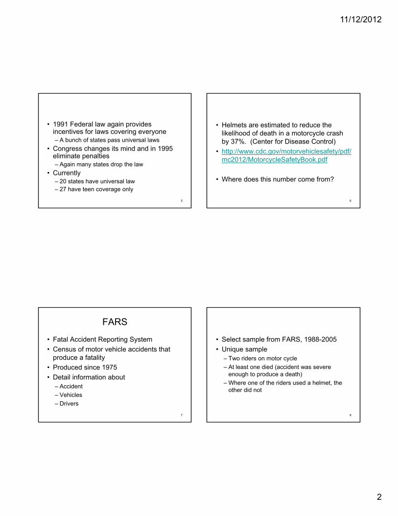
• 1991 Federal law again provides incentives for laws covering everyone– A bunch of states pass universal laws

• Congress changes its mind and in 1995 eliminate penalties– Again many states drop the law

• Currently– 20 states have universal law– 27 have teen coverage only

• Helmets are estimated to reduce the likelihood of death in a motorcycle crash by 37%. (Center for Disease Control)

• http://www.cdc.gov/motorvehiclesafety/pdf/mc2012/MotorcycleSafetyBook.pdf

• Where does this number come from?

6

FARS

• Fatal Accident Reporting System

• Census of motor vehicle accidents that produce a fatality

• Produced since 1975

• Detail information about– Accident

– Vehicles

– Drivers

7

• Select sample from FARS, 1988-2005

• Unique sample– Two riders on motor cycle

– At least one died (accident was severe enough to produce a death)

– Where one of the riders used a helmet, the other did not

8

11/12/2012

3

9

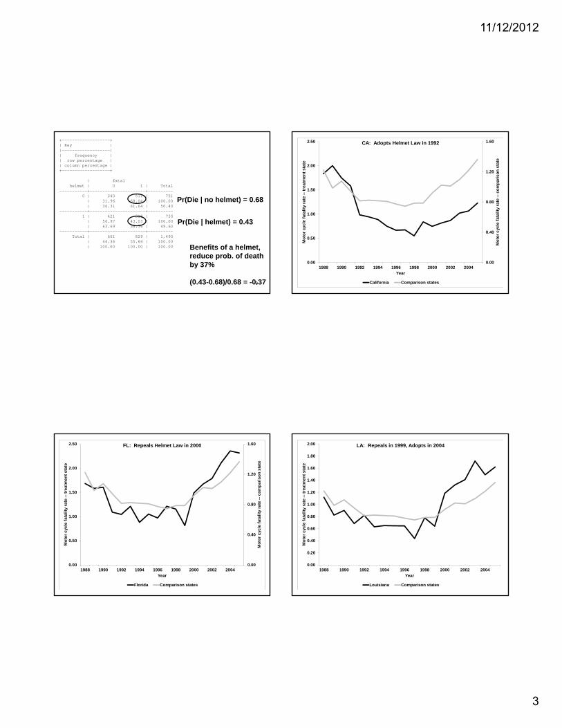
+-------------------+| Key ||-------------------|| frequency || row percentage || column percentage |+-------------------+

| fatalhelmet | 0 1 | Total

-----------+----------------------+----------0 | 240 511 | 751 | 31.96 68.04 | 100.00 | 36.31 61.64 | 50.40

-----------+----------------------+----------1 | 421 318 | 739 | 56.97 43.03 | 100.00 | 63.69 38.36 | 49.60

-----------+----------------------+----------Total | 661 829 | 1,490

| 44.36 55.64 | 100.00 | 100.00 100.00 | 100.00

Pr(Die | no helmet) = 0.68

Pr(Die | helmet) = 0.43

Benefits of a helmet,reduce prob. of deathby 37%

(0.43-0.68)/0.68 = -0.37 10

0.00

0.40

0.80

1.20

1.60

0.00

0.50

1.00

1.50

2.00

2.50

1988 1990 1992 1994 1996 1998 2000 2002 2004

Mo

tor

cyc

le f

ata

lity

ra

te -

-co

mp

aris

on

sta

te

Mo

tor

cyc

le f

ata

lity

rat

e --

tre

atm

en

t s

tate

Year

CA: Adopts Helmet Law in 1992

California Comparison states

11

0.00

0.40

0.80

1.20

1.60

0.00

0.50

1.00

1.50

2.00

2.50

1988 1990 1992 1994 1996 1998 2000 2002 2004

Mo

tor

cyc

le f

ata

lity

ra

te -

-co

mp

aris

on

sta

te

Mo

tor

cyc

le f

ata

lity

rat

e --

tre

atm

en

t s

tate

Year

FL: Repeals Helmet Law in 2000

Florida Comparison states 12

0.00

0.20

0.40

0.60

0.80

1.00

1.20

1.40

1.60

1.80

2.00

1988 1990 1992 1994 1996 1998 2000 2002 2004

Mo

tor

cyc

le f

ata

lity

rat

e --

tre

atm

en

t s

tate

Year

LA: Repeals in 1999, Adopts in 2004

Louisiana Comparison states

11/12/2012

4

13

0.00

0.20

0.40

0.60

0.80

1.00

1.20

1.40

1.60

1.80

2.00

1988 1990 1992 1994 1996 1998 2000 2002 2004

Mo

tor

cyc

le f

ata

lity

rat

e --

tre

atm

en

t s

tate

Year

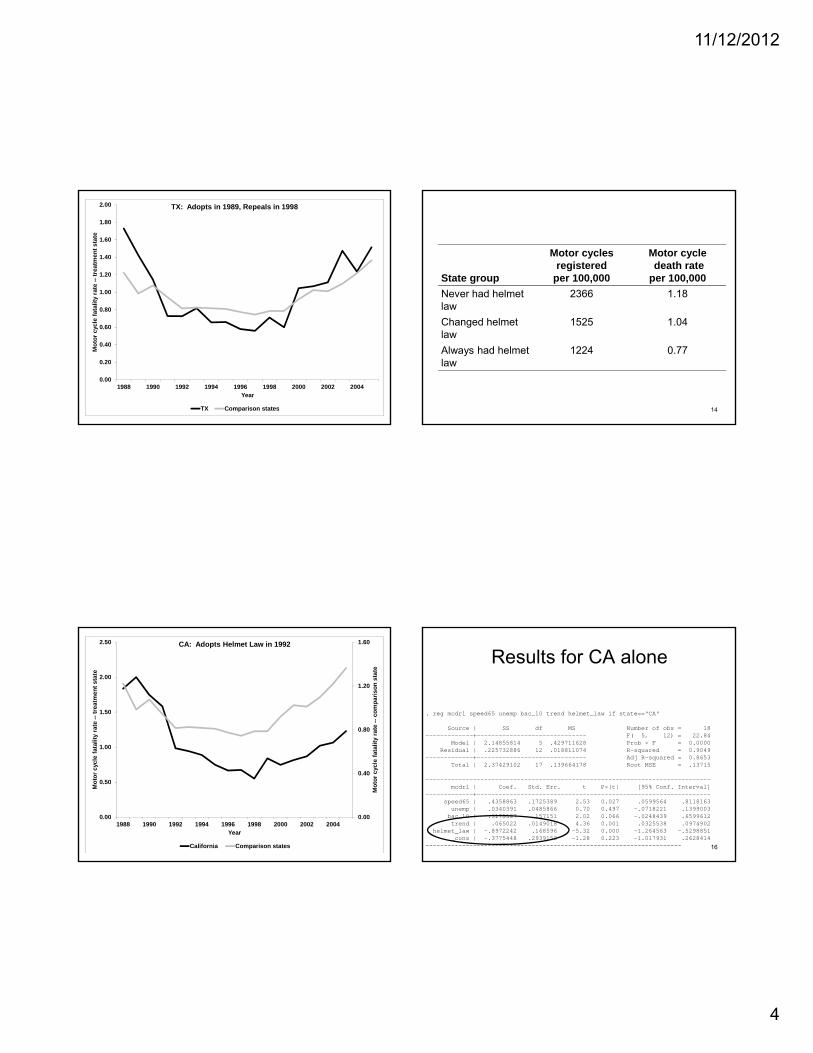
TX: Adopts in 1989, Repeals in 1998

TX Comparison states

State group

Motor cycles registered

per 100,000

Motor cycledeath rate

per 100,000

Never had helmet law

2366 1.18

Changed helmet law

1525 1.04

Always had helmet law

1224 0.77

14

15

0.00

0.40

0.80

1.20

1.60

0.00

0.50

1.00

1.50

2.00

2.50

1988 1990 1992 1994 1996 1998 2000 2002 2004

Mo

tor

cyc

le f

ata

lity

ra

te -

-co

mp

aris

on

sta

te

Mo

tor

cyc

le f

ata

lity

rat

e --

tre

atm

en

t s

tate

Year

CA: Adopts Helmet Law in 1992

California Comparison states

Results for CA alone

16

. reg mcdrl speed65 unemp bac_10 trend helmet_law if state=="CA"

Source | SS df MS Number of obs = 18-------------+------------------------------ F( 5, 12) = 22.84

Model | 2.14855814 5 .429711628 Prob > F = 0.0000Residual | .225732886 12 .018811074 R-squared = 0.9049

-------------+------------------------------ Adj R-squared = 0.8653Total | 2.37429102 17 .139664178 Root MSE = .13715

------------------------------------------------------------------------------mcdrl | Coef. Std. Err. t P>|t| [95% Conf. Interval]

-------------+----------------------------------------------------------------speed65 | .4358863 .1725389 2.53 0.027 .0599564 .8118163unemp | .0340391 .0485866 0.70 0.497 -.0718221 .1399003bac_10 | .3175587 .157151 2.02 0.066 -.0248439 .6599612trend | .065022 .0149018 4.36 0.001 .0325538 .0974902

helmet_law | -.8972242 .168596 -5.32 0.000 -1.264563 -.5298851_cons | -.3775448 .2939152 -1.28 0.223 -1.017931 .2628414

----------------------------------------------------------------------

11/12/2012

5

17

0.00

0.20

0.40

0.60

0.80

1.00

1.20

1.40

1.60

1.80

2.00

1988 1990 1992 1994 1996 1998 2000 2002 2004

Mo

tor

cyc

le f

ata

lity

rat

e --

tre

atm

en

t s

tate

Year

TX: Adopts in 1989, Repeals in 1998

TX Comparison states

Results for TX alone

18

* run a model for Texas. reg mcdrl speed65 unemp bac_08 trend helmet_law if state=="TX"


Model | 1.86115335 5 .37223067 Prob > F = 0.0008Residual | .473677129 12 .039473094 R-squared = 0.7971



-------------+----------------------------------------------------------------speed65 | .1689669 .2624034 0.64 0.532 -.4027609 .7406947unemp | .1301635 .0747096 1.74 0.107 -.0326147 .2929418bac_08 | .6692796 .2457196 2.72 0.018 .1339026 1.204657trend | -.0405022 .0284775 -1.42 0.180 -.1025494 .021545

helmet_law | -.4592142 .1645968 -2.79 0.016 -.8178398 -.1005887_cons | -.5765997 .464616 -1.24 0.238 -1.588911 .4357116

-----------------------------------------------------------------------

Purely Cross Sectional Model (1990)

19

. * run basic OLS model for 1990

. reg mcdrl speed65 unemp bac_08 bac_10 helmet_law if year==1990


Model | 2.59400681 5 .518801363 Prob > F = 0.0023Residual | 4.86098775 42 .115737804 R-squared = 0.3480



-------------+----------------------------------------------------------------speed65 | .1692481 .1357937 1.25 0.220 -.1047947 .4432909unemp | .0524134 .0490639 1.07 0.292 -.0466015 .1514283bac_08 | -.0944842 .2372792 -0.40 0.693 -.573333 .3843645bac_10 | .01337 94.1658892 0.08 0.936 -.3213985 .3481573

helmet_law | -.4684841 .1038582 -4.51 0.000 -.6780784 -.2588898_cons | -.0643492 .3042114 -0.21 0.833 -.6782726 .5495743

------------------------------------------------------------------------------20

0 1 2

2 2

:

1,2,... ; 1, 2,...

1 , 0

1 , 0

1

, 0

i

t

it

it it i

n T

j j k k itj k

define

i n t T

S if state i otherwise

W if year t otherwise

Law if state i has helmet law

in year t otherwise

y REFORM x

S W

11/12/2012

6

21

• Why k=2 to N and j=2 to T?

• What does α measure?

• What does λ measure?

22

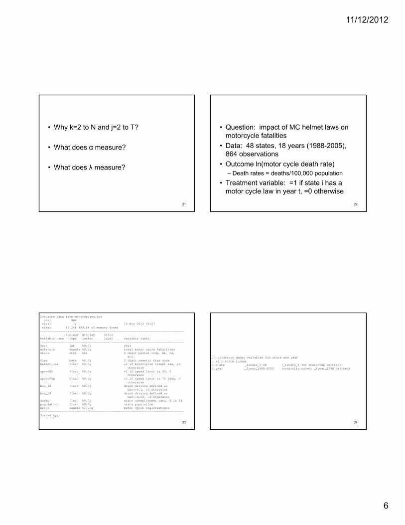
• Question: impact of MC helmet laws on motorcycle fatalities

• Data: 48 states, 18 years (1988-2005), 864 observations

• Outcome ln(motor cycle death rate)– Death rates = deaths/100,000 population

• Treatment variable: =1 if state i has a motor cycle law in year t, =0 otherwise

23

Contains data from motorcycles.dtaobs: 864 vars: 12 10 Nov 2012 09:27size: 49,248 (99.6% of memory free)-------------------------------------------------------------------------------

storage display valuevariable name type format label variable label-------------------------------------------------------------------------------year int %9.0g yearmcfatals double %9.0g total motor cycle fatalitiesstate str2 %2s 2 digit postal code, AL, CA,

etc.fips byte %8.0g 2 digit numeric fips codehelmet_law float %9.0g =1 if motorcycle helmet law, =0

otherwisespeed65 float %9.0g =1 if speed limit is 65, 0

otherwisespeed70p float %9.0g =1 if speed limit is 70 plus, 0

otherwisebac_10 float %9.0g drunk driving defined as

bac>=0.1, =0 otherwisebac_08 float %9.0g drunk driving defined as

bac>=0.08, =0 otherwiseunemp float %9.0g state unemployment rate, 5 is 5%population float %9.0g state populationmregs double %10.0g motor cycle registrations-------------------------------------------------------------------------------Sorted by:

24

. * construct dummy variables for state and year

. xi i.state i.yeari.state _Istate_1-48 (_Istate_1 for state==AL omitted)i.year _Iyear_1988-2005 (naturally coded; _Iyear_1988 omitted)

11/12/2012

7

25

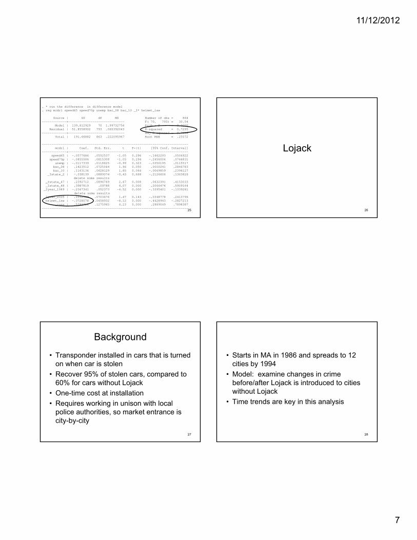
. * run the difference in difference model

. reg mcdrl speed65 speed70p unemp bac_08 bac_10 _I* helmet_law


Model | 139.812929 70 1.99732756 Prob > F = 0.0000Residual | 51.8558902 793 .065392043 R-squared = 0.7295



-------------+----------------------------------------------------------------speed65 | -.0577686 .0552537 -1.05 0.296 -.1662293 .0506922speed70p | -.0855586 .0815308 -1.05 0.294 -.2456004 .0744831

unemp | -.0117339 .0118625 -0.99 0.323 -.0350195 .0115517bac_08 | .1423512 .0725064 1.96 0.050 .0000241 .2846783bac_10 | .1163134 .0628129 1.85 0.064 -.0069859 .2396127

_Istate_2 | -.038139 .0889074 -0.43 0.668 -.2126606 .1363826delete some results

_Istate_47 | .2392712 .0896769 2.67 0.008 .0632391 .4153033_Istate_48 | .3987819 .09788 4.07 0.000 .2066474 .5909164_Iyear_1989 | -.2367341 .052373 -4.52 0.000 -.3395401 -.1339281

delete some results_Iyear_2005 | .1032509 .0703676 1.47 0.143 -.0348778 .2413796helmet_law | -.3728078 .0458932 -8.12 0.000 -.4628943 -.2827213

_cons | .5393718 .1275965 4.23 0.000 .2889049 .7898387------------------------------------------------------------------------------

Lojack

26

Background

• Transponder installed in cars that is turned on when car is stolen

• Recover 95% of stolen cars, compared to 60% for cars without Lojack

• One-time cost at installation

• Requires working in unison with local police authorities, so market entrance is city-by-city

27

• Starts in MA in 1986 and spreads to 12 cities by 1994

• Model: examine changes in crime before/after Lojack is introduced to cities without Lojack

• Time trends are key in this analysis

28

11/12/2012

8

29 30

31 32

11/12/2012

9

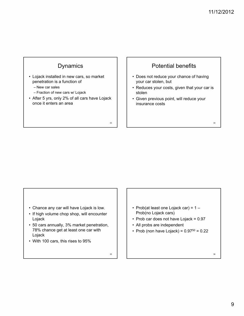
Dynamics

• Lojack installed in new cars, so market penetration is a function of– New car sales

– Fraction of new cars w/ Lojack

• After 5 yrs, only 2% of all cars have Lojack once it enters an area

33

Potential benefits

• Does not reduce your chance of having your car stolen, but

• Reduces your costs, given that your car is stolen

• Given previous point, will reduce your insurance costs

34

• Chance any car will have Lojack is low.

• If high volume chop shop, will encounter Lojack

• 50 cars annually, 3% market penetration, 78% chance get at least one car with Lojack

• With 100 cars, this rises to 95%

35

• Prob(at least one Lojack car) = 1 –Prob(no Lojack cars)

• Prob car does not have Lojack = 0.97

• All probs are independent

• Prob (non have Lojack) = 0.9750 = 0.22

36

11/12/2012

10

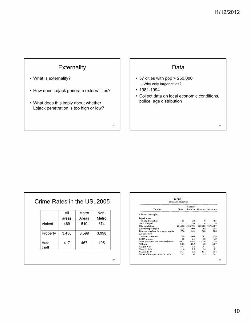
Externality

• What is externality?

• How does Lojack generate externalities?

• What does this imply about whether Lojack penetration is too high or low?

37

Data

• 57 cities with pop > 250,000– Why only larger cities?

• 1981-1994

• Collect data on local economic conditions, police, age distribution

38

Crime Rates in the US, 2005

All

areas

Metro

Areas

Non-

Metro

Violent 469 510 374

Property 3,430 3,599 3,998

Auto theft

417 467 195

39 40

11/12/2012

11

41

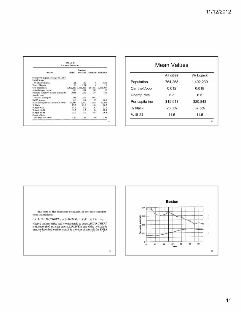
Mean Values

All cities W/ Lojack

Population 764,268 1,402,239

Car theft/pop 0.012 0.018

Unemp rate 6.3 6.5

Per capita inc $19,911 $20,843

% black 26.0% 37.5%

%18-24 11.5 11.5

42

43 44

11/12/2012

12

45 46

47 48

11/12/2012

13

49

Linden and Rockoff

• Megan Kanka– 7 year old girl

– Raped and murdered by neighbor who was convicted sex offender

• No one in the neighborhood knew about neighbor’s history

• Lead to passage of “Megan’s Law”

50

Megan’s Law

• Sexual Offender (Jacob Wetterling) Act of 1994– Sexual offenders required to notify state of

change of address

– Time limits vary across states (10 years after conviction or life)

– Required of all child sex offenders, some states require of all offenders

51

Megan’s Law

• 1996 Amendment to original law required states to publicly announce location and type of offense of sex offenders

• Indiana site

• http://www.icrimewatch.net/indiana.php

52

11/12/2012

14

Economic question

• Crime negatively impacts property values• Problem: crime is not random and neither

are home purchases• Therefore, getting an estimate of the

impact of crime on housing prices is tough• Megan’s law

– Sex offenders will most likely live in poorer areas

– How to separate thus fact from their impact on house prices?

53

Methodology

• Compare house sales in neighborhoods before and after arrival of sex offender

• Impact should be “local” so comparison sample included homes in the same neighborhood but not near the offender

54

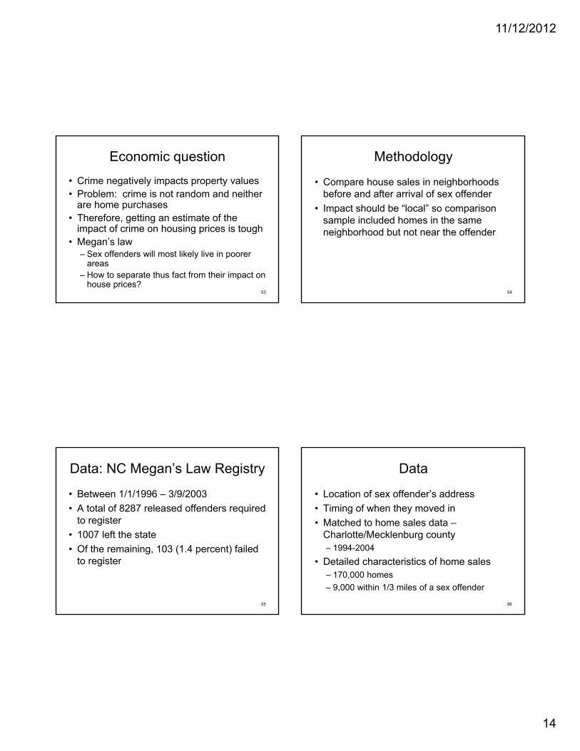
Data: NC Megan’s Law Registry

• Between 1/1/1996 – 3/9/2003

• A total of 8287 released offenders required to register

• 1007 left the state

• Of the remaining, 103 (1.4 percent) failed to register

55

Data

• Location of sex offender’s address

• Timing of when they moved in

• Matched to home sales data –Charlotte/Mecklenburg county– 1994-2004

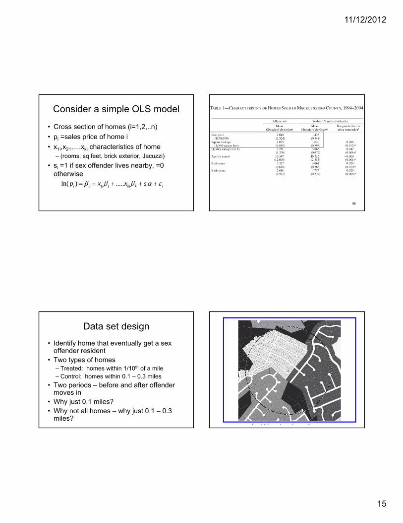
• Detailed characteristics of home sales– 170,000 homes

– 9,000 within 1/3 miles of a sex offender

56

11/12/2012

15

Consider a simple OLS model

• Cross section of homes (i=1,2,..n)

• pi =sales price of home i

• x1i,x21,....xki characteristics of home– (rooms, sq feet, brick exterior, Jacuzzi)

• si =1 if sex offender lives nearby, =0 otherwise

0 1 1ln( ) .....i i ki k i ip x x s

58

Data set design

• Identify home that eventually get a sex offender resident

• Two types of homes– Treated: homes within 1/10th of a mile– Control: homes within 0.1 – 0.3 miles

• Two periods – before and after offender moves in

• Why just 0.1 miles?• Why not all homes – why just 0.1 – 0.3

miles? 60

11/12/2012

16

61

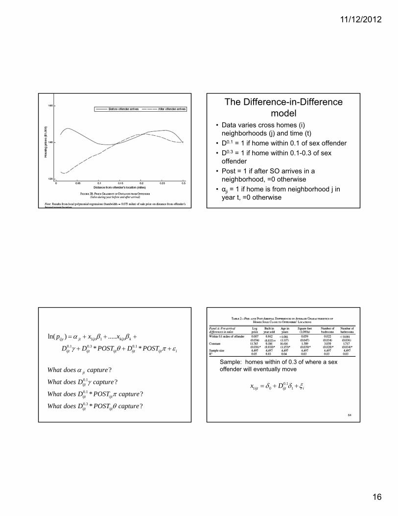
The Difference-in-Difference model

• Data varies cross homes (i) neighborhoods (j) and time (t)

• D0.1 = 1 if home within 0.1 of sex offender

• D0.3 = 1 if home within 0.1-0.3 of sex offender

• Post = 1 if after SO arrives in a neighborhood, =0 otherwise

• αji = 1 if home is from neighborhood j in year t, =0 otherwise

1 1

0.1 0.3 0.1

0.1

0.1

0.3

ln( ) .....

* *

?

?

* ?

* ?

ijy jt ijt kijt k

ijt ijt ijt ijt ijt i

jt

ijt

ijt ijt

ijt ijt

p x x

D D POST D POST

What does capture

What does D capture

What does D POST capture

What does D POST capture

64

Sample: homes within of 0.3 of where a sex offender will eventually move

0.11 0 1ijt ijt ix D

11/12/2012

17

65

Questions:

• How is identification achieved?

• What is the key assumption necessary for identification?

• Why might the estimates be an under/over estimate?

66

difference in difference models part2.pptxwevans1/econ30331/difference in difference models... ·...

Documents