Dielectric Waveguides

Peter Hertel

Physics DepartmentOsnabrück University

Germany

Lectures delivered atTEDA Applied Physics School

Nankai University, Tianjin, PRC

Dielectric waveguides are the key components of modern integrated optics. Aregion of increased permittivity hinders light from spreading in space.In section 1 we explain why waves cannot be kept confined unless the mediumis inhomogeneous. We then summarize Maxwell’s equations for the electromag-netic field and specialize to modes of definite angular frequency.Planar waveguides are the subject of section 2. Just as light propagating infree space has two states of polarization, there are also two kinds of modes,transversal electric or transversal magnetic. We calculate the modes of a gradedindex waveguide by the finite difference method and discuss a semi-analyticapproach for slab waveguides.We next turn, in section 3, to the more realistic case of strip waveguides whichare the integrated optics counterpart to wires and bonds in electronics. Again,modes are either quasi transversal electric or transversal magnetic. A realisticrib waveguide is investigated by the finite difference method. A few alternativemethods for calculating the guided modes of strip waveguides are mentioned aswell.Section 4 is about wave propagation. We derive the Fresnel equation and imple-ment a finite difference propagation method. A necessarily finite computationalwindow must be equipped with transparent boundary conditions in order toprevent spurious reflections. We comment on the method of lines and on theoperator splitting beam propagation method.Finally, in section 5, some effects of optical anisotropy are discussed, in partic-ular non-reciprocal propagation which is required for an optical isolator.

September 2009

2 CONTENTS

Contents

1 Basics 31.1 Plane Waves and wave packets . . . . . . . . . . . . . . . . . . . 31.2 Maxwell’s equations . . . . . . . . . . . . . . . . . . . . . . . . . 41.3 Monochromatic waves and modes . . . . . . . . . . . . . . . . . . 5

2 Planar Waveguides 82.1 TE modes . . . . . . . . . . . . . . . . . . . . . . . . . . . . . . . 82.2 TM modes . . . . . . . . . . . . . . . . . . . . . . . . . . . . . . . 92.3 Graded index waveguides . . . . . . . . . . . . . . . . . . . . . . 102.4 Slab waveguides . . . . . . . . . . . . . . . . . . . . . . . . . . . . 12

3 Strip Waveguides 153.1 Quasi TE and TM modes . . . . . . . . . . . . . . . . . . . . . . 153.2 Finite difference method . . . . . . . . . . . . . . . . . . . . . . . 163.3 Various other methods . . . . . . . . . . . . . . . . . . . . . . . . 18

3.3.1 Galerkin methods . . . . . . . . . . . . . . . . . . . . . . 193.3.2 Method of lines . . . . . . . . . . . . . . . . . . . . . . . . 203.3.3 Collocation methods . . . . . . . . . . . . . . . . . . . . . 21

4 Propagation 224.1 Fresnel equation . . . . . . . . . . . . . . . . . . . . . . . . . . . 224.2 Finite differences . . . . . . . . . . . . . . . . . . . . . . . . . . . 234.3 Transparent boundary conditions . . . . . . . . . . . . . . . . . . 244.4 Propagation in a slab waveguide . . . . . . . . . . . . . . . . . . 274.5 Other propagation methods . . . . . . . . . . . . . . . . . . . . . 29

4.5.1 Method of lines . . . . . . . . . . . . . . . . . . . . . . . . 294.5.2 Operator splitting . . . . . . . . . . . . . . . . . . . . . . 30

5 Optical Anisotropy 335.1 Permittivity tensor . . . . . . . . . . . . . . . . . . . . . . . . . . 335.2 Anisotropic waveguides . . . . . . . . . . . . . . . . . . . . . . . 355.3 Non-reciprocal effects . . . . . . . . . . . . . . . . . . . . . . . . 37

5.3.1 The Faraday effect . . . . . . . . . . . . . . . . . . . . . . 375.3.2 Waveguide isolators . . . . . . . . . . . . . . . . . . . . . 38

A Program Listings 40

3

1 Basics

We discuss waves and wave packets and show why they have to spread out ifthe transmitting medium is homogeneous. Only if the permittivity varies withlocation, waves or wave packets may be confined. We recapitulate Maxwell’sequations for the electromagnetic field and discuss harmonic in time solutions.

1.1 Plane Waves and wave packets

A plane wave is described by

f(t,x) ∝ e−iωt

eik·x

. (1.1)

The wave (1.1) is called plane because, at a particular time t, the surfaces ofconstant phase are planes being orthogonal to the wave vector k. f stands forthe field strength which might by the air pressure deviation δp for sound waves,a component ui of the displacement vector for elastic waves, any component ofthe electromagnetic field (E,B), or the amplitude of a particle wave.In all these cases there are linear field equations which allow to derive a relationbetween the angular frequency ω and the wave vector, ω = ω(k). It will beexplained soon why we speak of a dispersion relation.For sound in air, ω = v|k| is a rather good approximation up to frequencies oftens of kilohertz. The same applies for longitudinally or transversally polarizedelastic waves. Only for rather high frequency (ultrasound) deviations from alinear relation between frequency and wave number1 become noticeable.Light in the infrared, visible, and ultraviolet region, if propagating in matter,exhibits marked deviations from a linear relationship between ω and k. Thisis to be expected since the photon energy, one or a few electron volts, matchestypical energies of atomic physics.Free particles of mass m are characterized2 by

ω = ~2mk2 (1.2)

which is very non-linear.Now, plane waves are an idealization. They are there everywhere and always.In fact, waves are excited and more or less localized. Realistic waves consist ofpackets as described by

f(t,x) =∫ d3k

(2π)3 φ(k) e−iωt

eik·x

. (1.3)

Note that∫d3x |f(t,x)|2 =

∫ d3k

(2π)3 |φ(k)|2 (1.4)

1magnitude k = |k| of the wave vector2~ is Planck’s constant

4 1 BASICS

does not depend on time. We interpret it as the wave’s energy and normalizeto unity.The wave packet is located at

〈X〉 t =∫

d3x x |f(t,x)|2 (1.5)

which is equal to

〈X〉 t =∫ d3k

(2π)3 φ∗(k) e

iωti∇k φ(k) e

−iωt, (1.6)

or

〈X〉 t = 〈X〉 0 + t

∫ d3k

(2π)3 |φ(k)|2 ∇kω . (1.7)

Hence, the wave packet moves with constant velocity

〈〈∇kω〉〉 =∫ d3k

(2π)3 |φ(k)|2 ∇kω . (1.8)

In the same way we may define 〈X2〉 t. This expectation value turns out to bequadratic in t, the leading term being

〈X2〉 t = t2 〈〈(∇kω)2〉〉 + . . . . (1.9)

Thus, for large times, the root-mean-square extension of the wave increases withtime like

δX(t) =√〈X2〉 t − 〈X〉 2

t = t√〈〈(∇kω)2〉〉 − 〈〈∇kω〉〉 2 + . . . . (1.10)

Wave packets spread out more and more. There are two reasons. One is that thepacket is made up of waves travelling in different directions. The other reason isthat even for parallel wave vectors angular frequency and wave number are notproportional. The spreading of wave packets is unavoidable—in a homogeneousmedium.

1.2 Maxwell’s equations

Maxwell’s equations in matter read

divD = ρ , divB = 0 (1.11)

and

curlH = j + D , curlE = −B . (1.12)

1.3 Monochromatic waves and modes 5

ρ is the charge density, j the current density. D, B, H and E stand for thedielectric displacement, induction, magnetic and electric field strength, respec-tively. They are fields, i. e. depend on time t and location x. The divergence ofa vector field F is divF = ∇·F , the curl is defined by curlF = ∇×F , andF = ∂tF denotes the partial derivative with respect to time. ∇ = (∂x, ∂y, ∂z)is the nabla operator.The conservation of charge is expressed by the continuity equation

ρ+ div j = 0 , (1.13)

a consequence of Maxwell’s equations.In a linear medium, which is characterized by D ∝ E and B ∝H, there is anenergy density

η = E ·D +H ·B2 (1.14)

and an energy current density

S = E×H (1.15)

to be associated with the electromagnetic field. The following balance equationholds true:

η + divS = −j ·E . (1.16)

S is Poynting’s vector, and −j ·E is Joule’s heat. Equation (1.15) is known asPoynting’s theorem. Like the continuity equation (1.13), it is a consequence ofMaxwell’s equations.At interfaces between two homogeneous media the following field componentsare continuous:

• the normal component B⊥ of the induction

• the normal component D⊥ of the dielectric displacement, if there is nosurface charge

• both tangential components E‖ of the electric field strength, and

• both tangential components H‖ of the magnetic field strength, if there isno surface current.

1.3 Monochromatic waves and modes

Assume f = f(t,x) any of the electromagnetic field components. We maydecompose it into its frequency components:

f(t,x) =∫ dω

2π e−iωt

f(ω,x) . (1.17)

6 1 BASICS

Now, f = f(t,x) is a real field, and this implies

f∗(−ω,x) = f(ω,x) . (1.18)

Therefore, we may write

f(t,x) =∫ ∞

0

dω2π e

−iωtf(ω,x) + cc , (1.19)

where cc denotes the complex conjugate of the term to the left. Hence, onlypositive frequencies matter. We will always bear in mind that the complexconjugate has to be added, but usually omit cc.In the following we pick out one component with a well-defined positive angularfrequency ω. In f(ω,x) we drop the ˆ indicator (for Fourier transform), and donot mention ω in the list of arguments.We investigate a dielectric medium without charges and currents. This situationis characterized by

ρ = 0 , j = 0 , D = εε0E and B = µ0H . (1.20)

Maxwell’s equations for the electric and magnetic field strengths now become

div εE = 0 , divH = 0 (1.21)

and

curlH = −iωε0εE , curlE = iωµ0H . (1.22)

Note that the permittivity ε = ε(x) may depend on location, but not on time.The two first order equations (1.22) are inserted into each other such that asecond order equation results:

curl curlE = k20εE , (1.23)

where k0 = ω/c and c = 1/√ε0µ0.An alternative version is

curl ε−1 curlH = k20H . (1.24)

Let us define the following scalar product for vector fields:

(b,a) =∫

d3x b∗(x)·a(x) . (1.25)

It is a simple exercise to show that

(b, curl a) = ( curl b,a) (1.26)

1.3 Monochromatic waves and modes 7

holds true for square integrable3 and differentiable vector fields a and b. Thecurl operator is Hermitian. The ( curl curl ) operator in (1.23), the square ofa Hermitian operator, is therefore non-negative. This is in agreement with k2

0εbeing non-negative.Any solution of (1.23) for k2

0 6= 0 obeys (1.11). This is evident for the displace-ment field if the divergence of (1.23) is worked out. However, because of B ∝ E,the divergence of the induction field vanishes as well.The curl is a differentiation operator to be applied to vector fields, and we thinkof ε = ε(x) as a multiplication operator. (1.23) defines a generalized eigenvalueproblem, the eigenvalue being k2

0. (1.24) is a normal eigenvalue problem.Given a permittivity profile, the allowed light frequency values ω = ck0 may becalculated. (1.23) or (1.24) describe a resonator. If there is a three-dimensionalregion Ω of increased permittivity, light of certain frequencies may be storedin it. We will not discuss this here. Instead, we shall study structures wherethe permittivity varies along one or two dimensions only. ε = ε(x) describes aplanar waveguide, ε = ε(x, y) a strip waveguide.For equations which are linear in the fields we may omit the cc reminder. Forquadratic expressions we have to be more careful. For example, the Poyntingvector is given by

S = (E +E∗)×(H +H∗) (1.27)

which are altogether four contributions. Two of them oscillate with angularfrequency 2ω and −2ω, they should bed dropped. What remains is the zerofrequency, or time averaged contribution

S = 2 ReE×H∗ . (1.28)

3f is square integrable if (f , f) <∞

8 2 PLANAR WAVEGUIDES

2 Planar Waveguides

A planar waveguide is characterized by a permittivity profile ε = ε(x) which doesnot depend on y or z. The wave vector lies in the (y, z) plane, and we choose thez direction without loss of generality. All components of the electromagneticfield are shaped according to

F (t, x, y, z) = F (x) e−iωt

eiβz

. (2.1)

Just as a free photon has two states of polarization, there are two differentlypolarizes modes, TE and TM. It is the Electric or Magnetic field strength,respectively, which is Transversal, i. e. orthogonal to the waveguide normal aswell as to the propagation direction.We study two different kinds of planar waveguides. A graded index waveguide ischaracterized by a smoothly varying permittivity profile while a slab waveguidesconsists of one ore more homogeneous films of different optical properties.

2.1 TE modes

The electromagnetic field of a TE mode is

E =

0E0

and H = 1ωµ0

−βE0−iE ′

. (2.2)

The electric field strength E = E(x) has to obey4

1k2

0E ′′ + εE = εeffE . (2.3)

This is an eigenvalue problem, the eigenvalue being the effective permittivityεeff = (β/k0)2. For a given light source frequency ω, the mode equation (2.3)allows to calculate the possible propagation constants β.According to (1.28) and (2.2) the energy current density is

S = 2βωµ0|E(x)|2 . (2.4)

By integrating over x we obtain the power flux per lateral unit length:

dPdy = 2β

ωµ0

∫dx |E(x)|2 . (2.5)

It is therefore natural to define the following scalar product:

(g, f) =∫

dx g∗(x) f(x) . (2.6)

4neff = β/k0 is called an effective index, its square εeff = n2eff = β2/k2

0 is an effectivepermittivity.

2.2 TM modes 9

Note that the mode operator5

LTE = 1k2

0

d2

dx2 + ε (2.7)

is self-adjoint with respect to the scalar product (2.6). Hence, the εeff are real.Since the second derivative operator is negative6, the eigenvalues εeff are smallerthan the largest permittivity. A guided mode is characterized by (E,E) < ∞,by a finite total power flux per unit lateral length. Therefore, εeff must be largerthan the permittivities at infinity. Otherwise the solutions would be of sine typeat infinity and could not be normalized.All continuity requirements are fulfilled if x→ E(x) and x→ E ′(x) are contin-uous.

2.2 TM modes

The electromagnetic field of a TM mode is

E = 1ωε0ε

βH0

iH ′

and H =

0H0

. (2.8)

The magnetic field strength has to obey the following mode equation7

1k2

0εddxε

−1 ddxH + εH = εeffH . (2.9)

This is again an eigenvalue problem, the eigenvalue being εeff .(2.8) implies the following expression for the power flux per lateral unit length:

P = β

ωε0

∫dx 1

ε(x) |H(x)|2 . (2.10)

It is therefore natural to define the scalar product

(g, f) =∫

dx 1ε(x) g

∗(x)f(x) . (2.11)

It is not difficult to show that the TM mode operator

LTM = 1k2

0εddxε

−1 ddx + ε (2.12)

is self-adjoint with respect to the scalar product (2.11), hence its eigenvaluesare real and the eigenvectors are orthogonal in the sense of (2.11).

5LTE is dimensionless which is required for numerical solutions.6A is negative if (f,Af) ≤ 0 for all f , here: (f, f ′′) = −(f ′, f ′) ≤ 0.7This is just one of many forms

10 2 PLANAR WAVEGUIDES

Again, as for TE modes, the differential operator part of (2.12) is negative, since(f, f ′′) = −(f ′, f ′) holds true. Therefore, the allowed effective permittivitiesare smaller than the maximum permittivity and larger than the permittivity atinfinity.All continuity requirements are fulfilled if x → H(x) and x → H ′(x)/ε(x) arecontinuous.

2.3 Graded index waveguides

Think of a substrate like glass or lithium niobate. Its surface may be treated byvarious processes in order to modify the permittivity at the surface, such as in-diffusion or exchange of ions. Lithium niobate may be covered by a thin titaniumlayer which is then allowed to diffuse into the substrate at high temperatures.Another procedure is to apply benzoic acid which replaces a certain amount oflithium ions by protons. With glass, one can offer silver ions which are drawninto the substrate by an electric field.In any case, a permittivity profile is produced which exceeds the substrate valueby ∆ε(x), where x is the depth below the surface at x = 0. The region x < 0is the cover, usually vacuum or air, or a protective substance. Its permittivityis denoted by εc. The substrate permittivity εs is larger then εc. Since theconcentration of in-diffused ions follows a Gaussian and since, for not too highconcentrations, the permittivity change is proportional to the concentration ofin-diffused ions, we assume

ε(x) =

εc for x < 0

εs + ∆ε e−(x/W )2

for x > 0. (2.13)

w denotes the width of the permittivity increase, and ∆ε the maximum per-mittivity enhancement. (2.13) is a rather good approximation for titaniumin-diffused planar waveguides.The standard procedure to solve such an eigenvalue problem is to approximatethe infinite x axis R by a finite number xj = xmin, xmin + h, . . . , xmax of repre-sentative points. The field values Fj = F (xj) form a vector. A linear operatoris represented by a square matrix. Here we describe the method of finite differ-ences: infinitesimals dx are approximated by finite differences, h in our cases.The second derivative in particular is represented by

f ′′(xj) = f ′′j = fj+1 − 2fj + fj−1

h2 , (2.14)

which can be translated into a matrix to be applied to a vector f . This matrixhas a diagonal −2/h2 and adjacent diagonals 1/h2. A multiplication operator,such as f → εf is represented by a diagonal matrix with elements εj = ε(xj).Here is a realization.Our MATLAB program begins by defining constants. All lengths are measured inmicrons.

1 % this file is gi_wg.m

2.3 Graded index waveguides 11

2 LAMBDA=0.6328;3 k0=2*pi/LAMBDA;4 EC=1.000;5 ES=4.800;6 ED=0.045;7 W=4.00;

The wavelength is that of a cheap helium-neon laser, the cover is air, the sub-strate permittivity is that of lithium niobate, and the permittivity profile pa-rameters ∆ε (ED) and W are realistic.We next represent the real axis by a finite set of representative values. The runfrom −1 to 4W , in steps of h.

8 xmin=-1.0;9 xmax=4*W;

10 h=0.1;11 x=(xmin:h:xmax)’;12 dim=size(x,1);

The next line defines the permittivity profile:

13 prm=(x<0).*EC+(x>=0).*(ES+ED*exp(-(x/W).^2));

The following piece of code sets up the mode operator L:

14 next=ones(dim-1,1)/h^2/k0^2;15 main=-2.0*ones(dim,1)/h^2/k0^2+prm;16 L=diag(next,-1)+diag(main,0)+diag(next,1);

Its eigenvectors and eigenvalues are calculated by

17 [evec, eval]=eig(L);

Only eigenvectors with eigenvalues (β/k0)2 = εeff > εs make sense. We isolateand plot them:

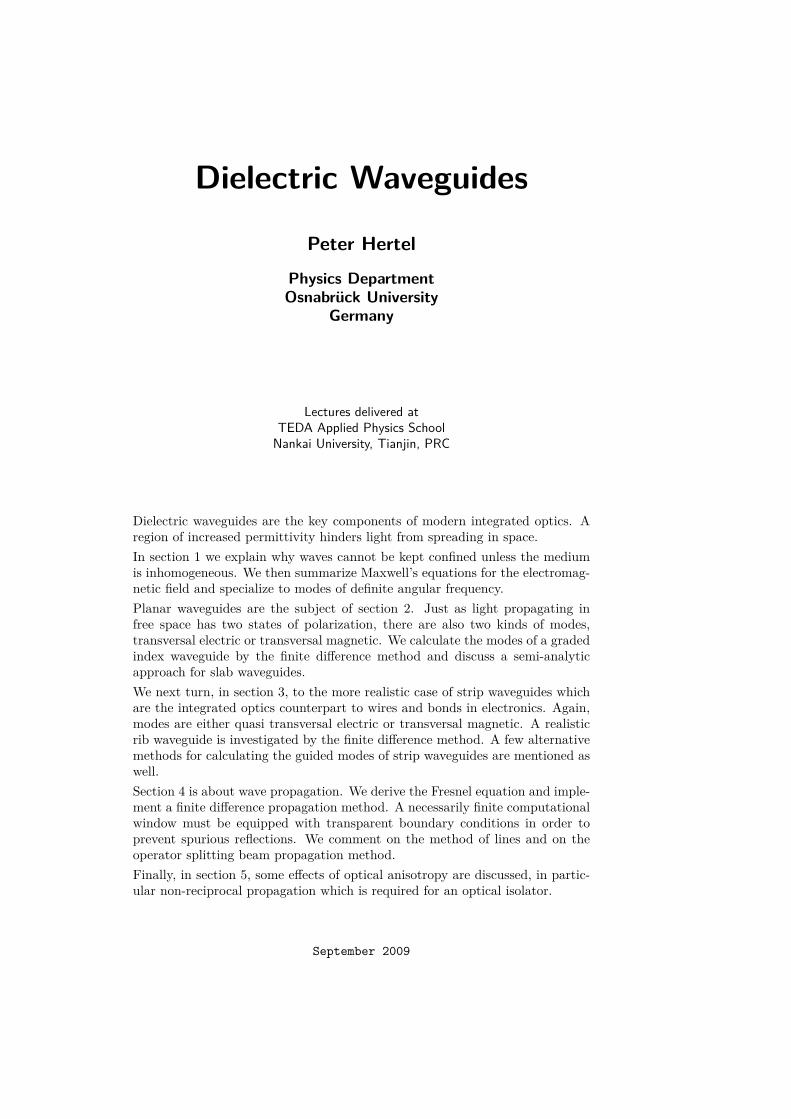
18 eff_eps=diag(eval);19 guided=evec(:,eff_eps>ES);20 plot(x,guided);

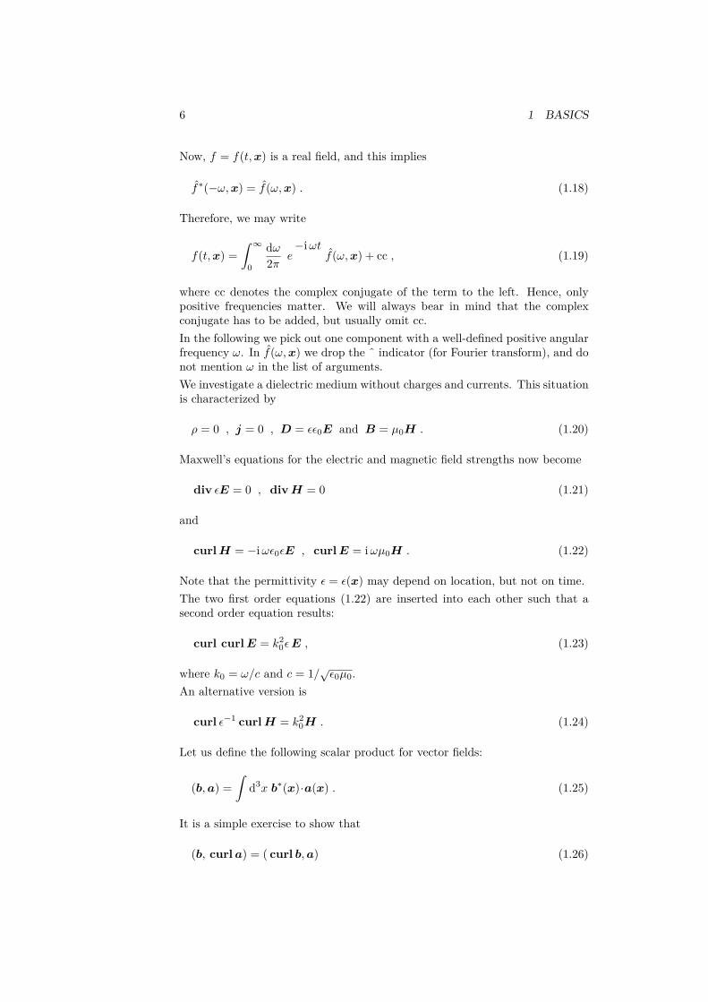
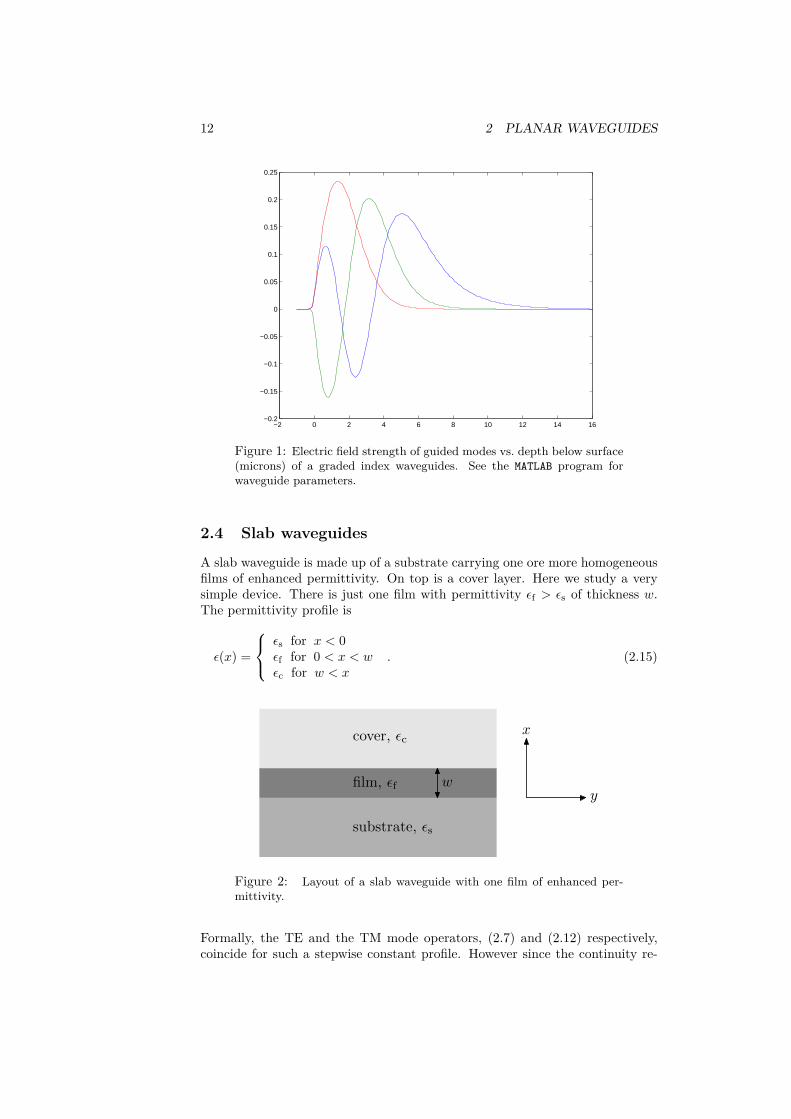
Figure 1 shows the output. There are three guided TE modes which are indexedby TE0, TE1, and TE2. The basic mode, the one with the largest propagationconstant, has no node. The next one has one node, and so forth.On my laptop computer the above program requires 0.3 s to build up the 171×171 matrix, to diagonalize it, and to produce the graphical representation. It issimply not worthwhile to improve it.

12 2 PLANAR WAVEGUIDES

−2 0 2 4 6 8 10 12 14 16−0.2

−0.15

−0.1

−0.05

0

0.05

0.1

0.15

0.2

0.25

Figure 1: Electric field strength of guided modes vs. depth below surface(microns) of a graded index waveguides. See the MATLAB program forwaveguide parameters.

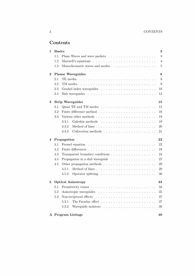
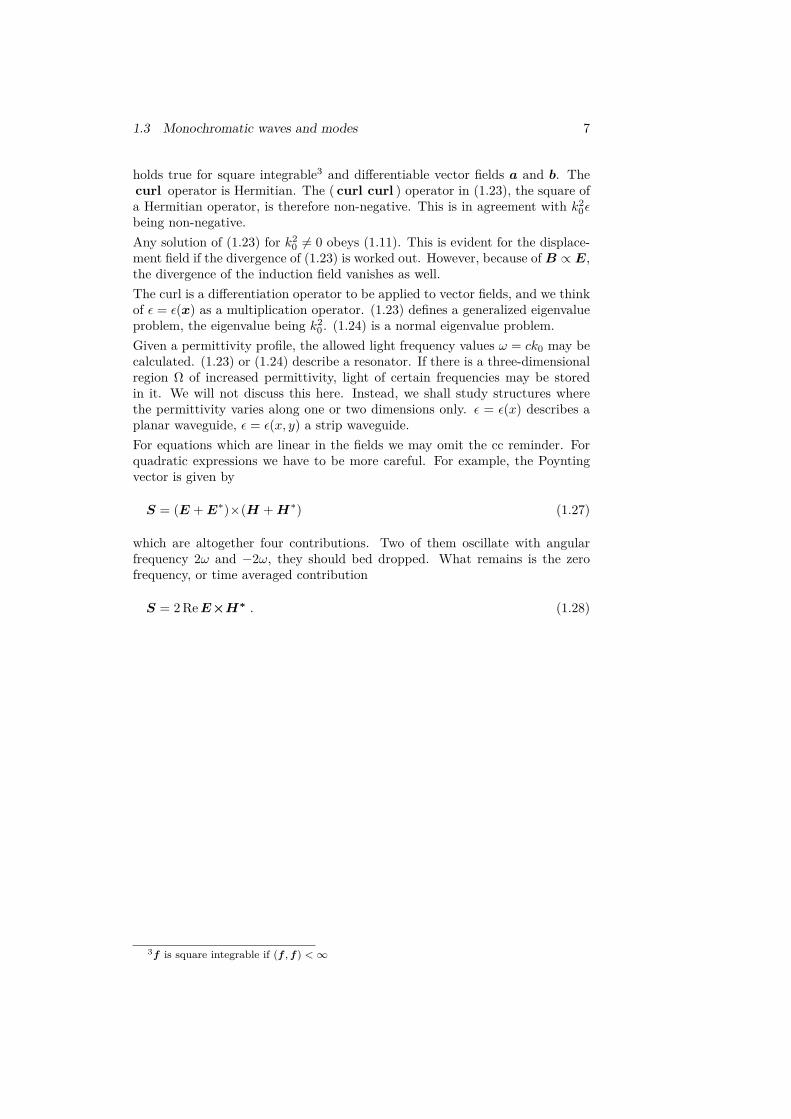
2.4 Slab waveguides

A slab waveguide is made up of a substrate carrying one ore more homogeneousfilms of enhanced permittivity. On top is a cover layer. Here we study a verysimple device. There is just one film with permittivity εf > εs of thickness w.The permittivity profile is

ε(x) =

εs for x < 0εf for 0 < x < wεc for w < x

. (2.15)

y

x

substrate, εs

film, εf

cover, εc

w

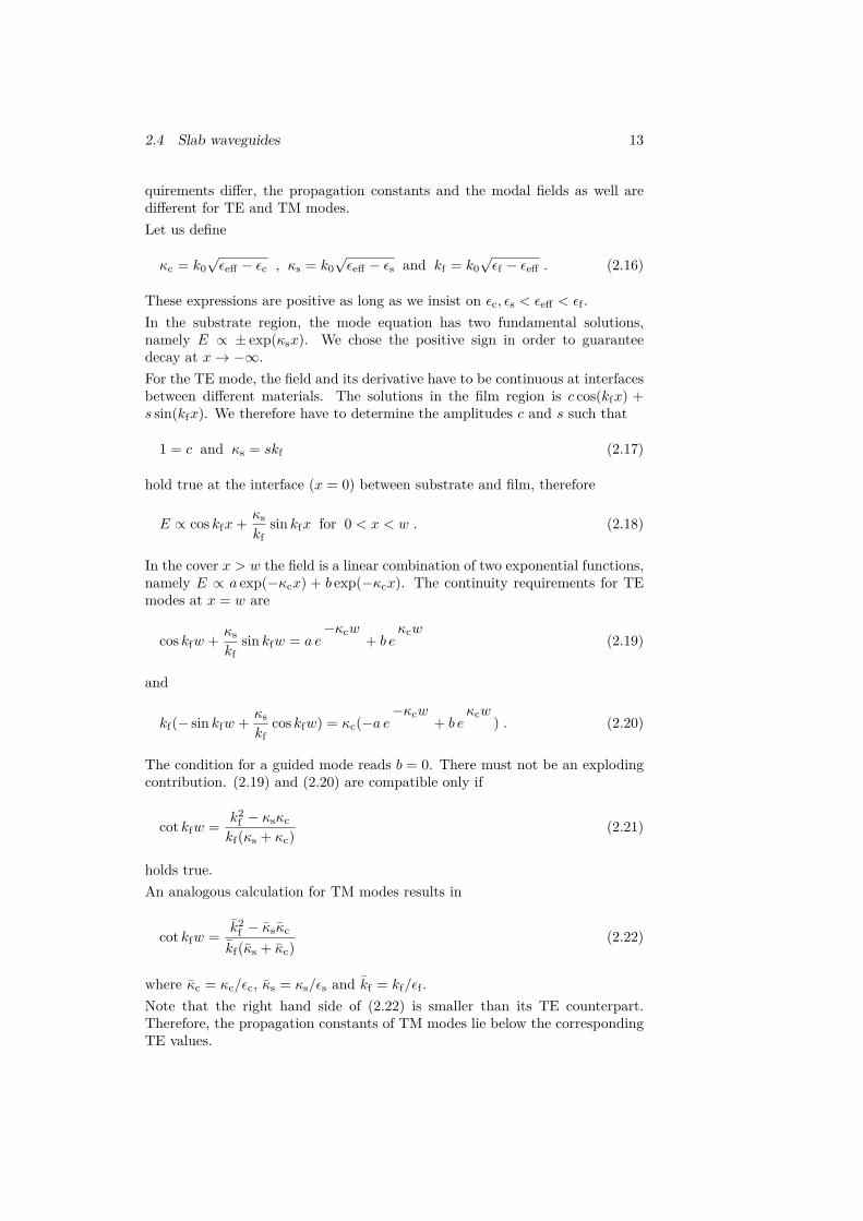
Figure 2: Layout of a slab waveguide with one film of enhanced per-mittivity.

Formally, the TE and the TM mode operators, (2.7) and (2.12) respectively,coincide for such a stepwise constant profile. However since the continuity re-

2.4 Slab waveguides 13

quirements differ, the propagation constants and the modal fields as well aredifferent for TE and TM modes.Let us define

κc = k0√εeff − εc , κs = k0

√εeff − εs and kf = k0

√εf − εeff . (2.16)

These expressions are positive as long as we insist on εc, εs < εeff < εf .In the substrate region, the mode equation has two fundamental solutions,namely E ∝ ± exp(κsx). We chose the positive sign in order to guaranteedecay at x→ −∞.For the TE mode, the field and its derivative have to be continuous at interfacesbetween different materials. The solutions in the film region is c cos(kfx) +s sin(kfx). We therefore have to determine the amplitudes c and s such that

1 = c and κs = skf (2.17)

hold true at the interface (x = 0) between substrate and film, therefore

E ∝ cos kfx+ κskf

sin kfx for 0 < x < w . (2.18)

In the cover x > w the field is a linear combination of two exponential functions,namely E ∝ a exp(−κcx) + b exp(−κcx). The continuity requirements for TEmodes at x = w are

cos kfw + κskf

sin kfw = a e−κcw

+ b eκcw

(2.19)

and

kf(− sin kfw + κskf

cos kfw) = κc(−a e−κcw

+ b eκcw

) . (2.20)

The condition for a guided mode reads b = 0. There must not be an explodingcontribution. (2.19) and (2.20) are compatible only if

cot kfw = k2f − κsκc

kf(κs + κc)(2.21)

holds true.An analogous calculation for TM modes results in

cot kfw = k2f − κsκc

kf(κs + κc)(2.22)

where κc = κc/εc, κs = κs/εs and kf = kf/εf .Note that the right hand side of (2.22) is smaller than its TE counterpart.Therefore, the propagation constants of TM modes lie below the correspondingTE values.

14 2 PLANAR WAVEGUIDES

1.49 1.495 1.5 1.505 1.51 1.515 1.52−4

−3

−2

−1

0

1

2

3

4

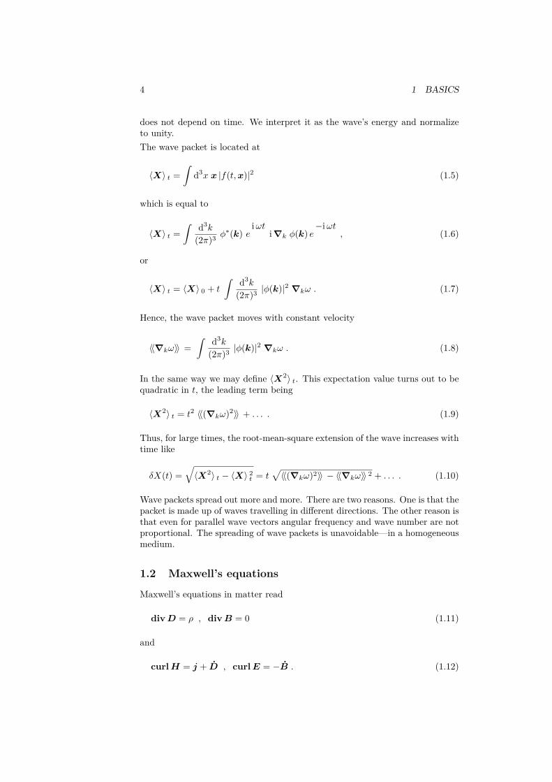
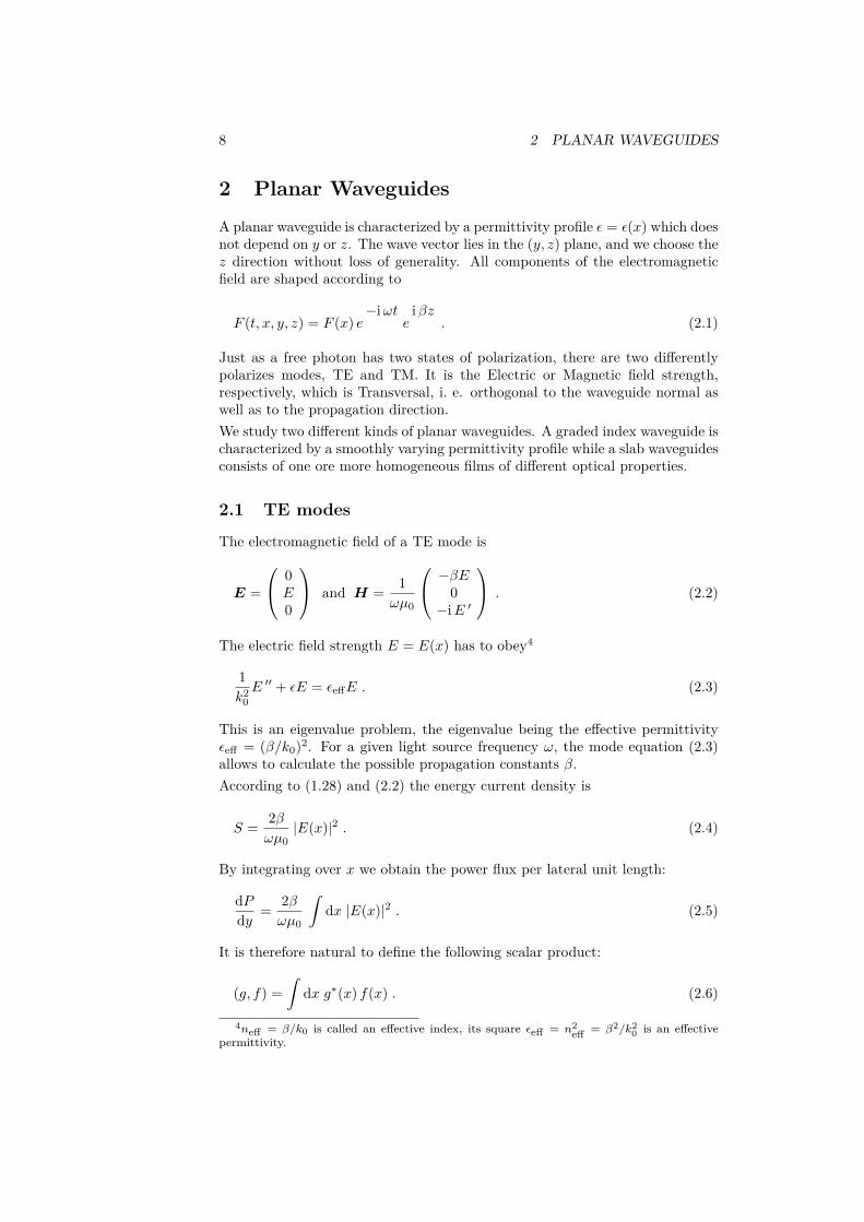
Figure 3: Graphical representation of (2.21) and (2.22). The cotangentas well as the right hand sides are plotted vs. effective index neff . Thefilm (refractive index 1.52, thickness 1.8 microns) is deposited on a glasssubstrate (refractive index 1.49) and covered by air. The simulation isfor a helium-neon laser. There are two guides TE and two guided TMmodes.

Formulae (2.21) or (2.22) allow for an inverse procedure. Assume that at leasttwo TE modes are guided. One can than, for a guessed film refractive indexnf , solve (2.21) for the film thickness w. For each mode i, a film thickness wiresults, but they will coincide only if the guessed film refractive index is correct.If there are more than two modes, the root mean square deviation of calculatedfilm thicknesses must be minimized. Applying the same procedure to TM modesshould result in the same film parameters.

15

3 Strip Waveguides

A linear, or strip waveguide is characterizes by a permittivity profile dependingon the cross section coordinates, ε = ε(x, y). Strip waveguides confine light ina cross section, they are the counterparts of wires for electric currents. Un-like wires, strip waveguides must be rather straight. If the bending radius, ascompared with the waveguide cross section, becomes too small, then power isradiated off or reflected. The latter phenomenon is well known for microwaveguides.Strip waveguides may be produced by depositing on a substrate a thin film ofhigher permittivity and removing it apart from a small rib. This is the mostcommon technique. On lithium niobate a very thin film of titanium is depositedwhich, by common structuring procedures, is removed up to a small rib which isthen in-diffused. Thereby, a smooth permittivity profile ε = ε(x, y) is generated.We look for solutions of Maxwell’s equations of the following form:

F (t, x, y, z) = F (x, y) e−iωt

eiβz

. (3.1)

F may be any component of the electromagnetic field. The mode equation nowis a system of coupled partial differential equations.

3.1 Quasi TE and TM modes

Recall the general mode equation

curl curlE = k20εE . (3.2)

The curl operator is now

curl =

0 −iβ ∂yiβ 0 −∂x−∂y ∂x 0

. (3.3)

Applying it twice results in β2 − ∂2y ∂x∂y iβ∂x

∂x∂y β2 − ∂x∂x iβ∂yiβ∂x iβ∂y −∂2

x − ∂y∂y

E = k20εE . (3.4)

Now, this is a complicated coupled system of partial differential equations. First,because it is redundant: there are three field components, but only two polar-ization states. Second, because the searched for propagation constant β appearslinearly and quadratic, so (3.4) is not a proper eigenvalue problem.Applying the divergence operator results in zero. We therefore may express thez-component of the electric field strength as

−iβEz = ε−1∂xεEx + ε−1∂yεEy . (3.5)

16 3 STRIP WAVEGUIDES

Inserting this into (3.4) gives(k2

0ε+ ∂xε−1∂xε+ ∂2

y ∂xε−1∂yε− ∂x∂y

∂yε−1∂xε− ∂y∂x k2

0ε+ ∂2x + ∂yε

−1∂yε

)(ExEy

)= β2

(ExEy

). (3.6)

This is now a proper eigenvalue problem for β2.In most cases the waveguide is sufficiently broad such that ε∂y ≈ ∂yε is a goodapproximation. If we set Ex ≈ 0 and solve

(∂2x + ∂2

y + k20ε)Ey = β2Ey (3.7)

we have found an approximate solution. It is called a quasi TE mode sincethe normal component of the electrical field strength vanishes, at least approx-imately. (3.7) is the well known Helmholtz equation.The counterpart is a quasi TM mode. It is derived from the alternative waveequation(

k20ε+ ∂2

x + ε∂yε−1∂y ∂x∂y − ε∂yε−1∂x

∂y∂x − ε∂xε−1∂y k20ε+ ε∂xε

−1∂x + ∂2y

)(Hx

Hy

)= β2

(Hx

Hy

). (3.8)

(3.8) results from (1.27) by inserting the mode form (3.1) and eliminating Hz

by making use of ∂xHx + ∂yHy + iβHz = 0.Assuming again ε∂y ≈ ∂yε and setting Hx ≈ 0 results in

(ε∂xε−1∂x + ∂2y + k2

0ε)Hy = β2Hy , (3.9)

a generalized Helmholtz equation.Compare these results with the mode equations for planar waveguides. Now thepermittivity profile and the mode fields depend on the cross section coordinatesx and y. In quasi TE and TM approximation the only change is the additional∂2y operator.

3.2 Finite difference method

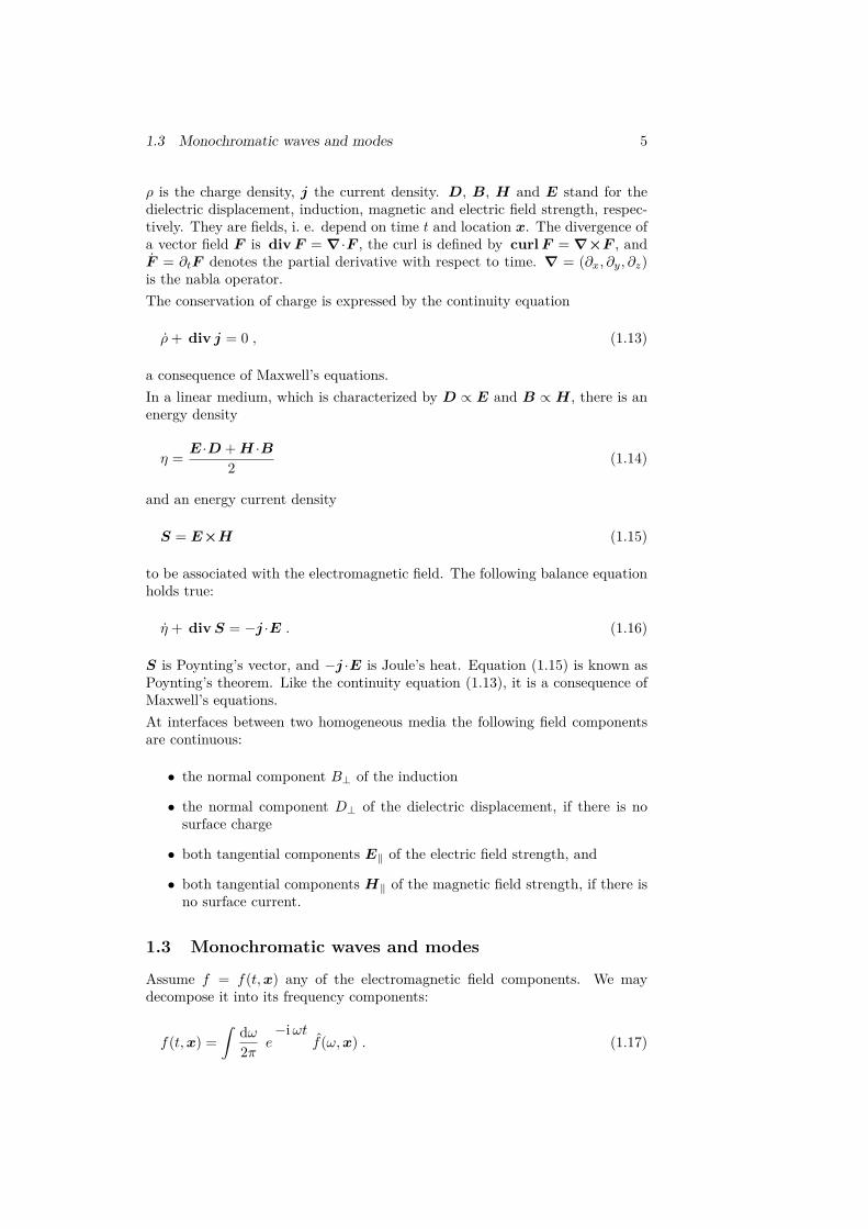
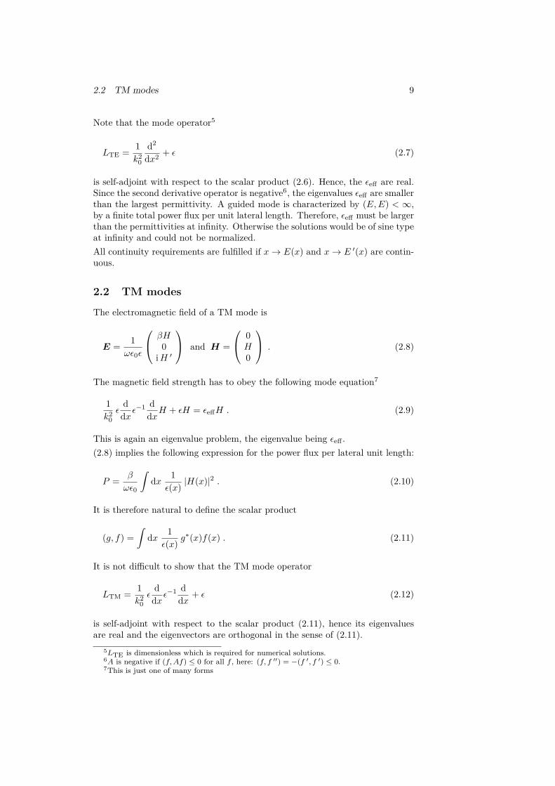
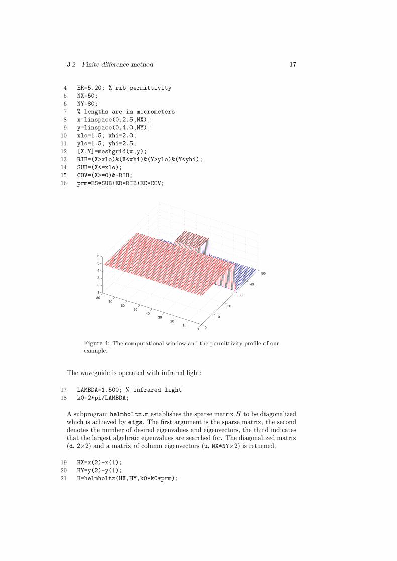
Let us work out a simple example. We want to find out the first two guidedTE modes of a rib waveguide. In order to keep things as simple as possible werefrain from discussing continuity requirements at interfaces between differentmedia, we simply smooth out permittivities there.We choose a computational window the boundaries of which imitate infin-ity. The field has to vanish there. The cross section is represented by points(xi, yj) = (ihx, jhy) within the computational window.The first step is to setup the permittivity profile. We describe a yttrium irongarnet as substrate and a modified garnet as rib. All lengths are in microns.

1 % this file is rib_wg.m2 EC=1.00; % cover permittivity3 ES=3.80; % substrate permittivity

3.2 Finite difference method 17

4 ER=5.20; % rib permittivity5 NX=50;6 NY=80;7 % lengths are in micrometers8 x=linspace(0,2.5,NX);9 y=linspace(0,4.0,NY);

10 xlo=1.5; xhi=2.0;11 ylo=1.5; yhi=2.5;12 [X,Y]=meshgrid(x,y);13 RIB=(X>xlo)&(X<xhi)&(Y>ylo)&(Y<yhi);14 SUB=(X<=xlo);15 COV=(X>=0)&~RIB;16 prm=ES*SUB+ER*RIB+EC*COV;

0

10

20

30

40

50

010

2030

4050

6070

80

1

2

3

4

5

6

Figure 4: The computational window and the permittivity profile of ourexample.

The waveguide is operated with infrared light:

17 LAMBDA=1.500; % infrared light18 k0=2*pi/LAMBDA;

A subprogram helmholtz.m establishes the sparse matrix H to be diagonalizedwhich is achieved by eigs. The first argument is the sparse matrix, the seconddenotes the number of desired eigenvalues and eigenvectors, the third indicatesthat the largest algebraic eigenvalues are searched for. The diagonalized matrix(d, 2×2) and a matrix of column eigenvectors (u, NX*NY×2) is returned.

19 HX=x(2)-x(1);20 HY=y(2)-y(1);21 H=helmholtz(HX,HY,k0*k0*prm);

18 3 STRIP WAVEGUIDES

22 [u,d]=eigs(H,2,’la’);23 mode1=reshape(u(:,1),NX,NY);24 mode2=reshape(u(:,2),NX,NY);

Note that each mesh index pair (i, j) is one running index n. Therefore, the re-sulting eigenvectors mode1 and mode2 have to be reshaped to the computationalwindow.And here comes the code for establishing the Helmholtz operator H = ∆ +d(x, y). The two dimensional Laplacian ∆ = ∂2

x + ∂2y is represented by adding

the expressions for the second derivatives, with possibly different spacing at thetwo dimensions. In general, indices n, n − 1, n + 1, n − Nx and n + Nx arelinked by non-vanishing entries. This does not apply at the borders where thelinks must be set to zero.

1 % this file is helmholtz.m2 function H=helmholtz(HX,HY,d)3 [NX,NY]=size(d’);4 N=NX*NY;5 ihx2=1/HX/HX; ihy2=1/HY/HY;6 md=-2*(ihx2+ihy2)*ones(N,1)+reshape(d’,NX*NY,1);7 xd=ihx2*ones(N,1);8 yd=ihy2*ones(N,1);9 H=spdiags([yd,xd,md,xd,yd],[-NX,-1,0,1,NX],N,N);

10 for n=NX:NX:N-NX11 H(n,n+1)=0;12 H(n+1,n)=0;13 end;

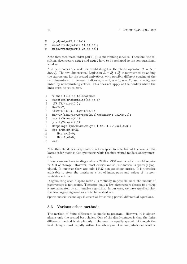
Note that the device is symmetric with respect to reflection at the x-axis. Thelowest order mode is also symmetric while the first excited mode is antisymmet-ric.In our case we have to diagonalize a 2950 × 2950 matrix which would require72 MB of storage. However, most entries vanish, the matrix is sparsely pop-ulated. In our case there are only 14532 non-vanishing entries. It is thereforeadvisable to store the matrix as a list of index pairs and values of its non-vanishing entries.Diagonalizing such a spare matrix is virtually impossible since the matrix ofeigenvectors is not sparse. Therefore, only a few eigenvectors closest to a valueσ are calculated by an iterative algorithm. In our case, we have specified thatthe two largest eigenvalues are to be worked out.Sparse matrix technology is essential for solving partial differential equations.

3.3 Various other methods

The method of finite differences is simple to program. However, it is almostalways only the second best choice. One of the disadvantages is that the finitedifference method is simple only if the mesh is equally spaced. Although thefield changes most rapidly within the rib region, the computational window

3.3 Various other methods 19

0

20

40

60

80

0

10

20

30

40

50−0.04

−0.035

−0.03

−0.025

−0.02

−0.015

−0.01

−0.005

0

0

20

40

60

80

0

10

20

30

40

50−0.04

−0.03

−0.02

−0.01

0

0.01

0.02

0.03

0.04

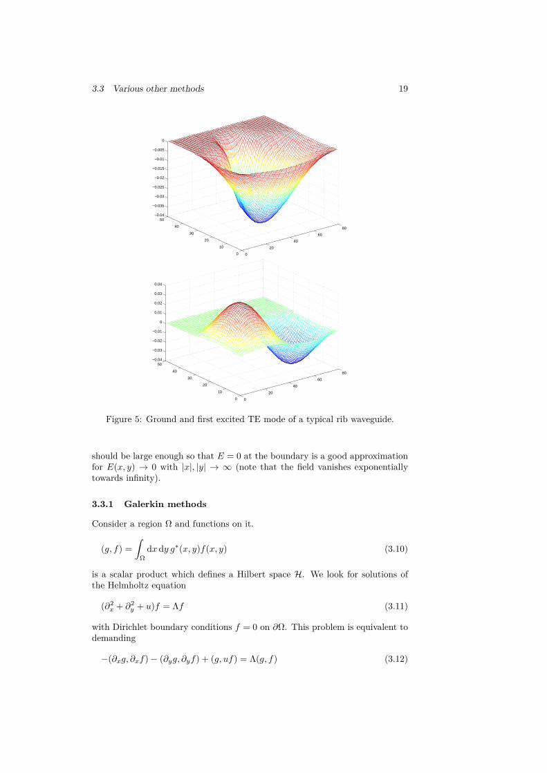
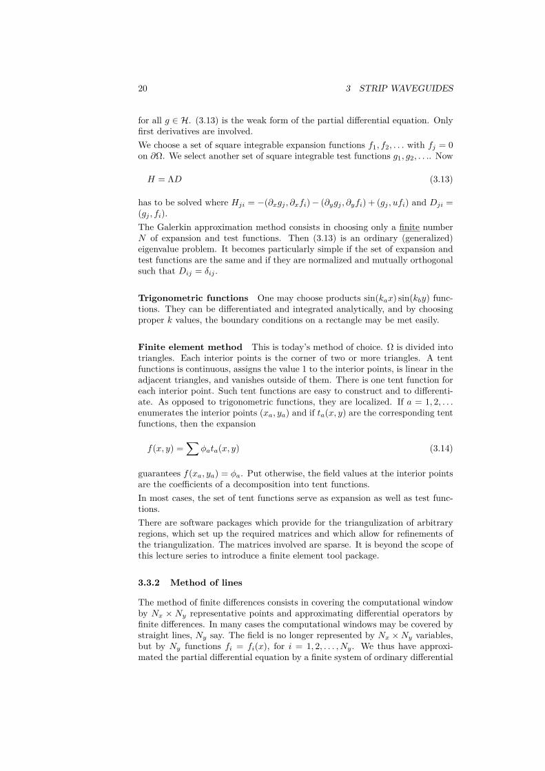
Figure 5: Ground and first excited TE mode of a typical rib waveguide.

should be large enough so that E = 0 at the boundary is a good approximationfor E(x, y) → 0 with |x|, |y| → ∞ (note that the field vanishes exponentiallytowards infinity).

3.3.1 Galerkin methods

Consider a region Ω and functions on it.

(g, f) =∫

Ωdxdy g∗(x, y)f(x, y) (3.10)

is a scalar product which defines a Hilbert space H. We look for solutions ofthe Helmholtz equation

(∂2x + ∂2

y + u)f = Λf (3.11)

with Dirichlet boundary conditions f = 0 on ∂Ω. This problem is equivalent todemanding

−(∂xg, ∂xf)− (∂yg, ∂yf) + (g, uf) = Λ(g, f) (3.12)

20 3 STRIP WAVEGUIDES

for all g ∈ H. (3.13) is the weak form of the partial differential equation. Onlyfirst derivatives are involved.We choose a set of square integrable expansion functions f1, f2, . . . with fj = 0on ∂Ω. We select another set of square integrable test functions g1, g2, . . .. Now

H = ΛD (3.13)

has to be solved where Hji = −(∂xgj , ∂xfi)− (∂ygj , ∂yfi) + (gj , ufi) and Dji =(gj , fi).The Galerkin approximation method consists in choosing only a finite numberN of expansion and test functions. Then (3.13) is an ordinary (generalized)eigenvalue problem. It becomes particularly simple if the set of expansion andtest functions are the same and if they are normalized and mutually orthogonalsuch that Dij = δij .

Trigonometric functions One may choose products sin(kax) sin(kby) func-tions. They can be differentiated and integrated analytically, and by choosingproper k values, the boundary conditions on a rectangle may be met easily.

Finite element method This is today’s method of choice. Ω is divided intotriangles. Each interior points is the corner of two or more triangles. A tentfunctions is continuous, assigns the value 1 to the interior points, is linear in theadjacent triangles, and vanishes outside of them. There is one tent function foreach interior point. Such tent functions are easy to construct and to differenti-ate. As opposed to trigonometric functions, they are localized. If a = 1, 2, . . .enumerates the interior points (xa, ya) and if ta(x, y) are the corresponding tentfunctions, then the expansion

f(x, y) =∑

φata(x, y) (3.14)

guarantees f(xa, ya) = φa. Put otherwise, the field values at the interior pointsare the coefficients of a decomposition into tent functions.In most cases, the set of tent functions serve as expansion as well as test func-tions.There are software packages which provide for the triangulization of arbitraryregions, which set up the required matrices and which allow for refinements ofthe triangulization. The matrices involved are sparse. It is beyond the scope ofthis lecture series to introduce a finite element tool package.

3.3.2 Method of lines

The method of finite differences consists in covering the computational windowby Nx × Ny representative points and approximating differential operators byfinite differences. In many cases the computational windows may be covered bystraight lines, Ny say. The field is no longer represented by Nx ×Ny variables,but by Ny functions fi = fi(x), for i = 1, 2, . . . , Ny. We thus have approxi-mated the partial differential equation by a finite system of ordinary differential

3.3 Various other methods 21

equations which in many cases can be solved quasi-analytically. The method ofline, if applicable, is usually the most precise method although more difficult toprogram than the finite difference method.

3.3.3 Collocation methods

An interesting approach is to expand the searched for solution into products oforthogonal functions which can be differentiated analytically. At suitably chosenpoints the partial differential equation is solved exactly which gives rise to lin-ear equations for the expansion coefficients. In particular, Gauss-Hermite func-tions have been tried which are Gaussians multiplied by polynomials (harmonicoscillator eigenfunctions). The charm of such an expansion is that solutionsautomatically vanish rapidly at infinity, as they should.However, there is a serious flaw. Orthogonal polynomials necessarily have co-efficients of alternating sign. The small sum is the result of an almost totalcancellation of large contributions, and by a rule of thumb, not more than60 terms can be summed before running into serious rounding error problems.

22 4 PROPAGATION

4 Propagation

So far we have discussed guided modes. They have definite propagation con-stants and are either TE or TM polarized. In many cases, however, modeanalysis is not sufficient, either because the structure under study is not z-homogeneous or because energy is radiated off. In this section we want todescribe the propagation of a beam. For simplicity, the scalar equation of aquasi TE polarized wave is discussed.

4.1 Fresnel equation

We relax the requirement that the field is a plane wave with respect to propa-gation along the z axis. Instead we write

E(t, x, y, z) = e−iωt

eink0z

E(x, y; z) . (4.1)

β = nk0 is the carrier spatial frequency, it should be chosen such that E(x, y; z)depends as weakly as possible on the propagation coordinate z. Put otherwise:we discuss situations where light is almost a mode travelling in z direction.We have to solve the following wave equations8:

e−ink0z

(∂2x + ∂2

y + d2

dz2 ) eink0z

E(z) + k20εE(z) = 0 . (4.2)

Because the fields E(z) are assumed to depend but weakly on z, we neglect itssecond derivative. The result is

−iE ′(z) = P E(z) where P =∂2x + ∂2

y − k20 δε

2nk0, (4.3)

the well-known Fresnel equation, with δε(x, y) = ε(x, y)− n2. P is an operatoracting on fields x, y → f(x, y).(4.3) is not of second, but of first order with respect to propagation: by insistingon a weak z-dependency of E(z) we have singled out the forward propagatingbeam.The Fresnel equation describes the propagation of a beam well provided n ischosen properly, namely such that

||E ′′(z)|| k0||E ′(z)|| (4.4)

holds true9.Note that in a homogeneous medium E(x, y; z) = A is a solution if n2 = ε. Thisdescribes a plane wave travelling in z direction.In the following subsections we discuss various methods how to solve the Fresnelequation.

8x, y → E(x, y; z) is regarded as a family of fields being parameterized by z9The norm of a field is defined by ||f ||2 =

∫dxdy |f(x, y)|2

4.2 Finite differences 23

4.2 Finite differences

Let us assume that ε = ε(x, y) does not depend on the propagation coordinate z.In this case (4.3) is formally solved by

E(z) = e−i zP

E(0) (4.5)

or, discussing a propagation step h,

E(z + h) = e−ihP

E(z) . (4.6)

A very crude approximation is

E(z + h) = (I − ihP )E(z) . (4.7)

Likewise, one may write

eihP

E(z + h) = E(z) (4.8)

and approximate by

E(z + h) = (I + ihP )−1E(z) . (4.9)

We assume that the operator P is also represented by a finite difference schemeon the cross section x, y. It turns out that propagating forward in time by(4.7) is unstable. Sending all propagation steps to zero so that more and morepropagation steps are required does not converge. Propagating backward intime by (4.9) is more cumbersome because a system of linear equations has tobe solved, however, the method is stable. Both are of first order in h.A combination of the two methods is one order more accurate and stable aswell. We set

E(z + h

2 ) = (I − ihP2 )E(z) = (I + ihP

2 )E(z + h) (4.10)

and obtain

E(z + h) = (I + ihP2 )−1 (I − ihP

2 )E(z) , (4.11)

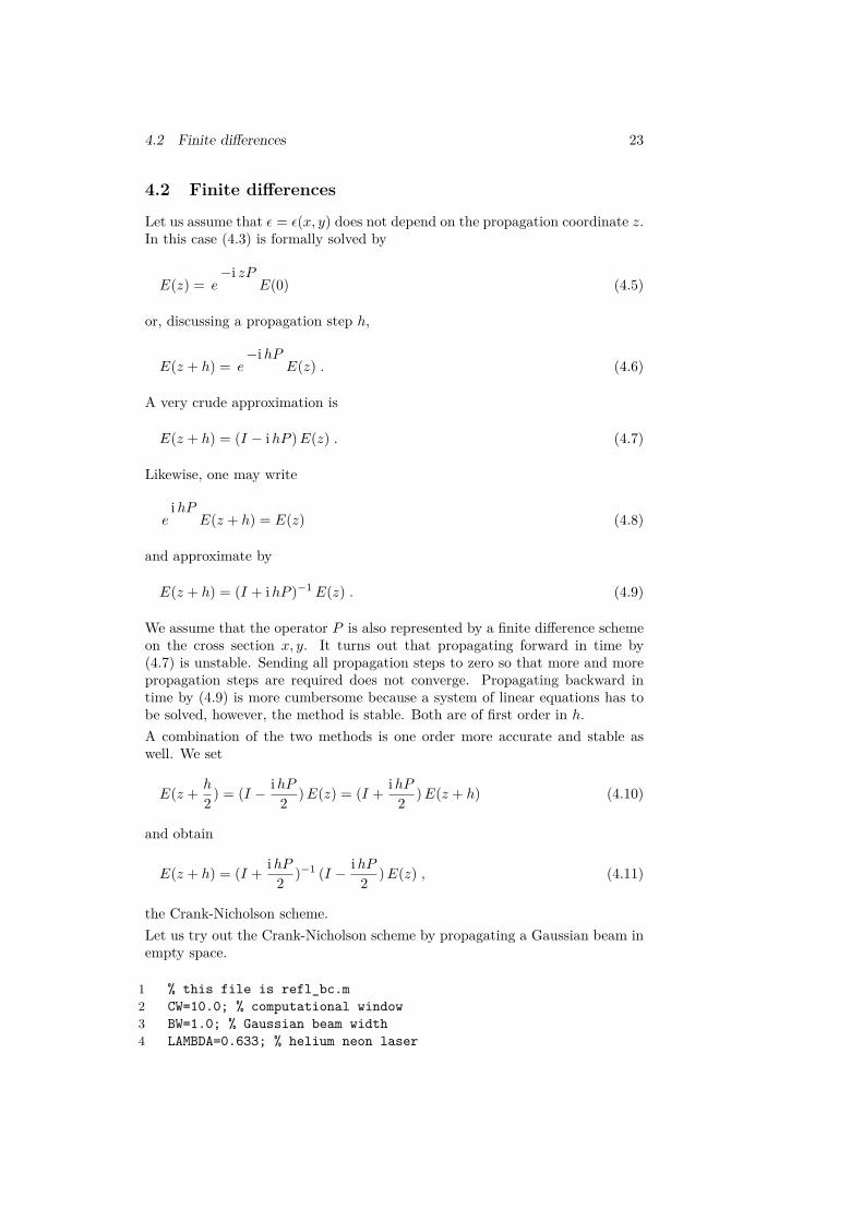
the Crank-Nicholson scheme.Let us try out the Crank-Nicholson scheme by propagating a Gaussian beam inempty space.

1 % this file is refl_bc.m2 CW=10.0; % computational window3 BW=1.0; % Gaussian beam width4 LAMBDA=0.633; % helium neon laser

24 4 PROPAGATION

5 n=1.0; % refractive index of the medium6 k0=2*pi/LAMBDA;7 NX=128; % points on x axis8 HX=CW/(NX-1); % x axis spacing9 HZ=5*HX; % propagation step

10 x=linspace(-0.5*CW,0.5*CW,NX)’;11 E=exp(-(x/BW).^2); % initial field12 u=0.5i*HZ/(2*n*k0);13 main=-2*u*ones(NX,1)/HX^2;14 next=u*ones(NX-1,1)/HX^2;15 % step forward16 FW=eye(NX)+diag(next,-1)+diag(main,0)+diag(next,1);17 % step backward18 BW=eye(NX)-diag(next,-1)-diag(main,0)-diag(next,1);19 NZ=100; % number of propagation steps20 hist=zeros(NX,NZ); % storage for history21 for r=1:NZ22 hist(:,r)=abs(E).^2;23 E=BW\FW*E;24 end;

020

4060

80100

0

50

100

1500

0.2

0.4

0.6

0.8

1

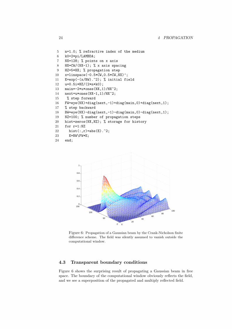
Figure 6: Propagation of a Gaussian beam by the Crank-Nicholson finitedifference scheme. The field was silently assumed to vanish outside thecomputational window.

4.3 Transparent boundary conditions

Figure 6 shows the surprising result of propagating a Gaussian beam in freespace. The boundary of the computational window obviously reflects the field,and we see a superposition of the propagated and multiply reflected field.

4.3 Transparent boundary conditions 25

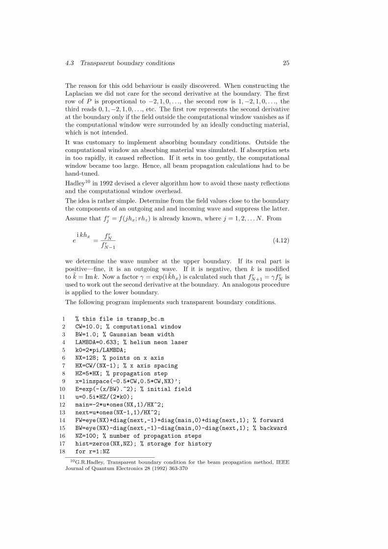
The reason for this odd behaviour is easily discovered. When constructing theLaplacian we did not care for the second derivative at the boundary. The firstrow of P is proportional to −2, 1, 0, . . ., the second row is 1,−2, 1, 0, . . ., thethird reads 0, 1,−2, 1, 0, . . ., etc. The first row represents the second derivativeat the boundary only if the field outside the computational window vanishes as ifthe computational window were surrounded by an ideally conducting material,which is not intended.It was customary to implement absorbing boundary conditions. Outside thecomputational window an absorbing material was simulated. If absorption setsin too rapidly, it caused reflection. If it sets in too gently, the computationalwindow became too large. Hence, all beam propagation calculations had to behand-tuned.Hadley10 in 1992 devised a clever algorithm how to avoid these nasty reflectionsand the computational window overhead.The idea is rather simple. Determine from the field values close to the boundarythe components of an outgoing and and incoming wave and suppress the latter.Assume that frj = f(jhx; rhz) is already known, where j = 1, 2, . . . N . From

ei khx

= frNfrN−1

(4.12)

we determine the wave number at the upper boundary. If its real part ispositive—fine, it is an outgoing wave. If it is negative, then k is modifiedto k = Im k. Now a factor γ = exp(i khx) is calculated such that frN+1 = γfrN isused to work out the second derivative at the boundary. An analogous procedureis applied to the lower boundary.The following program implements such transparent boundary conditions.

1 % this file is transp_bc.m2 CW=10.0; % computational window3 BW=1.0; % Gaussian beam width4 LAMBDA=0.633; % helium neon laser5 k0=2*pi/LAMBDA;6 NX=128; % points on x axis7 HX=CW/(NX-1); % x axis spacing8 HZ=5*HX; % propagation step9 x=linspace(-0.5*CW,0.5*CW,NX)’;

10 E=exp(-(x/BW).^2); % initial field11 u=0.5i*HZ/(2*k0);12 main=-2*u*ones(NX,1)/HX^2;13 next=u*ones(NX-1,1)/HX^2;14 FW=eye(NX)+diag(next,-1)+diag(main,0)+diag(next,1); % forward15 BW=eye(NX)-diag(next,-1)-diag(main,0)-diag(next,1); % backward16 NZ=100; % number of propagation steps17 hist=zeros(NX,NZ); % storage for history18 for r=1:NZ

10G.R.Hadley, Transparent boundary condition for the beam propagation method, IEEEJournal of Quantum Electronics 28 (1992) 363-370

26 4 PROPAGATION

19 hist(:,r)=abs(E).^2;20 E=one_step(HX,u,FW,BW,1e-4,E);21 end;

020

4060

80100

0

50

100

1500

0.2

0.4

0.6

0.8

1

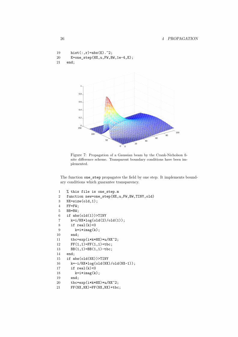
Figure 7: Propagation of a Gaussian beam by the Crank-Nicholson fi-nite difference scheme. Transparent boundary conditions have been im-plemented.

The function one_step propagates the field by one step. It implements bound-ary conditions which guarantee transparency.

1 % this file is one_step.m2 function new=one_step(HX,u,FW,BW,TINY,old)3 NX=size(old,1);4 FF=FW;5 BB=BW;6 if abs(old(1))>TINY7 k=i/HX*log(old(2)/old(1));8 if real(k)<09 k=i*imag(k);

10 end;11 tbc=exp(i*k*HX)*u/HX^2;12 FF(1,1)=FF(1,1)+tbc;13 BB(1,1)=BB(1,1)-tbc;14 end;15 if abs(old(NX))>TINY16 k=-i/HX*log(old(NX)/old(NX-1));17 if real(k)<018 k=i*imag(k);19 end;20 tbc=exp(i*k*HX)*u/HX^2;21 FF(NX,NX)=FF(NX,NX)+tbc;

4.4 Propagation in a slab waveguide 27

22 BB(NX,NX)=BB(NX,NX)-tbc;23 end;24 new=BB\FF*old;

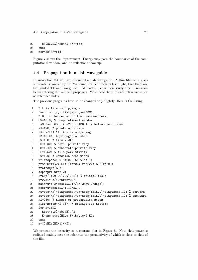
Figure 7 shows the improvement. Energy may pass the boundaries of the com-putational window, and no reflections show up.

4.4 Propagation in a slab waveguide

In subsection 2.4 we have discussed a slab waveguide. A thin film on a glasssubstrate is covered by air. We found, for helium-neon laser light, that there aretwo guided TE and two guided TM modes. Let us now study how a Gaussianbeam entering at z = 0 will propagate. We choose the substrate refractive indexas reference index.The previous programs have to be changed only slightly. Here is the listing:

1 % this file is prp_swg.m2 function [x,z,hist]=prp_swg(BC);3 % BC is the center of the Gaussian beam4 CW=10.0; % computational window5 LAMBDA=0.633; k0=2*pi/LAMBDA; % helium neon laser6 NX=128; % points on x axis7 HX=CW/(NX-1); % x axis spacing8 HZ=10*HX; % propagation step9 FW=1.8; % film width

10 EC=1.00; % cover permittivity11 ES=1.49; % substrate permittivity12 EF=1.52; % film permittivity13 BW=1.0; % Gaussian beam width14 x=linspace(-0.5*CW,0.5*CW,NX)’;15 prm=ES*(x<0)+EF*((x>=0)&(x<=FW))+EC*(x>FW);16 nref=sqrt(ES);17 deps=prm-nref^2;18 E=exp(-((x-BC)/BW).^2); % initial field19 u=0.5i*HZ/(2*nref*k0);20 main=u*(-2*ones(NX,1)/HX^2+k0^2*deps);21 next=u*ones(NX-1,1)/HX^2;22 FW=eye(NX)+diag(next,-1)+diag(main,0)+diag(next,1); % forward23 BW=eye(NX)-diag(next,-1)-diag(main,0)-diag(next,1); % backward24 NZ=250; % number of propagation steps25 hist=zeros(NX,NZ); % storage for history26 for r=1:NZ27 hist(:,r)=abs(E).^2;28 E=one_step(HX,u,FW,BW,1e-4,E);29 end;30 z=[0:HZ:(NZ-1)*HZ];

We present the intensity as a contour plot in Figure 8. Note that power isradiated mainly into the substrate the permittivity of which is close to that ofthe film.

28 4 PROPAGATION

0 20 40 60 80 100 120 140 160 180−5

−4

−3

−2

−1

0

1

2

3

4

5

Figure 8: A Gaussian beam is inserted into a slab waveguide. The beamcenter is at the middle of the film. Propagation is from left to right.

0 20 40 60 80 100 120 140 160 180 2000.88

0.9

0.92

0.94

0.96

0.98

1

1.02

Figure 9: Power within the computational window vs. propagation dis-tance for the previous propagation calculation.

It is interesting to study the power within the computational window which wehave depicted in Figure 9. For a short distance it remains constant because thebeam has not yet reached the boundaries of the computational window. It thenfalls off, and after a certain length it becomes constant because the mode is wellguided within the computational window. About 11% of the original power areradiated off.

4.5 Other propagation methods 29

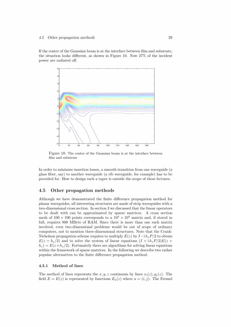
If the center of the Gaussian beam is at the interface between film and substrate,the situation looks different, as shown in Figure 10. Now 27% of the incidentpower are radiated off.

0 20 40 60 80 100 120 140 160 180−5

−4

−3

−2

−1

0

1

2

3

4

5

Figure 10: The center of the Gaussian beam is at the interface betweenfilm and substrate

In order to minimize insertion losses, a smooth transition from one waveguide (aglass fiber, say) to another waveguide (a rib waveguide, for example) has to beprovided for. How to design such a taper is outside the scope of these lectures.

4.5 Other propagation methods

Although we have demonstrated the finite difference propagation method forplanar waveguides, all interesting structures are made of strip waveguides with atwo-dimensional cross section. In section 3 we discussed that the linear operatorsto be dealt with can be approximated by sparse matrices. A cross sectionmesh of 100 × 100 points corresponds to a 104 × 104 matrix and, if stored infull, requires 800 MByte of RAM. Since there is more than one such matrixinvolved, even two-dimensional problems would be out of scope of ordinarycomputers, not to mention three-dimensional structures. Note that the Crank-Nicholson propagation scheme requires to multiply E(z) by I−ihzP/2 to obtainE(z + hz/2) and to solve the system of linear equations (I + ihzP/2)E(z +hz) = E(z+hz/2). Fortunately there are algorithms for solving linear equationswithin the framework of sparse matrices. In the following we describe two ratherpopular alternatives to the finite difference propagation method.

4.5.1 Method of lines

The method of lines represents the x, y, z continuum by lines xi(z), yj(z). Thefield E = E(z) is represented by functions Ea(z) where a = (i, j). The Fresnel

30 4 PROPAGATION

equation now reads

−iE ′a =∑b

PabEb(z) . (4.13)

This is a set of coupled ordinary differential equations, although a mighty set.The standard procedure to solve it is by diagonalizing the P matrix whichrepresents the Fresnel operator on the waveguide cross section. We may write

Pab =∑c

U†acpcUcb , (4.14)

where U is a unitary matrix because P is Hermitian. Ea =∑b UabEb now is

subject to a set of uncoupled differential equations

−i E ′a = paEa (4.15)

the solution of which is

Ea(z) = ei paz

Ea(0) (4.16)

or

Ea(z) =∑b

U†ab ei pbz

UbaEa(0) . (4.17)

As said above, working out the exponential of iPz by diagonalization is pro-hibitive for two-dimensional cross section. A few of the eigenvalues correspond toguided modes, the remaining thousands of eigenvalues refer to radiation modes.Incoming radiation has to be suppressed, outgoing radiation may be representedby a few lossy modes. By a tricky balance between simplicity, storage require-ment, run-time and accuracy the method of lines has proven to be a seriousalternative to the finite difference method.

4.5.2 Operator splitting

This is the oldest beam propagation scheme11. It is tailored to the computa-tional facilities of more than 30 years ago: random access memory was shortand had to be replaced by long program run times. There is an intuitive and amathematical foundation.The Fresnel propagation operator consists of two parts. The first one is a crosssection Laplacian which describes propagation in free space. As we know, anybeam of light diverges when propagating in free space. The second contributioncharacterizes focussing. The guiding structure has a higher refractive index thanthe surrounding. The optical path through the centre of a lens is shorter thanan off-axis optical path which effect leads to focussing. The Fresnel equationdescribes propagation in free space and focussing in infinitely rapid succession.

11J. A. Fleck, J. R. Morris, M. D. Feit: Appl. Phys. 10 (1976) 129

4.5 Other propagation methods 31

We approximate it by finite steps of propagation in free space and focussing bya permittivity profile.Mathematically, the Fresnel propagation operator P = D + M is the sum of adifferential operator

D =∂2x + ∂2

y

2nk0(4.18)

and a multiplication operator

M = k0δε

2n . (4.19)

Recall that n is a reference index and δε = ε(x, y) − n2. Both act on fieldsdepending on the cross section coordinates x, y.D describes the propagation in a homogeneous medium of refractive index nwhile M characterizes the focussing effect. These operators do not commute,and the rule exp(A+B) = exp(A) exp(B) is not applicable.However,

eihz(D +M)

≈ eihzD/2

eihzM

eihzD/2

(4.20)

is an approximation, the error being proportional to h3z.

The operator splitting expression, as given by the right hand side of (4.20), isapplied as follows.The field is Fourier transformed,

E1(kx, ky) =∫

dxdy ei (xkx + yky)

E1(x, y) . (4.21)

Then

E2(kx, ky) = e−ihz(k2

x + k2y)/4nk0

E1(kx, ky) (4.22)

is calculated. Fourier back transformation yields

E2(x, y) =∫ dkx

2πdky2π e

−i (xkx + yky)E2(kx, ky) . (4.23)

We now set

E3(x, y) = eihzk0δε(x, y)/2n

E2(x, y) (4.24)

and Fourier transform to

E3(kx, ky) =∫

dxdy ei (xkx + yky)

E3(x, y) . (4.25)

32 4 PROPAGATION

Finally,

E4(kx, ky) = e−ihz(k2

x + k2y)/2nk0

E3(kx, ky) (4.26)

is worked out which is the last part of the first propagation step and the first partof the next. This sequence of operations is continued with possibly modifyingδε if the structure changes along the propagation direction.Note that the method of operator splitting requires no additional storage formatrices but depends on a fast Fourier transform algorithm. Also note that eachsingle propagation step is described by applying a unitary matrix. Hence, thenorm ||E|| of the original field remains constant. Without transparent boundaryconditions or another means to avoid reflections the operating splitting propa-gation method runs into the same problems as discussed earlier.

33

5 Optical Anisotropy

Up to now we always assumed that the electrical field strength E and the di-electric displacement D were parallel. This is true for optically isotropic media,like glass, silicon, or other cubic crystals or amorphous substances. Therefore,we always talked about permittivity as a scalar, as in Di = εε0Ei. In generalit is still true that, for sufficiently small electric fields, displacement and fieldstrength are proportional, but they are not necessarily parallel. We thereforehave to write12 Di = εijε0Ej , with the permittivity tensor εij . This sectiondiscusses effects of optical anisotropy.

5.1 Permittivity tensor

We talk about a system of particles at xa with charge qa. The polarization atx is

Pi(x) =∑a

qaxiδ3(x− xa) . (5.1)

Denote by H the Hamiltonian of matter which is perturbed by the interactionwith an electric field E(t,x). The Hamiltonian now is

Ht = H −∫

d3xPi(x)Ei(t,x) . (5.2)

We assume that the system was in a Gibbs state

G = e(F −H)/kBT

(5.3)

before the perturbation has set in. F is the free energy, kB denotes Boltzmann’sconstant, and T is the temperature of the equilibrium state.Within the framework of linear response theory, the effect of the perturbationon the polarization may be worked out:

Pi(t,x) =∫ ∞

0dτ∫

d3ξ Γij(τ, ξ)Ej(t− τ,x− ξ) . (5.4)

Here Pi(t,x) = 〈Pi(x)〉 t is the expectation value of the polarization in thetime-dependent perturbed state. The Green’s function Γij is found to be

Γij(τ, ξ) = 〈 i~

[U−τPi(ξ)Uτ , Pj(0) ]〉 (5.5)

where Ut denotes time translation by the unperturbed Hamiltonian,

Ut = e−i tH/~

. (5.6)12Einstein’s summation convention: a sum over doubly occurring indices is silently under-

stood.

34 5 OPTICAL ANISOTROPY

The expectation value in (5.5) is with the unperturbed Hamiltonian. Put oth-erwise, the unperturbed system knows how to react on a perturbation.By Fourier transforming all quantities13 we arrive at

Pi(ω, q) = ε0χij(ω, q) Ej(ω, q) (5.7)

where the susceptibility tensor χji is

χij(ω, q) = 1ε0

∫ ∞0

dτ eiωτ ∫

d3ξ e−i q ·ξ

Γij(τ, ξ) . (5.8)

The permittivity εij = δij +χij can thus be calculated, in principle. It dependson angular frequency ω, on a wave vector q, and on all parameters which enterthe Gibbs state, such as temperature or quasi-static external fields.Matter in its solid state has a time scale which is governed by the speed ofsound. Since this is so much smaller than the speed of light, we may write

χij(ω, q) = χ(0)ij (ω) + χ

(1)ijkqk + . . . . (5.9)

The first contribution is the ordinary susceptibility, it depends on angular fre-quency only. The second term describes optical activity. It is responsible forrotating the polarization vector of a linearly polarized wave by a few degreesper centimeter which is a tiny effect. We will not discuss optical activity hereand denote the susceptibility by χij(ω) = χ0

ij(ω) henceforth.The permittivity should be split into a Hermitian and an anti-Hermitian con-tribution, εij = ε ′ij + i ε ′′ij . The Hermitian, or refractive part ε ′ is responsiblefor refraction, for the bending of light rays. The anti-Hermitian, or absorptivecontribution ε ′′ causes absorption. The dissipation-fluctuation theorem assuresthat ε ′′ is non-negative in accordance with the second law of thermodynamics:light energy is transformed into heat, the opposite is impossible.The refractive and absorptive parts of the permittivity tensor are not indepen-dent, they obey the Kramer-Kronigs dispersion relation

ε ′ij(ω) = δij +∫ du

π

ε ′′ij(u)u− ω

, (5.10)

where the principal value integral is understood. There is no refraction withoutabsorption. It is however possible that the absorptive part of the permittiv-ity tensor almost vanishes in an entire frequency range. We then speak of atransparency window.Let us mention another useful relation which can be derived by studying (5.5)with respect to time reversal. It turns out that the permittivity is a symmetrictensor provided that an external magnetic field is reversed. Denoting external,or quasi-static fields by E and B, Onsager’s relations amount to

εij(ω, E, B) = εji(ω, E,−B) . (5.11)13The Fourier transform of a convolution is the product of the Fourier transforms.

5.2 Anisotropic waveguides 35

5.2 Anisotropic waveguides

We assume a material without magneto-optic effect. By Onsager’s relationthe permittivity tensor is symmetric and can be diagonalized by an orthogonalcoordinate transformation. We assume the axes of the coordinate system tocoincide with the optical axes. In this case the permittivity is a diagonal matrixwith entries εx, εy, εz.Let us comment first on slab waveguides.Our previous analysis, that there are TE and TM modes, remains valid.

E =

0E0

and H = 1iωµ0

−iβE0E ′

(5.12)

solves Maxwell’s equations provided the TE mode equation

E ′′ + k20εyE = β2E (5.13)

is satisfied. E and E ′ have to be continuous.Likewise,

E = 1−iωε0

−iβH/εx0H ′/εz

and H =

0H0

(5.14)

solve all Maxwell equations if the TM mode equation

εxd

dxε−1z

d

dxH + k20εxH = β2H (5.15)

holds true. H and H ′/εz must be continuous.For strip waveguides the mode equations become very complicated, and werefrain from discussing the various approximation schemes which have been putforward. The deviations from isotropy are usually rather small and may bedealt with as a perturbation.So let us discuss a waveguide with permittivity

εij = εδij + ∆εij . (5.16)

For the following discussion the inverse tensor

ηij = η + ∆ηij (5.17)

is the more suitable quantity, where η = 1/ε and ∆ηij = −∆εij/ε2.The wave equation to be solved is (1.24), namely

curl ε−1 curlH = LH = k20H , (5.18)

36 5 OPTICAL ANISOTROPY

where

curl =

0 −iβ ∂yiβ 0 −∂x−∂y ∂x 0

(5.19)

is the curl operator for a strip waveguide. Note that η in (5.18) is a tensor.We define the following scalar product for vector fields:

(g,f) =∫

dxdy g∗i (x, y) fi(x, y) . (5.20)

With this scalar product, the curl operator is symmetric. Since we assume atransparent medium, the permittivity tensor is Hermitian, and so is η. It followsthat the mode operator L is also symmetric. Its eigenvalues k2

0 may be obtainedfrom

k20 = ( curlH, η curlH)

(H,H) = Φ(H) . (5.21)

We have introduced in (5.21) a functional f → Φ(f) of vector fields. It is asimple exercise to show that Φ is stationary at mode fields:

d

dsΦ(H + s δH )

∣∣∣∣s=0

= 0 . (5.22)

Now, the eigenvalues k20 of (5.21) depend twofold on ∆η, directly and indirectly

via the dependency of the mode fields on the inverse permittivity. The lattereffect, however, vanishes because the functional Φ is stationary at solutions ofthe wave equation. Therefore

∆k20 = ( curlH,∆η curlH)

(H,H) (5.23)

holds true in first order perturbation theory.This change in ∆k2

0 must be compensated by a shift ∆β of the propagationconstant:

∆k20 + dk2

0dβ2 ∆β2 = 0 (5.24)

where we again may exploit that the derivative dk20/dβ

2 does not depend im-plicitly on β. With

dk20

dβ2 =

∫dx dy η(H2

x +H2y )∫

dxdy (H2x +H2

y +H2z )

(5.25)

5.3 Non-reciprocal effects 37

we finally arrive at

∆β = − 12β

∫dxdy curlHi ∆ηij curlHj∫

dxdy η (H2x +H2

y ). (5.26)

There are many variations of this formula. The effect of anisotropy on the prop-agation constant may be expressed in the electric fields, this or that componentcan be removed by the divergence equation or because it is small, and so forth.(5.26) however is free from unnecessary approximations.

5.3 Non-reciprocal effects

We discuss in this subsection a special, but most important optical anisotropy,namely the Faraday effect. We shall explain why magnetism must be involvedto achieve non-reciprocal light propagation.

5.3.1 The Faraday effect

Maxwell’s equation ε0 divE = ρ, divB = 0, curlB/µ0 = j + ε0E andcurlE = −B are compatible with time reversal. If E,B, ρ and j is a solution,then E? = E,B? = −B, ρ? = ρ and j? = −j is a solution as well, wheref?(t,x) = f(−t,x). It can be seen from S = E×H that time reversal impliesthe reversal of motion. If there is a wave travelling in forward direction, thereis an identical wave travelling backward. Not quite. The magnetic field has anoscillating part and may have a quasi-static contribution. That the oscillatingpart is reversed is a simple consequence of the wave equation. However, if thequasi-static magnetic field affects the propagation of light, it must be reversedas well. On the other hand, if light passes through a device with a built-inmagnetization, the reciprocity between forward and backward propagation mayfail.We say that a material has magneto-optic properties if an externally appliedmagnetic field or a spontaneous magnetization contributes to the permittivityof the material. For example, some garnets which are ferri-electric and com-pletely transparent at the near infrared are to be described by the followingpermittivity14:

εij = ε δij + iKεijkMk . (5.27)

As discovered by Faraday, the polarization vector of a wave rotates by an angleα = zΘF proportional to the propagation distance z. The specific Faradayrotation15 ΘF of specially grown garnets may be as large as 100 full revolutionsper millimeter propagation, at λ = 1.3 µm.By the way, (5.27) is compatible with Onsager’s relation εij(M) = εji(−M).Since εij = ε∗ji characterizes the refractive part of the permittivity, a term linearin a magnetic field must be antisymmetric and purely imaginary.

14εijk is the totally antisymmetric Levi-Civita symbol15ΘF = k0KM/2n where n is the refractive index

38 5 OPTICAL ANISOTROPY

5.3.2 Waveguide isolators

The dimensionless quantity ξ = KM is very small, therefore magneto-optic non-reciprocal effects are rather subtle. They rely on a small effect to be repeatedrather often the consequence of which is that effects of deviations from thedesign parameters are multiplied as well. Therefore, fabrication tolerances arerather strict which fact has prevented a robust, reliable, temperature insensitiveintegrated-optical isolator so far. The subject is still in the stage of development.Optical isolators are required for protecting lasers from reflected light of theirown, but also for circulators and so forth.

Non-reciprocal mode conversion For longitudinal magnetization the per-mittivity tensor is

εij =

ε iKM 0−iKM ε 0

0 0 ε

. (5.28)

It couples the Ex and Ey components of the electric field and thereby TE andTM modes. A mode which is TE at z = 0 should be propagated until it is halfTE and half TM. Upon reflection the conversion continues, and at z = 0 it ispurely TM and might be absorbed16

The degree

R = Θ2F

Θ2F + (∆β/2)2 sin2(z

√Θ2F + (∆β/2)2) (5.29)

of TE/TM conversion after propagating the distance z is limited by the prop-agation constant mismatch ∆β = βTE − βTEM. All efforts to make ∆β vanishhave failed so far.

Non-reciprocal interferometry If the magnetization is transversal, the per-mittivity tensor is

εij =

ε 0 iKM0 ε 0

−iKM 0 ε

. (5.30)

TE modes are not affected, the propagation constants of TM modes are

β± = β ± gKM (5.31)

where g is a geometry dependent dimensionless factor. ± stand for forward-and backward propagation, respectively.An integrated optical interferometer may be devised such that interference inforward direction is constructive, but destructive in backward direction.

16TM modes are wider than TE modes. Properly positioned absorbers will affect TM modesmuch stronger than TE modes.

5.3 Non-reciprocal effects 39

Non-reciprocal couplers As we know, light is not strictly confined withinthe rib of a rib waveguide. If there are two adjacent waveguides, one may excitethe other. This effect is known as coupling.If at least one of the waveguides is magneto-optic, the coupling lengths17 inforward and backward direction are different. For lateral magnetization weobtain

L± = L± gKM/k0 , (5.32)

where g is a geometry dependent dimensionless factor.One may devise a coupler such that it couples an even number of time in forwardand an odd number in backward direction. Such devices are the most promisingcandidates for a robust and working integrated optical isolator (which, in fact,is a circulator). Since there are sufficiently many geometric parameters, even apolarization independent isolator is feasible.

17Length after which the field has been transferred in toto from one to the other waveguide.

40 A PROGRAM LISTINGS

A Program Listings

listing_all.m extracts picture source code embedded within the documenta-tion. This guarantees that code and documentation coincide (literate program-ming). The following program produces all pictures.

1 % this file is dwg_fig.m2 listing_all; % extract ML and MetaPost source code3 gi_wg;4 print -depsc ’gi_wg.eps’;5 ! epstopdf gi_wg.eps6 clear all;7 slab_wg;8 print -depsc ’slab_wg.eps’;9 ! epstopdf slab_wg.eps

10 clear all;11 rib_wg;12 mesh(mode1);13 print -depsc ’mode1.eps’;14 ! epstopdf mode1.eps15 mesh(mode2);16 print -depsc ’mode2.eps’;17 ! epstopdf mode2.eps18 mesh(prm);19 view(-60,60);20 print -depsc ’rib_wg.eps’21 ! epstopdf rib_wg.eps22 clear all23 refl_bc;24 mesh(hist);25 print -depsc ’refl_bc.eps’;26 ! epstopdf refl_bc.eps27 clear all;28 transp_bc;29 mesh(hist);30 print -depsc ’transp_bc.eps’;31 ! epstopdf transp_bc.eps32 clear all33 [x,z,hist]=prp_swg(0.9);34 contour(z,x,hist,32);35 print -depsc ’prp_swg1.eps’;36 ! epstopdf prp_swg1.eps37 power=sum(hist,1);38 power=power./power(1);39 plot(z,power);40 print -depsc ’prp_swg2.eps’;41 ! epstopdf prp_swg2.eps42 [x,z,hist]=prp_swg(0.0);43 contour(z,x,hist,32);44 print -depsc ’prp_swg3.eps’;

41

45 ! epstopdf prp_swg3.eps46 clear all47 ! del *.eps48 ! mp --tex=latex slabwg49 ! epstopdf slabwg.150 ! del slabwg.151 ! del slabwg.log52 ! del slabwg.mpx

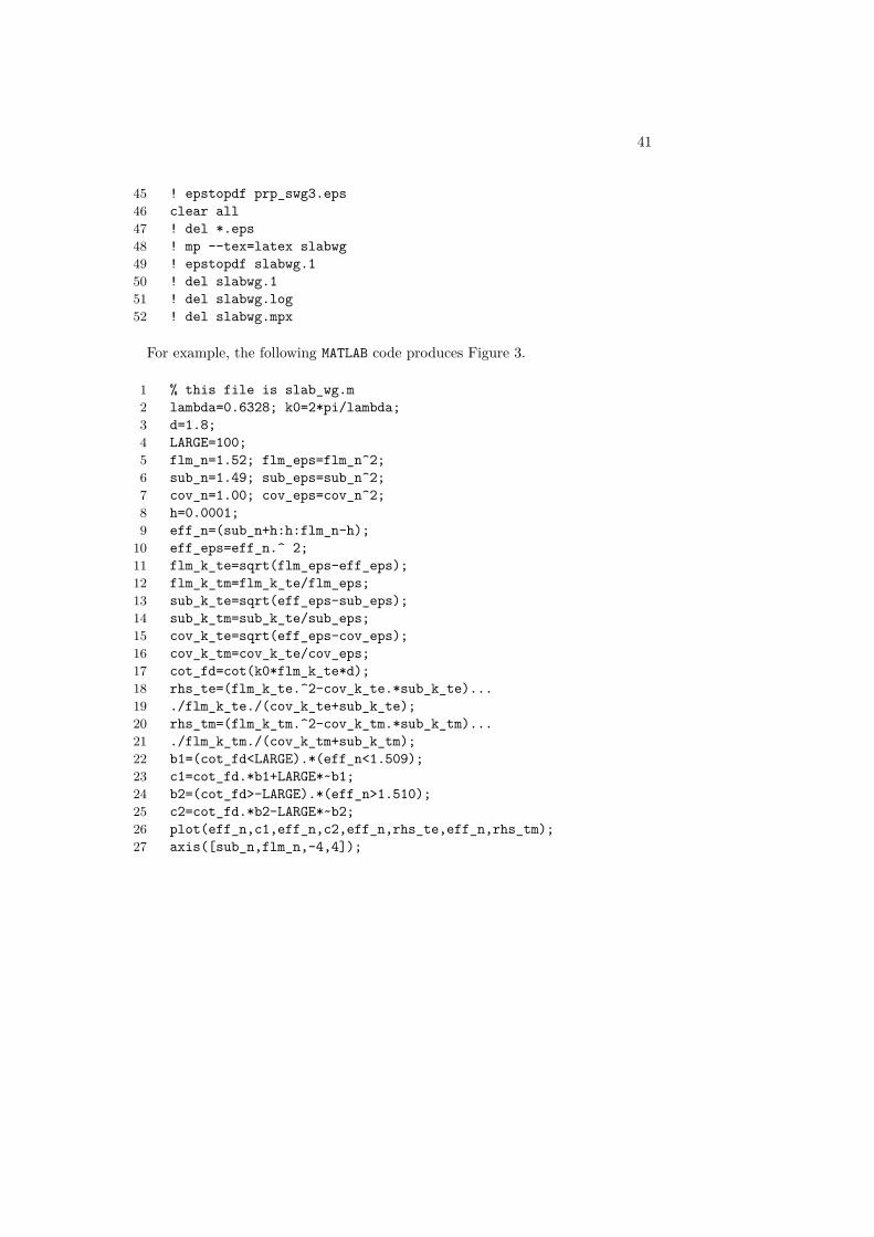
For example, the following MATLAB code produces Figure 3.

1 % this file is slab_wg.m2 lambda=0.6328; k0=2*pi/lambda;3 d=1.8;4 LARGE=100;5 flm_n=1.52; flm_eps=flm_n^2;6 sub_n=1.49; sub_eps=sub_n^2;7 cov_n=1.00; cov_eps=cov_n^2;8 h=0.0001;9 eff_n=(sub_n+h:h:flm_n-h);

10 eff_eps=eff_n.^ 2;11 flm_k_te=sqrt(flm_eps-eff_eps);12 flm_k_tm=flm_k_te/flm_eps;13 sub_k_te=sqrt(eff_eps-sub_eps);14 sub_k_tm=sub_k_te/sub_eps;15 cov_k_te=sqrt(eff_eps-cov_eps);16 cov_k_tm=cov_k_te/cov_eps;17 cot_fd=cot(k0*flm_k_te*d);18 rhs_te=(flm_k_te.^2-cov_k_te.*sub_k_te)...19 ./flm_k_te./(cov_k_te+sub_k_te);20 rhs_tm=(flm_k_tm.^2-cov_k_tm.*sub_k_tm)...21 ./flm_k_tm./(cov_k_tm+sub_k_tm);22 b1=(cot_fd<LARGE).*(eff_n<1.509);23 c1=cot_fd.*b1+LARGE*~b1;24 b2=(cot_fd>-LARGE).*(eff_n>1.510);25 c2=cot_fd.*b2-LARGE*~b2;26 plot(eff_n,c1,eff_n,c2,eff_n,rhs_te,eff_n,rhs_tm);27 axis([sub_n,flm_n,-4,4]);