did focusing on asia pacific emerging markets provide much...

Introduction

International openness to trade and capital flows have a potential to increase the vulner-ability of a country to international shocks. The recent international shock happened during the late 2000s when most securities suffered large losses erupted by the US subprime mortgage collapse in August 2007. It has resulted in a sharp drop in international trade, rising unem-ployment and slumping commodity prices and investments amount around the world. It also included a global explosion in prices, focused especially in commodities and housing, mark-ing an end to the commodities recession of

1980–2000. In 2008, the prices of many com-modities, notably oil and food, rose so high as to cause economic damage, threatening stag-flation and a reversal of globalization (Rubin, 2008). Some large financial institutions were collapsed and some national governments granted the bailout of the banks. The global re-cession also resulted in the downturns in stock markets around the world. On the international stock market, Standard & Poor in December 2009 reported that most countries in the S&P Indices experienced a serious negative impact on stock markets in 2008 as the effect of the global financial crisis took hold.

Did Focusing on Asia Pacific Emerging Markets Provide Much Benefit to Portfolio Diversification during the Late 2000s Recession?

Bambang Hermanto*Department of Management, Universitas Indonesia

Fajar Indra**Panin Sekuritas, alumni of Faculty of Economics Universitas Indonesia

This research studies the international co-movement among Asia Pacific emerging markets stock price indices during the late 2000s recession by using the monthly observations start from 1st Octo-ber 2001 until 1st April 2011. The co-integration analysis and parsimonious Vector Error Correction Model employed in this research reveal a long-term relationship and interdependencies among seven Asia Pacific emerging market stock price indices. This research finds that the unique co-integation exists on the equations. Specifically, two indices from China and Taiwan having meteor shower poten-tial while the rest indices from Thailand, Malaysia, and Indonesia are known to have heat waves ef-fects or country specific factors on the equation. Finally, all the results are linked to the international diversification strategies.

Keywords: Co-movement, co-integration, emerging market, heat waves, meteor shower, Asia Pacific, interdependencies, Vector Error Correction Model, international diversification

*Gedung Departemen Manajemen FEUI, Kampus Baru UI, Depok 16424, Indonesia, E-mail: [email protected] **Gedung Bursa Efek Indonesia Tower II, Suite 1705, Jl. Jend. Sudirman Kav. 52-53, Jakarta 12190, Indonesia, E-mail: [email protected]

1

Meanwhile, previous investigators found any interdependencies between some equity markets on crisis period since a high level of common short-run and long-run patterns of the market behavior tends to occur during the crisis. Forbes and Rigobon (2002) found any interde-pendencies during the 1997 Asian crisis, 1994 Mexican devaluation, and 1987 US market crash. They prefer to call it interdependencies since in their finding, co-movement does not increase significantly after the shocks. Baig and Goldfajn (1999) found a co-movement among financial markets of Thailand, Malaysia, Indo-nesia, Korea, and the Philippines. They found that correlations in currency increased signifi-cantly during the crisis period. Huyghebaert and Wang (2009) revealed that the relationships among East Asian stock markets were time var-ying. However, they revealed that there were integration and interdependencies among seven major East Asian stock exchanges before, dur-ing, and after the 1997–1998 Asian financial crises. Then, what about the latest 2000s reces-sion? Figure 1 depicts a structural break on all equity indices especially after the mid of 2008. The indices seemed to move together, declin-ing on the second semester of 2008, and then bouncing back one year after.

The typical co-movements and interdepend-encies on some crises suggest an unfavorable condition for creating some international port-folio diversifications. On the other side, pre-

vious investigators often stated that emerging markets are the best alternative solution for in-vesting in global economic crisis. Dattels and Miyajima (2009) stated that emerging markets are too worthy to miss because they have been relatively resilient to global market turmoil since they are able to avoid the kind of turbu-lence experienced in mature credit and other risk markets, especially in Asia. Emerging mar-ket returns typically have a low correlation with developed market returns (Errunza, 1983). The diversification potential of the emerging mar-kets is further supported by Harvey’s (1995) findings that the correlation between developed and emerging markets is less than 0.10. That implies that emerging countries’ equities may serve as attractive diversification vehicles for investors in developed countries.

This research seeks the internal relation-ship among Asia Pacific emerging market re-lationship during the late 2000s recession. The internal relationships may be revealed as co-movement or interdependencies. The investiga-tion is advanced by detecting the characteristics behind the transmission of the shocks, if any, based on Engle et al. (1990) hypothesis, “heat waves” and “meteor showers”. Finally, the im-plication of the interdependencies detected on this research is linked to the diversification pol-icy, especially for any equity investors around the globe.

INDONESIAN CAPITAL MARKET REVIEW • VOL.V • NO.1

2

Figure 1. Global stock market indices during the 2008 financial crisis

Literature Review

Optimum benefit of international diversifi-cation

The international portfolio activity will reach the optimum benefit when they are able to get the minimum risk. When the correlation coef-ficient between stock markets in one country of another are very low, it will imply that income portfolio that are balance-weighted greatly ben-efit from international diversification (Bodie et al., 2007). That is it, the basic technique for constructing the efficient international portfolio is still the efficient frontier. Markowitz (1952) has shown the main framework of the optimum mean-variance diversification in efficient fron-tiers concept. Portfolio risk depends on the cor-relation between the returns of the assets in the portfolio.

The variance of the portfolio is a sum of the contributions of the component security vari-ances plus a term that involves the correlation coefficient between the returns on the compo-nent securities. Therefore, Markowitz stated that a well-diversified portfolio means the port-folio with minimum variance so that the disper-sion of the expected returns will be minimized. For instance, once a portfolio is perfectly cor-related, it has a standard deviation which is a weighted-average of the standard deviation for each asset based on the weight of each asset in the portfolio. Thus, in this scenario investors do not obtain the risk reduction benefit from the diversification.

Co-movement

Baur (2004) once stated that there is no clear and unambiguous definition of term co-move-ment and no unique measure associated with it. It is also difficult to analyze in a time-varying context if it is based on the correlation coef-ficient. However, Barberis et al. (2005) deter-mined the explicit definition of co-movement as defined as a pattern of positive correlation. In general statistical usage, positive correlation means a correlation in which large values of one variable are associated with large values of

the other and small with small. Cahyadi (2009) described co-movement as co-integration, co-trending, and co-breaking. This definition was supported by Dolado et al. (1999) who stated that co-integration signifies co-movements among trending variables which could be ex-ploited to test for the existence of equilibrium relationships within a fully dynamic specifica-tion framework. Thus, this research concludes that the basic principle behind the term “co-movement” involves the common movements among any simultaneous variables during at certain time.

Furthermore, some common movement pat-terns have several distinctions when it comes to the characteristics affecting the movement. En-gle et al. (1990) proposed two hypotheses this characteristics. The first one is called the “heat wave” effect or country specific effect, a me-teorological analogy of a co-movement which is consistent with a view that major sources of disturbances are changes in country-specific fundamentals. In other words, it transmits the information internally within the same market on the previous t. The alternative hypothesis is “meteor shower” which rains down on the earth as it turns. The meteor shower effect transmits the information, as captured when they trade in different regions and time zones.

Previous empirical research

There are so many similar empirical re-searches that have been conducted to seek the interdependencies and international diversifica-tion among some stock market indices in any economic climate in the world. Azizan and Ah-mad (2008) revisited at the relationship between the movements of capital markets in developed economies and their emerging market counter-parts in the Asia Pacific region using market indices of the US, British, Malaysian, Singa-porean, Chinese, Hong Kong, Indian, Japanese, and Australian markets for the periods 1997 to 2007. They found several empirical results. The first one is the fact that the Asian markets are very much influenced by the events in the United States rather than other developed mar-kets. The second one is the fact that of all the

Hermanto and Indra

3

markets being surveyed, the South East Asian markets are the most sensitive towards events in their own regions outside themselves. Their last finding is the fact that Mainland China in the long-run is not affected by events outside themselves.

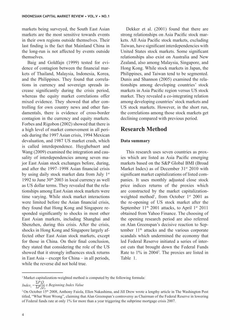
Baig and Goldfajn (1999) tested for evi-dence of contagion between the financial mar-kets of Thailand, Malaysia, Indonesia, Korea, and the Philippines. They found that correla-tions in currency and sovereign spreads in-crease significantly during the crisis period, whereas the equity market correlations offer mixed evidence. They showed that after con-trolling for own country news and other fun-damentals, there is evidence of cross-border contagion in the currency and equity markets. Forbes and Rigobon (2002) showed that there is a high level of market comovement in all peri-ods during the 1997 Asian crisis, 1994 Mexican devaluation, and 1987 US market crash, which is called interdependence. Huyghebaert and Wang (2009) examined the integration and cau-sality of interdependencies among seven ma-jor East Asian stock exchanges before, during, and after the 1997–1998 Asian financial crisis by using daily stock market data from July 1st 1992 to June 30th 2003 in local currency as well as US dollar terms. They revealed that the rela-tionships among East Asian stock markets were time varying. While stock market interactions were limited before the Asian financial crisis, they found that Hong Kong and Singapore re-sponded significantly to shocks in most other East Asian markets, including Shanghai and Shenzhen, during this crisis. After the crisis, shocks in Hong Kong and Singapore largely af-fected other East Asian stock markets, except for those in China. On their final conclusion, they stated that considering the role of the US showed that it strongly influences stock returns in East Asia – except for China – in all periods, while the reverse did not hold true.

Dekker et al. (2001) found that there are strong relationships on Asia Pacific stock mar-kets. All Asia Pacific stock markets, excluding Taiwan, have significant interdependencies with United States stock markets. Some significant relationships also exist on Australia and New Zealand, also among Malaysia, Singapore, and Hong Kong. While stock markets in Japan, the Philippines, and Taiwan tend to be segmented. Dunis and Shannon (2005) examined the rela-tionships among developing countries’ stock markets in Asia Pacific region versus US stock market. They revealed a co-integrating relation among developing countries’ stock markets and US stock markets. However, in the short run, the correlations among those stock markets get declining compared with previous period.

Research Method

Data summary

This research uses seven countries as prox-ies which are listed as Asia Pacific emerging markets based on the S&P Global BMI (Broad Market Index) as of December 31st 2010 with significant market capitalizations of listed com-panies. It uses monthly adjusted close stock price indices returns of the proxies which are constructed by the market capitalization-weighted method1, from October 1st 2001 as the re-opening of US stock market after the September 11th 2001 attacks, to April 1st 2011 obtained from Yahoo Finance. The choosing of the opening research period are also referred on Alan Greenspan’s decisive reaction to Sep-tember 11th attacks and the various corporate scandals which undermined the economy that led Federal Reserve initiated a series of inter-est cuts that brought down the Federal Funds Rate to 1% in 20042. The proxies are listed in Table_1.


4

1 Market capitalization-weighted method is computed by the following formula:

2 On October 15th 2008, Anthony Faiola, Ellen Nakashima, and Jill Drew wrote a lengthy article in The Washington Post titled, “What Went Wrong”, claiming that Alan Greenspan’s controversy as Chairman of the Federal Reserve in lowering of Federal funds rate at only 1% for more than a year triggering the subprime mortgage crisis 2007.

Table 2 shows the descriptive statistic among the proxies, compared with some devel-oped countries’ major indices relevant statis-tics. There are two important aspects informed by the table above. The first aspect is volatility. BSESN was the most volatile index among the group members and KLSE was the least volatile one during 2001 until 2010. The high monthly volatility, as a quadratic function of standard deviation, in BSESN, TWII, SSEC, JKSE, and PSEI implies that Asia Pacific emerging market is fairly volatile. The second aspect is the data distribution. The excess kurtosis in Asia Pacific emerging markets is significantly greater from zero. It indicates a fat-tailed distribution. The absolute skewness statistics are a bit greater than zero, revealing that the distributions are somewhat asymmetric.

The existance of the co-movement on Asia Pacific emerging markets indices can be rough-ly withdrawn by analyzing the pairwise correla-tion matrix on Table 3 above since most of the indices are strongly correlated to each other. The highest correlation coefficient implies to the re-

lationship between PSEI and KLSE in 0.9803. The lowest correlation coefficient implies to the relationship between SSEC and SETI in 0.051. The strong positive correlation coeficients in-dicates that most of variables are strongly co-moving on this decade. In other words, it can be said that the variables are strongly interde-pendent on each other. From this phenomenon, at glance investors do not obtain the risk reduc-tion benefit from the diversification. However, correlation matrix does not show the dynamic and simultaneous relationship among the vari-ables since it can not ensure the integration and interdependencies among the variables (Cahy-adi, 2009).

Co-integration analysis

This research describes co-integration as a set of variables with a stationary linear combi-nation of them (Engle and Granger, 1987). The co-integration test shall be conducted to seek if there is any long-term relationship or equilib-rium among the Asia Pacific emerging markets’

Hermanto and Indra

5

Table 1. List of major indices on Asia Pacific emerging marketsIndex Ticker Country Index Ticker Country

Jakarta Composite Index JKSE Indonesia Kuala Lumpur Composite Index KLSE MalaysiaShanghai Stock Exchange Composite Index SSEC China Philippines Stock Exchange Index PSEI Philippines

Bombay Stock Exchange Sensex BSESN India Taiwan Stock Exchange Index TWII TaiwanStock Exchange of Thailand Index SETI Thailand

Source: S&P Global BMI (Broad Market Index) as of December 31st 2010

Table 2. Descriptive statistic of Asia Pacific emerging market stock price indices BSESN JKSE KLSE PSEI SETI SSEC TWII

Mean 10541.4 1565.6 1016.1 2305.9 651.44 2241.9 6610.3 Std. Dev. 5711.20 964.90 267.93 920.5 186.52 1077.9 1413.1 Skewness 0.1408 0.5547 0.3776 0.3339 -0.1272 1.2957 0.1313 Kurtosis 1.5941 2.2173 1.9177 1.9868 2.551 4.3384 2.1629 Obs. 115 115 115 115 115 115 115

Source: Author's own calculation

Table 3. Pairwise correlation matrix of Asia Pacific emerging market stock price indicesCorrelation BSESN PSEI SSEC TWII SETI KLSE JKSE

BSESN 1.000000PSEI 0.963047 1.000000SSEC 0.771458 0.751814 1.000000TWII 0.866697 0.900711 0.766250 1.000000SETI 0.798446 0.843705 0.505131 0.863948 1.000000KLSE 0.961676 0.980311 0.783464 0.915473 0.851562 1.000000JKSE 0.971072 0.959831 0.713310 0.840366 0.814037 0.971260 1.000000


stock price indices. The test of co-integration is conducted by the Johansen’s test as the using of multivariate system, begins with defining a vector Zt of n potentially endogenous variables following Johansen (1988) and Harris (2003). Zt is assumed as an unrestricted VAR system in k-lags:

Zt=A1Zt-1+A2Zt-2... ... ... +AkZt-k+ΦDt+μ+εt 1)

where Zt is n x 1 and A1 is n x n matrix of pa-rameters, μ is a constant, Dt is a dummy vari-able that is orthogonal with μ constant, and er-ror εt is assumed to be independent. This way estimates dynamic relationships among jointly endogenous variables without imposing strong a priori restrictions (Harris, 2003). The equa-tion (1) can be reformulated into Vector Error Correction Model (VECM) by subtracting Zt-1 of the both equation sides:

ΔZt=Γ1ΔZt-1+...+Γk-1ΔZt-k+1+ΠZt-k+ΦDt+μ+ut 2)

where Γi = - (I - A1 -…- Ai), (i = 1, …, k-1), and Π = - (I - A1 - … - Ak).

Equation (2) contains some information on both short term and long term error correction models to ΔZt, via the estimates of Γ and Π re-spectively. As will be seen, Π = αβ’, where α represents the speed of adjustment to disequi-librium and β is a matrix of long-run coeffi-cients such that the term β’Zt-k embedded in equation (2) represents up to (n - 1) co-inte-gration relationships in the multivariate model which ensure that the Zt converge to their long-run steady-state solutions.

Assuming Zt is a vector non-stationary I(1) variables, then the term (2) which involve ΔZt are I(0) while ΠZt-k must also be stationary for ut ~ I(0) to be white noise. There are three instanc-es when this requirement ΠZt-k ~ I(0) is met: 1. If Π has full rank or there are r = n linearly

independent columns, then all variables will be stationary on level. It implies that there is no problem of spurious regression and the appropriate modeling strategy is to estimate the standard VAR in levels.

2. If the rank of Π is zero, then it will imply that there are no linear combinations of the Zt that are I(0), and consequently Π is an (n x n) matrix of zeros. In this case the appropriate model is a VAR in first differences involving no long-run elements.

3. The third instance is when Π has reduced rank, then there will exist up to (n – 1) co-integration relationships: β’Zt-k ~ I(0). In this instance r ≤ (n - 1) co-integration vector ex-ists in β, together with (n - r) non-stationary vectors. Only the co-integration vectors in β enter (equation 3), otherwise ΠZt-k would not be I(0), which implies that the last (n – r) col-umns of α are insignificantly small. In this case the appropriate model is a VECM. To test the null hypothesis that there are at

most r co-integration vectors can be used what has become known as trace statistic:

λtrace = -2log(Q) = -T log(1- ) 3)

r = 0,1,2, ... , (-2), (-1)

where Q is the ratio between restricted maxi-mized likelihood between unrestricted maxi-mized likelihood. Besides that, another test of the significant of the largest λ is the so-called maximal Eigenvalue or λmax statistic, formulat-ed as follows: λmax = -T log(1- ) 4)

r = 0,1,2, ... , (n-2), (n-1)

The maximum-Eigenvalue tests that there are r co-integration vectors againts the alterna-tive that (r + 1) exist.

Vector Autoregression (VAR)

In a Vector Autoregression (VAR) model the current value of each variable is a linear func-tion of the past values of all variables plus ran-dom disturbances. All the variables in a VAR are treated symmetrically by including for each variable an equation explaining its evolution based on its own lags and the lags of all the other variables in the model. Suppose that each


6

equation contains k lag values of Y and X. In this case, one can estimate each of the follow-ing equations by OLS:

5)

6)

where the u is the stochastic error term, called impulse or innovation or shock or white noise disturbance term.

Unrestricted VAR

This type of VAR illustrates the value of VAR as a linear function of its value on the past. The value on the past of other variables is the serially uncorrelated error term. This type of VAR can be divided into VAR on level and VAR on first difference. The unrestricted VAR on level is used for stationary data or if Π has full rank or there are r = n linearly independ-ent columns. Whereas, the unrestricted VAR on first difference shall be used if the rank of Π is zero or if there are no linear combinations of the Zt that are I(0)

Vector Error Correction Model

The model becomes a Vector Error Cor-rection Model (VECM) which can be seen as a restricted VAR. This type of VAR restricts the long-term relationship of the endogenous variables so that there are convergent co-inte-grations but still tolerance the short-term dy-namics. This type of VAR is used for data that has reduced rank on its Π or there exist up to (n – 1) co-integration relationships. When the variables are co-integrated, the error correction term has to be included in the VAR. The co-in-tegration term is also known as an “error” since the deviation of the long-term equilibrium is corrected gradually through the partial series of short term adjustments. Recalling the bivariate version of VAR equations (5) and (6), Zt value on VAR(2) can be decomposed as follows:

7)

where can be reformulated into Vector Error Correction Model (VECM) by subtracting Zt-1 of the both equation sides:

8)

where: Π = -(I-Φ1-Φ2) = -Φ(1) and Γ = -(Φ1+Φ2) = -(I-Φ1)

From the decomposition above, the VECM model can be reformulated as detail estimation:

9)

As described previously, the rank Π equals to αβ’, where α represents the speed of adjust-ment to disequilibrium and β is a matrix of long-run coefficients. If the rank Π is k, then α can be decomposed as k x 2 matrix while β is decomposed as 2 x k matrix on the bivariate VECM. Therefore, the error correction term of the equation (9) is determined follow:

10)

Granger Causality test

The causality testing can figure out whether an endogenous variables can be treated as an ex-ogenous one. The causality relationship can be tested by Granger Causality test with assump-tion that the information relevant to the predic-tion of the respective variables. The Granger Causality test is a statistical hypothesis test for determining whether one time series is useful in forecasting another (Granger, 1969). However, bivariate Granger Causality is not sufficient to imply true causality in multivariate system. A similar test involving more variables can be ap-

Hermanto and Indra

7

plied with Vector Autoregression (VAR). On an examination process of VAR model, it needs to conduct simultaneously so that there will be a combined significances on the equation (Ham-ilton, 1994; Patterson, 2000). All VAR estima-tions shall be tested on Wald Chi-squares dis-tribution (χ2-Wald). The statistical results of χ2-Wald shall show the joint significance of the endogenous variables on VAR estimation.

Is this test always valid for every measure-ment? Toda and Phillips (1993) stated that the empirical use of Granger Causality tests in levels VAR is not to be encouraged in general when there are stochastic trends and the possi-bility of co-integration3. That is, causality tests are valid asymptotically as χ2-Wald criteria only when there is sufficient co-integration with re-spect to the variables whose causal effects are being tested. Since the estimates of such ma-trices in levels VAR suffers from simultaneous equations bias there is no valid statistical basis for determining whether the required sufficient condition applies.

Impulse Response Function

In structural analysis, certain assumptions about the causal structure of the data under in-vestigation are imposed, and the resulting caus-al impacts of unexpected shocks or innovations to the specific variables on the variables in the model are summarized. These causal impacts are usually summarized with impulse response functions and forecast error variance decompo-sitions.

This research emphasizes on Impulse Re-sponse Function (IRF) as a tool on VAR anal-ysis to see the response and the future effects to the shocks or changes in other variables in the VAR system. An impulse response function traces out the response of a variable of inter-est to an exogenous shock. The shocks and in-novations of each variable are correlated each other so that those variables have the same component but are unable to be specifically at-tributed to a certain variable. This problem can

be overcome by creating the orthogonal error using Cholesky decomposition method. The mathematical approach of the IRF is conducted by manipulating the VAR equations on (5) and (6) into the matrices below:

11)

From the equation above, it is obvious that the value of Y and X depend on their respective lag and residual values. By focusing the deriva-tion into the influence of residual shock chang-ing ε1t and ε2t on the value of Y and X, the equa-tion (11) can be denoted as follows:

12)

Those φ11, φ21, φ12, and φ22 are the im-pulse response function coefficient.

Result and Discussion

Co-integration analysis

This research has found that all indices are stationary in first difference I(1). Thus, if there is no co-integration found on the system, the first difference VAR will be able to be con-ducted. This research conducts the optimum lag based on the least result of Final Prediction Error, which is lag 1. The optimum lag length declaration must be done before estimating the models since the simultaneous equation process such as VAR and co-integration test is very sen-sitive to the lag length (Enders 2004). Based on the optimum lag declared, the Johansen’s co-integration test is conducted.

To determine the appropriate assumption of the Johansen’s co-integration test, five sets of assumptions that stated that the co-integration test should be conducted with intercept and trend assumption on CE with linear determin-istic trend in data. Dummy variable is set for


8

3 They developed a limit theory for Wald tests of Granger Causality in levels Vector Autoregressions (VAR) and Johansen-type error correction models (ECM), allowing for the presence of stochastic trends and co-integration. For further expla-nation, see Toda and Phillips (1993).

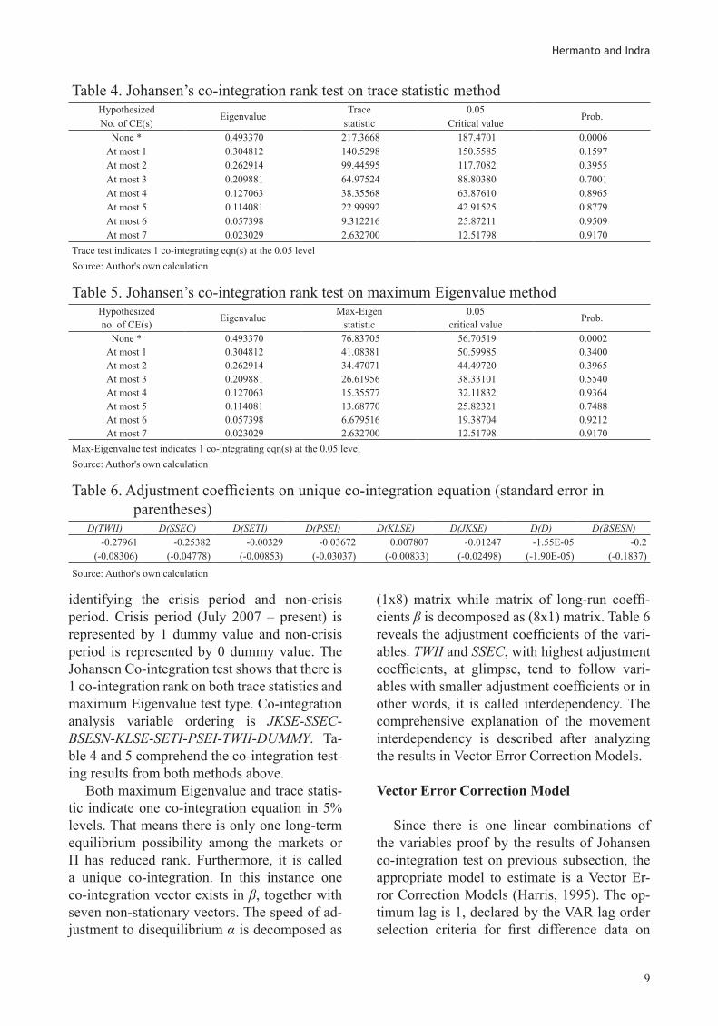
identifying the crisis period and non-crisis period. Crisis period (July 2007 – present) is represented by 1 dummy value and non-crisis period is represented by 0 dummy value. The Johansen Co-integration test shows that there is 1 co-integration rank on both trace statistics and maximum Eigenvalue test type. Co-integration analysis variable ordering is JKSE-SSEC-BSESN-KLSE-SETI-PSEI-TWII-DUMMY. Ta-ble 4 and 5 comprehend the co-integration test-ing results from both methods above.

Both maximum Eigenvalue and trace statis-tic indicate one co-integration equation in 5% levels. That means there is only one long-term equilibrium possibility among the markets or Π has reduced rank. Furthermore, it is called a unique co-integration. In this instance one co-integration vector exists in β, together with seven non-stationary vectors. The speed of ad-justment to disequilibrium α is decomposed as

(1x8) matrix while matrix of long-run coeffi-cients β is decomposed as (8x1) matrix. Table 6 reveals the adjustment coefficients of the vari-ables. TWII and SSEC, with highest adjustment coefficients, at glimpse, tend to follow vari-ables with smaller adjustment coefficients or in other words, it is called interdependency. The comprehensive explanation of the movement interdependency is described after analyzing the results in Vector Error Correction Models.

Vector Error Correction Model

Since there is one linear combinations of the variables proof by the results of Johansen co-integration test on previous subsection, the appropriate model to estimate is a Vector Er-ror Correction Models (Harris, 1995). The op-timum lag is 1, declared by the VAR lag order selection criteria for first difference data on

Hermanto and Indra

9

Table 4. Johansen’s co-integration rank test on trace statistic methodHypothesized

EigenvalueTrace 0.05

Prob.No. of CE(s) statistic Critical value

None * 0.493370 217.3668 187.4701 0.0006At most 1 0.304812 140.5298 150.5585 0.1597At most 2 0.262914 99.44595 117.7082 0.3955At most 3 0.209881 64.97524 88.80380 0.7001At most 4 0.127063 38.35568 63.87610 0.8965At most 5 0.114081 22.99992 42.91525 0.8779At most 6 0.057398 9.312216 25.87211 0.9509At most 7 0.023029 2.632700 12.51798 0.9170

Trace test indicates 1 co-integrating eqn(s) at the 0.05 levelSource: Author's own calculation

Table 5. Johansen’s co-integration rank test on maximum Eigenvalue methodHypothesized Eigenvalue Max-Eigen 0.05 Prob.no. of CE(s) statistic critical value

None * 0.493370 76.83705 56.70519 0.0002At most 1 0.304812 41.08381 50.59985 0.3400At most 2 0.262914 34.47071 44.49720 0.3965At most 3 0.209881 26.61956 38.33101 0.5540At most 4 0.127063 15.35577 32.11832 0.9364At most 5 0.114081 13.68770 25.82321 0.7488At most 6 0.057398 6.679516 19.38704 0.9212At most 7 0.023029 2.632700 12.51798 0.9170

Max-Eigenvalue test indicates 1 co-integrating eqn(s) at the 0.05 levelSource: Author's own calculation

Table 6. Adjustment coefficients on unique co-integration equation (standard error in parentheses)

D(TWII) D(SSEC) D(SETI) D(PSEI) D(KLSE) D(JKSE) D(D) D(BSESN)-0.27961 -0.25382 -0.00329 -0.03672 0.007807 -0.01247 -1.55E-05 -0.2

(-0.08306) (-0.04778) (-0.00853) (-0.03037) (-0.00833) (-0.02498) (-1.90E-05) (-0.1837)


previous subsection. The equation is conducted with intercept and trend assumption on CE with linear deterministic trend in data.

The comprehensive VECM estimates for seven Asia Pacific emerging market indices are listed in table 7. The numbers within the parentheses describes the t-statistics value. The F tests given in that table are to test the hypothesis that collectively the various lagged coefficients are zero. The high F-stat value on SSEC and TWII equations reveals the “meteor shower” potential on those variables. However, the statistically least significant lag variables are sequentially eliminated so that parsimoni-ous specification is obtained following Ndako (2008). The parsimonious VECM is used to ex-amine the existence of significant interdepend-encies among variables.

The VECM equations suggest that there ex-ists an interdependence pattern in response to SSEC. The significant influences come from the response of JKSE, BSESN, and PSEI so that the parsimonious equation is built using those variables as independent ones. The estimation is conducted on first difference data. Table 8 shows the results of parsimonious VECM with SSEC as dependent variable.

The “meteor shower” effect apparently ex-ists on the internal relationship effects on SSEC. With R-squared 0.675 and F-stat coef-ficient 57.056, the parsimonious VECM sug-gests that SSEC is significantly influenced by JKSE on the previous lag, BSESN on the previ-ous lag, and PSEI on the previous lag. It can be said that the main factors that influenced the SSEC movement pattern are BSESN, JKSE, and


10

Table 7. Vector Error Correction Model estimatesError Correction: D(JKSE) D(SSEC) D(BSESN) D(KLSE) D(SETI) D(PSEI) D(TWII) D(D)

CointEq1 -0.0187 -0.3802 -0.2996 0.01169 -0.0049 -0.0550 -0.4188 -2.3E-05[-0.4992] [-5.3123] [-1.0887] [ 0.9369] [-0.3857] [-1.2092] [-3.3665] [-0.8036]

D(JKSE(-1)) 0.19238 0.72303 1.935604 0.13864 0.12521 0.114708 0.767379 9.44E-05

[ 1.1310] [ 2.2228] [ 1.5476] [ 2.4440] [ 2.1557] [ 0.5548] [ 1.3571] [ 0.7177]D(SSEC(-1)) -0.04004 -0.13183 -0.41211 -0.00779 -0.00154 -0.07617 -0.09229 1.20E-05

[-0.7668] [-1.3202] [-1.0734] [-0.4473] [-0.0865] [-1.2002] [-0.5317] [ 0.2984]D(BSES(-1)) -0.04111 -0.18189 -0.39013 -0.01231 -0.01451 -0.04341 -0.28373 -2.7E-05

[-1.6663] [-3.8546] [-2.1503] [-1.4962] [-1.7229] [-1.4472] [-3.4589] [-1.4033]D(KLSE(-1)) 0.495301 -0.47180 3.328057 0.09186 0.03936 0.858592 0.329165 -0.00013

[ 1.1358] [-0.5657] [ 1.0380] [ 0.6316] [ 0.2643] [ 1.6199] [ 0.2271] [-0.3974]D(SETI(-1)) 0.114274 -0.50190 1.523858 -0.03109 -0.02413 0.343491 1.513761 -6.2E-05

[ 0.2823] [-0.6485] [ 0.5121] [-0.2303] [-0.1746] [ 0.6983] [ 1.1252] [-0.1985]D(PSEI(-1)) 0.13918 0.761293 1.206895 0.02353 0.01177 -0.02985 0.6473 6.39E-05

[ 1.2120] [ 3.4666] [ 1.4293] [ 0.6143] [ 0.3002] [-0.2138] [ 1.6956] [ 0.7191]D(TWII(-1)) 0.00095 0.103464 -0.05415 0.00197 0.01037 0.042958 0.180185 1.68E-05

[ 0.0244] [ 1.3919] [-0.1895] [ 0.1524] [ 0.7818] [ 0.9092] [ 1.3945] [ 0.5596]D(D (-1)) -99.8649 -347.771 -932.312 -66.7648 -21.9059 -126.797 -414.296 -0.03997

[-0.7618] [-1.3873] [-0.9673] [-1.5272] [-0.4894] [-0.7958] [-0.9507] [-0.3943]C -20.3597 2.791016 -72.8366 -4.30451 -4.18908 -19.4120 -20.2838 0.009098

[-1.6596] [ 0.1190] [-0.8075] [-1.0521] [-1.0000] [-1.3018] [-0.4974] [ 0.9591] R-squared 0.091441 0.294196 0.121806 0.14602 0.08478 0.09706 0.171817 0.023102 F-statistic 1.151818 4.770323 1.587349 1.95686 1.06025 1.230195 2.374302 0.270639


Table 8. Parsimonious VECM with DSSEC as dependent variableVariable Coefficient Std. error t-Statistic Prob.

DJKSE -1.415195 0.304771 -4.643464 0.0000DPSEI 0.360639 0.257165 5.402362 0.1636DBSESN 0.400682 0.066115 6.060332 0.0000C -1024.478 392.3037 -2.611441 0.0103R-squared 0.674763 F-statistic 57.05365


PSEI. However, to say that it consists of meteor shower effects, the exogeneity test should be conducted since that effect examines the cau-sality relationship among variables.

The VECM equations also suggest that an interdependence pattern exists in response to TWII. Only that the significant influences come only from the response of BSESN. The parsimo-nious VECM again prove that the relationship between TWII and BSESN significantly exists. At last, the VECM equation suggests that JKSE and PSEI are not significantly influenced by other proxies. The tendency of the heat waves effect seems existing on these situations though the situations on JKSE and PSEI are inconclu-sive. The causality relationship to examine the direction of causality is tested by Multivariate Granger Causality test based on the output of parsimonious VECM test.

Granger Causality test

Toda and Phillips (1993) stated that the cau-sality tests are valid asymptotically as χ2-Wald

criteria only when there is sufficient co-integra-tion with respect to the variables whose causal effects are being tested. Since the data have one co-integration relationship, the Granger Cau-sality test can be used to detect the specific cau-sality relationship among variables. The greater χ2-Wald value suggests the endogenous vari-able significantly cause the exogenous variable.

The empirical of the Pairwise Granger Cau-sality suggests that BSESN Granger causes SSEC (χ2 = 14.85839), PSEI Granger causes SSEC (χ2 = 12.01752), and BSESN Granger causes TWII (χ2 = 11.96404). Eight bivariate causality relationships that are found on those variables strengthen the co-integration pattern among the variables.

From those types of Granger Causality test, the results can be summarized into the causal-ity relationship Figure 2. It depicts that in the system, the major sources of disturbances are changes in country-specific fundamentals, espe-cially in PSEI, BSESN, SETI, KLSE, and JKSE. In other words, it transmits the information in-ternally within the same market and tend to suf-

Hermanto and Indra

11

Table 9. Parsimonious VECM with DTWII as dependent variableVariable Coefficient Std. Error t-Statistic Prob.

DBSESN 0.214449 0.011611 18.46923 0.0000C 4349.748 139.0694 31.27753 0.0000R-squared 0.751163 F-statistic 341.1123


Figure 2. The causality relationship on Asia Pacific emerging market stock price indices

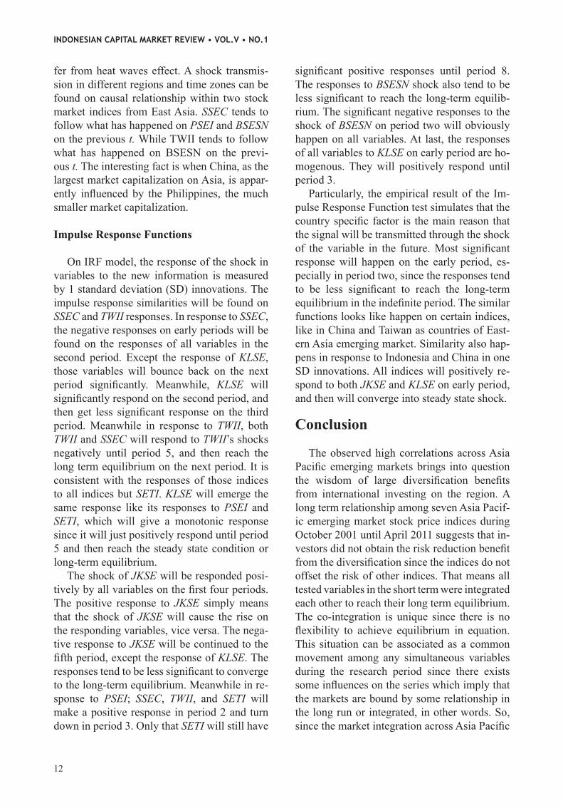
fer from heat waves effect. A shock transmis-sion in different regions and time zones can be found on causal relationship within two stock market indices from East Asia. SSEC tends to follow what has happened on PSEI and BSESN on the previous t. While TWII tends to follow what has happened on BSESN on the previ-ous t. The interesting fact is when China, as the largest market capitalization on Asia, is appar-ently influenced by the Philippines, the much smaller market capitalization.

Impulse Response Functions

On IRF model, the response of the shock in variables to the new information is measured by 1 standard deviation (SD) innovations. The impulse response similarities will be found on SSEC and TWII responses. In response to SSEC, the negative responses on early periods will be found on the responses of all variables in the second period. Except the response of KLSE, those variables will bounce back on the next period significantly. Meanwhile, KLSE will significantly respond on the second period, and then get less significant response on the third period. Meanwhile in response to TWII, both TWII and SSEC will respond to TWII’s shocks negatively until period 5, and then reach the long term equilibrium on the next period. It is consistent with the responses of those indices to all indices but SETI. KLSE will emerge the same response like its responses to PSEI and SETI, which will give a monotonic response since it will just positively respond until period 5 and then reach the steady state condition or long-term equilibrium.

The shock of JKSE will be responded posi-tively by all variables on the first four periods. The positive response to JKSE simply means that the shock of JKSE will cause the rise on the responding variables, vice versa. The nega-tive response to JKSE will be continued to the fifth period, except the response of KLSE. The responses tend to be less significant to converge to the long-term equilibrium. Meanwhile in re-sponse to PSEI; SSEC, TWII, and SETI will make a positive response in period 2 and turn down in period 3. Only that SETI will still have

significant positive responses until period 8. The responses to BSESN shock also tend to be less significant to reach the long-term equilib-rium. The significant negative responses to the shock of BSESN on period two will obviously happen on all variables. At last, the responses of all variables to KLSE on early period are ho-mogenous. They will positively respond until period 3.

Particularly, the empirical result of the Im-pulse Response Function test simulates that the country specific factor is the main reason that the signal will be transmitted through the shock of the variable in the future. Most significant response will happen on the early period, es-pecially in period two, since the responses tend to be less significant to reach the long-term equilibrium in the indefinite period. The similar functions looks like happen on certain indices, like in China and Taiwan as countries of East-ern Asia emerging market. Similarity also hap-pens in response to Indonesia and China in one SD innovations. All indices will positively re-spond to both JKSE and KLSE on early period, and then will converge into steady state shock.

Conclusion

The observed high correlations across Asia Pacific emerging markets brings into question the wisdom of large diversification benefits from international investing on the region. A long term relationship among seven Asia Pacif-ic emerging market stock price indices during October 2001 until April 2011 suggests that in-vestors did not obtain the risk reduction benefit from the diversification since the indices do not offset the risk of other indices. That means all tested variables in the short term were integrated each other to reach their long term equilibrium. The co-integration is unique since there is no flexibility to achieve equilibrium in equation. This situation can be associated as a common movement among any simultaneous variables during the research period since there exists some influences on the series which imply that the markets are bound by some relationship in the long run or integrated, in other words. So, since the market integration across Asia Pacific


12

emerging market exists, it can be said that fo-cusing on Asia Pacific emerging markets did not provide much benefit to international diver-sification during the late-2000s recession. Fo-cusing the portfolio on the Asia Pacific emerg-ing market only is not encouraged considering the final result of the research. Equity investors, need to hedge the risk of the portfolio by diver-sifying their assets on may be different emerg-ing market region on the globe, such as Mid-west, Africa, Europe, or South America.

Several interdependencies on the multivari-ate systems are revealed by parsimonious Vec-tor Error Correction Model. The estimations of SSEC and TWII, which belong to East Asian hemisphere, are the most significant estimates among the others. They tend to follow certain variables from the previous time (t – 1). The multivariate Granger Causality tests strengthen the phenomenon that SSEC and TWII have me-teor shower potential. Meanwhile, the rest vari-ables such as KLSE, SETI, and JKSE tend to have heat waves effects since they are not sig-nificantly influenced by other variables in mul-tivariate system. The result is consistent with Engle et al. (1990) statement that the “meteor showers” and “heat waves” effects are not mu-tually exclusive and, hence, during any period of time both of them can co-exist, even though one may dominate. The Impulse Response

Function simulates that the country specific factor is the main reason that the signal will be transmitted through the shock of the variable in the future. Most significant response will hap-pen on the early period then the responses tend to be less significant to reach the long-term equilibrium in the indefinite period.

For the next research, the analysis and find-ing of volatility spillovers during the crisis is encouraged since the stock movement may vary over time. The volatility analysis provides more information of the variables’ interdepend-encies and information transmissions and is very useful in detecting the existence of time-varying variance and volatility clustering on the observed data. When return distribution data shows asymmetric pattern, and the associated variances are non constant, the resulting model can be used to predict (Febrian and Herwany, 2009). Since this research employs only 114 monthly data during the global financial crisis 2008, the detail estimations on the pre -crisis and on-crisis period are not possible to estimate. The monthly data is al so not encouraged to es-timate the variance process since the standard deviations of the data will be so high (Engle et al., 1990). That is the reason that this research does not touch the variance process estimation to determine the volatility spillovers.

Hermanto and Indra

13

ReferencesAzizan, N.A. and Ahmad, Z. (2008), The Rela-

tionship Between The Movements of Capital Markets in Developed Economies and Their Emerging Market Couterparts in Asia Pa-cific Region, Indonesian Capital Market Re-view, 8(2), 103-115.

Baig, T. and Goldfajn, I. (1999), Financial Market Contagion in the Asian Crisis, IMF Staff 46(2), 167-195.

Barberis, N., Shleifer, A., and Wurgler, J. (2005), Comovement, Journal of Financial Economics, 75, 283-317.

Baur, D. (2004), What Is Comovement?, Wor-king Paper, European Commission, Joint Research Center, Ispra (VA), Italy.

Bodie, Z., Kane, A., and Marcus, A.J. (2007), Essentials of Investments 6th Ed., Singapore: McGraw-Hill.

Brooks, C. (2008), Introductory Econometric for Finance 2nd Ed., Cambridge: Cambridge University Press.

Brown, K. and Reilly, F. (2005), Investment Analysis and Portfolio Management 7th Ed., New York: McGraw-Hill.

Cahyadi, K. (2009), Comovement Imbal Hasil Indeks – Indeks Sektoral Indonesia Peri-ode Bearish dan Bullish Antara Tahun 1999 Hingga 2008 dan Implikasinya Pada Di-vesifikasi Portofolio, Unpublished, Fakultas Ekonomi Universitas Indonesia.


14

Conover, C.M., Jensen, G.R., and Johnson, R.R. (2002), Emerging Markets: When Are They Worth It?, Financial Analysts Journal, 58(2), 86-95.

Dattels, P. and Miyajima, K. (2009), Will Emerging Markets Remain Resilient to Global Stress?, Global Journal of Emerging Market Economies, 1(1), 5-24.

Dekker, A., Sen, K., and Martin, R.Y. (2001), Equity Market Linkages in the Asia Pacific Region: A Comparison of the Orthogonal-ised and Generalised VAR Approaches, Global Finance Journal, 12, 1-33.

Driessen, J. and Laeven, L. (2007), Internation-al Portfolio Diversification Benefits: Cross-Country Evidence from a Local Perspective, Working Paper, World Bank.

Dolado, J. J., Gonzalo, J., and Marmol, F. (1999), Co-integration, Working Paper, Uni-versidad Carlos III de Madrid, Spain.

Dunis, C.L. and Shannon, G. (2005), Emerging Markets of South-East and Central Asia: Do They Still Offer a Diversification Benefit?, Journal of Asset Management; 6(3), 168.

Enders, W. (2004), Applied Econometric Time Series 2nd Ed., New York: John Wiley and Sons, Inc.

Engle, R.F., Ito, T., and Lin, W.L. (1990), Me-teor Showers or Heat Waves? Heteroske-dastic Intra-Daily Volatility in the Foreign Exchange Market, Econometrica, 58(3), 525-542.

Engle, R.F. and Granger, C.W.J. (1987), Co-in-tegration and Error Correction: Representa-tion, Estimation, and Testing, Econometrica, 55, 251-76

Errunza, V. (1983), Emerging Markets: A New Opportunity for Improving Global Portfolio Performance, Financial Analyst Journal, 39, 51-58.

Ferbian, E. and Herwany, A. (2009), Volatility Forecasting Models and Market Co-integra-tion: A Study on South-East Asian Markets, Journal of Indonesian Capital Market Re-view, 1, 27-42.

Forbes, K. J. and Rigobon, R. (2002), No Con-

tagion, Only Interdependence: Measuring Stock Market Comovements, The Journal of Finance, 57(5), 2223-2261.

Grubel, H.G. (1968), Internationally Diversi-fied Portfolios: Welfare Gains and Capital Flows, American Economic Review, 58, 1299-1314.

Gujarati, D.N. (2003), Basic Econometric 4th Ed., New York: McGraw Hill.

Harris, R. (1995), Using Cointegration Analy-sis in Econometric Modelling, Hemel Hamp-stead: Prentice Hall.

Harvey, C.R. (1995), Predictable Risk and Re-turns in Emerging Markets, Review of Fi-nancial Studies, 8, 773-816.

Hjalmarsson, E. and Österholm, P. (2007), Test-ing for Cointegration Using the Johansen Methodology when Variables are Near-In-tegrated, International Finance Discussion Papers, 915.

Huyghebaert, N. and Wang, L. (2010), The Co-movement of Stock Markets in East Asia: Did the 1997–1998 Asian Financial Crisis Really Strengthen Stock Market Integra-tion?, China Economic Review, 21, 98–112.

Johansen, S. (1988), Statistical Analysis of Co-integration Vectors, Journal of Economic Dynamics and Control, 12, 231-254.

Markowitz, H.M. (1952), Portfolio Selection, Journal of Finance, 7, 77-91.

Ndako, U.B. (2008), Stock Markets, Banks and Economic Growth: A Time-Series Evidence from South Africa, Working Paper, Depart-ment of Economics University of Leicester, United Kingdom.

Rubin, J. (2008), The New Inflation (PDF), StrategEcon (CIBC World Markets), Re-trieved 2011-01-06.

Toda, H.Y. and Phillips, P.C.B. (1993), Vector Autoregressions and Causality, Economet-rica, 61(6), 1367-1393

Wassell, C.S. and Saunders, P.J. (2000), Time Series Evidence on Social Security and Pri-vate Saving: The Issue Revisited, Depart-ment of Economics, Central Washington University.

did focusing on asia pacific emerging markets provide much...

Documents