developing video measurement of strain for

DEVELOPING VIDEO MEASUREMENT OF STRAIN FOR

POLYMERS USING LABVIEW

By

MAZHARUL ISLAM

Bachelor of Science in Mechanical EngineeringBangladesh University of Engineering & Technology

(BUET)Dhaka, Bangladesh

2008

Submitted to the Faculty of theGraduate College of

Oklahoma State Universityin partial fulfillment ofthe requirements for

the Degree ofMASTER OF SCIENCE

May, 2011

COPYRIGHT c©

By

MAZHARUL ISLAM

May, 2011

DEVELOPING VIDEO MEASUREMENT OF STRAIN FOR

POLYMERS USING LABVIEW

Thesis Approved:

Dr. Jay C. Hanan

Thesis Advisor

Dr. Ranji Vaidyanathan

Dr. Prabhakar Pagilla

Dr. Mark E. Payton

Dean of the Graduate College

iii

ACKNOWLEDGMENTS

First and the foremost, I am heartily thankful to my supervisor, Dr. Jay C.

Hanan, whose encouragement, guidance and support from the initial to the final

level enabled me to develop an understanding of the subject and without which this

work would not have been possible. He taught me how to think in a different way

when I face a riddle. Every time when I felt in a situation where I could not find

the solution, his valuable advice makes me overcome all my difficulty. I am grate-

ful for his support and patience throughout my studies in Oklahoma State University.

I owe my deepest gratitude to the members of my advisory committee, Dr. Prab-

hakar R. Pagilla and Dr. Ranji Vaidyanathan for finding time in their busy schedule.

I would like to thank Dr. Raman P. Singh for his helpful contribution of ideas when-

ever needed.

I am also indebted to my many of my colleagues to support me for helping me to

understand the different subjects. I would like to thank Sudheer Badla for teaching

me topics and giving me valuable reading materials. I would also like to show my

gratitude to Reaj Uddin Ahmed, Balaji Jayakumar, Praful Bari, Ranjan Ganapathi

for helping me in my research, by creating a pleasant working atmosphere.

Finally, I wish to thank my parents, brother and sister for their blessing and love and

support during my M.S program.

iv

TABLE OF CONTENTS

Chapter Page

1 INTRODUCTION 1

1.1 Objective . . . . . . . . . . . . . . . . . . . . . . . . . . . . . . . . . 1

1.2 Techniques of measuring strain . . . . . . . . . . . . . . . . . . . . . 1

1.3 Cameras and lens in non-contact strain measurements . . . . . . . . . 2

1.4 Three dimensional camera vision . . . . . . . . . . . . . . . . . . . . 3

1.5 Digital Image Correlation . . . . . . . . . . . . . . . . . . . . . . . . 4

1.6 In plane displacement and out of plane displacement . . . . . . . . . 7

1.7 Video strain measurement system . . . . . . . . . . . . . . . . . . . . 8

1.8 Polarized light and fringes . . . . . . . . . . . . . . . . . . . . . . . . 10

2 METHODOLOGY 13

2.1 Hardware . . . . . . . . . . . . . . . . . . . . . . . . . . . . . . . . . 13

2.1.1 INSTRON . . . . . . . . . . . . . . . . . . . . . . . . . . . . . 13

2.1.2 Laser Extensometer . . . . . . . . . . . . . . . . . . . . . . . . 14

2.1.3 Computer . . . . . . . . . . . . . . . . . . . . . . . . . . . . . 14

2.1.4 Cameras . . . . . . . . . . . . . . . . . . . . . . . . . . . . . . 14

2.1.5 Polarizer / Analyzer . . . . . . . . . . . . . . . . . . . . . . . 15

2.2 Software . . . . . . . . . . . . . . . . . . . . . . . . . . . . . . . . . . 16

2.3 Algorithm . . . . . . . . . . . . . . . . . . . . . . . . . . . . . . . . . 18

3 STRAIN MEASUREMENT TECHNIQUE 19

3.1 Template creation procedure . . . . . . . . . . . . . . . . . . . . . . . 19

v

3.2 Strain measurement by searching same template twice. . . . . . . . . 20

3.2.1 Technique . . . . . . . . . . . . . . . . . . . . . . . . . . . . . 20

3.2.2 Limitation . . . . . . . . . . . . . . . . . . . . . . . . . . . . . 21

3.3 Strain measurement by searching two different templates . . . . . . . 21

3.3.1 Technique . . . . . . . . . . . . . . . . . . . . . . . . . . . . . 21

3.3.2 Limitation . . . . . . . . . . . . . . . . . . . . . . . . . . . . . 22

3.4 Strain measurement by searching two different templates in two sepa-

rate regions . . . . . . . . . . . . . . . . . . . . . . . . . . . . . . . . 22

3.4.1 Technique . . . . . . . . . . . . . . . . . . . . . . . . . . . . . 22

3.4.2 Limitation . . . . . . . . . . . . . . . . . . . . . . . . . . . . . 23

3.5 Strain measurement by changing the template dynamically . . . . . . 23

3.5.1 Technique . . . . . . . . . . . . . . . . . . . . . . . . . . . . . 23

3.5.2 Limitation . . . . . . . . . . . . . . . . . . . . . . . . . . . . . 24

4 OBSERVING FRINGE UNDER POLARIZED LIGHT 25

4.1 Instrumental setup . . . . . . . . . . . . . . . . . . . . . . . . . . . . 25

4.2 Fringes with low resolution Black & White Camera with its lens . . . 26

4.3 Fringes with high resolution color camera with 16mm lens . . . . . . 26

4.4 Fringes captured using high intensity light sources . . . . . . . . . . . 26

4.5 Observation of fringe during experiment (sample 1) . . . . . . . . . . 27

4.6 Observation of fringe during experiment with external light source

(sample 2) . . . . . . . . . . . . . . . . . . . . . . . . . . . . . . . . . 28

5 RESULT AND DISCUSSIONS 30

5.1 Comparison in different technique of strain measurement . . . . . . . 30

5.2 Observation of fringes under polarized lights . . . . . . . . . . . . . . 33

6 CONCLUSIONS 38

vi

7 FUTURE WORK 40

BIBLIOGRAPHY 41

vii

LIST OF FIGURES

Figure Page

1.1 lens with sensor plane [reproduced from [1]]. . . . . . . . . . . . . . . 2

1.2 Recovering the third dimension by using two cameras [reproduced from

[2]]. . . . . . . . . . . . . . . . . . . . . . . . . . . . . . . . . . . . . . 4

1.3 Example of typical speckle pattern [scanned from [3]]. . . . . . . . . 5

1.4 Stereo imaging technique setup [reproduced from [4]]. . . . . . . . . . 7

1.5 Specimen attached with markers in Video extensometer system . . . . 9

1.6 The polarizer and analyzer effect on natural light and polarized light [

scanned from [5]]. . . . . . . . . . . . . . . . . . . . . . . . . . . . . 11

2.1 512x384 resolution black and white camera ant its lens. . . . . . . . . 15

2.2 640x480 resolution color camera and 16mm lens. . . . . . . . . . . . . 15

2.3 Polarizer / Analyzer setup. . . . . . . . . . . . . . . . . . . . . . . . . 16

2.4 Labview software for this study. . . . . . . . . . . . . . . . . . . . . . 16

2.5 Flowchart of the solftware . . . . . . . . . . . . . . . . . . . . . . . . 17

2.6 Block diagram of pattern learning and pattern searching. . . . . . . . 18

3.1 Template selection and its block diagram . . . . . . . . . . . . . . . . 20

3.2 Strain measurement by searching identical marker twice and its block

diagram. . . . . . . . . . . . . . . . . . . . . . . . . . . . . . . . . . . 20

3.3 Strain measurement by searching two different templates. . . . . . . . 21

3.4 Strain measurement by searching two different templates in two sepa-

rate regions. . . . . . . . . . . . . . . . . . . . . . . . . . . . . . . . . 22

3.5 Strain measurement by changing the template dynamically. . . . . . . 23

viii

4.1 Instrumental setup for polarized light. . . . . . . . . . . . . . . . . . 25

4.2 Fringes captured by low resolution Black & White Camera with its lens. 26



4.5 Observation of fringe during experiment (sample 1). . . . . . . . . . . 28

4.6 Observation of fringe during experiment with incandescent external

light source (sample 2). . . . . . . . . . . . . . . . . . . . . . . . . . . 29

5.1 Comparison for Strain vs Cross-head elongation by searching same

template twice. . . . . . . . . . . . . . . . . . . . . . . . . . . . . . . 30

5.2 Comparison for Strain vs elongation by searching two different tem-

plates in two separate regions. . . . . . . . . . . . . . . . . . . . . . . 32

5.3 Comparison for Strain vs elongation by searching two different dynam-

ically changed templates in two separate regions. . . . . . . . . . . . . 33

5.4 Comparison of strain measured by the cam and INSTRON by varying

initial length. . . . . . . . . . . . . . . . . . . . . . . . . . . . . . . . 34

5.5 Error percentage of strain measured by the cam and INSTRON by

varying initial length. . . . . . . . . . . . . . . . . . . . . . . . . . . . 35

5.6 Stress vs Strain Curves. . . . . . . . . . . . . . . . . . . . . . . . . . 36

5.7 Stress-Strain Curve showing the point when fringes disappear. . . . . 36

5.8 Stress-Strain Curve showing the point when fringes disappear. . . . . 37

ix

CHAPTER 1

INTRODUCTION

1.1 Objective

The study is mainly focused to measure strain of PET by using non-contact measur-

ing technique and correlate the strain with images of PET which is observed under

polarized light.

1.2 Techniques of measuring strain

For measuring strain there are many different techniques available. Two types of

techniques are reported in general. One is displacement transducers and another is

optical systems. In Displacement transducers, the test specimen is directly connected

to the setup while there is no direct contact between the test specimen and sensors

in optical systems. A displacement transducer measures the displacement of devia-

tion under load of the specimen and then calculates the strain. The most common

displacement transducers are extensometers, liquid metal strain gauges, mall effect

strain gauges etc. On the other hand, by using cameras, optical systems track the

position of markers which are placed on the surface of the test specimen. As there

is no contact with specimen, there are many advantages using optical systems. One

of them is there is no effect on loading response of the specimen. And by saving the

video captured by the camera, strain can be measured by on-line and off-line analysis.

For measuring strain in non-contact technique, cameras or laser beams are used as

1

sensors. [6]

1.3 Cameras and lens in non-contact strain measurements

Cameras with appropriate lens are widely used for non-contact strain measurements.

Cameras are used to capture the images while a lens helps cameras view the region

of interest clearly and accurately. In Figure 1.2, a simple diagram of a thin lens

is shown. It is an example when the angles are small [7].Two important terms for

lens systems are Depth of Field and Field of View. The displacement in front

of and beyond the object after adjusting the lens focus is called depth of field. By

changing the image magnification, object distance, and aperture diameter depth of

field (DOF) is changed [1]. Depth of Field should be considered to capture good

quality images specially while studying the fringes. The angular amount of a region

Figure 1.1: lens with sensor plane [reproduced from [1]].

of interest captured by a camera is called Field Of Fiew [1]. By adjusting the FOV

we can use the full resolution of the camera to study our interest.

2

The most common opto-electronic device, camera, is the charge coupled device (CCD)

camera to acquire digital images. By CCD camera the illumination is converted

into an electrical signal [8].Using A/D converter, the CCD signal is converted into

a discrete digital intensity array data. The classical model of a camera is based

on perspective projection concepts using a thin lens pinhole camera. By matrix

operation the world ordinate system of the object is transformed to camera’s system

and furthermore the camera’s system is transformed into the Image plane coordinate

system, and then the image plane coordinate to sensor coordinate system [9]. In

practice, it is impossible to install an optical system in front of a camera in which

rays intersect the image plane perfectly. So the deviation can be found between

the image and the actual environment. As a matter of fact, a distorted image is

captured by the camera. There are several kinds of distortion. Spherical, coma-

distortion, Astigmatism, curvature of field, linear, radial and de-centering are the

main distortions. The distortions are a disadvantage of using cameras for measuring

displacements. There are proposed some procedure to correct distorted images. Image

Calibration is done to compensate for distortion. [9] By using an equally spaced

grid of dots, a camera is calibrated. First, the amount of distortion is analyzed by

comparing the distorted image of that grid diagram and real grid dots. After learning

the deviation, the distorted image can be filtered.

1.4 Three dimensional camera vision

Using a pinhole camera, points of 3D object can project into points of 2D image plane.

One camera can collect some 3-D information if it is translated a known distance.

However, the precision is limited to the knowledge of how far the one camera is moved.

On the other hand by using two cameras it is possible to recover the third dimension

position of the true object. [2] shows how to recover third dimension parameter by

using matrix operation of the coordinate of two cameras and the object. As there are

3

Figure 1.2: Recovering the third dimension by using two cameras [reproduced from

[2]].

two cameras used in this system, it is harder to calibrate these whole systems. Unlike

2D vision using one camera, the calibration for 3D vision is complex. Two approaches

commonly used for calibration of stereo vision system are: a) independently calibrate

each camera in a stereo vision arrangement using motions of the same target pattern

and b) considering both cameras as a single measurement system [2].

1.5 Digital Image Correlation

Digital image Correlation (DIC) is a method which is used to measure the surface

displacements and displacement gradients in materials under deformation [10]. It is

a non-contact method which can be applicable for both infinitesimal and large de-

formations [11]. DIC is commonly used for measuring deformation for relatively soft

4

materials where strain gauges are not a good choice for measurement. It is also useful

when the specimen is situated in high temperature and for capturing 2-D strains.

DIC was first introduced by a group of researchers at the University of South Car-

olina et al [12] [13] [14] [15] [16] . Later, Vendroux and Knauss et al [17] [18]

[19] and Vendroux et al [20] improvised the basic algorithms used for two dimen-

sional DIC [11] [10]. DIC is a non-contact optical technique and obtains full field

deformation. After processing images of material one by one and then calculating

the deformation at any point of that full field, this technique finds the deformation

and strain values. Basically DIC obtain 2-D full field deformation by recording the

specimen under stress and tracking the motion of speckle patterns on the specimen

surface before and after the deformation takes place. While measuring displacement

applied stresses change both thickness and optical properties and of materials. DIC

uses both of them to measure strain. For using DIC technique High resolution of one

camera (2D displacement) or two cameras (3D displacement) are needed. Optically

ordinary incoherent light is sufficient for this technique. As a whole DIC is less de-

manding than other optical techniques [12].

First of all, the surface of the specimen should be prepared for DIC technique. It

Figure 1.3: Example of typical speckle pattern [scanned from [3]].

needs speckle on the surface of the specimen. Sometimes the material properties of

specimen provide the requiring speckle, while otherwise surface of the specimen needs

to be sprayed by paint. Digital camera will take picture of the surface of the speci-

men. Images are digitalized using CCD array and these images are used for further

5

image processing. Using the speckle motion and intensity of the pixel of the images

displacement field is generated. Accuracy is up to 0.02 pixels [21]. By spraying a

target pattern is made. The intensity pattern matching method known as correlation

is used to locate the target pattern. Mainly, pattern matching is done by defining the

subset of pixels that surround the key feature on target. If two patterns are matched,

the target displacement is found [15].

It is obvious from the technique that the shape and size of the speckles plays a

crucial role. If there are some same types of target, it would be impossible to distin-

guish one from another. So, the speckles should be unique for each point. It can be

seen that at least 3x3 pixels area should be covered with a speckle. For small speckles,

white paint is sprayed while carbon particles are sprinkled. For moderate speckles,

white paint is also sprayed while black paint is sprayed with a light pass. Again, for

large speckles, white paint is again sprayed while black paint is brushed. When very

high resolution is needed, fluorescent paint is used. Actually, speckle matching is

done by using the algorithm for matching the intensity field of many speckles where

intensity data is rich compared to individual speckle matching [3].

Gray scale digital images contain many pixels with different gray scale values. In

the gray scale images, the distinguishable intensity change can be observed easily.

It is needed to smoothen the data over the entire field in all images. The process

of smoothing the intensity data is called interpolation. Two types of interpolation

are generally used- a) Bilinear and b) cubic. Both of these types of interpolation

approximate the value of intensity of any point that lies between the pixels. Coarse-

Fine method and Newton-Raphson method are used to determine the displacement

vector. The calibration for the camera discuss in earlier section is also needed to get

rid of distortions [14].

6

1.6 In plane displacement and out of plane displacement

Figure 1.4: Stereo imaging technique setup [reproduced from [4]].

In-Plane displacement measurement of DIC refers to 2D displacement measure-

ments using digital image correlation. Using one camera setup and appropriate lens

distortion corrections, in-plane measurement is performed. Some journal paper de-

scribes the in-plane measurement system in different approach [22] [10] [23] [24].

In the article [22], 2D displacement measurement is described with lens distortion

correction. A single cross-grating is used as a calibration reference. On the other

hand, out of plane two CCD cameras are employed to measure the 3D component

on a specimen. The procedure is to get image from both cameras and develop stereo

image by using stereo imaging. After that, image correlation process was performed.

[25] shows the effect of out of plane motion on 2D and 3D digital image correlation

measurements. In this paper, the measurement of displacement with in-plane system

7

and out-of-plane system is compared.

1.7 Video strain measurement system

Video strain measurement is another commonly used non-contact displacement mea-

surement system. For delicate specimens, a video extensometer is more suitable [26].

Video extensometers have been becoming more popular for last decades to record

the plastic behavior of polymers and metals [27]. This provides good accuracy of

measurement of true-strain of ductile materials over large plastic strain. [26] shows

how the mechanical properties are determined at very low strain levels using video-

extensometry.

The apparatuses needed for video-extensometry are a) a fast processor PC, b) a uni-

versal testing machine (example: INSTRON), c) analog/digital interface for connect-

ing the extensometer to the testing machine, d) a high precision CCD video camera,

e) post application software for processing the image ( example: LabView) [26]. Two

markers are attached on the surface of the specimen and the main source of the sys-

tem is to track multiple markers and automatically capture the information on the

computer [6]. The camera is focused on the marker of the specimen. The camera can

take either gray scale or color images. A zonal area is selected so that the processor

will search the marker in that area. The markers are searched using their shape and

intensity of color[27]. While testing, the distance between the camera and specimen

should remain constant as any relative movement of this distance can cause distor-

tion of the image size of specimen. Therefore, the alignment and orientation of the

specimen is very important and specimen should be rigidly fixed within the universal

testing machine [26]. The change of intensity of glares, shadows or reflection in the

image is the main disadvantage in this system [28]. In [26], it is recommended to light

the specimen from the back and special care is taken to ensure a constant intensity

of illumination. The even light distribution in the background is very important here.

8

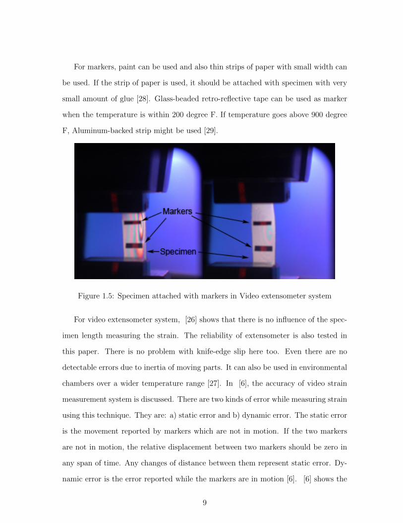
For markers, paint can be used and also thin strips of paper with small width can

be used. If the strip of paper is used, it should be attached with specimen with very

small amount of glue [28]. Glass-beaded retro-reflective tape can be used as marker

when the temperature is within 200 degree F. If temperature goes above 900 degree

F, Aluminum-backed strip might be used [29].

Figure 1.5: Specimen attached with markers in Video extensometer system

For video extensometer system, [26] shows that there is no influence of the spec-

imen length measuring the strain. The reliability of extensometer is also tested in

this paper. There is no problem with knife-edge slip here too. Even there are no

detectable errors due to inertia of moving parts. It can also be used in environmental

chambers over a wider temperature range [27]. In [6], the accuracy of video strain

measurement system is discussed. There are two kinds of error while measuring strain

using this technique. They are: a) static error and b) dynamic error. The static error

is the movement reported by markers which are not in motion. If the two markers

are not in motion, the relative displacement between two markers should be zero in

any span of time. Any changes of distance between them represent static error. Dy-

namic error is the error reported while the markers are in motion [6]. [6] shows the

9

error with respect to the marker size. It is hard to track smaller markers. There is a

optimum width of the marker which can be tracked more accurately, which is beyond

the scope of this thesis. Loading rate is also important for this system. If the loading

rate is high, the error increases [6].

There are also other non-contact techniques to measure the strain of the materials.

The laser speckle extensometer can also be used here. This procedure involves two

dimensional strain measurements in real time. The measuring principle is based on

the analysis of the speckle patterns of the markers when the surface of the specimen is

illuminated by coherent laser light. One or more cameras are used to take the patterns.

Using Fast Fourier Transformation correlation analysis the strain is evaluated [30].

[31] proposed a new extensometer which needs not attachment of line markers or

mechanical tracers on a specimen. Instead of the markers, an expanded beam from a

laser diode was attached on the specimen. [30]

1.8 Polarized light and fringes

Generally, when light waves come directly from a source, the electric field of these

light waves vibrates impartially in all directions at right angles to the wave normal.

When light is polarized, this wave does not vibrate in all directions rather, it vibrates

one or two specific directions. If light is plane polarized, the components of the

vibrations in some plane are transmitted or reflected to the exclusion of the other

components. Our eye is not able to detect such a selection of components. The

intensity is reduced to one half in the most efficient polarizer. However, its rotation

does not cause change in intensity. Again, if a second polarizing device operates

on the polarized light, it will transmit or reflect only the cosine components in its

plane of vibration. This second polarizer is called an analyzer. This is how the

polarization light is created, and with the help of this polarizer light we can see the

10

fringes of the film while it is under load. [32]. There are three kinds of polarization in

Figure 1.6: The polarizer and analyzer effect on natural light and polarized light [

scanned from [5]].

photo elasticity. They are referred to as (a) linearly or plane polarized, (b) circularly

polarized, and (c) elliptically polarized [33]. When all components of the light vector

lie in a single plane, plane polarized or linearly polarized occurs. Circularly polarized

light is obtained when the tip of the light vector moves in a path of circular helix

as light propagates along the direction of from source to destination. Elliptically

polarized light is found when the tip of the light vector describes an elliptical helix.

Certain transparent materials like crystals and stressed plastics have the ability to

resolve an impinging light vector into two orthogonal components. These materials

are used to make the polarizer and analyzer [34]. When a photo-elastic specimen

is placed in a polariscope and subjected to either state of stress and strain, we can

observe isoclinic or isochromatic fringe patterns. If a pohotoelastic model machined

from a sheet of a suitable polymer, it works as an optical element. Initially the model

11

or this specimen is stress-free and exhibits a constant index of refraction at all points.

When load is applied on the model or specimen, a plane state of stress is developed

which changes the optical properties of the model material. The refraction index of

the points of the model or specimen are different from each other. This model become

optically anisotropic and acts as a doubly refraction depend upon the magnitude of

stress at each point in the plate. This is the reason we can see different fringes. It

can be easily found, the mathematical relation between the stress and the change of

refraction indexes. With the help of fringes, we can evaluate the change of refraction

index, and by this we can get the relative stress on the plane. [33]. Even strain analysis

can be performed using moir method [34]. In the article [34], two dimensional strain

measurement is described by using the fringes.

12

CHAPTER 2

METHODOLOGY

2.1 Hardware

For this study, some instruments and tools are used. Those are: INSTRON, Laser

extensometer, cameras, desktop computers, different kinds of lens, polarizer, and an-

alyzer.

2.1.1 INSTRON

The INSTRON is used to apply load in a specimen. This is a universal testing ma-

chine. We can evaluate the mechanical properties of materials and components. For

example, tension, compression, flexure, fatigue, impact, torsion and hardness tests

are the tests we can do with an INSTRON. Though for this study we mainly used the

tension test. The range of the load measured by INSTRON is wide. Using INSTRON

a tension force is applied to film and the preform specimens. There is a load frame

transducer in the INSTRON. The Load frame transducer will measure the load and

generate an electronic AC signal accordingly. Using a data-logger, the digital tension

load of the INSTRON is captured and sent to computer. This is how we can measure

the load given by INSTRON into the computer. [35]

13

2.1.2 Laser Extensometer

A Laser Extensometer is also used to measure displacement optically. Two markers

are placed on the specimen. There is a laser light line which should be place on

those two markers. Using specific settings we can measure the offset displacement of

the two markers. The Laser-extensometer sends the displacement to the data-logger

again. The data-logger then sends this data to a desktop PC. [29]

2.1.3 Computer

A computer was used to run the developed software. Image processing and data

analysis were performed with this same computer. The computer had Core 2 Duo

processor with 2.13 GHz CPU speed. The model of CPUS was Intel(R) Core(TM)2

CPU 6400 series. It had 1 GB physical memory (RAM). The display adapter was

Intel(R) Q965/Q963 Express Chipset Family.

2.1.4 Cameras

For capturing the image of the specimen during the application of load cameras are

used. Two sets of camera with lens are used to take the images. Both of them are

CCD dragonfly cameras. First one is Black and White camera with lens coming with

this camera. This camera has 512x384 resolutions and the frame rate is up to 24

fps. Latter, color camera with several lens are used. This camera’s resolution is

up to 640x480 and it has up to 30 fps. While using color camera different kinds

of lens is used to find the better option. 16mm lens, 32mm lens and 50mm lens is

used to figure out which gives the best result. Using Labview’s Measurement and

Automation Explorer we can have good flexibility to maintain the camera setting.

Exposure, brightness, frame rate, grain, gamma, hue, saturation, sharpness, all of

these can be set to manual (relative), manual (absolute), auto. For different specimen

14

Figure 2.1: 512x384 resolution black and white camera ant its lens.

Figure 2.2: 640x480 resolution color camera and 16mm lens.

we can change these options to get the better results.

2.1.5 Polarizer / Analyzer

To see the fringe change of the film specimen and preform specimen, Polarizer and

Analyzer is used. A polarizer light is generated with a polarizing film. The specimen

is set between the polarizer light and analyzer. From a suitable distance, the camera

is set so that it can capture the fringe change while the specimen is under tension

load. As the light exerted by the light source of that polarizer was not good enough

for this study, we used external light source with high intensity light.

15

Figure 2.3: Polarizer / Analyzer setup.

2.2 Software

Labview is used mainly to interface the hardware. Labview will control the camera

to capture the image. Labview is data-flow programming language. Graphical block

diagrams are used to write the program in this software. The blocks are connected

with wires which propagate the value of variables. When data reach any block,

that block is then executed. Three panels are used in Labview: a block diagram, a

front panel and a connector panel. Controls and indicator is used in the front panel

where operator can input and see the output of the program. Using block diagram,

Figure 2.4: Labview software for this study.

16

the program is written. The algorithms and other special program are written in

this block diagram panel. The main program is called VIs. Many sub-VIS. can be

attached to main VIs files. In our study, we used Labview to get the input picture and

as well as process the image. Implementing the algorithm in block diagram panel,

the image is processed and the outputs are found. The flowchart of the algorithm is

shown in Figure 2.5. Moreover, a user manual of this software was written so that

anybody could learn the software easily.

Figure 2.5: Flowchart of the solftware

17

2.3 Algorithm

The algorithm to track the marker attached on the specimen is implemented in Lab-

view software. Mainly, 3 algorithms are used: pattern learning algorithm, pattern

searching algorithm, measuring displacement algorithm. First, we need to set the

template. To set the template, the program should learn the template first so that

it can recognize it latter. In the pattern learning algorithm of our study, we use

the shape setting to learn the template. After learning, the learned template data

is stored after that this data is used to search. Next algorithm we used is pattern

searching algorithm. In every frame the image is processed so that it can compare

this frame with learned template data. The search technique is used left to right and

then top to bottom. It also uses Bi-linear interpolation while capturing the data.

For measuring the displacement between two markers, timers are uses to start the

Figure 2.6: Block diagram of pattern learning and pattern searching.

measurement technique. The initial displacement is measured in pixels. Latter the

algorithm is developed so that the strain is measured using current displacement and

old saved initial displacement.

18

CHAPTER 3

STRAIN MEASUREMENT TECHNIQUE

In our study, we use different types of algorithms to track the markers. After that,

the comparison is made. In one technique two markers are almost look the same and

only one searching criteria of same markerwas used. However, two different searching

techniques are used in the different approachs. Another approach was tested where

the template was changed dynamically after every specific number of frames.

3.1 Template creation procedure

A template is created by allowing the operator to select the region from the current

image captured by the camera. The operator will select a specific area which will be

later used for searching. There are several ways in our study we used to learn the

template. One way is that operator will select the template image and latter this

image is saved into memory. Another approach is to use the previous saved template

to learn. However, another approach is used to use more than one template to find

the markers. After selecting the template, Labview will learn about the template

and make a data which will then compare with the every frame latter. Using the

shape/color/interpolation technique the template is learned by the Labview software.

In our study, shape is used and Bi-linear interpolation is implemented to scan the

image.

19

Figure 3.1: Template selection and its block diagram

3.2 Strain measurement by searching same template twice.

3.2.1 Technique

In this procedure, almost two identical markers are attached to the specimen with a

small distance separation (usually 15–25 mm). The user will select only one template

to let the software learn about that template. While searching procedure is performed,

the same type of template is searched in every frame twice in the whole image. In this

technique, the software will find two searching areas. Then displacement is measured

by computing the distance between the centers of those two center areas.

Figure 3.2: Strain measurement by searching identical marker twice and its block

diagram.

20

3.2.2 Limitation

The two markers should be the same in shape and in orientation. It is hard to set

both of the markers in same orientation on the specimen. While the specimen started

to deform or under load, one of the template loses its orientation, and that time

this technique could not find the 2 markers separately. Again, there is a change of

orientation and shape accuracy in the program. But if we allow too much orientation

and shape change, sometimes the marker is found in the environment where the

marker is not there but only noise.

3.3 Strain measurement by searching two different templates

3.3.1 Technique

Two different types of markers are attached on the specimen in this procedure. Two

sets of template are learned by the software. For every frame, two search techniques

are performed. One is to find first marker and another is to find second marker.

After processing the frame, two different templates are tracked. The displacement

is measured by calculating the distance of the centers of these two markers found in

each frame. After that, strain is measured by calculation.

Figure 3.3: Strain measurement by searching two different templates.

21

3.3.2 Limitation

If two markers are almost similar, while searching, the program might find same

marker twice. Again, while the specimen is under load or in state of deformed, it even

cannot find any marker at all. Basically, when the specimen is in plastic deformation,

it loses track of the marker as the marker changes or most often, it tracks the same

areas twice.

3.4 Strain measurement by searching two different templates in two

separate regions

3.4.1 Technique

This procedure is like the last procedure. But In this procedure, two templates are

searched in different areas. The region of interest of template 1 differs from the region

of interest of template 2. As the searching areas are different, there is not a possibility

to find the same marker twice. After searching, the displacement is measured in same

technique stated above by calculating the distance between the centers of two different

found areas.

Figure 3.4: Strain measurement by searching two different templates in two separate

regions.

22

3.4.2 Limitation

In this technique the program can track the markers long way, but when the specimen

is under the significant plastic deformation, the markers become so disoriented that

the program could not track them at all.

3.5 Strain measurement by changing the template dynamically

3.5.1 Technique

Like previous stated technique, in this technique the template is learned at the be-

ginning. But unlike other technique, after specific time, the new template is learned.

The last areas found by searching technique are learned to make new templates so

that these new templates are used for latter search. This is how after every specific

time or frames, templates are changing. In this technique, the region of interest is

also set for different markers. In this procedure, the program can track the markers

till the end of the experiment.

Figure 3.5: Strain measurement by changing the template dynamically.

23

3.5.2 Limitation

The process time is slower than others. As the template is changing time to time,

the center of the template changes every time due to orientation of the templates. So

there is possibility to have error in strain measurement.

24

CHAPTER 4

OBSERVING FRINGE UNDER POLARIZED LIGHT

4.1 Instrumental setup

The specimen of film and preform are observed under polarized light. In the polarizer

instrument, generally there is polarizer and analyzer screen. The specimen should be

situated between polarizer and analyzer. However, in our setup only the analyzer

is used. The sample was between the diffuser and the analyzer. At the beginning

the light found from that machine is used to observe the fringe. Latter,the external

high intensity light source is used as shown in the figure. While the INSTRON is

used to perform tensile load on the specimen the polarizer instrument is set such a

way that the camera can have the view of the specimen through the analyzer. The

full experiment is done under this setup. So, the fringe changes and movements are

measured throughout the whole loading time.

Figure 4.1: Instrumental setup for polarized light.

25

4.2 Fringes with low resolution Black & White Camera with its lens

When the black and white camera with resolution 512x384 is used, the fringe is

found as shown in the figure. In this way, the fringes could not be captured well. The

complexion is very ambiguous. That was very hard to track the fringe movement. It

is also hard to decide about any material properties by seeing this images.

Figure 4.2: Fringes captured by low resolution Black & White Camera with its lens.

4.3 Fringes with high resolution color camera with 16mm lens

When the color camera with 16mm lens is used fringes are found just like figure below.

This time fringes are seen well comparing previous scenario. While the specimen is

under the load, the fringe movement can be figure out more accurately than before.

Fringes can be tracked during the experiment. The 16mm lens with good aperture

setting helped to capture the fringes like this.

4.4 Fringes captured using high intensity light sources

The light of the polarizer instrument is replaced by external light. This time lights are

more incandescent. Here the fringes are found like the figures. Here, we can see that

fringes are found in more detail. The movement of the fringe can be observed more

26


accurately than before. Even the degree of the fringes can be measured by capturing

the images.


4.5 Observation of fringe during experiment (sample 1)

During one experiment the fringes are found like the figures. The chronological order

of the fringes can be found if we see the diagram left to right then top to bottom.

This is for a specific sample when external light is not used.

27

Figure 4.5: Observation of fringe during experiment (sample 1).

4.6 Observation of fringe during experiment with external light source

(sample 2) .

During one experiment the fringes are found like the figures. The chronological order

of the fringes can be found if we see the diagram left to right then top to bottom.

This is for a specific sample when external light is used. We can see that the fringes

can be seen more accurately here.

28

Figure 4.6: Observation of fringe during experiment with incandescent external light

source (sample 2).

29

CHAPTER 5

RESULT AND DISCUSSIONS

5.1 Comparison in different technique of strain measurement

Figure 5.1: Comparison for Strain vs Cross-head elongation by searching same tem-

plate twice.

Figure 5.1 shows the comparison for strain vs cross-head elongation curves by

using camera with laser extensometer when same template was searched twice. It is

obvious graph that from the very beginning the two curves are deviating from each

other. More the strain increases the deviation between these two curves becomes

prominent. The deviation of strain using this technique is greater than 15% compare

to that of laser extensometer. The slope of the trend line of the curve for using Laser

30

Extensometer is 0.042 while the slope of the trend line of the curve for using camera

is 0.029. The value of these slope reflected the difference between these two curves.

So, the slopes of the trend line of the curves differ 31% from each other. Most of the

case, it is very hard to make identical markers. So, one marker is learned and using

this data another marker is searched. By allowing the tolerance, two markers have

been tracked. This might be the reason for the deviation of the curve.

On the other hand, Figure 5.2 shows the comparison of strain vs cross head elon-

gation curves by using camera with laser extensometer when two different templates

and two separate regions are selected. In Figure 5.2, both graphs follow almost same

path. The deviation of strain using this technique is less than 5% compare to laser

extensometer. It means, using this technique of searching two different templates

and two separate regions will increase the strain measurement accuracy. Moreover,

the slope of the trend line of the curve for using Laser Extensometer is 0.0285 and

the slope of the trend line of the curve for using camera is 0.0282. So, the slopes of

the trend line of the curves differ 1% from each other. This techniques provide more

consistent result compare to other techniques.

While templates are being changed dynamically, Figure 5.3 is observed. In the

figure, we can see that the deviation of the curved measured by camera and that

of laser extensometer is observed often.Moreover, the slope of the trend line of the

curve for using Laser Extensometer is 0.0177 and the slope of the trend line of the

curve for using camera is 0.0183. So, the slopes of the trend line of the curves differ

3.2% from each other. The strain measured by camera is not consistent compare

to other techniques. When the templates are searched and changed after specific

times, the centers of the templates with respect to the shape of templates deviate

every time. This is why Figure 5.3 shows inconsistent measurement of strain by

31

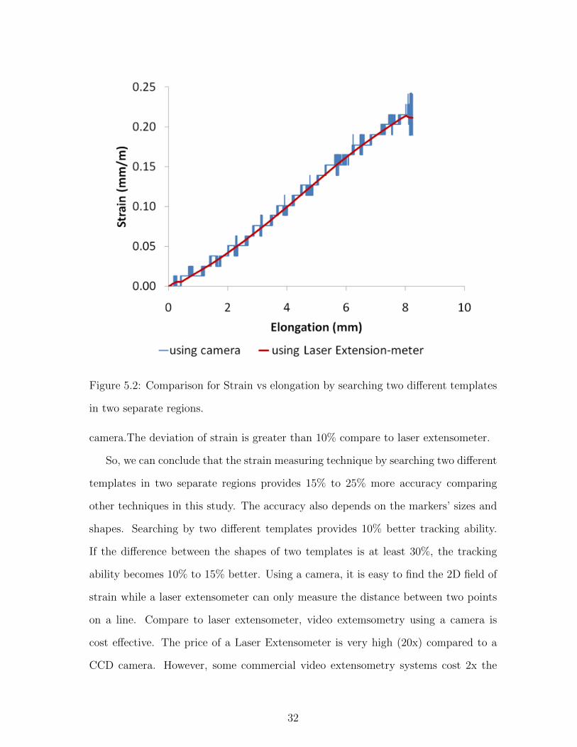
Figure 5.2: Comparison for Strain vs elongation by searching two different templates

in two separate regions.

camera.The deviation of strain is greater than 10% compare to laser extensometer.

So, we can conclude that the strain measuring technique by searching two different

templates in two separate regions provides 15% to 25% more accuracy comparing

other techniques in this study. The accuracy also depends on the markers’ sizes and

shapes. Searching by two different templates provides 10% better tracking ability.

If the difference between the shapes of two templates is at least 30%, the tracking

ability becomes 10% to 15% better. Using a camera, it is easy to find the 2D field of

strain while a laser extensometer can only measure the distance between two points

on a line. Compare to laser extensometer, video extemsometry using a camera is

cost effective. The price of a Laser Extensometer is very high (20x) compared to a

CCD camera. However, some commercial video extensometry systems cost 2x the

32

Figure 5.3: Comparison for Strain vs elongation by searching two different dynami-

cally changed templates in two separate regions.

laser system. Figure 5.4 shows the comparison of strain measured by the camera

with INSTRON when two different templates are searched in two separate regions.

The percentages of error are also reflected in Figure 5.5. It can be seen that when

the initial length increases, the percentage of error decreases. We can also observe

that the percentages of error for the 640x480 pixel cameras are generally less that

5%. If the resolution of the camera increases, the error might be even less, however

the difference between methods tested here would still be relevant.

5.2 Observation of fringes under polarized lights

It is observed that the fringes change due to increase of stress. The fringe becomes

thinner while more stress is applied which means that the stress upon the whole

area is also increasing. By using fringes , the stress distribution through the 2D

33

Figure 5.4: Comparison of strain measured by the cam and INSTRON by varying

initial length.

space can be measured with accurate calculation. This is why the observation of

fringes contribute an important role in the experimental mechanics. When the stress

increases the refractive index of PET changes which will change the fringes.

In Figure 5.7(a), Figure 5.7(b), Figure 5.8(a) and Figure 5.8(b), Stress vs Strain

Curves are shown. The points when the fringes disappear for every curves are also

shown by star marks. All these curves are shown in Figure 5.6.

Generally, there is some permanent deformation in the PET like crazing that

caused scattering so that visible light does not penetrate well. Then the optical

polarization is broken up and the fringes disappear. It is interesting that the fringes

disappear at similar stresses on each of the graphs and that is near at yield point.

It is also clear that after plastic deformation some non-linearity is observed in the

change of the fringe spacing. It is also observed that fringes will change more during

the linear part of the curve and less in the plastic part of the curve. In Figure 5.6,

34

Figure 5.5: Error percentage of strain measured by the cam and INSTRON by varying

initial length.

the slopes of the curves are slightly different from each other. This might be due to

the change of the pressure difference of the gripper which hold the specimen during

the experiments.

35

Figure 5.6: Stress vs Strain Curves.

(a) Stress-Strain Curve (sample 1). (b) Stress-Strain Curve (sample 2).

Figure 5.7: Stress-Strain Curve showing the point when fringes disappear.

36

(a) Stress-Strain Curve (sample 3). (b) Stress-Strain Curve (sample 4).

Figure 5.8: Stress-Strain Curve showing the point when fringes disappear.

37

CHAPTER 6

CONCLUSIONS

• LabVIEW code developed here is successful at performing video exntesometry.

• The technique where strain was measured using two different templates in two

separate regions had 15% to 25% more accuracy comparing other techniques in

this study. Here, changing the template dynamically did not give good results.

• If two different templates were used to measure the distance between them, the

accuracy of tracking the marker became 10% better.

• If the difference between the shapes of two templates is at least 30%, the tracking

ability becomes 10% to 15% better when searching two different templates are

used.

• The accuracy of the slope of trend line of proposed technique was 99% using a

camera with 640x480 resolutions compared to Laser Extensometer.

• The error of measuring strains was generally less than 5% when a camera with

640x480 resolutions was used. Higher resolution cameras have the ability to

measure strain more accurately, but the difference between methods tested here

would still be relevant.

• Compared to the Laser Extensometer, video extensometry using a camera is

cost effective. The price of a Laser Extensometer is very high (20x) compared

to a CCD camera. However some commercial video extensometry systems cost

2x the laser system.

38

• A laser Extensometer can only measure the distance between two points on a

line. Using a camera, it is easy to find the 2D field of the strain.

• By using a camera, the strain can be measured on-line. However, by capturing

images with a camera, strain can be measured off-line also. Cracking, fringes,

or other behavior can also be studied.

• A camera provides a good opportunity to observe the fringes when the PET is

under polarized light.

• It is observed that before the yield point the fringes disappear. The fringes

disappear due to permanent deformation in the PET. So, by observing the

fringes, we may find when the permanent deformation occurs.

39

CHAPTER 7

FUTURE WORK

• The developed software can be extended to sub-pixel level.

• Image Calibration can be included in the developed software.

• Using zoom lens with a higher resolution camera, the accuracy of the proposed

technique can be verified more accurately.

• The developed software can be extended to make it suitable for determining the

Poissons Ratio.

• The Software can be updated such a way that can measure the fringe width.

• Validation of relationship between the fringes and deformation is another good

scope of this study.

40

BIBLIOGRAPHY

[1] H. W. S. Michael A. Sutton, Jean-Jos Orteu, Image Correlation for Shape and

Deformation Measurements: Basic Concepts, Theory and Applications, pp. 17–

21. Springer, 1st ed., 2009.







[4] F. M. P. C. Mark D. Bethea, James A. Lock, “Three-dimensional camera cali-

bration technique for stereo imaging velocimetry experiments,” OPTICAL EN-

GINEERING, vol. 36, no. 12, pp. 3445–3454, 1997.

[5] F. W. Sears, Principles of physics series: Optics, pp. 167–202. Addison Wesley

Press, Inc, 3rd ed., 1949.

[6] L. J. B. E. G. W.P. Smutz, M. Drexler and K. An, “Accuracy of a video strain

measurement system.,” J. Biomechanics, vol. 29, no. 6, pp. 813–817, 1996.

[7] E. Hecht and A. Zajac., Optics. Addison-Wesley, Reading, MA,, 1st edition ed.,

1974.

41

[8] L. C. Weiwei Feng, “Relative orientation accuracy analysis of the polarizers in a

polarization ccd camera,” Optik - International Journal for Light and Electron

Optics, vol. 121, pp. 1401–1404, 2010.




[10] H. Lu and P. D. Cary, “Deformation measurements by digital image correla-

tion: Implementation of a second-order displacement gradient,” Experimental

Mechanics, vol. 40, no. 4, pp. 393–400, 2000.

[11] S. Periasamy, “Digital image correlation for deformation measurements near a

crack,” Thesis, 2002.

[12] W. Peters and W. Ranson, “Digital imaging techniques in experimental stress

analysis.,” Opt. Eng., vol. 21, pp. 427–432, 1982.

[13] W. W.-P. W. R. W. Sutton, M.A. and S. McNeil, “Determination of displace-

ments using an improved digital image correlation method,” Image Vision Com-

puting, vol. 1, no. 3, pp. 133–139, 1983.

[14] C. M.-P. W. C. Y. Sutton, M.A. and S. McNeil, “Application of an optimized

digital image correlation method to planar deformation analysis,” Image Vision

Computing, vol. 4, no. 3, pp. 143–150, 1986.

[15] M. S. S. M. Bruck, H.A. and W. Peters, “Digital image correlation using

newton-raphson method of partial differential correction,” EXPERIMENTAL

MECHANICS, vol. 29, pp. 26–267, 1989.

42

[16] C. Y. s. M. Luo, P.F. and W. Peters, “Accurate measurement of three-

dimensional deformations in deformable and rigid bodies using computer vision,”

EXPERIMENTAL MECHANICS, vol. 33, pp. 123–132, 1993.

[17] G. Vendroux and W. Knauss, “Submicron deformation field measurements: Part

1, developing a digital scanning tunneling microscope,” EXPERIMENTAL ME-

CHANICS, vol. 38, pp. 18–23, 1998.

[18] G. Vendroux and W. Knauss, “Submicron deformation field measurements:

Part2: Improved digital image correlation,” EXPERIMENTAL MECHANICS,

vol. 38, pp. 86–91, 1998.

[19] G. Vendroux and W. Knauss, “Submicron deformation field measurements:

Part 3. demonstration of deformation determinations,” EXPERIMENTAL ME-

CHANICS, vol. 38, pp. 154–60, 1998.

[20] G. Vendroux, “Correlation: A digital image correlation program for displacement

and displacement gradient measurements,” GALCIT Report No. SM90-19, 1990.

[21] J. L. J.S. Lyons and M. Sutton, “High-temperature deformation measurement us-

ing digital-image correlation,” EXPERIMENTAL MECHANICS, vol. 36, no. 1,

pp. 64–70, 1996.

[22] K. K. Satoru Yoneyama, Akikazu Kitagawa and H. Kikuta, “In-plane displace-

ment measurement using digital image correlation with lens distortion correc-

tion,” JSME International Journal, vol. 49, no. 3, pp. 458–467, 2006.

[23] G. V. H. Lu and W. G. Knauss, “Surface deformation measurements of a cylin-

drical specimen by digital image correlation,” EXPERIMENTAL MECHANICS,

vol. 37, no. 4, pp. 433–439, 1997.

43

[24] H. X. Bing Pan, Kemao Qian and A. Asundi, “Two-dimensional digital image

correlation for in-plane displacement and strain measurement: a review,” Mea-

surement Science & Technology, vol. 20, no. 6, 2009.

[25] V. T. H. S. J. O. M.A. Sutton, J.H. Yan, “The effect of out-of-plane motion on

2d and 3d digital image correlation measurements,” OPTICS AND LASERS IN

ENGINEERING, vol. 46, no. 11, pp. 746–757, 2008.

[26] K. K. D. Coimbra, R. Greenwood, “Tensile testing of ceramic fibres by video

extensometry,” Journal of Materials Science, vol. 35, no. 13, pp. 3341–3345,

2000.

[27] V. G. Ph Franois and R. Sgula, “Local-scale analysis of the longitudinal strains in

strongly necking materials by means of video-controlled extensometry,” JOUR-

NAL OF PHYSICS-CONDENSED MATTER, vol. 6, no. 42, pp. 8959–8968,

1994.

[28] A. B. M. Wolverton and G. Kannarpady, “Efficient, flexible, noncontact de-

formation measurements using video multi-extensometry,” EXPERIMENTAL

TECHNIQUES, vol. 33, no. 2, pp. 24–33, 2009.

[29] E. I. Research, “Laser extensometers,” Dec 2010. http://www.e-i-r.com/.

[30] P. R. Laraba-Abbes F, lenny P, “Determination of rivlin parameters for car-

bon black filled nr using laser speckle extensometer,” KAUTSCHUK GUMMI

KUNSTSTOFFE, vol. 52, pp. 209–214, 1999.

[31] I. T. Y. M. Yamaguchi I, Kobayashi K, “Noncontacting extensometer using dig-

ital speckle correlation,” MATERIALS EVALUATION, vol. 64, pp. 724–730,

2006.

44

[32] J. Valasek, Introduction to theoretical and experimental optics, pp. 196–241. John

Wiley and Sons Inc, 1st ed., 1949.

[33] J. W. D. Felix Zandman, Salomon Render, Photoelastic Coatings, pp. 1–30. Sci-

ence Press, 1st ed., 1977.

[34] P. S. Theocaris, Moir Fringes in Strain Analysis, pp. 147–177. Pergamon press,

1st ed., 1969.

[35] INSTRON, “Instron, the difference is measurable,” Dec 2010.

http://www.instron.us/wa/home/.

[36] J.-H. P. Jong-Eun Ha and D.-J. Kang, “New strain measurement method at axial

tensile test of thin films through direct imaging,” JOURNAL OF PHYSICS D-

APPLIED PHYSICS, vol. 41, no. 17, pp. 3341–3345, 2008.

[37] U. T. Systems, “Optical extensometer - features, performance and applications

of laser extensometer.”,” 2010.

[38] M.-S. S. S.-J. L. S.-C. Y. K.-S. L. J.-E. H. S.-H. c. Jun-Hyup Park, Dong-

Joong Kang, “Easy calibration method of vision system for in-situ measurement

of strain of thin films,” TRANSACTIONS OF NONFERROUS METALS SO-

CIETY OF CHINA, vol. 19, pp. S243–S249, 2009.

45

VITA

Mazarul Islam

Candidate for the Degree of

Master of Science

Thesis: DEVELOPING VIDEO MEASUREMENT OF STRAIN FOR POLYMERSUSING LABVIEW

Major Field: Mechanical & Aerospace Engineering

Biographical:

Personal Data: Born in Dhaka, Bangladesh on December 3, 1982.

Education:Received the B.S. degree from Bangladesh University of Engineering &Technology (BUET),Dhaka, Bangladesh, 2008, in Mechanical EngineeringCompleted the requirements for the degree of Master of Science with amajor in Mechanical & Aerospace Engineering Oklahoma State Universityin December, 2010.

Experience:Worked as a teachers assistant for an undergraduate course (2009 & 2010).Worked as a research assistant under supervision of Dr. Jay Hanan for 2years.

Name: Mazharul Islam Date of Degree: May, 2011

Institution: Oklahoma State University Location: Stillwater, Oklahoma

Title of Study: DEVELOPING VIDEO MEASUREMENT OF STRAIN FORPOLYMERS USING LABVIEW

Pages in Study: 45 Candidate for the Degree of Master of Science

Major Field: Mechanical & Aerospace Engineering

The purpose of this study was to develop a computer assisted video extensometer tomeasure strain, primarily for transparent polymers such as PET. Two markers, whichwere attached to the specimen, were tracked by the video system. Different techniqueswere proposed to track these markers implemented in NI LabVIEW software. Theaccuracy of video extensometry depends on the template creation procedure, shapesof the markers, algorithm and camera resolution. Comparison of the different tech-niques was discussed in this study. The technique with two different templates intwo separate regions provided 15% to 25% more accuracy compared to other tech-niques discussed in this study. The accuracy of the proposed video extensometerwas also shown. The accuracy of the proposed technique was 99% using a camerawith 640x480 resolution. Moreover, comparison with a Laser Extensometer and theproposed video extensometer were also shown. Fringes were also captured when thePET was in tensile stress and under polarized light. The pattern-changes of thesefringes were recorded by NI LabVIEW software. The disappearance of fringes beforethe yield point in tension indicated permanent plastic deformation in PET.

ADVISOR’S APPROVAL:

developing video measurement of strain for

Documents