developing financial distress prediction models 2006/07as-127-developin… · developing financial...

Developing Financial Distress Prediction Models: Yu-Chiang Hu and Jake Ansell (2006) 1

Developing Financial Distress Prediction Models

A Study of US, Europe and Japan Retail Performance

Yu-Chiang Hua,1

and Jake Ansella

aManagement School and Economics, University of Edinburgh, William Robertson Building, 50 George Square, Edinburgh, EH8 9JY, UK

Abstract

This paper constructs retail financial distress prediction models based on five key variables previously shown

to have good classification properties (Hu and Ansell, 2005). Five credit scoring techniques—Naïve Bayes,

Logistic Regression, Recursive Partitioning, Artificial Neural Network, and Sequential Minimal Optimization

(SMO) were considered. A sample of 491 healthy firms and 68 distressed retail firms were studied over a five-

year time period from 2000 to 2004.

An international comparison analysis of three retail market models –USA, Europe and Japan– shows that the

average accuracy rates are above 86.5% and the average AUROC values are above 0.79. Almost all market

models display the best discriminating ability one year prior to financial distress. The US market model

performs relatively better than European and Japanese models five years before financial distress.

A composite model is constructed by combining data from US, European and Japanese markets. All five

credit-scoring techniques have the best classification ability in the year prior to the financial distress, with

accuracy rates of above 88% and AUROC values of above 0.84. Furthermore, these techniques still remain

sound five years before financial distress, as the accuracy rate is above 85% and AUROC value is above 0.72.

However, it is difficult to conclude which modelling technique has the absolute best classification ability, since

the composite model’s performance varies according to different time scales.

Regarding the applicability of the composite model, a comparison is made using Moody’s credit ratings.

Results indicate that SMO is the better performing model amongst the three models, closely followed by the

neural network model. Logistic regression model shows lowest performance in terms of similarity with

Moody’s.

Keywords: Credit Risk, Financial Distress Prediction; Multivariate statistics; Artificial intelligence

1 Corresponding author

Email address: [email protected] (Yu-Chiang Hu), [email protected] (Jake Ansell)

* Acknowledgement: This research is funded by the College of Humanities and Social Science, Management School and

Economics at University of Edinburgh as well as the Overseas Research Students Awards Scheme (ORSAS).


1. Introduction

How can financial distress be predicted? This question is of interest not only to managers

but also to external stakeholders of a company. These players are continuously seeking the

optimal solution for performance forecasting, as a way to rationalize the decision-making

process. Thus, the primary objective of this paper is to establish financial distress prediction

models based on credit-scoring techniques.

A single industry is chosen to avoid generalizations across industries. The retail industry is

selected, as assessing and evaluating retail risk is one of the key issues in retail research

(Dawson, 2000). Variable selection is derived from findings in Hu and Ansell (2005). Based

on a USA retail dataset of 195 healthy firms and 51 distressed firms for years 1994 to 2002,

Hu and Ansell (2005) showed that five critical performance variables: Debt Ratio, Total Debt

/ (Total Debt + Market Capitalization), Total Assets, Operating Cash Flow and Government

Debt / GDP have sound classification ability (accuracy rate of above 90% and AUROC value

of above 0.935) one year before financial distress. Moreover, even if the time period is five

years prior to financial distress, the classification accuracy rate using these variables is above

80% and the AUROC value is above 0.80.

This research employs five credit-scoring techniques: Naïve Bayes, Logistic Regression,

Recursive Partitioning, Artificial Neural Network, and Sequential Minimal Optimization

(SMO) for modelling purposes. Three target markets, USA, Europe and Japan, are selected

for an international comparison analysis. Comparative results show that regardless of the

target countries, the average accuracy rates are above 86.5% and the average AUROC values

are above 0.79. Moreover, exploring the time dimension, all three market models perform

best in the year prior to financial distress with slight difference across markets. However, the

longer the period before financial distress, the greater the difference across markets becomes,

especially in terms of the AUROC values. For example, five years prior to financial distress,

the US has significantly better AUROC value than Japan or Europe.

The research develops a composite model based on a sample of 491 healthy and 68

distressed retail firms over the time period from 2000 to 2004 by combining data from the

USA, Europe and Japan. Results show that all five credit-scoring techniques in the year prior

to the financial distress display the best performance with accuracy rates of above 88% and

AUROC values of above 0.84. Furthermore, these techniques still remain sound five years

before financial distress, as the accuracy rate is above 85% and AUROC value is above 0.72.


However, it is difficult to conclude which modelling methodology has the absolute best

classification ability, since the model’s performance varies in terms of different time scales.

Finally, in order to examine potential overfitting problems in the composite model, a

comparison of the composite model with Moody’s credit rating is carried out. The results

indicate that SMO is the better performing model amongst the three models, closely followed

by neural network model. Logistic regression model shows lowest performance in terms of

similarity with Moody’s.

Financial distress prediction modelling techniques will be discussed in section 2. Section 3

will illustrate the variable selection and data collection. Section 4 describes the

methodologies employed to evaluate modelling utility and compare results with Moody’s

rating. The results will be analyzed in section 5. Finally, a discussion of the results will be

presented in section 6.

2. The Development of Default Prediction Modelling Techniques

Financial distress prediction became a critical accounting and finance research area since

1960s. Based on the cash flow framework, Beaver carried out three different univariate

analyses—profile analysis (comparison of mean values), dichotomous classification test and

likelihood ratio analysis— in order to examine the predictive characterises and utility of each

variable. Regarding the likelihood ratio analysis, Beaver (1966) conducted an analysis of

likelihood ratios based on the Bayesian approach. He argued that the default prediction

problem could be regarded as a problem of evaluating the probability of financial distress

conditional upon the value of a specific financial ratio. He further pointed out that financial

ratios can provide useful information for predicting default, since the likelihood ratios still

present high values even five years prior to financial distress. Let D represents the distressed

sample and X is the vector of independent variables and assume x is a particular vector of an

independent variable. The conditional probability of a financial distress company in terms of

a specific financial ratio x can be expressed as:

)(

)|()()|(

xXP

DxXPDPxXDP

=

=== (1)

Univariate analysis is limited in the evaluation of a firm’s performance, since it is difficult

to use only one single measure to describe the performance in a multidimensional firm.


However, prior to construct a multivariate model, it is still useful to carry out a univariate

analysis for the purpose of variable selection, as not every variable has good discriminating

utility (Hosmer and Lemeshow, 2000).

Altman (1968) was the first researcher to apply the Multiple Discriminant Analysis (MDA)

approach to the financial distress prediction domain. He developed a Z-score bankruptcy

prediction model and determined a cutpoint of Z-score (2.675) to classify healthy and

distressed firms. The results showed that the Z-score model had sound prediction

performance one year and two years before financial distress, but did not indicate good

prediction utility three to five years before financial distress. A number of authors followed

his work, and applied the Z-score model into different markets, different time periods and

different industries, such as, Taffler (1982, 1984), Pantalone and Platt (1987), Betts and

Belhoul (1987) and Piesse and Wood (1992).

However, MDA assumes that the covariance matrices of two populations are identical and

both populations need to be described by multivariate normal distribution. Clearly, these

assumptions do not always reflect the real world. Deakin (1976) argued that even if after

performing the normality transforming process, financial ratio data do not follow normal

distribution. Moreover, Hamer (1983) evaluated the sensitivity of financial distress prediction

models in terms of four different variable sets from previous research (Altman, 1968; Deakin,

1972; Blum, 1974; Ohlson, 1980) and she pointed out that the covariance matrices in each

variable set were statistically different.

Ohlson (1980) was the first to apply the Logistic Regression model to financial distress

prediction research. After Ohlson’s (1980) work, the conditional probability model became a

popular modelling technique in the bankruptcy prediction domain (also see Zavgren, 1983;

Mensah, 1983; Casey and Bartczak, 1985) The logistic regression model can be linearized by

logit transformation on odd ratio function and can be expressed as follow:

nn xxxx

xxg ββββ

π

π++++=�

�

��

�

−= ...

)(1

)(ln)( 22110

(2)

Tx×= β

Where �(x) is the logistic function,

T

T

T x

x

xe

e

ex

×

×

×− +=

+=

β

β

βπ

11

1)(

)(

(3)


Although logistic regression does not suffer from the limitations of MDA, Tabachnick and

Fidell (2000) pointed out that if the assumptions regarding the identical covariance matrices

and multivariate normal distribution are met, MDA is likely to be more efficient than logistic

regression. Moreover, like all the regression functions, the problem of multicollinearity still

exists in logistic regression.

Recursive Partitioning (RP) was introduced in the bankruptcy prediction research in the

mid-1980s (Marais et al., 1984; Frydman et al., 1985). RP is a non-parametric technique and

does not suffer the limitations from traditional statistical models. Based on the lowest

expected misclassification cost, RP first selects an independent variable as the best

discriminator and decides a cutpoint. The next step is to classify both healthy and distressed

firm into two sub-nodes in terms of the cutpoint. The third step is to select another (or the

same) discriminator and further partition the healthy and distressed firms into another two

sub-nodes. The same process can be continued, if further splitting is necessary. It is obvious

that the overfitting may be a potential problem of RP, since the continuous partitioning

process is likely to encourage one misclassified case in the terminal node. Therefore, Thomas

et al. (2002) pointed out that if the sample size in a node is too small, then further partition is

not appropriate. Moreover, if the classification difference between the old node and new

nodes is not significant, the partitioning process is not necessary to continue.

From the late 1980s, the Machine Learning techniques in the Artificial Intelligence (AI)

area, such as Artificial Neural Networks (ANN), were applied to financial distress prediction

studies (Coates and Fant, 1993; Zhang et al., 1999). The most popular ANN algorithm in the

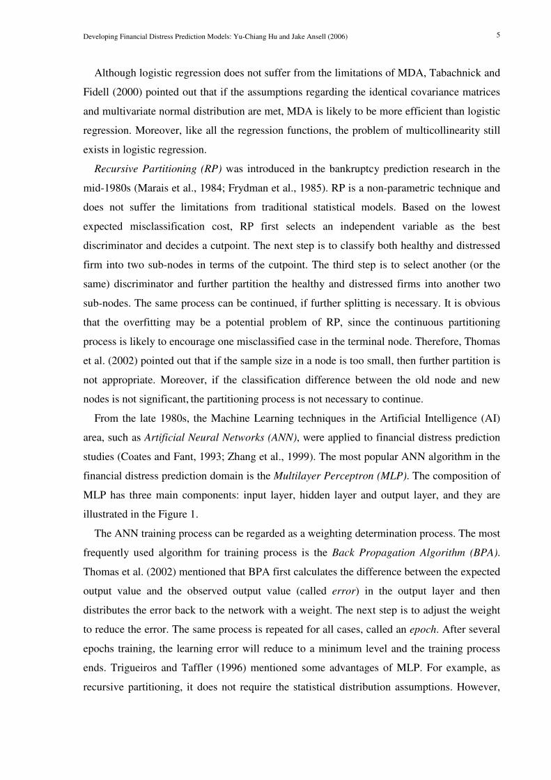
financial distress prediction domain is the Multilayer Perceptron (MLP). The composition of

MLP has three main components: input layer, hidden layer and output layer, and they are

illustrated in the Figure 1.

The ANN training process can be regarded as a weighting determination process. The most

frequently used algorithm for training process is the Back Propagation Algorithm (BPA).

Thomas et al. (2002) mentioned that BPA first calculates the difference between the expected

output value and the observed output value (called error) in the output layer and then

distributes the error back to the network with a weight. The next step is to adjust the weight

to reduce the error. The same process is repeated for all cases, called an epoch. After several

epochs training, the learning error will reduce to a minimum level and the training process

ends. Trigueiros and Taffler (1996) mentioned some advantages of MLP. For example, as

recursive partitioning, it does not require the statistical distribution assumptions. However,


MLP still has some limitations, such as no adequate significance tests and requirement of

computer power (Tam and Kiang, 1992).

Input layer Hidden layer Output layer

Figure 1 Three Layers Multilayer Perceptron

The input layer is responsible for receiving information from the outside environment and

transferring it to the hidden layer. In the hidden layer, a neuron will assign a series of weights

to the inputs, cope with the information via a training process, and then forward the results with

weights to the output layer.

In the late 1990s, Support Vector Machine (SVM) was introduced to cope with the

classification problem. Fan and Palaniswami (2000) applied SVM to select the financial

distress predictors. They pointed out that SVM created an optimal separating hyperplane in

the hidden feature space in terms of the principle of structure risk minimization and used the

quadratic programming to obtain an optimal solution. However, Platt (1999) argued that a

large number of quadratic programming in SVM training is time consuming. As a result, he

introduced a new algorithm, Sequential Minimal Optimization (SMO), to improve the SVM

training time, since SMO only uses two Lagrange multipliers at each training step. Plat (1999)

also pointed out that SMO has better performance than other SVM training methods in terms

of many aspects, such as better scaling with training sample size. From the early 2000s, some

other credit scoring modelling techniques were also employed in the bankruptcy prediction

research area and have shown good performance, including the Rough Sets approach (McKee,

2003) and the Multidimensional Scaling approach (Mar-Molinero and Serrano-Cinca, 2001).


3. Variable Selection and Data Collection

3.1 Variable Selection

Hu and Ansell (2005) developed a theoretical framework for retail performance measure

selection based on Hunt’s (2000) Resource-Advantage (R-A) Theory of Competition and 170

potential retail performance measures, which cover both internal and external measures, were

obtained in terms of previous literature survey and interviews with outside stakeholders. In

this framework, Hu and Ansell (2005) considered several important aspects relative to

variable selection in the previous bankruptcy prediction studies. For example, some studies

pointed out that the macro-economical factors have great impacts on a default prediction

model (Rose et al., 1982; Mensah, 1984). Hu and Ansell (2005) considered the external

variables not only based on the economical environment, but also took into account the

political environment, social-culture environment and technological environment.

Moreover, they also considered the qualitative performance measures in terms of the

practical point of view, since many renowned credit-rating companies including Moody’s,

S&P, and Fitch consider both quantitative and qualitative factors when carrying out credit

evaluation but attribute more importance to qualitative rather than quantitative factors in the

process (Moody’s, 1998 and 2002; Fitch, 2000 and 2001; S&P, 2002 and 2003). In addition,

the industrial variables, such as store number, were also contemplated in their framework,

since some authors argued that the industry-relative measures could improve the accuracy of

the classification model (Platt and Platt, 1990).

Although Hu and Ansell (2005) took into account many potential performance measures, it

is obvious that too many variables in a prediction model tend to overfit the model utility, and

hence provides a subjective conclusion. Drawing on this insight, they selected key

performance measures by using the logistic forward stepwise analysis. In addition, prior to

select the final variables, some key issues include: time-scale consideration, outlier

elimination and univariate analysis, were carried out in order to ensure the quality of key

variables. The results provided sufficient evidence that that these five variables have sound

classification ability (accuracy rate is above 90% and AUROC value is above 0.935) one

year prior to financial distress. Furthermore, even if the time period is five years prior to

financial distress, the classification accuracy rate using these variables is above 80% and the

AUROC value is above 0.80. These five key variables are illustrated as follows:


(1) Leverage Measures: Debt Ratio and Total Debt / (Total Debt + Market Capitalization)

Debt Ratio and Total Debt / (Total Debt + Market Capitalization) are used to evaluate a

company’s leverage situation, especially to measure a company’s ability to face its long-term

obligations. Therefore, these two measures are related to a company’s credit assessment

directly. One of the differences between these two measures is equity evaluation. For debt

ratio (total debts / total assets), the value of equity is evaluated by accounting value, whilst

the equity value is evaluated by market value for another leverage measure.

Another difference between these two measures is the maximum value. For the ratio of

total debt / (total debt + market capitalization), the maximum value is one, since the

minimum value of the market capitalization is zero. However, for the debt ratio, the

maximum value is possible to greater than one, since the value of total debt is possible to

greater than the value of total assets. It implies that even if a company sell all its assets, this

company still cannot cover their future obligations. In fact, if a company’s debt ratio is

greater than one, this company is under the stock-based insolvency situation (Altman 1983,

Ross, et al. 1999). In other words, this company is currently facing financial distress.

However, a higher leverage may not mean a higher bad debt risk, since it depends on the

composition of the leverage. Fitch (2000) argued that distinguishing the financial leverage

and operating leverage is very important in the retail industry, since the operating leverage,

such as the loan for store equipments purchasing, is caused by the customer’s demand, and

hence not so risky. Drawing on this insight, leverage analysis should focus on financial

leverage rather than operating leverage.

(2) Scale Measure: Total Assets

Scale measures are more important in the retail industry than in other industries, as one of

the important characteristics in the retail industry is low-margin. Large firms usually have

certain advantages, which small firms do not have. For example, large firms have better risk

endurance when the economical situation changes. Moreover, large firms also have better

financial flexibility, since they can more easily ask for a loan from a financial institution than

small firms (S&P, 2003). As a result, size is a significant variable for evaluating a retailer’s

credit risk.


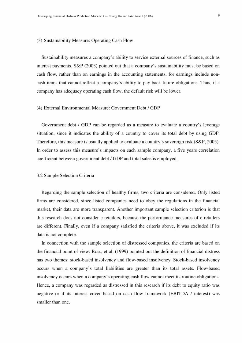
(3) Sustainability Measure: Operating Cash Flow

Sustainability measures a company’s ability to service external sources of finance, such as

interest payments. S&P (2003) pointed out that a company’s sustainability must be based on

cash flow, rather than on earnings in the accounting statements, for earnings include non-

cash items that cannot reflect a company’s ability to pay back future obligations. Thus, if a

company has adequacy operating cash flow, the default risk will be lower.

(4) External Environmental Measure: Government Debt / GDP

Government debt / GDP can be regarded as a measure to evaluate a country’s leverage

situation, since it indicates the ability of a country to cover its total debt by using GDP.

Therefore, this measure is usually applied to evaluate a country’s sovereign risk (S&P, 2005).

In order to assess this measure’s impacts on each sample company, a five years correlation

coefficient between government debt / GDP and total sales is employed.

3.2 Sample Selection Criteria

Regarding the sample selection of healthy firms, two criteria are considered. Only listed

firms are considered, since listed companies need to obey the regulations in the financial

market, their data are more transparent. Another important sample selection criterion is that

this research does not consider e-retailers, because the performance measures of e-retailers

are different. Finally, even if a company satisfied the criteria above, it was excluded if its

data is not complete.

In connection with the sample selection of distressed companies, the criteria are based on

the financial point of view. Ross, et al. (1999) pointed out the definition of financial distress

has two themes: stock-based insolvency and flow-based insolvency. Stock-based insolvency

occurs when a company’s total liabilities are greater than its total assets. Flow-based

insolvency occurs when a company’s operating cash flow cannot meet its routine obligations.

Hence, a company was regarded as distressed in this research if its debt to equity ratio was

negative or if its interest cover based on cash flow framework (EBITDA / interest) was

smaller than one.


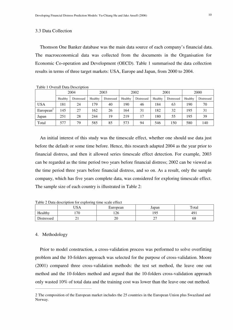
3.3 Data Collection

Thomson One Banker database was the main data source of each company’s financial data.

The macroeconomical data was collected from the documents in the Organisation for

Economic Co-operation and Development (OECD). Table 1 summarised the data collection

results in terms of three target markets: USA, Europe and Japan, from 2000 to 2004.

Table 1 Overall Data Description

2004 2003 2002 2001 2000

Healthy Distressed Healthy Distressed Healthy Distressed Healthy Distressed Healthy Distressed

USA 181 24 179 40 190 46 184 63 190 70

European2 145 27 162 26 164 31 182 32 195 31

Japan 251 28 244 19 219 17 180 55 195 39

Total 577 79 585 85 573 94 546 150 580 140

An initial interest of this study was the timescale effect, whether one should use data just

before the default or some time before. Hence, this research adapted 2004 as the year prior to

financial distress, and then it allowed series timescale effect detection. For example, 2003

can be regarded as the time period two years before financial distress; 2002 can be viewed as

the time period three years before financial distress, and so on. As a result, only the sample

company, which has five years complete data, was considered for exploring timescale effect.

The sample size of each country is illustrated in Table 2:

Table 2 Data description for exploring time scale effect

USA European Japan Total

Healthy 170 126 195 491

Distressed 21 20 27 68

4. Methodology

Prior to model construction, a cross-validation process was performed to solve overfitting

problem and the 10-folders approach was selected for the purpose of cross-validation. Moore

(2001) compared three cross-validation methods: the test set method, the leave one out

method and the 10-folders method and argued that the 10-folders cross-validation approach

only wasted 10% of total data and the training cost was lower than the leave one out method.

2 The composition of the European market includes the 25 countries in the European Union plus Swaziland and

Norway.


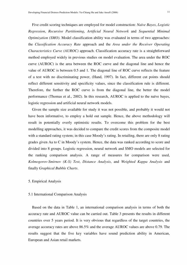
Five credit scoring techniques are employed for model construction: Naïve Bayes, Logistic

Regression, Recursive Partitioning, Artificial Neural Network and Sequential Minimal

Optimization (SMO). Model classification ability was evaluated in terms of two approaches:

the Classification Accuracy Rate approach and the Area under the Receiver Operating

Characteristics Curve (AUROC) approach. Classification accuracy rate is a straightforward

method employed widely in previous studies on model evaluation. The area under the ROC

curve (AUROC) is the area between the ROC curve and the diagonal line and hence the

value of AUROC is between 0.5 and 1. The diagonal line of ROC curve reflects the feature

of a test with no discriminating power, (Hand, 1997). In fact, different cut points should

reflect different sensitivity and specificity values, since the classification rule is different.

Therefore, the further the ROC curve is from the diagonal line, the better the model

performance (Thomas et al., 2002). In this research, AUROC is applied to the naïve bayes,

logistic regression and artificial neural network models.

Given the sample size available for study it was not possible, and probably it would not

have been informative, to employ a hold out sample. Hence, the above methodology will

result in potentially overly optimistic results. To overcome this problem for the best

modelling approaches, it was decided to compare the credit scores from the composite model

with a standard rating system; in this case Moody’s rating. In retailing, there are only 8 rating

grades given Aa to C in Moody’s system. Hence, the data was ranked according to score and

divided into 8 groups. Logistic regression, neural network and SMO models are selected for

the ranking comparison analysis. A range of measures for comparison were used,

Kolmogorov-Smirnov (K-S) Test, Distance Analysis, and Weighted Kappa Analysis and

finally Graphical Bubble Charts.

5. Empirical Analysis

5.1 International Comparison Analysis

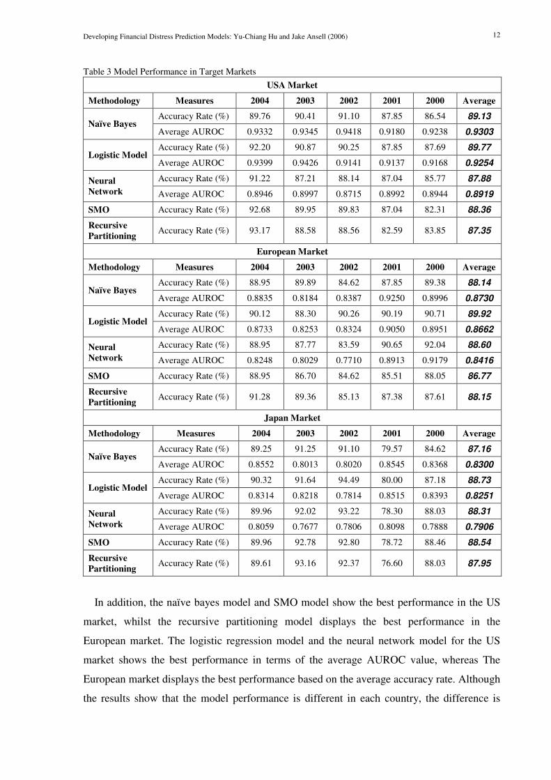
Based on the data in Table 1, an international comparison analysis in terms of both the

accuracy rate and AUROC value can be carried out. Table 3 presents the results in different

countries over 5 years period. It is very obvious that regardless of the target countries, the

average accuracy rates are above 86.5% and the average AUROC values are above 0.79. The

results suggest that the five key variables have sound prediction ability in American,

European and Asian retail markets.


Table 3 Model Performance in Target Markets

USA Market

Methodology Measures 2004 2003 2002 2001 2000 Average

Accuracy Rate (%) 89.76 90.41 91.10 87.85 86.54 89.13 Naïve Bayes

Average AUROC 0.9332 0.9345 0.9418 0.9180 0.9238 0.9303

Accuracy Rate (%) 92.20 90.87 90.25 87.85 87.69 89.77 Logistic Model

Average AUROC 0.9399 0.9426 0.9141 0.9137 0.9168 0.9254

Accuracy Rate (%) 91.22 87.21 88.14 87.04 85.77 87.88 Neural

Network Average AUROC 0.8946 0.8997 0.8715 0.8992 0.8944 0.8919

SMO Accuracy Rate (%) 92.68 89.95 89.83 87.04 82.31 88.36

Recursive

Partitioning Accuracy Rate (%) 93.17 88.58 88.56 82.59 83.85 87.35

European Market



Average AUROC 0.8835 0.8184 0.8387 0.9250 0.8996 0.8730


Average AUROC 0.8733 0.8253 0.8324 0.9050 0.8951 0.8662




Recursive


Japan Market



Average AUROC 0.8552 0.8013 0.8020 0.8545 0.8368 0.8300


Average AUROC 0.8314 0.8218 0.7814 0.8515 0.8393 0.8251




Recursive


In addition, the naïve bayes model and SMO model show the best performance in the US

market, whilst the recursive partitioning model displays the best performance in the

European market. The logistic regression model and the neural network model for the US

market shows the best performance in terms of the average AUROC value, whereas The

European market displays the best performance based on the average accuracy rate. Although

the results show that the model performance is different in each country, the difference is


very small. (The only exception is the performance of neural network model between US and

Japanese markets in terms of the average AUROC value: the difference is around 0.1).

Hence, there is little difference in the models performance.

5.2 Exploring Time Scale

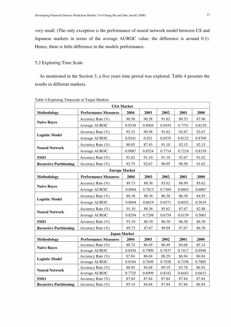
As mentioned in the Section 3, a five years time period was explored. Table 4 presents the

results in different markets.

Table 4 Exploring Timescale in Target Markets

USA Market

Methodology Performance Measures 2004 2003 2002 2001 2000

Accuracy Rate (%) 90.58 90.58 91.62 89.53 87.96 Naïve Bayes

Average AUROC 0.9238 0.8964 0.8454 0.7751 0.8210

Accuracy Rate (%) 92.15 90.58 91.62 92.67 92.67 Logistic Model

Average AUROC 0.9241 0.921 0.8555 0.8123 0.8709

Accuracy Rate (%) 90.05 87.43 91.10 92.15 92.15 Neural Network

Average AUROC 0.9087 0.8524 0.7714 0.7218 0.8339

SMO Accuracy Rate (%) 91.62 91.10 91.10 92.67 91.62

Recursive Partitioning Accuracy Rate (%) 92.75 92.67 90.05 90.58 91.62

Europe Market



Average AUROC 0.8964 0.7813 0.7369 0.6603 0.6067


Average AUROC 0.8694 0.6619 0.6571 0.6052 0.5619


Average AUROC 0.8294 0.7298 0.6754 0.6159 0.5001



Japan Market



Average AUROC 0.8454 0.7909 0.7837 0.7417 0.6948


Average AUROC 0.8184 0.7649 0.7928 0.7358 0.7005


Average AUROC 0.7725 0.6999 0.8342 0.6443 0.6615




The results provide sufficient evidence that for almost all modelling approaches, the model

shows the best performance in the year before financial distress for the target markets. When

comparing US, Europe and Japan market results for each credit scoring approach in 2004, the

differential of results across markets is small. Nevertheless, it is interesting to note that the

US results show the best classification ability for all credit scoring techniques based on both

accuracy rate and AUROC value, except for neural network based on the accuracy rate.

Notwithstanding the small differential across markets the year before financial distress

(2004), it should be said that the longer the period before financial distress, the greater the

difference across markets becomes, especially in terms of AUROC values. For example, five

years prior to financial distress (2000), the US has significantly better AUROC value than

Japan or Europe.

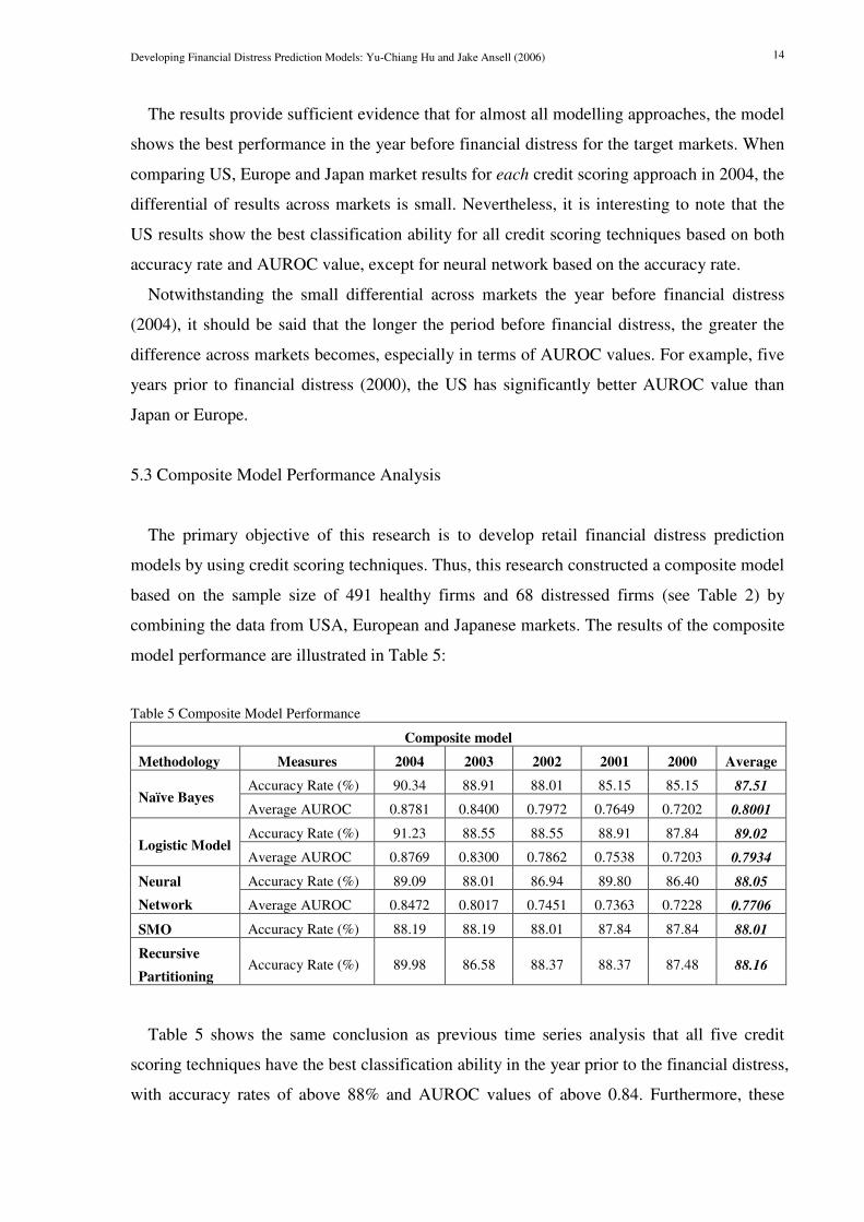
5.3 Composite Model Performance Analysis

The primary objective of this research is to develop retail financial distress prediction

models by using credit scoring techniques. Thus, this research constructed a composite model

based on the sample size of 491 healthy firms and 68 distressed firms (see Table 2) by

combining the data from USA, European and Japanese markets. The results of the composite

model performance are illustrated in Table 5:

Table 5 Composite Model Performance

Composite model



Average AUROC 0.8781 0.8400 0.7972 0.7649 0.7202 0.8001


Average AUROC 0.8769 0.8300 0.7862 0.7538 0.7203 0.7934




Recursive


Table 5 shows the same conclusion as previous time series analysis that all five credit

scoring techniques have the best classification ability in the year prior to the financial distress,

with accuracy rates of above 88% and AUROC values of above 0.84. Furthermore, these


techniques still remain sound five years before financial distress, as the accuracy rate is

above 85% and AUROC value is above 0.72.

With regards to performance of the modelling techniques, the conclusion is the same as Hu

and Ansell (2005) that no modelling methodology has the absolute best classification ability,

since the model’s performance varies in terms of different time scales. For example, logistic

regression model shows the best performance in 2004, but the same cannot be concluded in

different time scales. Furthermore, if we focus on the average performance of each modelling

technique, it is obvious that the performance among five credit scoring approaches is very

similar. (The maximum difference of the average accuracy rate is only 1.5% and the

maximum difference of the AUROC value is only 0.03)

Thus far, the findings above prove that the model has sound discriminating ability, even if

the time period is five years before financial distress. However, due to the sample size limits,

a holdout sample is not likely to employ in this research, and hence, the current results are

potentially overly optimistic. In order to overcome this problem, logistic regression, neural

network and SMO models in the year prior to financial distress are selected for the objective

of credit score ranking comparison with Moody’s credit rating results.

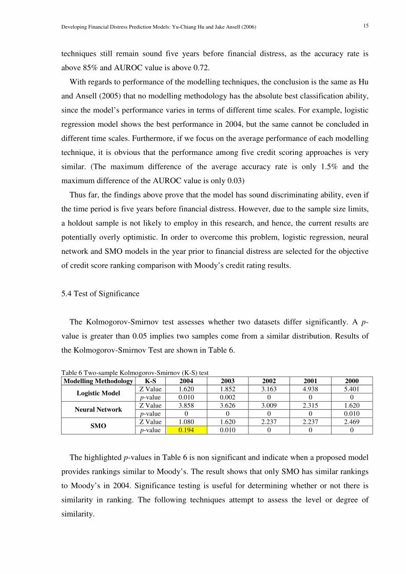
5.4 Test of Significance

The Kolmogorov-Smirnov test assesses whether two datasets differ significantly. A p-

value is greater than 0.05 implies two samples come from a similar distribution. Results of

the Kolmogorov-Smirnov Test are shown in Table 6.

Table 6 Two-sample Kolmogorov-Smirnov (K-S) test

Modelling Methodology K-S 2004 2003 2002 2001 2000

Z Value 1.620 1.852 3.163 4.938 5.401 Logistic Model

p-value 0.010 0.002 0 0 0

Z Value 3.858 3.626 3.009 2.315 1.620 Neural Network

p-value 0 0 0 0 0.010

Z Value 1.080 1.620 2.237 2.237 2.469 SMO

p-value 0.194 0.010 0 0 0

The highlighted p-values in Table 6 is non significant and indicate when a proposed model

provides rankings similar to Moody’s. The result shows that only SMO has similar rankings

to Moody’s in 2004. Significance testing is useful for determining whether or not there is

similarity in ranking. The following techniques attempt to assess the level or degree of

similarity.


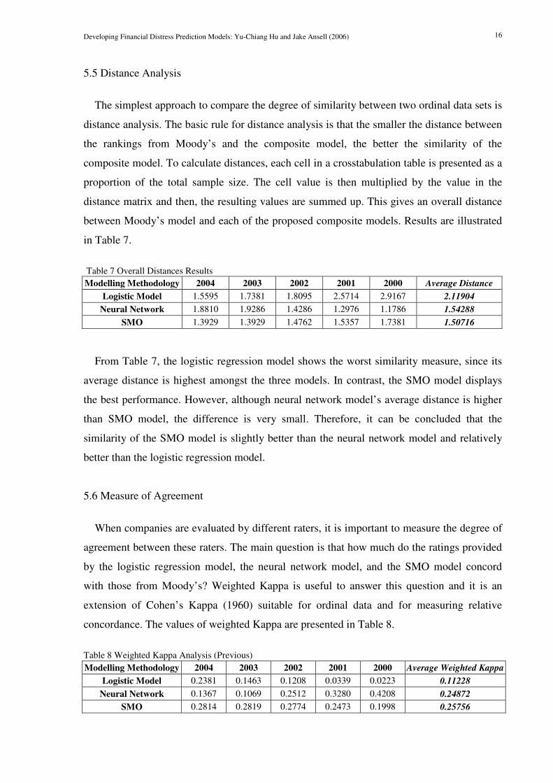
5.5 Distance Analysis

The simplest approach to compare the degree of similarity between two ordinal data sets is

distance analysis. The basic rule for distance analysis is that the smaller the distance between

the rankings from Moody’s and the composite model, the better the similarity of the

composite model. To calculate distances, each cell in a crosstabulation table is presented as a

proportion of the total sample size. The cell value is then multiplied by the value in the

distance matrix and then, the resulting values are summed up. This gives an overall distance

between Moody’s model and each of the proposed composite models. Results are illustrated

in Table 7.

Table 7 Overall Distances Results

Modelling Methodology 2004 2003 2002 2001 2000 Average Distance

Logistic Model 1.5595 1.7381 1.8095 2.5714 2.9167 2.11904

Neural Network 1.8810 1.9286 1.4286 1.2976 1.1786 1.54288

SMO 1.3929 1.3929 1.4762 1.5357 1.7381 1.50716

From Table 7, the logistic regression model shows the worst similarity measure, since its

average distance is highest amongst the three models. In contrast, the SMO model displays

the best performance. However, although neural network model’s average distance is higher

than SMO model, the difference is very small. Therefore, it can be concluded that the

similarity of the SMO model is slightly better than the neural network model and relatively

better than the logistic regression model.

5.6 Measure of Agreement

When companies are evaluated by different raters, it is important to measure the degree of

agreement between these raters. The main question is that how much do the ratings provided

by the logistic regression model, the neural network model, and the SMO model concord

with those from Moody’s? Weighted Kappa is useful to answer this question and it is an

extension of Cohen’s Kappa (1960) suitable for ordinal data and for measuring relative

concordance. The values of weighted Kappa are presented in Table 8.

Table 8 Weighted Kappa Analysis (Previous)

Modelling Methodology 2004 2003 2002 2001 2000 Average Weighted Kappa

Logistic Model 0.2381 0.1463 0.1208 0.0339 0.0223 0.11228

Neural Network 0.1367 0.1069 0.2512 0.3280 0.4208 0.24872

SMO 0.2814 0.2819 0.2774 0.2473 0.1998 0.25756


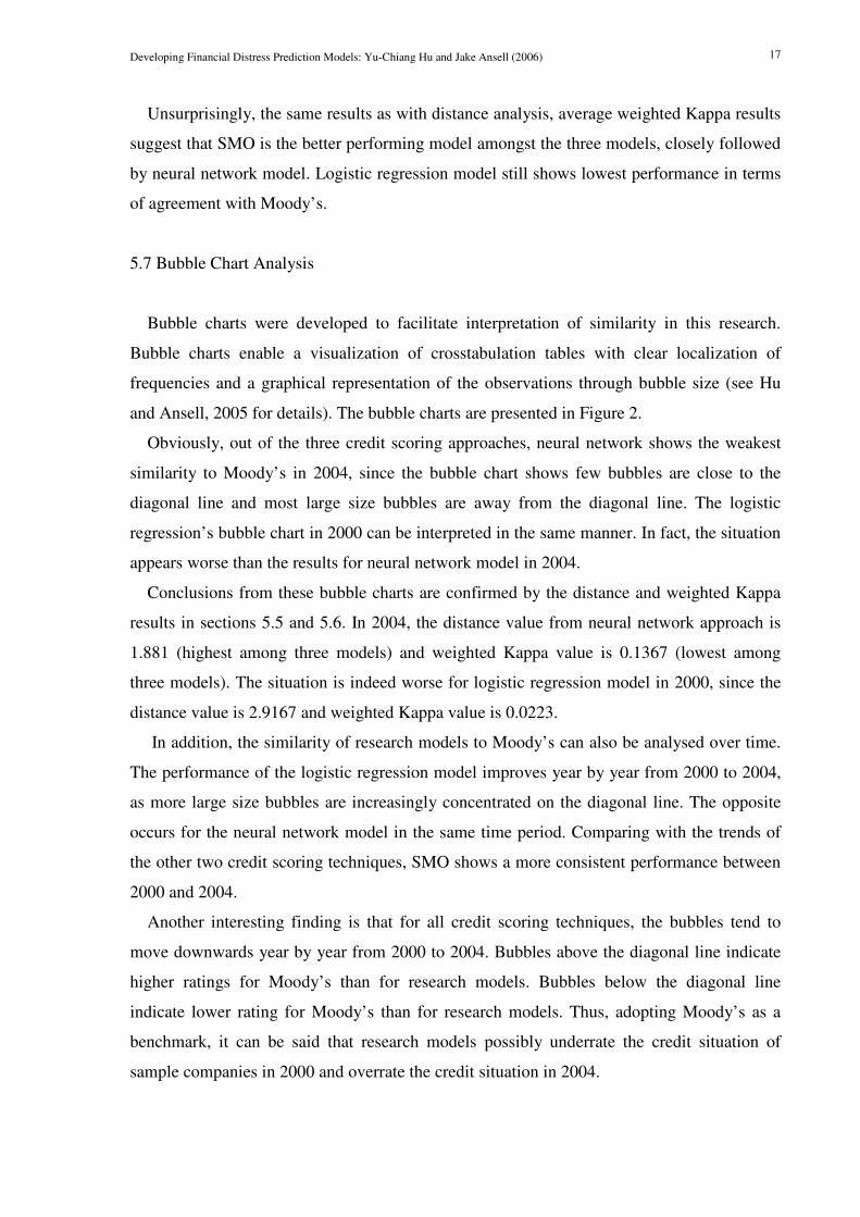
Unsurprisingly, the same results as with distance analysis, average weighted Kappa results

suggest that SMO is the better performing model amongst the three models, closely followed

by neural network model. Logistic regression model still shows lowest performance in terms

of agreement with Moody’s.

5.7 Bubble Chart Analysis

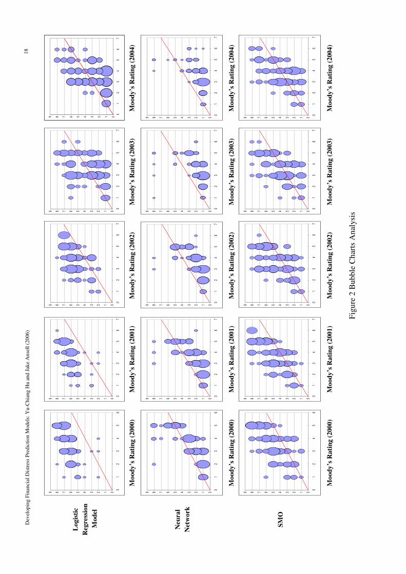
Bubble charts were developed to facilitate interpretation of similarity in this research.

Bubble charts enable a visualization of crosstabulation tables with clear localization of

frequencies and a graphical representation of the observations through bubble size (see Hu

and Ansell, 2005 for details). The bubble charts are presented in Figure 2.

Obviously, out of the three credit scoring approaches, neural network shows the weakest

similarity to Moody’s in 2004, since the bubble chart shows few bubbles are close to the

diagonal line and most large size bubbles are away from the diagonal line. The logistic

regression’s bubble chart in 2000 can be interpreted in the same manner. In fact, the situation

appears worse than the results for neural network model in 2004.

Conclusions from these bubble charts are confirmed by the distance and weighted Kappa

results in sections 5.5 and 5.6. In 2004, the distance value from neural network approach is

1.881 (highest among three models) and weighted Kappa value is 0.1367 (lowest among

three models). The situation is indeed worse for logistic regression model in 2000, since the

distance value is 2.9167 and weighted Kappa value is 0.0223.

In addition, the similarity of research models to Moody’s can also be analysed over time.

The performance of the logistic regression model improves year by year from 2000 to 2004,

as more large size bubbles are increasingly concentrated on the diagonal line. The opposite

occurs for the neural network model in the same time period. Comparing with the trends of

the other two credit scoring techniques, SMO shows a more consistent performance between

2000 and 2004.

Another interesting finding is that for all credit scoring techniques, the bubbles tend to

move downwards year by year from 2000 to 2004. Bubbles above the diagonal line indicate

higher ratings for Moody’s than for research models. Bubbles below the diagonal line

indicate lower rating for Moody’s than for research models. Thus, adopting Moody’s as a

benchmark, it can be said that research models possibly underrate the credit situation of

sample companies in 2000 and overrate the credit situation in 2004.

Dev

elop

ing F

inan

cial

Dis

tres

s P

red

icti

on

Mod

els:

Yu

-Chia

ng H

u a

nd

Jak

e A

nse

ll (

20

06

) 1

8

Lo

gis

tic

Reg

ress

ion

Mo

del

0123456789

01

23

45

6

0123456789

01

23

45

67

0123456789

01

23

45

67

0123456789

01

23

45

67

0123456789

01

23

45

67

M

oo

dy

’s R

ati

ng

(2

00

0)

Mo

od

y’s

Ra

tin

g (

200

1)

Mo

od

y’s

Ra

tin

g (

200

2)

Mo

od

y’s

Ra

tin

g (

200

3)

Mo

od

y’s

Ra

tin

g (

200

4)

Neu

ral

Net

wo

rk

0123456789

01

23

45

6

0123456789

01

23

45

67

0123456789

01

23

45

67

0123456789

01

23

45

67

0123456789

01

23

45

67

M

oo

dy

’s R

ati

ng

(2

00

0)

Mo

od

y’s

Ra

tin

g (

200

1)

Mo

od

y’s

Ra

tin

g (

200

2)

Mo

od

y’s

Ra

tin

g (

200

3)

Mo

od

y’s

Ra

tin

g (

200

4)

SM

O

0123456789

01

23

45

6

0123456789

01

23

45

67

0123456789

01

23

45

67

0123456789

01

23

45

67

0123456789

01

23

45

67

M

oo

dy

’s R

ati

ng

(2

00

0)

Mo

od

y’s

Ra

tin

g (

200

1)

Mo

od

y’s

Ra

tin

g (

200

2)

Mo

od

y’s

Ra

tin

g (

200

3)

Mo

od

y’s

Ra

tin

g (

200

4)

Fig

ure

2 B

ubble

Char

ts A

nal

ysi

s


8. Discussions

This paper constructed a retail financial distress anticipatory model based on five key

variables: Debt Ratio, Total Debt / (Total Debt + Market Capitalization), Total Assets,

Operating Cash Flow and Government Debt / GDP, which proved to have sound

classification performance in Hu and Ansell (2005).

US, European and Japanese markets are chosen for an international comparison analysis

using five credit scoring methodologies, Naïve Bayes, Logistic Regression, Recursive

Partitioning, Artificial Neural Network, and Sequential Minimal Optimization (SMO), over

the time period from 2000 to 2004.

The international comparison analysis shows that regardless of the target countries, the

average accuracy rates are above 86.5% and the average AUROC values are above 0.79.

Moreover, model classification ability is only slightly different in the chosen countries. The

results suggest that the five key variables have sound prediction ability in American,

European and Asian retail markets.

When exploring the time dimension, all three market models possess best prediction

ability in the year prior to financial distress with slight difference across markets. However,

the longer the period before financial distress, the greater the difference across markets

becomes, especially in terms of AUROC values.

The composite model was based on a dataset of 491 healthy and 68 distressed retail firms

from USA, European and Japanese markets, over the time period from 2000 to 2004. Results

show that all five credit-scoring techniques have the best classification ability in the year

prior to the financial distress, with accuracy rates of above 88% and AUROC values of above

0.84. Furthermore, these techniques still remain sound five years before financial distress, as

the accuracy rate is above 85% and AUROC value is above 0.72. However, it is difficult to

conclude which modelling methodology has the absolute best classification ability, since the

model’s performance varies according to different time scales.

The findings above are potentially overly optimistic and may lead to overfitting, due to the

limits of sample size. To overcome this problem, a series of comparison analysis using

Moody’s rating was performed. Based on the Kolmogorov-Smirnov significance test,

distance measure, and weighted Kappa measure, it was found that SMO is the better

performing model amongst the three models, closely followed by neural network model.

Logistic regression model showed lowest performance in terms of similarity with Moody’s.

The bubble chart analysis also proved useful not only for comparing the similarity between


two ordinal datasets, but also for detecting model performance trends. The results displayed

consistent conclusions with other comparison techniques.

Thus far, the conclusions show a paradoxical result in that although the logistic model and

the neural network model display better classification ability than the SMO composite model,

the SMO composite model seems to be stronger in terms of comparability with Moody’s

rankings. A possible explanation is that the logistic regression model and neural network

model fit the sample too closely, hence overfitting, whilst SMO does not.

In comparing the results from the international comparison analysis in this research with

the findings in Hu and Ansell (2005), the performance of the USA model in this paper is

similar to the model ability in Hu and Ansell (2005), despite different time periods. However,

the performance of the European model and the Japanese model is worse than the model in

Hu and Ansell (2005). A possible explanation is that as Hu and Ansell’s (2005) model is

based on the US market, USA model shows better performance than other market models.

Moreover, the ability of the composite model is also worse than Hu and Ansell’s (2005)

model in terms of the AUROC value. This implies that a financial distress model has

potentially better prediction ability when based on a single market. However, model

construction is time-consuming and costly. Hence, global model development is still an

important direction for future research. In this research, the composite model is only based on

US, European and Japanese markets. More world retail markets can be included for future

studies in order to ensure theoretical utility and practical applicability of the financial distress

prediction models.

References

Altman, E.I. (1968) Financial ratios, discriminant analysis and the prediction of corporate

bankruptcy, Journal of Finance, 23, 4, 589-609

Altman, E.I. (1983) Corporate Financial Distress: A Complete Guide to Predicting Avoiding and

Dealing with Bankruptcy, John Wiley and Sons Press, USA

Beaver, W.H. (1966) Financial ratios as predictors of failure, Journal of Accounting Research, 4, 3,

71-111

Betts, J. and Belhoul, D. (1987) The effectiveness of incorporating stability measures in company

failure models, Journal of Business, Finance and Accounting, 14, 3, 323-334

Blum, M. (1974) Failing company discriminant analysis, Journal of Accounting Research, 12, 1,

1-25

Casey, C. and Bartczak, N. (1985) Using operating cash flow data to predict financial distress:

some extensions, Journal of Accounting Research, 23, 1, 384-401


Coats, P.K. and Fant, L.F. (1993) Recognizing financial distress patterns using a neural network

tool, Financial Management, 22, 3, 142-155

Cohen, J. (1960) A coefficient of agreement for nominal scales, Educational and Psychological

Measurement, 20, 37-46.

Dawson, J. (2000) Retailing at century end: some challenges for management and research,

International Review of Retail, Distribution and Consumer Research, 10, 2, 119-148

Deakin, E.B. (1972) A discriminant analysis of predictors of business failure, Journal of

Accounting Research, 10, 1, 167-179

Deakin, E.B. (1976) Distributions of financial accounting ratios: some empirical evidence,

Accounting Review, 51, 1, 90-96

Fan, A. and Palaniswami, M. (2000) Selecting bankruptcy predictors using a support vector

machine approach, Paper presented at 2000 IEEE-INNS-ENNS International Joint Conference on

Neural Networks.

Fitch Ratings (2000) Assigning Credit Ratings to European Retailers, Fitch Ratings Press, USA

(Downloadable from website: http://www.fitchratings.com/)

Fitch Ratings (2001) Corporate: Corporate Rating Methodology, Fitch Ratings Press, New York.

(Downloadable from website http://www.fitchratings.com/)

Frydman, H., Altman, E.l. and Kao, D.L. (1985) Introducing recursive partitioning for financial

classification: the case of financial distress, Journal of Finance, 40, 1, 269-291

Hand, D.J. (1997) Construction and Assessment of Classification Rules, John Wiley & Sons Ltd,

Chichester, UK

Hamer, M. (1983) Failure prediction: Sensitivity of classification accuracy to alternative statistical

methods and variable sets, Journal of Accounting and Public Policy, 2, 189-307

Hosmer, D.W. and Lemeshow, S. (2000) Applied Logistic Regression, Wiley Press, USA

Hu, Y.C., Ansell, J. (2005) Measuring retail company performance by using credit scoring

techniques, submitted to European Journal of Operational Research (EJOR). Paper presented at 2005

Credit Scoring and Credit Control IX, University of Edinburgh, 2005 Paris International Meeting

(French Finance Association) and at 2006 WHU Campus for Finance, Germany

Hunt, S.D. (2000) A General Theory of Competition: Resources, Competences, Productivity,

Economic Growth, Sage Publications Inc., USA

Mar-Molinero, C. and Serrano-Cinca, C. (2001) Bank failure: a multidimensional scaling

approach, European Journal of Finance, 7, 2, 165-183

Marais, M.L., Patell, J.M. and Wolfson, M.A. (1984) The experimental design of classification

models: An application of recursive partitioning and bootstrapping to commercial bank loan

classifications, Journal of Accounting Research, 22 (Supplement), 87-114

McKee, T.E. (2003) Rough sets bankruptcy prediction models versus auditor signalling rates,

Journal of Forecasting, 22, 8, 569-586

Mensah, Y.M. (1983) The differential bankruptcy predictive ability of specific price level

adjustments: some empirical evidence, Accounting Review, 58, 2, 228-246

Mensah, Y.M. (1984) An examination of the stationarity of multivariate bankruptcy prediction

models: A methodological study, Journal of Accounting Research, 22, 1, 380-395

Moody’s Investors Service (1998) Rating Methodology: Industrial Company Rating Methodology,

Moody’s Investors Service Inc. Press, USA (Downloadable from website http://www.moodys.com/)


Moody’s Investors Service (2002) Retail Rating Methodology: Moody’s Approach to Assessing

Key Credit Issues in Retailing, Moody’s Investors Service Inc. Press, USA (Downloadable from

website http://www.moodys.com/)

Moore, A.W. (2001) Cross-validation for detecting and preventing overfitting, Tutorial Slides,

Carnegie Mellon University (Downloadable from website: http://www.cs.cmu.edu/)

Ohlson, J.A. (1980) Financial ratios and the probabilistic prediction of bankruptcy, Journal of

Accounting Research, 18, 1, 109-131

Pantalone, C. and Platt, M. (1987) Predicting failure of savings and loan associations, American

Real Estate and Urban Economics Association Journal, 15, 2, 46-64

Piesse, J. and Wood, D. (1992) Issues in assessing MDA models of corporate failure: a research

note, British Accounting Review, 24, 33-42

Platt, J.C. (1999) Fast Training of Support Vector Machines Using Sequential Minimal

Optimization, In Schölkopf, B., Burges, C.J.C., Smola, A.J. (1999) Advances in Kernel Methods:

Support Vector Machines, MIT press, UK

Platt, H.D. and Platt, M.B. (1990) Development of a class of stable predictive variables, Journal of

Business Finance and Accounting, 17, 1, 31-51

Ross, S.A., Westerfield, R.W. and Jaffe, J. (1999) Corporate Finance, Irwin/McGraw-Hill Press,

USA

Standard and Poor’s (2002) Standard and Poor’s 2002 Corporate Rating Criteria, The McGraw-

Hill Companies press, USA (Downloadable from website: http://www.standardandpoors.com/)

Standard and Poor’s (2003) Standard and Poor’s 2003 Corporate Rating Criteria, The McGraw-

Hill Companies press, USA (Downloadable from website: http://www.standardandpoors.com/)

Standard and Poor’s (2005) Sovereign Risk Indicators: Glossary of Terms, The McGraw-Hill

Companies press, USA (Downloadable from website: http://www.standardandpoors.com/)

Tabachnick, B.G. and Fidel, L.S. (2000) Using Multivariate Statistics, Allyn and Bacon Press, UK

Taffler, R.J. (1982) Forecasting company failure in the UK using discriminant analysis and

financial ratio data, Journal of the Royal Statistical Society, Series A, 145, 3, 342-358

Taffler, R.J. (1984) Empirical models for the monitoring of UK corporations, Journal of Banking

and Finance, 8, 2, 199-227

Tam, K.Y. and Kiang, M.Y. (1992) Managerial applications of neural networks: the case of bank

failure predictions, Management Science, 38, 7, 926-947

Thomas, L.C., Edelman, D.B. and Crook, J.N. (2002) Credit Scoring and Its Applications, Society

for Industrial and Applied Mathematics, Philadelphia, PA.

Trigueiros, D. and Taffler, R. (1996) Neural networks and empirical research in accounting,

Accounting and Business Research, 26, 4, 347-355

Zavgren, C.V. (1983) The prediction of corporate failure: The state of the art, Journal of

Accounting Literature, 2, 1-37

Zhang, G.P., Hu, M.Y., Patuwo, B.E. and Indro, D.C. (1999) Artificial neural networks in

bankruptcy prediction: general framework and cross-validation analysis, European Journal of

Operational Research, 116, 1, 16-32

developing financial distress prediction models 2006/07as-127-developin… · developing financial...

Documents