Determining the Complex Young’s Modulus of Polymer Materials Fabricated

with Microstereolithography

C. Morris*, J. M. Cormack*†, M. F. Hamilton*†, M. R. Haberman*†, C. C. Seepersad*

*Department of Mechanical Engineering, The University of Texas at Austin, Austin, TX 78712

†Applied Research Laboratories, The University of Texas at Austin, Austin, TX 78758

Abstract

Microstereolithography is capable of producing millimeter-scale polymer parts having

micron-scale features. Material properties of the cured polymers can vary depending on build

parameters such as exposure time and laser power. Current techniques for determining the

material properties of these polymers are limited to static measurements via

micro/nanoindentation, leaving the dynamic response undetermined. Frequency-dependent

material parameters, such as the complex Young’s modulus, have been determined for other

relaxing materials by measuring the wave speed and attenuation of an ultrasonic pulse traveling

through the materials. This method is now applied to determine the frequency-dependent

material parameters of polymers manufactured using microstereolithography. Because the

ultrasonic wavelength is comparable to the part size, a model that accounts for both geometric

and viscoelastic effects is used to determine the material properties using experimental data.

Introduction

Parts produced by additive manufacturing (AM) are increasingly utilized for applications

such as energy absorbing honeycomb structures, prosthetic limbs, and shock isolation systems

where the response of the material to dynamic loading must be considered [1, 2, 3]. Due to the

geometric design freedom introduced by AM, parts can achieve mechanical performance levels

previously unattainable by other manufacturing technologies [4]. Successful prediction of the

mechanical performance of parts made from AM processes requires accurate mechanical

modeling which, in turn, requires precise knowledge of rate-dependent material properties of the

as-built parts.

The frequency dependent modulus that relates the stress developed in the material due to

a dynamically applied strain is one such property. The material property describing this

relationship is known as the dynamic modulus, which is frequency dependent and expressed as a

complex quantity that accounts for both storage and loss of mechanical energy. The modulus of

low-loss elastic materials like metals is approximately rate independent for most applications,

and can therefore be described with static elastic moduli. The static Young’s modulus for the

uniaxial loading case is one such property that can be measured through quasi-static tensile or

three point bending tests. If the material exhibits viscoelastic behavior, the mathematical

description of the frequency dependent storage and loss moduli require a more generalized

constitutive model [5], the parameters of which must be obtained experimentally.

When a viscoelastic material is dynamically loaded, some of the imparted strain energy is

stored elastically within the material while some of the energy is dissipated. The amount of

426

Solid Freeform Fabrication 2017: Proceedings of the 28th Annual International Solid Freeform Fabrication Symposium – An Additive Manufacturing Conference

energy that is stored and dissipated can vary with the frequency of the applied load. A general

form of the complex modulus, 𝐸(𝜔), that captures this phenomenon is

𝐸(𝜔) = 𝐸′(𝜔) + 𝑗𝐸′′(𝜔), (1)

where the real part, 𝐸′(𝜔), is the storage modulus corresponding to the frequency-dependent,

elastic storage of energy, and the imaginary part 𝐸′′(𝜔) is the loss modulus that accounts for the

dissipation of dynamic energy. Both the storage and loss modulus must be determined to obtain

the dynamic modulus. However, the standard quasi-static test previously mentioned only

captures the zero frequency component of the storage modulus. In order to obtain the complete

behavior of the dynamic modulus other testing methods must be explored.

One such method, ultrasonic characterization, is of particular interest to the additive

manufacturing community because it is a nondestructive way of measuring dynamic material

properties over a large range of frequencies. It is well documented that the material properties of

parts produced via AM can vary across machines, parts, and even different locations of the same

part [6, 7]. Therefore, a methodology must be developed that can determine material properties

for individual parts both quickly and effectively; furthermore, to be applicable to a range of

processes, including microstereolithography, it must be applicable to parts with small

characteristic dimensions, on the order of millimeters or even smaller. In this paper, an

experimental approach and analysis procedure is applied to determine the dynamic modulus of

an additively manufactured part using ultrasonic characterization. The procedure, in general, can

capture the dynamic modulus for a large range of frequencies, geometries, and part sizes and was

demonstrated on a rod produced by microstereolithography to determine the dynamic modulus in

the ultrasonic range of 400 kHz to 1.3 MHz.

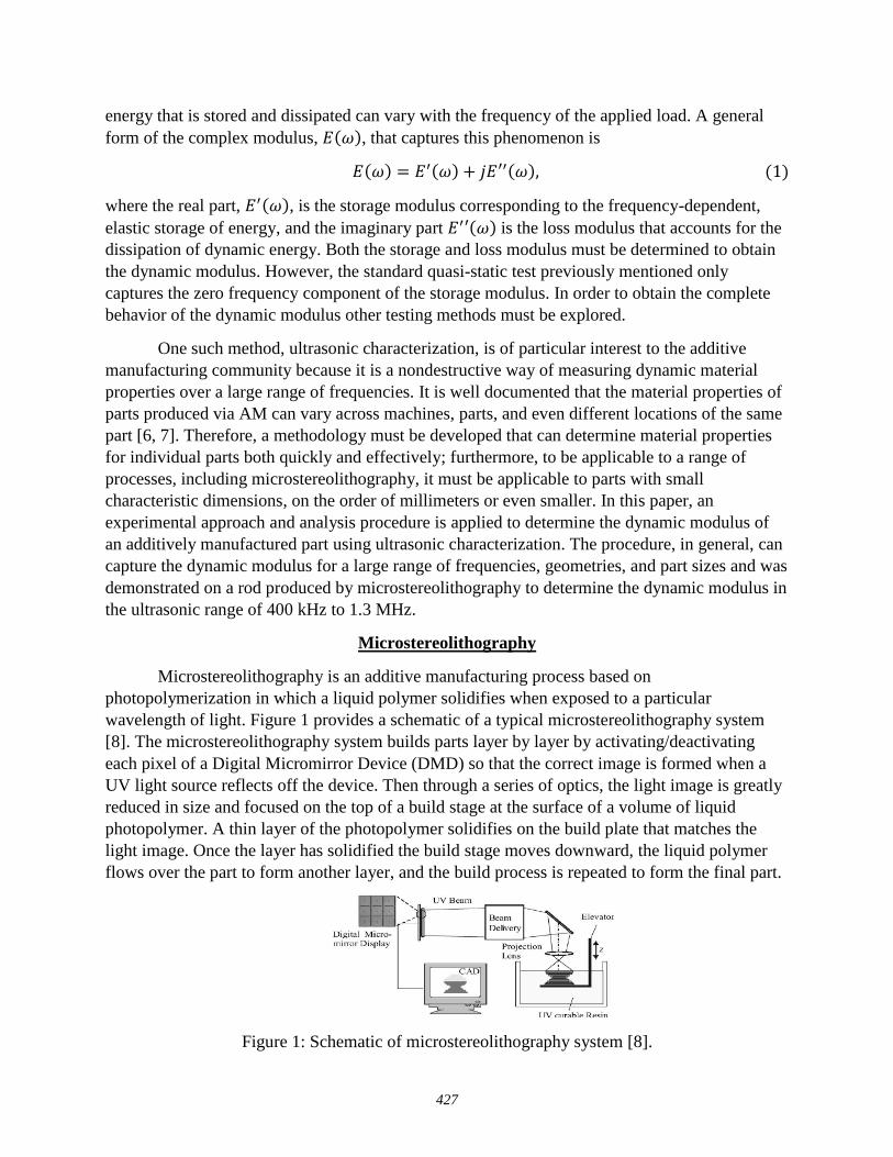
Microstereolithography

Microstereolithography is an additive manufacturing process based on

photopolymerization in which a liquid polymer solidifies when exposed to a particular

wavelength of light. Figure 1 provides a schematic of a typical microstereolithography system

[8]. The microstereolithography system builds parts layer by layer by activating/deactivating

each pixel of a Digital Micromirror Device (DMD) so that the correct image is formed when a

UV light source reflects off the device. Then through a series of optics, the light image is greatly

reduced in size and focused on the top of a build stage at the surface of a volume of liquid

photopolymer. A thin layer of the photopolymer solidifies on the build plate that matches the

light image. Once the layer has solidified the build stage moves downward, the liquid polymer

flows over the part to form another layer, and the build process is repeated to form the final part.

Figure 1: Schematic of microstereolithography system [8].

427

The material properties of the final part produced by microstereolithography will vary

based on several factors including the layer thickness, exposure time, and volume fraction of

constituents [9, 10]. These parameters can vary from build to build based on desired

performance. For example, some builds may require a smaller layer thickness for increased part

resolution. Therefore, a metrology part should be produced for each set of build parameters to

evaluate the dynamic modulus. When developing the metrology part, the build envelope must be

considered because it plays a vital role in determining what testing methods can be used. The

system of interest can produce parts with resolution on the order of tens of microns with overall

parts sizes of about 2.5mm x 2.5mm x 15mm. The resolution and part size can vary from system

to system and the system used in this paper at the University of Akron is capable of the

dimensions previously described. With these geometric constraints, the testing methods to

consider for determining the dynamic modulus are the Impulse Excitation Technique, Dynamic

Mechanical Analysis, Nanoindentation, and ultrasonic material characterization.

Dynamic Modulus Determination

The Impulse Excitation Technique (IET) determines the dynamic modulus by providing

an impulsive load to a sample, which excites the material to vibrate at its natural frequencies

[11]. The quality factor and dynamic modulus can be determined for the material by measuring

the ringdown response, but only at the natural frequencies of the specimen. To obtain the

modulus at other frequencies, multiple specimens must be produced, each having different

geometries that permit the measurement of the dynamic modulus over a wide range of

frequencies. This is rarely an efficient strategy for characterization over wide frequency ranges.

Further, measurement accuracy can be negatively impacted since the material properties of

additively manufactured parts often vary from part to part.

The Dynamic Mechanical Analyzer (DMA) is a commercially available device that can

be used to determine the dynamic modulus of viscoelastic materials [12]. The DMA provides a

time-dependent load to a specimen (usually sinusoidally varying) in a temperature-controlled

environment and measures the response of the part to the load. The DMA then sweeps through

various ambient temperatures to obtain the frequency-dependent response of the material at those

discrete temperatures. The response for all temperature and frequency combinations can then be

used to determine the dynamic modulus of the material for a wide range of frequencies and

temperatures using the principle of time-temperature superposition [13]. This range of

frequencies and temperatures can actually exceed the testable range if the material is

thermorheologically simple, meaning regardless of the initial stress, the stress relaxation times

share the same dependence on changes in temperature [14].

Mixtures of photopolymers and photoinitiators have been shown to be

thermorheologically complex because they exhibit multiple time-temperature shifts from

multiple viscoelastic domains [15]. The principle of time-temperature superposition cannot be

used for these thermorheologically complex materials so the maximum testable frequency of the

DMA bounds the range of attainable information about the dynamic modulus. For commercially

available DMAs this maximum testable frequency is around a few hundred hertz [16].

Furthermore, the DMA requires the specimen to be of a certain geometry to interface with its

428

fixtures. For certain additive manufacturing methods like microstereolithography, it may be

prohibitively difficult to produce a part of adequate size to interface with the provided fixtures,

therefore another testing method is needed to test these parts. It should be noted that Chartrain et

al. used DMA to determine the effect of temperature on the dynamic modulus of a thin film

manufactured by microstereolithography [17]. They were able to produce a viable part because

the build volume of their system was 4mm x 6mm x 35mm which allowed them to produce a

larger test specimen.

Another method, closely related to the DMA is the use of a nanoindentor to deform the

material of interest. Typically, nanoindentation is used to determine the static modulus of

elasticity, but if the machine is carefully calibrated and a sinusoidal indenting force is applied,

the response of the material can be used to determine the frequency-dependent dynamic

modulus. The careful calibration required is an extensive process and, even if carried out to

ASTM standards, the results can differ when compared to the DMA [18]. Similar to the DMA it

also has a limited range of frequencies that can be used to determine the dynamic modulus

limiting the efficacy of the testing.

A method that allows for a large range of frequencies to be evaluated for parts of various

sizes is ultrasonic material characterization. Ultrasonic material characterization measures the

propagation of an input wave pulse in a specimen and relates the response to the material

properties and geometry through a forward model [19]. The forward model is the cornerstone of

the method because it predicts wave propagation through a specimen. Forward models, which

allow the measured response to be inverted to determine material properties, can be constructed

for simple and complex geometries. Therefore, ultrasonic material characterization was selected

as the method to determine the dynamic modulus of the metrology part produced using

microstereolithography.

Before beginning ultrasonic material characterization, a geometry must be selected for

the dynamic modulus metrology part. A natural choice for the design is a cylindrical rod due to

its ability to be produced rapidly by all additive manufacturing technologies. A forward model

for wave propagation in a cylindrical rod is well known and will be discussed in the next section.

Ultrasonic Material Characterization

The simplest definition of ultrasonic material characterization is an experimental method

that uses measurements of the speed of sound in a specimen paired with a forward model to

determine the material properties of the specimen. The forward model relates the frequency-

dependent sound speed to the geometry and frequency-dependent material properties of the

specimen. Accurate measurement of the sound speed paired with knowledge of specimen

geometry can therefore be used to infer the material properties via a minimization of the

difference between the experimental data and forward model predictions as the properties are

varied [20].

The simplest example of ultrasonic material characterization is the determination of a

frequency-independent Young’s modulus of a material by measuring the time-of -flight, or the

time it takes for a wave to travel from one point of a material to another point, in a lossless

429

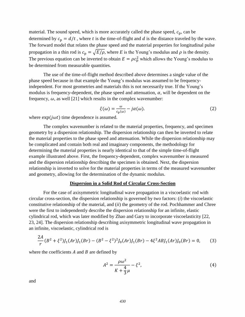
material. The sound speed, which is more accurately called the phase speed, 𝑐p, can be

determined by 𝑐p = 𝑑/𝑡 , where 𝑡 is the time-of-flight and 𝑑 is the distance traveled by the wave.

The forward model that relates the phase speed and the material properties for longitudinal pulse

propagation in a thin rod is 𝑐p = √𝐸/𝜌, where E is the Young’s modulus and 𝜌 is the density.

The previous equation can be inverted to obtain 𝐸 = 𝜌𝑐p2 which allows the Young’s modulus to

be determined from measurable quantities.

The use of the time-of-flight method described above determines a single value of the

phase speed because in that example the Young’s modulus was assumed to be frequency-

independent. For most geometries and materials this is not necessarily true. If the Young’s

modulus is frequency-dependent, the phase speed and attenuation, 𝛼, will be dependent on the

frequency, 𝜔, as well [21] which results in the complex wavenumber:

𝜉(𝜔) =𝜔

𝑐p(𝜔)− 𝑗𝛼(𝜔). (2)

where exp(𝑗𝜔𝑡) time dependence is assumed.

The complex wavenumber is related to the material properties, frequency, and specimen

geometry by a dispersion relationship. The dispersion relationship can then be inverted to relate

the material properties to the phase speed and attenuation. While the dispersion relationship may

be complicated and contain both real and imaginary components, the methodology for

determining the material properties is nearly identical to that of the simple time-of-flight

example illustrated above. First, the frequency-dependent, complex wavenumber is measured

and the dispersion relationship describing the specimen is obtained. Next, the dispersion

relationship is inverted to solve for the material properties in terms of the measured wavenumber

and geometry, allowing for the determination of the dynamic modulus.

Dispersion in a Solid Rod of Circular Cross-Section

For the case of axisymmetric longitudinal wave propagation in a viscoelastic rod with

circular cross-section, the dispersion relationship is governed by two factors: (i) the viscoelastic

constitutive relationship of the material, and (ii) the geometry of the rod. Pochhammer and Chree

were the first to independently describe the dispersion relationship for an infinite, elastic

cylindrical rod, which was later modified by Zhao and Gary to incorporate viscoelasticity [22,

23, 24]. The dispersion relationship describing axisymmetric longitudinal wave propagation in

an infinite, viscoelastic, cylindrical rod is

2𝐴

𝑟(𝐵2 + 𝜉2)𝐽1(𝐴𝑟)𝐽1(𝐵𝑟) − (𝐵2 − 𝜉2)2𝐽0(𝐴𝑟)𝐽1(𝐵𝑟) − 4𝜉2𝐴𝐵𝐽1(𝐴𝑟)𝐽0(𝐵𝑟) = 0, (3)

where the coefficients 𝐴 and 𝐵 are defined by

𝐴2 =𝜌𝜔2

𝐾 +43 𝜇

− 𝜉2, (4)

and

430

𝐵2 =𝜌𝜔2

𝜇− 𝜉2. (5)

In Eq. (3) r is the radius of the rod, 𝐽𝑛(𝑧) is the 𝑛𝑡ℎ order Bessel function of the first kind, K is

the bulk modulus, and 𝜇 is the shear modulus of the material. The bulk modulus and the shear

modulus are related to the Young’s modulus by 𝐸 = 9𝐾𝜇/(3𝐾 + 𝜇) [25]. Note for |𝜉𝑟| ≪ 1 and

as 𝜔 → 0, Eq. (3) reduces to the simple case of longitudinal pulse propagation in a thin rod with

phase speed 𝑐p = √𝐸/𝜌, as discussed in the previous section.

In the derivation of Eq. (3) it is assumed that the rod is infinitely long. In practice then,

the length of the rod, l, must be much larger than the wavelength, λ, where

λ =2𝜋𝑐p

𝜔≪ 𝑙. (6)

Therefore, lower frequency measurements may not be accurately described by Eq. (3), if the

wavelength is on the order of the rod length. This condition must be considered when

investigating rods produced by additive manufacturing systems because the build envelope

determines the maximum rod length. It also should be noted that Eq. (3) cannot be easily

inverted analytically as in the earlier example so that the material properties are given in terms of

the frequency, wavenumber, and geometry. A numerical solver must be used to obtain the

material properties once the other parameters are determined for each frequency. For a given

frequency, there may be multiple solutions to Eq. (3), each corresponding to different modes of

wave propagation along the axis of the rod. The existence of multiple modes requires careful

treatment when measuring the relationship between wavenumber and frequency. Figure 2 shows

equivalent representations of a dispersion plot for an elastic rod where in Figure 2(a) the

horizontal axis is the frequency and the vertical axis is the phase speed and for Figure 2(b) the

horizontal axis is the real component of the wavenumber and the vertical axis is the frequency.

Figure 2: Plot of the (a) phase speed as a function of frequency and (b) the real component of

inverse wavelength as a function of frequency when multiple modes are present for r = 1.25 mm,

E = 4.5 GPa, and ν = 0.375.

431

As shown in Figure 2, when a cylindrical rod is excited, multiple modes may propagate

through the rod and appear in the complex wavenumber measurement. The following section

discusses how this measurement of the complex wavenumber is performed

Determining Complex Wavenumber

Determining the complex wavenumber requires measuring both the frequency-dependent

phase speed and wave attenuation. This is accomplished by measuring ultrasonic wave packets at

a range of positions as they propagate along the axis of the rod to obtain spatial and temporal

information about the propagating wave. Performing a two-dimensional (2D) fast Fourier

transform (FFT), with one dimension being time and the other space, one obtains the complex

amplitude of the propagating pulses for frequency, wavenumber pairs. The data is easily

visualized with a surface plot where the horizontal axis is the real component of the

wavenumber, the vertical axis is the frequency, and the magnitude is the amplitude of the

transformed signal. This representation is commonly referred to as the dispersion diagram of the

elastic waveguide. If only axisymmetric modes are present, the amplitude of the surface plot is

dramatically higher along curves that satisfy the dispersion relationship Eq. (3). The degree of

agreement between the values calculated with Eq. (3) (the forward model) and the experimental

data depends primarily on the accuracy of the material properties provided as inputs to the

forward model. As previously discussed, multiple modes may be present, so filtering of the data

may be required if one wishes to isolate any specific propagating mode. Once a single mode is

isolated from the dispersion diagram, the frequency-dependent phase speed for the mode of

interest can be extracted by determining the real component of the wave number for each

frequency where the amplitude of the signal is highest. This allows for numerical determination

of the phase speed.

With the isolated mode, it is then possible to use the filtered data to determine the

imaginary component of the wavenumber. An inverse Fourier transform of the filtered data can

be taken to yield the amplitude of the selected mode in time and space. For each measurement

separated by a distance Δ𝑥, a FFT can be taken in the time domain. Then the transfer

function 𝐻(𝜔) between adjacent measurements, �̃�2(𝜔, 𝑥) and �̃�1(𝜔, 𝑥), is defined to be

𝐻(𝜔) =�̃�2

�̃�1

= 𝑒−𝛼Δ𝑥𝑒−

𝑗𝜔𝑐𝑝

Δ𝑥. (7)

The magnitude of the transfer function and knowledge of distance between measurement

locations can then be used to determine the attenuation coefficient using the expression

𝛼 = −1

Δxln|𝐻(𝜔)|. (8)

The method described above provides a means to determine the real and imaginary components

of the complex wavenumber from experimentally obtained data. That information is then used to

determine the material properties through inversion of the dispersion relationship Eq. (3).

The complex wavenumber can be constructed at each frequency where attenuation and

phase speed information is available through Eq. (2). The complex wavenumber and frequency

432

are substituted into the dispersion relationship of Eq. (3) which is then separated into its real and

imaginary components forming a system of two simultaneous equations. The material properties

are then determined by obtaining values of the bulk modulus and shear modulus that minimize

the magnitude of both equations through the use of the fsolve function in MATLAB®. This

methodology was applied to a rod produced via microstereolithography. The experimental setup

and results are discussed in the next section.

Experimental Setup and Results

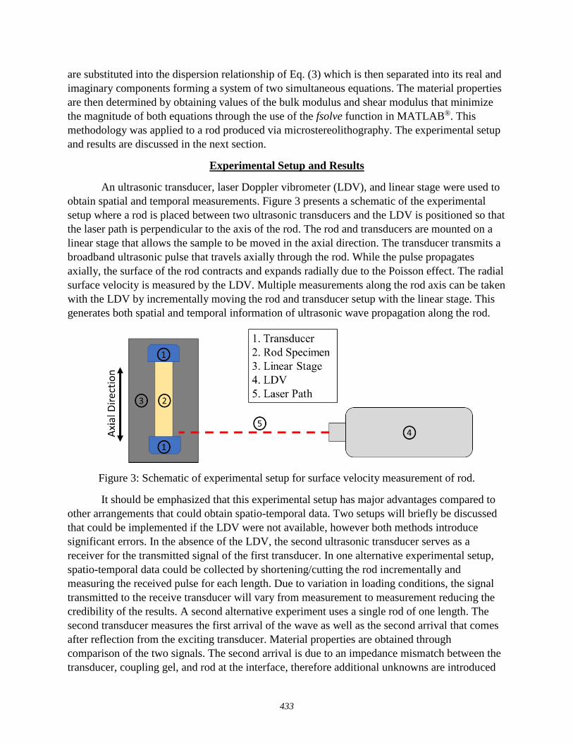
An ultrasonic transducer, laser Doppler vibrometer (LDV), and linear stage were used to

obtain spatial and temporal measurements. Figure 3 presents a schematic of the experimental

setup where a rod is placed between two ultrasonic transducers and the LDV is positioned so that

the laser path is perpendicular to the axis of the rod. The rod and transducers are mounted on a

linear stage that allows the sample to be moved in the axial direction. The transducer transmits a

broadband ultrasonic pulse that travels axially through the rod. While the pulse propagates

axially, the surface of the rod contracts and expands radially due to the Poisson effect. The radial

surface velocity is measured by the LDV. Multiple measurements along the rod axis can be taken

with the LDV by incrementally moving the rod and transducer setup with the linear stage. This

generates both spatial and temporal information of ultrasonic wave propagation along the rod.

Figure 3: Schematic of experimental setup for surface velocity measurement of rod.

It should be emphasized that this experimental setup has major advantages compared to

other arrangements that could obtain spatio-temporal data. Two setups will briefly be discussed

that could be implemented if the LDV were not available, however both methods introduce

significant errors. In the absence of the LDV, the second ultrasonic transducer serves as a

receiver for the transmitted signal of the first transducer. In one alternative experimental setup,

spatio-temporal data could be collected by shortening/cutting the rod incrementally and

measuring the received pulse for each length. Due to variation in loading conditions, the signal

transmitted to the receive transducer will vary from measurement to measurement reducing the

credibility of the results. A second alternative experiment uses a single rod of one length. The

second transducer measures the first arrival of the wave as well as the second arrival that comes

after reflection from the exciting transducer. Material properties are obtained through

comparison of the two signals. The second arrival is due to an impedance mismatch between the

transducer, coupling gel, and rod at the interface, therefore additional unknowns are introduced

433

to the measurement. Furthermore, if the material attenuates strongly, the signal from the reflected

signal will be too small to detect. For viscoelastic rods, like the ones selected, the reflected signal

is far too weak to be measured above the noise level.

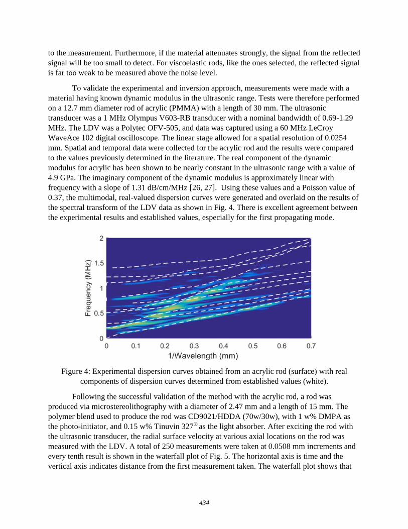
To validate the experimental and inversion approach, measurements were made with a

material having known dynamic modulus in the ultrasonic range. Tests were therefore performed

on a 12.7 mm diameter rod of acrylic (PMMA) with a length of 30 mm. The ultrasonic

transducer was a 1 MHz Olympus V603-RB transducer with a nominal bandwidth of 0.69-1.29

MHz. The LDV was a Polytec OFV-505, and data was captured using a 60 MHz LeCroy

WaveAce 102 digital oscilloscope. The linear stage allowed for a spatial resolution of 0.0254

mm. Spatial and temporal data were collected for the acrylic rod and the results were compared

to the values previously determined in the literature. The real component of the dynamic

modulus for acrylic has been shown to be nearly constant in the ultrasonic range with a value of

4.9 GPa. The imaginary component of the dynamic modulus is approximately linear with

frequency with a slope of 1.31 dB/cm/MHz [26, 27]. Using these values and a Poisson value of

0.37, the multimodal, real-valued dispersion curves were generated and overlaid on the results of

the spectral transform of the LDV data as shown in Fig. 4. There is excellent agreement between

the experimental results and established values, especially for the first propagating mode.

Figure 4: Experimental dispersion curves obtained from an acrylic rod (surface) with real

components of dispersion curves determined from established values (white).

Following the successful validation of the method with the acrylic rod, a rod was

produced via microstereolithography with a diameter of 2.47 mm and a length of 15 mm. The

polymer blend used to produce the rod was CD9021/HDDA (70w/30w), with 1 w% DMPA as

the photo-initiator, and 0.15 w% Tinuvin 327® as the light absorber. After exciting the rod with

the ultrasonic transducer, the radial surface velocity at various axial locations on the rod was

measured with the LDV. A total of 250 measurements were taken at 0.0508 mm increments and

every tenth result is shown in the waterfall plot of Fig. 5. The horizontal axis is time and the

vertical axis indicates distance from the first measurement taken. The waterfall plot shows that

434

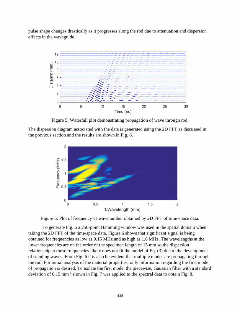
pulse shape changes drastically as it progresses along the rod due to attenuation and dispersion

effects in the waveguide.

Figure 5: Waterfall plot demonstrating propagation of wave through rod.

The dispersion diagram associated with the data is generated using the 2D FFT as discussed in

the previous section and the results are shown in Fig. 6.

Figure 6: Plot of frequency vs wavenumber obtained by 2D FFT of time-space data.

To generate Fig. 6 a 250-point Hamming window was used in the spatial domain when

taking the 2D FFT of the time-space data. Figure 6 shows that significant signal is being

obtained for frequencies as low as 0.15 MHz and as high as 1.6 MHz. The wavelengths at the

lower frequencies are on the order of the specimen length of 15 mm so the dispersion

relationship at those frequencies likely does not fit the model of Eq. (3) due to the development

of standing waves. From Fig. 6 it is also be evident that multiple modes are propagating through

the rod. For initial analysis of the material properties, only information regarding the first mode

of propagation is desired. To isolate the first mode, the piecewise, Gaussian filter with a standard

deviation of 0.15 mm-1 shown in Fig. 7 was applied to the spectral data to obtain Fig. 8.

435

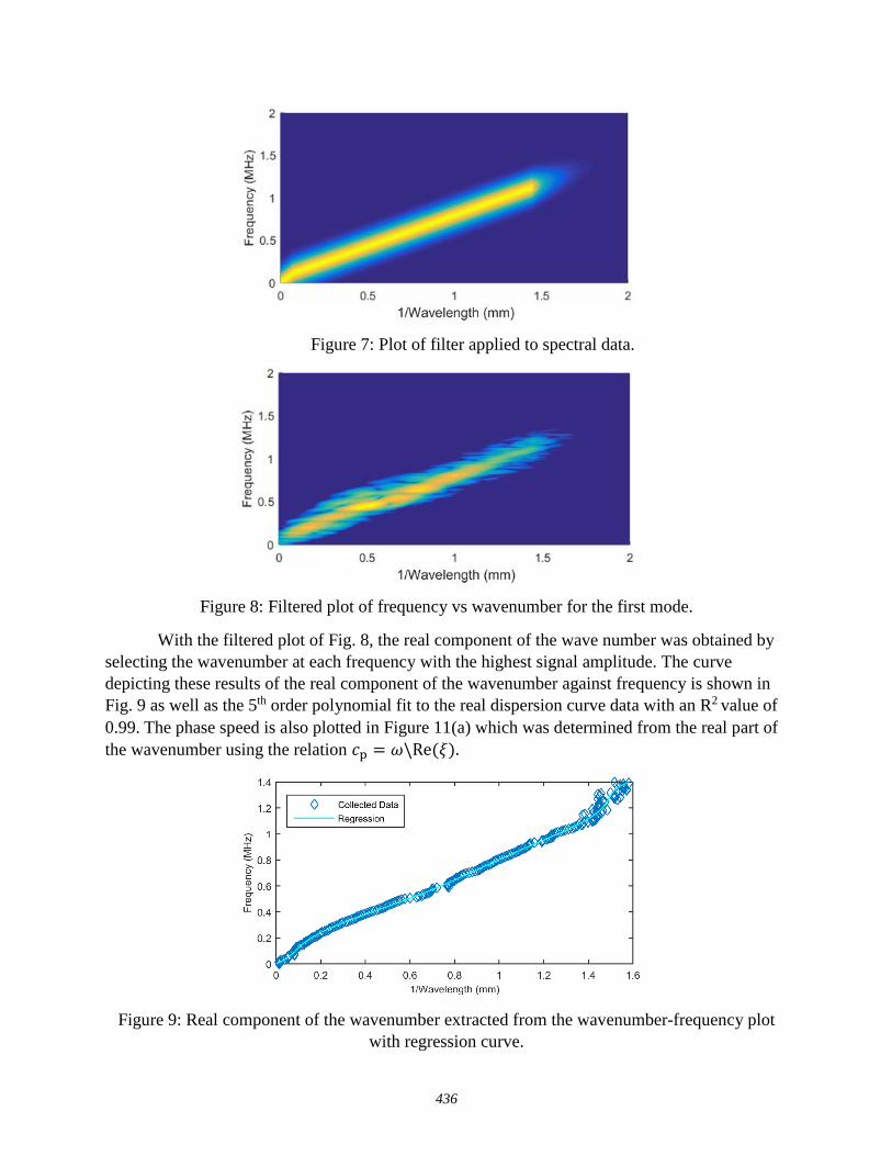
Figure 7: Plot of filter applied to spectral data.

Figure 8: Filtered plot of frequency vs wavenumber for the first mode.

With the filtered plot of Fig. 8, the real component of the wave number was obtained by

selecting the wavenumber at each frequency with the highest signal amplitude. The curve

depicting these results of the real component of the wavenumber against frequency is shown in

Fig. 9 as well as the 5th order polynomial fit to the real dispersion curve data with an R2 value of

0.99. The phase speed is also plotted in Figure 11(a) which was determined from the real part of

the wavenumber using the relation 𝑐p = 𝜔\Re(𝜉).

Figure 9: Real component of the wavenumber extracted from the wavenumber-frequency plot

with regression curve.

436

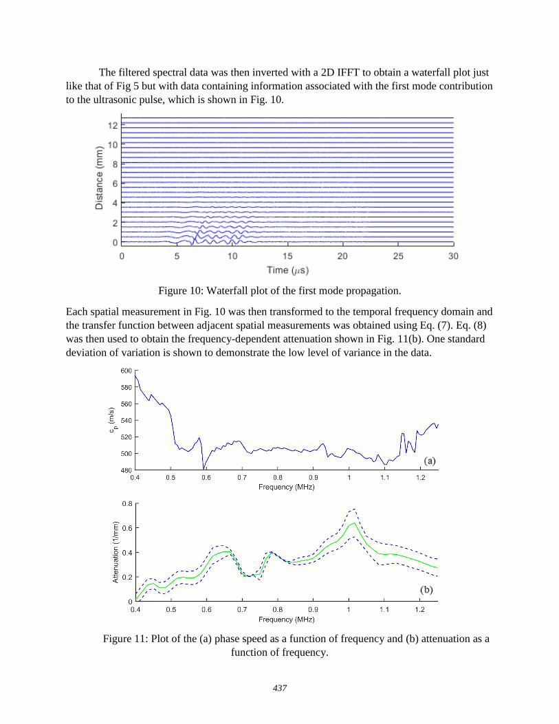
The filtered spectral data was then inverted with a 2D IFFT to obtain a waterfall plot just

like that of Fig 5 but with data containing information associated with the first mode contribution

to the ultrasonic pulse, which is shown in Fig. 10.

Figure 10: Waterfall plot of the first mode propagation.

Each spatial measurement in Fig. 10 was then transformed to the temporal frequency domain and

the transfer function between adjacent spatial measurements was obtained using Eq. (7). Eq. (8)

was then used to obtain the frequency-dependent attenuation shown in Fig. 11(b). One standard

deviation of variation is shown to demonstrate the low level of variance in the data.

Figure 11: Plot of the (a) phase speed as a function of frequency and (b) attenuation as a

function of frequency.

437

The attenuation of the material is characteristic of a viscoelastic material where the

attenuation, in general, increases with frequency. With the real and imaginary components of the

wavenumber determined, the dynamic modulus was determined by inverting the dispersion

relation Eq. (3) and assuming a Poisson ratio of 0.375. Results are presented in Fig. 12 where the

variation in the dynamic modulus, plotted in green, is derived from the variation in the

attenuation and the blue line is determined with the mean attenuation values.

Figure 12: Plot of the (a) real component of dynamic modulus and (b) imaginary component of

dynamic modulus.

The dynamic modulus was obtained for the frequency range of 0.4 MHz to 1.3 MHz

although there was information outside this range. This range was chosen to match the nominal

bandwidth of the transducer as well as to ensure the assumptions regarding the dispersion

relationship were not violated. The values of the moduli are well within reasonable limits as the

static modulus for both HDDA and CD9021 have been both experimentally determined to be

around 1 GPa [28, 29].

To corroborate the value of the storage modulus of 0.59 MPa at 400 kHz that was

determined through ultrasonic material characterization, a secondary experiment was designed to

measure the storage modulus at lower frequencies. The experimental setup is shown in Figure 13

438

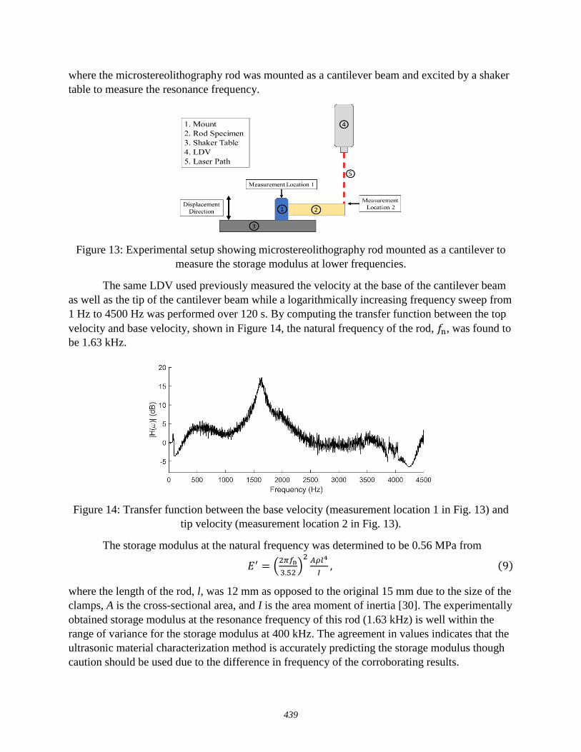
where the microstereolithography rod was mounted as a cantilever beam and excited by a shaker

table to measure the resonance frequency.

Figure 13: Experimental setup showing microstereolithography rod mounted as a cantilever to

measure the storage modulus at lower frequencies.

The same LDV used previously measured the velocity at the base of the cantilever beam

as well as the tip of the cantilever beam while a logarithmically increasing frequency sweep from

1 Hz to 4500 Hz was performed over 120 s. By computing the transfer function between the top

velocity and base velocity, shown in Figure 14, the natural frequency of the rod, 𝑓n, was found to

be 1.63 kHz.

Figure 14: Transfer function between the base velocity (measurement location 1 in Fig. 13) and

tip velocity (measurement location 2 in Fig. 13).

The storage modulus at the natural frequency was determined to be 0.56 MPa from

𝐸′ = (2𝜋𝑓n

3.52)

2 𝐴𝜌𝑙4

𝐼, (9)

where the length of the rod, l, was 12 mm as opposed to the original 15 mm due to the size of the

clamps, A is the cross-sectional area, and I is the area moment of inertia [30]. The experimentally

obtained storage modulus at the resonance frequency of this rod (1.63 kHz) is well within the

range of variance for the storage modulus at 400 kHz. The agreement in values indicates that the

ultrasonic material characterization method is accurately predicting the storage modulus though

caution should be used due to the difference in frequency of the corroborating results.

439

Conclusion

A methodology for determining the dynamic modulus of parts produced by additive

manufacturing was applied to a rod produced by microstereolithography. By modeling the

dispersion relationship for the part of interest and then measuring the frequency-dependent

attenuation and sound speed experimentally, the dynamic modulus was determined. For the

microstereolithography rod, the dynamic modulus was obtained in the ultrasonic range of 0.4

MHz -1.3 MHz by utilizing the dispersion relationship for an infinite cylindrical rod. This range

of frequencies is much larger than that of most methods to determine the dynamic modulus and

quasi-static modulus like DMA, IET, and nanoindentation.

Future work will focus on obtaining the dynamic modulus at higher and lower

frequencies than those already determined. Determination of the modulus at lower frequencies

while simultaneously obtaining a wide frequency range of dynamic moduli can be accomplished

by using a longer rod length or different dispersion relationship. To increase the upper limit on

the frequency range, information regarding higher mode wave propagation can be explored.

Acknowledgements

The authors would like to acknowledge support from the National Science Foundation

under Grant No. CMMI -1435548. We would also like to acknowledge Sumanth Kashyap and

Dr. Jae-Won Choi from the University of Akron and Dr. Eric MacDonald from Youngstown

State for their input and production of the microstereolithography rods. Any opinions, findings

and conclusions or recommendations expressed in this material are those of the authors and do

not necessarily reflect the views of the sponsor.

440

References

[1] D. M. Correa, T. Klatt, S. Cortes, M. R. Haberman, D. Kovar and C. C. Seepersad,

"Negative Stiffness Honeycombs for Recoverable Shock Isolation," Rapid Prototyping

Journal, vol. 21, no. 2, pp. 193-200, 2015.

[2] N. P. Fey, G. K. Klute and R. R. Neptune, "The Influence of Energy Storage and Return

Foot Stiffness on Walking Mechanics and Muscle activity in Below-Knee Amputees,"

Clinical Biomechanics, vol. 26, no. 10, pp. 1025-1032, 2011.

[3] B. A. Fulcher, D. W. Shahan, M. R. Haberman, C. C. Seepersad and P. S. Wilson,

"Analytical and Experimental Investigation of Buckled Beams as Negative Stiffness

Elements for Passive Vibration and Shock Isolation Systems," Journal of Vibration and

Acoustics, vol. 136, no. 3, p. 031009, 2014.

[4] B. Derby, "Printing and Prototyping of Tissues and Scaffolds," Science, vol. 338, no. 6109,

pp. 921-926, 2012.

[5] H. T. Banks, S. Hu and Z. R. Kenz, "A Brief Review of Elasticity and Viscoelasticity for

Solids," Advances in Applied Mathematics and Mechanics, vol. 3, no. 1, pp. 1-51, 2011.

[6] D. L. Bourell, T. J. Watt, D. K. Leigh and B. Fulcher, "Performance Limitation in Polymer

Laser Sintering," Physics Procedia, vol. 56, pp. 147-156, 2014.

[7] W. W. Wroe, "Improvements and Effects of Thermal History on Mechanical Properties for

Polymer Selective Laser Sintering (SLS)," Master's Thesis, Univ. of Texas at Austin, 2015.

[8] C. Sun, N. Fang, D. M. Wu and X. Zhang, "Projection Micro-Stereolithography Using

Digital Micro-Mirror Dynamic Mask," Sensors and Actuators, vol. 121, no. 1, pp. 113-120,

2005.

[9] J. M. Dulieu-Barton and M. C. Fulton, "Mechanical Properties of a Typical

Microstereolithography Resin," Strain, vol. 36, no. 2, pp. 81-87, 2000.

[10] K. Chockalingam, N. Jawahar and U. Chandrasekhar, "Influence of Layer Thickness on

Mechanical Properties in Stereolithography," Rapid Prototypinc Journal, vol. 12, no. 2, pp.

106-113, 2006.

[11] G. Roebben, B. Bollen, A. Brebels, J. Van Humbeeck and O. Van der Biest, "Impulse

Excitiation Apparatus to Measure Resonant Frequinces, Elastic Modulis, and Internal

Friction at Room and HIgh Temperature," Review of Scientific Instruments, vol. 68, no. 12,

pp. 4511-4515, 1997.

[12] N. G. McCrum, B. E. Read and W. Graham, Anelastic and Dielectric Effects in Polymeric

Solids, Wiley,New York: Dover, 1967.

441

[13] M. L. Williams, R. F. Landel and J. D. Ferry, "The Temperature Dependence of Relaxation

Mechanisms in Amorphous Polymers and Other Glass-forming Liquids," Journal of the

American Chemical Society, vol. 77, no. 14, pp. 3701-3707, 1955.

[14] J. D. Ferry, Viscoelastic Properties of Polymers, New York: John Wiley & Sons, 1980.

[15] P. M. Johnson and C. M. Stafford, "Surface Indentation Arrays for High-thoroughput

Analysis of Viscoelastic Material Properties," in Review of Scientific Instruments, 2009.

[16] TA Instruments, "Dynamic Mechanical Analyzer: Q Series, Getting Started Guide," New

Castle, Delaware, 2004.

[17] N. A. Chartrain, M. Vratsanos, D. T. Han, J. M. Sirrine, A. Pekkanen, T. E. Long, A. R.

Whittington and C. B. Williams, "Microstereolithography of Tissue Scaffolds Using a

Biodegradable Photocurable Polyester," in Solid Freeform Fabrication Sympossium,

Austin, Texas, 2016.

[18] E. G. Herbert, W. C. Oliver and G. M. Pharr, "Nanoindentation and the Dynamic

Characterization of Viscoelastic Solids," Journal of Phyics D: Applied Physics, vol. 41, no.

7, p. 074021, 2008.

[19] F. A. Firestone, "Flaw Detecting Device and Measuring Instrument". US Patent 2,280,226,

21 April 1942.

[20] D. E. Chimenti and A. H. Nayfeh, "Ultrasonic Reflection and Guided Wave Propagation in

Biaxially Laminated Composite Plates," The Journal of the Acoustical Society of America,

vol. 87, no. 4, pp. 1409-1415, 1990.

[21] M. O'Donnell, E. T. Jaynes and J. G. Miller, "Kramers-Kronig Relationship Between

Ultrasonic Attenuation and Phase Velocity," The Journal of the Acoustical Society of

America, vol. 69, no. 3, pp. 696-701, 1981.

[22] C. Chree, "The Equations of an Isotropic Elastic Solid in Polar and Cylindrical Co-

ordinates their Solution and Application," Transactions of the Cambridge Philosophical

Society, vol. 14, p. 250, 1889.

[23] L. Pochhammer, "Ueber Die Fortpflanzungsgeschwindigkeiten Kleiner Schwingungen in

Einem Unbegrenzten Isotropen Kreiscylinder," Journal für die reine und angewandte

Mathematik, vol. 81, pp. 324-336, 1876.

[24] H. Zhao and G. Gary, "A Three DImensional Analytical Solution of the Longitudinal Wave

Propagation in an Infinite Linear Viscoelastic Cylindrical Bar. Application to Experimental

Techniques," J. Mech. Phys. Solids, vol. 43, no. 8, pp. 1335-1348, 1995.

442

[25] M. H. Sadd, Elasticity: Theory, Applications, and Numerics, Kidlington, Oxford: Elsevier,

2014.

[26] P. E. Bloomfield, W.-J. Lo and P. A. Lewin, "Experimental Study of the Acoustical

Properties of Polymers Utilized to Construct PVDF Ultrasonic Transducers and the

Acousto-Electric Properties of PVDF and P(VDF/TrFE) Films," IEEE transactions on

Ultrasonics, Ferroelectrics, and Frequency Control, vol. 47, no. 6, pp. 1397-1405, 2000.

[27] J. L. Williams and W. J. H. Johnson, "Elastic Constants of Composites Formed from

PMMA Bone Cement and Anisotropic Bovine Tibial Cancellous Bone," J. Biomechanics,

vol. 22, no. 6/7, pp. 673-682, 1989.

[28] X. Zheng, H. Lee, T. H. Weisgraber, M. Shusteff, J. DeOtte, E. B. Duoss, J. D. Kuntz, M.

M. Biener, Q. Ge, J. A. Jackson, S. O. Kucheyev, N. X. Fang and C. M. Spadaccini,

"Ultralight, Ultrastiff Mechanical Metamaterials," Science, vol. 344, no. 6190, pp. 1373-

1377, 2014.

[29] A. Olivier, L. Benkhaled, T. Pakula, B. Ewen, A. Best, M. Benmouna and U. Maschke,

"Static and Dynamic Mechanical Behavior of Electron Beam-Beam Cured Monomer and

Monomer/Liquid Crystal Systems," Macromolecular Materials and Engineering, vol. 289,

no. 12, pp. 1047-1052, 2004.

[30] W. C. Young, R. G. Budynas and A. M. Sadegh, Roark's Formulas for Stress and Strain,

New York: McGraw-Hill, 2011.

443