Determining Energy Expenditure from TreadmillWalking using Hip-Worn Inertial Sensors:

An Experimental StudyHarshvardhan Vathsangam, Adar Emken, E. Todd Schroeder, Donna Spruijt-Metz and Gaurav S. Sukhatme

Abstract—We describe an experimental study to estimateenergy expenditure during treadmill walking using a singlehip-mounted inertial sensor ( triaxial accelerometer and triax-ial gyroscope). Typical physical activity characterization usingcommercial monitors use proprietary counts that do not havea physically interpretable meaning. This paper emphasizes therole of probabilistic techniques in conjunction with inertialdata modeling to accurately predict energy expenditure forsteady-state treadmill walking. We represent the cyclic natureof walking with a Fourier transform and show how to map thisrepresentation to energy expenditure (V O2, mL/min) using threeregression techniques. A comparative analysis of the accuracyof sensor streams in predicting energy expenditure reveals thatusing triaxial information leads to more accurate energy expen-diture prediction compared to only using one axis. Combiningaccelerometer and gyroscopic information leads to improvedaccuracy compared to using either sensor alone. Nonlinearregression methods showed better prediction accuracy comparedto linear methods but required an order of higher magnitude ofrun time.

Index Terms—Accelerometer, Energy expenditure, Gyroscope,Treadmill walking

I. INTRODUCTION

Physical inactivity is the fourth leading risk factor forglobal mortality (6% of global deaths) and is estimated tobe the main cause of approximately 21–25% of breast andcolon cancers, 27% of diabetes and approximately 30% ofischaemic heart disease burden [1]. Regular physical activityis known to reduce obesity, risks for cardiovascular disease,type 2 diabetes, and several forms of cancer [2]. In thequest to promote healthier lifestyles, technological solutionsprovide users and clinicians with objective measures of activityintensity that can be used in feedback and interventions. Thechallenge is to provide these tools in real-time and in portableform.

In recent years, considerable research has been directedtowards the detection and classification of physical activitypatterns from body mounted kinematic sensors [3]. Inertialsensors capture movement either by measuring body acceler-ations (accelerometers) or rotational rates (gyroscopes). Dueto their small size, low cost, increasingly high precision, low

Revised version submitted April 30, 2011.This work was supported in part by Qualcomm, Nokia, NSF (CCR-

0120778) as part of the Center for Embedded Network Sensing (CENS), andthe USC Comprehensive NCMHD Research Center of Excellence (P60 MD002254). Support for H. Vathsangam was provided by the USC AnnenbergDoctoral fellowship program.

H. Vathsangam and G. S. Sukhatme are with the Department of ComputerScience, University of Southern California, Los Angeles, CA 90089. vathsang| gaurav @ usc.edu

A. Emken and D. Spruijt-Metz are with the Department of PreventiveMedicine, University of Southern California, Los Angeles, CA 90089. emken| dmetz @ usc.edu

E.T. Schroeder is with the Division of Biokinesiology and Physical Therapy,University of Southern California, Los Angeles, CA 90089. eschroed@usc.edu

power consumption and portability, inertial sensors are anattractive option for deriving relevant physiological quantitiesfrom human movement [4].

Energy expenditure prediction in walking: Walking is aneasy and common activity that can be used to maintain anactive lifestyle [5]. An objective measure of the intensity ofwalk is the energy expended. An immediate question to ask iswhether body-worn inertial measurements can be exploited topredict energy expenditure. Can these predictions be improvedwith sophisticated analytical techniques? Finally, which kindsand combonations of sensors are better at predicting energyexpenditure?

The domain: Here, we address the problem of estimatingenergy expenditure using body-mounted inertial sensors for aparticular activity: treadmill walking. Treadmill walking waschosen because it allows the capture of a regular, well-definedand easily quantifiable movement in a laboratory setting. Weuse inertial data from a triaxial accelerometer and triaxialgyroscope mounted on the right iliac crest as inputs. We treatthe functional mapping of these inputs to energy expenditureas a regression problem. Our approach to estimating energyexpenditure from walking involves developing a probabilisticmap from movement features to calories burned. A preliminaryversion of this paper appeared in [6].

II. RELATED WORK

Much of the research involving using inertial sensors tocalculate energy expenditure for daily activities has focused onthe utility of accelerometers alone [7, 8]. There is a significantamount of work in using accelerometer-based commercialactivity monitors to predict energy expenditure in a variety ofsettings [9]. A major drawback in using commercial activitymonitors is imprecision. Imprecision arises because thesemonitors use proprietary methods to convert linear acceler-ations into epoch-based “counts” that are converted to caloricexpenditure [10, 11, 12, 13]. The usage of counts is not mean-ingful or physically interpretable [14]. Some accelerometry-based techniques fit regression equations that map counts toenergy expenditure [15, 16]. Standard linear regression doesnot explicitly address the significance of differing amountsof data available to derive model parameters. Single variablelinear regression models are limited in that regression mappingto energy can be made richer by considering multi-dimensionalfeatures simultaneously [9]. An alternative approach to char-acterizing human motion involves pattern recognition tech-niques that extract meaningful properties or features from rawmovement data and map these properties to calories expended[17]. These include neural networks [18], probabilistic linearregression [6] and piecewise regression [19]. Using suchtechniques, it is possible to “learn” a personalized model foreach user from data collected. Access to raw data allows the

researcher to explore the physical intuition behind movementand use features that explicitly mirror the quantity in question.

Using accelerometry-only techniques suffers from a secondlimitation: incompleteness. The assumption behind using ac-celerometry for physical activity monitoring is that data froman accelerometer represents body movement [20]. However,rigid body movement consists of both accelerations and ro-tations [21]. Rotational data cannot be completely separatedfrom translational data using a single triaxial accelerometer[22]. Current count-based accelerometry completely ignoresrotational rates. Combining accelerometry and rotational ratemeasurements through gyroscopes would thus be a valuabletool in completely characterizing movement. Gyroscopes arenot influenced by gravitational acceleration and are moredisplacement tolerant than accelerometers. This is because fora given body segment movement, a gyroscope provides thesame readings irrespective of position as long as the axis ofplacement is parallel to the measured axis [3]. The introductionof low-cost, single-chip triaxial gyroscopic sensors [23] hasintroduced the possibility of using gyroscopes as alternativesto or in combination with accelerometers for activity charac-terization.III. ANALYSIS OF TREADMILL WALKING INERTIAL DATA

A. Periodicity of Human WalkSteady state walking is cyclic [24, 21].This inherent peri-

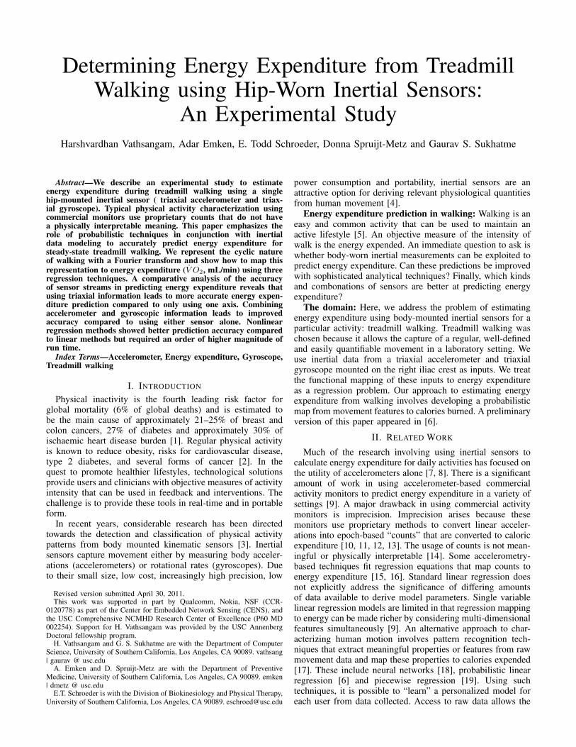
odicity was captured with inertial sensor data from the rightiliac crest. Movement signals corresponded directly to theaccelerations and rotational rates of the hip as measured bythe sensor in its local frame of reference. Fig. 1a showssample inertial data from treadmill walking collected over10 seconds when a participant is walking at a speed of 2.5mph. Regular periodic patterns were observed in steady-state.Similar patterns were observed for other speeds.

B. Variation of Periodicity with SpeedThe periodicity of walking signals was examined by com-

puting their Fourier transforms. Figure 1b illustrates Fouriertransforms of two 10 second steady state walking samplesat 2.5 mph and 3.5 mph for the X-axis acceleration streams.The Fourier transform showed clear peaks indicating distinctperiodic components for the original signals. The peaks oc-curred at the same frequencies for all other sensor streams.The location of these peaks was a function of walking speed.The dominant peak for walking at 3.5 mph occurs at ahigher frequency than the corresponding peak for walkingat 2.5 mph. In prior work, the relationship between energyexpenditure and walking speed has been modeled as one wherewalking at higher speeds requires higher energy expenditure[25, 26, 27]. The fact that each speed exhibits a characteristicfrequency spectrum and that there exists a map between speedand energy expenditure suggests that one can track caloriesexpended in treadmill walking using the frequency spectrumas a representative feature space.

IV. MAPPING WALKING DATA TO ENERGY EXPENDITURE

A. Problem FormulationGiven the representation of treadmill walking using features

described in Sec. III, we focused on the problem of deriving amapping from these features to energy consumed as measuredby V O2 consumption (mL/min). We frame this as a regressionproblem. Consider a D-dimensional input variable x ∈ RD ofwhich there are specific data points {xn}Nn=1. The goal of

regression is to predict the value of one or more continuoustarget variables t of which there are corresponding observedvalues {tn}Nn=1 that are related to the input variables by a“best-fit” function f(xn). This section examines three can-didate algorithms to find this map. We provide descriptionsof each algorithm for the case of an arbitrary D-dimensionalinput variable and one dimensional target variable and discussthe relative merits and demerits of each.

B. Least Squares Linear Regression

Least Squares Regression (LSR) [28] models regression asa linear combination of input variables. Specifically, for aninput data point xn, we have

tn = w0 + w1φ1(xn) + . . . wM−1φM−1(xn) + ε

with ε ∼ N(0, β−1I

)=⇒ tn = wTφ(xn) + ε, ε ∼ N

(0, β−1I

)(1)

where ε is a noise parameter, φ = (φ0, . . . φM−1)T is the

derived function space consisting of fixed nonlinear func-tions of the input variables of dimension M − 1 and w =(w0, . . . , wM−1)

T are the weights . This model is linear in φ.This allows the usage of feature functions {φj(xn)} derivedfrom input variables xn. Equation 1 describes a mapping fromfeature space {φj(xn)} to the output values tn. Given that εis a Gaussian, allowing a probabilistic interpretation, we have:

p(tn|xn,w, β) = N(tn;w

Tφ(xn), β−1) (2)

We define an optimal fitting function as one that maximizes the

likelihood p(t|wTX) =

N∏n=1

p(tn|xn,w, β). This is equivalent

to finding the optimal w that would minimize the expectedsquare-loss ED

{(tn − f(xn,w))

2}

. The optimal predictionis given by:

w =(ΦTΦ

)−1ΦT t

and Φ =

φ0(x1) . . . φM−1(x1)φ0(x2) . . . φM−1(x2)

.... . .

...φ0(xN ) . . . φM−1(xN )

(3)

The optimal prediction for a new data point x∗ is given by:t∗ = wTφ(x∗) (4)

LSR provides a closed-form solution to the regression prob-lem. However it does not explicitly address the significance ofdiffering amounts of data available to derive model parameters.A larger sized dataset with more training examples and stablenoise parameters potentially provides more useful informationfor training a more accurate model than a smaller dataset. LSRis also prone to the presence of outliers because it does not takeinto account the consistency of points in a dataset. Anotherdrawback of LSR is its tendency to over-fit to a given datasetdue to which it often performs poorly on unseen data points.One solution is to include a regularization term λ that controlsthe relative importance of data-dependent noise. Howeverfinding the optimal λ involves techniques such as K-foldcross-validation and the need to maintain a separate validationdataset. These methods can be computationally expensive andwasteful of valuable data. A more elegant solution involves aBayesian treatment of linear regression. Such a technique hasthe potential to guard against over-fitting.

(a) An example of periodic signals obtained from the iliac crest of the right hipwhile walking at a constant speed of 2.5 mph. Steady state walk is cyclic innature and this periodicity can be captured with inertial sensors.

(b) Definite peaks in the Fourier transforms of the accelerometer streamon the X-axis for steady state walking at 2.5 mph and 3.5 mph suggestenergy estimation by monitoring the frequency spectrum.

Figure 1: Representation of periodicity of human walk as captured by inertial sensors

C. Bayesian Linear Regression

Bayesian Linear Regression (BLR) [29] adopts a Bayesianapproach to the linear regression problem by introducing aprior probability distribution over the model parameters w inEquation. 1. Specifically we choose a Gaussian prior over w,p(w) = N

(w;0, α−1I

)where α is a hyperparameter.

Given Equation 2, the prior distribution over w, and theproperties of Gaussians, we can estimate the posterior distri-bution of w given the dataset D as:

p(w|t) = N (mN ,SN )

with mN = βSNΦT t

and S−1N = αI + βΦTΦ

The optimal prediction for a new data point is given by thepredictive distribution by marginalizing over w as:

p(tnew|x∗, t, α, β) = N (mTNφ(x), σ

2N (x∗)) (5)

and σ2N (x∗) =

1

β+ φ(xnew)

TSNφ(x∗) (6)

In a fully Bayesian approach, we adopt hyperpriors over α andβ also and make predictions by marginalizing over w, α and β.However, complete marginalization over all these variables inanalytically intractable. We instead adopt an iterative approachby finding the best α and β to maximize the evidence functiongiven this dataset, find the best parameters w to maximize thelikelihood given a fixed α and β and repeat until convergence.

The output prediction of BLR (Equations 5 and 6) involvescomputing a mean mN and a variance σ2

N (x). The importanceof a variance estimate is that it allows the user to evaluatehow “confident” the algorithm is of its prediction and providesthe necessary tool to evaluate the goodness of prediction ofan unseen data point. Also, it can be seen from Equation 6that if an additional point xN+1 were added, the resultantvariance σ2

N+1(x) < σ2N (x). This tends to the limit σ2

N (x)N→∞

=

1

βor the intrinsic noise in the process. Thus BLR reflects

the availability of larger quantities of data through a smallervariance and hence an increasingly more confident estimate.The use of a prior α helps guard against over-fitting. α and βare derived purely from the dataset without needing a separatevalidation dataset.

Parametric models suffer from a shortcoming in that the

form of the basis functions {φj(x)} are fixed before thetraining data set is observed. If the assumption behind thechoice of basis functions or the linearity of the model is vio-lated, the model will provide poor predictions. An alternativeis to use nonparametric models where the model structureand complexity are not specified in advance but are insteaddetermined from data.

D. Gaussian Process Regression

Given a set of training points{(x1, t1), (x2, t2), . . . , (xn, tn)} such that:

tn = f(xn) + ε, ε ∼ N(0, β−1I

)(7)

a Gaussian Process Regression model (GPR) [30] esti-mates a posterior probability distribution over functionsf (x1), f (x2), . . . f (xN ) evaluated at points x1, x2, . . . xN suchthat any finite subset of the functions is a joint multivari-ate Gaussian distribution. Consequently, for a given set ofpoints x = (x1, x2, . . . xN )T , we have a corresponding vectorFx = (f(x1), f(x2), . . . f(xN ))T that belongs to a multivari-ate Gaussian distribution:

FxN∼ N{µN (x),KN (x,x′)} (8)

where µ(x) is the mean function µ(x) =(µ(x1), µ(x2), . . . µ(xN ))T and K is the covariance orkernel function. The key idea in GPR is that the covariancebetween two function values, f(xi) and f(xj), dependson the input values, xi and xj and is specified via thekernel k(xi,xj). The kernel function returns the covariancebetween the corresponding Fx variables f (xi) and f (xj). Tocompletely specify a GP, it is enough to specify µ(x) andK(x,x′). By definition, each f(xi) is marginally Gaussian,with mean µ(xi) and variance k(xi,xi).

Typically, for ease of implementation, the mean of thedataset is subtracted from each data point so that the meanfunction is 0. To reflect that similar feature vectors with smallinterpoint Euclidean distance are more likely to correspond tothe same output energy consumption measure, and to capturethe inherent common structure represented by feature vectorsdue to an underlying periodicity in walking, we choose theradial basis function kernel. Further, to capture the fact that weonly have access to noisy observations of the function values,it is necessary to add the corresponding covariance function

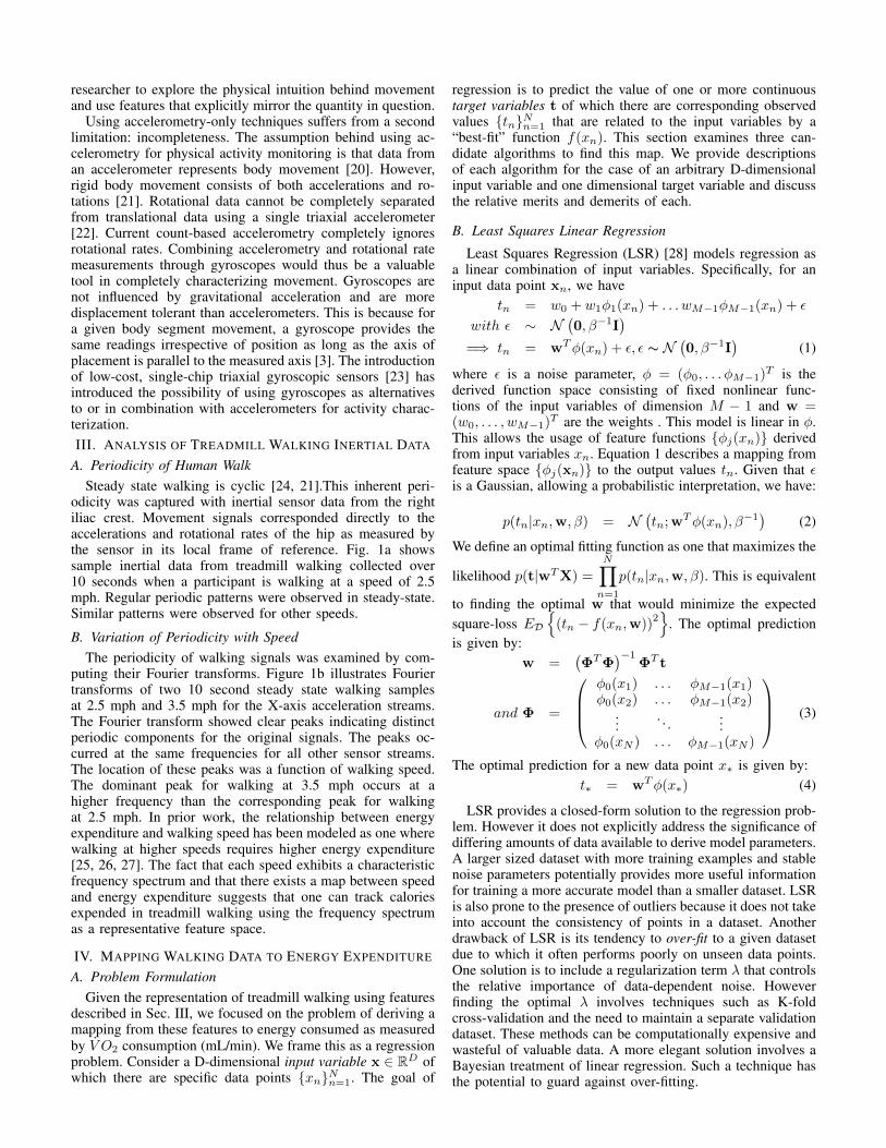
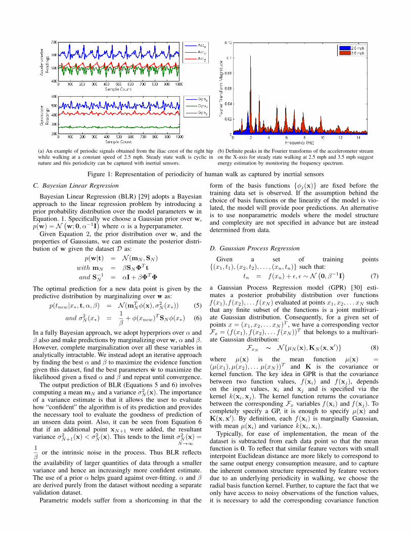
(a) Sensor board used to collect data. (b) The controller board with RN-41 Bluetooth module(c) An example mount of sensor onthe right iliac crest.

Figure 2: Illustration of hardware used to capture treadmill walking information. Acceleration information was collected with aFreescale MMA7260Q triple-axis accelerometer. Rotational rates were collected with 2 Invensense IDG500 500◦/s gyroscopesmounted perpendicular to each other. The sensor hardware was modified to be worn with a custom designed harness on theright iliac crest. Original image source for (a) and (b): www.sparkfun.com

for noisy observations. The complete kernel function can beexpressed in element by element fashion as:

k(xi, xj) = σ2f .e−

1

2l2|xi−xj |2

+ σ2nδij (9)

where σ2f is the signal variance, l is a length scale that

determines strength of correlation between points, σ2n is the

noise variance.For a new point x∗ there exists a corresponding target

quantity f(x∗). Since f(x∗) also belongs to the same GP, itcan be appended to the original training set to obtain a largerset.

FxN+1∼ N{µN (x),KN+1(x,x

′)} (10)

KN+1 =

(KN k∗kT∗ k

)(11)

where k∗ has elements k(xn, x∗) for n = 1, . . . , N andk(xi, xj) is defined in Equation 9. Using properties of Gaus-sians and the definition of GPs, it follows that for a new testpoint p(t∗|x∗,X, t) = N (f (x∗);m(x∗), σ

2x∗). Because this

joint distribution is Gaussian by definition, we have:m(x∗) = kT

∗K−1N t (12)σ2(x∗) = k − kT

∗K−1N k∗ (13)

Thus estimating a target energy from training data amounts toevaluating KN , k and c and using values shown in Equations.12 and 13.

Equations. 12 and 13 summarize the key advantages ofGPR. Again, the use of a probabilistic model to obtaina mean and variance for each prediction allows the userto assess the confidence of each prediction. In contrast toBLR however, GPR is non-parametric: its model complexityincreases with larger quantities of data as evident from theincreasing size of the kernel matrix. GPR avoids the processof explicitly constructing a suitable feature function space bydealing instead with kernel functions. As the kernel implicitlycontains a non-linear transformation, no assumptions aboutthe functional form of the feature space are necessary. This

allows us to deal with non-linear maps without having toconstruct non-linear function spaces. The motivation behindconsidering this algorithm was to determine whether usinga nonlinear probabilistic map (GPR) offers benefits over alinear probabilistic map (BLR) in terms of increased predictionaccuracy.

V. METHODS

A. Hardware DescriptionHuman movement was captured with a modified version

of the Sparkfun 6DoF Inertial Measurement Unit (IMU) v4[31]. Fig. 2 illustrates the hardware used. The v4 providesthree axes of acceleration data, three axes of gyroscopicdata, and three axes of magnetic data with three sensors: aFreescale MMA7260Q triple-axis accelerometer, set at 1.5 gsensitivity and two InvenSense IDG500 500◦/s gyroscopes.At the time of this study, the absence of triaxial gyroscopesrequired that two biaxial gyroscopes be mounted perpendicularto each other and calibrated to function as one gyroscope.Control was through an LPC2138 ARM7 processor. Customfirmware was used on the controller board to stream sensordata continuously. Data were sampled at 100 Hz. The unitused Bluetooth to transmit data to either a nearby PC ormobile phone using the RN41 Bluetooth module set at 115200bps. Maximum range of the transmitter was approximately5 m in indoor conditions. The system was powered from a3.3V rechargeable lithium-polymer battery power supply. Thesensor was encased in a custom-designed harness to be wornon the right iliac crest (participants were asked to wear theharness tightly to prevent any slippage). The use of sensors inall three axes allowed the capture of periodicity in all threeplanes – sagittal, frontal and transverse. The treadmill used forthe experiments was the research quality NordicTrack A2550PRO. Fig. 7a illustrates the recording procedure [6].

B. Participant StatisticsSeven healthy adults (three male, four female) participated

in the study. Height and weight of each participant wererecorded using a Healthometer balance beam scale. The par-ticipants had average age = 29 ± 6 years, average height =

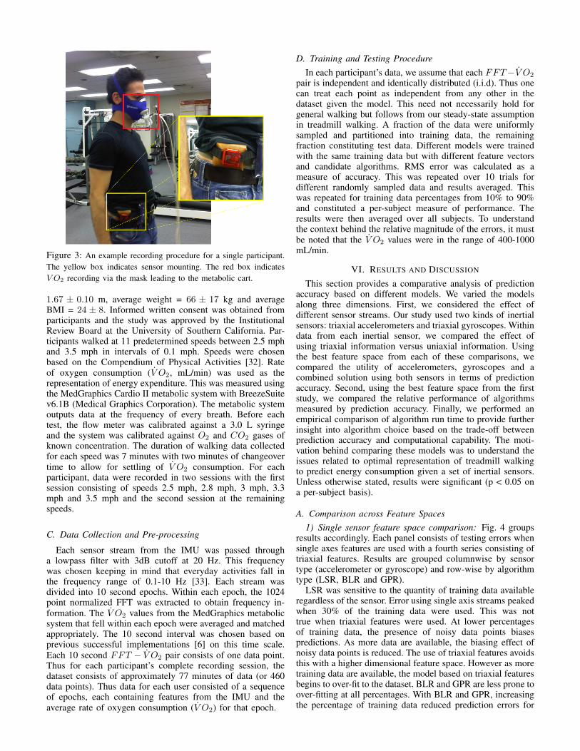
Figure 3: An example recording procedure for a single participant.The yellow box indicates sensor mounting. The red box indicatesV O2 recording via the mask leading to the metabolic cart.

1.67 ± 0.10 m, average weight = 66 ± 17 kg and averageBMI = 24 ± 8. Informed written consent was obtained fromparticipants and the study was approved by the InstitutionalReview Board at the University of Southern California. Par-ticipants walked at 11 predetermined speeds between 2.5 mphand 3.5 mph in intervals of 0.1 mph. Speeds were chosenbased on the Compendium of Physical Activities [32]. Rateof oxygen consumption (V O2, mL/min) was used as therepresentation of energy expenditure. This was measured usingthe MedGraphics Cardio II metabolic system with BreezeSuitev6.1B (Medical Graphics Corporation). The metabolic systemoutputs data at the frequency of every breath. Before eachtest, the flow meter was calibrated against a 3.0 L syringeand the system was calibrated against O2 and CO2 gases ofknown concentration. The duration of walking data collectedfor each speed was 7 minutes with two minutes of changeovertime to allow for settling of V O2 consumption. For eachparticipant, data were recorded in two sessions with the firstsession consisting of speeds 2.5 mph, 2.8 mph, 3 mph, 3.3mph and 3.5 mph and the second session at the remainingspeeds.

C. Data Collection and Pre-processing

Each sensor stream from the IMU was passed througha lowpass filter with 3dB cutoff at 20 Hz. This frequencywas chosen keeping in mind that everyday activities fall inthe frequency range of 0.1-10 Hz [33]. Each stream wasdivided into 10 second epochs. Within each epoch, the 1024point normalized FFT was extracted to obtain frequency in-formation. The V O2 values from the MedGraphics metabolicsystem that fell within each epoch were averaged and matchedappropriately. The 10 second interval was chosen based onprevious successful implementations [6] on this time scale.Each 10 second FFT − V O2 pair consists of one data point.Thus for each participant’s complete recording session, thedataset consists of approximately 77 minutes of data (or 460data points). Thus data for each user consisted of a sequenceof epochs, each containing features from the IMU and theaverage rate of oxygen consumption (V O2) for that epoch.

D. Training and Testing ProcedureIn each participant’s data, we assume that each FFT−V O2

pair is independent and identically distributed (i.i.d). Thus onecan treat each point as independent from any other in thedataset given the model. This need not necessarily hold forgeneral walking but follows from our steady-state assumptionin treadmill walking. A fraction of the data were uniformlysampled and partitioned into training data, the remainingfraction constituting test data. Different models were trainedwith the same training data but with different feature vectorsand candidate algorithms. RMS error was calculated as ameasure of accuracy. This was repeated over 10 trials fordifferent randomly sampled data and results averaged. Thiswas repeated for training data percentages from 10% to 90%and constituted a per-subject measure of performance. Theresults were then averaged over all subjects. To understandthe context behind the relative magnitude of the errors, it mustbe noted that the V O2 values were in the range of 400-1000mL/min.

VI. RESULTS AND DISCUSSION

This section provides a comparative analysis of predictionaccuracy based on different models. We varied the modelsalong three dimensions. First, we considered the effect ofdifferent sensor streams. Our study used two kinds of inertialsensors: triaxial accelerometers and triaxial gyroscopes. Withindata from each inertial sensor, we compared the effect ofusing triaxial information versus uniaxial information. Usingthe best feature space from each of these comparisons, wecompared the utility of accelerometers, gyroscopes and acombined solution using both sensors in terms of predictionaccuracy. Second, using the best feature space from the firststudy, we compared the relative performance of algorithmsmeasured by prediction accuracy. Finally, we performed anempirical comparison of algorithm run time to provide furtherinsight into algorithm choice based on the trade-off betweenprediction accuracy and computational capability. The moti-vation behind comparing these models was to understand theissues related to optimal representation of treadmill walkingto predict energy consumption given a set of inertial sensors.Unless otherwise stated, results were significant (p < 0.05 ona per-subject basis).

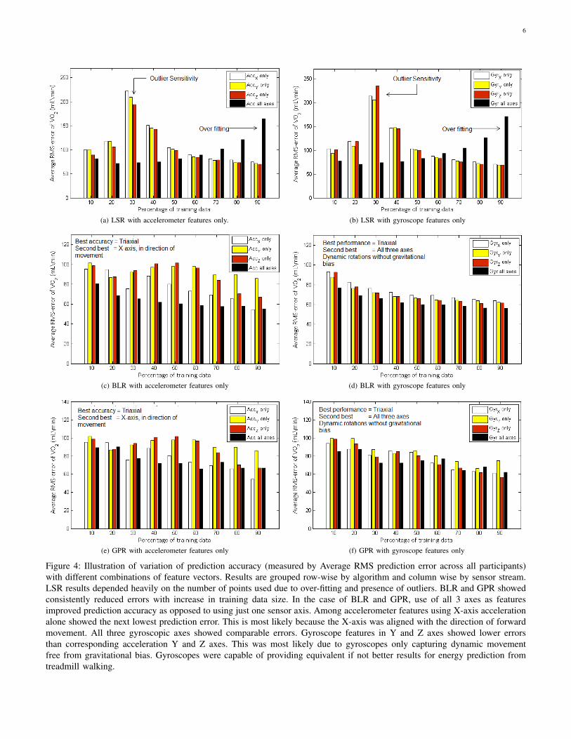
A. Comparison across Feature Spaces1) Single sensor feature space comparison: Fig. 4 groups

results accordingly. Each panel consists of testing errors whensingle axes features are used with a fourth series consisting oftriaxial features. Results are grouped columnwise by sensortype (accelerometer or gyroscope) and row-wise by algorithmtype (LSR, BLR and GPR).

LSR was sensitive to the quantity of training data availableregardless of the sensor. Error using single axis streams peakedwhen 30% of the training data were used. This was nottrue when triaxial features were used. At lower percentagesof training data, the presence of noisy data points biasespredictions. As more data are available, the biasing effect ofnoisy data points is reduced. The use of triaxial features avoidsthis with a higher dimensional feature space. However as moretraining data are available, the model based on triaxial featuresbegins to over-fit to the dataset. BLR and GPR are less prone toover-fitting at all percentages. With BLR and GPR, increasingthe percentage of training data reduced prediction errors for

6

(a) LSR with accelerometer features only. (b) LSR with gyroscope features only

(c) BLR with accelerometer features only (d) BLR with gyroscope features only

(e) GPR with accelerometer features only (f) GPR with gyroscope features only

Figure 4: Illustration of variation of prediction accuracy (measured by Average RMS prediction error across all participants)with different combinations of feature vectors. Results are grouped row-wise by algorithm and column wise by sensor stream.LSR results depended heavily on the number of points used due to over-fitting and presence of outliers. BLR and GPR showedconsistently reduced errors with increase in training data size. In the case of BLR and GPR, use of all 3 axes as featuresimproved prediction accuracy as opposed to using just one sensor axis. Among accelerometer features using X-axis accelerationalone showed the next lowest prediction error. This is most likely because the X-axis was aligned with the direction of forwardmovement. All three gyroscopic axes showed comparable errors. Gyroscope features in Y and Z axes showed lower errorsthan corresponding acceleration Y and Z axes. This was most likely due to gyroscopes only capturing dynamic movementfree from gravitational bias. Gyroscopes were capable of providing equivalent if not better results for energy prediction fromtreadmill walking.

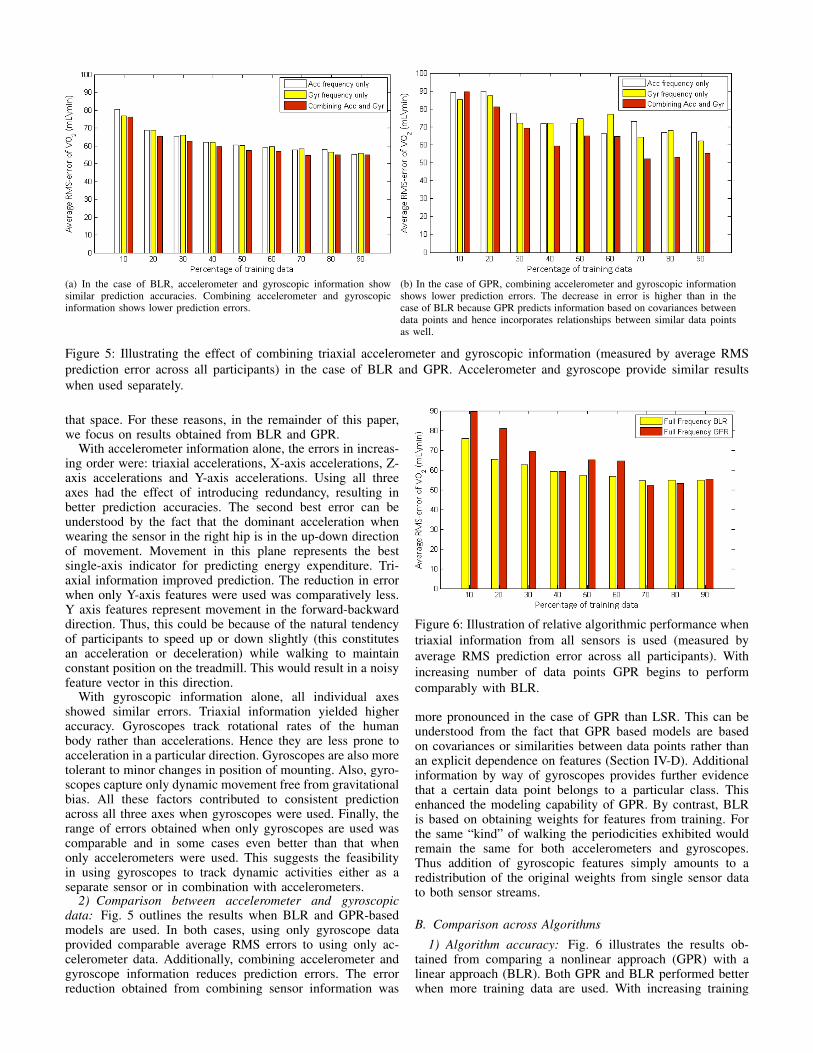
(a) In the case of BLR, accelerometer and gyroscopic information showsimilar prediction accuracies. Combining accelerometer and gyroscopicinformation shows lower prediction errors.

(b) In the case of GPR, combining accelerometer and gyroscopic informationshows lower prediction errors. The decrease in error is higher than in thecase of BLR because GPR predicts information based on covariances betweendata points and hence incorporates relationships between similar data pointsas well.

Figure 5: Illustrating the effect of combining triaxial accelerometer and gyroscopic information (measured by average RMSprediction error across all participants) in the case of BLR and GPR. Accelerometer and gyroscope provide similar resultswhen used separately.

that space. For these reasons, in the remainder of this paper,we focus on results obtained from BLR and GPR.

With accelerometer information alone, the errors in increas-ing order were: triaxial accelerations, X-axis accelerations, Z-axis accelerations and Y-axis accelerations. Using all threeaxes had the effect of introducing redundancy, resulting inbetter prediction accuracies. The second best error can beunderstood by the fact that the dominant acceleration whenwearing the sensor in the right hip is in the up-down directionof movement. Movement in this plane represents the bestsingle-axis indicator for predicting energy expenditure. Tri-axial information improved prediction. The reduction in errorwhen only Y-axis features were used was comparatively less.Y axis features represent movement in the forward-backwarddirection. Thus, this could be because of the natural tendencyof participants to speed up or down slightly (this constitutesan acceleration or deceleration) while walking to maintainconstant position on the treadmill. This would result in a noisyfeature vector in this direction.

With gyroscopic information alone, all individual axesshowed similar errors. Triaxial information yielded higheraccuracy. Gyroscopes track rotational rates of the humanbody rather than accelerations. Hence they are less prone toacceleration in a particular direction. Gyroscopes are also moretolerant to minor changes in position of mounting. Also, gyro-scopes capture only dynamic movement free from gravitationalbias. All these factors contributed to consistent predictionacross all three axes when gyroscopes were used. Finally, therange of errors obtained when only gyroscopes are used wascomparable and in some cases even better than that whenonly accelerometers were used. This suggests the feasibilityin using gyroscopes to track dynamic activities either as aseparate sensor or in combination with accelerometers.

2) Comparison between accelerometer and gyroscopicdata: Fig. 5 outlines the results when BLR and GPR-basedmodels are used. In both cases, using only gyroscope dataprovided comparable average RMS errors to using only ac-celerometer data. Additionally, combining accelerometer andgyroscope information reduces prediction errors. The errorreduction obtained from combining sensor information was

Figure 6: Illustration of relative algorithmic performance whentriaxial information from all sensors is used (measured byaverage RMS prediction error across all participants). Withincreasing number of data points GPR begins to performcomparably with BLR.

more pronounced in the case of GPR than LSR. This can beunderstood from the fact that GPR based models are basedon covariances or similarities between data points rather thanan explicit dependence on features (Section IV-D). Additionalinformation by way of gyroscopes provides further evidencethat a certain data point belongs to a particular class. Thisenhanced the modeling capability of GPR. By contrast, BLRis based on obtaining weights for features from training. Forthe same “kind” of walking the periodicities exhibited wouldremain the same for both accelerometers and gyroscopes.Thus addition of gyroscopic features simply amounts to aredistribution of the original weights from single sensor datato both sensor streams.

B. Comparison across Algorithms

1) Algorithm accuracy: Fig. 6 illustrates the results ob-tained from comparing a nonlinear approach (GPR) with alinear approach (BLR). Both GPR and BLR performed betterwhen more training data are used. With increasing training

data, GPR performance improved gradually until it was com-parable with BLR. Nonlinear approaches require more data tobe able to capture nonlinear subtleties and prevent over-fittingto noise. When data from each subject were considered, GPRshowed a lower average RMS prediction error when comparedwith BLR and LSR when a larger relative percentage oftraining data was used. This indicates that GPR shows superiorperformance when a large quantity of data are available. Withsmaller quantities of data it would be advisable to use BLRto prevent over-fitting.

Fig. 7a illustrates an example output for energy predictionfor a single participant using the feature space and algorithmcombination that provides the lowest prediction error. Themodel uses triaxial features from both accelerometer andgyroscope axes and GPR with 80% of the data used fortraining. The predicted values (shown in blue) closely matchthe ground truth (shown in red). Fig. 7b shows the same dataas a scatter plot with ground truth displayed on the X-axisand GPR predicted values on the Y-axis. The two times seriesshowed an average correlation of 0.92 across users.

C. Algorithm Run TimeParametric approaches like linear regression depend on the

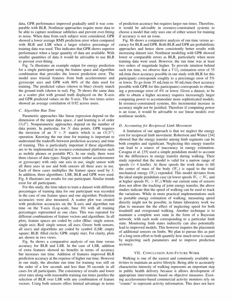
dimension of the input data space, d and learning is of orderO(d3). Nonparametric approaches depend on the number ofdata points. In particular, for N data points, GPR requiresthe inversion of an N × N matrix which is an O(N3)operation. Knowing the run time for training is important tounderstand the tradeoffs between prediction accuracy and timeof training. This is particularly important if these algorithmsare to be implemented in resource-constrained platforms suchas mobile phones or portable PCs. In our study, there werethree classes of data types: Single sensor (either accelerometeror gyroscope) with only one axis in use, single sensor withall three axes in use and both sensors all three axes in use.Each of these cases multiplies the feature space used by 3.In addition, three algorithms: LSR, BLR and GPR were used.Fig. 8 illustrates our results for one participant. Similar trendsexist for all participants.

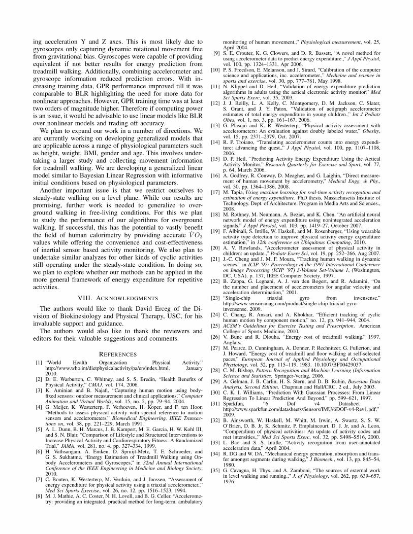
For this study, the time taken to train a dataset with differentpercentages of training data for one participant was recordedin the case of one feature space and one algorithm. Predictionaccuracies were also measured. A scatter plot was createdwith prediction accuracies on the X-axis and algorithm runtime on the Y-axis (Log-scale, base 10) with all trainingpercentages represented as one class. This was repeated fordifferent combinations of feature vectors and algorithms. In allplots, feature spaces are coded by color (Blue: single sensor,single axis; Red: single sensor, all axes; Green: both sensors,all axes) and algorithms are coded by symbol (LSR: emptysquare; BLR: filled circle; GPR: empty star). For clarity, plotsare shown in two views.

Fig. 8a shows a comparative analysis of run time versusaccuracy for BLR and LSR. In the case of LSR, additionof extra features showed no benefits in terms of accuracybut increases run time. Addition of features improved BLRprediction accuracy at the expense of higher run time. Howeverin our study, the absolute run time for training was still onthe order of a few seconds and less than 30 seconds in allcases for all participants. The consistency of results and lowererror rates along with reasonable training run times justifies theselection of BLR over LSR with any combination of featurevectors. Using both sensors offers limited advantage in terms

of prediction accuracy but requires larger run times. Therefore,it would be advisable in resource-constrained systems tochoose a model that only uses one of either sensor for trainingif accuracy is not an issue.

Fig. 8b shows a comparative analysis of run time versus ac-curacy for BLR and GPR. Both BLR and GPR are probabilisticapproaches and hence show consistently better results withincreasing dataset size. Nonlinear modeling with GPR showedlower or comparable errors as BLR, particularly when moretraining data were used. However, the run time was at leasttwo orders of magnitude higher. To provide intuition behindsuch run time, we observe that a V O2 estimation error of 35mL/min (best accuracy possible in our study with BLR for thisparticipant) corresponds roughly to a percentage error of 5%or lower. To go from 35 mL/min to 30 mL/min (best accuracypossible with GPR for this participants) corresponds to obtain-ing a percentage error of 4% or lower. Given a dataset, to beable to obtain a higher accuracy requires increasingly largercomputing power to accommodate more sophisticated models.In resource-constrained systems, this incremental increase inaccuracy might not be justified. Therefore if computing poweris an issue, it would be advisable to use linear models overnonlinear models.

D. Accounting for Reciprocal Limb MovementA limitation of our approach is that we neglect the energy

cost for reciprocal limb movement. Robertson and Winter [34]showed that the energy transfer among limb segments can beboth complex and significant. Neglecting this energy transfercan lead to a source of inaccuracy in energy estimation.Cavagna et al. [35] used a simple pendulum model to accountfor the differences in energy transfer during walking. Theirstudy reported that the model is valid for a narrow range ofspeeds (≈ 4 km/hr). At these speeds the work done to liftthe center of mass of the body (Wv) is equal to the totalmechanical energy (Wt) expended. This model deviates fromthe ideal simple pendulum case (at lower speeds Wt < Wv andat higher speeds Wt > Wv).While our current suite of sensorsdoes not allow the tracking of joint energy transfer, the abovestudies indicate that the speed of walking can be used to trackthe variations. While in more practical implementations suchas portable energy estimation of walking, measuring speeddirectly might not be possible, in future laboratory work weplan to measure the the effect of neglecting speed for bothtreadmill and overground walking. Another technique is tomaintain a complete user state in the form of a Bayesiannetwork, with each node corresponding to a particular limbstate. Monitoring limb states indirectly can also potentiallylead to improved models. This however requires the placementof additional sensors on limbs. We plan to pursue this as partof a long term effort to both quantify how much error is causedby neglecting such parameters and to improve predictionaccuracy.

VII. CONCLUSION AND FUTURE WORK

Walking is one of the easiest and commonly available ac-tivities to maintain an active lifestyle. Being able to accuratelycharacterize intensity of walking represents an important stepin public health delivery because it allows development ofappropriate interventions based on objective measures. Exist-ing accelerometer-based commercial activity monitors rely on“counts” to represent activity information. This does not have

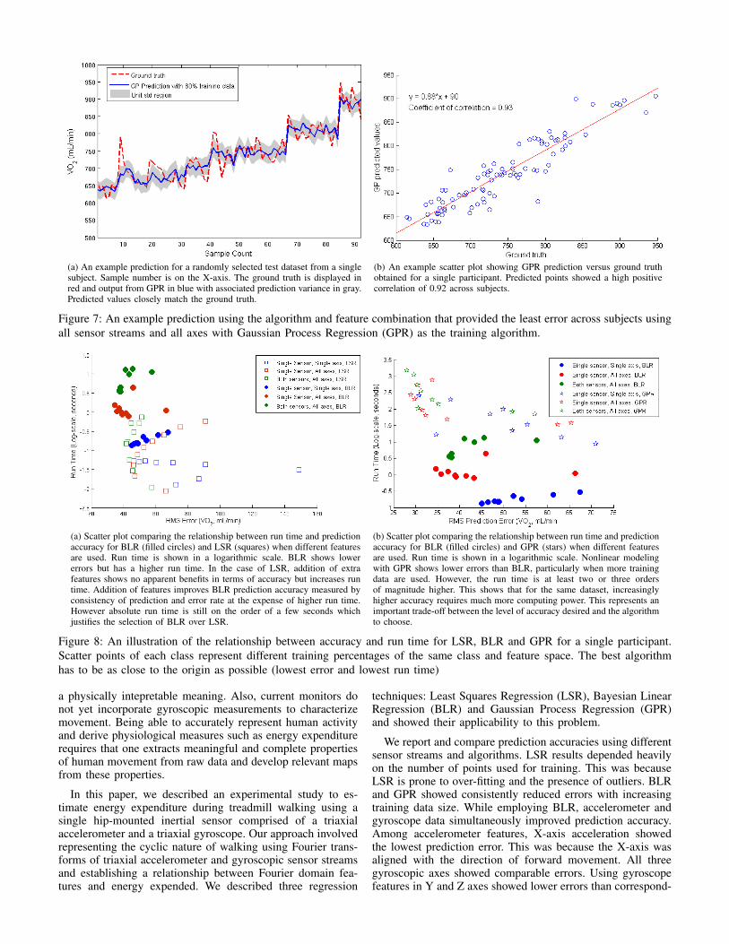
(a) An example prediction for a randomly selected test dataset from a singlesubject. Sample number is on the X-axis. The ground truth is displayed inred and output from GPR in blue with associated prediction variance in gray.Predicted values closely match the ground truth.

(b) An example scatter plot showing GPR prediction versus ground truthobtained for a single participant. Predicted points showed a high positivecorrelation of 0.92 across subjects.

Figure 7: An example prediction using the algorithm and feature combination that provided the least error across subjects usingall sensor streams and all axes with Gaussian Process Regression (GPR) as the training algorithm.

(a) Scatter plot comparing the relationship between run time and predictionaccuracy for BLR (filled circles) and LSR (squares) when different featuresare used. Run time is shown in a logarithmic scale. BLR shows lowererrors but has a higher run time. In the case of LSR, addition of extrafeatures shows no apparent benefits in terms of accuracy but increases runtime. Addition of features improves BLR prediction accuracy measured byconsistency of prediction and error rate at the expense of higher run time.However absolute run time is still on the order of a few seconds whichjustifies the selection of BLR over LSR.

(b) Scatter plot comparing the relationship between run time and predictionaccuracy for BLR (filled circles) and GPR (stars) when different featuresare used. Run time is shown in a logarithmic scale. Nonlinear modelingwith GPR shows lower errors than BLR, particularly when more trainingdata are used. However, the run time is at least two or three ordersof magnitude higher. This shows that for the same dataset, increasinglyhigher accuracy requires much more computing power. This represents animportant trade-off between the level of accuracy desired and the algorithmto choose.

Figure 8: An illustration of the relationship between accuracy and run time for LSR, BLR and GPR for a single participant.Scatter points of each class represent different training percentages of the same class and feature space. The best algorithmhas to be as close to the origin as possible (lowest error and lowest run time)

a physically intepretable meaning. Also, current monitors donot yet incorporate gyroscopic measurements to characterizemovement. Being able to accurately represent human activityand derive physiological measures such as energy expenditurerequires that one extracts meaningful and complete propertiesof human movement from raw data and develop relevant mapsfrom these properties.

In this paper, we described an experimental study to es-timate energy expenditure during treadmill walking using asingle hip-mounted inertial sensor comprised of a triaxialaccelerometer and a triaxial gyroscope. Our approach involvedrepresenting the cyclic nature of walking using Fourier trans-forms of triaxial accelerometer and gyroscopic sensor streamsand establishing a relationship between Fourier domain fea-tures and energy expended. We described three regression

techniques: Least Squares Regression (LSR), Bayesian LinearRegression (BLR) and Gaussian Process Regression (GPR)and showed their applicability to this problem.

We report and compare prediction accuracies using differentsensor streams and algorithms. LSR results depended heavilyon the number of points used for training. This was becauseLSR is prone to over-fitting and the presence of outliers. BLRand GPR showed consistently reduced errors with increasingtraining data size. While employing BLR, accelerometer andgyroscope data simultaneously improved prediction accuracy.Among accelerometer features, X-axis acceleration showedthe lowest prediction error. This was because the X-axis wasaligned with the direction of forward movement. All threegyroscopic axes showed comparable errors. Using gyroscopefeatures in Y and Z axes showed lower errors than correspond-

ing acceleration Y and Z axes. This is most likely due togyroscopes only capturing dynamic rotational movement freefrom gravitational bias. Gyroscopes were capable of providingequivalent if not better results for energy prediction fromtreadmill walking. Additionally, combining accelerometer andgyroscope information reduced prediction errors. With in-creasing training data, GPR performance improved till it wascomparable to BLR highlighting the need for more data fornonlinear approaches. However, GPR training time was at leasttwo orders of magnitude higher. Therefore if computing poweris an issue, it would be advisable to use linear models like BLRover nonlinear models and trading off accuracy.

We plan to expand our work in a number of directions. Weare currently working on developing generalized models thatare applicable across a range of physiological parameters suchas height, weight, BMI, gender and age. This involves under-taking a larger study and collecting movement informationfor treadmill walking. We are developing a generalized linearmodel similar to Bayesian Linear Regression with informativeinitial conditions based on physiological parameters.

Another important issue is that we restrict ourselves tosteady-state walking on a level plane. While our results arepromising, further work is needed to generalize to over-ground walking in free-living conditions. For this we planto study the performance of our algorithms for overgroundwalking. If successful, this has the potential to vastly benefitthe field of human calorimetry by providing accurate V O2

values while offering the convenience and cost-effectivenessof inertial sensor based activity monitoring. We also plan toundertake similar analyzes for other kinds of cyclic activitiesstill operating under the steady-state condition. In doing so,we plan to explore whether our methods can be applied in themore general framework of energy expenditure for repetitiveactivities.

VIII. ACKNOWLEDGMENTS

The authors would like to thank David Erceg of the Di-vision of Biokinesiology and Physical Therapy, USC, for hisinvaluable support and guidance.

The authors would also like to thank the reviewers andeditors for their valuable suggestions and comments.

REFERENCES[1] “World Health Organization - Physical Activity.”

http://www.who.int/dietphysicalactivity/pa/en/index.html, January2010.

[2] D. E. Warburton, C. Whitney, and S. S. Bredin, “Health Benefits ofPhysical Activity,” CMAJ, vol. 174, 2006.

[3] K. Aminian and B. Najafi, “Capturing human motion using body-fixed sensors: outdoor measurement and clinical applications,” ComputerAnimation and Virtual Worlds, vol. 15, no. 2, pp. 79–94, 2004.

[4] G. Meijer, K. Westerterp, F. Verhoeven, H. Koper, and F. ten Hoor,“Methods to assess physical activity with special reference to motionsensors and accelerometers,” Biomedical Engineering, IEEE Transac-tions on, vol. 38, pp. 221–229, March 1991.

[5] A. L. Dunn, B. H. Marcus, J. B. Kampert, M. E. Garcia, H. W. Kohl III,and S. N. Blair, “Comparison of Lifestyle and Structured Interventions toIncrease Physical Activity and Cardiorespiratory Fitness: A RandomizedTrial,” JAMA, vol. 281, no. 4, pp. 327–334, 1999.

[6] H. Vathsangam, A. Emken, D. Spruijt-Metz, T. E. Schroeder, andG. S. Sukhatme, “Energy Estimation of Treadmill Walking using On-body Accelerometers and Gyroscopes,” in 32nd Annual InternationalConference of the IEEE Engineering in Medicine and Biology Society,2010.

[7] C. Bouten, K. Westerterp, M. Verduin, and J. Janssen, “Assessment ofenergy expenditure for physical activity using a triaxial accelerometer.,”Med Sci Sports Exercise, vol. 26, no. 12, pp. 1516–1523, 1994.

[8] M. J. Mathie, A. C. Coster, N. H. Lovell, and B. G. Celler, “Accelerome-try: providing an integrated, practical method for long-term, ambulatory

monitoring of human movement.,” Physiological measurement, vol. 25,April 2004.

[9] S. E. Crouter, K. G. Clowers, and D. R. Bassett, “A novel method forusing accelerometer data to predict energy expenditure.,” J Appl Physiol,vol. 100, pp. 1324–1331, Apr 2006.

[10] P. S. Freedson, E. Melanson, and J. Sirard, “Calibration of the computerscience and applications, inc. accelerometer.,” Medicine and science insports and exercise, vol. 30, pp. 777–781, May 1998.

[11] N. Klippel and D. Heil, “Validation of energy expenditure predictionalgorithms in adults using the actical electronic activity monitor,” MedSci Sports Exerc, vol. 35, 2003.

[12] J. J. Reilly, L. A. Kelly, C. Montgomery, D. M. Jackson, C. Slater,S. Grant, and J. Y. Paton, “Validation of actigraph accelerometerestimates of total energy expenditure in young children.,” Int J PediatrObes, vol. 1, no. 3, pp. 161–167, 2006.

[13] G. Plasqui and K. R. Westerterp, “Physical activity assessment withaccelerometers: An evaluation against doubly labeled water,” Obesity,vol. 15, pp. 2371–2379, Oct. 2007.

[14] R. P. Troiano, “Translating accelerometer counts into energy expendi-ture: advancing the quest.,” J Appl Physiol, vol. 100, pp. 1107–1108,2006.

[15] D. P. Heil, “Predicting Activity Energy Expenditure Using the ActicalActivity Monitor,” Research Quarterly for Exercise and Sport, vol. 77,p. 64, March 2006.

[16] A. Godfrey, R. Conway, D. Meagher, and G. Laighin, “Direct measure-ment of human movement by accelerometry,” Medical Engg. & Phy.,vol. 30, pp. 1364–1386, 2008.

[17] M. Tapia, Using machine learning for real-time activity recognition andestimation of energy expenditure. PhD thesis, Massachusetts Institute ofTechnology. Dept. of Architecture. Program in Media Arts and Sciences.,2008.

[18] M. Rothney, M. Neumann, A. Beziat, and K. Chen, “An artificial neuralnetwork model of energy expenditure using nonintegrated accelerationsignals,” J Appl Physiol, vol. 103, pp. 1419–27, October 2007.

[19] F. Albinali, S. Intille, W. Haskell, and M. Rosenberger, “Using wearableactivity type detection to improve physical activity energy expenditureestimation,” in 12th conference on Ubiquitous Computing, 2010.

[20] A. V. Rowlands, “Accelerometer assessment of physical activity inchildren: an update.,” Pediatr Exerc Sci, vol. 19, pp. 252–266, Aug 2007.

[21] J.-C. Cheng and J. M. F. Moura, “Tracking human walking in dynamicscenes,” in ICIP ’97: Proceedings of the 1997 International Conferenceon Image Processing (ICIP ’97) 3-Volume Set-Volume 1, (Washington,DC, USA), p. 137, IEEE Computer Society, 1997.

[22] B. Zappa, G. Legnani, A. J. van den Bogert, and R. Adamini, “Onthe number and placement of accelerometers for angular velocity andacceleration determination,” 2001.

[23] “Single-chip triaxial gyro from invensense.”http://www.sensorsmag.com/product/single-chip-triaxial-gyro-invensense, 2009.

[24] C. Chang, R. Ansari, and A. Khokhar, “Efficient tracking of cyclichuman motion by component motion,” no. 12, pp. 941–944, 2004.

[25] ACSM’s Guidelines for Exercise Testing and Prescription. AmericanCollege of Sports Medicine, 2010.

[26] V. Bunc and R. Dlouha, “Energy cost of treadmill walking,” 1997.Anglais.

[27] M. Pearce, D. Cunningham, A. Donner, P. Rechnitzer, G. Fullerton, andJ. Howard, “Energy cost of treadmill and floor walking at self-selectedpaces,” European Journal of Applied Physiology and OccupationalPhysiology, vol. 52, pp. 115–119, 1983. 10.1007/BF00429037.

[28] C. M. Bishop, Pattern Recognition and Machine Learning (InformationScience and Statistics. Springer-Verlag, 2006.

[29] A. Gelman, J. B. Carlin, H. S. Stern, and D. B. Rubin, Bayesian DataAnalysis, Second Edition. Chapman and Hall/CRC, 2 ed., July 2003.

[30] C. K. I. Williams, “Prediction With Gaussian Processes: From LinearRegression To Linear Prediction And Beyond,” pp. 599–621, 1997.

[31] Sparkfun, “6 Dof v4 Datasheet -http://www.sparkfun.com/datasheets/Sensors/IMU/6DOF-v4-Rev1.pdf,”2009.

[32] B. Ainsworth, W. Haskell, M. Whitt, M. Irwin, A. Swartz, S. S. W.O’Brien, D. B. Jr, K. Schmitz, P. Emplaincourt, D. J. Jr, and A. Leon,“Compendium of physical activities: An update of activity codes andmet intensities.,” Med Sci Sports Exerc, vol. 32, pp. S498–S516, 2000.

[33] L. Bao and S. S. Intille, “Activity recognition from user-annotatedacceleration data,” April 2004.

[34] R. DG and W. DA, “Mechanical energy generation, absorption and trans-fer amongst segments during walking,” J Biomech., vol. 13, pp. 845–54,1980.

[35] G. Cavagna, H. Thys, and A. Zamboni, “The sources of external workin level walking and running.,” J. of Physiology, vol. 262, pp. 639–657,1976.

11

Harshvardhan Vathsangam received the B. Tech.degree in Engineering Physics from the Indian Insti-tute of Technology Madras, Chennai, India in 2008.He is currently a PhD student with the RoboticEmbedded Systems Laboratory, Viterbi School ofEngineering, University of Southern California, LosAngeles, CA. He is a recipient of the AnnenbergGraduate Fellowship. His research interests are inthe application of statistical machine learning tech-niques for inertial data from the human body forphysical activity detection and energy expenditure

monitoring.

B. Adar Emken received the B.S. in BehavioralNeuroscience from Ohio State University, Dublin,OH in 2001 and the Ph.D. in Neurosience fromUniversity of California, Irvine in 2008.She joined the Department of Health Promotion andDisease Prevention, University of Southern Califor-nia, Los Angeles, CA, in 2008 as a Postdoctoralfellow, to design a wireless body area network(WBAN) to detect and intervene on physical activityin real-time for overweight youth.

E. Todd Schroeder received the B.S. in HumanPhysiology from the University of California atDavis in 1992, the Ph.D. in Biokinesiology from theUniversity of Southern California (Clinical ExercisePhysiology), Los Angeles, CA in 2000.He is currently an Assistant Professor of ClinicalPhysical Therapy at the Division of Biokinesiol-ogy and Physical Therapy, University of SouthernCalifornia, Los Angeles, CA. His primary researchinterest is in the mechanisms whereby progressiveresistance training and testosterone treatment stimu-

late protein synthesis and improve muscle quality in older persons. Additionalresearch interests include understanding the mechanisms (signals/factors)associated with eccentric resistance exercise that induces hypertrophic adap-tations and the implications of such exercise in older individuals to optimizerehabilitation.

Donna Spruijt-Metz received the B.S. degree inPsychology from the University of Amsterdam, TheNetherlands in 1986, the M.S. degree in Psychology(Research Methods) from the University of Am-sterdam, The Netherlands in 1991 and the Ph.D.in Adolescent Health/Medical Ethics from the FreeUniversity, Amsterdam, The Netherlands in 1996.She is currently an Associate Professor of Researchat the Department of Preventive Medicine, KeckSchool of Medicine. Her research focuses on pe-diatric obesity, human motivation and adolescent

health, particularly in the areas of diet and physical activity. Current researchincludes a longitudinal study of the impact of puberty on insulin dynamics,mood and physical activity in African American and Latina girls, and an in-labfeeding study to determine the acute effects of high sugar meals on physicalactivity and other metabolic outcomes in African American and Latino youth.

Gaurav S. Sukhatme received the B. Tech. degreein Computer Science and Engineering from theIndian Institute of Technology Bombay, Mumbai,India and the M.S. and Ph.D. degrees in ComputerScience from USC.He is a Professor of Computer Science (joint ap-pointment in Electrical Engineering) at the Univer-sity of Southern California (USC). He is the co-director of the USC Robotics Research Laboratoryand the director of the USC Robotic EmbeddedSystems Laboratory which he founded in 2000. He

is a fellow of the IEEE and a recipient of the NSF CAREER award and theOkawa foundation research award. He is the Editor-in-Chief of AutonomousRobots and has served as Associate Editor of the IEEE Transactions onRobotics and Automation, the IEEE Transactions on Mobile Computing, andon the editorial board of IEEE Pervasive Computing.