determination of convective heat … of convective heat-transfer coefficients on adiabatic walls...

DETERMINATION OF CONVECTIVE HEAT-TRANSFER COEFFICIENTS ON ADIABATIC WALLS USING A SINUSOIDALLY FORCED FLUID TEMPERATURE

~

~ by Ronald G. Huff _. --

Lewis Research Center Cleveland, Ohio

1.1. lr .n ,_ .-.- .... .-..a ..... -.-- ...- -.....- . . . . . a . . . - - m . - C . C . . . . . I . CI . I . In .ZC. . I m c N A I I U N A L A t K U N A U I I L 3 ANU 3 r A L t A U M I N I 3 I K A I I U N WAJnlNUIUN, U. L. JUIYL I T 0 0

https://ntrs.nasa.gov/search.jsp?R=19680015146 2018-06-09T23:12:06+00:00Z

NASA TM X-1594

DETERMINATION OF CONVECTIVE HEAT-TRANSFER

COEFFICIENTS ON ADIABATIC WALLS USING A

SINUSOIDALLY FORCED FLUID TEMPERATURE

By Ronald G. Huff

Lewis Research Center Cleveland, Ohio

For sale by the Clearinghouse for Federal Scientific and Technical Information Springfield, Virginia 22151 - CFSTI price $3.00

ABSTRACT

The response of an insulated wall, over which a heated fluid flows, to a sinusoidally forced fluid temperature was used to calculate the convective heat-transfer coefficients. An exact solution i s given which accounts for thermal conductivity and the location of the sensed wall temperature in one-dimensional heat-transfer problems. Charts a r e in- cluded to a id in the calculation. A comparative analysis was made of solutions that do not account for thermal conductivity and the location of the sensed wall temperature and those that do. If the exact solution i s not used, e r r o r s greater than 23 percent a r e possible.

STAR Category 33

ii

DETERMINATION OF CONVECTIVE HEAT-TRANSFER COEFFICIENTS

ON ADIABATIC WALLS USING A SINUSOIDALLY FORCED

FLU I D TEMPERATURE

by Ronald G. Huff

Lewis Research Center

SUMMARY

The response of an insulated wall, over which a heated fluid flows, to a sinusoidally forced fluid temperature was used to calculate the convective heat-transfer coefficients. An exact solution is given which accounts for thermal conductivity and the location of the sensed wall temperature in one-dimensional heat-transfer problems. Charts are in- cluded to aid in the calculation. A comparative analysis was made of solutions that do not account for thermal conductivity and the location of the sensed wall temperature and those that do. If the exact solution is not used, e r r o r s greater than 23 percent are possible.

INTRODUCTION

Both t ransient and steady-state analyses have been used to design calor imeters for u s e in rocket engines and aerodynamic heat-transfer studies. The steady-state calorim- eter makes use of the temperature gradient in a material of known conductivity and geom- etry; the t ransient type makes use of the response of a mater ia l to a driving temperature, that is, the response of a thin disk to a step change in the surrounding fluid.

The response of a wall to a fluid that flows over it and has a sinusoidally oscillating temperature has been used to calculate the convective heat-transfer coefficient h. The solution found by Anderson (ref. 1) for the convective heat-transfer coefficient (herein called slug solution), however, does not account for thermal conductivity o r the location of the measured wall temperature. An estimate, given by Anderson, of "the e r r o r in the measured t ime constant T caused by heat conduction through the skin" is 1 . 5 percent. Bell (ref. 2) neglects the effect of thermal conductivity by designing h i s experiments in zzdi 8 -vvzy iis ti, cause its eiiect to drop out of his equations, which are in s e r i e s form.

The objective of this analytical investigation, conducted at NASA Lewis Research Center, was to find a solution fo r the convective heat-transfer coefficient as a function of the phase l a g between the fluid and wall temperatures. Such a solution would take into account the thermoconductivity as well as the location of the measured wall temperature.

The solution is presented along with charts that (for the wall temperature measured a t the insulated side of the wall) can be used to determine the heat-transfer coefficient as a function of frequency, wall properties, wall thickness, and phase lag. A comparison is made between this solution and that of Anderson (ref. l), both of which assume that the back surface of the wall x = L is perfectly insulated.

The slug solution may be substituted for the present analysis when conductivity and temperature-sensor location are not important.

SYMBOLS

C specific heat of wall material , Btu/(lb) (OR) ; J/(kg) (K)

CON

f

h

K

L

T

T -

ATG X

CY

€G

e 17

71

function defined in eq. (4b)

frequency of temperature oscillation, cps; Hz

convective heat-transfer coefficient on surface of wall, Btu/(in. ?(sec)('R) ; W/(m2) (K)

thermal conductivity, Btu/(in. ) (sec) (OR) ; J/(m) (sec) (K)

thickness of wall, in. ; m

wall temperature, Tw - TG,

mean temperature, OR; K

- 0

R; K

- 0 amplitude of gas temperature, TG - TG,

distance measured from fluid-wall interface into wall, in. ; m

thermal diffusivity, K/pC

function defined after eq. (49

frequency and diffusivity per imeter , a i time. s ec

R; K

constant equal to 3.1416 rad density of wall material , lb/in. 3; kg/m 3

time constant, pCL/h

P

7

2

cp phase shift between forced fluid temperature TG and wall temperature Tw, < 0 for Tw lagging TG, deg

o angular velocity of forced fluid temperature T 2nf rad/sec

Subs c r ip t s :

G fluid flowing over wall

s

w

G'

values calculated with Anderson's slug-type solution (ref. 1)

wall over which fluid flows

DIFFERENTIAL EQUATIONS AND ASSUMPTIONS

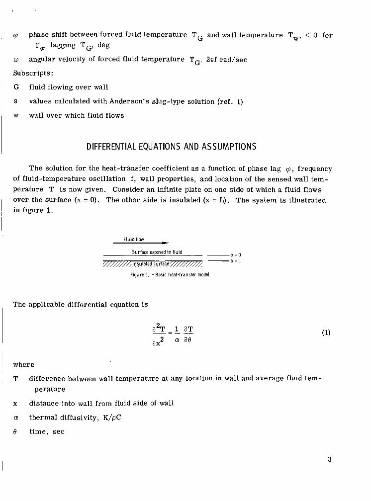
The solution for the heat-transfer coefficient a s a function of phase lag q , frequency of fluid-temperature oscillation f , wall properties, and location of the sensed wall temperature T is now given. Consider an infinite plate on one side of which a fluid flows over the surface (x = 0). The other side is insulated (x = L) . The system is illustrated in figure 1.

f l u i d flow -

x - 0 x - L

Surface exposed to f lu id

///////// ,Insulated surface =///////// L Figure 1. - Basic heat-transfer model.

The applicable differential equation is

a2T - 1 aT - - - - 2 CY ae ax

where

T difference between wall temperature at any location in wall and average fluid tempera ture

x

a! thermal diffusivity, K/pC

8 t ime, s ec

distance into wall f rom fluid side of wall

3

This solution assumes that the (1) Thermal conductivity is finite and constant (2) Convective heat-transfer coefficient h is constant (3) Density p and specific heat C of the wall are constant (4) Surface of the wal l at x = L is insulated (5) Surface of the wall at x = 0 is exposed to a fluid whose temperature is given by

where

fluid temperature

average fluid temperature TG

TG -

ATG amplitude of gas temperature

w angular velocity of temperature oscillation, 2nf rad/sec

(6) Convective heat t ransfer at x = 0 is

aT ax G G - T ) -K- = h (T (3)

(7) Heat conduction through the wall is one dimensional

For the solution to the differential equation (l), a product solution is assumed and the boundary conditions are applied (i. e . , an insulated surface at x = L, assumption (4), and convective heat t ransfer at x = 0, assumption (6). The details of the solution are given in the appendix. The convective heat-transfer coefficient is

where

for the wall temperature lagging the fluid tempera ture

4

e 27?(L-x) cos q(2L - x) + cos 77x

e 2q(L-x) sin q ( 2 ~ - x) + sin qx A b , L, =

where

q 2 a

This solution is simplified if the wall temperature is measured at x = L, which for - many applications is the easiest place to locate a sensor. The CON used in equation (4a) reduces to

- CON = tan(q - qL) at x = L ( 4 4

The solutions to equation (1) may be used to determine the convective heat-transfer coefficient when thermal conductivity is an important factor.

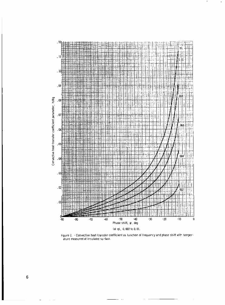
The computations made for the convective heat-transfer coefficient with the present solution (eqs. (4)) are t ime consuming. The values for h/Kq were calculated as a function of qL and q , when x = L, and are plotted in figure 2 . Using x = L (temperature sensor located at the insulated surface) is reasonable because a temperature sensor is easily installed at this point.

The ratio of the amplitude of the wall- to the fluid-temperature oscillation for x = L can be written by inspection of equation (A15). The ratio is

L

T G - T G ATG 1/ - e271LE sin(EG+ 2qL) 1’ 1 - 9 + e2qLE cos(eG + 2qL) - hG

where

5

F

L Y .

-90 -80 -70 -60 -50 -40 -30 -20 -10 0 Phase shift, (p, deg

(a) qL. 0.002 to 0.01.

Figure 2. - Convective heat-transfer coefficient as function of frequency and phase shif t with ternper- ature measured at insulated surface.

6

Phase shift, (0, deg

(bl 7L. 0.008toO.1.

Figure 2. - Continued.

7

1

1

1

F Y 8

c C

V ._ .- E I 0)

VI C L

E c c 0) 8

-200 -180 -160 -140 -120 -100 -80 -60 -40 -20 0 Phase shift, (p, deq

(c) VL. 0. 1 to 3.0.

Figure 2. -Concluded.

8

l

and

-1 1 c G = tan - -t 1 K?7

hG

This ratio can be used to determine the magnitude of the fluid-temperature oscillation T G that would yield a measurable wall-temperature oscillation at x = L.

The determination of the effect of wall properties and plate thickness L on the calculation of h was aided by the expanding of equation (4a) to a s e r i e s form at x = L. The resulting equation for hG is

- -- 2 5 t a n q -tan q 3 tan q

In this equation, 40 < 0. Convergence of this se r ies must be checked. However, if qL << 1 and reasonable values of q (e. g. , -450, a r e used, the s e r i e s wil l converge.

equates the r a t e of change of the temperature of a mass o r slug pL to the convective In this repor t , Anderson's solution is referred to as the slug solution because it

heat t ransfer f rom a differential equation

fluid that flows over the slug. The slug solution is derived from the

- TG 7- - - tTW- aTW

ae

and assumes that (1) The thermal conductivity K is infinite (i .e. , no temperature gradient in the

(2) The convective heat-transfer coefficient h is constant (3) The density p and specific heat C of the wall a r e constant (4) One wall surface is insulated (5) The other wall surface is exposed to a fluid whose temperature is given by

wall)

- TG = TG + ATG sin we

The solution to the differential equation (5) is

9

where

is the time constant. The phase lag between the wall and the fluid is tan-' WT = cp S from which the convective heat-transfer coefficient can be written as

-pCLw tan cps

hG, s =

where cps is < 0.

CRITERION FOR USE OF SLUG SOLUTION

Comparison of the series form of the present solution (eq. (4g)) for hG with that of the s lug solution (eq. (8)) shows that the coefficient of the series solution is simply hG, s .

If hG, second power are neglected, the series solution can be written as

i s substituted in the series solution and all t e r m s having powers greater than

2

3 tan cp (qL)2 . . . hG 3 + t a n cp - = I - -

hG, s

where <p < 0, and q L is assumed to be much smaller than 1. The value of cp can and should be approximately -45' (as discussed in the section Optimum Phase Angle). The curves in figure 2 can be used to determine the proper frequency that, fo r a given material, qL, and hG, will yield the value cp = -45'. The selected value of qL is then used in equation (sa) along with cp = -45' to evaluate the ratio hJhG, s . F o r these

conditions, equation (sa) reduces to

4 2 = 1 + - 2 L -hG, , -- hG - - l + - ( q L ) . . . 3 3 K hG, s

10

v ) - w m ~ m m c u t - C r . . . . . N

0- 0 3 -

I L

0 , I I I . I I I I

L - l o l l

A m 4 - d 0 0 0 0 0 0 0 0 0 0 0 . . . . .

w m m 4 * N N W A N w 3 0 0 . . . . . 3 * N N W

3 N * ' r ( O 0 . . . . .

3

0 3

OD i $ w w e a * 3 - m - m O O N O D v )

A A A . . . . .

O O O N O w * - m ( D 0 0 0 0 0 0 . . . . .

W N m

0 t-

m N 3

0

m In N 0 0 0

0

N m m 3

0 0 0 3

11

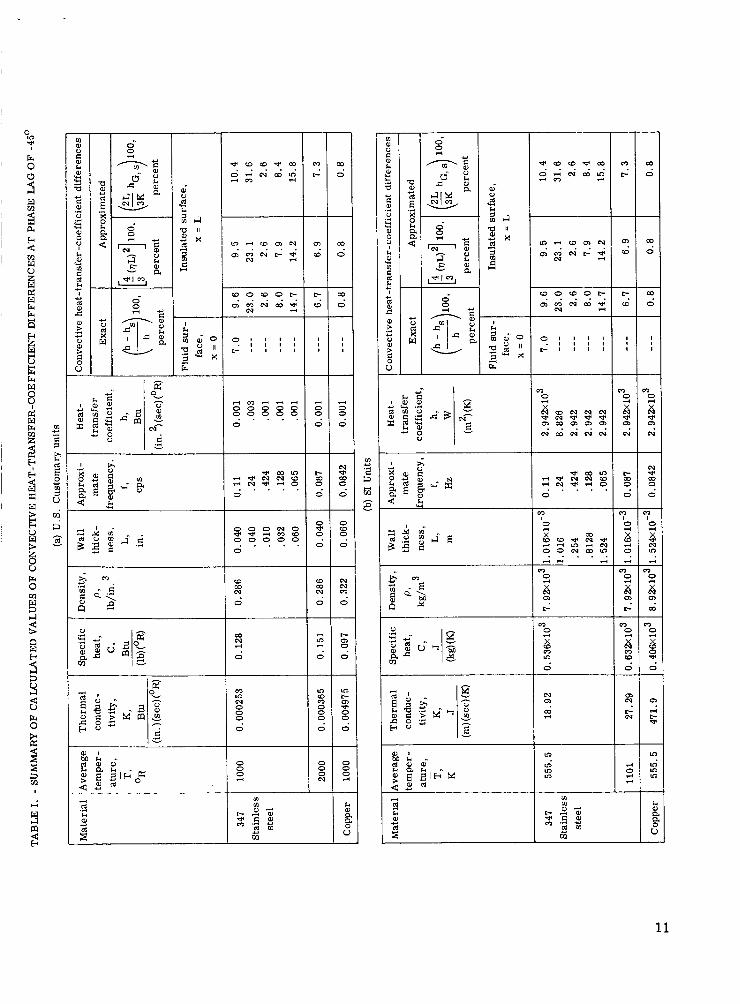
where <p = -45' and qL << 1. The second term in equation (9b), a n approximation to (h - hs)/h, can be used to approximate the e r r o r in h if the slug solution, instead of the present solution, is used to calculate h. The term may also be used as a f i rs t -order correction if the slug solution is used to calculate h.

Values for the second te rm in equation (9b) were calculated for 347 stainless steel and copper and are compared in table I with the values of (h - hs)/h X 100 percent. The agreement is good, even though the absolute value of the difference is large in several cases. Care must be exercised in using equations (sa) and (9b) because only two t e r m s of the series are used, and if the value of qL approaches 1, convergence is not ensured. In addition, Values f o r <p that approach either 0' o r 90' will greatly affect hJhG, s .

In addition to the aforementioned cr i te r ia to be used in the choice of solutions fo r calculating h, a number of calculations were made and are presented to illustrate the practical application of the solutions f i r s t given for h .

APPLICATION OF EQUATIONS TO ENGINEERING MATERIALS

The calculation of the relation between phase lag angle <p and forcing frequency f necessitates that assumptions be made for values of the convective heat-transfer coefficient and the properties of the wall. The value of the convective heat-transfer coefficient hG assumed in this calculation is 0.001 Btu p e r square inch per second pe r '€3 (2. 942X103 W/(m2)(K)), unless otherwise noted. The wall properties used are those of 347 stainless steel and are given as follows:

Average temperature, T, OR; K . . . . . . . . . . . . . . . . . . . . . . . . 1000; 555.5

3 Specific heat, C, Btu/(lb)('R); J/(kg)(K) . . . . . . . . . . . . . . . . . 0.128; 0.536X10 Conductivity, K, Btu/(in. ) (sec) (OR) ; J/(m) (sec) (K) . . . . . . . . . . . 0.000253; 18.92

These values are approximately those of 347 skiinless -steel mater ia ls used for simulated rocket-nozzle heat-transfer studies conducted in an air facility. The value of hG is approximately 5 to 10 t imes greater than those found by Anderson (ref. 1) in his wind-tunnel t e s t s on a cone.

Density, p , lb/in.3; kg/m 3 . . . . . . . . . . . . . . . . . . . . . . . . 0.286; 7.92X103

Comparison of Phase Lags

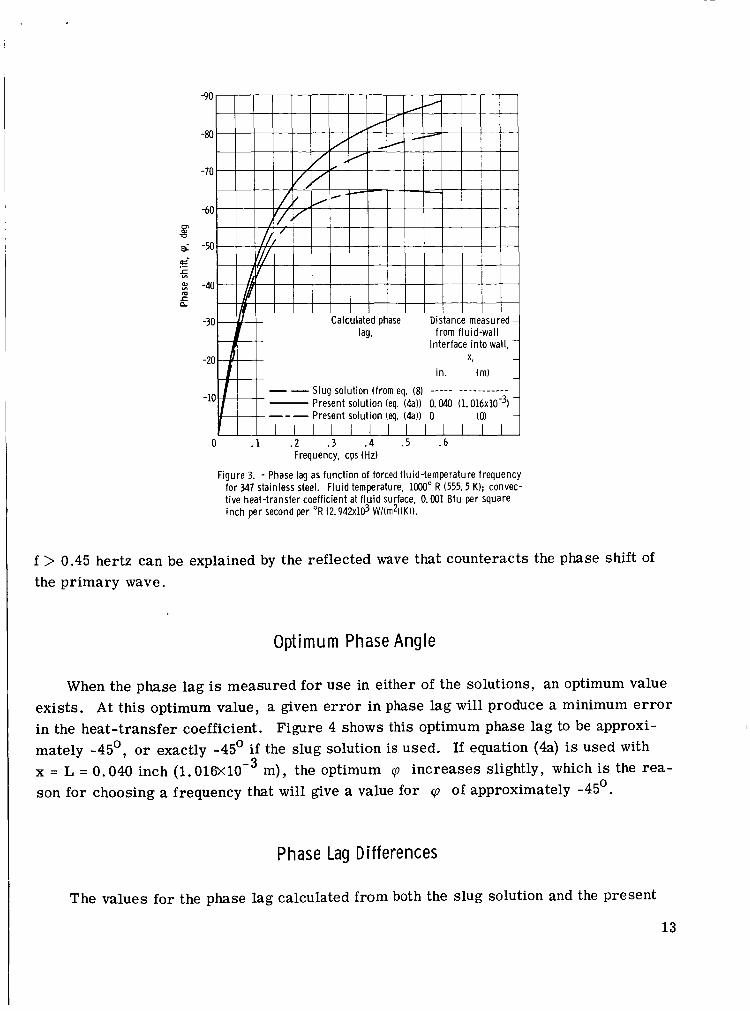
The calculated phase lags 40 as a function of frequency f are shown in figure 3. AS would be expected, the slug solution phase l a g falls between the values calculated with equation (4a) (present solution) a t x = 0 and at x = L . The decrease in cp a t x = 0 f o r

12

in. (m)

Slug solution (from eq. (8) ----- ----------- Present solution (eq. (4a)) 0.040 ( 1 . 0 1 6 ~ 1 0 ~ ) Present solution (eq. (4a)) 0 ( 0)

-loH-- ---

0 . 1 . 2 .3 . 4 . 5 .6 Frequency, cps (Hz)

Figure 3. - Phase lag as function of forced fluid-temperature frequency for 347 stainless steel. Fluid temperature, 1 0 " R (555.5 K); convective heat-transfer coefficient at f lu id surface, 0.001 Btu per square i nch per second per O R (2 .942~10~ W/(m*NK)).

f > 0.45 hertz can be explained by the reflected wave that counteracts the phase shift of the pr imary wave.

Optimum Phase Angle

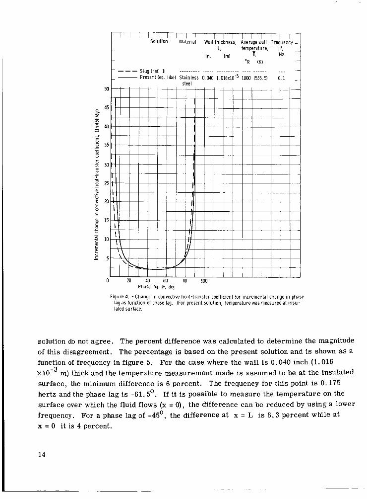
When the phase lag is measured for use in either of the solutions, an optimum value exists. A t this optimum value, a given e r r o r in phase lag will produce a minimum e r r o r in the heat-transfer coefficient. Figure 4 shows this optimum phase lag to be approximately -45O, or exactly -45' if the slug solution is used. If equation (4a) is used with x = L = 0.040 inch ( l . O l 6 ~ l O - ~ m), the optimum q increases slightly, which is the rea- son for choosing a frequency that will give a value fo r q of approximately -45'.

Phase Lag Differences

The values f o r the phase lag calculated from both the slug solution and the present

13

- Solution Material Wall

-

- "R (K)

-

in. (m)

Slug (ref. 1) _ _ _ _ _ _ _ _ _ _ _ _ _ _ _ _ _ _ _ _ _ _ _ _ _ _ _ _ _ _ _ _ _ _ --- - Present (eq. ( 4 4 Stainless 0.040 1 . 0 1 6 ~ 1 0 - ~ 1000 (555.5)

steel

Phase lag, p, deg

Figure 4. - Change in convective heat-transfer coefficient for incremental change in phase lag as function of phase lag. (For present solution, temperature was measured at i n s u - lated surface.

solution do not agree. The percent difference was calculated to determine the magnitude of this disagreement. The percentage is based on the present solution and is shown as a function of frequency in figure 5.

m) thick and the temperature measurement made is assumed to be at the insulated surface, the minimum difference is 6 percent . The frequency for this point is 0.175 hertz and the phase lag is -61.5'. If it is possible to measure the tempera ture on the surface over which the fluid flows (x = 0), the difference can be reduced by using a lower frequency. For a phase lag of -45', the difference at x = L is 6.3 percent while at x = 0 i t is 4 percent.

For the case where the wall is 0.040 inch (1.016

14

1(

z

e

4

i

0 - c al

al cz 2

-2 E- 5 .....

s" - -4

9 1 Y

-6 I d

2 V tz G)

D -8 -

L L .- c VI

-10 m c a

-12

-14

-16

-18

Frequency, f, cps (Hz)

Figure 5. - Difference in phase lag due to location of temperature sensor as funct ion of frequency for 347 stainless steel. Fluid temperature, 1OOO" R (555.5 K); convective heat-transfer coefficient at f lu id surface, 0.001 Btu per second per "R (2.942~103 W I ness, 0.040 i n c h (1. C16x10-

100

80

60

40 c al u L a n

20 3-

e" 0

5 -20

- .c 2

c c5

c

a, 2

-a -40 L L

c a, U

c

.- .- c - 8 -60 Y

& -80

L aa VI - L c

c m a? c

>

U al >

u

~ -1oc

s -12c

.- c

-14C

-16C

-180 c .1 . 2 . 3 . 4 . 5 . 6 Frequency, f. cps, (Hz)

Figure 6. - Difference in convective heat-transfer CO- efficient due to location of wall temperature sensor as funct ion of frequency for 347 stainless steel. Fluid temperature, 1OOO" R (555.5 K); convective heat- transfer coefficient at f lu id surface, 0.001 Btu r

wall thickness, 0.040 i n c h ( 1 . 0 1 6 ~ 1 0 ~ m). square i n c h per second per "R ( 2 . 9 4 2 ~ 1 0 ~ W/(m T )(K));

15

Heat -T r a n s f e r -C oe f f ic ie n t D i f f e r e nce s

Since a minimum value of the phase lag differences in the case where x = L was ob- served in figure 5, a similar minimum would be expected to exist when the heat-transfer- coefficient differences are calculated. Figure 6, however, shows that the lowest possible difference calculated fo r x = L is greater than 7 percent and occurs at a lower frequency than does the minimum phase lag difference shown in figure 5. At phase lags of -45', the heat-transfer-coefficient differences are 9.6 percent at x = L and 7 percent at x = 0. The differences will increase with increased frequency o r phase lag angle.

Effect of Heat-Transfer Coeff icient

Up to this point in the calculation, the convective heat-transfer coefficient has been

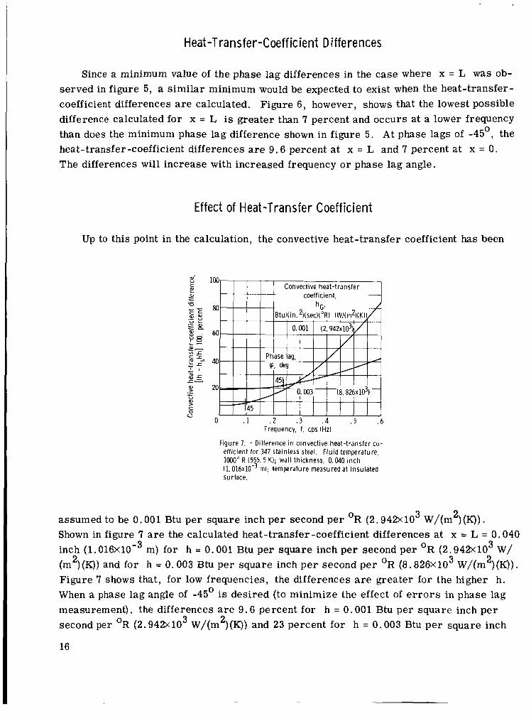
Figure 7. - Difference i n convective heat-transfer coefficient for M7 stainless steel. Fluid temperature, 1oOO" R (555.5 KI; wall thickness. 0.040 inch (1.016~10-~ ml; temperature measured at insulated surface.

3 2 assumed to be 0.001 Btu pe r square inch p e r second p e r OR (2.942X10 W/(m )(K)). Shown in figure 7 are the calculated heat-transfer-coefficient differences at x = L = 0.040

3 inch ( 1 . 0 1 6 ~ 1 0 - ~ m) for h = 0.001 Btu p e r square inch p e r second p e r OR ( 2 . 9 4 2 ~ 1 0 W/ 2 2 (m )(K)) and for h = 0.003 Btu p e r square inch p e r second p e r OR (8. 826X103 W/(m )(K)).

Figure 7 shows that, for low frequencies, the differences are greater for the higher h. When a phase lag angle of -45' is desired (to minimize the effect of e r r o r s in phase lag measurement), the differences are 9 . 6 percent for h = 0.001 Btu per square inch p e r second per OR ( 2 . 9 4 2 ~ 1 0 ~ W/(m )(K)) and 23 percent f o r h = 0.003 Btu p e r square inch

16

2

3 2 per second per OR (8 .826~10 W/(m )(K)). With a phase shift of -45' used as a criterion, it is concluded that increasing the heat-transfer coefficient will increase the heat- transfer-coefficient difference.

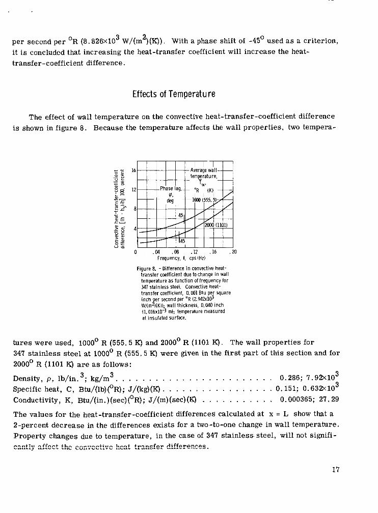
Effects of Temperature

The effect of wall temperature on the convective heat-transfer-coefficient difference is shown in figure 8. Because the temperature affects the wall properties, two tempera-

16

12

8

4

I45

Frequency, f, cps (Hz)

Figure 8. - Difference in convective heat- t ransfer coefficient due to change in wall temperature as funct ion of frequency for 347 stainless steel. Convective heat- transfer coefficient, 0.001 Btu per square inch er second per "R (2.942xld

(1.016~10-3 m); temperature measured at insulated surface.

I

0 .04 .08 .12 .16 .20

W/(m i NK)); wall thickness, 0.040 i nch

lures were used, 1000° R (555.5 K) and 2000' R (1101 K). The wall properties for 347 stainless steel at 1000° R (555.5 K) were given in the first par t of this section and for 2000' R (1101 K) a r e as follows:

Density, p , lb/in. 3; kg/m3. . . . . . . . . . . . . . . . . . . . . . . . 0.286; 7 . 9 2 ~ 1 0 ~ Specific heat, C , Btu/(lb)(%); J/(kg)(K) . . . . . . . . . . . . . . . . . 0.151; 0.63%10 Conductivity, K, Btu/(in. ) (sec) (OR) ; J/(m) (sec) (K) . . . . . . . . . . .

3

0.000365; 27.29

The values for the heat-transfer-coefficient differences calculated a t x = L show that a 2-percent decrease in the differences exists for a two-to-one change in wall temperature. Proper ty changes due to temperature, in the case of 347 stainless steel , will not signifi- cazt!y affect the c ~ ~ v e z t t v z k2,t C,r2&!3.r C'iffPrPnCPC

17

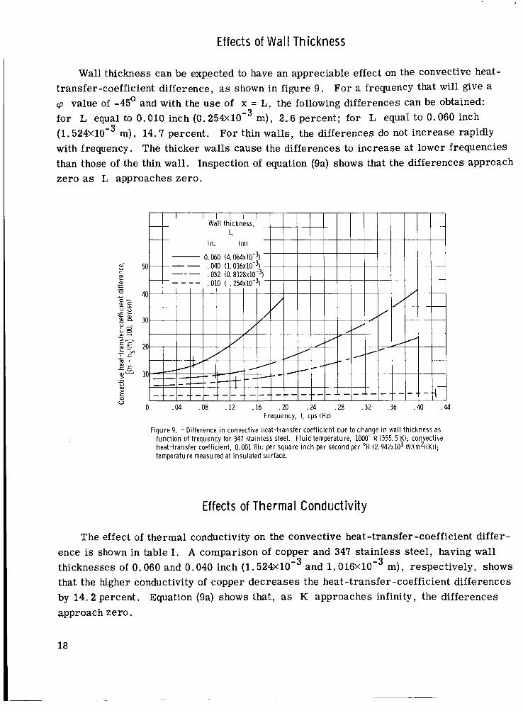
Effects of Wal l Thickness

Effects of Thermal Conduct iv i ty

The effect of thermal conductivity on the convective heat-transfer-coefficient difference is shown in table I. A comparison of copper and 347 stainless s tee l , having wall thicknesses of 0.060 and 0.040 inch ( 1 . 5 2 4 ~ 1 0 - ~ and 1. 0i6X10-3 m) , respectively, shows that the higher conductivity of copper dec reases the heat-transfer-coefficient differences by 14.2 percent. Equation (sa) shows that, as K approaches infinity, the differences approachzero.

i a

~

Wall thickness can be expected to have an appreciable effect on the convective heat- transfer-coefficient difference, as shown in figure 9 . For a frequency that will give a cp value of -45' and with the use of x = L, the following differences can be obtained: for L equal to 0.010 inch ( 0 . 2 5 4 ~ 1 0 - ~ m), 2.6 percent; for L equal to 0.060 inch ( 1 . 5 2 4 ~ 1 0 - ~ m), 14.7 percent. For thin walls, the differences do not increase rapidly with frequency. The thicker walls cause the differences to increase at lower frequencies than those of the thin wall. Inspection of equation (9a) shows that the differences approach ze ro as L approaches zero.

0 .M .08 .12 .16 . M .24 .28 . 3 2 .36 .40 .44 frequency, f, cps (Hz)

Figure 9. - Difference in convective heat-transfer coefficient due to change in wall thickness as function of frequency for 347 stainless steel. Fluid temperature, 1000" R (555. 5 K); convective heat-transfer coefficient, 0.001 Btu per square i nch per second per "R ( 2 . 9 4 2 ~ 1 0 ~ W/(m21(K)I; temperature measured at insulated surface.

COMPARISON OF SOLUTIONS

The slug solution (ref. 1), which neglects the effect of thermal conductivity and temperature-measurement location, may be used in place of the more complicated solution (eqs. (4)) provided that the system is designed properly. Equation (4g) may be used to estimate the e r r o r in h when the slug solution is used provided that qL < 1 .0 . If a maximum e r r o r of 6 percent is to be tolerated, qL cannot exceed 0 . 2 and q must be approximately -45'. Improper design will result in large e r r o r s . Fo r example, a wall made of 347 stainless steel , 0.060 inch ( 1 . 5 2 4 ~ 1 0 - ~ m) thick, with the temperature measured at the insulated face will give e r r o r s greater than 23 percent if phase lags exceed -45'. Inspection of equation (4g) shows that if the slug solution is used, thin walls are essential. Although low frequency improves the accuracy of the slug solution, it is well to keep in mind that, at least for x = L, the limit of hG/hG, # 1. Also, the accuracy in the measurement of the phase lag angle becomes very poor as cp approaches zero (see fig. 4). High thermal conductivity is desirable as are low density and specific heat. If the phase lag is -45O, an increase in the heat-transfer coefficient will increase the e r r o r when the slug solution is used (see fig. 7). An increase in the wall temperature of 347 stainless steel from 1000° to 2000' R (555.5 to 1101 K) resulted in only a %-percent change in the e r r o r (fig. 8).

Table I summarizes the resu l t s of the comparison made of equations (4a) to (4e) and (8). This table presents calculations made for phase lags of -45'.

CONCLUDING REMARKS

The convective heat-transfer coefficient h can be calculated for a fluid flowing over a surface with one insulated side if the fluid temperature is varied sinusoidally. The phase lag between the fluid and wall temperatures, along with the frequency of oscillation and wall mater ia l propert ies , can be used to calculate the convective heat-transfer coefficient h. Two solutions for h are available. Both require a phase lag of approximately -45' to minimize the e r r o r in h due to e r r o r s made in measuring the phase lag angle. Anderson's slug solution (ref. 1) does not account for the wall thermal conductivity o r the location of the measured wall temperature, which may result in an e r r o r greater than 23 percent in h.

19

A general one-dimensional solution is given which accounts for a finite thermal conductivity and fo r the wall-temperature location. This solution is greatly simplified if the wall temperature is measured at the insulated surface. Neither solution is applicable when two- o r three-dimensional heat t ransfer in the wall is important.

Lewis Research Center, National Aeronautics and Space Administration,

Cleveland, Ohio, March 25, 1968, 122-29 -07 -03-22.

20

APPENDIX - DERIVATION OF HEAT-TRANSFER COEFFICIENT

AS FUNCTION OF PHASE LAG

Determination of Boundary Condit ions

The temperature response of a wall , which has one surface insulated at x = L and the other surface exposed to a fluid with a temperature that var ies sinusoidally at x = 0, is calculated a s follows: First, the boundary conditions a r e determined with the assumption that

TG = ATGe -iw8

Fo r x = 0,

For x = L

ax

The governing differential equation is

~

For the solution to the differential equation, assume a product solution

Then

21

and

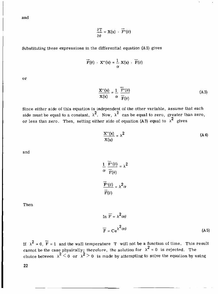
Substituting these expressions in the differential equation (A 1) gives

- 1 - F(8) X"(X) = - X(X) - F(8)

Ly

o r

Since either side of this equation is independent of the other variable, assume that each side must be equal to a constant, A . Now, h can be equal to zero, greater than zero, o r less than zero. Then, setting either side of equation (A3) equal to h2 gives

2 2

and

Then

- x2ae F = Ce

- 2 If A = 0, F = 1 and the wall temperature T will not be a function of t ime. This resul t cannot be the case physically; therefore, the solution for h2 = 0 is rejected. The choice between h < 0 o r h > 0 is made by attempting to solve the equation by using 2 2

22

- A 2 and then +A2, one of which will lead to a solution. With the use of - A 2 , equation(A4)

becomes

X"(X) + h2 - X(x) = 0

From Wiley (ref. 3, p. 88), the solution for this equation is

x = CleihX + C2e -ixX

Equation (A5) then becomes

2 -A ae - F = Ce

This equation is periodic when h2 is imaginary. The solution requires that the exponent be of the form we. Therefore, h2 is set equal to io/a, and

h = *(l + i) - v; Substituting fo r h and h2 in equations (A6) and (A7) gives

and

- iwe - F = Ce

Substituting these solutions into equation (A2) gives a solution to the differential equation (A3) which is periodic.

Set

23

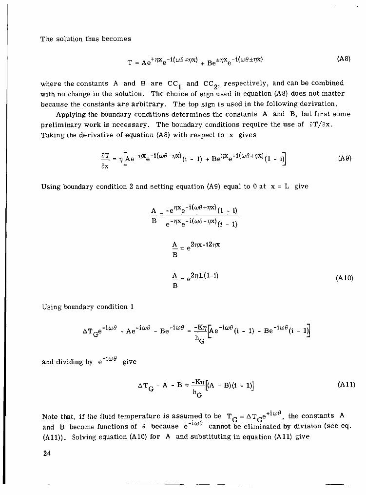
The solution thus becomes

where the constants A and B are CC1 and CC2, respectively, and can be combined with no change in the solution. The choice of sign used in equation (A8) does not matter because the constants are arbi t rary. The top sign is used in the following derivation.

preliminary work is necessary. The boundary conditions require the use of aT/ax. Taking the derivative of equation (A8) with respect to x gives

Applying the boundary conditions determines the constants A and B, but first some

Using boundary condition 2 and setting equation (A9) equal to 0 at x = L give

A - - - e2qx-i2ux B

A - e277L(1-i) B - -

Using boundary condition 1

-iwe give and dividing by e

A T G - A - B =*[(A 1. - B)(i - 11 “G

Note that, if the fluid temperature is assumed to be TG = ATGe+iWB, the constants A and B become functions of 0 because e cannot be eliminated by division (see eq. (All)). Solving equation (A10) fo r A and substituting in equation (Al l ) give

24

Collecting t e rms and solving f o r B give

Rearranging this equation gives

Changing to the polar form gives

B = ATG

-Kg [1 - e2qL(cos 2 q ~ - i sin 2 q ~ j j + + e2qL(cos 2 q ~ - i sin 2 q ~ 4 + i 9 - e'qL(cos 277~ - i sin 2 . ~ 4

hG hG

Collecting the t e r m s in the denominator on i gives

The following trigonometric substitution can be made in the previous equation:

25

where

Then

ATG

1 - 3 + Ee2qL(cos eG cos 2qL - sin cG sin 2qL) + i + e2qLE(-cos cG sin 2qL - sin cG COS 2qL) 1 B =

hG

This equation simplifies to

AT,

1 - 9 + e2qLE hG

The complex numbers must be in the numerator so that the phase shift accounts for the resistance of the boundary layer hG. This requirement will become apparent. T o put the complex numbers in the numerator, divide the denominator into the numerator in the previous equation for B by multiplying each number by the conjugate of the denominator. The following equation results:

-it AT-e B = cr --

- e2qLE sin(cG + 2vL) I’ From equation (AlO), A is

277 Le -i( 5 +2q L) (A 13)

hTGe - A =2 -

- 5 + e2qLE cos(€ + 2qL) + 5 - e2qLE sin(eG + 2qL) i F G 1‘ I’ 26

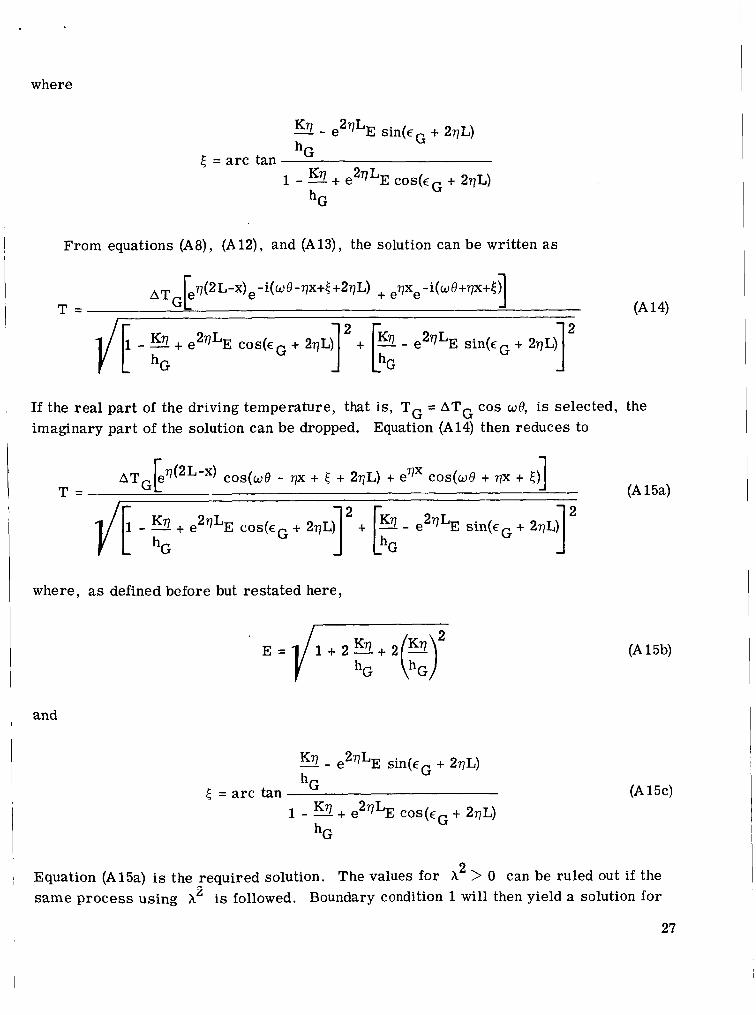
where

r

3 - e2qLE sin(EG + 2qL) hG 4 = a r c tan

1 - 9 + e2qLE + 2qL) hG

+ [F - e2qLE sin(EG + 2qL) 1" - 2

From equations (A8), (A 12), and (A 13), the solution can be written a s

q(2L-~)~-i(wO-qx+[+2qL) + ,gx,-i(d+qx+[) T = 1 (A 14)

f - 2 + e2qLE + 2qL)

If the rea l par t of the driving temperature, that is, TG = A T G cos we, is selected, the imaginary par t of the solution can be dropped. Equation (A14) then reduces to

r 1

] + [: - e2qLE sin(cG + 27L) l2 1/E - + e2r7LE + 2qL)

where, as defined before but restated here,

E = iw and

3 - e2qLE sin(EG + 27L) hG E = a r c tan

(A 15b)

(A 15c) 1 - 3 + e2qLE cos(cG + 2qL)

hG

2 Equation (A15a) is the required solution. The values for X > 0 can be ruled out if the s a m e p rocess using A' is followed. Boundary condition 1 will then yield a solution for

27

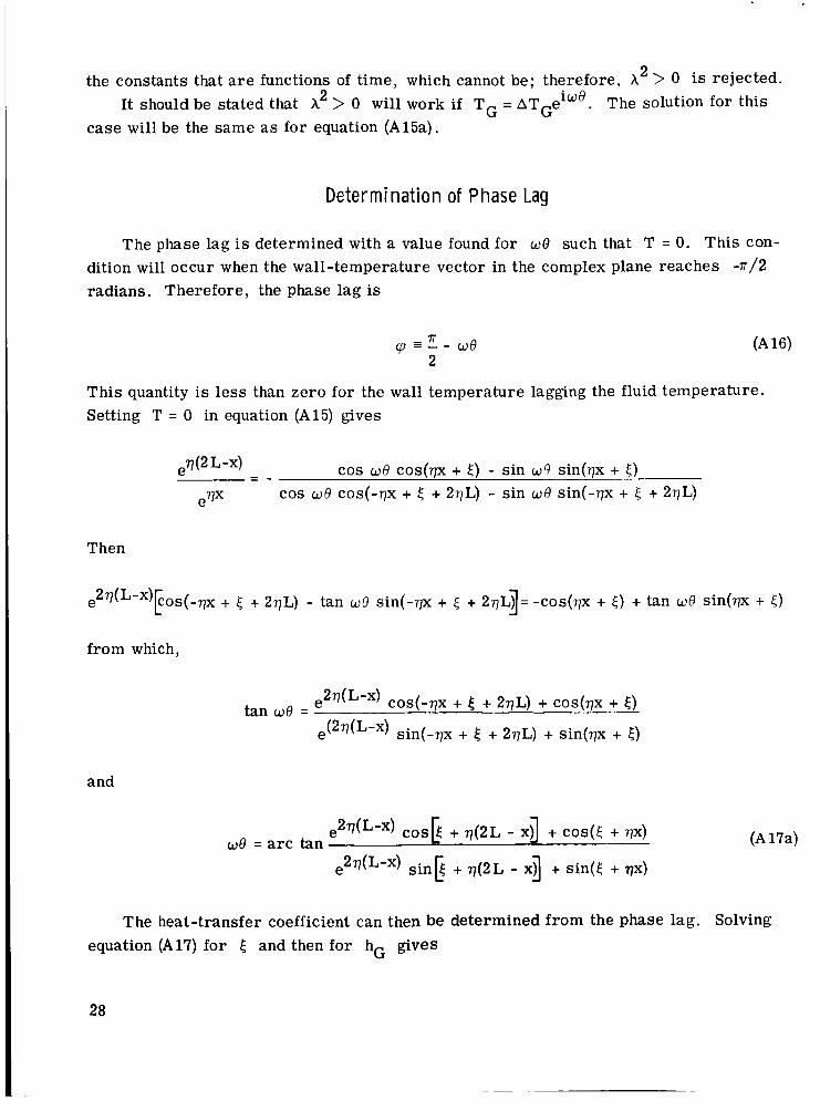
2 the constants that are functions of t ime, which cannot be; therefore, h > 0 is rejected.

case will be the same as for equation (A15a).

2 It should be stated that h > 0 will work if TG = ATGeiwe. The solution for this

Determination of Phase Lag

The phase lag is determined with a value found for we such that T = 0. This condition will occur when the wall-temperature vector in the complex plane reaches -7r/2 radians. Therefore, the phase lag is

This quantity is less than zero for the wall temperature lagging the fluid temperature. Setting T = 0 in equation (A15) gives

e q(2L-x) - cos w e cos(qx + t ) - sin w9 sin(qx + t ) cos we cos(-qx + 5 + 2qL) - sin we sin(-qx + 5 + 2qL)

_ - eqx

Then

from which ,

e 2q(L-x) cos(-qx + 5 + 2qL) + cos(qx + - 5 ) tan we = e ( 2 q ( L - ~ ) sin(-qx + 5 + 2 7 ~ ) + sin(qx + 5 )

and

e 2dL-x) c0.k + q(2L - x i + cos(( + qx) we = a r c tan

e2q(L-X) s i n k + q ( 2 ~ - x] + sin([ + qx)

(A 17a)

The heat-transfer coefficient can then be determined f rom the phase lag. Solving equation (A17) f o r 5 and then for hG gives

28

'TGX) [cos 5 cos 7 ( 2 ~ - x) - sin 5 s i n q ( 2 ~ - x)] + cos 5 cos 77x - sin 5 sin 7p we = a r c tan e e '~(L-x) [sin 5 cos q ( 2 ~ - x) + cos 5 sin q ( 2 ~ - x)] + sin 5 cos rpr + cos 5 sin

s in qx - - tan 5 -- e 2q(L-x)[1 - tan 5 tan q ( 2 ~ - x)] +

e 2q(L-x)[tan 5 + tan q ( 2 ~ - xu + tan < -- cos qx

cos qx

0 0 = a r c tan cos q(2L - x) cos q(2L - x) s in qx + ---

cos q(2L - x) cos q(2L - x)

From equation (A 16),

where cp is l e s s than zero f o r the wall temperature lagging the fluid temperature, and

tan w e = tan(: - cp)

tan we = cot (D

The foregoing expression is used in equation (A17a) to write

+ --j+ cos qx e 2 ~ ( L - x ) tan n ( 2 ~ , - x) + - sin qx cos q(2L - x) cos q(2L - x)

Solving fo r tan 5 gives

29

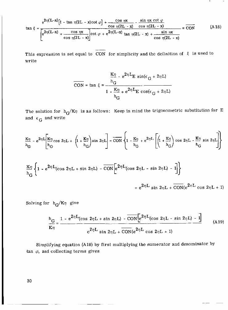
- tan 77(2~ - x)cot cp] + 7 7 ~ - sin qx cot cp - E CON (A 18) cos 77(2L - x) cos q(2L - x)

'Os qx cot cp + e 277UJ-x) tan 77(2L - x) + sin nx cos q(2L - x) 1 cos q(2L - x)

tan 5 = 2dL-X) +

This expression is set equal to CON for simplicity and the definition of 5 i s used to write

K17 -- - e2yLE sin(cG + 2yL)

- hG CON = tan 5 = 1 - f(rl+ e2qLE + 2yL)

hG

The solution for h d K y is as follows: Keep in mind the trigonometric substitution for E and c G and write

9 1 - e (cos 2 q ~ + s in 2 7 ~ ) - CON e2qL(cos 277~ - sin 277~) - 1 hG { 2 ' L -[ I>

= e2yL sin 2yL + CON(e277L cos 2yL + 1)

Solving for hG/Kq give

e2qL s in 2yL + CON(e2yL cos 2yL + 1)

Simplifying equation (A 18) by first multiplying the numerator and denominator by tan q, and collecting t e rms gives

30

'Os qx t a n q

sin qx 1 + -- 217(L,-x)

cos q(2L - x) cos T(21, - x)

cos q(2Lt - x

sin "-1 + [. -- -p2v(L-x) tan ~ Q L - x) + - CON = --

COS 77X ] + e 2"L-x)pn n ( 2 ~ - x) + cos v(2L - x)

Defining

2dL-X) + cos l)x

e 2 q ( L - ~ ) tan q ( 2 ~ - x) + --

e cos q(2L - x) A(x,L,q) = -

sin qx cos q(2L - x)

e 2q(L-x) cos q(2L - x) + cos qx

e 2v(L-x) sin q ( 2 ~ - x) + sin qx A(x, L,q) E --

Then

Equations (A19) and (A20) are the solutions presented in the text. For x = L,

A(x, L,q) = cot qL

tan cp - tan qL CON = -- 1 + tan cp tan qL

-- CON = tan(q - qL)

31

REFERENCES

1. Anderson, Bernhard H. : Improved Technique fo r Measuring Heat Transfer Coeffi- cients. Proceedings of the Fourth AFBMD/STL Symposium, Advances in Ballistic Missile and Space Technology. Vol. 2. Cnarles T . Morrow, ed . , Pergamon Press, 1960, p. 352.

Cyclic Temperature Variations. Heat Transfer and Fluid Mechanics Institute, 2. Bell, J . C. ; and Katz, E . F. : A Method for Measuring Surface Heat Transfer Using

ASME, 1949, pp. 243-254. 3. Wylie, Clarence R. , Jr. : Advanced Engineering Mathematics. Second e d . , Mc-Graw-

Hill Book Co. , Inc . , 1960.

32 NASA-Langley, 1968 - 33 E-4343

If Undeliverable (Section 1: postal Manual ) Do Nor Ret

‘The aeronautical and space activities of the United States shall be conducted so as to contribute . . . to the expansion of human knowledge of phenontena in the atmosphere and space. The Administration shall provide for the widest practicable and appropriate dissemination of ilsfornzation concerning its activities and the results thereof.”

-NATIONAL AERONAUTICS AND SPACE ACT OF 1958

AS TIFIC AND TECHNICAL PUBLICATIONS

REPORTS: Scientific and mation considered important, a lasting contribution to existing

knowledge.

TECHNICAL NOTES: Information less broad in scope but nevertheless of importance as a contribution to existing knowledge.

TECHNICAL MEMORANDUMS: Information receiving limited distribution because of preliminary data, security classifica- tion, or other reasons.

CONTRACTOR REPORTS: Scientific and technical information generated under a NASA entract or grant and considered an important : tontribution to existing knowledge.

TECHNICAL TRANSLATIONS: Information published in a foreign language considered to merit NASA distribution in English.

SPECIAL PUBLICATIONS: Information derived from or of value to NASA activities. Publications include conference proceedings, monographs, data compilations, handbooks, sourcebooks, and special bibliographies.

TECHNOLOGY UTILIZATION PUBLICATIONS: Information on technology used by NASA that may be of particular interest in commercial and other non-aerospace npp!icshns. ?ublica~icns indude Tech Briefs, Technology Utilization Reports and Notes, and Technology Surveys.

Details on the availability of these publications may be obtained from:

SCIENTIFIC AND TECHNICAL INFORMATION DIVISION

NATiaNAL AtKuNAui iLa MIAU 3 r n L c M U M I I Y I ~ I K A I I U I Y

Washington, D.C. PO546

- - - L . ~ m s - n m m A L I ~ r n n ~ e w A A L A B ~ B I ~ ~ T ~ A T B - L B

determination of convective heat … of convective heat-transfer coefficients on adiabatic walls...

Documents