determinants of internal migration in korea

This article was downloaded by: [University of Strathclyde]On: 06 October 2014, At: 19:52Publisher: RoutledgeInforma Ltd Registered in England and Wales Registered Number: 1072954Registered office: Mortimer House, 37-41 Mortimer Street, London W1T 3JH, UK

Journal of East and West Studies:Perspectives on East AsianEconomies and IndustriesPublication details, including instructions for authors andsubscription information:http://www.tandfonline.com/loi/rger19

Determinants of Internal Migrationin KoreaKong Kyun RoPublished online: 19 Aug 2009.

To cite this article: Kong Kyun Ro (1976) Determinants of Internal Migration in Korea, Journalof East and West Studies: Perspectives on East Asian Economies and Industries, 5:2, 63-80,DOI: 10.1080/12265087609431845

To link to this article: http://dx.doi.org/10.1080/12265087609431845

PLEASE SCROLL DOWN FOR ARTICLE

Taylor & Francis makes every effort to ensure the accuracy of all the information(the “Content”) contained in the publications on our platform. However, Taylor& Francis, our agents, and our licensors make no representations or warrantieswhatsoever as to the accuracy, completeness, or suitability for any purpose of theContent. Any opinions and views expressed in this publication are the opinions andviews of the authors, and are not the views of or endorsed by Taylor & Francis. Theaccuracy of the Content should not be relied upon and should be independentlyverified with primary sources of information. Taylor and Francis shall not be liablefor any losses, actions, claims, proceedings, demands, costs, expenses, damages,and other liabilities whatsoever or howsoever caused arising directly or indirectly inconnection with, in relation to or arising out of the use of the Content.

This article may be used for research, teaching, and private study purposes. Anysubstantial or systematic reproduction, redistribution, reselling, loan, sub-licensing,systematic supply, or distribution in any form to anyone is expressly forbidden.Terms & Conditions of access and use can be found at http://www.tandfonline.com/page/terms-and-conditions

http://www.tandfonline.com/loi/rger19

http://www.tandfonline.com/action/showCitFormats?doi=10.1080/12265087609431845

http://dx.doi.org/10.1080/12265087609431845

http://www.tandfonline.com/page/terms-and-conditions

http://www.tandfonline.com/page/terms-and-conditions

Determinants of Internal Migration In Korea

Kong Kpun Ro

I. Introduction

Tliere is a growing recognition that analysis of the economic inter-actions among sectors is the most promising approach to the study of development. Among the intersectoral relationships, the “rate of industrial labor absorption in excess of the rate of population growth” has been said to be the “criterion of success” in the development effdrt.1) The objective of this study is to examine economic factors which influence the rural-urban migration which accompanies industrial labor absorption.

The basic premise of this study is that migration is a decision of each individual to maximize the expected return to investment in human capital.*) It is assumed that the “efficiency” in migration3) is directly related the rural- urban differences in the expected presznt value of this investment. Based on this assumption, we propose to seek and examine the factors which influence the rural-urban differences in these expected values as perceived by the migrants and wouId-be migrants.

The framework of analysis is that of two-sectors: the urban, manufacturing and “labor recipient” sector and the rural, agricultural aad “labor donor” sector. The unit of observation is the kun or county (major cities have a separate status and are not within any kun). The destinations of individual migrants

1) Gustav Ranis, “Allocation Criteria and Population Growth,” American Economic Review, Vol. 53, No. 2 (May 1963). p. 623.

2) The human capital approach to migration has been initiated to my best knowledge, by Larry A. Sjaastad, “The Costs and Returns of Human Migration,” Journal of PoliticaI Econonnr, Vol. 70, No. 5, Part 2 (Supplement: October 1962), pp. 80-93. More recent empirical studies based on this approach are reported in Samuel Bowles, “Migration as Investment: EmpiricM Tests of Human Investment Appoach to Geographical Mobility,” Review of Economics and Statistics, Vol. 52, No. 4, November 1970, pp. 356-362; M. J. Bowman and R. Myers, “Schooling Experience and Gains and Losses in Human Capital Through Migration,” Journal of the American Statistical Association, Vol. 62, September 1967; and Gene Laber and R. X. Chase, “Interprovincial Migration in Canada as 8 Human Capital Decision,” Journal of Political Economy, Vol. 79, No. 4, July/August

3) The ratio ofnet migration to gross migration has been considered to be an indicator of the efficiency of migration. See H. S. Shyrock, Jr. “The Efficiency of International Migration in the United States” in Proccedings, international Conference, Vienna, 1959, pp- 685- 685-94; and Aba Schwartz, “On Efficiency of Migration,“ Journh of Human Resources. Vol. VI. No. 2 (Spring 1971), pp. 193-205.

63

1971, pp. 795-804.

Dow

nloa

ded

by [

Uni

vers

ity o

f St

rath

clyd

e] a

t 19:

52 0

6 O

ctob

er 2

014

Journal of East and West Studies (Vol V. 2)

from kuns are unknown. By necessity, therefore, the urban sector is treated as a single unit into which move all migrants, excluding those who move from kun to kun. The empirical testing of our model consists of examining how the variations in the rate of net migration among 169 kuns in South Korea in 1970 are related to the variations among kuns in those factors which are theorized to influence rural-urban diffxences in the expected returns to investment in human capital.

11. Model

We present two models, an aggregate model and an individual behavior model. The macro-model is presented to show how factor mobility is induced by the difference in marginal revenue product of labor and capital bztween the urban and rural sectors in the context of the aggregate production function of the economy. The micro-model is presented to show how this induced factor mobility is the result of utility maximization behavior of individuals. The macro- model is presented simply to provide a framework of reference and it is the micro-model only which is tested with the data in this study.

Thz macro underpinning of our model may be presented as follows:

where Y/Y is the rate of growth of total output measured in money; SA and S-tr arc shares of the agricultural sector and manufacturing secotr

in the total output; QA/QA and Qx/QM are rates of growth of agricultural goods and manu-

factured goods; P.11 and P,i are prices of manufactured goods and agricultural goods; ilg/aKJf and are marginal physical products of capital in the manu-

TK and Tt are rates of transfir of capital and labor between the two sectors; K/Y and L/Y are capital-output and labor-output ratios; and finally

facturing sector and in th:: agricultural sector;

4) This formulation of the model has been patterned after that by Sharrnan Robinson, which we have found to be most elucidating for our purpose at hand. See Sharman Robinson, “Sources of Growth in Less Developed Countries: A Cross-Section Study,” Quarterly Joiirnal of Econo~nics, Vol. 85, No. 3, August, 1971, pp. 390-405. Like most growth models appearing in recent literature, his model is presented in the tradition of the aggregate production functions of Solow and Swan. The derivatio nof equation 1 is presented in Appendix A.

64

Dow

nloa

ded

by [

Uni

vers

ity o

f St

rath

clyd

e] a

t 19:

52 0

6 O

ctob

er 2

014

Determinants of Internal hligration in Korea

ag/aLAI and 8flaL~ are marginal physical products of labor in the manufacturing sector and in the agricultural sector.

The expression [P.v g/aLx - PA -.G;flaL~] is the difference in the marginal revenue product of labor between the two sectors. It is this which induces labor movement. The above aggregate model demonstrates that migration is an adaptive process to disequilibrium in the economy, and that migration will continue until the disequilibrium disappears. . In our micro model, the induced labor movement is seen as the sum result of individual decisions to exploit economic disequilibrium. We assume that individuals make decisions as if they considered the benefits and cost of moving in the context of a general investment problem, and that rational decision calls for maximizing the discounted present value of the expected net real income stream over a would-be migrant’s planning time horizon. In this study the net real income is defined as pecuniary income adjusted by the difference in rural and urban cost of living, plus psychic income. Payment in kind, or concealed income, in rural areas should be considered as a factor lowering the rural cost of living.

Among several migration models5) examined, the one formulated by TodaroG) is found to be most useful for our study and our micro model adopts many of its distinctive features.

Let EVu(t) be the discounted value of the expected real income stream in urban areas and EYR(t) that in rural areas. Then,

where Wu(t) represents urban wage rate in period t , r is the discount rate which is

assumed to bz constant over time, Pu(t) is the probability of finding a job in urban areas in period t , ( t ) is the urban price deflator reflecting the urban-rural difference in the cost of living in period t , and a(t) is a scalar proxy for positive pyschic income of city life in period t.

The symbols in equation (3) are self-explanatory: R represents rural. Our ’ behavioral model of migration now can be shown as:

5) See S. Bowles; M. Bowman and R. Myers; and G. Leber and R. Chase: op. cit. (in f. n. 2).

6) Michael P. Todaro in “A Model of Labor Migration and Urban UnempIoyment in Less Developed Countries,” An:ericutz Econoniic Review, Vol. 69, No. 1 March 1969 pp. 138- 48.

65

Dow

nloa

ded

by [

Uni

vers

ity o

f St

rath

clyd

e] a

t 19:

52 0

6 O

ctob

er 2

014


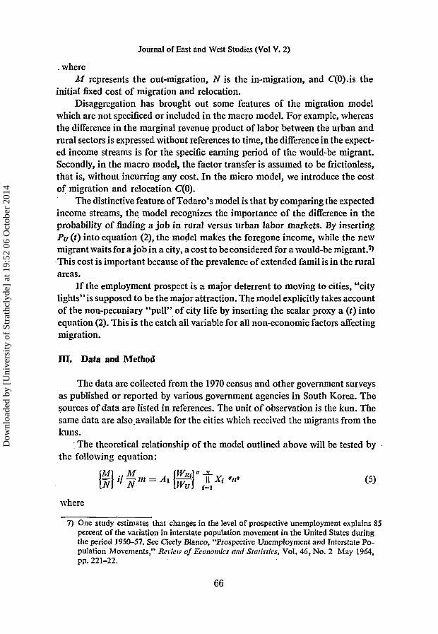
. where ikf represents the out-migration, N is the in-migration, and C(O).is the

initial fixed cost of migration and relocation. Disaggregation has brought out some features of the migration model

which are not specificed or included in the macro model. For example, whereas the difference in the marginal revenue product of labor between the urban and rural sectors is expressed without references to time, the difference in the expected income streams is for the specific earning period of the would-be migrant. Secondly, in the macro model, the factor transfer is assumed to be frictionless, that is, without incurring any cost. In the micro model, we introduce the cost of migration and relocation C(0).

The distinctive feature of Todaro’s model is that by comparing the expected income streams, the. model recognizes the importance of the difference in the probability of finding a job in rural versus urban labor markets. By inserting Pu (f) into equation (2), the model makes the foregone income, while the new migrant waits for a job in a city, a cost to be considered for a would-be migrant.’) This cost is important because of the prevalence of extended famil is in the rural areas.

If the employment prospect is a major deterrent to moving to cities, “city 1ights”is supposed to be the major attraction. The model explicitly takes account of the non-pecuniary “pull” of city life by inserting the scalar proxy a ( t ) into equation (2). This is the catch all variable for all non-economic factors affecting migration.

m. Data and Method

The data are collected from the 1970 census and other government surveys as published or reported by various government agencies in South Korea. The sources of data are listed in references. The unit of observation is the kun. The same data are also-available for the cities which received the migrants from the kuns.

: The theoretical relationship of the model outlined above will be tested by the following equation:

where

7) One study estimatesthat changes in the level of prospective unemployment explains 85 percent of the variation in interstate population movement in the United States during the period 1950-57. See Cicely Itlanco, “‘Prospective Unemployment and Interstate Po- pulation Movements,’’ Review of Ecorzoirzics and Sfafistics, Vol. 46, No. 2 May 1964, pp. 221-22.

66

Dow

nloa

ded

by [

Uni

vers

ity o

f St

rath

clyd

e] a

t 19:

52 0

6 O

ctob

er 2

014

Determinants of Internal Migration in Korea

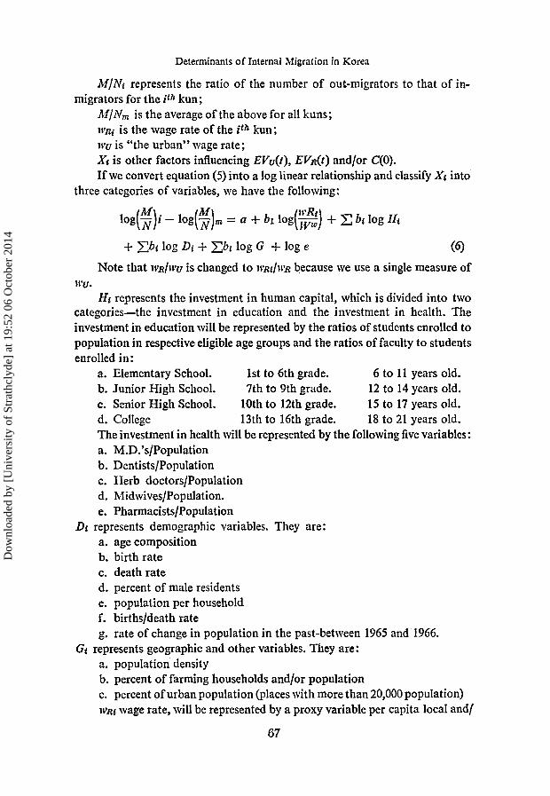
M/Nt represents the ratio of the number of out-migrators to that of in-

hif/N,,, is the average of the above for all kuns; I V R ~ is the wage rate of the i th kun; itv is “the urban” wage rate; Xr is other factors influencing EYu(t), EVa(t) and/or C(0). If we convert equation (5) into a log linear relationship and classify Xi into

migrators for the if” kun;

three categories of variables, we have the following:

+ Cbt log Dt f Cbt log G + log e (6) Note that IVR/WU is changed to w,t/m because we use a single measure of

WU. Ht represents the investment in human capital, which is divided into two

categories-the investment in education and the investment in health. The investment in education will be represented by the ratios of students enrolled to population in respective eligible age groups and the ratios of faculty to students enrolled in:

a. Elementary School. 1st to 6th grade. b. Junior High School. 7th to 9th grade. c. Scnior High School. 10th to 12th grade. d. College 13th to 16th grade. The investment in health will be represented by the following five variables: a. M.D.’s/Population b. Dentists/Population c. Herb doctors/Population d. Midwives/Population. e. Pharmacists/Population

a. age composition b. birth rate c. death rate d. percent of male residents e. population per household f. birthsldeath rate g. rate of change in population in the past-between 1965 and 1966.

a. population density b. percent of farming households and/or population c. percent of urban population (places with more than 20,000 population) itm wage rate, will be represented by a proxy variable per capita IocaI and/

6 to 11 years old. 12 to 14 years old. 15 to 17 years old. 18 to 21 years old.

Dt represents demographic variables. They are:

Gr represents geographic and other variables. They are:

67

Dow

nloa

ded

by [

Uni

vers

ity o

f St

rath

clyd

e] a

t 19:

52 0

6 O

ctob

er 2

014


or national tax revenues. .To the extent to which non-labor income, tax rates and their collection rates differ among kuns, the data will fail to-show the variation in wage rates among kuns accurately.

IV. Hypotheses

IV. 1. Income Differentials

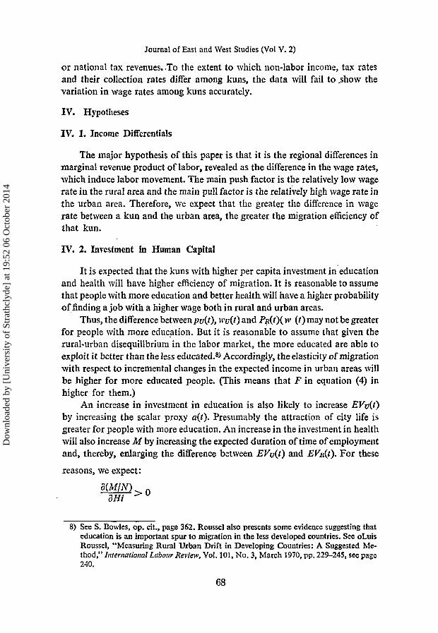
The major hypothesis of this paper is that i t is the regional differences in marginal revcnue product of labor, revealed as the difference in the wage rates, which induce labor movement. The main push factor is the relatively low wage rate in the rural area and the main pull factor is the reIatively high wage rate in the urban area. Therefore, we expect that the greater the difference in wage rate between a kun and the urban area, the greater the migration efficiency of that kun.

IV. 2. Investment in Human Capital

It is expected that the kuns with higher per capita investment in’education and health will have higher efficiency of migration. It is reasonable to assume that people with more education and better health will have a higher probability of finding a job with a higher wage both in rural and urban areas.

Thus, the difference bztwveenpu(t), wu(t) and PR(t)( 10 ( t ) may not be greater for people with more education. But it is reasonable to assume that given the rural-urban disequillbrium in the labor market, the more educated are able to exploit it better than the less educated.8) Accordingly, the elasticity of migration with respect to incremental changes in the expected income in urban areas will be higher for more educated people. (This means that F in equation (4) in higher for them.)

An increase in investment in education is also likely to increase EVu(t) by increasing the scalar proxy a(t). Presumably the attraction of city life is greater for people with more education. An increase in the investment in health will also increase M by increasing the expected duration of time of employment and, thereby, enlarging the difference between EVu(t) and EVn(t). For these

reasons, we expect:

8) See S. Boivles, op. cit., page 362. Roussel also presents some evidence suggesting that education is an important spur to migration in the less developed countries. See oLuis Roussel, “Measuring Rural Urban Drift in Developing Countries: A Suggested Me- thod,” Znternational Labour Review, Vol. 101, No. 3, March 1970, pp. 229-245, see page 240.

68

Dow

nloa

ded

by [

Uni

vers

ity o

f St

rath

clyd

e] a

t 19:

52 0

6 O

ctob

er 2

014

Determinants of Internal hligration in Korea

IV. 3. Demographic variables

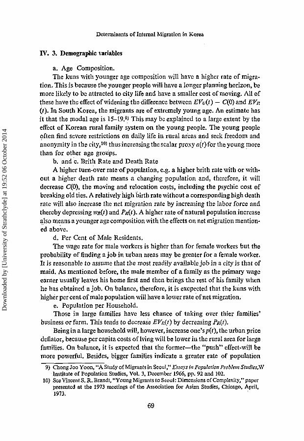
a. Age Composition. The Lams with younger age composition will have a higher rate of migra-

tion. This is because the younger people will have a longer planning horizon, be more likely to be attracted to city life and have a smaller cost of moving. All of these have the effect of widening the difference between EVv(t) - C(0) and EV, (t). In South Korea, the migrants are of extremely young age. An estimate has it that the modal age is 15-19.9) This may be explained to a large extent by the effect of Korean rural family system on the young people. The young people often find severe restrictions on daily life in rural areas and seek freedom and anonymity in the city,lO) thus increasing the scalar proxy o(t) for the young more than for other age groups.

b. and c. Brith Rate and Death Rate A higher turn-over rate of populztion, e.g. a higher brith rate with or with-

out a higher death rate means a changing population and, therefore, it will decrease C(O), the moving and relocation costs, including the psychic cost of breaking old ties. A relatively high birth rate without a corresponding high death rate will also increase the net migration rate by increasing the labor force and thereby depressing im(t) and P R O ) . A higher rate of natural population increase also means a younger age composition with the effects on net migration mentioned above.

d. Per Cent of Male Residents. The wage rate for male workers is higher than for female workers but the

probability of finding a job in urban areas may be greater for a female worker. It is reasonable to assume that the most readily available job in a city is that of maid. As mentioned before, the male member of a family as the primary wage earner usually leaves his home first and then brings the rest of his family when he has obtained a job. On balance, therefore, it is excpected that the kuns with higher per cent of male population will have a lower rate of net migration.

e. Population per Household. Those in large families have less chance of taking over thier families’

business or farm. This tends to decrease EF%(t) by decreasing PR(I). Being in a large household will, however, increase one’sp(t), the urban price

deflator, because per capita costs of lving will be lower in the rural area for large families. On balance, it is expected that the former-the “push” effect411 be more powerful. Besides, bigger families indicate a greater rate of population

9) Chong Joo Yoon, “AStudy of Migrants in Seoul,” Essays in Population Problem Studies,W Institute of Population Studies, Vol. 3, December 1966, pp. 92 and 102.

10) SeeVincent S. R. Brandt, “Young Migrants to Seoul: Dimcnsions of Complexity,” paper presented at the 1973 meetings of the Association for Asian Studies, Chicago, April, 1973.

69

Dow

nloa

ded

by [

Uni

vers

ity o

f St

rath

clyd

e] a

t 19:

52 0

6 O

ctob

er 2

014


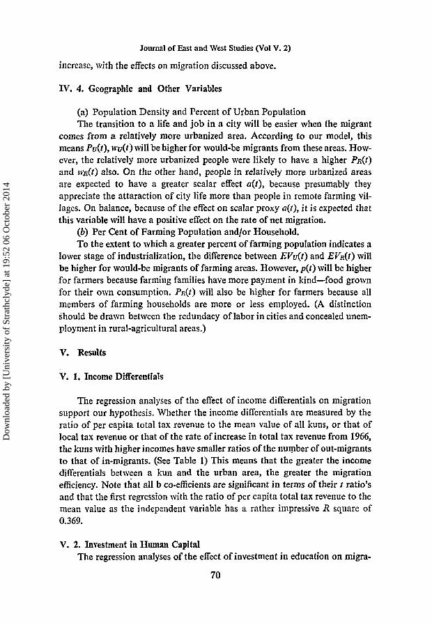
increase, with the effects on migration discussed above.

IV. 4. Geographic and Other Variables

(a) Population Density and Percent of Urban Population The transition to a life and job in a city will be easier when the migrant

comes from a relatively more urbanized area. According to our model, this means Pu(t), icu(t) will be higher for would-be migrants from these areas. How- ever, the relatively more urbanized people were likely to have a higher Px(t) and ~ m ( t ) also. On the other hand, people in relatively more urbanized areas are expected to have a greater scalar effect a(t), because presumably they appreciate the attaraction of city life more than people in remote farming vil- lages. On balance, because of the effect on scalar proxy a(t), it is expected that this variable will have a positive effect on the rate of net migration.

(b) Per Cent of Farming Population and/or Household. To the extent to which a greater percent of farming population indicates a

lower stage of industrialization, the difference between EVv(t) and E V R ( ~ ) will be higher for would-be migrants of farming areas. However, p ( t ) will be higher for farmers because farming families have more payment in kind-food grown for their own consumption. P R ( f ) will also be higher for farmers because all members of farming households are more or less employed. (A distinction should be drawn between the redundacy of labor in cities and concealed unemployment in rural-agricultural areas.)

V. Results

V. 1. Income DifferentiaIs

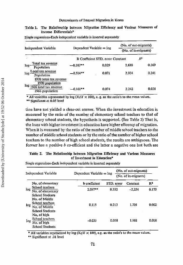
The regression analyses of the effect of income differentials on migration support our hypothesis. Whether the income differentials are measured by the ratio of per capita total tax revenue to the mean value of all kuns, or that of local tax revenue or that of the rate of increase in total tax revenue from 1966, the kuns with higher incomes have smaller ratios of the number of out-migrants to that of in-migrants. (See Table 1) This means that the grcater the income differentials between a kun and the urban area, the greater the migration efficiency. Note &at all b co-efficients are significant in terms of their t ratio’s and that the first regression with the ratio of per capita total tax revenue to the mean value as the independent variable has a rather impressive R square of 0.369.

V. 2. Investment in Human Capital The regression analyses of the effect of investment in education on migra-

70

Dow

nloa

ded

by [

Uni

vers

ity o

f St

rath

clyd

e] a

t 19:

52 0

6 O

ctob

er 2

014

Determinants of Internal Migratioe.ih Korea

Table 1. The Relationship between hllgration Efficiency and Various hleasures of Income Differentials*

Single regressions-Each independent variable is inserted separately

Independent Variable (No. of out-migrants) (No. of in-migrants)

Dependent Variable = log ~~ ~~ ~

B Coefficient STD. error Constant RZ

4.387** Total tax revenue log Population

-0.514** Local tax revenue log Powlation

0.039

0.071

2.618

2.924

0.369

0.241

19i0 total-tax revenue 1970 population

4.161** 0.074 2.242 0.028 log 1966 total tax revenue 1966 population

* All variables represented by log (XdX x loo), e. g. as the ratio's to the mean values. ** Significant at 0.05 level

tion have not yielded a clear-cut answer. When the investment in education is measured by the ratio of the number of elementary school teachers to that of elementary school students, the hypothesis is supported. (See Table 2) That is, the kuns with higher investment in education have higher efficency of migration. When it is measured by the ratio of the number of middle school teachers to the number of middle school students or by the ratio of the number of higher school teachers to the number of high school students, the results are ambiguous. The former, has a positive b co-efficient and the latter a negative one but both are

Table 2. The Relationship between Migration Efficiency and Various Measures of Investment in Education*



Dependent Variable = log

No. of elementary b coefficient STD. error Constant R2 School teachers

log NO. ofelementary School Students No. of Middle School teachers

log No. of Middle School Students No. of h k h School teachers

log No. of high

2.097* * 0.352 -2.254 0.175

0.115 0.213 1.705 0.002

-0.031 0.018 1.988 0.018

School Students

* All variables represented by log (Xt/X x loo), e.g. as the ratio's to the mean values. ** Significant at .01 level

71

Dow

nloa

ded

by [

Uni

vers

ity o

f St

rath

clyd

e] a

t 19:

52 0

6 O

ctob

er 2

014


not significant, and therefore cannot be taken seriously. An explanation may lie in the fact that many young pcople in the rural area leave for the urban area for high school and college education. Also the lack of high schools and/or colleges in the rural area serves as a push factor for rural youths to seek higher education in cities.

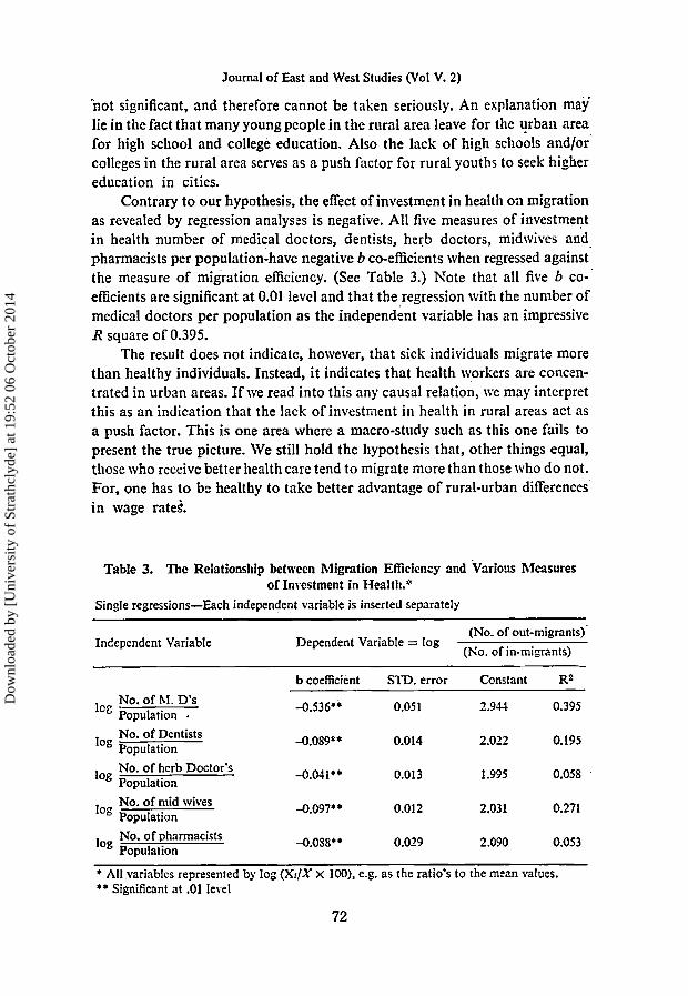
Contrary to our hypothesis, the effect of investmcnt in health oil migration as revealed by regression analyszs is negative. All fivc measures of investment in health number of medical doctors, dentists, herb doctors, midwives and- pharmacists per population-have negative b co-efficients when regressed against the measure of migration efficiency. (See Table 3.) Note that all five b co- efficients arc significant a t 0.01 level and that the regression with the number of medical doctors per population as the independent variable has an impressive R square of 0.395.

The result does not indicate, however, that sick individuals migrate more than healthy individuals. Instead, it indicates that health workers are concen- trated in urban areas. If we read into this any causal relation, we may interpret this as an indication that the lack of investment in health in rural areas act as a push factor. This is one area where a macro-study such as this one fails to present the true picture. W e still hold the hypothesis that, other things equal, those who receive better health care tend to migrate more than those who do not. For, one has to bc healthy to take better advantage of rural-urban differences in wage ratei.

Table 3. The Relationship betwcn hligration Efficiency and Vario?~s hlcasures of Investment in Health."


Independent Variable (No. of out-migrants)-

Dependent Variable = log (No. of in-migrants)

No. of hl. D's

No. of Dentists log Population . log Population

No. of herb Doctor's log Population

No. of mid wives log Population

No. of pharmacists log Population

b coefficient STD. error Constant R2

-0.536'4 0.051 2.93-1 0.395

-0.089** 0.0 14

-O.OJl** 0.013

-0.097,' 0.012

-0.058** 0.029

2.012 0.195

1.995 0.058

2.031 0.271

2.090 0.053

* All ,variables represented by log (Xr/X X IOO), e.g. as the ratio's to the mean values. ** Significant at .01 level

72

Dow

nloa

ded

by [

Uni

vers

ity o

f St

rath

clyd

e] a

t 19:

52 0

6 O

ctob

er 2

014

DMrniinants of Internal Migration in Korea

1'. 3. Demographic Variables

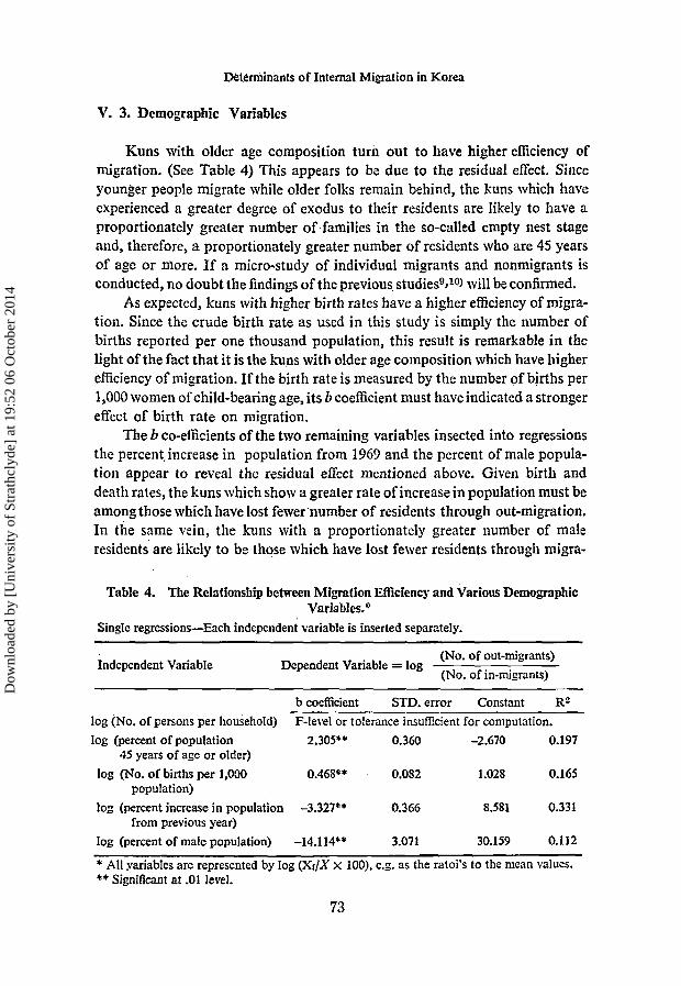
Kuns with older age composition turn out to have higher efficiency of migration. (See Table 4) This appears to be due to the residual effect. Sirice younger people migrate while older folks remain behind, the kuns which have experienced a greater degree of exodus to their residents are Iikely to have a proportionately greater number of families in the so-called empty nest stage and, therefore, a proportionately greater number of residents who are 45 years of age or more. If a micro-study of individual migrants and nonmigrants is conducted, no doubt the findings of the previous studies9P)) will be confirmed.

As expected, kuns with higher birth rates have a higher efficiency of migration. Since the crude birth rate as used in this study is simply the number of births reported per one thousand population, this result is remarkable in the light of the fact that it is the kuns with older age composition which have higher efficiency of migration. If the birth rate is measured by the number of births per 1,000 womeit of child-bearing age, its b coefficient must have indicated a stronger effect of birth rate on migration.

The b co-efirients of the two remaining variables insected into regressions the percent increase in population from 1969 and the percent of male population appear to reveal the residual effect mentioned above. Given birth and death rates, the kuns which show a greater rate of increase in population must be among those which have lost fewverxumber of residents through out-rnigration. In the same vein, the kuns with ;1 proportionately greater number of male residents are likely to be those which have lost fewer residents through migra-

Table 4. The Relationship between Migration Efficiency and .Various Demographic Variables. *

Single regressions-Each independent variable is inserted separztely.



b coefficient STD. error Constant Ra log (No. of persons per household) log (percent of population 2.305** 0.360 -2.670 0.197

45 years of age or older) log (No. of births per 1,090 0.468** o.os2 1.02s 0.165

log (percent increase in population -3.327** 0.366 8.581 0.331

F-level or tolerance insuRcient for computation.

population)

from previous year) log (percent of male population) -14.114** 3.071 30.159 0.112

* All yariables are represented by log ( X t / X x loo), e.g. as the ratoi's to the mean values. *+ Significant at .01 level.

73

Dow

nloa

ded

by [

Uni

vers

ity o

f St

rath

clyd

e] a

t 19:

52 0

6 O

ctob

er 2

014


tion, because the heads of households are likely to migrate first. Geographic variables :

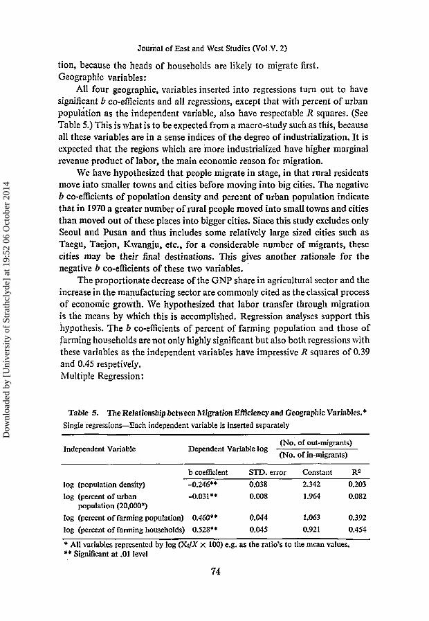
All four geographic, variables inserted into regressions turn out to have significant b co-efficients and a11 regressions, except that with percent of urban population as the independent variable, also have respectable R squares. (See Table 5.) This is what is to be expected from a macro-study such as this, because all these variables are in a sense indices of the degree of industrialization. I t is expected that the regions which are more industrialized have higher marginal revenue product of labor, the main economic reason for migration.

Wc have hypothesized that people migrate in stage, in that rural residents move into smaller towns and cities before moving into big cities. The negative b co-efficients of population density and perc:nt of urban population indicate that in 1970 a greater number of rural people moved into small towns and cities than moved out of these places into bigger cities. Since this study excludes only Seoul and Pusan and thus includes some relatively large sized cities such as Taegu, Taejon, Kwangju, etc., for a considerable number of migrants, these cities may be their final destinations. This gives another rationale for the negative b co-efficients of these two variables.

The proportionate decrease of the GNP share in agricultural sector and the increase in the manufacturing sector are commonly cited as the classical process of economic grokh. We hypothesized that labor transfer through migration is the means by which this is accomplished. Regression analyses support this hypothesis. The b co-efficients of percent of farming population and those of farming households are not only highly significant but also both regressions with these variables as the independent variables have impressive R squares of 0.39 and 0.45 respetively. Multiple Regression:

Table 5. The Relationship between Migration Efficiency and Geographic Variables.* Single regressions-Each independent variable is inserted separately


Dependent Variable log

b coefficient STD. error Constant R2 log .(population density) -0.246** 0.038 2.342 0.203 log (percent of urban -0.031** 0.008 1.964 0.082

population (20,000*) log (percent of farming population) 0.460** 0.044 1.063 0.392 log (percent of farming households) 0.528** 0.045 0.921 0.454

* All variables represented by log (Xt /X X 100) e.g. as the ratio’s to the mean values. ** Significant at .01 level

74

Dow

nloa

ded

by [

Uni

vers

ity o

f St

rath

clyd

e] a

t 19:

52 0

6 O

ctob

er 2

014


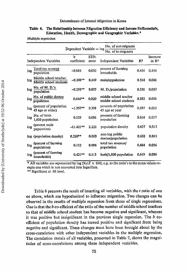
Table 6. The Relationship between Migration Efficiency and Income Defferentials, Education, Health, Demographic and Geographic Variables.*

Multiple regression

No. of out-migrants No. of immigrants


b STD. Increase Independent Variables coefficient error Independent Variables R2 in Ra

Total tax revenue percent of farming o.454 o.454 log population 0*050 households

-0.248** 0.149 male/oppulation 0.514 0.061 Middle school teacher log Middle school students

-0.298** 0.075 M. D./population 0.551 0.037 No. of M. D.'s log population

No. of public doctor middle school teacher o,582 o.031 log population oB44** Oao20 middle school students

0.597 0.015 (percent of population percents of population log 45 age or older)

percents of farming . 0.614 0.017 No. of birth log 1,000 population 0*139 O*OS6 population

-11.421** 2.221 population density 0.627 0.013 (percent male log population)

0.638 0.011 non-log public log (population density) 0.210** 0.060 doctor,population

0.664 0.006 (percent of farming total tax revenue/ log population) 0.'12 O*Og6 population

(percent Of farming 0.421** 0.113 both/1,000 population 0.649 0.006 log households)

* All variables are represented by log (Xt/.?? x IOO), e.g. as the ratio'; to the m-an values ex- cepts one which is not converted into logarithm. ** Significant at .05 level.

-1.357** 0.398 45 age or year

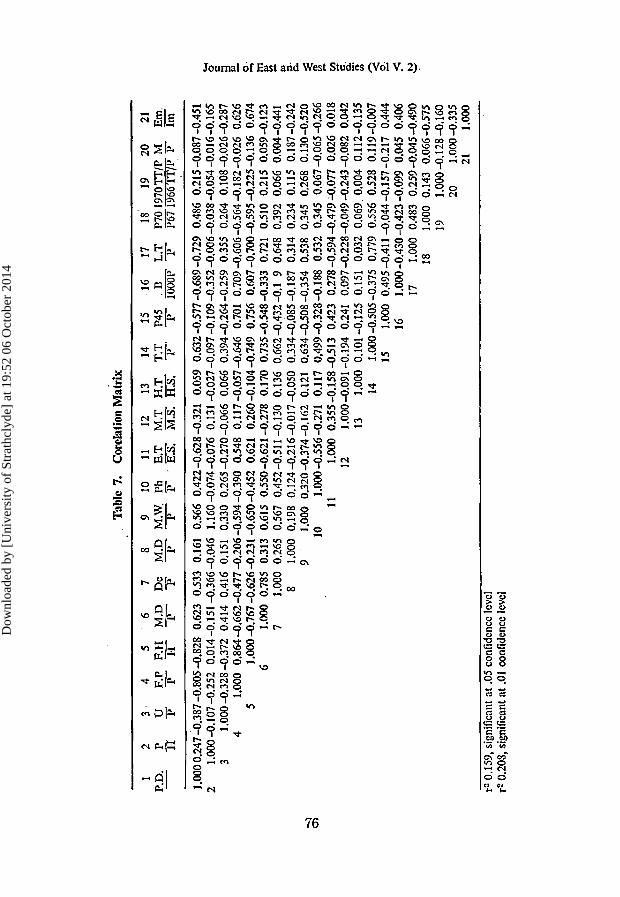
Table 6 presents the result of inserting all variables, with the t ratio of one o r above, which are hypothesized to influence migration. Two changes can be observed in the results of multiple regression from those of single regressions. One is that the b co-efficient of the ratio of the number of middle school teachers to that of middle school student has become negative and significant, whereas it was positive but insignificant in the previous single regression, The b coefficient of population density has turned positive and significant from being negative and significant. These changes must have been brought about by the cross-correlation with other independent variables in. the multiple regression. The correlation matrix of all variables, presented in Table 7, shows the magni- tudes of cross-correlations among these independent variables.

75

Dow

nloa

ded

by [

Uni

vers

ity o

f St

rath

clyd

e] a

t 19:

52 0

6 O

ctob

er 2

014

Tabl

e 7.

C

orela

tion

Mat

rix

1 2

3 4

5 6

7 8

9 10

11

12

13

14

15

16

17

18

19

20

21

P.D.

P u

rx FZ

MZ DC

M.D

M

.W.

pi1

E.T

M.T

H

.T

T.T

r45

B

L.T

P~

O~

~~

OT

T/P

M

~m

H

P'

1' H

I' T

T

TF

E.S

;Mg

;FiX

T

T

i3G

GF

-T

M1-F

Im

-

1.000

0.24

7 -0

.387

-0.80

5 -0

.828

0.

623

0.53

3 0.

161

0.566

0.

422

-0.6

28 -

0.32

1 0.0

59

0.63

2 -0

.577

-0.6

89 -

0.729

0.4

86

0.21

5 -0

.087

-0.45

1 2

1.00

0-0.

107-

0.25

2 0.

014-

0.15

1 -0

.366

-0.0

46

1.16

0 -0.

074-

0.07

6 0.

131

-0.0

27-0

.097

-0.1

09-0

.352

-0.0

06-0

.038

-0.0

54-0

.016

-0.1

65

2

3 1,

000-

0.32

8 -0

.372

0.

414

0.41

6 0.

151

0.33

0 0.

265

-0.2

70-0

.066

0.

066

0.39

4-0.

264-

0.25

9 0.

355 0.2G4

0.10

8 -0

.026

-0.2

87

4 1.

000

0.86

4-0.

662-

0.47

7 -0

.206

-0.5

94

-0.3

90

0.54

8 0.

117

-0.0

57 -0

.646

0.7

01

0.709

-0.

606

-0.5

64 -0

.182

-0.0

26

0.62

6 1.O

OO -

0.767

-0.6

26 -

0.23

1 -0

.650

-0.

452

0.62

1 0.

260

-0.1

04 -0

.749

0.

756

0.60

7 -0

.700

-0.

595

-0.2

25 -

0.136

0.

674

6 1.O

OO

0.785

0.3

13

0.61

5 0.

550-

0.62

1 -0

.278

0.

170

0.73

5-0.

548-

0.33

3 0.7

21

0.510

0.

215

0.05

9-0.

123

7 1.

000

0.26

5 0.5

67

0.45

2-0.

511

-0.1

30

0,13

6 0.

662-

0.43

2-0.

1 9

0.64

8 0.3

92

0.06

6 0.

004-

0.44

1 8

1.00

0 0,

198

0.12

4-0.

216-

0.01

7-0.

050

0,33

4-0.

085-

0.18

7 0.

314

0.23

4 0.

115

0.18

7-0.

242

9 1.

000

0.32

0 -0

.374

-0.

162

0.12

1 0.

634

-0.5

08 -

0.354

0.5

38

0.34

5 0.

268

0.13

0 -0

520

5 %

5

10

1.OOO

-0.55

6 -0

.271

0.1

17

0,49

9 -0

.328

-0.1

88

0.53

2 0.

345

0.06

7 -0.

065

-0.2

66

11

1.OOO

0.

355

-0.15

8 -0

.513

0.

423

0.27

8 -0

.594

-0.4

79 -

0.07

7 0.

026

0.01

8 12

1 .000 -

0.09

1 -0

.194

0.

241

0.09

7 -0

.228

-0.

049

-0.2

43 -

0.08

2 0.

042

13

1.00

0 0.

101

-0.1

25

0.15

1 0.

032

0.06

9 0.

004

0.11

2-0.

135

8 14

1.

000-

0.50

5-0.

375

0.779

0.5

56

0.52

8 0.

119

-0.0

07

15

1.OOO

0.

495

-0.4

11 -0

,044

-0.1

57 -0

.217

0.

444

3. 1 6

1 .O

OO -0

.430

-0.4

23 -

0,09

9 0.

045

0.40C

5

17

1,00

0 0.

483

0.25

3-0.

045-

0.49

0 18

1.

000

0.14

3 0.

066-

0.57

5 19

1.

000 -

0.12

8 -0

.160

20

1.

000-

0.33

5 21

1.O

OO

rz 0

.159

, sig

nific

ant a

t .0

5 co

nfid

cncc

lcvc

l r?

0.20

3, s

igni

fican

t at .

01 c

onfid

cncc

lcvc

l

Dow

nloa

ded

by [

Uni

vers

ity o

f St

rath

clyd

e] a

t 19:

52 0

6 O

ctob

er 2

014


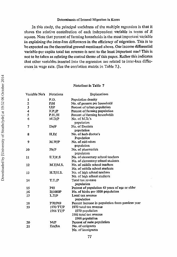
In this study, the principal usefulness of the multiple regression is that it shows the relative contribution of each independent variable in terms of R square. Note that percent of farming households is the most important variable in explaining the inter-kun differences in the efficiency of migration. This is to lx expected on the theoretical ground mentioned above. Our income differential variable-per capita total tax revenue-is next to the least important one! This is not to be taken as refuting the central theme ofthis paper. Rather this indicates that other variables inserted into the regression are related to inter-kun differences in wage rate. (See the corrlation matrix in Table 7.).

Variable No's Notations 1 P.D. 2 PIH 3 u/p 4 F.P./P 5 P.H./H 6 M.D/P

7 De/P

8 H.D/

9 M.\YJP

10 Ph/P

11 E.T/E.S

12 M.T/M.S.

13 H .T/H. S . 14 T.T./P

15 P.15 .I 6 B/1000P 17 L.T/P

18 P70/p69 19 1970 TTlp

1966 TT/P

20 hl/P 21 Em/Im

Notations in Table 7

Explanations Population density No. of persons per household Percent of urban population Percent of farming population Percent of farming households No. of M.D.'s '

population No. of Dentists

population No. of herb doctor's

Population No. of mid-wives

population No. of pharmacists

population No. of elementary school teachers No. of elementary school students No. of middle school teachers No. of middle school students No. of high school teachers No. of high school students Total tax revenue

Percent of population 45 years of age or older No. of births per lo00 population Local tax revenue

Percent increase in population from previous year 1970 total tax revenue

1970 population 1966 total tax revenue

1966 population Percent of male population No. of emigrants No. of immigrants

population

population

77

Dow

nloa

ded

by [

Uni

vers

ity o

f St

rath

clyd

e] a

t 19:

52 0

6 O

ctob

er 2

014


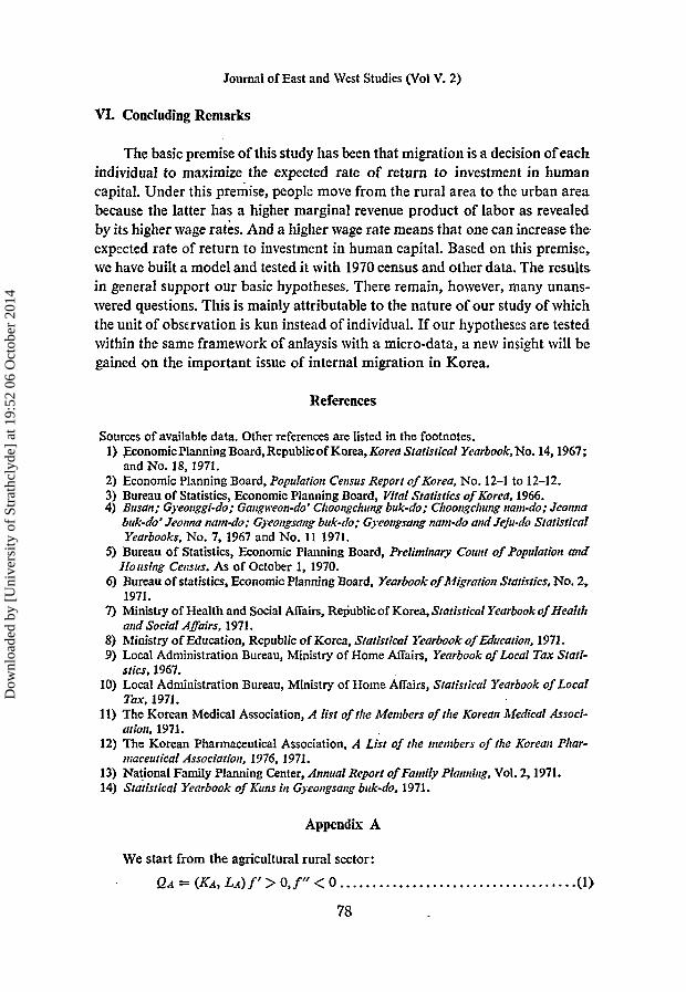
VI. Concluding Remarks

The basic premise of this study has been that migration is a decision of each individual to maximize the expected rate of return to investment in human capital. Under this premise, people move from the rural area to the urban area because the latter has a higher marginal revenue product of labor as revealed by its higher wage rates. And a higher wage rate means that one can increase the expected rate of return to investment in human capital. Based on this premise, we have built a model and tested it with 1970 census and other data. The results in general support our basic hypotheses. There remain, however, many unans- wered questions. This is mainly attributable to the nature of our study of which the unit of obscrvation is kun instead of individual. If our hypotheses are tested within the same framework of anlaysis with a micro-data, a new insight will be gained on the important issue of internal migration in Korea.

References

Sources of available data. Other references are listed in the footnotes. 1) EconomicPlanning Board, Republic of Korea, Korea Stutisticul Yearbook, No. 14,1967;

2 ) Economic Planning Board, Popillation Census Report of Korea, No. 12-1 to 12-12. 3) Bureau of Statistics, Economic Planning Board, Vital Statistics of Korea, 1966. 4) Busan; Gyeonggi-do; Gangweon-do' Choongcltitng buk-do; Clioorrgclriing num-do; Jeonna

buk-do ' Jeonna nanz-do; Gyeongsang buk-do; Gyeongsang nani-do and Jeju-do Statistical Yearbooks, No. 7, 1967 and No. 11 1971.

5) Bureau of Statistics, Economic Planning Board, Preliminary Count of Populution and

and No. 18,1971.

Hoiising Census. As of October 1, 1970. 6) Bureau of statistics, Economic Planning Board, Yearbook of M&utioiz Statistics, NO. 2,

1971. 7) Ministry of Health and Social Affairs, Republicof Korea, Statistical Yearbookof Health

8) Ministry of Education, Republic of Korea, Statistical Yearbook of Educaiion, 1971. 9) Local Administration Bureau, Ministry of Home Affairs, Yearbook of Local Tax Srari-

10) Local Administration Bureau, Ministry of Home Affairs, Stdtisticul Yearbook of Local

11) The Korean Medical Association, A list of the Members of the Korean Medical Associ-

12) The Korean Pharmaceutical Association, A List of the inentbers of the Korean Phar-

13) National Family Planning Center, Annual Report of Fantily Planning, Vol. 2,1971. 14) Statisrical Yearbook of Kuns in Gyeotrgsung buk-do, 1971.

and Social Agairs. 1971.

srics, 1967.

Tux, 1971.

utiott, 1971.

maceutical Association, 1976, 1971.

Appendix A

We start from the agricultural rural sector:

QA = (KA, LA)^'> 0 , y < 0 ...... ........ . ....... .... ...... ....( 1)

78

Dow

nloa

ded

by [

Uni

vers

ity o

f St

rath

clyd

e] a

t 19:

52 0

6 O

ctob

er 2

014


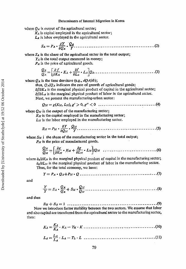
where QA is output of the agricultural sector; KA is capital employed in the agricultural sector; LA is labor employed in the agricultural sector.

dY ' P A aQA

S A = P A * - . 7.. .......................................... .(2)

where SA is the share of the agricultural sector in the total output; YA is the total output measured in money; PA is the price of agricultural goods.

-- af aLA . KA + - . LA]QA. ................................. ( 3 )

where QA is the time dervitave (e.g., dQA/dt); thus, QA/QA indicates the rate of growth of agricultural goods; aflaKA is the marginal physical product of capital in the agricultural sector; afldLA is the marginal physical product of labor in the agricultural sector. Next, we present the manufacturing-urban sector:

QJr = g(Kjr, Ljr), g' > 0, g" < 0 ............................... .(4)

where QJr is the output of the manufacturing sector; KJf is the capital employed in the manufacturing sector; Ljr is the labor employed in the manufacturing sector.

ay air Sail= PAr . - . -. .......................................... . (5) a Q J f Y

where SJf i the share of the manufacturing sector in the total output; P.1r is the price of manufactured goods.

ag @ - * . KJI + - . L J r ] / Q ~ ~ ............................. .(6) QJr [aKJr aL1r

where ag/aKAr is the marginal physical product of capital in the manufacturing sector; ag/aLJx is the marginal physical product of labor in the manufacturing sector. Thus, for the total economy, me have:

Y = P A * Q A + P M * Q ....................................... :...(7) and

Q A Q.11 SA - + SJr Cr.. (8) -- . ...................................... Y . Y - QA

and thus

Sjf + SA = 1 ................................................. .(9) Now we introduce factor mobility between the two sectors. We assume that labor

and also capital are transferred from the agricultural sector to the manufacturing sector, then :

K A . ........................................ K A = . KA - TK K (10)

L A LA = LA . LA - TL . L ....................................... .(11)

79

Dow

nloa

ded

by [

Uni

vers

ity o

f St

rath

clyd

e] a

t 19:

52 0

6 O

ctob

er 2

014


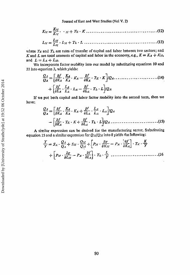
Ksr KJr Kir = --a . Jr + Tr; . K ..................................... ..(12)

Lsr = LJr . Lx + TL . L ....................................... .(13) Lsr

where TK and TL are rates of transfer of capital and labor between two sectors; and K and L are total amounts of capital and Iabor in the economy, e.g., K = KA + K v , and L = LA + Lv.

We incorporate factor mobility into our model by substituting equations 10 and 11 into equation 3, which yields:

If we put both capital and labor factor mobility into the second term, then we have :

A similar expression can be derived for the manufacturing sector. Substituting equation 15 and a similar expression for Q.u/QJr into 8 yields the following:

80

Dow

nloa

ded

by [

Uni

vers

ity o

f St

rath

clyd

e] a

t 19:

52 0

6 O

ctob

er 2

014

determinants of internal migration in korea

Documents